Random variables

Petter Mostad

2005.09.19

Repetition

• Sample space, set theory, events, probability

• Conditional probability, Bayes theorem, independence, odds

• Random variables, pdf, cdf, expected value, variance

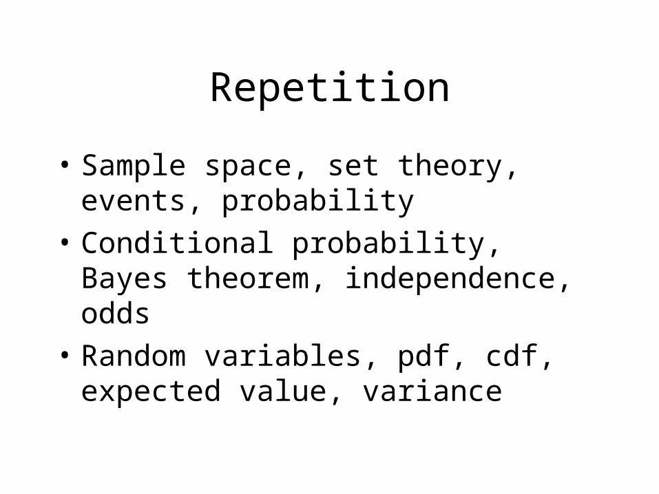
Some combinatorics

• How many ways can you make ordered selections of s objects from n objects? Answer: n*(n-1)*(n-2)*…*(n-s+1))

• How many ways can you order n objects? Answer: n*(n-1)*…*2*1 = n! (”n faculty”)

• How many ways can you make unordered selections of s objects from n objects? Answer: ( 1) ( 1) !

! !( )!

nn n n s n

ss s n s

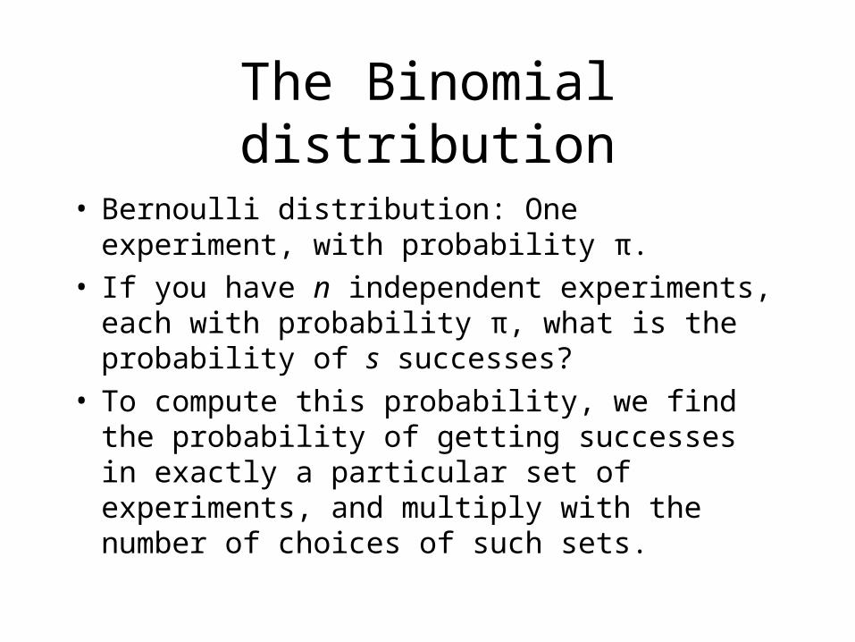
The Binomial distribution

• Bernoulli distribution: One experiment, with probability π.

• If you have n independent experiments, each with probability π, what is the probability of s successes?

• To compute this probability, we find the probability of getting successes in exactly a particular set of experiments, and multiply with the number of choices of such sets.

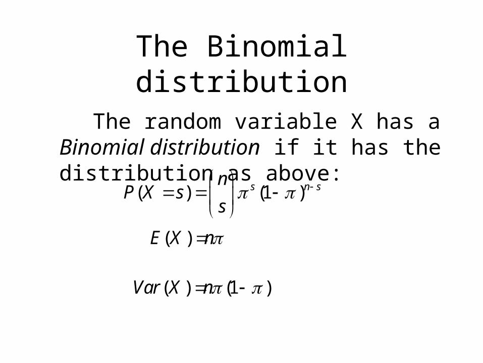
The Binomial distribution

The random variable X has a Binomial distribution if it has the distribution as above:

( ) (1 )s n snP X s

s

( )E X n

( ) (1 )Var X n

Example

• In a clinic, 20% of the patients come because of problem X. If the clinic treats 20 patients one day, what is the probability that zero, one, or two patients will come because of problem X?

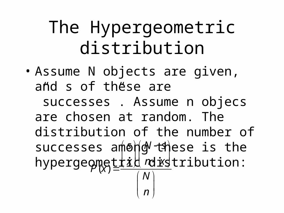
The Hypergeometric distribution

• Assume N objects are given, and s of these are ”successes”. Assume n objecs are chosen at random. The distribution of the number of successes among these is the hypergeometric distribution:

( )

s N s

x n xP x

N

n

Example

• A class consists of 20 girls and 10 boys. A group of 5 students is selected at random. What is the probability that it will contain 0, 1, or 2 girls?

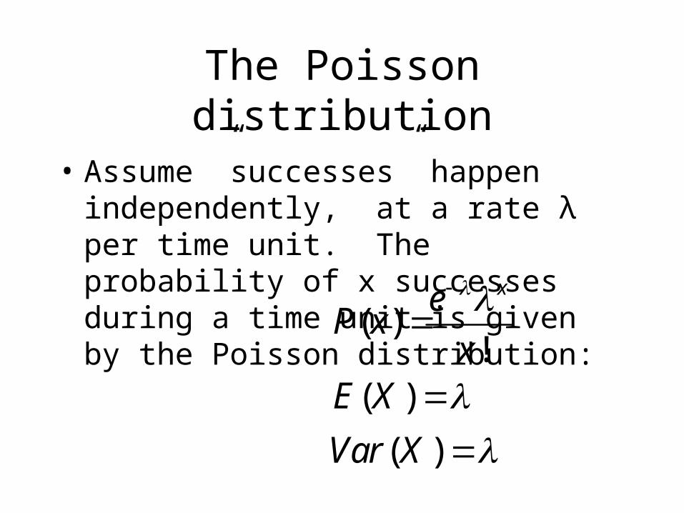
The Poisson distribution

• Assume ”successes” happen independently, at a rate λ per time unit. The probability of x successes during a time unit is given by the Poisson distribution:

( )!

( )

( )

xeP x

xE X

Var X

Example

• Assume patients come to an emergency room at an average rate of 1 per hour. What is the probability that 3 or more patients will come within a particular hour?

The Poisson and the Binomial

• It is possible to construct a Binomial variable quite similar to a Poisson variable:– Subdivide time unit into n subintervals. – Set the probability of success in each subinterval to λ/n. – Letting n goto infinity, the two processes become

identical.

• The above argument can be used to find the formula for the Poisson distribution.

• Also: Poisson approximates Binomial when n is large and p is small.

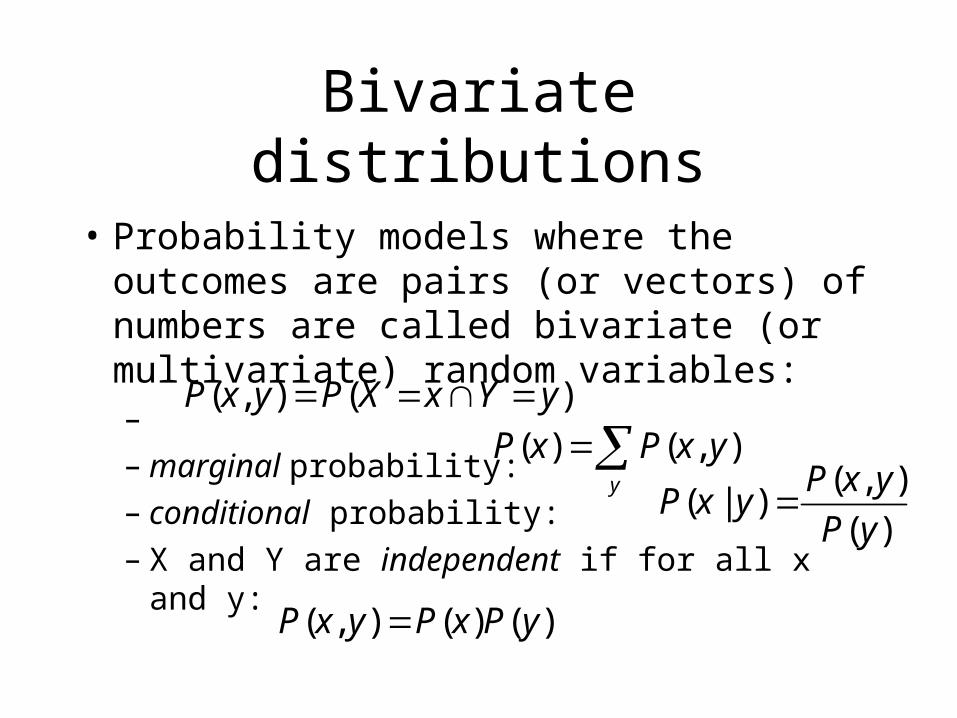
Bivariate distributions

• Probability models where the outcomes are pairs (or vectors) of numbers are called bivariate (or multivariate) random variables:– – marginal probability: – conditional probability: – X and Y are independent if for all x and y:

( , ) ( )P x y P X x Y y ( ) ( , )

y

P x P x y( , )

( | )( )

P x yP x y

P y

( , ) ( ) ( )P x y P x P y

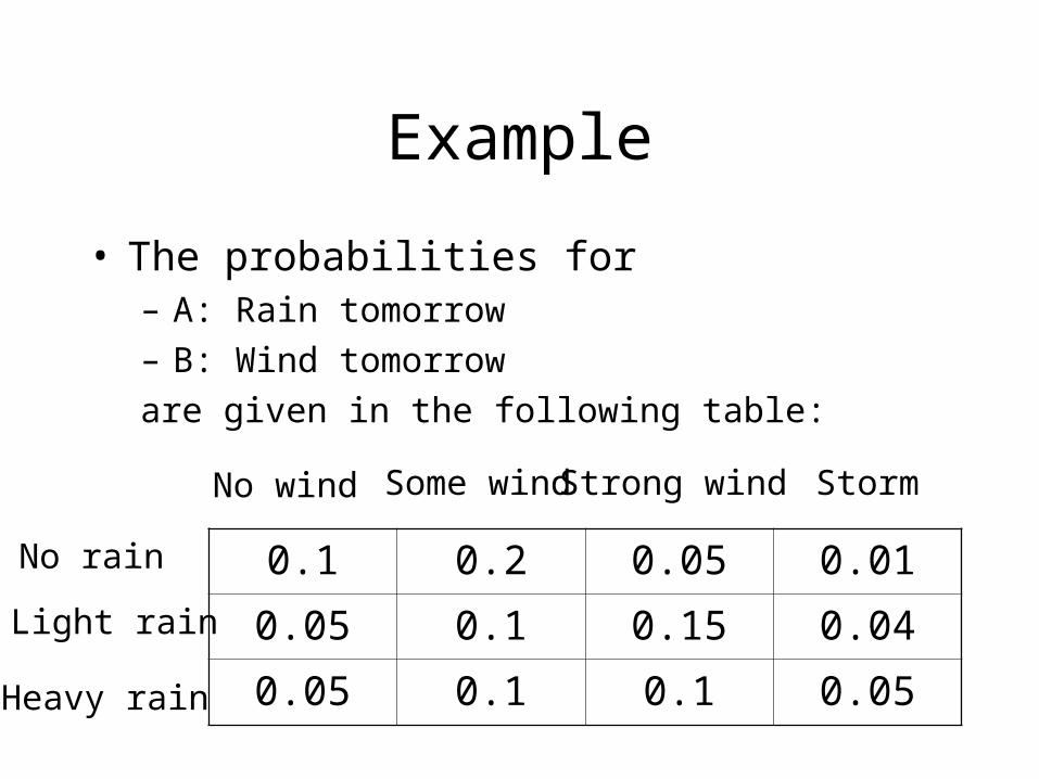
Example

• The probabilities for – A: Rain tomorrow

– B: Wind tomorrow

are given in the following table:

0.1 0.2 0.05 0.01

0.05 0.1 0.15 0.04

0.05 0.1 0.1 0.05

No rain

Light rain

Heavy rain

No wind Some wind Strong wind Storm

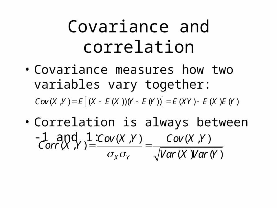
Covariance and correlation

• Covariance measures how two variables vary together:

• Correlation is always between -1 and 1:

( , ) ( ( ))( ( )) ( ) ( ) ( )Cov X Y E X E X Y E Y E XY E X E Y

( , ) ( , )( , )

( ) ( )X Y

Cov X Y Cov X YCorr X Y

Var X Var Y

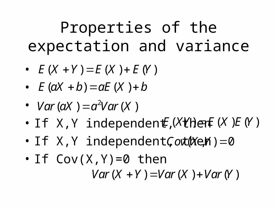
Properties of the expectation and variance

•

•

•

• If X,Y independent, then

• If X,Y independent, then

• If Cov(X,Y)=0 then

( ) ( ) ( )E X Y E X E Y ( ) ( )E aX b aE X b

2( ) ( )Var aX a Var X( ) ( ) ( )E XY E X E Y

( , ) 0Cov X Y

( ) ( ) ( )Var X Y Var X Var Y

Continuous random variables

• Used when the outcomes are best modelled as real numbers

• Probabilities are assigned to intervals of numbers; individual numbers generally have probability zero

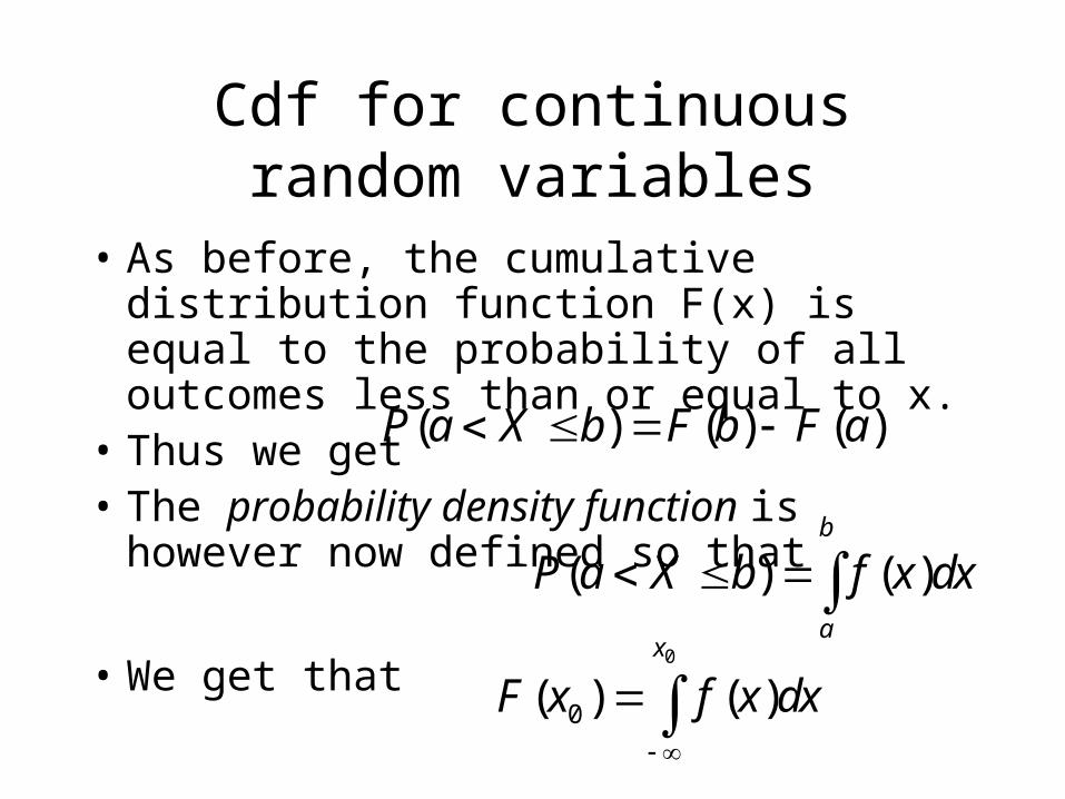
Cdf for continuous random variables

• As before, the cumulative distribution function F(x) is equal to the probability of all outcomes less than or equal to x.

• Thus we get • The probability density function is however

now defined so that

• We get that

( ) ( ) ( )P a X b F b F a

( ) ( )b

a

P a X b f x dx 0

0( ) ( )x

F x f x dx

Expectations

• The expectation of a continuous random variable X is defined as

• The variance, standard deviation, covariance, and correlation are defined exactly as before, in terms of the expectation, and thus have the same properties

( ) ( )E X xf x dx

Example: The uniform distribution on the interval [0,1]

• f(x)=1

• F(x)=x

•

•

1 1121 1

2 200 0

( ) ( )E X xf x dx xdx x

2 2

122 1 1 1

3 4 120

( ) ( ) ( )

( ) 0.5

Var X E X E X

x d x

The normal distribution

• The most used continuous probability distribution: – Many observations tend to approximately

follow this distribution– It is easy and nice to do computations with– BUT: Using it can result in wrong conclusions

when it is not appropriate

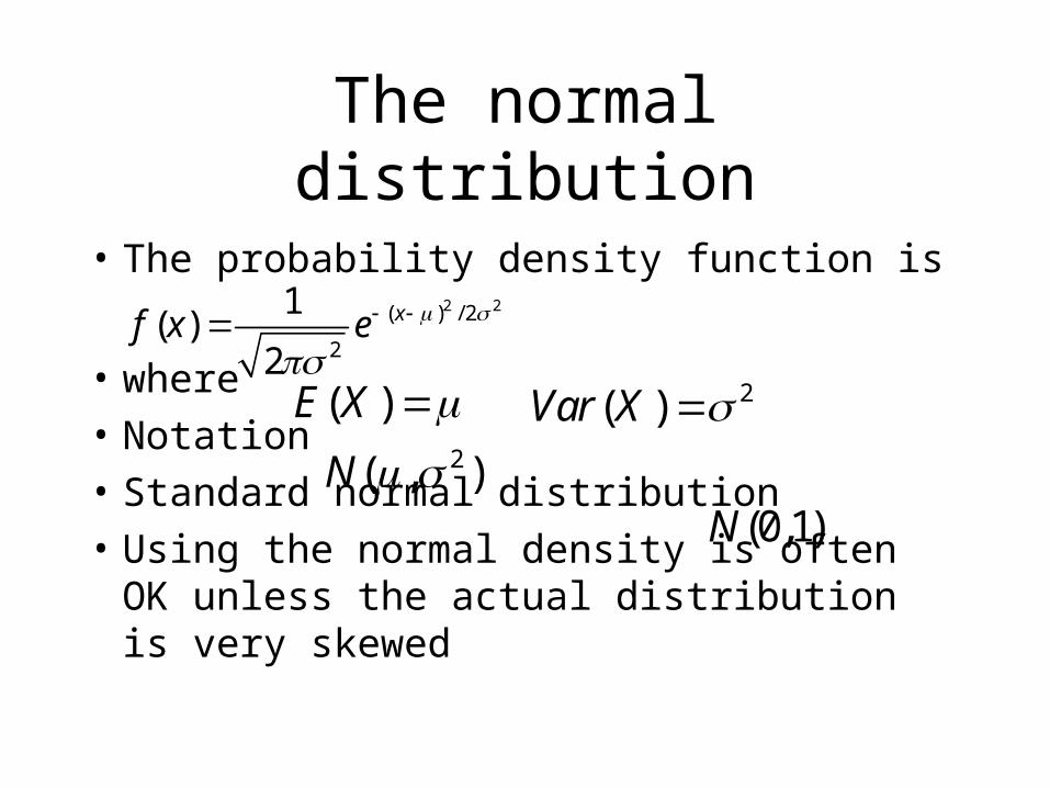
The normal distribution

• The probability density function is

• where

• Notation

• Standard normal distribution

• Using the normal density is often OK unless the actual distribution is very skewed

2 2( ) / 2

2

1( )

2

xf x e

( )E X 2( )Var X 2( , )N

(0,1)N

Normal probability plots

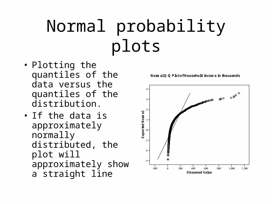
• Plotting the quantiles of the data versus the quantiles of the distribution.

• If the data is approximately normally distributed, the plot will approximately show a straight line -200 0 200 400 600 800 1 000 1 200

Observed Value

-3

-2

-1

0

1

2

3

4

Exp

ecte

d N

orm

al

Normal Q-Q Plot of Household income in thousands

The Normal versus the Binomial distribution

• When n is large and π is not too close to 0 or 1, then the Binomial distribution becomes very similar to the Normal distribution with the same expectation and variance.

• This is a phenomenon that happens for all distributions that can be seen as a sum of independent observations.

• It can be used to make approximative computations for the Binomial distribution.

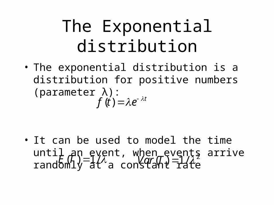
The Exponential distribution

• The exponential distribution is a distribution for positive numbers (parameter λ):

• It can be used to model the time until an event, when events arrive randomly at a constant rate

( ) tf t e

( ) 1/E T 2( ) 1/Var T