Embed Size (px)
Citation preview
Random Variables and Stochastic Processes – 0903720
Lecture#13
Dr. Ghazi Al SukkarEmail: [email protected]
Office Hours: Refer to the websiteCourse Website:
http://www2.ju.edu.jo/sites/academic/ghazi.alsukkar
1

2
Chapter 6Two Functions of Two Random Variables
Definition Joint Density and the Jacobian Examples for Continuous R.Vs Auxiliary Variables Example for Discrete R.Vs

3
Definition
• Given two random variables and with joint PDF . Given two functions and , we form new random variables and as:
• Given the joint PDF how does one obtain the joint PDF ?
• Obviously with in hand, one can find the marginal PDFs, and .
4
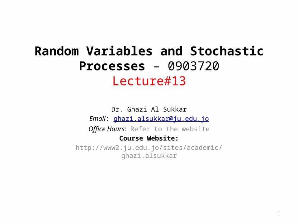
• For given and ,
• where is the region in the plane such that the inequalities and are simultaneously satisfied.
wzDyx XYwz
ZW
dxdyyxfDYXP
wYXhzYXgPwWzZPwzF
,),( , ,),(),(
),(,),()(,)(),(
x
y
wzD ,
wzD ,
5
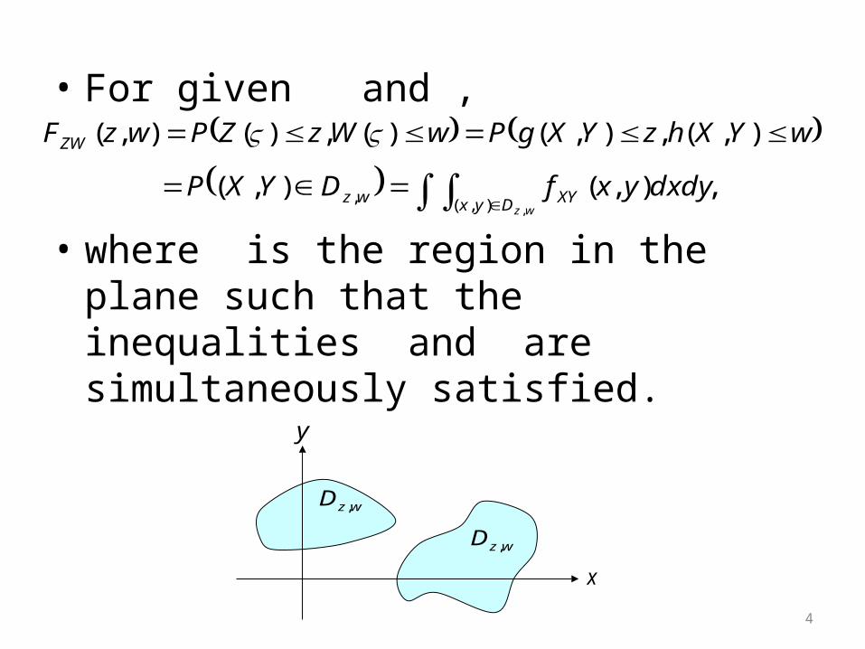
• Example: Suppose and are independent uniformly distributed random variables in the interval . Define , . Determine .
Sol.: Both and vary in the interval . Thus: We must consider two cases: and since they give rise to different regions for . (Refer to Example 6 lect.12)
X
Y
wy
),( ww
),( zz
zwa )(
X
Y
),( ww
),( zz
zwb )(
6
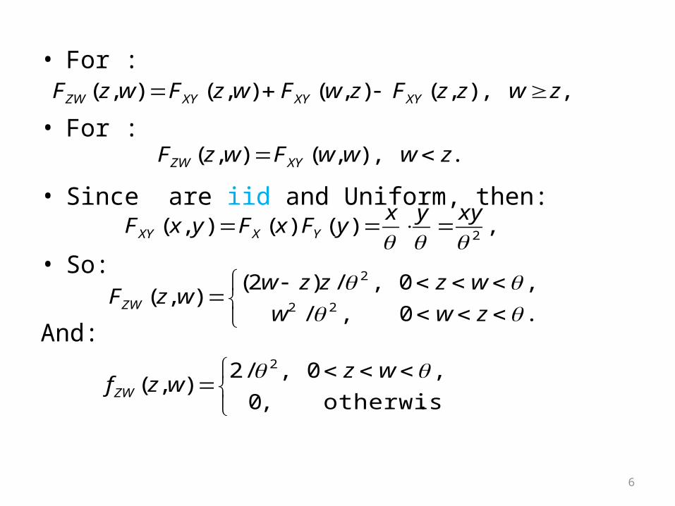
• For :
• For :
• Since are iid and Uniform, then:
• So:
And:
, , ),(),(),(),( zwzzFzwFwzFwzF XYXYXYZW
. , ),(),( zwwwFwzF XYZW
,)( )(),(2
xyyxyFxFyxF YXXY
2
2 2
(2 ) / , 0 ,( , )
/ , 0 .ZW
w z z z wF z w
w w z
.otherwise,0
,0,/2),(
2 wzwzfZW
7
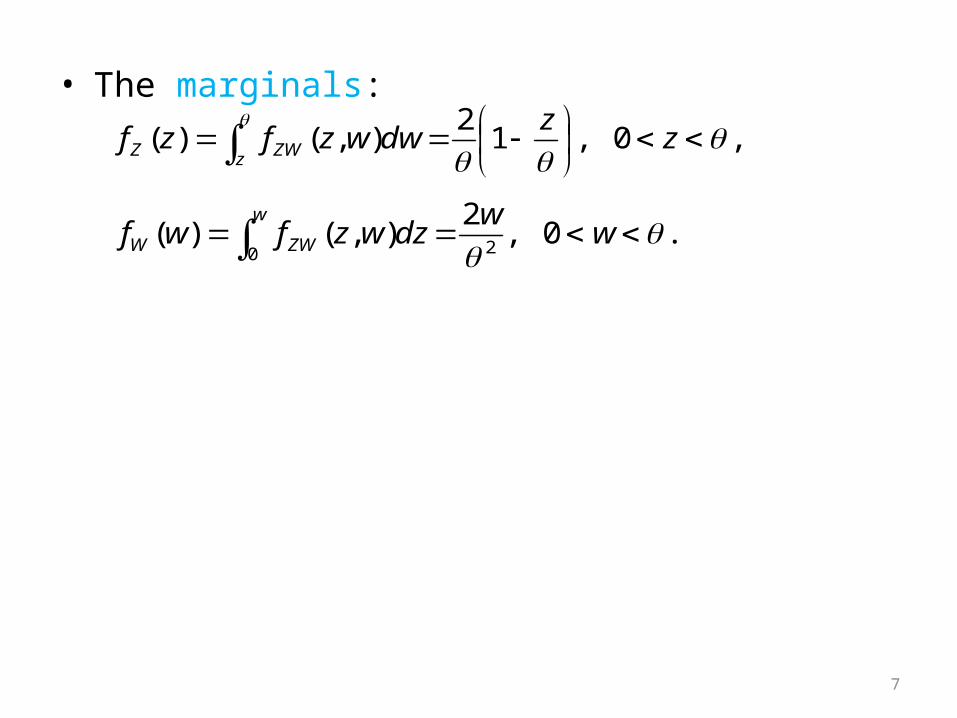
• The marginals:
,0 ,12
),()(
z
zdwwzfzf
z ZWZ
.0 ,2
),()(
0 2
w
wdzwzfwf
w
ZWW

8
Joint Density• If and are continuous and differentiable functions, then it is
possible to develop a formula to obtain the joint PDF directly. • Consider the equations:
, For a given point we can have many solutions. Let us say
represent these multiple solutions such that
• Consider the problem of evaluating the probability
),,( , ),,( ),,( 2211 nn yxyxyx
.),( ,),( wyxhzyxg iiii
. ),(,),(
,
wwYXhwzzYXgzP
wwWwzzZzP

9
• We can rewrite this as:
• To translate this probability in terms of we need to evaluate the equivalent region for in the plane.
.),(, wzwzfwwWwzzZzP ZW
z
(a)
w
),( wz
z
www
zz
(b)
x
y1
2
i
n
),( 11 yx
),( 22 yx
),( ii yx
),( nn yx
10
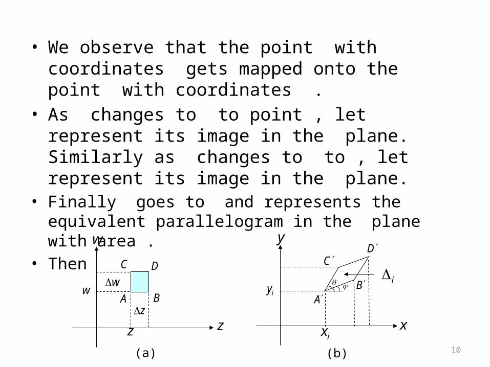
• We observe that the point with coordinates gets mapped onto the point with coordinates .
• As changes to to point , let represent its image in the plane. Similarly as changes to to , let represent its image in the plane.
• Finally goes to and represents the equivalent parallelogram in the plane with area .
• Then
(a)
w
Az
ww
B
zz
C D
(b)
y
Aiy B
xix
CD
i

11
• Then• To simplify, we need to evaluate the area of the
parallelograms in terms of .• Towards this, let and denote the inverse transformation,
so that:
• As the point goes to the point , the point , the point and the point . Hence the respective and coordinates of are given by:
• and
.),(),(
i
iiiXYZW wzyxfwzf
).,( ),,( 11 wzhywzgx ii
,),(),( 1111 z
z
gxz
z
gwzgwzzg i
.),(),( 1111 z
z
hyz
z
hwzhwzzh i
12
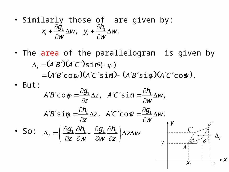
• Similarly those of are given by:
• The area of the parallelogram is given by
• But:
• So:
. , 11 ww
hyw
w
gx ii
. cos sinsin cos
)sin(
CABACABA
CABAi
.cos ,sin
,sin ,cos
11
11
ww
gCAz
z
hBA
ww
hCAz
z
gBA
wzz
h
w
g
w
h
z
gi
1111
y
Aiy B
xix
CD
i

13
• And
• The right side represents the Jacobian of the transformation• Thus
• By substitution, we get
• since
w
h
z
h
w
g
z
g
z
h
w
g
w
h
z
g
wzi
11
11
1111 det
).,( ),,( 11 wzhywzgx ii 1 1
1 1
( , ) det .
g g
z wJ z w
h h
z w
,),(|),(|
1),(|),(|),(
iiiXY
iiiiiXYZW yxf
yxJyxfwzJwzf
|),(|
1 |),(|
ii yxJwzJ
14
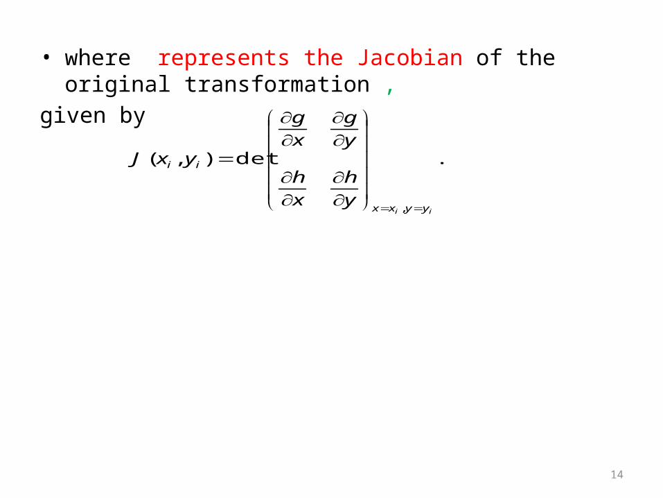
• where represents the Jacobian of the original transformation ,
given by
.det),(
, ii yyxx
ii
y
h
x
h
y
g
x
g
yxJ

15
• Example: Suppose and are zero mean independent Gaussian R.Vs with common variance . Define , , where Obtain .
Sol.:
Since if is a solution pair so is
Substituting this into z, we get
And
.2
1),(
222 2/)(2
yx
XY eyxf
,2/||),/(tan),(;),( 122 wxyyxhwyxyxgz
).tan(or ),tan( wxywx
y
).cos( or ),sec( tan1 222 wzxwxwxyxz
).sin()tan( wzwxy
16
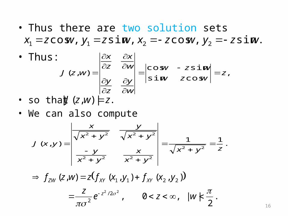
• Thus there are two solution sets
• Thus:
• so that • We can also compute
.sin ,cos ,sin ,cos 2211 wzywzxwzywzx
,cossin
sincos),( z
wzw
wzw
w
y
z
y
w
x
z
x
wzJ
.|),(| zwzJ
.11
),(22
2222
2222
zyx
yx
x
yx
y
yx
y
yx
x
yxJ
.2
|| ,0 ,
),(),(),(
22 2/2
2211
wzez
yxfyxfzwzf
z
XYXYZW

17
• Thus
Which represents a Rayleigh R.V. with parameter and
• which represents a uniform R.V. in the interval . Moreover by direct computation
implying that Z and W are independent.• We summarize these results in the following statement: If X
and Y are zero mean independent Gaussian random variables with common variance, then has a Rayleigh distribution and has a uniform distribution. Moreover these two derived r.vs are statistically independent.
,0 ,),()(22 2/
2
2/
2/
zez
dwwzfzf zZWZ
,2
|| ,1
),()(
0
wdzwzfwf ZWW
)()(),( wfzfwzf WZZW
18
• Alternatively, with X and Y as independent zero mean R.V.s, represents a complex Gaussian R.V. But
• where and , except that to hold good on the entire complex plane we must have and hence it follows that the magnitude and phase of a complex Gaussian r.v are independent with Rayleigh and uniform distributions respectively.
,jWZejYX
19
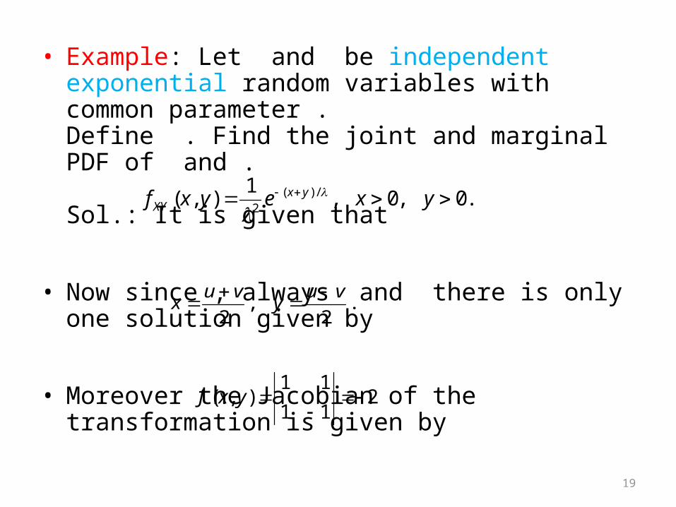
• Example: Let and be independent exponential random variables with common parameter . Define . Find the joint and marginal PDF of and . Sol.: It is given that
• Now since , always and there is only one solution given by
• Moreover the Jacobian of the transformation is given by
.0 ,0 ,1
),( /)(2
yxeyxf yxXY
.2
,2
vuy
vux
2 11
1 1 ),(
yxJ

20
• And hence
• This gives
And
• Notice that in this case the R.V.s U and V are not independent.
, || 0 ,2
1),( /
2 uvevuf u
UV
,0 ,2
1),()( /
2
/2
ueu
dvedvvufuf uu
u
uu
u UVU
/ | |/
2 | | | |
1 1( ) ( , ) , .
2 2u v
V UVv vf v f u v du e du e v
21
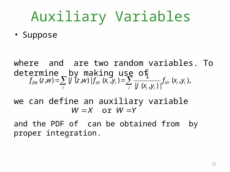
Auxiliary Variables • Suppose
where and are two random variables. To determine by making use of
we can define an auxiliary variable
and the PDF of can be obtained from by proper integration.
,),(|),(|
1),(|),(|),(
iiiXY
iiiiiXYZW yxf
yxJyxfwzJwzf
YWXW or
22
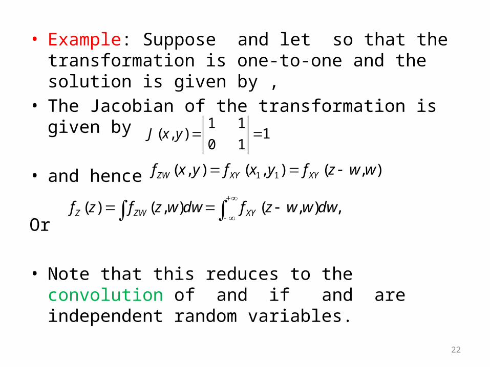
• Example: Suppose and let so that the transformation is one-to-one and the solution is given by ,
• The Jacobian of the transformation is given by
• and hence
Or
• Note that this reduces to the convolution of and if and are independent random variables.
1 1 0
1 1 ),( yxJ
),(),(),( 11 wwzfyxfyxf XYXYZW
,),(),()( dwwwzfdwwzfzf XYZWZ
23
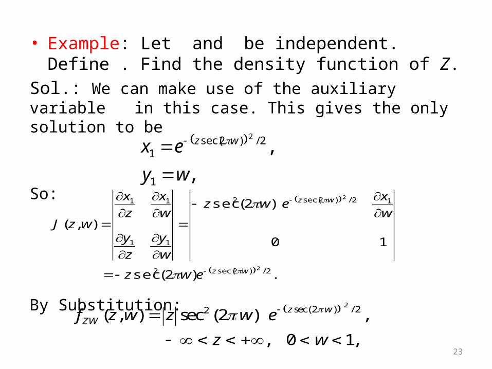
• Example: Let and be independent. Define . Find the density function of Z.
Sol.: We can make use of the auxiliary variable in this case. This gives the only solution to be
So:
By Substitution:
,
,
1
2/)2sec(1
2
wy
ex wz
.)2(sec
10
)2(sec
),(
2/)2sec(2
12/)2sec(2
11
11
2
2
wz
wz
ewz
w
xewz
w
y
z
y
w
x
z
x
wzJ
2sec(2 ) / 22( , ) sec (2 ) ,
, 0 1,
z wZWf z w z w e
z w
24
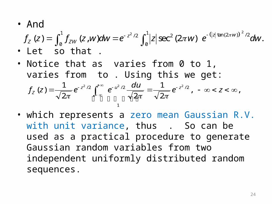
• And
• Let so that . • Notice that as varies from 0 to 1, varies from to . Using this
we get:
• which represents a zero mean Gaussian R.V. with unit variance, thus . So can be used as a practical procedure to generate Gaussian random variables from two independent uniformly distributed random sequences.
22 1 1 tan(2 ) / 2/ 2 2
0 0( ) ( , ) sec (2 ) .z wz
Z ZWf z f z w dw e z w e dw
, ,2
1
2
2
1)( 2/
1
2/2/ 222
zedu
eezf zuzZ
25
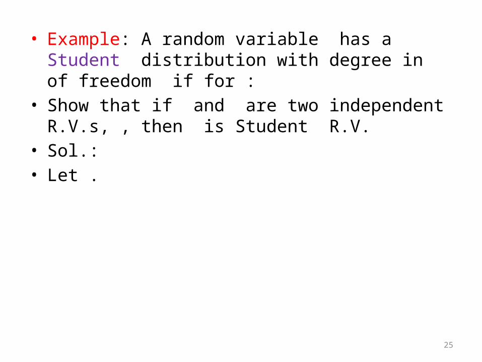
• Example: A random variable has a Student distribution with degree in of freedom if for :
• Show that if and are two independent R.V.s, , then is Student R.V.
• Sol.: • Let .

26
Put and integrating we get: • For it becomes Cauchy R.V.
27
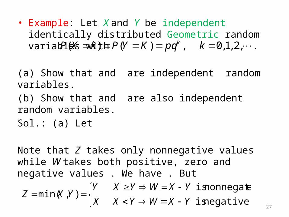
• Example: Let X and Y be independent identically distributed Geometric random variables with
(a) Show that and are independent random variables.(b) Show that and are also independent random variables. Sol.: (a) Let Note that Z takes only nonnegative values while W takes both positive, zero and negative values . We have . But
.,2 ,1 ,0 ,)()( kpqKYPkXP k
negative. is
enonnegativ is ),min(
YXWYXX
YXWYXYYXZ
28
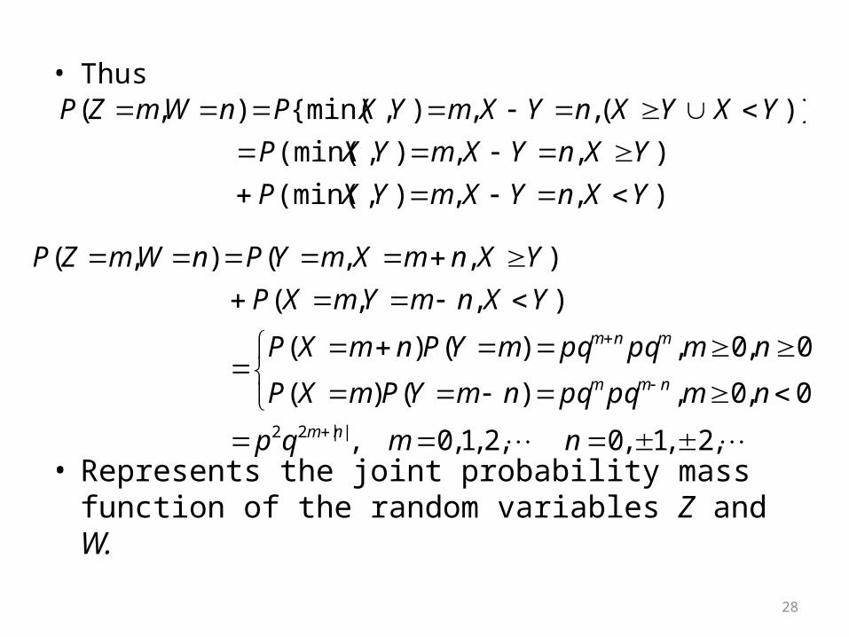
• Thus
• Represents the joint probability mass function of the random variables Z and W.
),,),(min(
),,),(min(
)} (,,),{min(),(
YXnYXmYXP
YXnYXmYXP
YXYXnYXmYXPnWmZP
,2 ,1 ,0 ,2 ,1 ,0 ,
0,0,)()(
0,0,)()(
),,(
),,( ),(
||22
nmqp
nmpqpqnmYPmXP
nmpqpqmYPnmXP
YXnmYmXP
YXnmXmYPnWmZP
nm
nmm
mnm
29
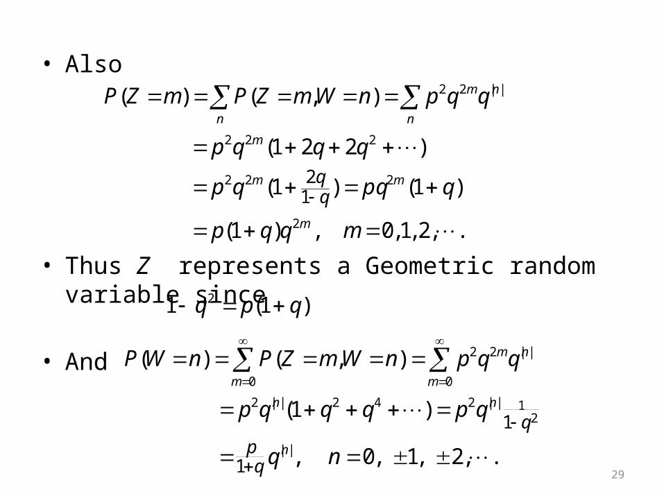
• Also
• Thus Z represents a Geometric random variable since
• And
.,2 ,1 ,0 ,)1(
)1()1(
)221(
),()(
2
222
222
||22
12
mqqp
qpqqp
qqqp
qqpnWmZPmZP
m
mm
m
n n
nm
),1(1 2 qpq
2 2 | |
0 0
2 | | 2 4 2 | | 12
| |
1
1
( ) ( , )
(1 )
, 0, 1, 2, .
m n
m m
n n
n
qpq
P W n P Z m W n p q q
p q q q p q
q n
30
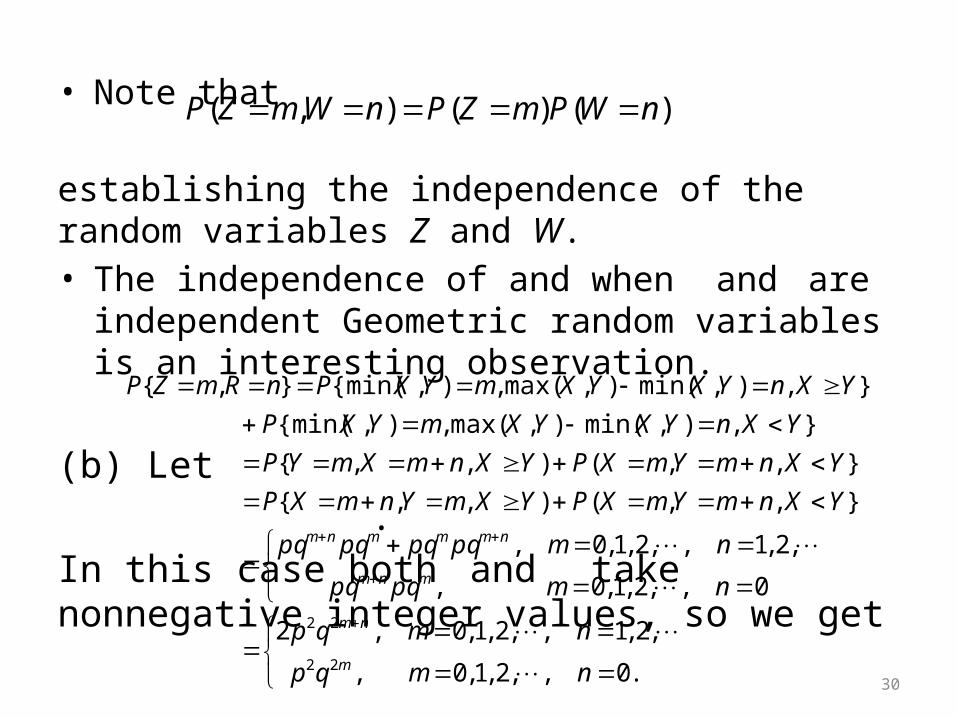
• Note that
establishing the independence of the random variables Z and W.• The independence of and when and are independent
Geometric random variables is an interesting observation.
(b) Let . In this case both and take nonnegative integer values, so we get
),()(),( nWPmZPnWmZP
.0 ,,2 ,1 ,0 ,
,2 ,1 ,,2 ,1 ,0 ,2
0 ,,2 ,1 ,0 ,
,2 ,1 ,,2 ,1 ,0 ,
} ,,() ,,{
} ,,() ,,{
} ,),min(),max( ,),{min(
} ,),min(),max( ,),{min(},{
22
22
nmqp
nmqp
nmpqpq
nmpqpqpqpq
YXnmYmXPYXmYnmXP
YXnmYmXPYXnmXmYP
YXnYXYXmYXP
YXnYXYXmYXPnRmZP
m
nm
mnm
nmmmnm
31
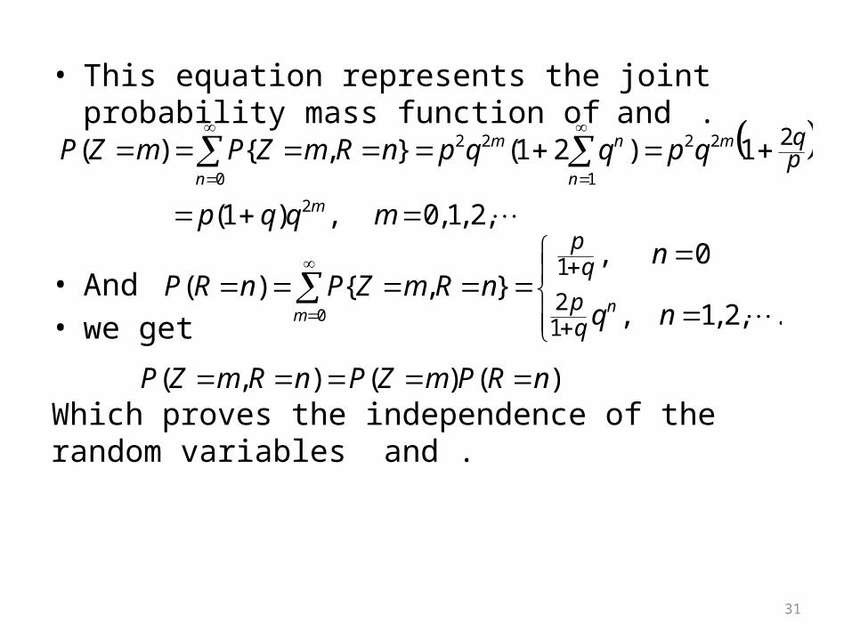
• This equation represents the joint probability mass function of and .
• And • we get
Which proves the independence of the random variables and .
,2 ,1 ,0 ,)1(
1)21(},{)(
2
0
22
1
22 2
mqqp
qpqqpnRmZPmZP
m
n
m
n
nmpq
.,2 ,1 ,
0 , },{)(
12
1
0 nq
nnRmZPnRP
nm
qp
qp
)()(),( nRPmZPnRmZP