Embed Size (px)
Citation preview
Project Number: CS-GXS-0801
Random Search Algorithms
a Major Qualifying Project Report submitted to the Faculty of the
WORCESTER POLYTECHNIC INSTITUTE
in partial fulfillment of the requirements for the
Degree of Bachelor of Science by
__________________________________________________ James H. Brodeur
__________________________________________________ Benjamin E. Childs
April 21, 2008
___________________________________________________________ Professor Gábor N. Sárközy, Major Advisor
___________________________________________________________ Professor Stanley M. Selkow, Co-Advisor
i
Abstract
In this project we designed and developed improvements for the random search
algorithm UCT with a focus on improving performance with directed acyclic graphs and
groupings. We then performed experiments in order to quantify performance gains with
both artificial game trees and computer Go. Finally, we analyzed the outcome of the
experiments and presented our findings. Overall, this project represents original work in
the area of random search algorithms on directed acyclic graphs and provides several
opportunities for further research.
[1] [2] [3] [4] [5] [6] [7] [8] [9] [10] [11] [12] [13] [14] [15] [16] [17]

ii
Acknowledgments
We would like to express our gratitude to those individuals whose assistance,
hospitality, and advice made the completion of this project successful and enjoyable:
Professor Gábor N. Sárközy, main advisor
Professor Stanley M. Selkow, co-advisor
MTA SZTAKI
o MLHCI Group
Levente Kocsis, SZTAKI liaison
András György, SZTAKI liaison
Petronella Hajdú, SZTAKI colleague
o Internet Applications Department
o Adam Kornafeld, SZTAKI colleague
Worcester Polytechnic Institute
Lukasz Lew, LibEGO Maintainer
iii
Table of Contents
Abstract ......................................................................................................................................... i
Acknowledgments ................................................................................................................... ii
Table of Figures ......................................................................................................................... v
Table of Tables ......................................................................................................................... vi
Table of Equations .................................................................................................................. vi
Chapter 1: Background ....................................................................................................... 1
1.1 Search Algorithms ..................................................................................................................................................... 2
1.2 The Rules of Go ........................................................................................................................................................... 8
1.3 Algorithms for Go ...................................................................................................................................................... 9
1.4 Investigations into UCT Enhancements......................................................................................................... 15
1.4.1 UCB Modifications ............................................................................................................................................ 15
1.4.2 MOGO ..................................................................................................................................................................... 16
1.4.3 Directed Acyclic Graphs................................................................................................................................. 17
1.4.4 Grouping ............................................................................................................................................................... 18
1.5 Conclusion .................................................................................................................................................................. 19
Chapter 2: Development ................................................................................................... 20
2.1 Details of Existing Codebases ............................................................................................................................. 20
2.1.1 PGame .................................................................................................................................................................... 20
2.1.2 LibEGO ................................................................................................................................................................... 22
2.2 UCT on Directed Acyclic Graphs ....................................................................................................................... 23
2.2.1 Behavior of UCT-DAG ..................................................................................................................................... 25
2.2.2 Transposition Table ........................................................................................................................................ 28
2.3 UCT-DAG Implementation ................................................................................................................................... 28
2.3.1 PGame .................................................................................................................................................................... 29
2.3.2 LibEGO ................................................................................................................................................................... 31
2.4 Grouping ...................................................................................................................................................................... 34
2.5 Grouping Implementation ................................................................................................................................... 35
2.5.1 PGame .................................................................................................................................................................... 36
2.5.2 LibEGO ................................................................................................................................................................... 37
2.6 Conclusion .................................................................................................................................................................. 40
Chapter 3: Experiments .................................................................................................... 42
3.1 Artificial Game Trees ............................................................................................................................................. 43
3.1.1 UCT on Directed Acyclic Graphs ................................................................................................................ 45
3.1.2 UCT-DAG on Grouped Trees ........................................................................................................................ 48
3.1.3 Conclusion ........................................................................................................................................................... 56
iv
3.2 Computerized Go ..................................................................................................................................................... 57
3.2.1 Go on a 9x9 Board ............................................................................................................................................ 58
3.2.2 Go on a 13x13 Board ....................................................................................................................................... 59
3.2.3 Conclusion ........................................................................................................................................................... 62
Chapter 4: Conclusion ........................................................................................................ 63
4.1 Findings ....................................................................................................................................................................... 63
4.1.1 UCT-DAG can improve performance of UCT on complex DAGs and performs equally to UCT on simple DAGs........................................................................................................................................ 63
4.1.2 Highly correlated, complete groupings dramatically improve performance of UCT on trees with high branching factors. ............................................................................................................ 64
4.1.3 Highly accurate, complete groupings with group overlap dramatically improve performance of UCT on any tree. ............................................................................................................... 65
4.1.4 Multiple less-accurate groups, with group overlap, perform similarly to a single more-accurate group. .................................................................................................................................................. 65
4.1.5 Accurate groupings in conjunction with UCT-DAG improve the performance of LibEGO vs GnuGo on larger boards. .......................................................................................................................... 66
4.1.6 The size of the UCT-DAG transposition table may be sensitive to branching factor. ......... 67
4.2 Future Research ....................................................................................................................................................... 67
4.2.1 UCT-DAG with Multi-Path Update ............................................................................................................ 68
4.2.2 Transposition Table ........................................................................................................................................ 68
4.2.3 Online or Offline Determination of Group Biases & Parameter Tuning ................................... 69
4.2.4 Using the GRID as a mechanism for Machine Learning with UCT / Grouping ...................... 71
4.2.5 UCT/Monte-Carlo Simulation Split: LibEGO & PGame .................................................................... 72
4.3 Summary ..................................................................................................................................................................... 72
References ................................................................................................................................ 76
Appendix A Artificial Game Tree Experiment Plan ................................................. 78
Appendix B Computer Go Experiment Plan ............................................................... 79
Appendix C Artificial Game Trees Experiment Results ......................................... 80
Appendix D Computer Go Experiment Results ......................................................... 84
Appendix E Developer Comments ................................................................................. 86
v
Table of Figures
Figure 1.1 - UCT Algorithm ....................................................................................................................................................................... 12
Figure 1.2 - UCT Experiment on Artificial Game Tree .................................................................................................................. 14
Figure 1.3 - Example Directed Acyclic Graph.................................................................................................................................... 18
Figure 2.1 - UCT on a Game Tree ............................................................................................................................................................ 23
Figure 2.2 - UCT treating Game as a DAG ........................................................................................................................................... 24
Figure 2.3 - UCT-DAG on DAG .................................................................................................................................................................. 24
Figure 2.4 - UCT with Transposition Table ........................................................................................................................................ 32
Figure 2.6 – UCT with Transposition Table and Grouping ......................................................................................................... 38
Figure 3.1 - Average Error vs. UCT-DAG with varying DAG Combination on 2x20 Tree .............................................. 46
Figure 3.2 - Average Error vs. UCT (Base) with varying DAG Combination on 2x20 Tree ........................................... 46
Figure 3.3 – Base Average Error / Average Error for UCT with Varying DAG Combination on 2x20 Tree .......... 47
Figure 3.4 - Base Average Error / Average Error for UCT with Varying DAG Combination on 10x6 Tree ........... 48
Figure 3.5– Average Error vs. Group Bias on 10x6 Tree ............................................................................................................. 50
Figure 3.6 – Base Average Error / Average Error vs. Group Bias on 10x6 Tree ............................................................... 51
Figure 3.7– Average Error vs. Group Bias on 10x6 Tree with Group Overlap ................................................................... 52
Figure 3.8– Base Average Error / Average Error vs. Group Bias on 2x20 Tree ................................................................ 53
Figure 3.9– Base Average Error / Average Error vs. Group Bias on 2x20 Tree with Group Overlap ...................... 54
Figure 3.10 - Base Average Error / Average Error vs. Number of Groups and Group Accuracy with Group Size 100% ................................................................................................................................................................................................................... 55
Figure 3.11 - Base Average Error / Average Error vs. Number of Groups and Group Accuracy, with Group Size 25% ..................................................................................................................................................................................................................... 56
Figure 3.12 - Results of Go Experiment on 9x9 board with 20 second moves .................................................................. 58
Figure 3.13- Results of Go Experiment on 13x13 board with 40 second moves .............................................................. 60
Figure 3.14 – Results of Go Experiment on 13x13 board with 40 second moves (90% confidence intervals) . 61
Figure C.1 - Base Average Error / Average Error for UCT with Varying DAG Combination on 4x10 Tree ........... 80
Figure C.2 - Base Average Error / Average Error for UCT with Varying DAG Combination on 4x10 Tree ........... 80
Figure C.3 – Average Error vs. Group Bias on 6x8 Tree ............................................................................................................... 81
Figure C.4 - Base Average Error / Average Error vs. Group Bias on 6x8 Tree................................................................... 81
Figure C.5 - Average Error vs. Group Bias on 10x6 Tree with Group Overlap ................................................................... 82
Figure C.6 - Base Average Error / Average Error vs. Group Bias on 6x8 Tree................................................................... 82
Figure C.7 - Base Average Error / Average Error vs. Group Bias on 10x6 Tree ................................................................ 83
Figure C.8 - Base Average Error / Average Error vs. Number of Groups and Group Accuracy with Group Size 50% ..................................................................................................................................................................................................................... 83
Figure D.1 - Results of Go Experiment on 9x9 board with 10 second moves.................................................................... 84
Figure D.2 - Results of Go Experiment on 13x13 board with 80 second moves ............................................................... 84
Figure D.3 - Results of Go Experiment on 13x13 board with 160 second moves ............................................................ 85
vi
Table of Tables
Table 2.1 – Implemented Groupings ..................................................................................................................................................... 40
Table 3.1 - LibEGO Configurations for Computer Go Experiments ......................................................................................... 57
Table A.1 - Artificial Game Tree Experimental Parameters ....................................................................................................... 78
Table B.1 GnuGo Experiment Parameters .......................................................................................................................................... 79
Table of Equations
Equation 1.1 – UCB1 Node Selection Formula [2] ............................................................................................................................ 7
Equation 3.1 – Standard Deviation of Normal Approximation to Binomial Distribution ............................................. 42
1
Chapter 1: Background
In the past, Chess has served as one of the most popular games for which automated
opponents have been created, climaxing in the defeat of the famed Russian chess
grandmaster Garry Kasparov in 1997 by the purpose-built system Deep Blue. Since then,
interests in human versus computer chess competitions have waned. The last high-profile
human vs. computer match ended in grandmaster Vladimir Kramnik’s 2006 loss to a
system comparable to a modern tower PC, despite the fact that he had received a copy to
practice against [12]. Speaking in relation to computerized chess’ success, McGill University
computer science professor Monty Newborn (who arranged the Kasparov vs. Deep Blue
matchup) said, “I don’t know what one could get out of it at this point. The science is done”
[12]. The East Asian board game Go, on the other hand, is coming to be of interest now that
chess is “solved” and a new computational challenge is desired.
Chess-playing algorithms generally rely on an alpha-beta search to offer
improvements over traditional min-max searches, which typically struggle with play trees
that have a high branching factor. To quickly compare the challenge of solving chess versus
Go, consider the boards. In Chess, there are, on average, about 35 moves to inspect for any
given position. With a typical game of Go on a 9x9 board (the smallest typical play format)
there are 40. The “large” size boards used by human professionals are 19x19, with an
average branching factor of about 200.
With such a high branching factor compared to chess and the nature of play, Go is a
significantly harder game to “solve” algorithmically, to the point that up until recently
computers struggled to defeat human players even on a small 9x9 board (even if they have
2
had as little as one year of practice). There are simply too many possible options, at every
stage of the game; the branching factor is far too high, compared to chess or other
applications, to manage easily. More recently the use of a random search algorithm, named
UCT, has proven successful in improving the performance of computers as applied to Go.
Originally proposed by Levente Kocsis and Csaba Szepesvari [11], its use in Go was
publicized in the Economist [1] and Reuters [9]. Thus, in recent years, experimentation
with playing Go has gained interest, especially given that the study of computerized chess
is now essentially complete. In this project we developed and tested two new modifications
to the base UCT algorithm to increase its accuracy, both discussed later in detail, resulting
in the algorithm known as UCT-DAG.
1.1 Search Algorithms
In artificial intelligence or decision-making adversarial searching (a search where
there is another person trying to “win” the selections), representing the possible positions
with a tree is a common method. This generally works well when there are fixed rules and
small state descriptions, such as what is encountered with a board game (such as chess or
Go). Nodes of the tree typically represent the board positions. The game tree is the set of
possible future board positions, where each node is a description of the board
configuration. Each link in the tree represents a move by one of the players down to the
next level and each alternating level represents the other player’s possible situations. An
exhaustive search is often impossible, even on powerful machines.
Chess, the classic example, has 10120 possible branches in its game tree [17 p. 118],
which would be impractical to search through completely (and as stated earlier, this pales
3
in comparison to Go). Instead, a look-ahead procedure that will evaluate upcoming moves
is needed. This requires the identification of all possible legal moves, perhaps some filter to
sort out patently wrong moves that can be immediately identified, a function to evaluate
the outcome, and a way to prune bad moves. Legal moves may be selected using some kind
of random procedure, or biased in terms of some metric/rule or predefined knowledge (for
example, a rule such as “always move a pawn first”).
One evaluation procedure, known as minimax, focuses on a manner of position
evaluation where one player has a better position through some kind of a heuristic. The
goal is minimizing the opponent’s score while maintaining as high a score as possible. The
metrics involved can be weighted to consider the differences between move freedom and
piece count, for example. This method assumes players will select the best option available.
It functions by checking the bottom of the tree and performing evaluation, then going back
up to select paths that will prevent or avoid the best moves for the opponent. Because tree
searches alternate layers of players’ moves, the minimax search alternates between
minimizing levels (minimizing opponent scoring) and maximizing layers of the tree
(maximizing the player’s own scoring).
By reverse-engineering the moves that led to the enemy’s worst follow-up in this
manner—and allowed for the player’s best advantage—a successful path is deduced and
the appropriate move for the level is made. Large trees make this process computationally
expensive, so the storage of calculated data is often used, and pre-generated tables for
opening and end-game moves may be implemented (this is especially the case in chess).
Data calculated mid-game is often stored in a “transposition table,” which maps a hash of
board data to the parameters which are of interest for the search (such as player scoring).
4
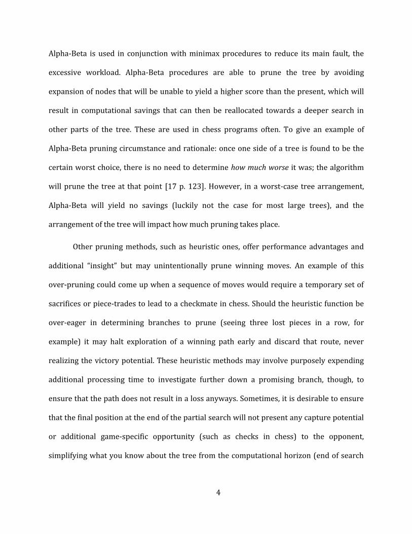
Alpha-Beta is used in conjunction with minimax procedures to reduce its main fault, the
excessive workload. Alpha-Beta procedures are able to prune the tree by avoiding
expansion of nodes that will be unable to yield a higher score than the present, which will
result in computational savings that can then be reallocated towards a deeper search in
other parts of the tree. These are used in chess programs often. To give an example of
Alpha-Beta pruning circumstance and rationale: once one side of a tree is found to be the
certain worst choice, there is no need to determine how much worse it was; the algorithm
will prune the tree at that point [17 p. 123]. However, in a worst-case tree arrangement,
Alpha-Beta will yield no savings (luckily not the case for most large trees), and the
arrangement of the tree will impact how much pruning takes place.
Other pruning methods, such as heuristic ones, offer performance advantages and
additional “insight” but may unintentionally prune winning moves. An example of this
over-pruning could come up when a sequence of moves would require a temporary set of
sacrifices or piece-trades to lead to a checkmate in chess. Should the heuristic function be
over-eager in determining branches to prune (seeing three lost pieces in a row, for
example) it may halt exploration of a winning path early and discard that route, never
realizing the victory potential. These heuristic methods may involve purposely expending
additional processing time to investigate further down a promising branch, though, to
ensure that the path does not result in a loss anyways. Sometimes, it is desirable to ensure
that the final position at the end of the partial search will not present any capture potential
or additional game-specific opportunity (such as checks in chess) to the opponent,
simplifying what you know about the tree from the computational horizon (end of search
5
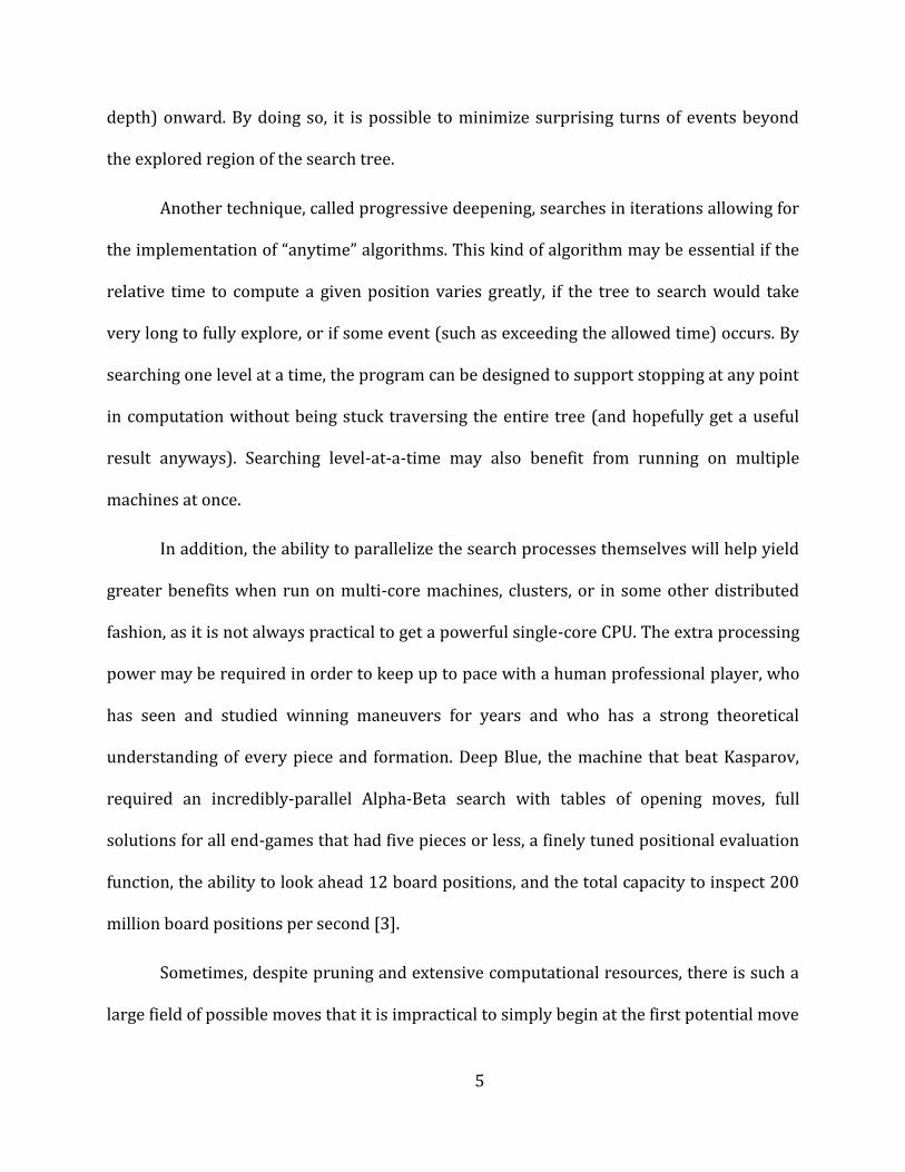
depth) onward. By doing so, it is possible to minimize surprising turns of events beyond
the explored region of the search tree.
Another technique, called progressive deepening, searches in iterations allowing for
the implementation of “anytime” algorithms. This kind of algorithm may be essential if the
relative time to compute a given position varies greatly, if the tree to search would take
very long to fully explore, or if some event (such as exceeding the allowed time) occurs. By
searching one level at a time, the program can be designed to support stopping at any point
in computation without being stuck traversing the entire tree (and hopefully get a useful
result anyways). Searching level-at-a-time may also benefit from running on multiple
machines at once.
In addition, the ability to parallelize the search processes themselves will help yield
greater benefits when run on multi-core machines, clusters, or in some other distributed
fashion, as it is not always practical to get a powerful single-core CPU. The extra processing
power may be required in order to keep up to pace with a human professional player, who
has seen and studied winning maneuvers for years and who has a strong theoretical
understanding of every piece and formation. Deep Blue, the machine that beat Kasparov,
required an incredibly-parallel Alpha-Beta search with tables of opening moves, full
solutions for all end-games that had five pieces or less, a finely tuned positional evaluation
function, the ability to look ahead 12 board positions, and the total capacity to inspect 200
million board positions per second [3].
Sometimes, despite pruning and extensive computational resources, there is such a
large field of possible moves that it is impractical to simply begin at the first potential move
6
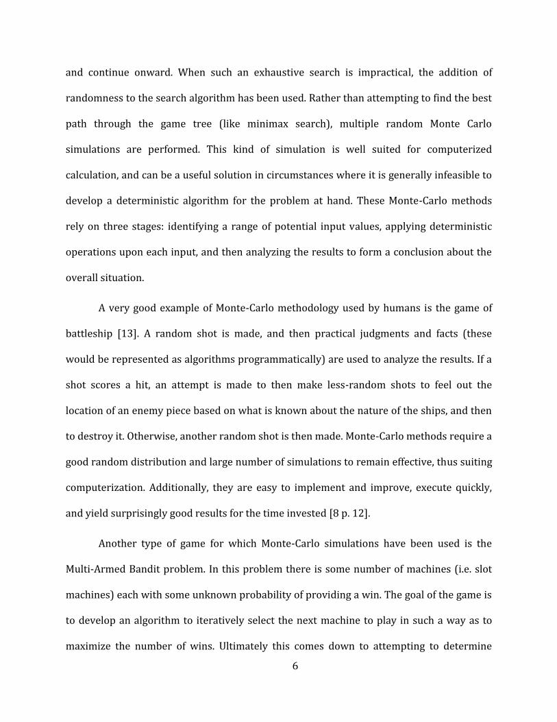
and continue onward. When such an exhaustive search is impractical, the addition of
randomness to the search algorithm has been used. Rather than attempting to find the best
path through the game tree (like minimax search), multiple random Monte Carlo
simulations are performed. This kind of simulation is well suited for computerized
calculation, and can be a useful solution in circumstances where it is generally infeasible to
develop a deterministic algorithm for the problem at hand. These Monte-Carlo methods
rely on three stages: identifying a range of potential input values, applying deterministic
operations upon each input, and then analyzing the results to form a conclusion about the
overall situation.
A very good example of Monte-Carlo methodology used by humans is the game of
battleship [13]. A random shot is made, and then practical judgments and facts (these
would be represented as algorithms programmatically) are used to analyze the results. If a
shot scores a hit, an attempt is made to then make less-random shots to feel out the
location of an enemy piece based on what is known about the nature of the ships, and then
to destroy it. Otherwise, another random shot is then made. Monte-Carlo methods require a
good random distribution and large number of simulations to remain effective, thus suiting
computerization. Additionally, they are easy to implement and improve, execute quickly,
and yield surprisingly good results for the time invested [8 p. 12].
Another type of game for which Monte-Carlo simulations have been used is the
Multi-Armed Bandit problem. In this problem there is some number of machines (i.e. slot
machines) each with some unknown probability of providing a win. The goal of the game is
to develop an algorithm to iteratively select the next machine to play in such a way as to
maximize the number of wins. Ultimately this comes down to attempting to determine
7
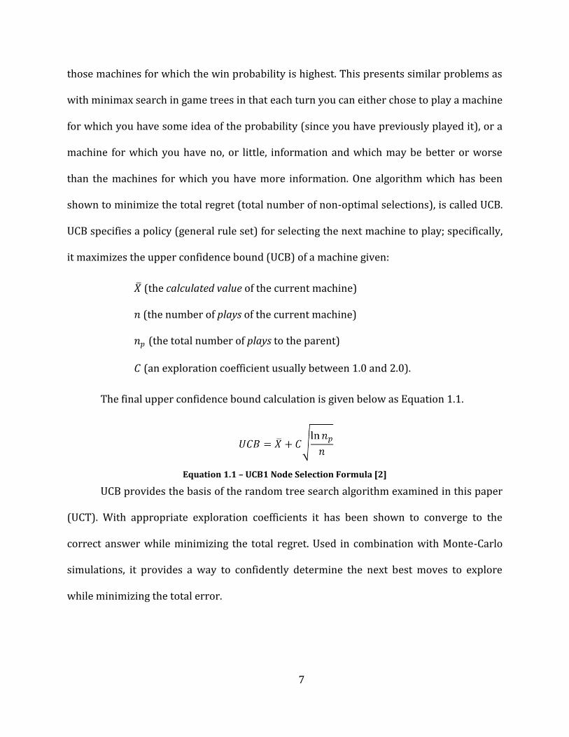
those machines for which the win probability is highest. This presents similar problems as
with minimax search in game trees in that each turn you can either chose to play a machine
for which you have some idea of the probability (since you have previously played it), or a
machine for which you have no, or little, information and which may be better or worse
than the machines for which you have more information. One algorithm which has been
shown to minimize the total regret (total number of non-optimal selections), is called UCB.
UCB specifies a policy (general rule set) for selecting the next machine to play; specifically,
it maximizes the upper confidence bound (UCB) of a machine given:
𝑋 (the calculated value of the current machine)
𝑛 (the number of plays of the current machine)
𝑛𝑝 (the total number of plays to the parent)
𝐶 (an exploration coefficient usually between 1.0 and 2.0).
The final upper confidence bound calculation is given below as Equation 1.1.
Equation 1.1 – UCB1 Node Selection Formula [2]
UCB provides the basis of the random tree search algorithm examined in this paper
(UCT). With appropriate exploration coefficients it has been shown to converge to the
correct answer while minimizing the total regret. Used in combination with Monte-Carlo
simulations, it provides a way to confidently determine the next best moves to explore
while minimizing the total error.
8
1.2 The Rules of Go
In order to understand the applications of random search algorithms to Go, it is first
important to understand the basic rules of the game. In Go, unlike chess, players begin with
no pieces on the board. Players alternate placing stones on the playing field as they
compete to secure territories by encircling areas by generally forming “chains” of pieces,
often capturing enemy pieces in the process. Pieces are fully captured and removed from
the board when the amount of liberties the piece has is reduced to zero; a liberty is the
number of free spaces present both to the piece in question, and to all friendly pieces that
make up the chain that piece belongs to. The rules and manner of playing pieces lead to the
possibility of arriving at certain board positions several times in several different ways,
which requires special consideration.
Victory does not require total board domination or focus on preparation for a
certain move that triggers game conclusion, but rather requires a player to go through
series of moves and counter-moves that are “good enough” at earning points for the
current play-through. A win by 0.5 positions, therefore, is just as valued a final goal as a win
by 87.5 (total domination on a 9x9 board). Identifying positions and strategies that are
useful, and those that should be abandoned or overlooked, is important. Essentially, Go is
well suited to human players who can easily handle the decisions required to a significant
depth while easily (and often passively) determining what possibilities or choices are
insignificant; computers are disadvantaged when it comes to these calculations. In
particular it is especially difficult for computers accurately disregard bad moves without
first devoting a certain amount of computational resources to determining if they are bad.
Humans, on the other hand, tend to be good at more quickly disregarding bad moves and
9
focusing in on a subset of the moves that are more likely to be successful. In a game of Go,
there is additionally the potential for moves to result in piece recaptures and extended
loops, both of which are restricted by the infinite-game avoiding rules of ko and superko,
respectively. Typically these moves are disallowed in most rule sets, although some rule
sets instead allow the move or consider it a forced loss for the player that makes the move.
Also unlike chess, the end of a match is not a certain, predictable event to be planned
for easily. The game generally concludes when both players opt to pass consecutively, each
believing to have either won decisively or believing that making a move would threaten
their strategy. A player who believes a win is impossible, even considering potential enemy
mistakes, may also opt to resign instead of just passing; this results in an automatic loss.
1.3 Algorithms for Go
Originally, Go was approached on smaller scales than what humans typically find
particularly challenging, namely on 9x9 boards. As with chess, programmers attempted to
use traditional min-max tree searching to evaluate moves, or attempted to use some table
of expert-based knowledge that would be processed. But with a typical branching factor of
about 200 compared to chess’ branching factor of 40, playing on a larger board would be
quite strenuous to the computer player, and require some new procedures. Interest in
developing better algorithms and tuning existing methods began around 1984, when
USENIX hosted the first computer Go competitions [6]. While the USENIX competition
ended in 1988, there have been competitions every year since, and there has been
continual development of computerized Go players.
10
A variety of different attempts have been made to compute a solution for Go,
through the use of traditional AI techniques that worked for chess, and search algorithms
such as minimax and Alpha-Beta. Due to the high branching factor of Go, as suggested
above, this is not particularly effective and has significant drawbacks as the board size
increases. The opening move selection, in particular, is a main source of challenge to Go-
playing programs. There also do not exist detailed opening-game and end-game tables for
Go as there do for chess, although a few programs do use some due to the difficulty of
establishing certain good opening moves via heuristics (it is much easier to have a list of
known strong openings and attempt to emulate them). GnuGo uses a variety of heuristics
designed to either strengthen or weaken other stones and determine the strategic value of
a play or portion of the board, in addition to determining the pure territorial value of the
board, for making generalizations about potential moves.
The use of hand-crafted “expert knowledge” systems has often been attempted
using pattern matching and rule-based systems. However, managing this kind of
information manually became increasingly difficult. Often, even good algorithms required a
certain degree of modification and tuning to get all the parameters for their search, move
comparison, and play selection algorithms operating efficiently. Partly because of this,
attempts were made to create programs that used artificial neural networks to learn, such
as NeuroGo [5] or Jellyfish. These still only competed on a typical “medium” level compared
to the other programs. Naturally, the various techniques developed have been mixed
together as well in an attempt to make up for the weaknesses of any particular method.
Beyond the algorithms that rely on known strategies, movement rules, and pattern
matching, however, there are also algorithms that rely on intentionally random
11
computation methods. In order to address the branching possibilities represented by every
round of Go, which are most often represented internally and conceptually as a tree,
Monte-Carlo randomized simulation came into use (although some programs rely more
heavily on pre-computed opening move tables for early-game simulation) in the early 90s;
due to their useful attributes, they are still used in current Go programs. Typically, these
Monte-Carlo simulations are used in a straightforward way when it comes to Go board
evaluation: first, random board positions (representing possible plays) are selected, and
then a series of sub-games branch off from there. The result is that many thousands of
these simulations are run to evaluate the probable outcome for the move, although the
selected play positions evaluated are not always optimal. The better the program is at
anticipating its own best moves (and what the resulting best moves for the opponent
should be), the more accurate the analysis of that particular board position. Naturally, the
more potential positions there are, the longer this analysis will take to compute. Most Go
programs, especially in tournament settings, are limited to the number of simulated sub-
games they can accomplish in a set period of time. Thus, more time dedicated to each
simulation will reduce the relative depth of the search possible. The standard method was
to uniformly sample actions, or attempt to heuristically bias the samplings (without
guaranteed results or appropriateness of those heuristics).
A method to selectively bias the Monte-Carlo simulations, for optimal evaluation and
use of processing, is required for the sensible selection of near-optimal moves. Due to the
large number of potential moves at every step of the game, a failure to optimize in this
fashion could result in searches that are too shallow to be conclusive; achieving
computational savings are important to accurate results. The use of bandit search
12
algorithms and methods for focusing the search would yield benefits by focusing on sets of
moves that are most promising.
Applying the multi-armed bandit algorithm, UCB, to trees yields the new algorithm
UCT (upper confidence bounding for trees), developed by Levente Kocsis and Csaba
Szepesvari of SZTAKI [11].
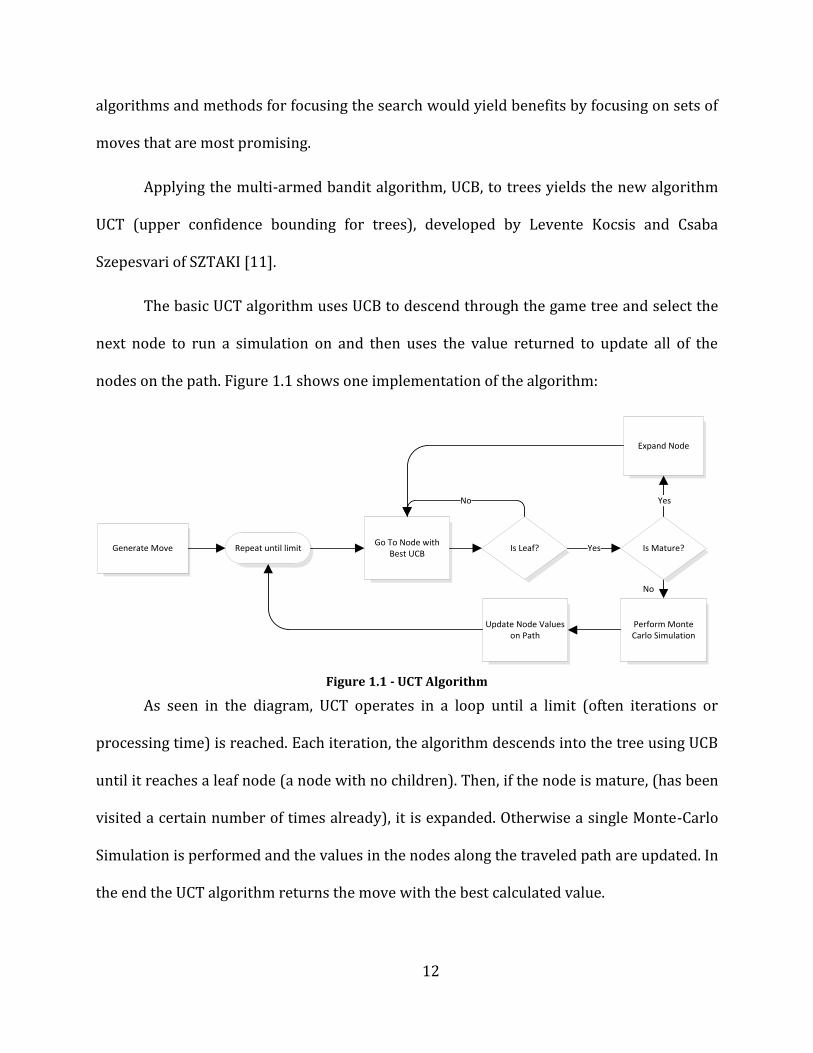
The basic UCT algorithm uses UCB to descend through the game tree and select the
next node to run a simulation on and then uses the value returned to update all of the
nodes on the path. Figure 1.1 shows one implementation of the algorithm:
Generate MoveGo To Node with
Best UCBIs Leaf?
No
Perform Monte Carlo Simulation
Yes
Update Node Values on Path
Repeat until limit
No
Is Mature?
Expand Node
Yes
Figure 1.1 - UCT Algorithm
As seen in the diagram, UCT operates in a loop until a limit (often iterations or
processing time) is reached. Each iteration, the algorithm descends into the tree using UCB
until it reaches a leaf node (a node with no children). Then, if the node is mature, (has been
visited a certain number of times already), it is expanded. Otherwise a single Monte-Carlo
Simulation is performed and the values in the nodes along the traveled path are updated. In
the end the UCT algorithm returns the move with the best calculated value.
13
UCT-based algorithms allow the Monte Carlo simulations to be focused on particular
areas of interest, where confidence in the moves is highest and the potential payoff for
investigation is optimal. This allows better use of Monte-Carlo simulation, as opposed to
simple, uniformly applied random sampling. UCT is able to analyze the likelihood of a
particular position being useful, and will only expand search tree nodes that reach a certain
threshold of examination during play-through. This generally limits the amount of
processing time wasted exploring unproductive moves. Compared to Alpha-Beta searching
as used in chess, UCT is much more efficient. It still produces good results even if stopped
early.
UCT also scales much better than other algorithms, requiring smaller sample sizes
to achieve the same rate of error. In experiments by Levente Kocsis and Csaba Szepesvari,
UCT was shown to perform well in simple Markovian games modeled as trees [11]. These
artificial game trees provided a basis for running UCT where it is possible to calculate the
exact answer ahead of time and thereby calculate the exact amount of error. This is unlike
simulations using Go, where it is impossible to calculate the exact best move in a timely
manner. The behavior of UCT on such artificial trees can provide some idea as to its
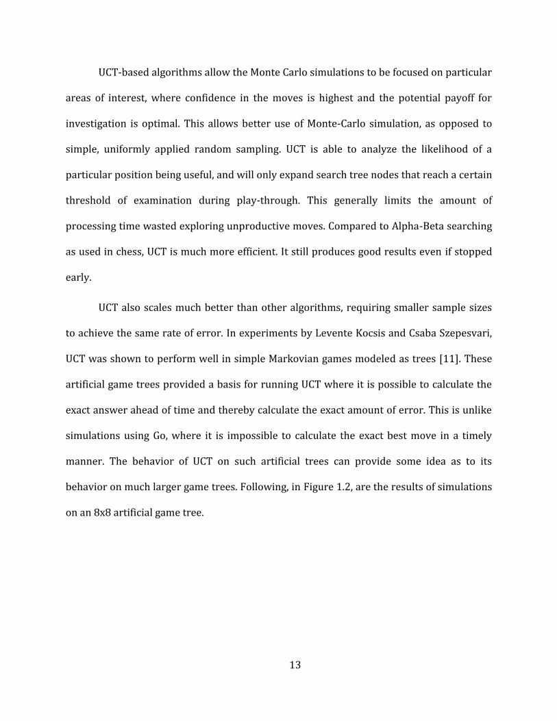
behavior on much larger game trees. Following, in Figure 1.2, are the results of simulations
on an 8x8 artificial game tree.
14
Figure 1.2 - UCT Experiment on Artificial Game Tree
Shown above is a logarithmic plot of the average error of selected moves versus the
number of iterations performed for both UCT and Alpha-Beta search. As seen above UCT
begins to approach zero error after less than 10,000 iterations. Alpha-Beta searching
results remain consistently poor until a sizable number of iterations have been performed,
after which it approaches zero error; unfortunately, however, it remains unusable for the
smaller series of iterations, and ends up converging to zero only past 10,000 iterations.
UCT’s ability to produce usable results so quickly makes it the obvious best choice of the
group.
Since UCT converges to the correct answer much sooner than Alpha-Beta, for the
same size tree, it can be applied to much larger-scale applications. This makes it useful in
Go, especially on the 13x13 and 19x19 boards where previous algorithms perform poorly.
In these situations it is important to sample the tree in such a way to balance the need to
explore new areas of the tree with the current best moves. This exploration-exploitation
problem is handled through the use of the UCB calculation with UCT. Often, there is not a
large amount of time provided to complete a detailed calculation of each outcome possible.
15
UCT, due to the lower number of samples required, can also be stopped sooner than other
algorithms while still giving useful results.
1.4 Investigations into UCT Enhancements
While UCT is capable of outperforming many prior algorithms that have been
developed, there is still much room for improvement. Only very recently has the computer-
go champion program MoGo been able to defeat a skilled player on a 9x9 board [10]. Two
main areas of investigation are modifications to UCB/UCT itself, and the introduction of
grouping nodes to the tree.
1.4.1 UCB Modifications
UCB itself has been experimented with in a variety of ways. Auer et al investigated
the behavior of several tweaks including UCB1-Tuned, UCB2, and GREEDY [2]. The first
variant, known as UCB1-Tuned, is identical aside from a modified upper confidence bound.
It performs better, compared to the original, when dealing with varied and non-optimal
scenarios. UCB2, another version, performs as a degraded UCB1-tuned, although it operates
relatively insensitively to the alpha-value of the UCB algorithm as long as it is kept small (to
the order of 0.001). Another variant similar to UCB1-Tuned, known as GREEDY, explores
uniformly but requires tuning for each application in order to perform well. Another
modification for UCB was examined in BAST, the Bandit Algorithm for Smooth Trees, also
introduces the concept of tree smoothness [4]. Coquelin and Munos showed a particular
case where UCT performed poorly and suggested the addition of a smoothness constant
which would alter UCT’s behavior to be more pessimistic in the exploration of tree.
16
1.4.2 MOGO
The current champion Go program, MoGo became the first Go program to use UCT,
in July 2006, very shortly after UCT’s publication. It was developed as a closed-source
project at the Laboratoire de Recherche en Informatique in France, but after the original
author completed his studies other students took over MoGo development (its source code
is still not publicly available, however). Since its first KGS international Go tournament win
(9x9 and 13x3) in August of 2006, it has been awarded much recognition for its
performance, including several computer-go championship wins [7]. UCT, in MoGo, has
been augmented and adjusted in a number of different ways to improve its performance.
For example, it combines the implementation of UCT with a database of opening moves, as
the openings are the hardest part of the game for a computerized player to analyze. This
gives it an edge during the early game and provides several different strategies to choose
from, while still allowing for UCT to augment its move selection in the later game to ensure
victory. It also compensates for the tendency of Monte-Carlo simulation to be relatively
inaccurate for early board positions or situations where the game would go on for a very
long [8 p. 11]. Mogo has also worked to improve the simulation portion of UCT where
rather than using completely random simulations, a more realistic, heuristic based,
simulation is used. This serves to provide more accurate results from the Monte-Carlo
simulations and has been seen to provide significant improvements over purely random
simulations.
In addition, several groups, including the one behind MoGo, have experimented with
parallelization of the UCT process [8 p. 53]. The result is more simulations per second and
thus greater accuracy for the simulation process. Potential options include optimizations
17
for shared-memory multi-processor computation on a single machine, and changes that
will better support distributed computing operation on a cluster. Currently, Windows ports
of MoGo may perform more slowly than other versions as they do not support multi-
processor systems. Unfortunately, however, initial investigations have shown that the
potential for speedups under a cluster situation is not as good as the speedups found on a
single machine with multiple processors. In fact, it may even perform worse in some
circumstances without nontrivial modification [15 p. 2].
1.4.3 Directed Acyclic Graphs
Current Go algorithms that use UCT generally operate on the game as if it were a
tree. However, as mentioned previously, in the game of Go, and many other similar games,
it is quite possible to reach the same board position with several different move orderings.
Thus while the tree representation will be accurate, some sections of the tree will be
duplicates. In fact for any one duplicated board position all subsequent board positions in
the tree will be duplicated as well. Thus a duplicate position close to the top of the tree will
result in a significant number of extra nodes to be searched by UCT. Due to the rules of Go
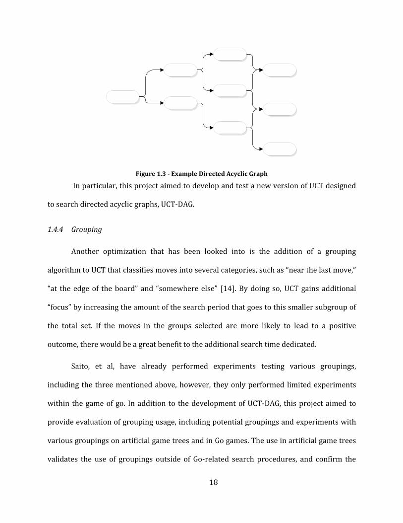
preventing cycles, directed acyclic graphs can be used to fix this inefficiency. Directed
acyclic graphs are essentially trees except instead of each node having a single parent,
nodes may have multiple parents. However, there may not be any cycles in the graph; an
example follows in Figure 1.3.
18
Figure 1.3 - Example Directed Acyclic Graph
In particular, this project aimed to develop and test a new version of UCT designed
to search directed acyclic graphs, UCT-DAG.
1.4.4 Grouping
Another optimization that has been looked into is the addition of a grouping
algorithm to UCT that classifies moves into several categories, such as “near the last move,”
“at the edge of the board” and “somewhere else” [14]. By doing so, UCT gains additional
“focus” by increasing the amount of the search period that goes to this smaller subgroup of
the total set. If the moves in the groups selected are more likely to lead to a positive
outcome, there would be a great benefit to the additional search time dedicated.
Saito, et al, have already performed experiments testing various groupings,
including the three mentioned above, however, they only performed limited experiments
within the game of go. In addition to the development of UCT-DAG, this project aimed to
provide evaluation of grouping usage, including potential groupings and experiments with
various groupings on artificial game trees and in Go games. The use in artificial game trees
validates the use of groupings outside of Go-related search procedures, and confirm the
19
benefit of implementing them within an environment more controlled and faster to process
than a game of Go.
The introduction of grouping into UCT has the potential to increase the number of
moves which can be visited from alternate paths. While Saito et al. looked at independent
groups (each move could be a member of only one group) [14], it is quite plausible that
groupings could be overlapping. In this case the game representation becomes much more
like a directed acyclic graph than a tree and the advantages of using an algorithm for
directed acyclic graphs may become more pronounced.
1.5 Conclusion
Since UCT was first published in 2006, [11], several groups have implemented and
improved upon the initial algorithm. With MoGo’s improvements this algorithm is now able
to be competitive with human experts on a 9x9 board. However, more work still needs to
be done in order to compete on larger boards. The fundamental issue that must be dealt
with on larger boards is an increased branching factor. By investigating the use of directed
acyclic graphs and grouping, this project aims to improve UCT’s performance on larger
boards. The primary focus of this project is in simulation and experimentation with the
proposed improvements. In order to show quantifiable results while remaining relevant to
the application of Go, simulations were performed both with games of Go using GnuGo, a
freely available opponent, and as an extension to the simulations on artificial game trees
originally used by our local coordinator Levente Kocsis at SZTAKI. The design and
development of these modifications are explored in the next chapter.

20
Chapter 2: Development
In order to test the effect of directed acyclic graphs and grouping on UCT, it was first
necessary to design and add this functionality to existing codebases that implemented UCT
on trees without grouping. We used two packages; first, the artificial game trees
experiment that Kocsis used in his initial papers (PGame) was used as a basis for
experiments on artificial game trees. Second, a publicly available package, LibEGO1 (Library
for Effective Go Routines), was also updated. In this chapter, implementation details of the
pre-existing codebases, the high level designs of these two features, and the details of
implementation within both codebases are explored.
2.1 Details of Existing Codebases
In the process of designing and developing the improvements for PGame and
LibEGO, it was necessary to understand the existing codebases. In this manner we could
thus determine the best course for implementing our changes. In the following two sections
some of the more important design details of PGame and LibEGO are presented in order to
illuminate some of the design decisions we made for our improvements.
2.1.1 PGame
PGame was originally written by Levente Kocsis as part of his initial paper on UCT.
It was designed to run UCT as well as Alpha Beta search and a simplistic Monte Carlo
Search on artificial game trees and then compile the results and compute some statistics on
the results. In order to implement our changes to PGame we primarily needed to modify
1 In its original form at http://www.mimuw.edu.pl/~lew/hg/libego/?shortlog
21
the structure of the game tree to become a DAG with grouping. Thus it was important to
understand the initial structure of the game trees before designing our own
implementation.
The PGame artificial game trees represent a very simple game. Both players start
with a score of 0. In turn they both select a move which awards them a certain number of
points. This move moves to the next point in the tree where the next player can then select
from the available moves at that point. At the end the player with the most points wins the
game. Thus the goal of each player is to find the move that maximizes their score while
minimizing the score for their opponent. This simple tree structure presents some
challenges when attempting to convert it to a DAG. Primarily it is important to ensure that
the aggregate scores of the players are the same no matter which path is followed towards
a node. In order to ensure that this is the case, additional precautions must be taken in the
DAG generation algorithm.
In addition to the tree generation design, it is also important to understand the UCT
implementation itself. In PGame, UCT is implemented in a very simple manner. In each
iteration the algorithm selects the next node in the tree to move to. If no information exists
for the nodes, a random node is selected2. Otherwise the node with the highest UCB is
visited. Then, when the bottom of the tree is reached, all of the nodes along the tree path
are updated with the result (win/loss). This causes the Monte-Carlo simulations and UCB
descent to be integrated together rather than being separated in two phases. However, this
2 Note: Experiments have been performed (specifically with MoGo) in improving UCT’s performance
by improving the Monte-Carlo simulations with a heuristic based search. This has proven successful, however as it is already well known we did not re-implement such improvements in this project.

22
fact does not materially affect the implementation of the grouping or UCT-DAG algorithms
as they focus primarily on differences in the tree generation algorithm.
2.1.2 LibEGO
Unlike the PGame experiments, much of the design and development work with
LibEGO focused on the UCT algorithm itself as the game generation was set by the rules of
Go. One important difference in the LibEGO implementation of UCT is that the Monte-Carlo
simulations were separated from the UCB descent. This was necessary due to the fact that
storing each move for all of the many play outs would require an unmanageable amount of
memory. In order to solve this problem, LibEGO introduced the concept of node maturity
where a node in the UCT tree would not be expanded until a certain number of Monte-Carlo
simulations had been performed. After each simulation, the moves selected would be
discarded and the UCT tree would be updated with the result. In this way the size of the
tree is limited.
LibEGO also used many very compact and complex data structures in an effort to
increase performance and decrease memory usage. Thus it provided somewhat of a
challenge to implement our features within the existing data structures while minimizing
the changes in memory usage and performance. The tree structure had to be modified in
order to support DAG’s, especially with regards to memory management. We had to
implement reference counting on tree nodes so that they would be deleted when they are
no longer referenced, not when one of their parents are deleted as was the case with the
initial implementation. In the next sections we describe the actual design and
implementation of our features within both PGame and LibEGO.
23
2.2 UCT on Directed Acyclic Graphs
As discussed in section 1.4.3, directed acyclic graphs (DAGs) can be used as a means
for reducing the size of the search space. However, in order to use UCT on DAGs, an
algorithm designed for use on trees, some modifications must be made. The original UCT
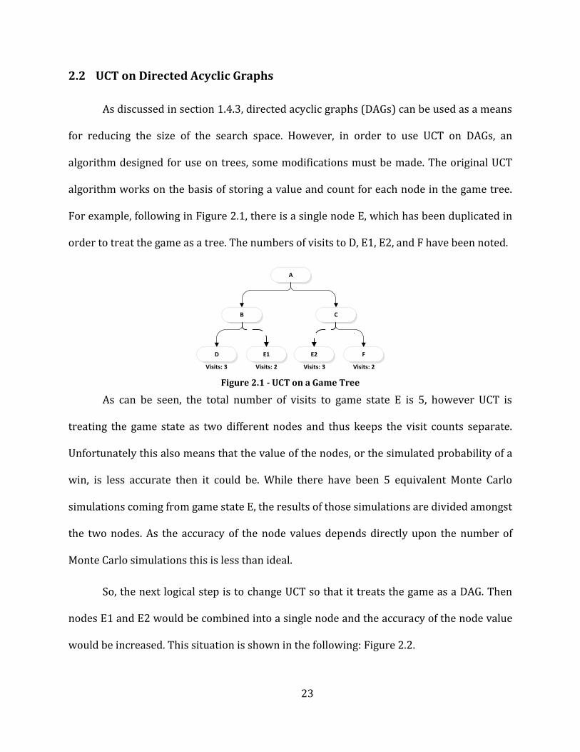
algorithm works on the basis of storing a value and count for each node in the game tree.
For example, following in Figure 2.1, there is a single node E, which has been duplicated in
order to treat the game as a tree. The numbers of visits to D, E1, E2, and F have been noted.
A
B C
D E1 F
`
Visits: 3 Visits: 2 Visits: 2
E2
Visits: 3
Figure 2.1 - UCT on a Game Tree
As can be seen, the total number of visits to game state E is 5, however UCT is
treating the game state as two different nodes and thus keeps the visit counts separate.
Unfortunately this also means that the value of the nodes, or the simulated probability of a
win, is less accurate then it could be. While there have been 5 equivalent Monte Carlo
simulations coming from game state E, the results of those simulations are divided amongst
the two nodes. As the accuracy of the node values depends directly upon the number of
Monte Carlo simulations this is less than ideal.
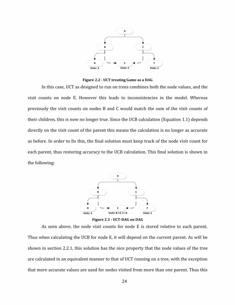
So, the next logical step is to change UCT so that it treats the game as a DAG. Then
nodes E1 and E2 would be combined into a single node and the accuracy of the node value
would be increased. This situation is shown in the following: Figure 2.2.
24
A
B C
D E F
`
Visits: 3 Visits: 5 Visits: 2
Figure 2.2 - UCT treating Game as a DAG
In this case, UCT as designed to run on trees combines both the node values, and the
visit counts on node E. However this leads to inconsistencies in the model. Whereas
previously the visit counts on nodes B and C would match the sum of the visit counts of
their children, this is now no longer true. Since the UCB calculation (Equation 1.1) depends
directly on the visit count of the parent this means the calculation is no longer as accurate
as before. In order to fix this, the final solution must keep track of the node visit count for
each parent, thus restoring accuracy to the UCB calculation. This final solution is shown in
the following:
A
B C
D E F
`
Visits: 3 Visits: B->2, C->3 Visits: 2
Figure 2.3 - UCT-DAG on DAG
As seen above, the node visit counts for node E is stored relative to each parent.
Thus when calculating the UCB for node E, it will depend on the current parent. As will be
shown in section 2.2.1, this solution has the nice property that the node values of the tree
are calculated in an equivalent manner to that of UCT running on a tree, with the exception
that more accurate values are used for nodes visited from more than one parent. Thus this

25
change serves only to increase the accuracy of node values without jeopardizing the
accuracy of UCB calculations or changing the exploration and exploitation properties of
UCT which make it so successful.
We also considered additional methods for updating UCT to perform well on DAGs.
One immediate thought is to somehow update nodes on paths other than the path taken to
a node with the latest value after a single iteration. For instance, if UCT was run for a single
additional iteration on the DAG in Figure 2.3, it might take the path A->B->E, it would then
perform a Monte-Carlo simulation and update the values on nodes E,B and A. However, this
simulation should also be valid for node C. Thus it would be interesting to consider how to
update C in such a way as to maintain the accuracy of the values on all the nodes.
Unfortunately this is not entirely obvious and is complicated in cases where there are
multiple paths back to a single parent. It is also important to consider the performance
implications of such updating. Depending on the complexity of the DAG, it is possible that
the number of ancestors to be updated could be very large, potentially exponential. Due to
these complexities and the time constraints of this project, we were unable to satisfactorily
investigate this possibility. Instead we focused on UCT-DAG, which provides a small change
that is relatively straightforward to implement and has minimal performance impact.
2.2.1 Behavior of UCT-DAG
One of the primary goals in adapting UCT to directed acyclic graphs was to ensure
that the algorithm continued to behave in the way described in its original form. In Kocsis’s
original paper on the topic, he showed that UCT converges to the correct answer and that
the expected error rate decreases as the number of iterations increases [11]. A core part of
26
this proof is the statistical behavior of the upper confidence bound. As the number of
samples (Monte Carlo Simulations) increases, so does the accuracy of the calculated value,
thus the confidence interval (within which the actual value lies with specified probability),
becomes smaller. The primary aim of UCT-DAG is to improve the accuracy of the calculated
values by sharing the results of Monte Carlo Simulations between identical nodes, while
retaining the statistical validity of the upper confidence bound.
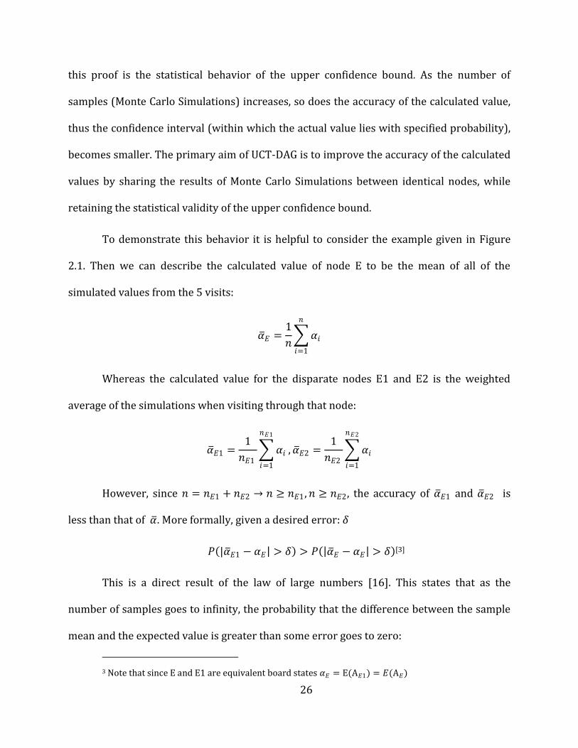
To demonstrate this behavior it is helpful to consider the example given in Figure
2.1. Then we can describe the calculated value of node E to be the mean of all of the
simulated values from the 5 visits:
𝛼 𝐸 =1
𝑛 𝛼𝑖
𝑛
𝑖=1
Whereas the calculated value for the disparate nodes E1 and E2 is the weighted
average of the simulations when visiting through that node:
𝛼 𝐸1 =1
𝑛𝐸1 𝛼𝑖
𝑛𝐸1
𝑖=1
, 𝛼 𝐸2 =1
𝑛𝐸2 𝛼𝑖
𝑛𝐸2
𝑖=1
However, since 𝑛 = 𝑛𝐸1 + 𝑛𝐸2 → 𝑛 ≥ 𝑛𝐸1 , 𝑛 ≥ 𝑛𝐸2, the accuracy of 𝛼 𝐸1 and 𝛼 𝐸2 is
less than that of 𝛼 . More formally, given a desired error: 𝛿
𝑃 |𝛼 𝐸1 − 𝛼𝐸 > 𝛿 > 𝑃 𝛼 𝐸 − 𝛼𝐸 > 𝛿 [3]
This is a direct result of the law of large numbers [16]. This states that as the
number of samples goes to infinity, the probability that the difference between the sample
mean and the expected value is greater than some error goes to zero:
3 Note that since E and E1 are equivalent board states 𝛼𝐸 = E(Α𝐸1) = 𝐸(Α𝐸)
27
lim𝑛→∞
𝑃 𝑋 𝑛 − 𝐸 𝑋 > 𝛿 = 0
Next one must consider how sharing the values between E1 and E2 will affect the
values and accuracy of the parent calculations. With UCT the values of the parent nodes and
the counts of the parent nodes could be calculated as a weighted average of the child values
and counts. So in the case of node B:
𝑛𝑏 = 𝑛𝑑 + 𝑛𝐸1, 𝛼 𝐵 =1
𝑛𝑏⋅ 𝑛𝑑 ⋅ 𝛼 𝐷 + 𝑛𝐸1 ⋅ 𝛼 𝐸1
With the proposed UCT-DAG modification this changes very slightly to become:
𝑛𝑏 = 𝑛𝑑 + 𝑛𝐸1 , 𝛼 𝐵(𝐷𝐴𝐺) =1
𝑛𝑏⋅ 𝑛𝑑 ⋅ 𝛼 𝐷 + 𝑛𝐸1 ⋅ 𝛼 𝐸
Thus the only difference is to use a more accurate estimation of value for node E.
Thus the accuracy of the modified 𝛼 𝐵 is better than the accuracy of the original estimate
and:
𝑃 |𝛼 𝐵 − 𝛼𝐵 > 𝛿 > 𝑃(|𝛼 𝐵(𝐷𝐴𝐺) − 𝛼𝐵| > 𝛿)
It should be noted that since the counts are kept per parent rather than per node,
the UCB calculations when descending the tree will actually be more pessimistic than they
actually must be. In the previous example, for instance, node B would calculate the upper
confidence bound of node E using the visit count of 3, which would result in a higher upper
confidence bound than if it used the actual visit count of 5. However due to the
inconsistencies noted above regarding the use of aggregate counts for nodes rather than
counts per parent, it is not trivial exactly how to deal with this pessimism. It is important to
note that even with this additional pessimism, UCT-DAG is operating with more accurate
28
information than is available in plain UCT. Thus its results will only be improved. It is
possible, however, that additional modifications could be made to further improve UCT-
DAG taking into account the aggregate counts at nodes. This, however, is left to future
research.
2.2.2 Transposition Table
One component of developing UCT-DAG involved the use of a transposition table to
store information by game state without regard to turn number or the path leading to the
state. Transposition tables are hash tables, which index some information by game state.
After performing the Monte Carlo simulations for a leaf, the node count instead of value
would be kept for the current path, with the value of the current board position instead
updated in the transposition table. This use of transposition tables with UCT-DAG is quite
convenient as it allows an existing tree representation to remain in place while still sharing
information between duplicate nodes. In addition it is possible to save the transposition
table between moves further improving the accuracy of UCT as existing simulation results
may be reused in the next search.
2.3 UCT-DAG Implementation
The implementation of UCT-DAG both on Artificial Game Trees as well as in LibEGO
required specific modifications in order to work within the pre-existing codebase. Details
of these modifications are given in the following sections.
29
2.3.1 PGame
Implementing UCT-DAG on artificial game trees required two steps. First the game
generation procedure had to be modified to generate a DAG rather than a Tree. Next the
UCT algorithm had to be updated to store node visit counts separately for each parent as
discussed in section 2.2.
In order to add support for DAGs to PGame the data structures had to be modified.
The tree implementation used a simple array to store tree nodes and links between nodes
were implicitly defined by the branching factor and depth of the tree. In this structure, the
root is stored in the first position of the array; the children at the next level are stored in
the next positions, and so on. To support a DAG, this structure had to be modified such that
each node also stored links to its children. This was necessary as in a DAG, there are not a
fixed number of nodes at any level and thus it is impossible to directly compute the indices
of a node’s children given the depth and breadth of the DAG. In addition each node now
needed to store the values of a move to each of its children. The move value was previously
stored in the node itself (since it had only one parent), but now, this information needed to
be stored in the parent node.
In addition, the generation procedure itself needed to be modified. In the previous
version the only generation step was to generate random move values for each node in the
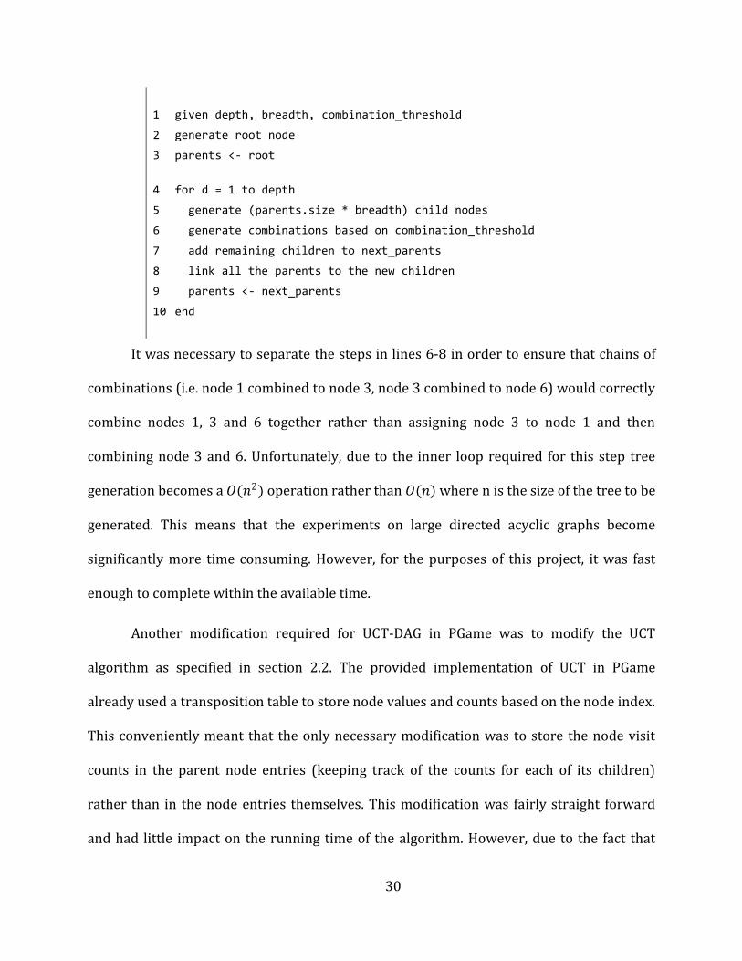
tree. Generating a DAG, however required a multi-step process shown in pseudo-code
below:
30
1 given depth, breadth, combination_threshold
2 generate root node
3 parents <- root
4 for d = 1 to depth
5 generate (parents.size * breadth) child nodes
6 generate combinations based on combination_threshold
7 add remaining children to next_parents
8 link all the parents to the new children
9 parents <- next_parents
10 end
It was necessary to separate the steps in lines 6-8 in order to ensure that chains of
combinations (i.e. node 1 combined to node 3, node 3 combined to node 6) would correctly
combine nodes 1, 3 and 6 together rather than assigning node 3 to node 1 and then
combining node 3 and 6. Unfortunately, due to the inner loop required for this step tree
generation becomes a 𝑂(𝑛2) operation rather than 𝑂(𝑛) where n is the size of the tree to be
generated. This means that the experiments on large directed acyclic graphs become
significantly more time consuming. However, for the purposes of this project, it was fast
enough to complete within the available time.
Another modification required for UCT-DAG in PGame was to modify the UCT
algorithm as specified in section 2.2. The provided implementation of UCT in PGame
already used a transposition table to store node values and counts based on the node index.
This conveniently meant that the only necessary modification was to store the node visit
counts in the parent node entries (keeping track of the counts for each of its children)
rather than in the node entries themselves. This modification was fairly straight forward
and had little impact on the running time of the algorithm. However, due to the fact that
31
PGame’s UCT used a transposition table to store node values and counts, it exhibited
behavior similar to the second example given in section 2.2, where UCT was running on a
DAG (sharing node counts and values between nodes). Thus a final modification was
necessary where functionality was added to convert a DAG into a tree (duplicating nodes),
in order to test UCT running on a tree, but with duplicate nodes.
With support for UCT-DAG completed, the next step was to run experiments
comparing its performance with UCT. With a parameter to control the number of nodes
with multiple parents, the performance could be compared with different levels of overlap.
2.3.2 LibEGO
In order to support UCT-DAG in LibEGO, some major changes needed to be made in
terms of the way node values and counts were stored in memory. In order to keep the
changes minimal, the in memory model of the UCT game was kept as a tree instead of as a
DAG, but duplicate nodes kept references into a transposition table in order to share the
node value. Node counts were kept in the nodes themselves.
32
Generate MoveGo To Node with
Best UCBIs Leaf?
No
Perform Monte Carlo Simulation
Yes
Update Node Count on Path
Repeat until limit
Transposition Table
Retrieve Board Position Value
Update Board Position Value, Count
No
Is Mature?
Expand Node
Yes
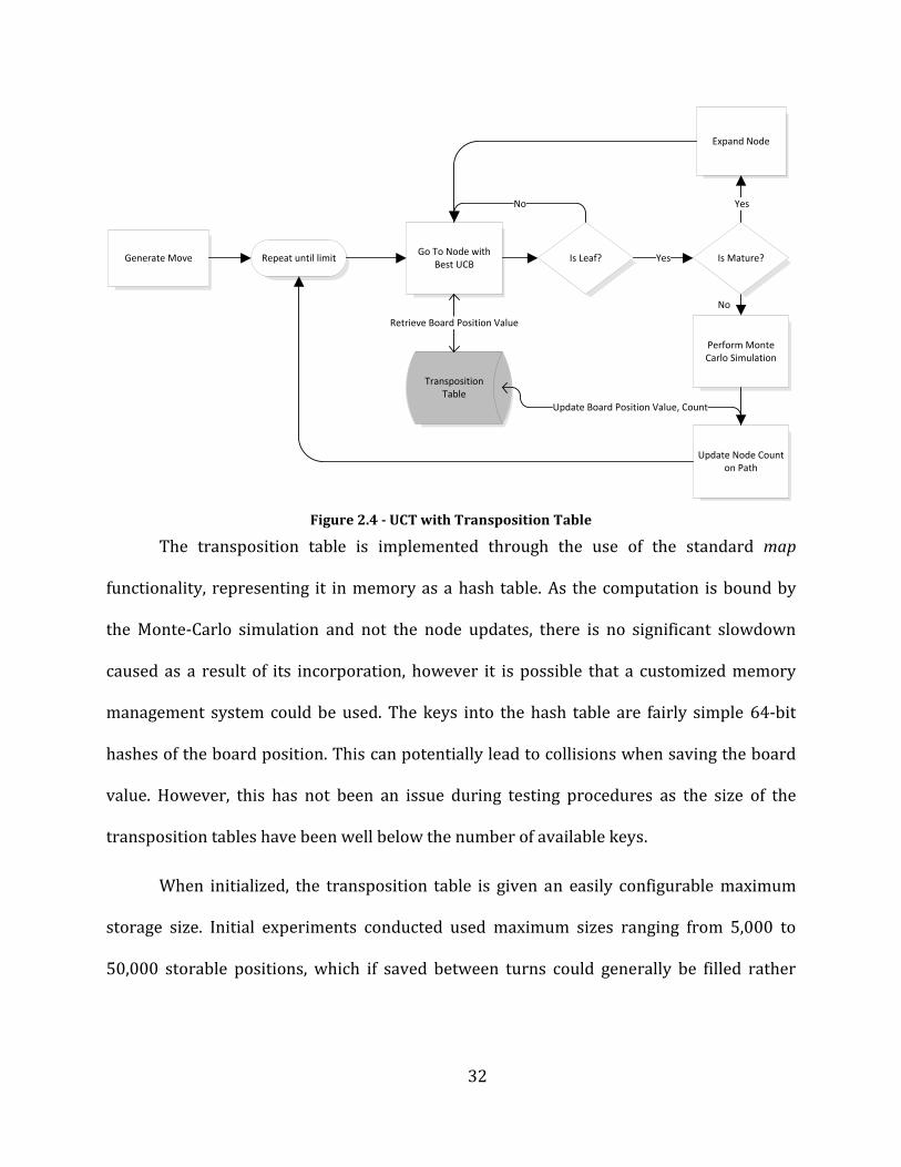
Figure 2.4 - UCT with Transposition Table
The transposition table is implemented through the use of the standard map
functionality, representing it in memory as a hash table. As the computation is bound by
the Monte-Carlo simulation and not the node updates, there is no significant slowdown
caused as a result of its incorporation, however it is possible that a customized memory
management system could be used. The keys into the hash table are fairly simple 64-bit
hashes of the board position. This can potentially lead to collisions when saving the board
value. However, this has not been an issue during testing procedures as the size of the
transposition tables have been well below the number of available keys.
When initialized, the transposition table is given an easily configurable maximum
storage size. Initial experiments conducted used maximum sizes ranging from 5,000 to
50,000 storable positions, which if saved between turns could generally be filled rather
33
quickly, often within the first three moves. The transposition table size worked comfortably
with up to 500,000 entries, although it could potentially go larger.
As the transposition table fills, data is stored in a first-come, first served manner.
During the opening moves of a typical game of Go, the average node parents that attempted
to inspect the same position appeared to typically stay around 1.85, or just under two. In
order to compensate for the table filling quickly with meaningless data, a system to “age”
the stored board positions was implemented, although it proved to be a source for error
more than a source for improved performance. When storing positional data between
moves, however, it was important to maintain only relevant data while pruning less-
frequently accessed information. Storing positional data between moves allows the useful
work that had been done during the last turn to be re-used, to allow for greater accuracy;
but it also fills up the transposition table faster, as each turn begins with a partially full
table instead of a blank one.
In order to prune the transposition table, a minimum threshold for position data
access was implemented, initialized to two (although easily configurable) based on early
observations. This meant that if less than two attempts were made to reference the
positional data, the data would be discarded instead of passed on during the next turn.
During the turn, the transposition table could potentially exceed the maximum storage size.
If this becomes the case, the minimum threshold is incremented, resulting in only the most
useful of the stored data being passed on. After the next turn, the increased threshold will
ensure that the transposition table is kept below its intended maximum size.
34
2.4 Grouping
The second improvement to UCT that we examined was grouping. The concept of
grouping in UCT, as discussed previously, had not been extensively explored. In addition,
the use of many groups adds significant overhead by increasing the number of nodes and
the depth of the search tree. Grouping introduces a new level of nodes in the graph, group
nodes, which evenly4 divide UCT-DAG’s attention into several sub-trees. In our
implementation, group overlap is allowed to occur, which will take advantage of the
transposition table. In fact, a default group that is provided when grouping is enabled
contains every node for consideration; thus, using any groups implies overlap in at least
one category automatically.
The alleged benefit of grouping is that large subsets of the node pool can be classed
into different categories, which can then be evaluated both on the node level and group
level. This allows entire groups to be considered potentially winning/beneficial, or
losing/undesirable. Because of this, purposely selecting only groups that are expected to be
consistently successful is not required; however, groups must generally correlate with
either winning or losing moves.
A
Group 1 Ungrouped
B (Win) C (Lose) D (Lose) E (Lose)
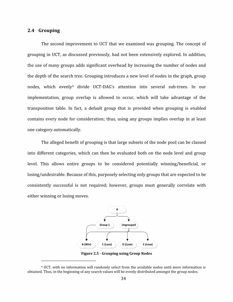
Figure 2.5 - Grouping using Group Nodes
4 UCT, with no information will randomly select from the available nodes until more information is
obtained. Thus, in the beginning of any search values will be evenly distributed amongst the group nodes.
35
In the above example, node A (with children B, C, D, E) was the start of the search
tree. During evaluation of its children, it was found that node B (the start of a series of
moves leading to a win) belonged to Group 1. Also during this process all nodes were found
to be members of the all-encompassing group. If there were no groups at work at all, until
enough simulations were calculated, each child would be given 25% of the time available.
As a result of the groups, UCT will spreading time first evenly among group nodes, the two
group nodes would receive 50% of the available processing. This leads to node B receiving
50% through being the only Group 1 node, and leads to nodes B, C, D and E receiving
another quarter each of the remaining 50%. In addition, after a number of simulations have
been performed, UCT will determine that Group 1 is the most likely winning group and will
devote even more time to exploring B and its children.
2.5 Grouping Implementation
In order to add grouping to both PGame and LibEGO, the games’ models needed to
be modified such that nodes could exist that represented groups rather than moves.
Additionally, the order of play had to be modified such that a player would choose a group
and a move each turn rather than just a move. This led to varying degrees of complication
with each implementation and was handled differently in both cases. Regardless, while the
overall goals were the same, in PGame it was necessary to invent an artificial grouping with
variable correlation to winning or losing moves, whereas with LibEGO it was necessary to
build a framework that allowed different grouping to be experimented with and specified
at runtime. The details of these modifications and the challenges presented by each are
detailed in the following sections.
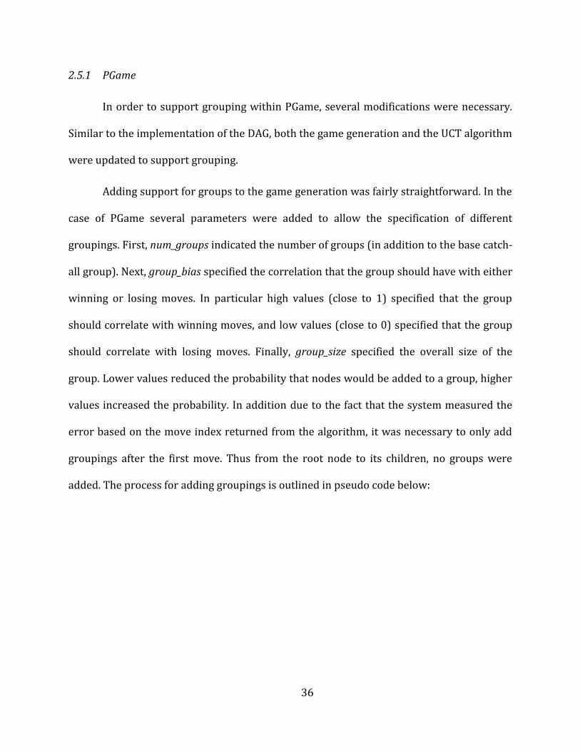
36
2.5.1 PGame
In order to support grouping within PGame, several modifications were necessary.
Similar to the implementation of the DAG, both the game generation and the UCT algorithm
were updated to support grouping.
Adding support for groups to the game generation was fairly straightforward. In the
case of PGame several parameters were added to allow the specification of different
groupings. First, num_groups indicated the number of groups (in addition to the base catch-
all group). Next, group_bias specified the correlation that the group should have with either
winning or losing moves. In particular high values (close to 1) specified that the group
should correlate with winning moves, and low values (close to 0) specified that the group
should correlate with losing moves. Finally, group_size specified the overall size of the
group. Lower values reduced the probability that nodes would be added to a group, higher
values increased the probability. In addition due to the fact that the system measured the
error based on the move index returned from the algorithm, it was necessary to only add
groupings after the first move. Thus from the root node to its children, no groups were
added. The process for adding groupings is outlined in pseudo code below:
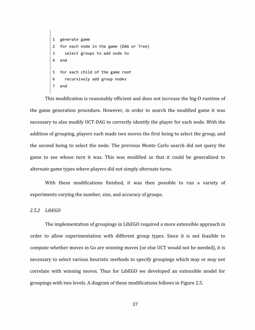
37
1 generate game
2 for each node in the game (DAG or Tree)
3 select groups to add node to
4 end
5 for each child of the game root
6 recursively add group nodes
7 end
This modification is reasonably efficient and does not increase the big-O runtime of
the game generation procedure. However, in order to search the modified game it was
necessary to also modify UCT-DAG to correctly identify the player for each node. With the
addition of grouping, players each made two moves the first being to select the group, and
the second being to select the node. The previous Monte Carlo search did not query the
game to see whose turn it was. This was modified so that it could be generalized to
alternate game types where players did not simply alternate turns.
With these modifications finished, it was then possible to run a variety of
experiments varying the number, size, and accuracy of groups.
2.5.2 LibEGO
The implementation of groupings in LibEGO required a more extensible approach in
order to allow experimentation with different group types. Since it is not feasible to
compute whether moves in Go are winning moves (or else UCT would not be needed), it is
necessary to select various heuristic methods to specify groupings which may or may not
correlate with winning moves. Thus for LibEGO we developed an extensible model for
groupings with two levels. A diagram of these modifications follows in Figure 2.5.
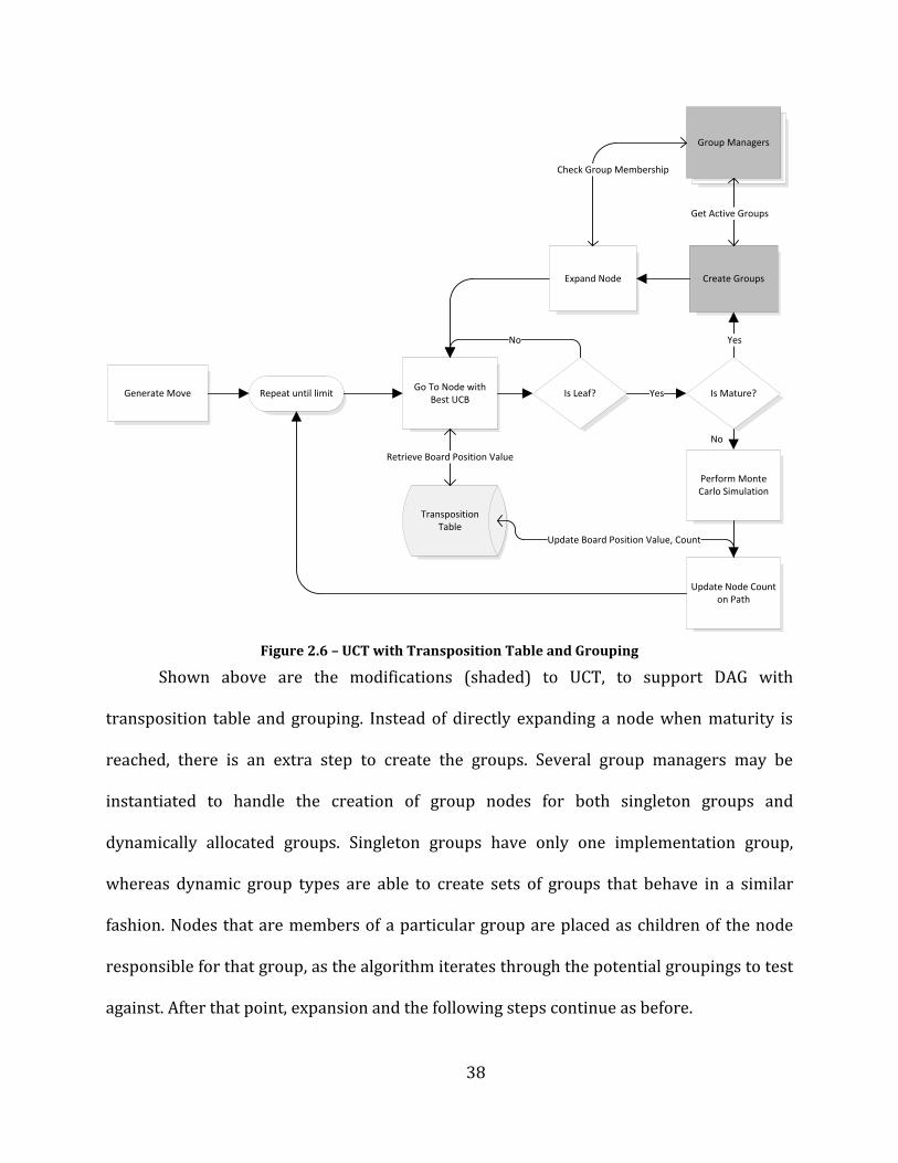
38
Generate MoveGo To Node with
Best UCBIs Leaf?
No
Perform Monte Carlo Simulation
Yes
Update Node Count on Path
Repeat until limit
Transposition Table
Retrieve Board Position Value
Update Board Position Value, Count
No
Is Mature?
Create Groups
Yes
Group Managers
Get Active Groups
Expand Node
Check Group Membership
Figure 2.6 – UCT with Transposition Table and Grouping
Shown above are the modifications (shaded) to UCT, to support DAG with
transposition table and grouping. Instead of directly expanding a node when maturity is
reached, there is an extra step to create the groups. Several group managers may be
instantiated to handle the creation of group nodes for both singleton groups and
dynamically allocated groups. Singleton groups have only one implementation group,
whereas dynamic group types are able to create sets of groups that behave in a similar
fashion. Nodes that are members of a particular group are placed as children of the node
responsible for that group, as the algorithm iterates through the potential groupings to test
against. After that point, expansion and the following steps continue as before.
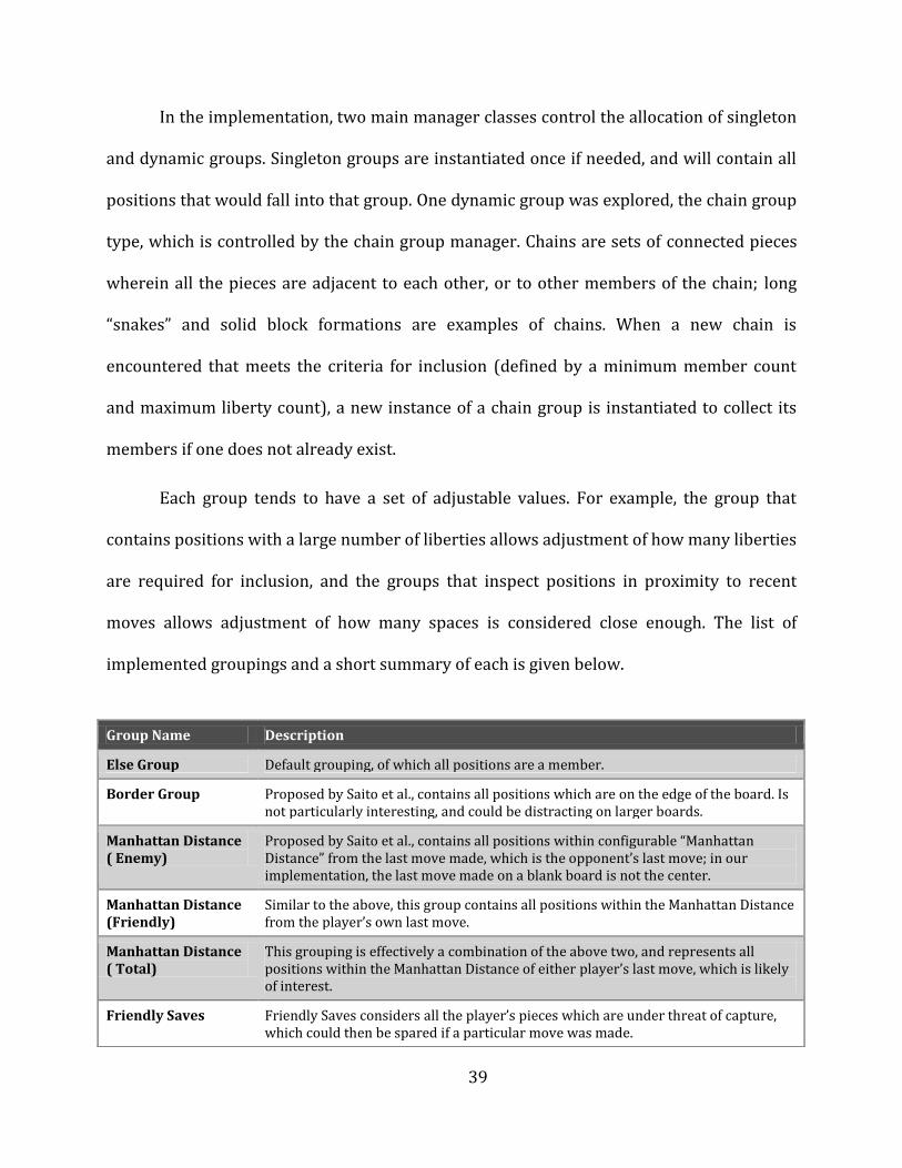
39
In the implementation, two main manager classes control the allocation of singleton
and dynamic groups. Singleton groups are instantiated once if needed, and will contain all
positions that would fall into that group. One dynamic group was explored, the chain group
type, which is controlled by the chain group manager. Chains are sets of connected pieces
wherein all the pieces are adjacent to each other, or to other members of the chain; long
“snakes” and solid block formations are examples of chains. When a new chain is
encountered that meets the criteria for inclusion (defined by a minimum member count
and maximum liberty count), a new instance of a chain group is instantiated to collect its
members if one does not already exist.
Each group tends to have a set of adjustable values. For example, the group that
contains positions with a large number of liberties allows adjustment of how many liberties
are required for inclusion, and the groups that inspect positions in proximity to recent
moves allows adjustment of how many spaces is considered close enough. The list of
implemented groupings and a short summary of each is given below.
Group Name Description
Else Group Default grouping, of which all positions are a member.
Border Group Proposed by Saito et al., contains all positions which are on the edge of the board. Is not particularly interesting, and could be distracting on larger boards.
Manhattan Distance ( Enemy)
Proposed by Saito et al., contains all positions within configurable “Manhattan Distance” from the last move made, which is the opponent’s last move; in our implementation, the last move made on a blank board is not the center.
Manhattan Distance (Friendly)
Similar to the above, this group contains all positions within the Manhattan Distance from the player’s own last move.
Manhattan Distance ( Total)
This grouping is effectively a combination of the above two, and represents all positions within the Manhattan Distance of either player’s last move, which is likely of interest.
Friendly Saves Friendly Saves considers all the player’s pieces which are under threat of capture, which could then be spared if a particular move was made.

40
Table 2.1 – Implemented Groupings
With so many groups implemented, it was necessary to perform preliminary
experiments to eliminate those which performed poorly (did not correlate with winning /
losing moves). Multiple experiments were performed with mixed results. These were taken
into account when designing the final experiment due to the limited availability of
computing resources and time.
2.6 Conclusion
While a significant portion of this project was spent on algorithm design and
development, the main goal was the simulation and analysis of the improvements. During
the entire implementation of UCT-DAG and grouping, preliminary experiments were
conducted. These experiments not only helped to expose problems in the code, but also to
guide our development efforts, especially with respect to the groupings selected for
LibEGO. In addition these experiments provided valuable data that could be used to select
the appropriate simulations to run for the final experiments. This was especially important
Enemy Kills Counterpart of the above, this group spots the opponent’s positions that are under threat of capture and which could be taken with one move.
Enemy Group, Friendly Group, Enemy Threat, Friendly Threat
This set of groups represent pieces placed directly adjacent to enemy/friendly pieces, and positions that are “under threat” and adjacent to that position’s opponent’s piece. They were not intended for practical use on their own.
Many Liberties Positions that would have many liberties (associated free spaces) are in this group.
Chain Group Manager
This group dynamically allocates new chain groups when they are needed. Each set of positions for which a particular chain group is applicable are set into a new chain group.
Chain Group Represents a group that constitutes members of a particular chain. Not intended for practical use by itself.
Friendly Chainmaker
These positions will allow the formation of a chain to occur, possibly by joining together two other smaller chains or single pieces
Enemy Chainmaker These are the positions which would allow the opponent to form a chain.

41
given the finite computing resources and time available for running the experiments. The
specific experiments that were conducted and the data resulting from those experiments
are presented in the next chapter.
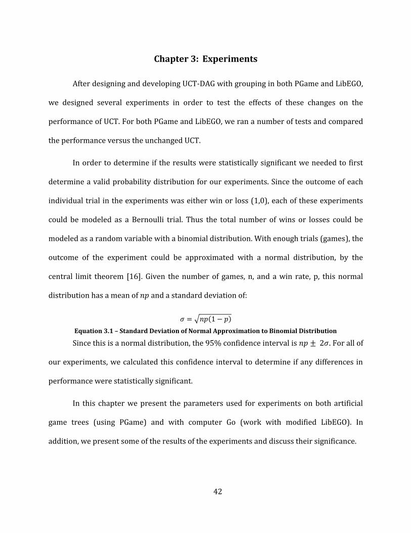
42
Chapter 3: Experiments
After designing and developing UCT-DAG with grouping in both PGame and LibEGO,
we designed several experiments in order to test the effects of these changes on the
performance of UCT. For both PGame and LibEGO, we ran a number of tests and compared
the performance versus the unchanged UCT.
In order to determine if the results were statistically significant we needed to first
determine a valid probability distribution for our experiments. Since the outcome of each
individual trial in the experiments was either win or loss (1,0), each of these experiments
could be modeled as a Bernoulli trial. Thus the total number of wins or losses could be
modeled as a random variable with a binomial distribution. With enough trials (games), the
outcome of the experiment could be approximated with a normal distribution, by the
central limit theorem [16]. Given the number of games, n, and a win rate, p, this normal
distribution has a mean of 𝑛𝑝 and a standard deviation of:
𝜎 = 𝑛𝑝 1 − 𝑝
Equation 3.1 – Standard Deviation of Normal Approximation to Binomial Distribution
Since this is a normal distribution, the 95% confidence interval is 𝑛𝑝 ± 2𝜎. For all of
our experiments, we calculated this confidence interval to determine if any differences in
performance were statistically significant.
In this chapter we present the parameters used for experiments on both artificial
game trees (using PGame) and with computer Go (work with modified LibEGO). In
addition, we present some of the results of the experiments and discuss their significance.

43
3.1 Artificial Game Trees
In order to quantify the effect of the improvements we made to UCT, we designed
two experiments to test the average error versus a number of new parameters that could
be adjusted to observe changes in algorithm behavior. Discussed in the previous chapter,
these parameters included:
DAG Combination Threshold (percentage of nodes to combine together to make a DAG)
UCT Mode (UCT on Tree, UCT-DAG) toggle Number of groups to use Group Bias (relative amount of correlation between groups and either winning or
losing moves) o Ranges from 0 to 1, with 0 indicating that the group should be composed of
0% of the winning moves and 100% of the losing moves, and 1 indicating that the group should be composed of 100% of the winning moves and 0% of the losing moves.
Group Size (relative size of individual groups) Group Overlap (whether or not the group representing ungrouped nodes should
contain all the nodes or just the nodes not in any other group) toggle
In addition there were few parameters available from the original PGame
experiment:
Breadth (the number of children nodes per parent) Depth (the number of levels in the game tree / DAG) Number of Games (the total number of games to perform) Number of Iterations (the number of iterations to run UCT for) Number of Repetitions (the number of times to repeat UCT on the same game)
In the first set of experiments, we focused primarily on testing the effect of the DAG
combination threshold on the performance of the three modes of UCT. These were tested
on several tree sizes. For all of the experiments we ran 200 games each, with 200
repetitions and 10,000 iterations.
44
In the second set of experiments, we focused on the effect of grouping nodes on the
performance of UCT-DAG. We first tested the effect of group bias and group overlap each
using a single, complete group, to form a relative benchmark and confirm the grouping
code was both functional and performed as expected. Next, we tested the effect of the
parameters that controlled the group bias, group size, and the number of groups; for each
of these sets of experiments, the option to allow group overlap was set to true.
For each experiment we generated two plots. First, the average error (or loss rate)
was plotted versus the number of iterations for which each algorithm was run. These plots
are similar to those presented by Levente Kocsis in the original UCT paper and seen in
Figure 1.2 [11]. Next, we plotted the base average error divided by the average error for the
result. This plot shows the relative improvement of each experiment over the base
experiment, and allows an easier comparison between the two different algorithms. Any
changes that were damaging to performance could be just as easily spotted.
One important note with regards to the results in this section is the fact that the
95% confidence interval about the average error, for any given value, generally included
the 0% error case. Thus, in the plots for these experiments we show only the upper half of
the confidence interval. In order to determine if a result is significantly better than a base
result, we look for the upper confidence interval to be less than the mean of the base result.
In essence we examine results for which it can be stated with certain confidence that the
actual mean of the result is less than the sample mean of the base result.
45
The exact parameters used in all of the experiments are available in Appendix A, in
addition, all of the data are available in plots in Appendix C. We present selected plots and
observations in the following two sections.
3.1.1 UCT on Directed Acyclic Graphs
The first set of artificial game tree experiments investigated the effect of the DAG
Combination on the performance of UCT vs. UCT-DAG. We ran experiments using four
different tree breadths and depths, all with approximately one to two million individual
nodes. The DAG Combination threshold was also varied from 0% (equivalent to a tree) to
30% (where 30% of the nodes are combined with other nodes). It is important to note that
this structure is not an arbitrary DAG, but a DAG where all paths to some node are of the
same length. This is most interesting because of its relevance to the game of Go. In Go the
most likely node combinations are results of different move ordering rather than where the
players place the same pieces in the same positions on the board but in a different order. It
is possible to reach the same board position but through a different set of nodes in Go
(primarily through the possibility of node captures), however this is much less likely than
the former.
In the following figure we show the average error for UCT-DAG versus the number
of iterations for all of the DAG combination values on a tree with breadth 2 and depth 20.
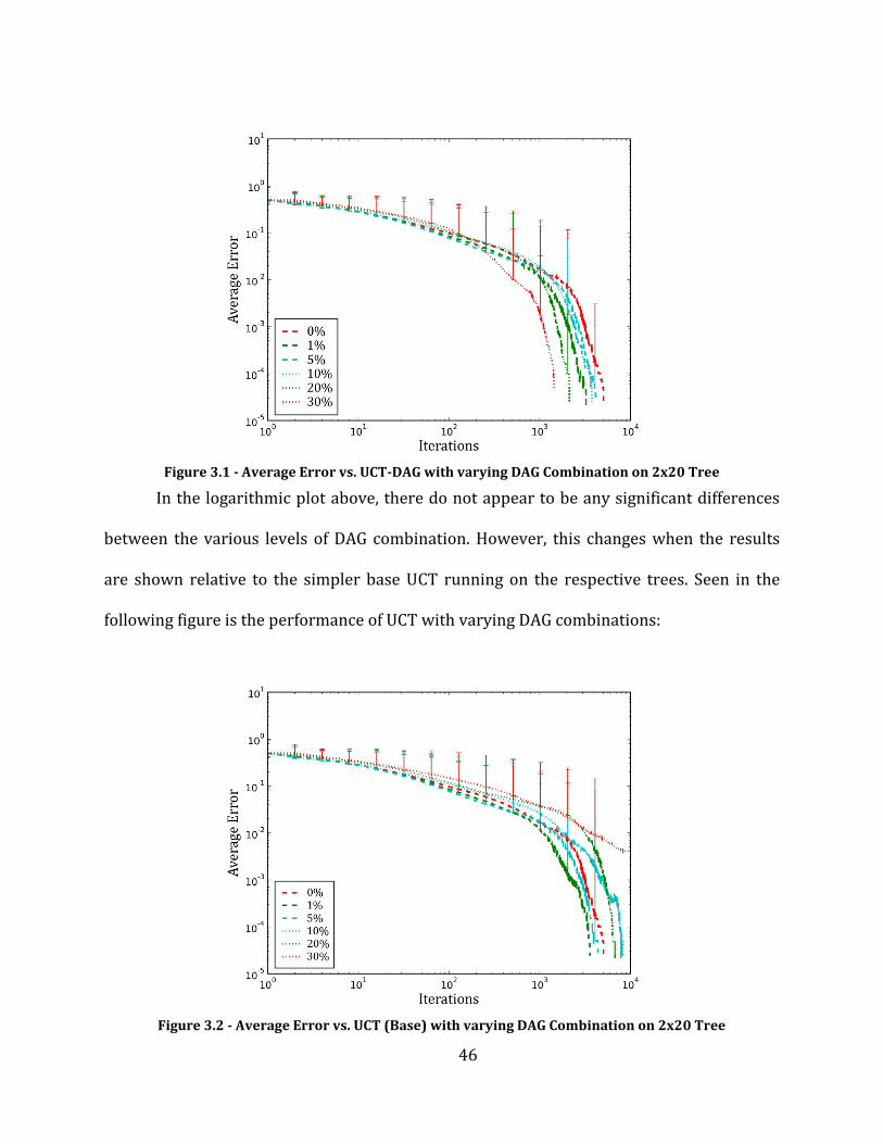
46
Figure 3.1 - Average Error vs. UCT-DAG with varying DAG Combination on 2x20 Tree
In the logarithmic plot above, there do not appear to be any significant differences
between the various levels of DAG combination. However, this changes when the results
are shown relative to the simpler base UCT running on the respective trees. Seen in the
following figure is the performance of UCT with varying DAG combinations:
Figure 3.2 - Average Error vs. UCT (Base) with varying DAG Combination on 2x20 Tree
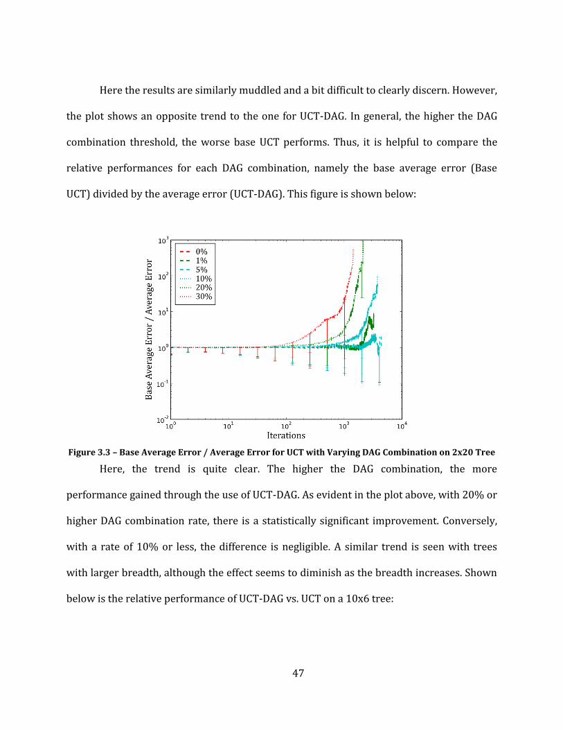
47
Here the results are similarly muddled and a bit difficult to clearly discern. However,
the plot shows an opposite trend to the one for UCT-DAG. In general, the higher the DAG
combination threshold, the worse base UCT performs. Thus, it is helpful to compare the
relative performances for each DAG combination, namely the base average error (Base
UCT) divided by the average error (UCT-DAG). This figure is shown below:
Figure 3.3 – Base Average Error / Average Error for UCT with Varying DAG Combination on 2x20 Tree
Here, the trend is quite clear. The higher the DAG combination, the more
performance gained through the use of UCT-DAG. As evident in the plot above, with 20% or
higher DAG combination rate, there is a statistically significant improvement. Conversely,
with a rate of 10% or less, the difference is negligible. A similar trend is seen with trees
with larger breadth, although the effect seems to diminish as the breadth increases. Shown
below is the relative performance of UCT-DAG vs. UCT on a 10x6 tree:
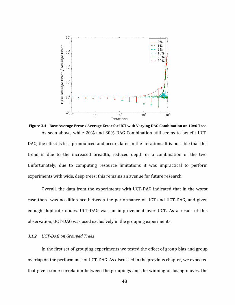
48
Figure 3.4 - Base Average Error / Average Error for UCT with Varying DAG Combination on 10x6 Tree
As seen above, while 20% and 30% DAG Combination still seems to benefit UCT-
DAG, the effect is less pronounced and occurs later in the iterations. It is possible that this
trend is due to the increased breadth, reduced depth or a combination of the two.
Unfortunately, due to computing resource limitations it was impractical to perform
experiments with wide, deep trees; this remains an avenue for future research.
Overall, the data from the experiments with UCT-DAG indicated that in the worst
case there was no difference between the performance of UCT and UCT-DAG, and given
enough duplicate nodes, UCT-DAG was an improvement over UCT. As a result of this
observation, UCT-DAG was used exclusively in the grouping experiments.
3.1.2 UCT-DAG on Grouped Trees
In the first set of grouping experiments we tested the effect of group bias and group
overlap on the performance of UCT-DAG. As discussed in the previous chapter, we expected
that given some correlation between the groupings and the winning or losing moves, the
49
performance of UCT should improve, as it will tend to find the winning moves more
quickly. However, the addition of grouping also increases the size and depth of the DAG, so
each iteration takes longer to complete. To effectively summarize the results of these
experiments we plotted both the average error (fraction of games where UCT chooses the
incorrect move), versus the number of iterations. Similar to the plots in Figure 1.2 [11],
these can help illuminate the relative performance of UCT with the different grouping
parameters.
Initial experiments with grouping showed that on the tree sizes that were practical
to test, group biases less than 0.70 and greater than 0.30 tended to perform the same or
worse than UCT with no grouping. Thus, in the interest of conserving limited
computational resources, we only performed experiments with group biases less than 0.30
and greater than 0.70.
The next two plots show the effect of group bias on UCT performance with no group
overlapping (group overlap disabled). The first shows the results with a tree with a breadth
of 10 and a depth of 6. The group bias for each line is shown in the legend, and the base
UCT running on the tree with no groups is named ‘Base’
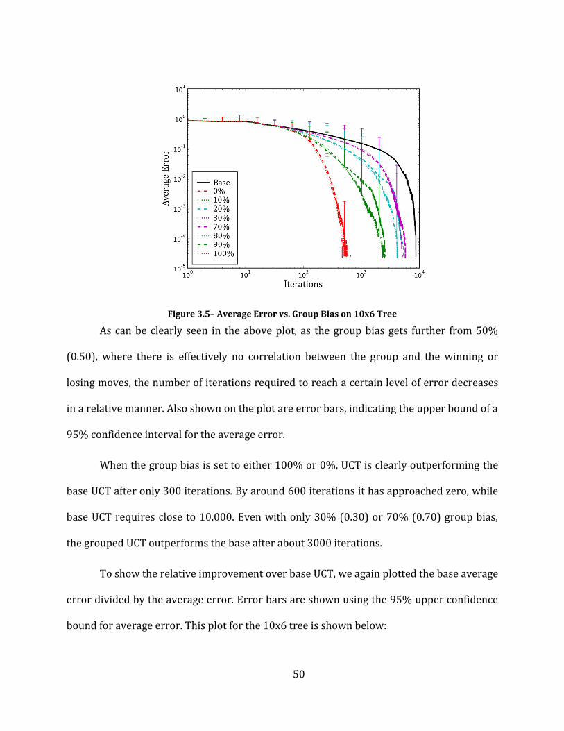
50
Figure 3.5– Average Error vs. Group Bias on 10x6 Tree
As can be clearly seen in the above plot, as the group bias gets further from 50%
(0.50), where there is effectively no correlation between the group and the winning or
losing moves, the number of iterations required to reach a certain level of error decreases
in a relative manner. Also shown on the plot are error bars, indicating the upper bound of a
95% confidence interval for the average error.
When the group bias is set to either 100% or 0%, UCT is clearly outperforming the
base UCT after only 300 iterations. By around 600 iterations it has approached zero, while
base UCT requires close to 10,000. Even with only 30% (0.30) or 70% (0.70) group bias,
the grouped UCT outperforms the base after about 3000 iterations.
To show the relative improvement over base UCT, we again plotted the base average
error divided by the average error. Error bars are shown using the 95% upper confidence
bound for average error. This plot for the 10x6 tree is shown below:
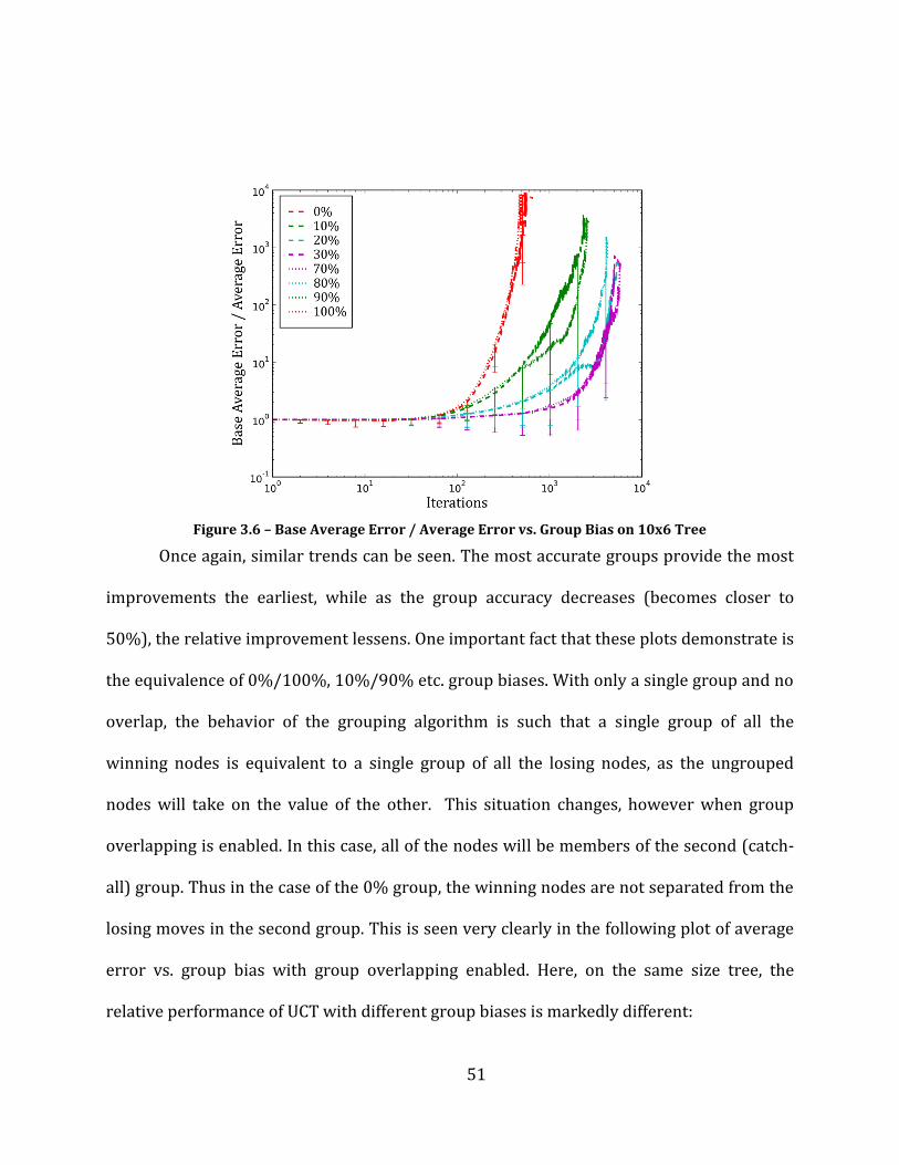
51
Figure 3.6 – Base Average Error / Average Error vs. Group Bias on 10x6 Tree
Once again, similar trends can be seen. The most accurate groups provide the most
improvements the earliest, while as the group accuracy decreases (becomes closer to
50%), the relative improvement lessens. One important fact that these plots demonstrate is
the equivalence of 0%/100%, 10%/90% etc. group biases. With only a single group and no
overlap, the behavior of the grouping algorithm is such that a single group of all the
winning nodes is equivalent to a single group of all the losing nodes, as the ungrouped
nodes will take on the value of the other. This situation changes, however when group
overlapping is enabled. In this case, all of the nodes will be members of the second (catch-
all) group. Thus in the case of the 0% group, the winning nodes are not separated from the
losing moves in the second group. This is seen very clearly in the following plot of average
error vs. group bias with group overlapping enabled. Here, on the same size tree, the
relative performance of UCT with different group biases is markedly different:
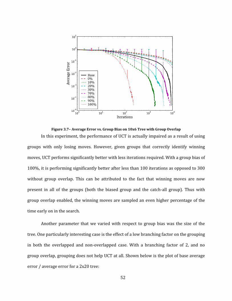
52
Figure 3.7– Average Error vs. Group Bias on 10x6 Tree with Group Overlap
In this experiment, the performance of UCT is actually impaired as a result of using
groups with only losing moves. However, given groups that correctly identify winning
moves, UCT performs significantly better with less iterations required. With a group bias of
100%, it is performing significantly better after less than 100 iterations as opposed to 300
without group overlap. This can be attributed to the fact that winning moves are now
present in all of the groups (both the biased group and the catch-all group). Thus with
group overlap enabled, the winning moves are sampled an even higher percentage of the
time early on in the search.
Another parameter that we varied with respect to group bias was the size of the
tree. One particularly interesting case is the effect of a low branching factor on the grouping
in both the overlapped and non-overlapped case. With a branching factor of 2, and no
group overlap, grouping does not help UCT at all. Shown below is the plot of base average
error / average error for a 2x20 tree:
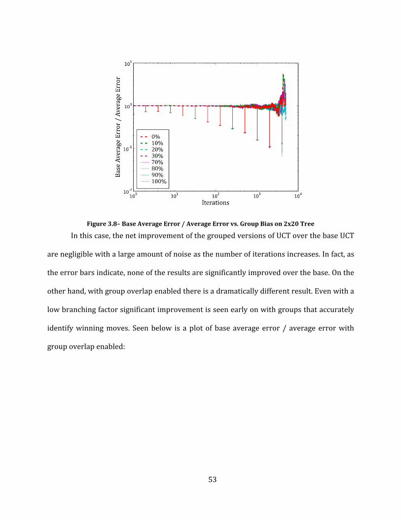
53
Figure 3.8– Base Average Error / Average Error vs. Group Bias on 2x20 Tree
In this case, the net improvement of the grouped versions of UCT over the base UCT
are negligible with a large amount of noise as the number of iterations increases. In fact, as
the error bars indicate, none of the results are significantly improved over the base. On the
other hand, with group overlap enabled there is a dramatically different result. Even with a
low branching factor significant improvement is seen early on with groups that accurately
identify winning moves. Seen below is a plot of base average error / average error with
group overlap enabled:
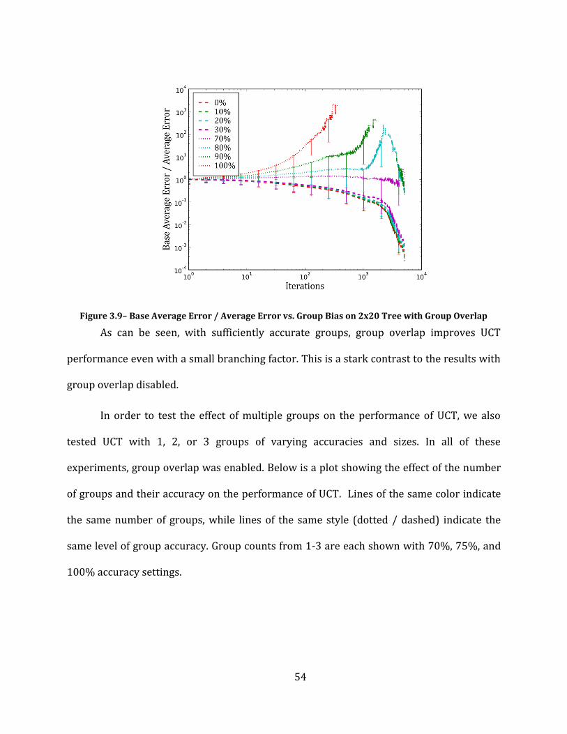
54
Figure 3.9– Base Average Error / Average Error vs. Group Bias on 2x20 Tree with Group Overlap
As can be seen, with sufficiently accurate groups, group overlap improves UCT
performance even with a small branching factor. This is a stark contrast to the results with
group overlap disabled.
In order to test the effect of multiple groups on the performance of UCT, we also
tested UCT with 1, 2, or 3 groups of varying accuracies and sizes. In all of these
experiments, group overlap was enabled. Below is a plot showing the effect of the number
of groups and their accuracy on the performance of UCT. Lines of the same color indicate
the same number of groups, while lines of the same style (dotted / dashed) indicate the
same level of group accuracy. Group counts from 1-3 are each shown with 70%, 75%, and
100% accuracy settings.
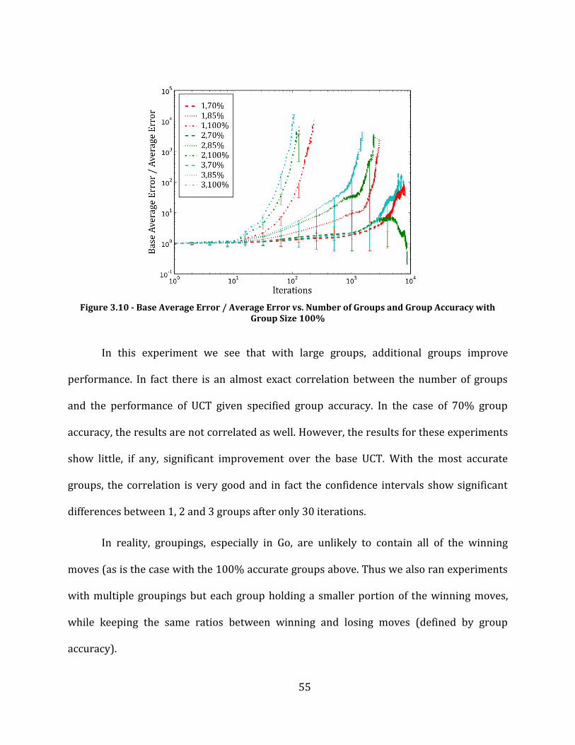
55
Figure 3.10 - Base Average Error / Average Error vs. Number of Groups and Group Accuracy with Group Size 100%
In this experiment we see that with large groups, additional groups improve
performance. In fact there is an almost exact correlation between the number of groups
and the performance of UCT given specified group accuracy. In the case of 70% group
accuracy, the results are not correlated as well. However, the results for these experiments
show little, if any, significant improvement over the base UCT. With the most accurate
groups, the correlation is very good and in fact the confidence intervals show significant
differences between 1, 2 and 3 groups after only 30 iterations.
In reality, groupings, especially in Go, are unlikely to contain all of the winning
moves (as is the case with the 100% accurate groups above. Thus we also ran experiments
with multiple groupings but each group holding a smaller portion of the winning moves,
while keeping the same ratios between winning and losing moves (defined by group
accuracy).
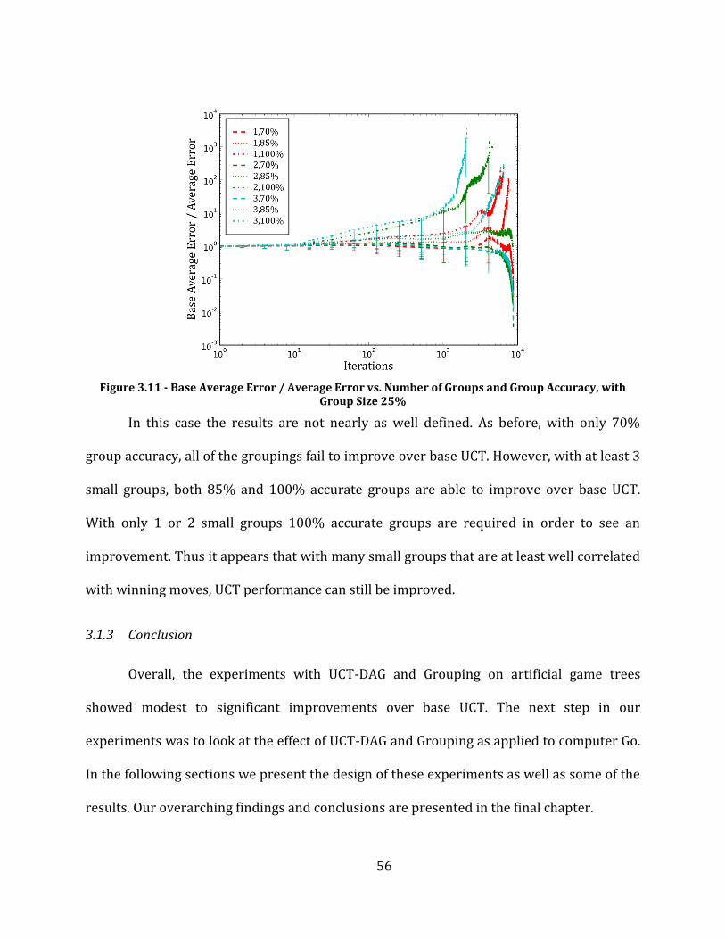
56
Figure 3.11 - Base Average Error / Average Error vs. Number of Groups and Group Accuracy, with Group Size 25%
In this case the results are not nearly as well defined. As before, with only 70%
group accuracy, all of the groupings fail to improve over base UCT. However, with at least 3
small groups, both 85% and 100% accurate groups are able to improve over base UCT.
With only 1 or 2 small groups 100% accurate groups are required in order to see an
improvement. Thus it appears that with many small groups that are at least well correlated
with winning moves, UCT performance can still be improved.
3.1.3 Conclusion
Overall, the experiments with UCT-DAG and Grouping on artificial game trees
showed modest to significant improvements over base UCT. The next step in our
experiments was to look at the effect of UCT-DAG and Grouping as applied to computer Go.
In the following sections we present the design of these experiments as well as some of the
results. Our overarching findings and conclusions are presented in the final chapter.
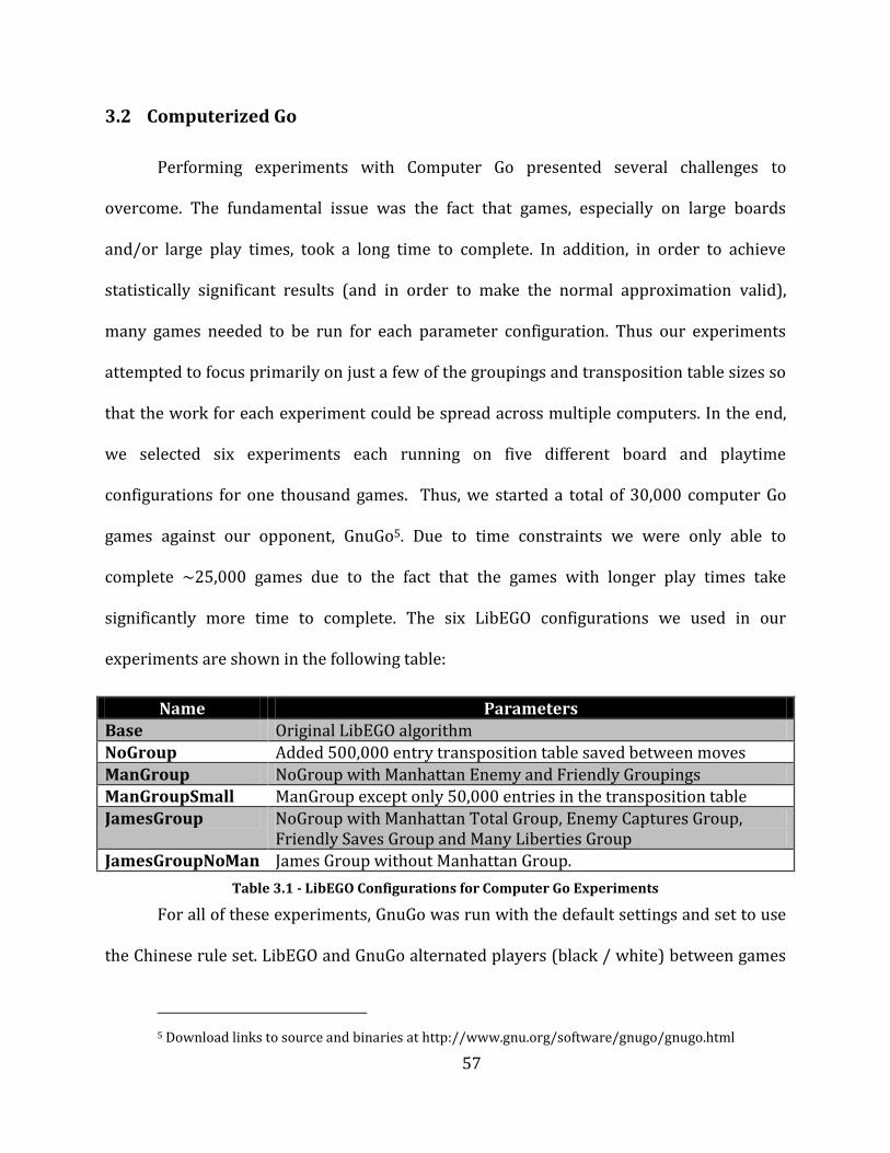
57
3.2 Computerized Go
Performing experiments with Computer Go presented several challenges to
overcome. The fundamental issue was the fact that games, especially on large boards
and/or large play times, took a long time to complete. In addition, in order to achieve
statistically significant results (and in order to make the normal approximation valid),
many games needed to be run for each parameter configuration. Thus our experiments
attempted to focus primarily on just a few of the groupings and transposition table sizes so
that the work for each experiment could be spread across multiple computers. In the end,
we selected six experiments each running on five different board and playtime
configurations for one thousand games. Thus, we started a total of 30,000 computer Go
games against our opponent, GnuGo5. Due to time constraints we were only able to
complete ~25,000 games due to the fact that the games with longer play times take
significantly more time to complete. The six LibEGO configurations we used in our
experiments are shown in the following table:
Name Parameters Base Original LibEGO algorithm
NoGroup Added 500,000 entry transposition table saved between moves
ManGroup NoGroup with Manhattan Enemy and Friendly Groupings ManGroupSmall ManGroup except only 50,000 entries in the transposition table
JamesGroup NoGroup with Manhattan Total Group, Enemy Captures Group, Friendly Saves Group and Many Liberties Group
JamesGroupNoMan James Group without Manhattan Group.
Table 3.1 - LibEGO Configurations for Computer Go Experiments
For all of these experiments, GnuGo was run with the default settings and set to use
the Chinese rule set. LibEGO and GnuGo alternated players (black / white) between games
5 Download links to source and binaries at http://www.gnu.org/software/gnugo/gnugo.html
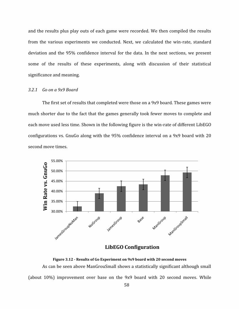
58
and the results plus play outs of each game were recorded. We then compiled the results
from the various experiments we conducted. Next, we calculated the win-rate, standard
deviation and the 95% confidence interval for the data. In the next sections, we present
some of the results of these experiments, along with discussion of their statistical
significance and meaning.
3.2.1 Go on a 9x9 Board
The first set of results that completed were those on a 9x9 board. These games were
much shorter due to the fact that the games generally took fewer moves to complete and
each move used less time. Shown in the following figure is the win-rate of different LibEGO
configurations vs. GnuGo along with the 95% confidence interval on a 9x9 board with 20
second move times.
Figure 3.12 - Results of Go Experiment on 9x9 board with 20 second moves
As can be seen above ManGrouSmall shows a statistically significant although small
(about 10%) improvement over base on the 9x9 board with 20 second moves. While
30.00%
35.00%
40.00%
45.00%
50.00%
55.00%
Win
Ra
te v
s. G
nu
Go
LibEGO Configuration
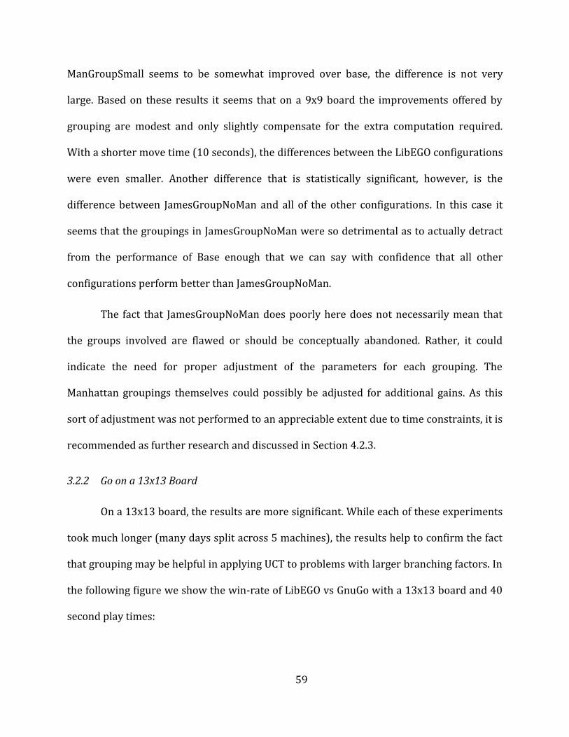
59
ManGroupSmall seems to be somewhat improved over base, the difference is not very
large. Based on these results it seems that on a 9x9 board the improvements offered by
grouping are modest and only slightly compensate for the extra computation required.
With a shorter move time (10 seconds), the differences between the LibEGO configurations
were even smaller. Another difference that is statistically significant, however, is the
difference between JamesGroupNoMan and all of the other configurations. In this case it
seems that the groupings in JamesGroupNoMan were so detrimental as to actually detract
from the performance of Base enough that we can say with confidence that all other
configurations perform better than JamesGroupNoMan.
The fact that JamesGroupNoMan does poorly here does not necessarily mean that
the groups involved are flawed or should be conceptually abandoned. Rather, it could
indicate the need for proper adjustment of the parameters for each grouping. The
Manhattan groupings themselves could possibly be adjusted for additional gains. As this
sort of adjustment was not performed to an appreciable extent due to time constraints, it is
recommended as further research and discussed in Section 4.2.3.
3.2.2 Go on a 13x13 Board
On a 13x13 board, the results are more significant. While each of these experiments
took much longer (many days split across 5 machines), the results help to confirm the fact
that grouping may be helpful in applying UCT to problems with larger branching factors. In
the following figure we show the win-rate of LibEGO vs GnuGo with a 13x13 board and 40
second play times:
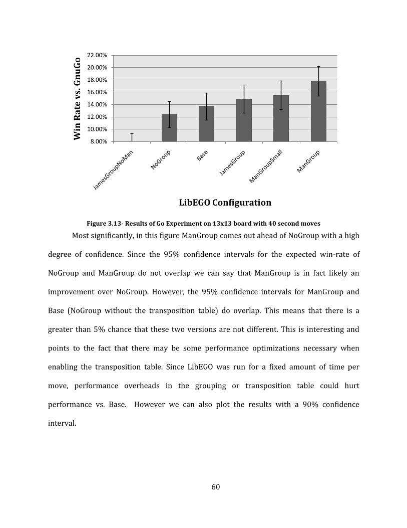
60
Figure 3.13- Results of Go Experiment on 13x13 board with 40 second moves
Most significantly, in this figure ManGroup comes out ahead of NoGroup with a high
degree of confidence. Since the 95% confidence intervals for the expected win-rate of
NoGroup and ManGroup do not overlap we can say that ManGroup is in fact likely an
improvement over NoGroup. However, the 95% confidence intervals for ManGroup and
Base (NoGroup without the transposition table) do overlap. This means that there is a
greater than 5% chance that these two versions are not different. This is interesting and
points to the fact that there may be some performance optimizations necessary when
enabling the transposition table. Since LibEGO was run for a fixed amount of time per
move, performance overheads in the grouping or transposition table could hurt
performance vs. Base. However we can also plot the results with a 90% confidence
interval.
8.00%
10.00%
12.00%
14.00%
16.00%
18.00%
20.00%
22.00%
Win
Ra
te v
s. G
nu
Go
LibEGO Configuration
61
Figure 3.14 – Results of Go Experiment on 13x13 board with 40 second moves (90% confidence intervals)
With 90% confidence intervals shown, ManGroup and Base no longer overlap. Thus
we can say that the probability that ManGroup does not outperform Base is greater than
5% but less than 10%. In addition, it is helpful to note the amount of improvement,
whereas with the 9x9 board, ManGroupSmall showed a 10% improvement over Base, here
we see a 25% improvement. What is also interesting is the role reversal between
ManGroupSmall and ManGroup. In this case the larger transposition table has an advantage
over the small transposition table. While this is not a large enough difference to be
statistically significant, it does show a general reversal of the trend seen on the 9x9 board,
where the small transposition table won out. Once again JamesGroupNoMan performs
badly implying that the groupings used in this configuration do not accurately identify
winning moves.
We also completed experiments with even longer playtimes. However due to the
long times for individual games with these playtimes we were not able to complete enough
8.00%
10.00%
12.00%
14.00%
16.00%
18.00%
20.00%
22.00%
Win
Ra
te v
s. G
nu
Go
LibEGO Configuration
62
games to achieve statistically significant results. However the same general trends were
visible though the differences between Base and ManGroup were smaller. This may imply
that grouping tends to help improve results more early in the search and given more time
Base tends to catch up in terms of accuracy. Plots of these results are shown in Appendix D.
3.2.3 Conclusion
Overall the experiments with computer Go show some interesting trends and some
statistically significant results. Due to the amount of time required for even one game of go,
especially on larger boards, statistically significant results are particularly hard to produce.
However, even with these limitations, we did note some evident improvement through the
use of a large transposition table and the two Manhattan groupings on a 13x13 board. In
the end, however, more experiments would be helpful in order to solidify the current
results and observations.
63
Chapter 4: Conclusion
In this project, the overarching goal was to investigate the performance of UCT as
applied to directed acyclic graphs, as well as to quantify the effect of grouping on UCT
performance. In the following sections we not only summarize our findings with respect to
these two goals, but also present several areas for future research where we saw potential
for additional development and/or experimentation due to the time and computing
constraints of this project.
4.1 Findings
Based on our analysis of the data from experiments performed on both artificial
game trees and computer go simulations, we developed several findings. These findings are
presented in the following sections. For each we refer to the data upon which the finding is
based.
4.1.1 UCT-DAG can improve performance of UCT on complex DAGs and performs equally to UCT on simple DAGs.
In Section 3.1.1, we presented the results of multiple experiments performed
comparing UCT-DAG vs. UCT on DAGs with varying complexity. When looking at the
relative performance of UCT-DAG vs. UCT (see Figure 3.3), with high DAG combination
thresholds (>10%), UCT-DAG showed statistically significant performance games and
generally converged to the correct answer more quickly than plain UCT. In addition, with
lower DAG combination thresholds (0%-10%), UCT-DAG performed equally to UCT. Due to
the simple nature of the UCT-DAG modification (storing node visit counts per parent vs.
64
once per node) as discussed in Section 2.2, performance gains are realized in situations
where DAGs are complex while performance is not harmed in all other cases.
It should be noted, however, that different tree sizes do seem to have an effect on
the relative performance of UCT-DAG; its performance between different board sizes is a
potential area for future experimentation. Regardless, the key fact is that in no case does
UCT-DAG significantly deteriorate performance and thus it is reasonable to implement this
algorithm for any case where a game or simulation representation may be more DAG-like
than tree-like.
4.1.2 Highly correlated, complete groupings dramatically improve performance of UCT on trees with high branching factors.
In Section 3.1.2, we presented the results from experiments with groupings. When
group overlap was disabled (the catch-all group held only nodes that were otherwise
ungrouped), highly correlated groups (either containing mostly winning or losing nodes),
that were complete (held most of the either winning or losing nodes) resulted in
dramatically improved performance over base UCT given a sufficient branching factor (>2).
It is especially important to note the importance of completeness in this result. For
example, given groupings that were completely correlated (either all losing moves or all
winning moves), the grouping bias of 0% or 100% produce essentially equivalent tree
structure. In the case of 0% bias, the group will contain all of the losing moves and due to
the non-overlapped nature of the catch-all group, it will contain all of the winning moves. In
the case of 100% bias, the roles of the group and catch-all group are reversed. If these
groups were not complete (contained less than 100% of the winning or losing moves), this
would not be the case and we would not see such similar results as shown in Figure 3.6.

65
Due to these caveats, this case is in fact not particularly applicable to real world
situations like Go. In Go it is not possible to calculate if any move during all points in the
game is a winning move or a losing move (or else there would be no reason to bother with
a random algorithm to attempt to determine this). So while this finding is interesting, it is
not directly applicable to computer Go as it stands.
4.1.3 Highly accurate, complete groupings with group overlap dramatically improve performance of UCT on any tree.
Our next experiments with grouping involved the effect of enabling group overlap
(where the catch-all group now contains all of the possible nodes, rather than just those
that are not in another group). In this case—as discussed previously—group accuracy
becomes important, with low accuracy (low group bias) reducing performance and high
accuracy (high group bias) increasing performance.
What is perhaps even more interesting is the behavior that arises with group
overlap enabled: highly accurate groups perform even better than before. In addition,
performance is even significantly improved on trees with low branching factors (see Figure
3.9). With group overlap enabled, there are even more paths to the grouped nodes (not
only through the group but also through the catch-all group). Thus, grouped nodes are
explored even more in the beginning of the UCT process. However, once again this
experiment was performed using complete groups and similar to the previous finding is
therefore not directly applicable to the game of Go.
4.1.4 Multiple less-accurate groups, with group overlap, perform similarly to a single more-accurate group.
Our final experiments with grouping tested the effect of group size and the number
of groups on UCT-DAG performance. As seen in Figure 3.11, multiple less-accurate groups
66
can actually perform similarly to a single more accurate group. When groups are
incomplete, and/or less accurate, multiple groupings can actually improve performance.
This result is actually the most promising with regards to computer Go. In this case, any
heuristic groupings that are developed will likely only be somewhat accurate and represent
a small subset of the total number of winning moves available at any point. However, since
it seems that combining several less-accurate groups together can achieve the same
performance gains as a single more-accurate group6, performance gains can still be seen in
computer Go even with smaller, less-accurate groupings (as long as there are a sufficient
number of them).
4.1.5 Accurate groupings in conjunction with UCT-DAG improve the performance of LibEGO vs GnuGo on larger boards.
As discussed in Sections 3.2.1 and 3.2.2, with small boards, grouping, while it
seemed to show some performance gains, the differences between the original UCT and
grouped UCT statistically significant but not very large (10%). On the other hand, with a
13x13 board and a large enough transposition table (500,000 entries), the Manhattan
grouping showed significant improvements over base UCT with a 25% improvement. This
result correlates nicely with the results on artificial game trees, as discussed in Section
3.1.2, where with trees with larger branching factors, accurate groupings improved
performance more quickly and by larger margins on trees with small branching factors.
Thus, grouping (with accurate groups), appears to improve UCT’s performance on larger
6 Intuitively this may not be completely obvious. However, by, for instance, combining 3 groups with
size 0.25 and accuracy 0.70, a total of 0.525 of the winning nodes will be grouped, while 0.225 of the losing nodes will be grouped. On the other hand with a single group of the same size but with accuracy 0.85, only 0.213 of the winning moves will be grouped and 0.038 of the losing moves will be grouped. So while the ratio between winning moves and losing moves in the prior case is worse, the total number of grouped winning nodes in absolute terms is larger.
67
boards and could be used in order to help it to scale up to 19x19 boards. Overall the results
show promise; however, additional experiments with grouping should be performed in
order to gain a better understanding on how groups could be applied. Some possible
avenues for future research in this area are discussed later in this chapter.
4.1.6 The size of the UCT-DAG transposition table may be sensitive to branching factor.
Another trend we saw with our results from the computer Go experiments was that
the transposition table size seems to affect the performance differently given different
board sizes. While the differences were not large enough to be statistically significant, there
was a distinct difference between ManGroup and ManGroupSmall on a 9x9 board which
was reversed on a 13x13 board. This result suggests that the optimal transposition table
size may be different depending on the size of the board. Unfortunately, due to time
limitations, we did not have the opportunity to run additional experiments in order to
verify this result. While it is not certain that transposition table size has an effect on the
performance given different board sizes, this preliminary result warrants further
investigation.
4.2 Future Research
Over the course of our project there were several related areas of research that
became apparent but were outside of the scope of the project due to time or computational
constraints. Ranging from the further improvement of UCT-DAG, to applications of Machine
Learning to Grouping and use of the GRID, there are many interesting opportunities for
further research. While not intending to be an exhaustive list, some possible avenues for
68
future research that were not necessarily mentioned elsewhere in the paper are explored
in the following sections.
4.2.1 UCT-DAG with Multi-Path Update
One major avenue for future research is further updates to UCT-DAG in order to
provide more complete, multi-path updates for each Monte-Carlo simulation. As discussed
in Section 2.2, the current version of UCT-DAG only updates the nodes along the path which
was explored. Since there can be multiple paths to any node in a DAG, it is possible that
UCT accuracy could be improved by updating all the nodes on any path to the node.
However, it is still not clear exactly how this can be accomplished while maintaining the
existing behavior of UCT. In addition, the performance impacts of such multi-path updates
must be taken into account as significant computation could be required in order to
perform such updates. We have provided a general framework for such multi-path updates
with an initial simple implementation. However this implementation does not preserve the
convergence behavior of UCT. By performing further research in this area it is possible that
additional significant gains could be made to further improve UCT’s performance on DAGs.
4.2.2 Transposition Table
Another line of experimentation that was looked into, although not to great enough
an extent to be statistically significant, are the advantages that could be gained by saving
some transposition table data between games, not just between moves. It would be similar
to the use of an opening position library, but it could be computed strictly through the
application itself. However, it would not necessarily show the “right” move to make; just
give more information about the possible moves. Although it would not provide a list of the
69
best moves to make, by integrating the values that were already calculated for certain
moves it would result in a more accurate analysis of the current board position.
In this way, the algorithm is more likely to select a correct move based on the extra-
reliable data. As with storing transposition table data between moves, some effective and
thoughtful algorithm would be desired to prune the table and select which moves should
be kept and for what portion of the game; for example, you would not necessarily want the
transposition table to only store the last 10 moves of a game, which might be relatively
uninteresting territory-filling behavior as is currently expressed by our modified LibEGO.
4.2.3 Online or Offline Determination of Group Biases & Parameter Tuning
In the course of our experimentation, we observed that some groups behaved well
in conjunction with each other (for example, the so-called James Group and its array of
active groupings) but actually caused less accuracy when used alone. While the Manhattan
groupings were able to show success both individually and paired with other groupings, it
appears that most of the other groupings by themselves are contributing rarely enough on
their own that they serve as nothing more than a distraction and create an unnecessary
overhead. We conjectured that this could be compensated for if the amount of
consideration for groups could be biased somehow.
The first idea to test this would involve simply making “dummy” groups that
automatically succeed in grouping, to observe how a group behaves when it is in with a set
of meaningless groups. Taking the idea further and avoiding the extra clutter, we added a
biasing factor to our already-modified LibEGO implementation in order to have greater
control over the group biasing. There was insufficient time to conduct meaningful
experimentation using this group biasing, but it inspired us to consider the implications of
70
online learning of the proper group biases. Given enough time and relatively
straightforward modifications, it would be possible to have the modified UCT-DAG
algorithm learn how useful groups are over time, and thus adjust this biasing factor. For
example, the border group is often not interesting at the start of each game, as these are
typically undesirable moves to make and should be “ignored” early on.
By adjusting this biasing factor on the fly, it would be easy to allow the program to
adjust to changing circumstances and would minimize the amount of pre-calculated data is
required at the start. Additionally, should it be of interest to use biases calculated
beforehand, the online determination of group biases could be used over several games to
determine a suitable bias for each group in an automatable way, rather than checking
various grouping biases by hand. With a suitable bias applied to it, groups that perform
poorly when implemented singly (or in small counts of active groups) could potentially see
improvement and no longer lower the accuracy of UCT-DAG.
Every group was made with a variety of adjustable parameters, controlling factors
such as the range to search around the last moves, or the length of a chain to be potentially
built or harassed by the player. Due to the time constraints, these parameters were not
fully evaluated to determine the optimal tuned value. Only minimal hand adjustment was
possible, and statistically significant experimentation with each adjustment was not
possible due to limited computational resources which were dedicated to testing the core
experiments.
Because of this, it is possible that additional performance gains can be achieved
through the use of online learning and genetic algorithms to slowly hone in on optimal
71
values for these variables. Future research could include determining the best possible
starting values for these parameters, as well as perhaps modifying the main algorithm to
adjust them in real time, similar to how the transposition table will begin implementing
harsher pruning over time. For example, at some point in the game, or for larger boards in
general, it may be beneficial to adjust the Manhattan distance control to allow a larger
region to enter the group. On a larger board, the thresholds for creating and attacking
chains might be interesting to change up, although board size here is partially accounted
for in the current implementation. The overall development and evaluation of entirely new
groupings, with experimental/automated assistance, may also be a desirable topic to
research. The current groupings were made without extensive knowledge of the mechanics
of Go and could benefit from further evaluation.
4.2.4 Using the GRID as a mechanism for Machine Learning with UCT / Grouping
One limitation present throughout our experimentation was the number of
computers we could run tests on. A number of experiments took far too long to easily
repeat enough times to receive data we could be sufficiently confident about. These
limitations meant that we were unable to adequately test larger board sizes, and
conducting tests with 19x19 boards is definitely something that should be done in the
future, to measure the impact of the UCT-DAG modifications and grouping over base UCT
algorithms. According to experiments we performed UCT-DAG shows great gains when the
branching factor is large, which should manifest itself on a 19x19 board.
The GRID at SZTAKI could be put to use as a test bed for experiments, if LibEGO was
given the necessary modifications and properly submitted. The amount of concurrent
experiments that could be run would be much higher, although there is the potential issue
72
of waiting in the queue for access to the computational cluster. The extra processing power
would make research into machine learning much more feasible, especially considering
that a lot of repetition would be required for some of it. If LibEGO was properly parallelized
(the changes required are beyond the scope of this paper), more Monte-Carlo simulations
could be completed in less time as well, yielding more accurate results in a timelier fashion.
4.2.5 UCT/Monte-Carlo Simulation Split: LibEGO & PGame
In LibEGO, Monte Carlo simulations are handled separately from the UCT game tree
itself, as discussed in section 2.1.2; this is due to the large size of a Go play tree and number
of simulations. PGame, on the other hand, maintain the two together (section 2.1.1). It
would be interesting to implement the separation that LibEGO does with the PGame, and
conduct experimentation in that context. LibEGO has a concept of a “maturity level” for
node expansion that requires a certain number of simulations to be performed on any node
before it is expanded for exploration and further consideration.
Modification of this maturity level was not included in the main research performed;
however, it may warrant investigation. Determining which nodes to expand and when
could have a large performance and accuracy impact, and adjust the overall size of the
representative data structure (tree/graph). Additional investigation of maturity levels in
the realm of artificial game trees would also be practical, serving to model the effects of the
changes and provide a more controlled environment for experimentation.
4.3 Summary
While chess has been solved, to the point that computers can consistently win
versus the best human opponents, and is no longer an interesting field of study, being able
73
to defeat humans at Go is a new goal for search algorithm development. The immense
branching factor and nature of the game make it inherently suited to analysis by human
players, and act as obstacles to computerized opponents. A promising new tree-search
algorithm, UCT, promises to give computers the advantage they need; but there are many
aspects of UCT that could be improved.
LibEGO, a basic open-source implementation of UCT that separates its Monte-Carlo
simulation from its tree, is a good starting point for development. We were able to modify
UCT into a new algorithm, UCT-DAG, that managed the Go game as a directed acyclic graph.
This data type is far more suitable in terms of a practical representation of Go, but also had
the potential for performance gains. Storing information that may be useful in the future,
instead of discarding it, also was a new feature that could help boost accuracy and
minimize wasted processor time. By experimenting with grouping behavior and
investigating promising group formation rules, we found methods to optimize how UCT-
DAG would select its moves by allowing it to generalize about sets.
By modifying Levente Kocsis’ PGame program (designed to work on artificial game
trees) to instead have a similar adaptation to directed acyclic graphs, we were able to
validate the modifications to UCT by showing that they worked in a general case—not just
in terms of Go. Experimentations with adjusting game tree breadth/depth and group
membership confirmed the kinds of improvements that we hoped to develop for Go. The
PGame experiments served as an ideal model for the LibEGO modifications in a generalized
form and supported the theoretical aspect of the changes we implemented in UCT: the DAG
was a successful representation of what was once a tree, the groupings worked and showed
74
the potential to improve accurate move selection, and only through very inaccurate and
distracting groupings would performance ever be questionable.
Our practical computerized-Go matches between the modified LibEGO and GnuGo
opponent confirmed what the PGame experiments suggested. The UCT-DAG was able to
boost performance, and generally speaking as a worst-case “only” performed equivalently
to base UCT. In many cases, the modified version was able to converge to the right answer
far sooner than base UCT, which was the best algorithm prior to UCT-DAG and is presently
used in champion computer-Go programs. Transposition tables showed great promise by
allowing data to be saved between moves, or potentially even games. The extra information
that is no longer discarded can be used to form more accurate move selection. Groupings,
while some are weak alone, stand to boost performance greatly, especially on larger
boards. We confirmed that the groupings used need not be complicated theoretically or
practically, or even particularly accurate at spotting favorable moves, and yet they still can
show performance boosts. These relatively straightforward modifications could be
implemented in the UCT-based computer Go champions to give them a boost.
However, there is a need for further investigation as computational resources did
not allow for all the experimentation we would have liked to do. UCT-DAG, bolstered with a
multi-path update, and further work with the transposition table being saved between
games could stand to produce more accurate results, but were not tested much. Modifying
the groupings to properly use online (or offline) learning to bias selection and
consideration is another functionality that, while the groundwork to support it was coded,
was not thoroughly investigated. Research into how LibEGO and PGame respectively split
and do not split the Monte Carlo simulation from the main game is another topic that could
75
be looked into. And while the UCT algorithm could lend itself to use on multi-processor
machines, it would need some work to properly work on a cluster such as the GRID,
allowing for desirable parallelization of operation. Once explored, these areas of research
could combine with the existing modifications to allow computerized Go to pose a
challenge to human players on larger boards, where previously failure was the norm except
on the smallest standard size.
In summary, through this project we developed and tested two major improvements
for UCT. These improvements (UCT-DAG and grouping) represent both original work in the
area of random search algorithms, and extensions of previous work in the area. They
venture to help extend the success of UCT (through Mogo) beyond 9x9 Go boards. Through
experiments on both artificial game trees and with computer go we showed statistically
significant improvements in performance using both UCT-DAG and grouping. In addition
we have identified several areas of future research which, combined with our work will
help to achieve the goal of competitive computer Go on large boards.
76
References
[1] Artificial Intelligence, Winning Ways. The Economist. January 25, 2007.
[2] Auer, Peter, Cesa-Bianchi, Nicolo and Fischer, Paul. Finite-time Analysis of the Multiarmed Bandit Problem. 2002, Machine Learning, pp. 235–256.
[3] Brown, David C. CS 4341 Artificial Intelligence. CS4341 Artificial Intelligence Course Contents. [Online] December 7, 2007. [Cited: April 7, 2008.] http://web.cs.wpi.edu/~dcb/courses/CS4341/2007/contents.html.
[4] Coquelin, Pierre-Arnaud and Munos, Rémi. Bandit Algorithms for Tree Search. 2007, Technical Report INRIA, RR-6141.
[5] Enzenberger, Markus. The Integration of A Priori Knowledge into a Go Playing Neural Network. s.l. : LMU Munich, 1996.
[6] Fotland, David. North American Computer Go Championships. Smart-Games.com. [Online] November 15, 1998. [Cited: April 9, 2008.] http://www.smart-games.com/uscompgo.html.
[7] Gelly, Sylvain. Sylvain GELLY's Home Page. Sylvain GELLY's Home Page. [Online] 2007. [Cited: April 1, 2008.] http://www.lri.fr/~gelly/MoGo.htm.
[8] Gelly, Sylvain, et al. MoGo: Improvements in Monte-Carlo Computer-Go Using UCT and Sequence-Like Simulations. Alberta : s.n., December 12, 2006.
[9] Gergely, Andras. Algorithm helps computers beat human Go players. Reuters. February 21, 2007.
[10] INRIA. MoGo, Master of Go. INRIA Centre de Recherche. [Online] The National Institute for Research in Computer Science and Control, April 9, 2008. [Cited: April 10, 2008.] http://www.inria.fr/saclay/news/mogo-master-of-go.
[11] Kocsis, Levente and Szepesvari, Csaba. Bandit based Monte-Carlo Planning. 2006, European Conference on Machine Learning, pp. 282-293.
[12] McClain, Dylan Loeb. Once Again, Machine Beats Human Champion at Chess. The New York Times. [Online] December 5, 2006. [Cited: March 28, 2008.] http://www.nytimes.com/2006/12/05/crosswords/chess/05cnd-chess.html.
77
[13] Mecholsky, Dr. John J. Monte Carlo Simulations - Class 11C Presentation. Dr. John J. Mecholsky, Jr. [Online] February 11, 2008. [Cited: March 19, 2008.] http://mecholsky.mse.ufl.edu/EMA4714/EMA4714%20S08/Monte_Carlo_ppt.ppt.
[14] Saito, Jahn-Takeshi, et al. Grouping Nodes for Monte-Carlo Tree Search. Maastricht : MICC, Universiteit Maastricht, 2007, Proceedings of the Computer Games Workshop 2007 (CGW 2007)2007), volume 07-06 of MICC Technical Report Series, pp. 125-132.
[15] Taylor, Nathan. Parallelized UCT for Monte Carlo Game-Tree Search. University of Alberta. [Online] January 29, 2008. [Cited: March 28, 2008.] http://ugweb.cs.ualberta.ca/~ntaylor/299as1.pdf.
[16] Tucker, Howard G. An introduction to probability and mathematical statistics. New York : Academic Press, 1962.
[17] Winston, Patrick. Artificial Intelligence, 2nd. Edition. s.l. : Addison-Wesley, 1984.
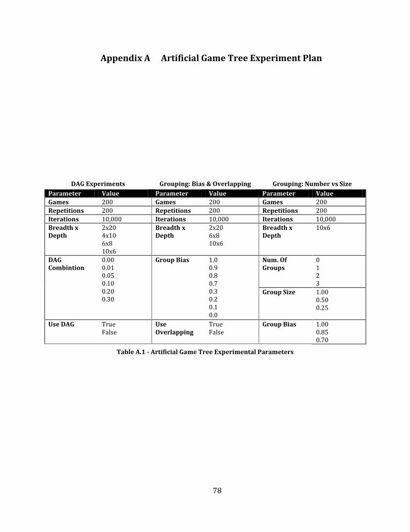
78
Appendix A Artificial Game Tree Experiment Plan
DAG Experiments Grouping: Bias & Overlapping Grouping: Number vs Size
Parameter Value Parameter Value Parameter Value
Games 200 Games 200 Games 200
Repetitions 200 Repetitions 200 Repetitions 200
Iterations 10,000 Iterations 10,000 Iterations 10,000
Breadth x Depth
2x20 4x10 6x8 10x6
Breadth x Depth
2x20 6x8 10x6
Breadth x Depth
10x6
DAG Combintion
0.00 0.01 0.05 0.10 0.20 0.30
Group Bias 1.0 0.9 0.8 0.7 0.3 0.2 0.1 0.0
Num. Of Groups
0 1 2 3
Group Size 1.00 0.50 0.25
Use DAG True False
Use Overlapping
True False
Group Bias 1.00 0.85 0.70
Table A.1 - Artificial Game Tree Experimental Parameters
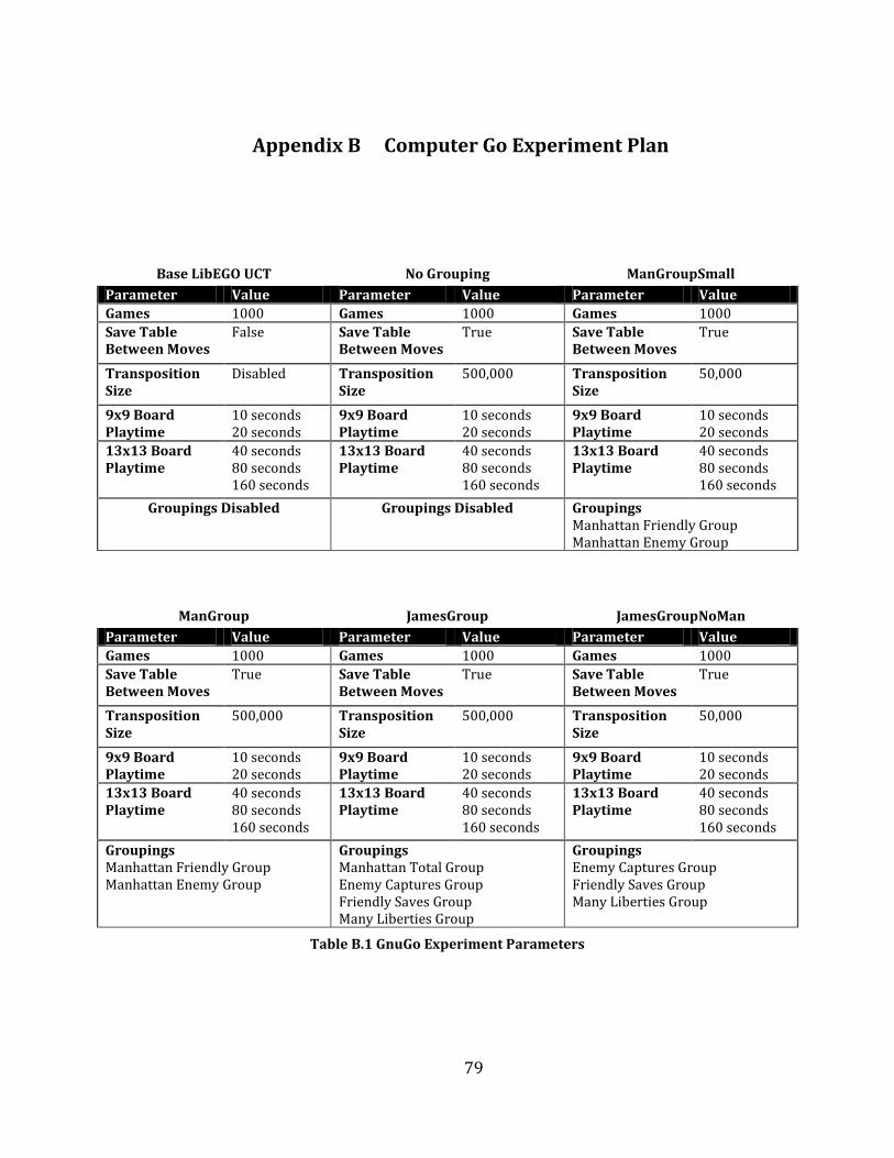
79
Appendix B Computer Go Experiment Plan
Base LibEGO UCT No Grouping ManGroupSmall
Parameter Value Parameter Value Parameter Value
Games 1000 Games 1000 Games 1000
Save Table Between Moves
False Save Table Between Moves
True Save Table Between Moves
True
Transposition Size
Disabled Transposition Size
500,000 Transposition Size
50,000
9x9 Board Playtime
10 seconds 20 seconds
9x9 Board Playtime
10 seconds 20 seconds
9x9 Board Playtime
10 seconds 20 seconds
13x13 Board Playtime
40 seconds 80 seconds 160 seconds
13x13 Board Playtime
40 seconds 80 seconds 160 seconds
13x13 Board Playtime
40 seconds 80 seconds 160 seconds
Groupings Disabled Groupings Disabled Groupings Manhattan Friendly Group Manhattan Enemy Group
ManGroup JamesGroup JamesGroupNoMan
Parameter Value Parameter Value Parameter Value
Games 1000 Games 1000 Games 1000
Save Table Between Moves
True Save Table Between Moves
True Save Table Between Moves
True
Transposition Size
500,000 Transposition Size
500,000 Transposition Size
50,000
9x9 Board Playtime
10 seconds 20 seconds
9x9 Board Playtime
10 seconds 20 seconds
9x9 Board Playtime
10 seconds 20 seconds
13x13 Board Playtime
40 seconds 80 seconds 160 seconds
13x13 Board Playtime
40 seconds 80 seconds 160 seconds
13x13 Board Playtime
40 seconds 80 seconds 160 seconds
Groupings Manhattan Friendly Group Manhattan Enemy Group
Groupings Manhattan Total Group Enemy Captures Group Friendly Saves Group Many Liberties Group
Groupings Enemy Captures Group Friendly Saves Group Many Liberties Group
Table B.1 GnuGo Experiment Parameters
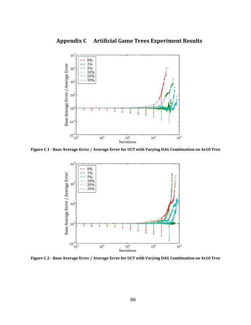
80
Appendix C Artificial Game Trees Experiment Results
Figure C.1 - Base Average Error / Average Error for UCT with Varying DAG Combination on 4x10 Tree
Figure C.2 - Base Average Error / Average Error for UCT with Varying DAG Combination on 4x10 Tree
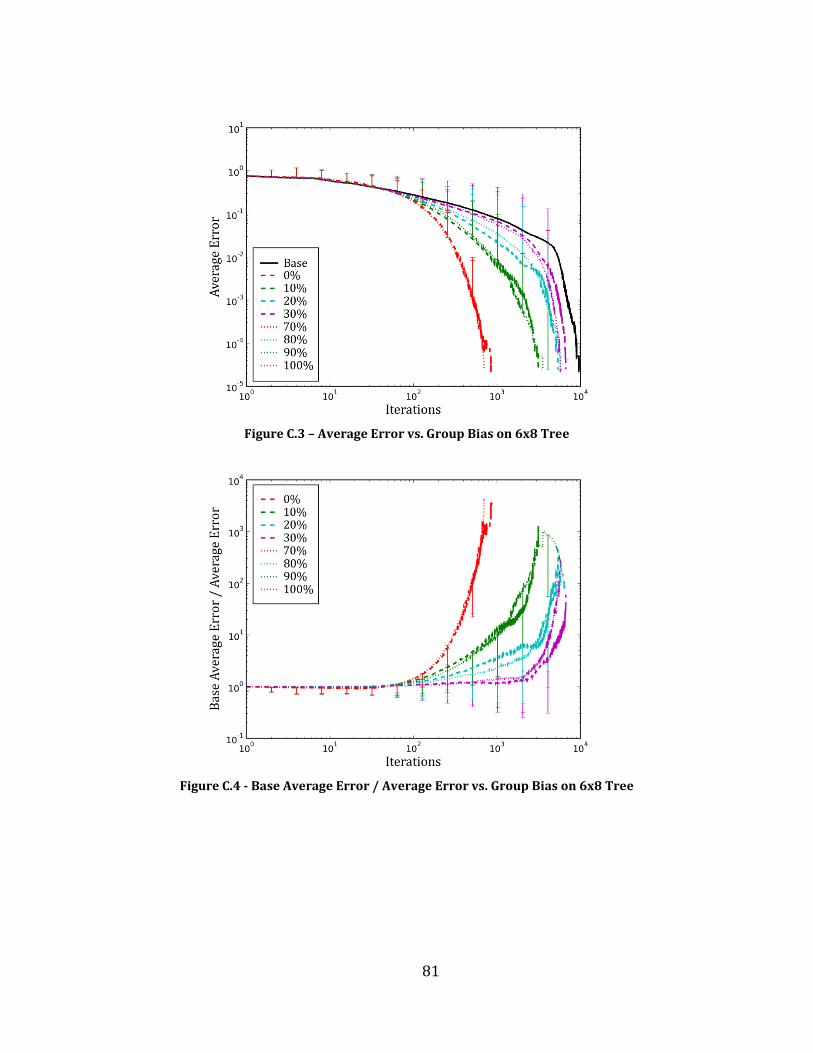
81
Figure C.3 – Average Error vs. Group Bias on 6x8 Tree
Figure C.4 - Base Average Error / Average Error vs. Group Bias on 6x8 Tree
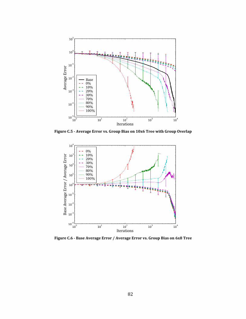
82
Figure C.5 - Average Error vs. Group Bias on 10x6 Tree with Group Overlap
Figure C.6 - Base Average Error / Average Error vs. Group Bias on 6x8 Tree
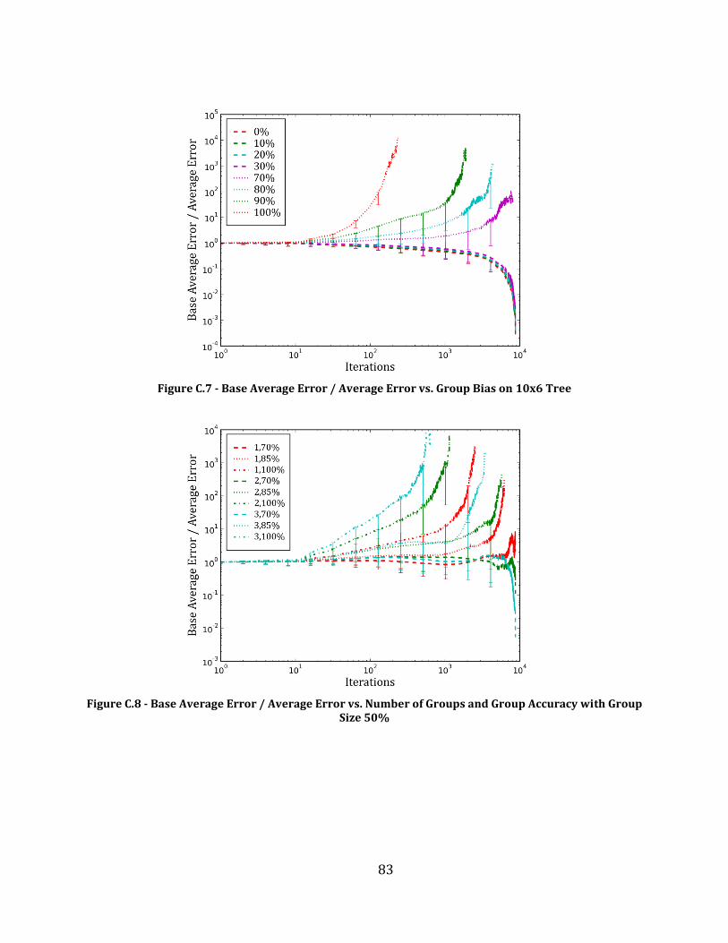
83
Figure C.7 - Base Average Error / Average Error vs. Group Bias on 10x6 Tree
Figure C.8 - Base Average Error / Average Error vs. Number of Groups and Group Accuracy with Group Size 50%
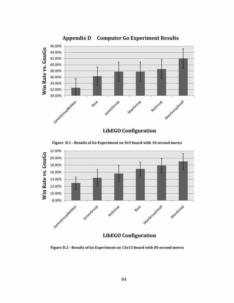
84
Appendix D Computer Go Experiment Results
Figure D.1 - Results of Go Experiment on 9x9 board with 10 second moves
Figure D.2 - Results of Go Experiment on 13x13 board with 80 second moves
30.00%
32.00%
34.00%
36.00%
38.00%
40.00%
42.00%
44.00%
46.00%W
in R
ate
vs.
Gn
uG
o
LibEGO Configuration
8.00%
10.00%
12.00%
14.00%
16.00%
18.00%
20.00%
22.00%
Win
Ra
te v
s. G
nu
Go
LibEGO Configuration
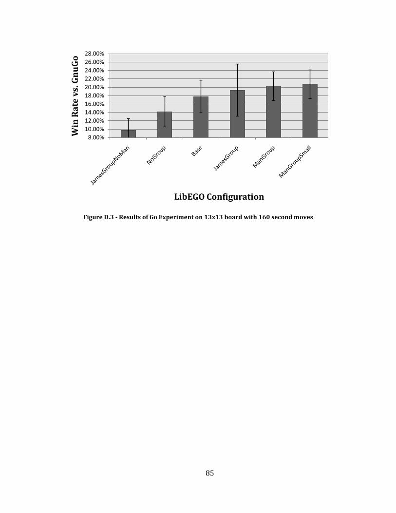
85
Figure D.3 - Results of Go Experiment on 13x13 board with 160 second moves
8.00%
10.00%
12.00%
14.00%
16.00%
18.00%
20.00%
22.00%
24.00%
26.00%
28.00%
Win
Ra
te v
s. G
nu
Go
LibEGO Configuration
86
Appendix E Developer Comments
The source code for the modified version of LibEGO is available on our read-only SVN server at http://svn.bchilds.com/mqp/trunk/ and the source code for the modified PGame program (known as ggame) is available at http://svn.bchilds.com/mqp/branches/ggame/.
To compile LibEGO for general use, rely on the makefile or compile the Visual Studio project for Release. Compiling it for Test will result in a series of grouping tests to be run, on pre-generated test boards (along with audio output if compiling for Win32).
When LibEGO is run, it will execute the automagic.gtp file, which will run a benchmark function on 100,000 Monte-Carlo plays. On an Intel Core2Duo T7300 at 2.00ghz, we averaged about 40kpps (kilo-plays per second). The file can be deleted to skip this step, and benchmarking can be manually run by using the command benchmark <number> to set the number of plays. genmove b and genmove w are used to compute a black and white move, respectively. Type quit to exit the program.
The graphs generated for this project were made using Matplotlib/Pylab, an excellent two-dimensional plotting library using Python. It is available at http://matplotlib.sourceforge.net/ and we highly recommend it for data graphing; it is far easier to use and customize than other graphing tools (such as those that come with Excel), with many output options.
To visualize games, load/save board states, and generate screenshots, as well as acting as a graphical user interface for watching computer vs. computer games, we used GoGui. GoGui supports the GTP (go text protocol) and is available at http://gogui.sourceforge.net/. Our computer opponent was GnuGo 3.6 for Windows, available at http://www.gnu.org/software/gnugo/gnugo.html. A tougher opponent, MoGo release 3 for Windows, is also available at http://www.lri.fr/~gelly/MoGo_Download.htm. To preserve the testing state of each program that was used for our Windows based experimentation, compiled and configured versions of each of these are available on our SVN server at http://svn.bchilds.com/mqp/trunk/gogui/.
To use GoGui, execute the Java archive gogui.jar; gogui-twogtp.jar contains the adapter for allowing two Go programs to compete using GoGui. The command “verbose” will enable all cerr (standard error) output from Go programs to be visible in the GoGui shell display window. Any output you wish to see, such as tree structure drawing, should therefore be output to cerr; output to cout (standard out) will be seen by twogtp as Go commands.
To add a twogtp-moderated competition, in GoGui select Program, New Program, configure twogtp’s command line, set the working directory to wherever the Go programs reside, and then once ready select the option to Attach Program. Select the one you set up. Under Game, be sure to set the proper board size, and set the proper board size for each program you want to use in its command line! Then, set the Computer Player (also under Game) to “both.” To halt the action, set Computer Player to “none” and it will suspend the computer play after the current move is computed.
87
An example twogtp command line setup, that we used during testing, is:
java -jar gogui-twogtp.jar -verbose -black "../Release/libego.exe 10" -white "gnugo-mingw-36.exe --mode gtp" -size 9
This will run LibEGO as the black player with 10 seconds per move, GnuGo as the white player, and set the board dimensions to 9x9. You must set GoGui to use a 9x9 board as well. Select Tools, then GTP Shell (or press F9) to display program text output. Our modified LibEGO, in verbose mode, will display results from its tree and its odds of winning per move; a positive value indicates black is winning, negative indicates white is winning (regardless of LibEGO’s color).