Embed Size (px)
Citation preview

RANDOM NUMBER GENERATION USING CHAOTIC DYNAMICAL MAPS
by
Ali Rıza Ozoren
B.S., Mathematics, Bogazici University, 2007
Submitted to the Institute for Graduate Studies in
Science and Engineering in partial fulfillment of
the requirements for the degree of
Master of Science
Graduate Program in Industrial Engineering
Bogazici University
2011


iii
To my family Yasar, Inci, Murat Ugur and Ozlem Ozoren

iv
ACKNOWLEDGEMENTS
I would like to thank to Yaman Barlas for taking care of almost everything that I
had to overcome during my studies. Besides his guidance and wisdom, his perspective
on Dynamical Systems has changed my point of view on my life. His speed on ana-
lyzing a situation, his genius on detecting the problem on a situation, and his clever
suggestions to solve the problem are really exciting and inspiring for me. I am so
grateful and lucky to have a chance for studying with him.
I want to thank to Wolfgang Hormann and Yagmur Denizhan for participating
in my thesis committee. Their specializations and guidance improved the thesis.
I am very thankful to Serhat Kecici for his true friendship and helps. He, from
my graduate year and on, helped me to adapt the department of industrial engineering
and engineering education after my mathematics education. His point of view as an
engineer is reference for me.
I also thank to Ilker Evrim Colak, who is from my undergraduate year and on.
He has supported me to adapt myself to engineering education since I started the
engineering education. At the earliest times of the thesis, we shared so much time to
study, to discuss, and to laugh together.
And my family: my parents Yasar Ozoren, Inci Ozoren, my brother Murat
Ugur Ozoren and his wife Ozlem Ozoren. I would not be me, or accomplish what I
accomplished so far, if I was not so lucky to have such a family. I am very thankful to
them for raising me, supporting me, and pushing me when I needed a push. They are
an endless support and motivation for me.
I finally thank to Finansbank and my manager Burcu Kula for hiring me without
any difficulties about my graduate education and supporting to complete my graduate
education. I also tahnk to my colleagues in Retail Banking Analytics for their support.

v
ABSTRACT
RANDOM NUMBER GENERATION USING CHAOTIC
DYNAMICAL MAPS
Random numbers are necessary basic ingredients for simulation and modeling.
Currently, linear congruential generators (LCGs) are typically used as random number
generators (RNGs), which generate pseudorandom numbers (PRNs) by using linear
functions and modulus. In this study, we propose some chaotic functions to generate
PRNs, using the unpredictability property of dynamical chaotic maps. We suggest
five different RNGs that are derived from three different chaotic maps: tent map,
logistic map, and family of connecting maps. The uniformity and independence of the
numbers generated through the five suggested RNGs are checked in three steps. Firstly,
the histograms and serial plots are visually checked. Secondly, chi-square and
Kolmogorov-Smirnov tests are applied to statistically test the uniformity of the
generated numbers. Finally, runs tests and autocorrelation test are applied in
order to check the independence of the numbers. The same tests are applied to
compare the five suggested chaotic generators with some well-known conventionally
used LCGs. It is concluded that the suggested generators perform nearly as well as
LCGs and can lead to an alternative way of generating random numbers. More detailed
mathematical, statistical, and numerical properties of the suggested generators
constitute useful further research topics.

vi
OZET
KAOS OZELLIGI OLAN FONKSIYONLARLA RASTGELE
SAYI URETMEK
Rastgele sayılar, simulasyon ve modellemede kullanılan en gerekli
unsurlardandır. Rastgele sayıları uretmek icin en guncel ve yaygın yontem dogrusal
eslesiksel ureteclerdir. Bu uretecler, dogrusal bir fonksiyon ve mod alma islemini
kullanarak sayıları uretir. Bu calısmada ise, kaotik ozelligi olan fonksiyonları
kullanarak rastgele sayılar uretilebilmesi arastırılmaktadır. Kaotik ozellikteki
fonksiyonların tahmin edilemezlik ozelligine dayandırılarak; cadır fonksiyonu,
lojistik fonksiyonu ve birlestirme fonksiyonundan uretilmis bes farklı rastgele sayı ureteci
onerilmektedir. Bu ureteclerin urettigi sayıların, [0, 1] aralıgında duzgun dagıldıgı
ve bagımsız sayılar urettigi uc asamada test edilmistir. Oncelikle, uretilen sayıların
histogramları ve dizisel grafikleri gorsel olarak incelenmistir. Ikinci olarak, uretilen
sayıların istatistiksel olarak duzgun dagıldıkları Ki-kare testi ve Kolmogorov-Smirnov
testi kullanılarak test edilmistir. Son olarak, “Run” testi ve otokorelasyon testi ile
uretilen sayıların bagımsızlıgı test edilmistir. Ayrıca bu testler; onerilen bes uretecin,
cok iyi bilinen ve sıklıkla kullanılan dogrusal eslesiksel ureteclerle kıyaslanırken de
kullanılmıstır. Sonuc olarak, onerilen rastgele sayı ureteclerinin gorsel ve istatistiksel
testlerde dogrusal eslesiksel uretecler kadar basarılı oldukları ve bu ureteclerin rastgele
sayı uretmek icin kullanılabilecekleri ortaya cıkmıstır. Onerilen bu ureteclerin; daha
detaylı matematiksel, istatistiksel ve islemsel ozelliklerinin arastırılması ve incelenmesi
gelecekte yapılacak yararlı arastırma konuları olusturmaktadır.

vii
TABLE OF CONTENTS
ACKNOWLEDGEMENTS . . . . . . . . . . . . . . . . . . . . . . . . . . . . . iv
ABSTRACT . . . . . . . . . . . . . . . . . . . . . . . . . . . . . . . . . . . . . v
OZET . . . . . . . . . . . . . . . . . . . . . . . . . . . . . . . . . . . . . . . . . vi
LIST OF FIGURES . . . . . . . . . . . . . . . . . . . . . . . . . . . . . . . . . ix
LIST OF TABLES . . . . . . . . . . . . . . . . . . . . . . . . . . . . . . . . . . xx
1. INTRODUCTION . . . . . . . . . . . . . . . . . . . . . . . . . . . . . . . . 1
2. CHAOTIC DYNAMICAL MAPS . . . . . . . . . . . . . . . . . . . . . . . . 3
2.1. Shift Map . . . . . . . . . . . . . . . . . . . . . . . . . . . . . . . . . . 8
2.2. Tent Map . . . . . . . . . . . . . . . . . . . . . . . . . . . . . . . . . . 11
2.3. Logistic Map . . . . . . . . . . . . . . . . . . . . . . . . . . . . . . . . 15
2.4. Connecting Maps . . . . . . . . . . . . . . . . . . . . . . . . . . . . . . 16
3. ANALYSIS OF CHAOTIC MAPS AS RNGs . . . . . . . . . . . . . . . . . . 20
3.1. Tent Map (µ = 2) . . . . . . . . . . . . . . . . . . . . . . . . . . . . . . 23
3.2. Tent Map (µ = 2.00005) . . . . . . . . . . . . . . . . . . . . . . . . . . 28
3.3. Logistic Map (ν = 4) . . . . . . . . . . . . . . . . . . . . . . . . . . . . 32
3.4. Connecting Family of Maps (α = 0.999 and α = 1.01) . . . . . . . . . . 38
3.5. Lyapunov Exponents Of The Suggested Maps . . . . . . . . . . . . . . 44
4. COMPARISON BETWEEN FIVE SUGGESTED CHAOTIC MAPS AND
SOME WELL-KNOWN LINEAR CONGRUENTIAL GENERATORS . . . 49
4.1. Linear Congruential Generators (LCGs) . . . . . . . . . . . . . . . . . 49
4.2. Basic Comparison of Five Suggested Chaotic Maps and LCGs . . . . . 60
4.3. Further Analysis and Comparisons of the Suggested Chaotic Maps . . . 64
5. CONCLUSION . . . . . . . . . . . . . . . . . . . . . . . . . . . . . . . . . . 68
APPENDIX A: HISTOGRAMS FOR TENT MAP (µ = 2) . . . . . . . . . . . 70
APPENDIX B: HISTOGRAMS FOR TENT MAP (µ = 2.00005) . . . . . . . 76
APPENDIX C: HISTOGRAMS FOR T-LOGISTIC MAP (ν = 4) . . . . . . . 82
APPENDIX D: HISTOGRAMS FOR CONNECTING MAP (α = 0.999) . . . 88
APPENDIX E: HISTOGRAMS FOR CONNECTING MAP (α = 1.01) . . . . 95
APPENDIX F: HISTOGRAMS FOR LCGs . . . . . . . . . . . . . . . . . . . 102

viii
APPENDIX G: HISTOGRAMS FOR FIVE SUGGESTED MAPS . . . . . . . 106
APPENDIX H: THE STATISTICAL TEST RESULTS - 1 . . . . . . . . . . . 110
APPENDIX I: THE STATISTICAL TEST RESULTS - 2 . . . . . . . . . . . 115
APPENDIX J: THE STATISTICAL TEST RESULTS - 3 . . . . . . . . . . . 120
APPENDIX K: THE STATISTICAL TEST RESULTS - 4 . . . . . . . . . . . 125
APPENDIX L: HISTOGRAMS WITH DIFFERENT SUBINTERVALS . . . 130
REFERENCES . . . . . . . . . . . . . . . . . . . . . . . . . . . . . . . . . . . . 134

ix
LIST OF FIGURES
Figure 2.1. The orbit of the seed x = 0.3 under logistic map (ν = 4). . . . . . 4
Figure 2.2. The orbit of the seeds x = 0.3 and x = 0.31 under logistic map
(ν = 4) are represented by asterix and squares respectively. . . . . 4
Figure 2.3. An example for a one-hump map. . . . . . . . . . . . . . . . . . . 5
Figure 2.4. An example for an 8-hump map. . . . . . . . . . . . . . . . . . . . 6
Figure 2.5. An example for wiggly iterates. . . . . . . . . . . . . . . . . . . . 6
Figure 2.6. The graph of tent map. . . . . . . . . . . . . . . . . . . . . . . . . 11
Figure 2.7. 6th iteration of tent map (µ = 2). . . . . . . . . . . . . . . . . . . 12
Figure 2.8. 4th iteration of connecting map (α = 0.999). . . . . . . . . . . . . 17
Figure 2.9. 4th iteration of connecting map (α = 1.01). . . . . . . . . . . . . 18
Figure 3.1. Tent map (µ = 2): Seed = 0.010666884564, Iteration no = 1000. . 26
Figure 3.2. Tent map (µ = 2): Seed = 0.010666884564, Iteration no = 10000. 26
Figure 3.3. Tent map (µ = 2): Seed = 0.472433844224, Iteration no = 1000. . 26
Figure 3.4. Tent map (µ = 2): Seed = 0.472433844224, Iteration no = 10000. 27
Figure 3.5. Tent map (µ = 2.00005): Seed = 0.819, Iteration no = 1000. . . . 29

x
Figure 3.6. Tent map (µ = 2.00005): Seed = 0.819, Iteration no = 10000. . . . 29
Figure 3.7. Tent map (µ = 2.00005): Seed = 0.07, Iteration no = 1000. . . . . 30
Figure 3.8. Tent map (µ = 2.00005): Seed = 0.07, Iteration no = 10000. . . . 30
Figure 3.9. Histogram for logistic map. . . . . . . . . . . . . . . . . . . . . . . 33
Figure 3.10. The graph of invariant density of logistic map . . . . . . . . . . . 34
Figure 3.11. Histogram for transformed logistic map (T-logistic map). . . . . . 34
Figure 3.12. T-logistic map (ν = 4): Seed = 0.774, Iteration no = 1000. . . . . 35
Figure 3.13. T-logistic map (ν = 4): Seed = 0.774, Iteration no = 10000. . . . 35
Figure 3.14. T-logistic map (ν = 4): Seed = 0.174, Iteration no = 1000. . . . . 36
Figure 3.15. T-logistic map (ν = 4): Seed = 0.174, Iteration no = 10000. . . . 36
Figure 3.16. The graph of connecting maps (α = 0.999 and α = 1.01). . . . . . 38
Figure 3.17. Connecting map (α = 0.999): Seed = 0.727, Iteration no = 1000. . 39
Figure 3.18. Connecting map (α = 0.999): Seed = 0.727, Iteration no = 10000. 39
Figure 3.19. Connecting map (α = 0.999): Seed = 0.819, Iteration no = 1000. . 40
Figure 3.20. Connecting map (α = 0.999): Seed = 0.819, Iteration no = 10000. 40
Figure 3.21. Connecting map (α = 1.01): Seed = 0.0006, Iteration no = 1000. . 40

xi
Figure 3.22. Connecting map (α = 1.01): Seed = 0.0006, Iteration no = 10000. 41
Figure 3.23. Connecting map (α = 1.01): Seed = 0.8066, Iteration no = 1000. . 41
Figure 3.24. Connecting map (α = 1.01): Seed = 0.8066, Iteration no = 10000. 41
Figure 4.1. MLCG 1: Seed = 931, Iteration no = 1000. . . . . . . . . . . . . . 50
Figure 4.2. MLCG 1: Seed = 931, Iteration no = 10000. . . . . . . . . . . . . 51
Figure 4.3. MLCG 1: Seed = 6647, Iteration no = 1000. . . . . . . . . . . . . 51
Figure 4.4. MLCG 1: Seed = 6647, Iteration no = 10000. . . . . . . . . . . . 51
Figure 4.5. MLCG 2: Seed = 13, Iteration no = 1000. . . . . . . . . . . . . . 52
Figure 4.6. MLCG 2: Seed = 13, Iteration no = 10000. . . . . . . . . . . . . . 52
Figure 4.7. MLCG 2: Seed = 36509, Iteration no = 1000. . . . . . . . . . . . 53
Figure 4.8. MLCG 2: Seed = 36509, Iteration no = 10000. . . . . . . . . . . . 53
Figure 4.9. LCG 3: Seed = 1637, Iteration no = 1000. . . . . . . . . . . . . . 54
Figure 4.10. LCG 3: Seed = 1637, Iteration no = 10000. . . . . . . . . . . . . . 54
Figure 4.11. LCG 3: Seed = 5161, Iteration no = 1000. . . . . . . . . . . . . . 54
Figure 4.12. LCG 3: Seed = 5161, Iteration no = 10000. . . . . . . . . . . . . . 55
Figure 4.13. LCG 4: Seed = 42807, Iteration no = 1000. . . . . . . . . . . . . . 56

xii
Figure 4.14. LCG 4: Seed = 42807, Iteration no = 10000. . . . . . . . . . . . . 56
Figure 4.15. LCG 4: Seed = 11, Iteration no = 1000. . . . . . . . . . . . . . . 57
Figure 4.16. LCG 4: Seed = 11, Iteration no = 10000. . . . . . . . . . . . . . . 57
Figure 4.17. LCG 5: Seed = 6625, Iteration no = 1000. . . . . . . . . . . . . . 58
Figure 4.18. LCG 5: Seed = 6625, Iteration no = 10000. . . . . . . . . . . . . . 58
Figure 4.19. LCG 5: Seed = 87, Iteration no = 1000. . . . . . . . . . . . . . . 58
Figure 4.20. LCG 5: Seed = 87, Iteration no = 10000. . . . . . . . . . . . . . . 59
Figure 4.21. The (xn, xn+1) graphs of chaotic maps. . . . . . . . . . . . . . . . 65
Figure 4.22. The (xn, xn+1) graph of LCGs. . . . . . . . . . . . . . . . . . . . . 66
Figure A.1. Tent map (µ = 2): Seed = 0.197600506499, Iteration no = 1000. . 70
Figure A.2. Tent map (µ = 2): Seed = 0.197600506499, Iteration no = 10000. 70
Figure A.3. Tent map (µ = 2): Seed = 0.231069988461, Iteration no = 1000. . 71
Figure A.4. Tent map (µ = 2): Seed = 0.231069988461, Iteration no = 10000. 71
Figure A.5. Tent map (µ = 2): Seed = 0.98388083416, Iteration no = 1000. . . 71
Figure A.6. Tent map (µ = 2): Seed = 0.98388083416, Iteration no = 10000. . 72
Figure A.7. Tent map (µ = 2): Seed = 0.389913876011, Iteration no = 1000. . 72

xiii
Figure A.8. Tent map (µ = 2): Seed = 0.389913876011, Iteration no = 10000. 72
Figure A.9. Tent map (µ = 2): Seed = 0.455019664777, Iteration no = 1000. . 73
Figure A.10. Tent map (µ = 2): Seed = 0.455019664777, Iteration no = 10000. 73
Figure A.11. Tent map (µ = 2): Seed = 0.490444465331, Iteration no = 1000. . 73
Figure A.12. Tent map (µ = 2): Seed = 0.490444465331, Iteration no = 10000. 74
Figure A.13. Tent map (µ = 2): Seed = 0.086948882143, Iteration no = 1000. . 74
Figure A.14. Tent map (µ = 2): Seed = 0.086948882143, Iteration no = 10000. 74
Figure A.15. Tent map (µ = 2): Seed = 0.686808244224, Iteration no = 1000. . 75
Figure A.16. Tent map (µ = 2): Seed = 0.686808244224, Iteration no = 10000. 75
Figure B.1. Tent map (µ = 2.00005): Seed = 0.945195357852, Iteration no =
1000. . . . . . . . . . . . . . . . . . . . . . . . . . . . . . . . . . . 76
Figure B.2. Tent map (µ = 2.00005): Seed = 0.945195357852, Iteration no =
10000. . . . . . . . . . . . . . . . . . . . . . . . . . . . . . . . . . 76
Figure B.3. Tent map (µ = 2.00005): Seed = 0.005382078128663, Iteration no
= 1000. . . . . . . . . . . . . . . . . . . . . . . . . . . . . . . . . . 77
Figure B.4. Tent map (µ = 2.00005): Seed = 0.005382078128663, Iteration no
= 10000. . . . . . . . . . . . . . . . . . . . . . . . . . . . . . . . . 77
Figure B.5. Tent map (µ = 2.00005): Seed = 0.385874582044063, Iteration no
= 1000. . . . . . . . . . . . . . . . . . . . . . . . . . . . . . . . . . 77

xiv
Figure B.6. Tent map (µ = 2.00005): Seed = 0.385874582044063, Iteration no
= 10000. . . . . . . . . . . . . . . . . . . . . . . . . . . . . . . . . 78
Figure B.7. Tent map (µ = 2.00005): Seed = 0.991, Iteration no = 1000. . . . 78
Figure B.8. Tent map (µ = 2.00005): Seed = 0.991, Iteration no = 10000. . . . 78
Figure B.9. Tent map (µ = 2.00005): Seed = 0.517, Iteration no = 1000. . . . 79
Figure B.10. Tent map (µ = 2.00005): Seed = 0.517, Iteration no = 10000. . . . 79
Figure B.11. Tent map (µ = 2.00005): Seed = 0.197600506499, Iteration no =
1000. . . . . . . . . . . . . . . . . . . . . . . . . . . . . . . . . . . 79
Figure B.12. Tent map (µ = 2.00005): Seed = 0.197600506499, Iteration no =
10000. . . . . . . . . . . . . . . . . . . . . . . . . . . . . . . . . . 80
Figure B.13. Tent map (µ = 2.00005): Seed = 0.267781590398, Iteration no =
1000. . . . . . . . . . . . . . . . . . . . . . . . . . . . . . . . . . . 80
Figure B.14. Tent map (µ = 2.00005): Seed = 0.267781590398, Iteration no =
10000. . . . . . . . . . . . . . . . . . . . . . . . . . . . . . . . . . 80
Figure B.15. Tent map (µ = 2.00005): Seed = 0.897496645632, Iteration no =
1000. . . . . . . . . . . . . . . . . . . . . . . . . . . . . . . . . . . 81
Figure B.16. Tent map (µ = 2.00005): Seed = 0.897496645632, Iteration no =
10000. . . . . . . . . . . . . . . . . . . . . . . . . . . . . . . . . . 81
Figure C.1. T-logistic map (ν = 4): Seed = 0.973, Iteration no = 1000. . . . . 82
Figure C.2. T-logistic map (ν = 4): Seed = 0.973, Iteration no = 10000. . . . 82

xv
Figure C.3. T-logistic map (ν = 4): Seed = 0.912091805655299, Iteration no =
1000. . . . . . . . . . . . . . . . . . . . . . . . . . . . . . . . . . . 83
Figure C.4. T-logistic map (ν = 4): Seed = 0.912091805655299, Iteration no =
10000. . . . . . . . . . . . . . . . . . . . . . . . . . . . . . . . . . 83
Figure C.5. T-logistic map (ν = 4): Seed = 0.68, Iteration no = 1000. . . . . . 83
Figure C.6. T-logistic map (ν = 4): Seed = 0.68, Iteration no = 10000. . . . . 84
Figure C.7. T-logistic map (ν = 4): Seed = 0.58, Iteration no = 1000. . . . . . 84
Figure C.8. T-logistic map (ν = 4): Seed = 0.58, Iteration no = 10000. . . . . 84
Figure C.9. T-logistic map (ν = 4): Seed = 0.282, Iteration no = 1000. . . . . 85
Figure C.10. T-logistic map (ν = 4): Seed = 0.282, Iteration no = 10000. . . . 85
Figure C.11. T-logistic map (ν = 4): Seed = 0.4, Iteration no = 1000. . . . . . 85
Figure C.12. T-logistic map (ν = 4): Seed = 0.4, Iteration no = 10000. . . . . . 86
Figure C.13. T-logistic map (ν = 4): Seed = 0.758167338031333, Iteration no =
1000. . . . . . . . . . . . . . . . . . . . . . . . . . . . . . . . . . . 86
Figure C.14. T-logistic map (ν = 4): Seed = 0.758167338031333, Iteration no =
10000. . . . . . . . . . . . . . . . . . . . . . . . . . . . . . . . . . 86
Figure C.15. T-logistic map (ν = 4): Seed = 0.809, Iteration no = 1000. . . . . 87
Figure C.16. T-logistic map (ν = 4): Seed = 0.809, Iteration no = 10000. . . . 87

xvi
Figure D.1. Connecting map (α = 0.999): Seed = 0.1, Iteration no = 1000. . . 88
Figure D.2. Connecting map (α = 0.999): Seed = 0.1, Iteration no = 10000. . 88
Figure D.3. Connecting map (α = 0.999): Seed = 0.98, Iteration no = 1000. . 89
Figure D.4. Connecting map (α = 0.999): Seed = 0.98, Iteration no = 10000. . 89
Figure D.5. Connecting map (α = 0.999): Seed = 0.6811, Iteration no = 1000. 89
Figure D.6. Connecting map (α = 0.999): Seed = 0.6811, Iteration no = 10000. 90
Figure D.7. Connecting map (α = 0.999): Seed = 0.002, Iteration no = 1000. . 90
Figure D.8. Connecting map (α = 0.999): Seed = 0.002, Iteration no = 10000. 90
Figure D.9. Connecting map (α = 0.999): Seed = 0.7, Iteration no = 1000. . . 91
Figure D.10. Connecting map (α = 0.999): Seed = 0.7, Iteration no = 10000. . 91
Figure D.11. Connecting map (α = 0.999): Seed = 0.298698545648568, Iteration
no = 1000. . . . . . . . . . . . . . . . . . . . . . . . . . . . . . . . 92
Figure D.12. Connecting map (α = 0.999): Seed = 0.298698545648568, Iteration
no = 10000. . . . . . . . . . . . . . . . . . . . . . . . . . . . . . . 92
Figure D.13. Connecting map (α = 0.999): Seed = 0.525620161505902, Iteration
no = 1000. . . . . . . . . . . . . . . . . . . . . . . . . . . . . . . . 93
Figure D.14. Connecting map (α = 0.999): Seed = 0.525620161505902, Iteration
no = 10000. . . . . . . . . . . . . . . . . . . . . . . . . . . . . . . 93

xvii
Figure D.15. Connecting map (α = 0.999): Seed = 0.333, Iteration no = 1000. . 94
Figure D.16. Connecting map (α = 0.999): Seed = 0.333, Iteration no = 10000. 94
Figure E.1. Connecting map (α = 1.01): Seed = 0.672551918078352, Iteration
no = 1000. . . . . . . . . . . . . . . . . . . . . . . . . . . . . . . . 95
Figure E.2. Connecting map (α = 1.01): Seed = 0.672551918078352, Iteration
no = 10000. . . . . . . . . . . . . . . . . . . . . . . . . . . . . . . 95
Figure E.3. Connecting map (α = 1.01): Seed = 0.189, Iteration no = 1000. . 96
Figure E.4. Connecting map (α = 1.01): Seed = 0.189, Iteration no = 10000. . 96
Figure E.5. Connecting map (α = 1.01): Seed = 0.747, Iteration no = 1000. . 96
Figure E.6. Connecting map (α = 1.01): Seed = 0.747, Iteration no = 10000. . 97
Figure E.7. Connecting map (α = 1.01): Seed = 0.880223477310122, Iteration
no = 1000. . . . . . . . . . . . . . . . . . . . . . . . . . . . . . . . 97
Figure E.8. Connecting map (α = 1.01): Seed = 0.880223477310122, Iteration
no = 10000. . . . . . . . . . . . . . . . . . . . . . . . . . . . . . . 98
Figure E.9. Connecting map (α = 1.01): Seed = 0.9, Iteration no = 1000. . . . 98
Figure E.10. Connecting map (α = 1.01): Seed = 0.9, Iteration no = 10000. . . 99
Figure E.11. Connecting map (α = 1.01): Seed = 0.361436078541452, Iteration
no = 1000. . . . . . . . . . . . . . . . . . . . . . . . . . . . . . . . 99

xviii
Figure E.12. Connecting map (α = 1.01): Seed = 0.361436078541452, Iteration
no = 10000. . . . . . . . . . . . . . . . . . . . . . . . . . . . . . . 100
Figure E.13. Connecting map (α = 1.01): Seed = 0.6001, Iteration no = 1000. . 100
Figure E.14. Connecting map (α = 1.01): Seed = 0.6001, Iteration no = 10000. 100
Figure E.15. Connecting map (α = 1.01): Seed = 0.24, Iteration no = 1000. . . 101
Figure E.16. Connecting map (α = 1.01): Seed = 0.24, Iteration no = 10000. . 101
Figure F.1. MLCG 1: Seed = 3316779, Iteration no = 1000. . . . . . . . . . . 102
Figure F.2. MLCG 1: Seed = 3316779, Iteration no = 10000. . . . . . . . . . . 102
Figure F.3. MLCG 2: Seed = 3316779, Iteration no = 1000. . . . . . . . . . . 103
Figure F.4. MLCG 2: Seed = 3316779, Iteration no = 10000. . . . . . . . . . . 103
Figure F.5. LCG 3: Seed = 3316779, Iteration no = 1000. . . . . . . . . . . . 103
Figure F.6. LCG 3: Seed = 3316779, Iteration no = 10000. . . . . . . . . . . . 104
Figure F.7. LCG 4: Seed = 3316779, Iteration no = 1000. . . . . . . . . . . . 104
Figure F.8. LCG 4: Seed = 3316779, Iteration no = 10000. . . . . . . . . . . . 104
Figure F.9. LCG 5: Seed = 3316779, Iteration no = 1000. . . . . . . . . . . . 105
Figure F.10. LCG 5: Seed = 3316779, Iteration no = 10000. . . . . . . . . . . . 105
Figure G.1. Tent map (µ = 2): Seed = 0.03316779, Iteration no = 1000. . . . . 106

xix
Figure G.2. Tent map (µ = 2): Seed = 0.033167, Iteration no = 10000. . . . . 106
Figure G.3. Tent map (µ = 2.00005): Seed = 0.3316, Iteration no = 1000. . . . 107
Figure G.4. Tent map (µ = 2.00005): Seed = 0.33167, Iteration no = 10000. . 107
Figure G.5. T-logistic map (ν = 4): Seed = 0.33167, Iteration no = 1000. . . . 107
Figure G.6. T-logistic map (ν = 4): Seed = 0.3316779, Iteration no = 10000. . 108
Figure G.7. Connecting map (α = 0.999): Seed = 0.3316779, Iteration no =
1000. . . . . . . . . . . . . . . . . . . . . . . . . . . . . . . . . . . 108
Figure G.8. Connecting map (α = 0.999): Seed = 0.3316779, Iteration no =
10000. . . . . . . . . . . . . . . . . . . . . . . . . . . . . . . . . . 108
Figure G.9. Connecting map (α = 1.01): Seed = 0.3316, Iteration no = 1000. . 109
Figure G.10. Connecting map (α = 1.01): Seed = 0.3316, Iteration no = 10000. 109
Figure L.1. Histograms for MLCG 1: Seed = 56623185, Iteration no = 10000. 131
Figure L.2. Histograms for LCG 3: Seed = 56623185, Iteration no = 10000. . 132
Figure L.3. Histogram for connecting map (α = 1.01): Seed = 0.56623185,
Iteration no = 10000. . . . . . . . . . . . . . . . . . . . . . . . . . 133

xx
LIST OF TABLES
Table 3.1. The statistical test results for 10 different seeds under tent map
with parameter µ = 2: Iteration no = 1000. . . . . . . . . . . . . . 27
Table 3.2. The statistical test results for 10 different seeds under tent map
(µ = 2): Iteration no = 10000. . . . . . . . . . . . . . . . . . . . . 28
Table 3.3. The statistical test results for 10 different seeds under tent map
(µ = 2.00005): Iteration no = 1000. . . . . . . . . . . . . . . . . . 31
Table 3.4. The statistical test results for 10 different seeds under tent map
(µ = 2.00005): Iteration no = 10000. . . . . . . . . . . . . . . . . . 32
Table 3.5. The statistical test results for 10 different seeds under T-logistic
map (ν = 4): Iteration no = 1000. . . . . . . . . . . . . . . . . . . 37
Table 3.6. The statistical test results for 10 different seeds under T-logistic
map (ν = 4): Iteration no = 10000. . . . . . . . . . . . . . . . . . 38
Table 3.7. The statistical test results for 10 different seeds under connecting
map (α = 0.999): Iteration no = 1000. . . . . . . . . . . . . . . . . 42
Table 3.8. The statistical test results for 10 different seeds under connecting
map (α = 0.999): Iteration no = 10000. . . . . . . . . . . . . . . . 43
Table 3.9. The statistical test results for 10 different seeds under connecting
map (α = 1.01): Iteration no = 1000. . . . . . . . . . . . . . . . . 43
Table 3.10. The statistical test results for 10 different seeds under connecting
map (α = 1.01): Iteration no = 10000. . . . . . . . . . . . . . . . . 44

xxi
Table 3.11. Number of chi-square tests passed with 10 different seeds for two
connecting maps (p-values of 0.05 is used as the test criteria). . . . 46
Table 4.1. List of some well-known linear congruential generators (LCGs). . . 50
Table 4.2. The statistical test results for two different seeds under MLCG 1. . 52
Table 4.3. The statistical test results for two different seeds under MLCG 2. . 53
Table 4.4. The statistical test results for two different seeds under LCG 3. . . 55
Table 4.5. The statistical test results for two different seeds under LCG 4. . . 57
Table 4.6. The statistical test results for two different seeds under LCG 5. . . 59
Table 4.7. The statistical test results for LGCs and five suggested maps: Seed
= 3316779, Iteration no = 1000. . . . . . . . . . . . . . . . . . . . 61
Table 4.8. The statistical test results for LGCs and five suggested maps: Seed
= 3316779, Iteration no = 10000. . . . . . . . . . . . . . . . . . . . 61
Table 4.9. Number of tests passed with 20 different seeds under LGCs and five
suggested maps (p-values of 0.05 is used as the test criteria). . . . 62
Table 4.10. Number of tests passed with 20 different seeds under LGCs and five
suggested maps (p-values of 0.01 is used as the test criteria). . . . 63
Table 4.11. The statistical test results for LCGs and five suggested maps: Seed
= 915612027, Iteration no = 1000. . . . . . . . . . . . . . . . . . . 67
Table H.1. The statistical test results: Seed = 449, Iteration no = 1000. . . . 110

xxii
Table H.2. The statistical test results: Seed = 181081, Iteration no = 1000. . 110
Table H.3. The statistical test results: Seed = 890123, Iteration no = 1000. . 111
Table H.4. The statistical test results: Seed = 1, Iteration no = 1000. . . . . . 111
Table H.5. The statistical test results: Seed = 9301, Iteration no = 1000. . . . 112
Table H.6. The statistical test results: Seed = 56623185, Iteration no = 1000. 112
Table H.7. The statistical test results: Seed = 27683, Iteration no = 1000. . . 113
Table H.8. The statistical test results: Seed = 77, Iteration no = 1000. . . . . 113
Table H.9. The statistical test results: Seed = 74601189, Iteration no = 1000. 114
Table I.1. The statistical test results: Seed = 89, Iteration no = 1000. . . . . 115
Table I.2. The statistical test results: Seed = 590223, Iteration no = 1000. . 115
Table I.3. The statistical test results: Seed = 39818, Iteration no = 1000. . . 116
Table I.4. The statistical test results: Seed = 123, Iteration no = 1000. . . . 116
Table I.5. The statistical test results: Seed = 6979, Iteration no = 1000. . . . 117
Table I.6. The statistical test results: Seed = 821129, Iteration no = 1000. . 117
Table I.7. The statistical test results: Seed = 91561202, Iteration no = 1000. 118
Table I.8. The statistical test results: Seed = 112319, Iteration no = 1000. . 118

xxiii
Table I.9. The statistical test results: Seed = 277, Iteration no = 1000. . . . 119
Table I.10. The statistical test results: Seed = 4612967, Iteration no = 1000. . 119
Table J.1. The statistical test results: Seed = 449, Iteration no = 10000. . . . 120
Table J.2. The statistical test results: Seed = 181081, Iteration no = 10000. . 120
Table J.3. The statistical test results: Seed = 890123, Iteration no = 10000. . 121
Table J.4. The statistical test results: Seed = 1, Iteration no = 10000. . . . . 121
Table J.5. The statistical test results: Seed = 9301, Iteration no = 10000. . . 122
Table J.6. The statistical test results: Seed = 566231, Iteration no = 10000. . 122
Table J.7. The statistical test results: Seed = 27683, Iteration no = 10000. . 123
Table J.8. The statistical test results: Seed = 77, Iteration no = 10000. . . . 123
Table J.9. The statistical test results: Seed = 746011, Iteration no = 10000. . 124
Table K.1. The statistical test results: Seed = 89, Iteration no = 10000. . . . 125
Table K.2. The statistical test results: Seed = 590223, Iteration no = 10000. . 125
Table K.3. The statistical test results: Seed = 39818317, Iteration no = 10000. 126
Table K.4. The statistical test results: Seed = 123, Iteration no = 10000. . . . 126
Table K.5. The statistical test results: Seed = 6979, Iteration no = 10000. . . 127

xxiv
Table K.6. The statistical test results: Seed = 821129, Iteration no = 10000. . 127
Table K.7. The statistical test results: Seed = 915612, Iteration no = 10000. . 128
Table K.8. The statistical test results: Seed = 112319, Iteration no = 10000. . 128
Table K.9. The statistical test results: Seed = 277, Iteration no = 10000. . . . 129
Table K.10. The statistical test results: Seed = 4612967, Iteration no = 10000. 129
Table L.1. The chi-square test results for MLCG 1, LCG 3, and connecting
map (α = 1.01): Seed = 56623185, Iteration no = 10000. . . . . . 130

1
1. INTRODUCTION
A sequence of numbers that are chosen at random is a necessary basic ingredient in
simulation, modeling and analysis in general. There are two types of random numbers:
The true random numbers are completely unpredictable, and irreproducible. This
kind of sequence can only be generated by a physical process, for instance, by electrical
circuits or physical experiments like dice rolling. The pseudorandom numbers (PRNs)
are on the other hand computed by numerical algorithms. They are supposed to appear
random to someone who does not know the algorithm, and also pass the relevant
statistical tests. Therefore these numbers are reproducible by the numerical algorithm,
and they are most commonly used in simulations. In this work, the generation of the
PRNs by constructing algorithms based on chaotic dynamical maps will be studied.
There is an enormous amount of scientific literature on random number
generation. A short historical overview is presented by Law and Kelton [1]. The
introduction to the properties of random numbers and the generation methods of
random number are covered by Banks [2], and they are particularized by Knuth
[3]. The random number generators (RNGs) have to generate nicely distributed ran-
dom numbers. Nicely distributed means that the sequence of the generated random
numbers is uniformly distributed between zero and one, and dense in this interval.
Secondly, random numbers must be serially independent of each other. Good RNGs
have also the following properties: long periodicity, repeatability, long disjoint
sequences, portability, and efficiency [4].
Over the years, various linear PRN generators have been developed. They are
classified into three categories. Linear congruential generator (LCG) and multiplicative
linear congruential generator (MLCG) are famous and the most widely used techniques
for generating random numbers. MLCG, first used by D.H. Lehmer in 1948, has a
period of about approximately 109 on a 32-bit machine. Fibonacci random number
generator and Tausworthe generators are the other two well-known generators that
are based on computation of each number by performing some usual operations being

2
addition, subtraction, and the ‘exclusive-or’ operation on the two preceding numbers.
These generators have a period of about approximately 10170 on a 32-bit machine [4].
Besides such well-known linear PRN generators, three relatively new RNGs
exist: Generalized feedback shift register (GFSR), twisted generalized feedback shift
register (TGFSR), and Mersenne Twister (MT). GFSR is suggested in 1973 by Lewis
and Payne [13]; and statistically analyzed in 1987 by H. Niederreiter [6]. TGFSR,
a modified version of GFSR, is suggested in 1992 by Matsumoto and Kurita [7] and
improved in 1994 by them [8]. These two generators have a period of about 10200 on a
32-bit machine. MT is developed in 1998 by Matsumoto and Nishimura [9]. It has a
very long period of about 106000 on a 32-bit machine.
The main goal of RNG research is to design robust generators without
having to pay too much in terms of portability, flexibility, and efficiency. A good RNG
should possess long period, high speed, and reliability. Moreover, generated random
numbers have to be independent and uniformly distributed between 0 and 1. In
order to check independency and uniformity of them, serial (dependence) tests and
uniformity tests can be performed [2]. If the sequence of generated numbers passes
these tests satisfactorily, it is considered to be random.
In this thesis we will construct PRN generators based on chaotic dynamical maps
and analyze their statistical properties. We have considered tent map, logistic map and
family of connecting maps as potential RNGs. These maps are very simple and they
may generate random numbers faster than well-known linear RNGs. Also they provide
entirely different methods of producing PRNs. There have been earlier attempts to
use the logistic map as a random number generator [5]. But the chaotic maps that we
consider and complete statistical analysis of results have not been previously published
in the literature.

3
2. CHAOTIC DYNAMICAL MAPS
The motion of anything or the change in a situation implies dynamics in general.
The swinging of a clock pendulum, the insulin level of blood, the flow of water in a
pipe, the number of fish each spring time in a lake, and the human population of earth
are basic examples of systems containing dynamics. A dynamical map encodes the law
of change. It is simply defined as a map f : V → V where V represents the set of all
possible states of the map. The sequence (x, f(x), f(f(x)), f(f(f(x))), ...) is the orbit
of dynamical map for the seed x ∈ V . The orbit is called a periodic orbit if there exists
n ∈ N such that x = fn(x), an eventually periodic orbit if there exist n,m ∈ N such
that fm(x) = fn(x), and a dense orbit in V if there exist a point x ∈ V such that the
orbit is dense in V .
Dynamical maps can exhibit chaotic behavior. Sometimes the orbits starting at
two initial states x0 and x1 eventually get far apart no matter how close two states x0
and x1 are. This makes predicting the long term future of the map very difficult if the
initial state x0 is not known exactly. Such maps are called chaotic, (see Figure 2.1). A
chaotic dynamical map is generally characterized by three properties: Being sensitive to
the initial states (butterfly effect), being topologically transitive, and having a dense
collection of points with periodic orbits. These properties can be translated to the
mathematical language. Devaney defines them as follows [14, 15]:
Definition 2.1 Let V be a set. The dynamical map defined by f : V → V is chaotic
on V if
(i) f has sensitive dependence on initial conditions:
There exists δ > 0 such that, for any x ∈ V and any neighborhood X ⊂ V around
x, there exists y ∈ X and n ∈ N such that |fn(x)− fn(y)| > δ. The number δ is
called a sensitivity constant at x for the map f .
(ii) f is topologically transitive:
For any pair of open sets X, Y ⊂ V , there exists k ∈ N such that fk(X)∩Y 6= ∅.

4
(iii) Periodic points of f is dense in V :
For any open subset X of V X ∩ P 6= ∅, where P is the set of periodic points of
f in V .
Figure 2.1: The orbit of the seed x = 0.3 under logistic map (ν = 4).
The first condition of Devaney’s definition is related with the future of the states.
According to the first condition, It is not predictable how much the distance of two
different close states will be after some iterations. For instance, logistic map with
parameter ν = 4 generates unpredictable numbers starting from the closest seeds 0.3,
and 0.31. As seen in Figure 2.2, the numbers generated starting from seeds 0.3 and
0.31 get apart from each other after the 5th iteration. In other words, small change in
the initial states causes huge change in the following states.
Figure 2.2: The orbit of the seeds x = 0.3 and x = 0.31 under logistic map (ν = 4) are
represented by asterix and squares respectively.
The second and third conditions of Devaney’s definition are topological
conditions. Transitivity controls whether any sequence of generated numbers contains

5
an element, which is the element of the arbitrarily small set determined before, or not.
Namely, an arbitrarily small set is first determined in the range of chaotic map, and
then it is controlled that the map generates a number that is the element of the set
determined. The last ingredient related with the denseness of the periodic orbits of
map. It guarantees that a periodic orbit is always in any subset of the range of map.
These subsets can be arbitrarily small sets.
In general, it is hard to check the chaotic behavior of dynamical maps by showing
three properties directly. There are some methods to prove the chaotic behaviour of
dynamical maps. One of the methods is to observe the natural behavior of map. For
instance, having the wiggly iterates of a map is a way to prove the chaotic behavior of
it. Before defining the wiggly iterates, we consider the definition of a one-hump map
(see Figure 2.3), the definition of a m-hump map (see Figure 2.4), and a lemma related
with a one-hump map which are defined by Banks [16].
Definition 2.2 A continuous map f : [a, c] → [0, 1] is a one-hump map if strictly
increases from f(a) = 0 to f(b) = 1, and then strictly decreases to f(c) = 0.
Figure 2.3: An example for a one-hump map.
Definition 2.3 fn is an n-hump map on [0, 1] if there are n+ 1 points,
0 = x0 < x1 < ... < xn = 1,

6
such that fn is a one-hump map on each interval [xi−1, xi]. This interval is called the
base of the ith hump of fn.
Figure 2.4: An example for an 8-hump map.
Lemma 2.1 If f is a one-hump map on [0, 1] then fn is a 2n−1- hump map on [0, 1].
Definition 2.3 and Lemma 2.1 are two ingredients of the definition of wiggly
iterates [16]. A map f has wiggly iterates if fn is a 2n−1- hump map on for each
positive integer n, and the length of the largest base of the humps of fn tends to zero
as n tends to infinity, (see Figure 2.5).
Figure 2.5: An example for wiggly iterates.
If a map f : [0, 1] → [0, 1] has wiggly iterates, then f is chaotic on the interval
[0, 1] [16]. The proof of the statement is easy when the following lemmas and Devaney’s
definition (Definition 2.1) are taken into account.
Lemma 2.2 If f : [0, 1]→ [0, 1] has wiggly iterates, then
7
• f has sensitive dependence everywhere with sensitivity constant 12,
• f is transitive,
• the set of periodic points of f is dense in [0, 1].
The other method is to find a topologically conjugate between a chaotic
dynamical map and an unknown dynamical map. In this method, two dynamical
maps are connected to each other via a homeomorphism. Homeomorphism carries
all properties of one map to other one. By this way, the chaotic behavior of an
unknown dynamical map is ensured with homeomorphism. The definition of
topologically conjugate, and the theorem related with topologically conjugate and chaos
are included in Banks [16].
Definition 2.4 A map f : V → V is topologically conjugate to a map g : W → W if
there is homeomorphism h : V → W such that h ◦ f = g ◦ h.
Theorem 2.1 Let f and g be topologically conjugate via a homeomorphism h. If f is
chaotic, then so is g.
There is also a useful theorem to detect the chaotic behavior of a map. In fact,
the theorem consists of a kind of simple computation [16].
Theorem 2.2 Let f : [0, 1]→ [0, 1] be a three times differentiable and symmetric one-
hump map. If f ′(0) > 1 and if f has a negative Schwarzian derivative except at x = 12
(Schwarzianderivative : S(f)(x) = 2f ′(x)f ′′′(x) − 3(f ′′(x))2 for all x ∈ [0, 1]), then
the restriction of f to its Cantor set 1 has chaotic behavior.
Lastly, we accompany a useful theorem to establish relations with topologically
transitivity of a dynamical map and a dense orbit. This theorem is important since it
1Cantor set is constructed by the iterations of the map f , see [16]
8
connects two ingredients of the definition of chaos: topologically transitivity, and
denseness of periodic points. The proof of lemmas and theorems can be found in
Banks [16].
Theorem 2.3 If V is a compact metric space, then f is topologically transitive if and
only if there exists a point x ∈ V such that {fn(x) : n ∈ N} is dense in V .
The chaotic features of maps: tent map, logistic map, and the family of
connecting maps can be analyzed with the theorems and the lemmas. We will
follow the specified order to show the chaotic behaviour of the maps. It is hard to
show the chaotic behaviour of tent map directly. We will try to find topologically
conjugacy between a chaotic dynamical map, which is shift map, and tent map. Firstly,
we will consider shift map and investigate its chaotic behavior. Then, we will
define tent map and determine topologically conjugate between tent map and itself.
Secondly, we will examine logistic map. The chaotic behaviour of it will be shown by
two ways: determining topologically conjugacy between tent map and logistic map,
and computing Schwarzian derivative to apply Theorem 2.2. Lastly, we will examine
the family of two connecting maps, and investigate their chaotic behaviour by using
Lemma 2.2.
2.1. Shift Map
Let Σ2 be the space of the infinite sequences on an alphabet of two symbols,
denoted by 0 and 1 (i.e. Σ2 = {(s0s1s2...) : sj ∈ {0, 1}}). Define the metric between
two elements s = (s0s1s2...) and t = (t0t1t2...) of Σ2 by:
d (s, t) =∞∑i=0
|si − ti|2i
Now, we can determine the most useful property of the metric d:

9
Proposition 2.1 Let s, t ∈ Σ2 and suppose si = ti for i = 1, 2, ..., n. Then d (s, t) ≤
1/2n. Conversely, if d (s, t) < 1/2n, then si = ti for i ≤ n.
Let s, t ∈ Σ2 and suppose si = ti for i = 1, 2, ..., n. Consider d (s, t):
d (s, t) =∞∑i=0
|si − ti|2i
=∞∑
i=n+1
|si − ti|2i
≤∞∑
i=n+1
1
2i=
1
2n.
Conversely; assume sk 6= tk for some k ≤ n. Then,
d (s, t) =∞∑i=0
|si − ti|2i
=1
2k+
∞∑i=n+1
|si − ti|2i
=1
2k+
1
2n≥ 1
2n.
Definition 2.5 Shift Map σ : Σ2 → Σ2 is defined by
σ(s0s1s2s3...) = (s1s2s3s4...)
where (s0s1s2...) ∈ Σ2.
In other words, when the shift map is applied to a sequence s ∈ Σ2, the first
entry s0 of s is deleted to produce σ(s). The fact that the shift map σ is continuous
and chaotic:
Proposition 2.2 The shift map σ is continuous on Σ2 with respect to metric d.
Let ε > 0 be given and s, t ∈ Σ2. We can find n ∈ N such that 12n< ε. Take
δ = 12n+1 such that d (s, t) < δ. By Proposition 2.1, si = ti for i ≤ n + 1, then
d (σ(s), σ(t)) ≤ 12n+1 <
12n< ε.

10
Proposition 2.3 The shift map σ is chaotic on Σ2.
(i) The sensitive dependence property of the shift map σ:
Let s = (s0s1s2 . . . ) be in Σ2 and define ε − ball around s such that Bε(s) =
{t ∈ Σ2 : d (s, t) < ε}. Let ε > 0 be given and there exists k ∈ N such that
12k< ε < 1
2k−1 . Consider t = (t0t1t2 . . . ) where ti 6= si if i = k + 1, k + 2 and
ti = si otherwise. t ∈ Bε(s), since
d (s, t) =∞∑i=0
|si − ti|2i
=1
2k+1+
1
2k+2< 2
1
2k+1=
1
2k< ε.
Take δ = ε23
and n = k + 2, then
d (σn(s), σn(t)) =∞∑
i=k+2
|si − ti|2i
=1
2k+2>
ε
23= δ.
(ii) The transitivity of the shift map σ:
Consider the sequence s∗:
s∗ = ( 0 1︸︷︷︸1st block
| 00 01 10 11︸ ︷︷ ︸2nd block
| 000 001 010 011 100 101 110 111︸ ︷︷ ︸3rd block
| . . .︸︷︷︸4th block
)
nth block of s∗ is constructed by successive listing all possible combinations of
0’s and 1’s of length n, and nth block consists of n2n elements. Some iterations
of σ applied to s∗ yields a sequence which agrees with any given sequence in an
arbitrarily large number of places. So, s∗ is a dense orbit in Σ2. Let ε > 0 be given
and define S = {s : s = (s0s1s2 . . . sn00000 . . . )} where n ∈ N . The cardinality
of S is 2n+1, and finite. For any sequence t ∈ Σ2, there exists s ∈ S such that
si = ti for all i = 0, 1, . . . , n. Take n ∈ N such that 12n< ε, then, by Proposition
2.1, d (s, t) ≤ 12n< ε. This implies that Σ2 is totally bounded, thus Σ2 is compact
metric space. By Theorem 2.3, the shift map is topologically transitive.
(iii) Cper is dense in Σ2:
Let s = (s0s1s2 . . . ) ∈ Σ2. Take sn ∈ Cper such that sn = (s0s1 . . . sn) is an

11
n-periodic sequence in Σ2. By Proposition 2.1, d (sn, s) ≤ 12n
. Consider the
sequence S = (snsnsn . . . ). As n tends to infinity, the sequence S converges to s.
Therefore, the shift map σ is a chaotic dynamical map.
2.2. Tent Map
Definition 2.6 Let denote I := [0, 1] and Tent Map is defined by Tµ : I → R where
0 < µ <∞
Tµ(x) = µ
(1
2−∣∣∣∣12 − x
∣∣∣∣) .
Tent map is a piecewise linear, one-dimensional map on the interval [0, 1]. The
natural invariant density of tent map is 1 [0]. The tent map is a one hump map on the
interval [0, 1], (see Figure 2.6).
Figure 2.6: The graph of tent map.
First of all, we are interested in the tent map with parameter µ = 2 on the
interval [0, 1]. The range of this tent map is [0, 1]. It is a one hump map, and the
number of humps doubles at each iteration of the tent map. As seen in Figure 2.7,
there are 32 humps in the 6th iteration of the tent map, and the largest base length of
the humps gets smaller from 1 to 132
. Hence the nth iterate of the tent map consists
of 2n−1 humps. The largest base length of the humps gets smaller and tends to zero
as n tends to infinity. Therefore, the tent map has wiggly iterates, and it has chaotic

12
behavior by Lemma 2.2.
Figure 2.7: 6th iteration of tent map (µ = 2).
Secondly, we consider the tent map with the parameter µ is larger than 2 on
the interval [0, 1]. The range of the tent map becomes R since the parameter µ is
larger than 2. In order to show the chaotic behaviour of the tent map we will find
topologically conjugate between the shift map, which is a chaotic dynamical map, and
the tent map.
Proposition 2.4 The Tent Map Tµ is chaotic when µ > 2.
To prove proposition 2.4, we will use theorem 2.1. We need to define a
homeomorphism H between the shift map σ and the tent map Tµ when µ > 2.
If µ > 2, Tµ(x) /∈ I whenever x belongs to the open interval A0 = (a0, b0) of I
where Tµ(a0) = Tµ(b0) = 1. The set I \A0 is the union of two closed intervals I1,1 and
I1,2. Each I1,k contains an open interval A1,k with the following property: if x belongs
to A1 = A1,1∪A1,2, then Tµ(x) is in A0, whence T 2µ(x) /∈ I. The set I \
(⋃1k=0Ak
)is the
union of four closed intervals I2,i for i = 1, 2, 3, 4 by means of which we construct a set
A2 whose points are mapped out of I by T 2µ . Now each I2,k contains an open interval
A2,k with the following property: if x ∈ A2 = A2,1 ∪A2,2 ∪A2,3 ∪A2,4, then T 2µ(x) ∈ A1
whence T 3µ(x) /∈ I. The set I \
(⋃2k=0Ak
)is the union of eight closed intervals I3,j for
j = 1, 2, . . . , 8 by means of which we construct a set A3 whose points are mapped out
of I by T 3µ .

13
In the limit, by discarding the open sets Ak for which T nµ (x) /∈ I for some n, we
arrive at the uncountable set Λ,
Λ = I \
(∞⋃k=0
Ak
)
which is invariant under Tµ and a Cantor Set [14].
Consider the map H : Λ → Σ2 such that H(x) = (s0s1s2 . . . ) where sj = 0 if
T jµ(x) ∈ I1,1 and sj = 1 if T jµ(x) ∈ I1,2. The fact that the map H is a homeomorphism:
(i) H is injective:
Suppose x, y ∈ Λ , x 6= y and H(x) = H(y). Then for each n, T nµ (x) and T nµ (y)
are always located in the same intervals I1,1 and I1,2. Without loss of generality,
T nµ (x) and T nµ (y) are in the intervals I1,1 and T nµ (x) ≤ T nµ (y). Denote xn := T nµ (x)
and yn := T nµ (y). Consider Tµ(xn) and Tµ(yn):
Tµ(xn) ≤ µxn ≤ µyn ≤ Tµ(yn).
This implies that the tent map Tµ is monotonic in the interval between T nµ (x)
and T nµ (y). By definition of H and assumption, for any n ∈ N , T nµ (x) and T nµ (y)
lie on the same side of 12; I1,1 or I1,2. Since Tµ monotonic and the Cantor Set Λ is
totally disconnected, x and y are equal (If not, there exists totally disconnected
intervals Ik,n 3 x and Ik,n+1 3 y for some k, n ∈ N such that Tµ(x) ∈ I1,1 and
Tµ(y) ∈ I1,2). Hence, H is injective.
(ii) H is surjective:
Let J ⊂ I be a closed interval. Denote T−nµ (J) ={x ∈ I : T nµ (x) ∈ J
}where
T−nµ (J) denotes the preimage of J . The first important result is that if J ⊂ I is
a closed interval, then T−1µ (J) consists of two subintervals.

14
Now, let s = (s0s1s2 . . . ) be given and define
Is0s1s2...sn ={x ∈ I : x ∈ Is0 , . . . , T nµ (x) ∈ Isn
}= Is0 ∩ T−1µ (Is1) ∩ · · · ∩ T−nµ (Isn).
This is the set of all the points in I, whose first n iterations have the same place,
and it is easily observed that Is0 is either I1,1 or I1,2 which is closed. Suppose
that Is1s2...sn is a nonempty closed interval so that T−1µ (Is1s2...sn) consists of two
closed intervals: one in I1,1 and the other in I1,2. Hence,
Is0s1s2...sn = Is0 ∩ T−1µ (Is1s2...sn)
is closed. Since,
Is0s1s2...sn = Is0s1s2...sn−1 ∩ T−1µ (Isn) ⊂ Is0s1s2...sn−1
these sets are nested. This implies that
Is0s1s2... =⋂n≥0
Is0s1s2...sn
is non-empty. Hence, there is an x ∈ Is0s1s2... such that H(x) = s where s =
(s0s1s2 . . . ).
(iii) H is continuous:
Let x ∈ Λ such that H(x) = (s0s1s2 . . . ) and ε > 0 be given. Choose a value
n such that 12n
< ε. Consider the closed interval Is0s1s2...sn . Since Is0s1s2...sn
has a finite length, we can take the length of Is0s1s2...sn as δ > 0. For such
δ > 0, if |x− y| < δ and y ∈ Λ, then y ∈ Is0s1s2...sn . This implies that H(y) =
(s0s1 . . . sntn+1tn+2 . . . ) for some sequence (s0s1 . . . sntn+1tn+2 . . . ) ∈ Σ2.
By Proposition 2.1,
d (H(x), H(y)) =∞∑i=0
|si − ti|2i
=∞∑
i=n+1
|si − ti|2i
≤ 1
2n< ε.

15
(iv) H−1 is continuous:
Let s = (s0s1s2 . . . ) ∈ Σ2 such that H−1(s) = x where x ∈ Λ and ε > 0 be
given. Choose a value n ∈ N so that 12n
< ε. Take δ = 12n
< ε and define
Bδ(s) = {t ∈ Σ2 : t = (s0s1 . . . sntn+1tn+2 . . . ), d (t, s) ≤ δ}. Take t ∈ Bδ(s) where
H−1(t) = y. Since the first n terms of s and t are equal, x, y ∈ Is0s1s2...sn . By
construction, {Is0s1s2...sn}n≥0 is a decreasing sequence. Moreover, the length of
Is0s1s2...sn for any n ∈ N is: Is0s1s2...sn <1
2n+1 for any n. So for any x, y ∈ Is0s1s2...sn ,
|x− y| < 12n+1 .
Hence, for any ε > 0, choose n ∈ N such that 12n+1 < ε and take δ = 1
2n+1 < ε
such that for all s, t ∈ Σ2 where d (s, t) < δ implies |H−1(s)−H−1(t)| = |x− y| <1
2n+1 < ε.
The homeomorphism H connects the shift map σ and the tent map Tµ with the
parameter µ > 2. By Theorem 2.1, the tent map Tµ with the parameter µ > 2 is a
chaotic dynamical map.
2.3. Logistic Map
Definition 2.7 Let denote I := [0, 1] and define Logistic Map: Lν : I → R where
0 < ν <∞
Lν(x) = νx(1− x).
We are related with the logistic map with parameter ν = 4. It is a
polynomial map of degree 2 on the interval [0, 1] exhibiting chaotic dynamics. There is a
homeomorphism between the tent map Tµ and the logistic map Lν for µ = 2 and ν = 4
respectively. A homeomorphism h : Λµ → Λν is defined by h(x) = sin2(x) if x ∈[0, 1
2
]

16
and h(x) = sin2(1− x) if x ∈[12, 1]. Consider L4 ◦ h, for x ∈
[0, 1
2
]:
(L4 ◦ h)(x) = 4 sin2(x)(1− sin2(x))
= (2 sin2(x) cos2(x))2 = sin(2x) = (h ◦ T2)(x).
Similarly for x ∈[12, 1], L4 ◦ h becomes:
(L4 ◦ h)(x) = 4 sin2(1− x)(1− sin2(1− x))
= (2 sin2(1− x) cos2(1− x))2 = sin(2− 2x) = (h ◦ T2)(x).
We also directly prove the chaotic behavior of the logistic map with parameter ν = 4
by using Theorem 2.2:
When ν = 4, Lν maps [0, 1] onto [0, 1]. Since the logistic map Lν is a symmetric
one-hump map with negative Schwarzian (S(L4)(x) = −3(−8)2 = −192 < 0).
Hence the logistic map with parameter ν = 4 has chaotic behaviour by Theorem
2.1, and Theorem 2.2.
2.4. Connecting Maps
Definition 2.8 Let denote I := [0, 1] and define Connecting Map: Cα : I → I where
0 < α <∞
Cα(x) = 1− |2x− 1|α.
In this study, we consider two connecting maps with parameters α = 0.999, and
α = 1.01. They are both symmetric one-hump maps from [0, 1] to [0, 1], and their
iterations doubles humps, as seen in Figure 2.8 and Figure 2.9. The nth iterates of
them consist of 2n−1 humps. The largest bases, length of the humps, get smaller and

17
smaller. As n tends to infinity, the largest bases lengths of the humps tend to zero.
Since two conditions are satisfied, they have wiggly iterates. So they are chaotic maps
by Lemma 2.2.
(a) C0.999 (b) C20.999
(c) C30.999 (d) C4
0.999
Figure 2.8: 4th iteration of connecting map (α = 0.999).

18
(a) C0.101 (b) C20.101
(c) C30.101 (d) C4
0.101
Figure 2.9: 4th iteration of connecting map (α = 1.01).

19
We have shown the chaotic behaviour of maps: tent map, logistic map, and the
family of connecting maps. In the next part of study, the nature of chaotic maps will
be exhibited in the generation of PRNs. We will be interested in exploring the random
like behaviors of the chaotic maps itemized below. We claim that these five chaotic
maps are applied to generate PRNs as RNGs. These five chaotic maps have three
equilibrium points: 0, 0.5, 1. When one of the maps generates one of them, it stabilizes
immediately. Here, we subtract these points from the domains of maps since we do not
want to choose one of them as a seed.
• T2(x) = 2(12−∣∣12− x∣∣) where x ∈ [0, 1],
• T2.00005(x) = 2.00005(12−∣∣12− x∣∣) where x ∈ [0, 1],
• L4(x) = 4x(1− x) where x ∈ [0, 1],
• C0.999(x) = 1− |2x− 1|0.999 where x ∈ [0, 1],
• C0.01(x) = 1− |2x− 1|0.01 where x ∈ [0, 1].

20
3. ANALYSIS OF CHAOTIC MAPS AS RNGs
We choose five types of chaotic maps as RNGs. These maps need to be examined
and tested to detect any problem with randomness and uniformity. That’s why, we
generate a variety of sequences of numbers by using these maps, and then uniformity
tests and dependence tests are applied.
We run Matlab software in order to produce the sequences of numbers. The
program starts with a seed, which is chosen randomly. In this process there exist two
termination criteria. Firstly, the program stops when it comes up with the same three
successive iterated numbers that are already produced before. For instance, suppose
that the group of numbers (1, 5, 6) is produced before. The program runs until it
produces the group of same numbers (1, 5, 6). i.e. The sequence of generated numbers
can be (1, 5, 6, 10, 12, 1, 9, 6, ..., 7, 11, 102, 201, 20, 130, 1, 5, 6). In fact, producing one
number that is generated before is enough to stop the iteration. But all computer
calculations have numerical errors approximation, and we almost guarantee that it
generates exactly equal successive numbers by checking the equality of not just one,
but three numbers.
Secondly, termination occurs when the iteration number reaches the iteration
limit set by the user. In other words, users can determine maximum number of
iterations. In this study, we set the iteration numbers as 1000 and 10000 so we call
the sequences as 1000-number-sequence, and 10000-number-sequence respectively. As
a result, the program stops either when it generates the sequence of numbers that
contains two groups of same three consecutive numbers or when it generates the
specified number of numbers.
In the testing procedure, we firstly observe histograms and serial plots for the
sequences of generated numbers. Because it is well known that human eye is the
most powerful tester to detect patterns of non-uniformity on a sequence of numbers.
Histograms illustrate the frequencies of numbers in the subintervals of maps’ domain.

21
The domain of five maps is the interval [0, 1] except three points (0, 0.5, 1). Here, the
interval is divided into 50 equal-subintervals. The number of subinterval is randomly
determined as 50. We observe the histograms of samples for four different numbers of
subintervals: 30, 50, 80, and 100. The histograms only show the general behavior of
the generated numbers for the uniformity test. For each case, there is no significant
information found about the distribution of the generated numbers, (see Appendix L).
In Serial plots, we detect the relation between the iteration number and the generated
numbers (n, xn) as a point in xy-plane.
After eye control, we apply Kolmogorov-Smirnov test, and chi-square test to
generated numbers. Both of the tests are conventional for testing the uniformity of
a data sample, provided that the sample size is large. Kolmogorov-Smirnov test is a
nonparametric test to compare a sample, that is the set of generated numbers, with a
reference probability distribution, that is uniform distribution between 0 and 1 in our
case. The null hypothesis is that the sample has a uniform distribution between 0 and
1, and the test rejects the null hypothesis at the 5% significance level.
The second uniformity test is chi-square test. This test allows us to observe
whether the frequency distribution of generated numbers that are observed is consistent
with uniform distribution between 0 and 1 or not. The null hypothesis is that the set
of generated numbers is a random sample from uniform distribution between 0 and 1,
and the test rejects the null hypothesis at the 5% significance level. Chi-square test
requires setting the number of classes. This number is taken close to square root of
the sample size. Since the sample sizes we consider are 1000 and 10000, the number of
classes for chi-square test are 30 and 100. In this study, we will also use the number
of classes 50 and 80 in addition to the number of classes 30 and 100 for chi-square test
in order to examine uniformity property of the samples. Matlab software computes
p-values of the sequences of generated numbers for two uniformity tests. The generated
numbers pass the uniformity tests if p-values are larger than 0.05.
Dependency of the generated numbers is tested by runs above and below mean
test, runs up and down test, and tests for autocorrelation. The runs tests examine

22
the arrangement of the generated numbers in a sequence to test the hypothesis of
independence. The runs above and below mean test is based on the number of
runs of consecutive values above or below the mean of generated numbers. The null
hypothesis is that generated numbers come in random order, and the test rejects the
null hypothesis at the 5% significance level. The runs up and down test are based
on a comparison of the expected and actual numbers of runs of various lengths. The
null hypothesis and the significance level are same as used in the runs above and
below mean test. Matlab program also computes p-values of the sequences of
generated numbers for the runs tests. They pass the runs tests if p-values are larger
than 0.05.
The tests for autocorrelation examine the dependence between numbers in a
sequence. The test requires the computation of autocorrelation between every m
numbers starting with the ith number in the sequence of generated numbers. The
program computes autocorrelation coefficients between every m numbers. It also
computes the confidence bounds in which the autocorrelation coefficients are
statistically zero. These confidence bounds are ±0.0632 and ±0.02 at approximate 95%
confidence level for the sample sizes 1000 and 10000 respectively. (They are ±0.0948
and ±0.03 at approximate 99% confidence level for the sample sizes 1000 and 10000
respectively.) If all coefficients of the autocorrelation test are between the boundaries
of the related sample size, then map passes the test.
3.1. Tent Map (µ = 2)
The tent map with parameter µ = 2 is defined as an operation that multiplies
any number by 2. If we do not consider the numbers whose last digits are 5, as 0.125,
the range of the tent map consists of the numbers whose last digits are even except
zero. The only case that the last digit becomes zero is the case where the last digit of
the previous number is 5. For the case that last digit is 5, tent map generates numbers
whose last digits become any numbers.
Furthermore, tent map generates a number whose number of significant figures

23
is same as those of the previously generated numbers. We deduce that the number
of significant digits of generated numbers does not increase. Because of this fact the
number of iterations cannot be infinite for tent map. Now we try to presume the lower
and upper values of the period of tent map.
Let us take seed as 0.273 that has three significant figures. After the first iteration,
the last digits of iterated numbers always become even numbers except zero. All
generated numbers have three significant digits since the last digits of them are not
5. The sequence of the iterated numbers as follows (0.273, 0.546, 0.908, 0.184, 0.368,
0.736, 0.528, 0.944, 0.112,...).
If the last digit of seed or a generated number is 5, then the number of significance
figures of the iterated numbers decreases. This decline depends on the power of 5 in
the prime multiples of the iterated numbers. For instance, let seed be taken as 0.195
whose significant figures are 195. The prime multiples of 195 are 2, 3, 52, 13. Tent map
reduces the significant digits of the seed as follows (0.195, 0.39, 0.78, ...). For another
example 0.015625, the prime multiples of 15625 are 56. The significant digits of the
seed decrease six times as follows (0.015625, 0.03125, 0.0625, 0.125, 0.25, 0.5, 1, 0,...).
We have an upper bound for the period of the tent map. Tent map only generates
even numbers if the last digit of a seed is not taken as 5, and it does not increase the
number of digits of generated numbers. When a seed is given, where the number of
its significant digits is a, then tent map generates 410× 10a + 1 numbers at most. +1
represents the given seed. For a lower value of the period of tent map, we cover the
sequences of generated numbers.
We analyze the relationship between the number of elements in the sequence
of generated numbers, and the number of significant figures of seeds. First of all,
we take a seed that has one significant figure such as 0.3. Tent map generates four
different numbers: (0.3, 0.6, 0.8, 0.4, 0.8). For seed 0.4, the sequence has two generated
numbers: (0.4, 0.8, 0.4). For the other seeds that have one significant figure, the period
of generated numbers cannot be smaller than 2.

24
Secondly, we are interested in seeds that have two significant figures such as
0.12. There is an irreducible part in the sequence that starts from 0.24 as follows
(0.12, 0.24, 0.48, 0.96, 0.08, 0.16, 0.32, 0.64, 0.72, 0.56, 0.88, 0.24). For all 2-significant-
figure seeds, tent map generate this irreducible part of the sequence. So the minimum
period of the iterations that are started with 2-significant-figure seeds is 10.
Thirdly, we are interested in seeds that have three significant figures such as 0.124.
The number of elements in the sequence is 52. The irreducible part starts from 0.496
and tent map generate this part for all 3-significant-figure seeds. The minimum period
of the iterations that are started with 3-significant-figure seeds is 50 as follows (0.124,
0.248, 0.496, 0.992, 0.016, 0.032, 0.064, 0.128, 0.256, 0.512, 0.976, 0.048, 0.096, 0.192,
0.384, 0.768, 0.464, 0.928, 0.144, 0.288, 0.576, 0.848, 0.304, 0.608, 0.784, 0.432, 0.864,
0.272, 0.544, 0.912, 0.176, 0.352, 0.704, 0.592, 0.816, 0.368, 0.736, 0.528, 0.944, 0.112,
0.448, 0.896, 0.208, 0.416, 0.832, 0.336, 0.672, 0.656, 0.688, 0.624, 0.752, 0.496).
Inductively, we reach a fact that the minimum period of iterations depends on
the number of significant figures of seeds. The number of elements in the irreducible
part of the sequences determines the minimum period of tent map. When a seed is
given, where the number of its significant digits is a, then the minimum period of tent
map is 2× 5a−1.
Tent map with parameter µ = 2 has chaotic nature. Although it is expected that
the period of chaotic map is high, the period of tent map with the parameter µ = 2
can be small depending on seeds. In order to use tent map as a RNG, the period of it
becomes 1000000 at least. It occurs when 8-significant-digit seeds are chosen at least.
In the thesis, we consider seeds that have 8 significant digits at least for tent map with
parameter µ = 2. Also the last digits of them are not equal to 5.
We examine tent map with randomly chosen seeds from the set [0, 1] - {0, 0.5, 1}
that have 8 significant digits at least. For each seed, we generate 1000-number-
sequences and 10000-number-sequences to test tent map. In general, the histograms
for them are acceptable for a uniformly distributed map, and the serial plots for all

25
sequences show that they are neatly spread on the xy-plane without any dependence.
The results of the histograms of the numbers are also confirmed by Kolmogorov
Smirnov and chi-square statistical tests. Almost all tests reject the null hypothesis at
the 5% significance level. In the dependence case, nearly all p-values of runs tests are
not less than 0.05. All results are nearly acceptable.
We randomly choose 10 different seeds in order to represent the performance of
tent map in randomness tests. We illustrate histograms, and serial plots, and statistical
test results. 1000-number-sequences and 10000-number-sequences are generated for 10
different seeds separately. The histograms and the serial plots for two different seeds
under the tent map are shown in Figure 3.1-4. The rest of histograms and serial plots
can be found in Appendix A.
(a) Histogram with 50 subintervals (b) Serial plot
Figure 3.1: Tent map (µ = 2): Seed = 0.010666884564, Iteration no = 1000.

26
(a) Histogram with 50 subintervals (b) Serial plot
Figure 3.2: Tent map (µ = 2): Seed = 0.010666884564, Iteration no = 10000.
(a) Histogram with 50 subintervals (b) Serial plot
Figure 3.3: Tent map (µ = 2): Seed = 0.472433844224, Iteration no = 1000.
(a) Histogram with 50 subintervals (b) Serial plot
Figure 3.4: Tent map (µ = 2): Seed = 0.472433844224, Iteration no = 10000.

27
The results of the statistical tests for 10 different seeds under the tent map with
parameter µ = 2 can be seen in the Table 3.1, and Table 3.2. The first two columns
of the tables are the statistical test results for two different seeds whose histograms,
and serial plots are seen above. As observed in the tables, almost all p-values of tests
are larger than 0.05. All correlation coefficients are in the interval [−0.635, 0.635] for
iteration no = 1000, (see Table 3.1), and the half of the correlation coefficients are in
the interval [−0.2, 0.2] for iteration no = 10000, (see Table 3.2).
Table 3.1: The statistical test results for 10 different seeds under tent map (µ = 2):
Iteration no = 1000.

28
Table 3.2: The statistical test results for 10 different seeds under tent map (µ = 2):
Iteration no = 10000.
3.2. Tent Map (µ = 2.00005)
The second suggested RNG, tent map with parameter µ = 2.00005, generates
more than 1000000 numbers for any given seed. But there is a problem about the
range of the map. The tent map with the parameter µ goes from its domain [0, 1] to
the range[0, µ
2
]. Rarely, taking the parameter µ = 2.00005 results in the generated
numbers that are larger than 1 whereas they have to be in the interval [0, 1]. In order
to overcome this problem, we offer IF method. It is a simple IF statement that asks
if tent map produces a number either larger than 1 or not. When tent map generates
a number that is larger than 1, IF statement converts it to a number which is the
symmetric to the generated number based on 1. For instance, if tent map produce
xn = 1.000021, then it is converted to x∗n = 0.999979. This operation does not harm
uniformity since the probability of the generation of numbers larger than 1 is equal to
0.0000251.000025
.
The period of the map does not depend on seeds, and it is 1000000 at least.
Since there is no constraint on seeds, any seed works for the generation of numbers.

29
We use many seeds to test the map statistically. For each seed, we generate 1000-
number-sequences and 10000-number-sequences. The histograms and serial plots of
them are observed, and the acceptance of them are confirmed. Then we consider the
statistical tests. The performance of the sequences in the statistical tests is considerably
high. Almost all p-values are in the acceptance region of the tests, and the correlation
coefficients are sufficient.
We represent the test performance of tent map with parameter µ = 2.00005 by
using 10 randomly selected different seeds. For each 10 different seeds, 1000-number-
sequences and 10000-number-sequences are generated. The histograms and the se-
rial plots of 2 out of 10 sequences from each group are shown below in Figure 3.5-8.
Histograms and serial plots of other sequences of generated numbers can be found in
Appendix B.
(a) Histogram with 50 subintervals (b) Serial plot
Figure 3.5: Tent map (µ = 2.00005): Seed = 0.819, Iteration no = 1000.
30
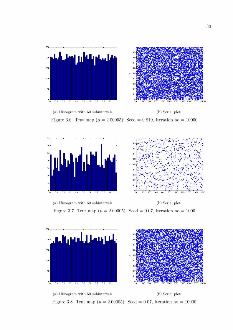
(a) Histogram with 50 subintervals (b) Serial plot
Figure 3.6: Tent map (µ = 2.00005): Seed = 0.819, Iteration no = 10000.
(a) Histogram with 50 subintervals (b) Serial plot
Figure 3.7: Tent map (µ = 2.00005): Seed = 0.07, Iteration no = 1000.
(a) Histogram with 50 subintervals (b) Serial plot
Figure 3.8: Tent map (µ = 2.00005): Seed = 0.07, Iteration no = 10000.

31
The results of the statistical tests of 20 sequences of numbers can be seen in the
Table 3.3 and Table 3.4. The first two columns of the tables are the statistical test
results of the sequences of numbers which have histograms, and serial plots above. As
shown in the tables, almost all p-values of tests are larger than 0.05. More than half
of the correlation coefficients are in the acceptable region for autocorrelation test.
Table 3.3: The statistical test results for 10 different seeds under tent map (µ =
2.00005): Iteration no = 1000.

32
Table 3.4: The statistical test results for 10 different seeds under tent map (µ =
2.00005): Iteration no = 10000.
3.3. Logistic Map (ν = 4)
Logistic map with parameter ν = 4 is the third suggested RNG. It is not
only a chaotic dynamical system but also a high-periodic map. It generates 1000000
numbers and more. We generate hundreds of sequences of 1000 and 10000 numbers
to understand the properties of logistic map. An interesting point for the histograms
of them is that they look like U-shape. In other words, the sequences of generated
numbers are not uniformly distributed, (see Figure 3.9). We need to transform the
sequences of generated numbers to the sequences of uniformly distributed numbers.
We obtain the natural invariant density of the logistic map by the derivation of
the transformation [0]. For x in the interval Λµ = [0, 1], define y, in Λν = [0, 1], by
x = sin2(πy
2) =
1
2[1− cos(πy)]. (3.1)

33
Figure 3.9: Histogram for logistic map.
The natural invariant density of the logistic map is derived easily
ρ(x) =
∣∣∣∣dydx∣∣∣∣ ρ(y)
where ρ(y) = 1. Since under Equation 3.1 y is shown to have uniform invariant density
[0]. One can easily compute that
ρ(x) =π−1
[x(1− x)]12
. (3.2)
The graph of Equation 3.2 can be seen in Figure 3.10. This graph and Figure 3.9
are very similar. This result implies that the logistic map does not uniformly distributed
on the interval [0, 1], and the transformation is necessary to have a uniformly distributed
function.
After the transformation, we get the sequences of numbers that are uniformly
distributed. The sequence of numbers used in Figure 3.9 transforms to the sequence of
numbers that is uniformly distributed, as seen in Figure 3.11. Now, we can take into
consideration the transformed sequences of numbers for logistic map. In the thesis,
we apply the transformation on the sequences of the numbers that are generated by
logistic map, and we call transformed logistic map as T-logistic map.

34
Figure 3.10: The graph of invariant density of logistic map
Figure 3.11: Histogram for transformed logistic map (T-logistic map).

35
The period of T-logistic map does not depend on seeds, and it can be more
than 1000000 numbers. The hundreds of seeds from [0, 1] are used in the randomness
tests of T-logistic map. For each seed, the sequences of 1000 and 10000 numbers
are produced, and transformed. The histograms of the sequences of the numbers are
acceptable to pass the uniformity tests. The serial plots of them imply the independence
of the numbers. They are also tested statistically. According to the tests results,
T-logistic map produces the sequences of random numbers.
We randomly select 10 different seeds. Ten of 1000-number-sequences and ten
of 10000-number-sequences are computed and transformed. The histograms and the
serial plots of 2 out of 10 sequences from each group are shown below in Figure 3.12-15.
The histograms and the serial plots of 16 sequences can be found in Appendix C.
(a) Histogram with 50 subintervals (b) Serial plot
Figure 3.12: T-logistic map (ν = 4): Seed = 0.774, Iteration no = 1000.
The results of eye test are also confirmed by statistical tests. We apply the
statistical tests into 20 sequences of numbers. Almost in all tests the null hypothesis is
rejected at the 5% significance level. The test results are affirmative. The results of the
statistical tests of 20 sequences can be seen in the Table 3.5, and Table 3.6. The first
two columns of the tables are the statistical test results of the sequences of numbers
which have histograms, and serial plots above. The test results show that T-logistic
map with parameter ν = 4 can be used as a RNG.
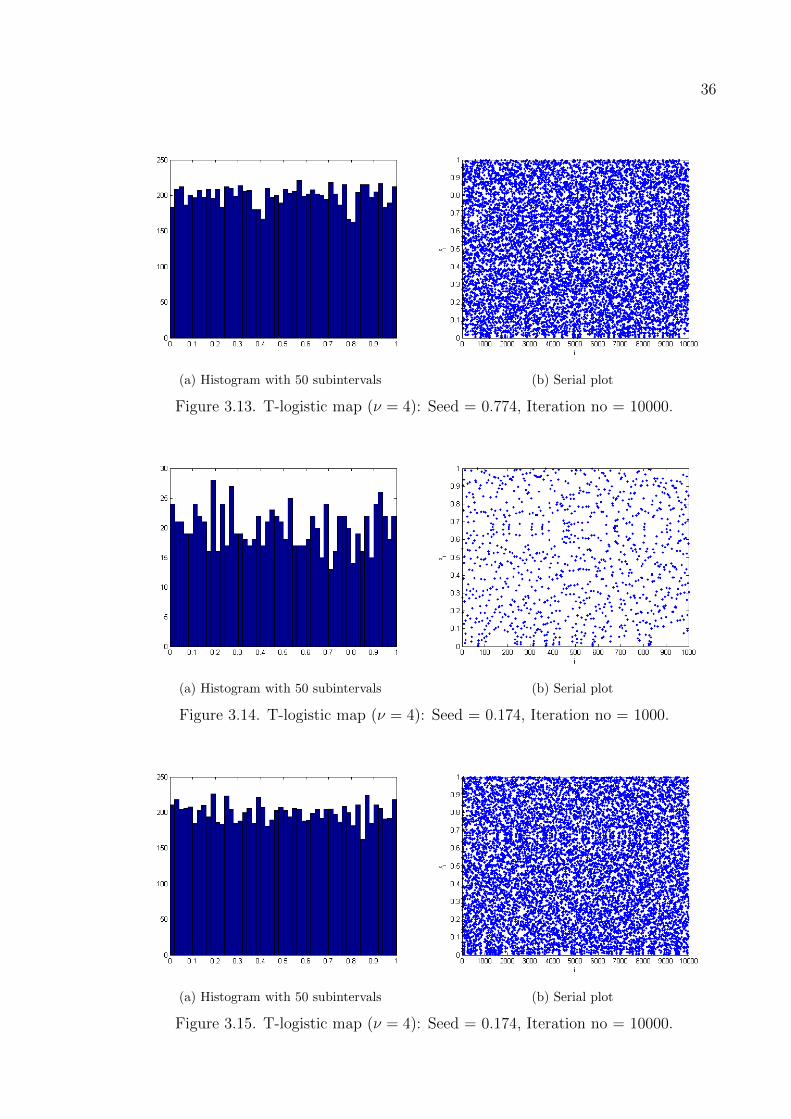
36
(a) Histogram with 50 subintervals (b) Serial plot
Figure 3.13: T-logistic map (ν = 4): Seed = 0.774, Iteration no = 10000.
(a) Histogram with 50 subintervals (b) Serial plot
Figure 3.14: T-logistic map (ν = 4): Seed = 0.174, Iteration no = 1000.
(a) Histogram with 50 subintervals (b) Serial plot
Figure 3.15: T-logistic map (ν = 4): Seed = 0.174, Iteration no = 10000.

37
Table 3.5: The statistical test results for 10 different seeds under T-logistic map (ν = 4):
Iteration no = 1000.
Table 3.6: The statistical test results for 10 different seeds under T-logistic map (ν = 4):
Iteration no = 10000.

38
3.4. Connecting Family of Maps (α = 0.999 and α = 1.01)
The last suggested RNGs are connecting family of mappings with parameters
α = 0.999 and α = 1.01. The first observation about the maps is the graphs of them.
They are similar to the graphs of the tent map with parameter µ = 2, as shown
in Figure 3.16. They have same properties as the tent map, except the relationship
between seed and period of the tent map. The periods of connecting maps are not
sensitive on seeds. Moreover, the periods of them become more than 1000000.
(a) C0.999 (b) C1.01
Figure 3.16: The graph of connecting maps (α = 0.999 and α = 1.01).
We generate hundreds of sequences of numbers, and observe histograms and serial
plots. All histograms confirm uniformity of the sequences of the numbers. Serial plots
illustrate that the numbers are independently spread on the xy-plane. The sequences
of numbers also pass the statistical tests. Almost all p-values of uniformity tests and
dependence tests are adequate that the connecting maps have random behavior.
We select 10 different seeds randomly and generate 20 sequences of numbers for
each parameter α = 0.999 and α = 1.01. The histograms and the serial plots of 2
out of 10 sequences from each group for α = 0.999 and α = 1.01 are shown in Figure
3.17-20 and Figure 3.21-24 respectively. The rest of histograms and serial plots of two
maps can be found in Appendix D and Appendix E.

39
(a) Histogram with 50 subintervals (b) Serial plot
Figure 3.17: Connecting map (α = 0.999): Seed = 0.727, Iteration no = 1000.
(a) Histogram with 50 subintervals (b) Serial plot
Figure 3.18: Connecting map (α = 0.999): Seed = 0.727, Iteration no = 10000.
(a) Histogram with 50 subintervals (b) Serial plot
Figure 3.19: Connecting map (α = 0.999): Seed = 0.819, Iteration no = 1000.

40
(a) Histogram with 50 subintervals (b) Serial plot
Figure 3.20: Connecting map (α = 0.999): Seed = 0.819, Iteration no = 10000.
(a) Histogram with 50 subintervals (b) Serial plot
Figure 3.21: Connecting map (α = 1.01): Seed = 0.0006, Iteration no = 1000.
(a) Histogram with 50 subintervals (b) Serial plot
Figure 3.22: Connecting map (α = 1.01): Seed = 0.0006, Iteration no = 10000.

41
(a) Histogram with 50 subintervals (b) Serial plot
Figure 3.23: Connecting map (α = 1.01): Seed = 0.8066, Iteration no = 1000.
(a) Histogram with 50 subintervals (b) Serial plot
Figure 3.24: Connecting map (α = 1.01): Seed = 0.8066, Iteration no = 10000.

42
We apply the statistical tests to 20 sequences of generated numbers. The results
of the statistical tests of 20 sequences can be seen in the Table 3.7, Table 3.8, Table 3.9,
and Table 3.10. The first two columns of the tables are the statistical test results of the
sequences of numbers which have histograms, and serial plots above. The connecting
family of mappings with parameters α = 0.999 and α = 1.01 pass randomness tests,
and uniformity tests.
Table 3.7: The statistical test results for 10 different seeds under connecting map
(α = 0.999): Iteration no = 1000.

43
Table 3.8: The statistical test results for 10 different seeds under connecting map
(α = 0.999): Iteration no = 10000.
Table 3.9: The statistical test results for 10 different seeds under connecting map
(α = 1.01): Iteration no = 1000.

44
Table 3.10: The statistical test results for 10 different seeds under connecting map
(α = 1.01): Iteration no = 10000.
3.5. Lyapunov Exponents Of The Suggested Maps
The Lyapunov exponent measures the rate of exponential divergence of nearby
points. In practice, it gives an idea about how fast a chaotic map becomes
unpredictable. If the Lyapunov exponent is ln(c) then we can expect an error
between two corresponding final points cnε after n iterations where ε was the initial
error between two starting points.
The computation of the Lyapunov exponent varies depending on the type of
the map: discrete maps and continuous maps. Since the suggested chaotic maps are
continuous functions on the interval [0, 1], Equation 3.3 is used in order to compute
the Lyapunov exponents (Λ) of the maps. The integral equation consists of two parts,
invariant density of map (ρ(x)) and logarithm of the derivative of map.
Λ =
∫ 1
0
ρ(x)ln∣∣∣f ′(x)
∣∣∣ dx (3.3)

45
For the Tent map f(x) = 1− |1− 2x|, the natural invariant density (ρ(x)) of the
map is known to be 1, [0]. The derivative of tent map (f′(x)) is equal to 2 if x < 1
2
and −2 otherwise. Therefore, the Lyapunov exponent of the tent map with parameter
µ = 2 is ln2 (∼= 0.69314).
For the tent map f(x) = 1 − |1− µx| with µ = 2.00005, we need to find the
invariant density of the map after applied IF method. This tent map consists of four
subintervals after IF method was applied, which are listed below.
f(x) =
2.00005x , 0 < x < 12.00005
−2.00005x+ 2 , 12.00005
< x < 12
2.00005x− 0.00005 , 12< x < 1.00005
2.00005
−2.00005x+ 2.00005 , 1.000052.00005
< x < 1
The stationary probabilities of each part are calculated in order to compute the
invariant density of the tent map. They are 0.499975001, 0.000012499, 0.000012499,
0.5 respectively for each interval. The natural invariant density of the tent map is:
ρ(x) =
0.4999750010.4999875
, 0 < x < 12.00005
0.0000124990.0000125
, 12.00005
< x < 12
0.0000124990.0000125
, 12< x < 1.00005
2.00005
0.50.4999875
, 1.000052.00005
< x < 1
The above function is thus very close to 1.
The derivative of this tent map is equal to 2.00005 if x < 12
and −2.00005
otherwise. So the integral equation becomes the multiplication of ln(2.00005) and
the integral of the invariant density. Since the integral of the density function is 1,
the Lyapunov exponent of the tent map with parameter µ = 2.00005 is ln(2.00005)
(∼= 0.69317).

46
For transformed logistic map (T-logistic map) f(x) = 1−|1− 2x|, it is equivalent
to the tent map with parameter µ = 2. That’s why the natural invariant density
of the T-logistic map is 1, and the Lyapunov exponent of the T-logistic map is ln2
(∼= 0.69314).
For the connecting maps f(x) = 1 − |1− 2x|α, the Lyapunov exponents of the
connecting maps with parameters α = 0.999 and α = 1.01 are not easily computed
due to the fact that there is no explicit function to represent the invariant densities of
the connecting maps. To determine the invariant densities of the connecting maps we
consider the histograms of the numbers that are generated by the connecting maps,
since the invariant density of a map is a function that fits to the histograms of the
numbers generated by map.
Firstly, we observe histograms of the generated numbers for two connecting maps.
As can be seen in the frequency histograms in Section 3.4, the invariant densities of
two connecting maps have uniformly distributed shapes, (also see Appendix D and E).
Secondly, we apply the statistical chi-square tests to the numbers generated by
these connecting maps. As can be seen in Section 3.4, ten 1000-number-sequences
and ten 10000-number-sequences for 10 different seeds are generated and chi-square
tests are applied to analyze the property of uniformity of the connecting maps. The
performances of the maps for chi-square tests are summarized in Table 3.11. The
table shows the number of chi-square tests passed with 10 different seeds under two
connecting maps where p-values of 0.05 is used as the test criteria.
Table 3.11: Number of chi-square tests passed with 10 different seeds for two connecting
maps (p-values of 0.05 is used as the test criteria).
Iteration no = 1000 Iteration no = 10000
Statistical Tests α = 0.999 α = 1.01 α = 0.999 α = 1.01
Total # of passes in
10 Chisquare Tests8 10 8 9
Passing Success 80.0% 100.0% 80.0% 90.0%

47
In Section 4.2, more test results comparing the uniformities of connecting maps
versus linear congruential generators are provided. In conclusion, we can assume that
invariant density of these connecting maps is approximately 1.
The Lyapunov exponent of the connecting maps with parameter α = 1.01 is next
computed:
Λ =
∫ 1
0
ρ(x)ln∣∣∣f ′(x)
∣∣∣ dx=
∫ 1
0
ln∣∣2(1.01)(1− 2x)0.01
∣∣ dx= ln(2.02) +
∫ 1
0
ln∣∣(1− 2x)0.01
∣∣ dx= ln(2.02) +
∫ 12
0
ln((1− 2x)0.01)dx+
∫ 1
12
ln((2x− 1)0.01)dx
= ln(2.02) + (0.01)
∫ 12
0
ln(1− 2x)dx+ (0.01)
∫ 1
12
ln(2x− 1)dx
= ln(2.02) + (0.01)1
2
∫ 1
0
ln(u)du+ (0.01)1
2
∫ 1
0
ln(u)du
= ln(2.02) + (0.01) [uln(u)− u]10
= ln(2.02)− (0.01) ∼= 0.69309.

48
The Lyapunov exponent of the connecting maps with parameter α = 0.999 is
computed:
Λ =
∫ 1
0
ρ(x)ln∣∣∣f ′(x)
∣∣∣ dx=
∫ 1
0
ln∣∣2(0.999)(1− 2x)−0.001
∣∣ dx= ln(1.998) +
∫ 1
0
ln∣∣(1− 2x)−0.001
∣∣ dx= ln(1.998) +
∫ 12
0
ln((1− 2x)−0.001)dx+
∫ 1
12
ln((2x− 1)−0.001)dx
= ln(1.998)− (0.001)
∫ 12
0
ln(1− 2x)dx− (0.001)
∫ 1
12
ln(2x− 1)dx
= ln(1.998)− (0.001)1
2
∫ 1
0
ln(u)du− (0.001)1
2
∫ 1
0
ln(u)du
= ln(1.998)− (0.001) [uln(u)− u]10
= ln(1.998) + (0.001) ∼= 0.69314.
To conclude, the Lyapunov exponents of all suggested maps are exactly or
approximately 0.6931 ( ∼= ln2). If the initial error between two points is ε = 10−16,
then the error 2nε is approximately equal to 1 after n = 53 iterations.
49
4. COMPARISON BETWEEN FIVE SUGGESTED
CHAOTIC MAPS AND SOME WELL-KNOWN LINEAR
CONGRUENTIAL GENERATORS (LCGs)
4.1. Linear Congruential Generators (LCGs)
In this part of the thesis, we will compare our five suggested chaotic maps with
some well-known linear congruential generators (LCGs). We would like to choose LCGs
that are conventionally used in many areas. Five different LCGs are selected for the
comparison. Two of them are multiplicative linear congruential generators (MLCGs),
and the other ones are linear congruential generators (LCGs), as listed in Table 4.1.
These generators are actively used in Borland C/C++, CodeWarrior, IBM VisualAge
C/C++, Apple CarbonLib, Borland Delphi, and Virtual Pascal. It is necessary to
compare five suggested chaotic maps with the well-known LCGs to understand whether
they are successful in generating of random numbers or not. If they are as successful
as LCGs, then we can approve the actual use of them as RNGs.
LCGs produces a sequence of integers, X1, X2, ... between 0 and m−1 by following
a recursive relation:
Xn+1 = (aXn + c) modm, i = 0, 1, 2, ...
They are defined from the set of integers {0, 1, 2, ...,m− 1} to the set of integers
{0, 1, 2, ...,m− 1}, but the five suggested RNGs are defined from [0, 1] to [0, 1]. For
meaningful results, we convert the chosen integer seeds for LCGs to real numbers in
[0, 1]. For the conversion, the chosen integer seeds for LCGs are divided by multiples
of 10. For instance, X0 = 123, 457 converts to X0 = 0.00123457 for tent map with
parameter µ = 2, and X0 = 0.123457 for the other four maps. (The reason of keeping
tent map with parameter µ = 2 separate are explained in the previous chapter.) The

50
largest possible periods (P ) of LCGs can be calculated by the choice of a, c, m and
X0, [2].
Table 4.1: List of some well-known linear congruential generators (LCGs).
Source a m c P
MLCG 1 - 742938285 231 − 1 0 231 − 2
MLCG 2 Apple CarbonLib 16807 231 − 1 0 231 − 2
LCG 3 Borland C/C++ 22695477 232 1 232
LCG 4 CodeWarrior, 1103515245 232 12345 232
IBM VisualAge C/C++
LCG 5 Microsoft Visual, 214013 232 2531011 232
Quick C/C++
Before starting the comparison, we observe the histograms and serial plots of
the sequences of numbers generated by LCGs. We take two randomly selected seeds
for each LCG, and generate ten of 1000-number-sequences and ten of 10000-number-
sequences. The histograms and serial plots for LCGs are shown in Figure 4.1-20.
(a) Histogram with 50 subintervals (b) Serial plot
Figure 4.1: MLCG 1: Seed = 931, Iteration no = 1000.

51
(a) Histogram with 50 subintervals (b) Serial plot
Figure 4.2: MLCG 1: Seed = 931, Iteration no = 10000.
(a) Histogram with 50 subintervals (b) Serial plot
Figure 4.3: MLCG 1: Seed = 6647, Iteration no = 1000.
(a) Histogram with 50 subintervals (b) Serial plot
Figure 4.4: MLCG 1: Seed = 6647, Iteration no = 10000.

52
Table 4.2: The statistical test results for two different seeds under MLCG 1.
(a) Histogram with 50 subintervals (b) Serial plot
Figure 4.5: MLCG 2: Seed = 13, Iteration no = 1000.
(a) Histogram with 50 subintervals (b) Serial plot
Figure 4.6: MLCG 2: Seed = 13, Iteration no = 10000.

53
(a) Histogram with 50 subintervals (b) Serial plot
Figure 4.7: MLCG 2: Seed = 36509, Iteration no = 1000.
(a) Histogram with 50 subintervals (b) Serial plot
Figure 4.8: MLCG 2: Seed = 36509, Iteration no = 10000.
Table 4.3: The statistical test results for two different seeds under MLCG 2.

54
(a) Histogram with 50 subintervals (b) Serial plot
Figure 4.9: LCG 3: Seed = 1637, Iteration no = 1000.
(a) Histogram with 50 subintervals (b) Serial plot
Figure 4.10: LCG 3: Seed = 1637, Iteration no = 10000.
(a) Histogram with 50 subintervals (b) Serial plot
Figure 4.11: LCG 3: Seed = 5161, Iteration no = 1000.
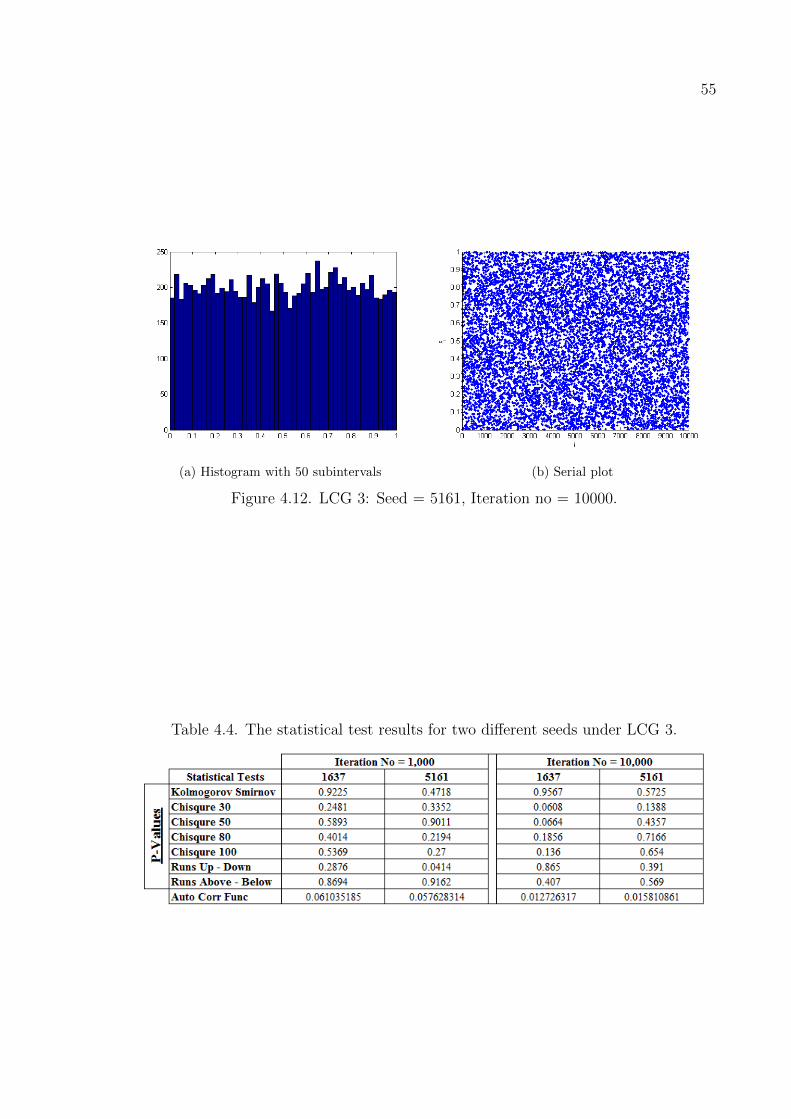
55
(a) Histogram with 50 subintervals (b) Serial plot
Figure 4.12: LCG 3: Seed = 5161, Iteration no = 10000.
Table 4.4: The statistical test results for two different seeds under LCG 3.
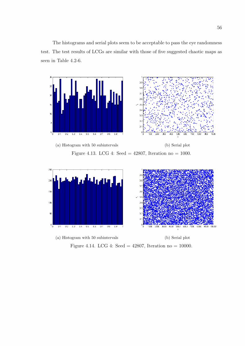
56
The histograms and serial plots seem to be acceptable to pass the eye randomness
test. The test results of LCGs are similar with those of five suggested chaotic maps as
seen in Table 4.2-6.
(a) Histogram with 50 subintervals (b) Serial plot
Figure 4.13: LCG 4: Seed = 42807, Iteration no = 1000.
(a) Histogram with 50 subintervals (b) Serial plot
Figure 4.14: LCG 4: Seed = 42807, Iteration no = 10000.

57
(a) Histogram with 50 subintervals (b) Serial plot
Figure 4.15: LCG 4: Seed = 11, Iteration no = 1000.
(a) Histogram with 50 subintervals (b) Serial plot
Figure 4.16: LCG 4: Seed = 11, Iteration no = 10000.
Table 4.5: The statistical test results for two different seeds under LCG 4.

58
(a) Histogram with 50 subintervals (b) Serial plot
Figure 4.17: LCG 5: Seed = 6625, Iteration no = 1000.
(a) Histogram with 50 subintervals (b) Serial plot
Figure 4.18: LCG 5: Seed = 6625, Iteration no = 10000.
(a) Histogram with 50 subintervals (b) Serial plot
Figure 4.19: LCG 5: Seed = 87, Iteration no = 1000.
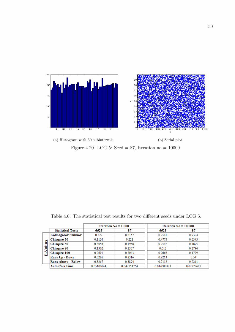
59
(a) Histogram with 50 subintervals (b) Serial plot
Figure 4.20: LCG 5: Seed = 87, Iteration no = 10000.
Table 4.6: The statistical test results for two different seeds under LCG 5.

60
4.2. Basic Comparison of Five Suggested Chaotic Maps and LCGs
We test the performance of five suggested chaotic maps and LCGs. We use
the seeds which are suggested by developers and actual users of LCGs. 20 suggested
different seeds are selected. Using these seeds, we run LCGs and the five suggested maps
to generate 1000-number-sequences and 10000-number-sequences. For each seed, there
are 20 different 1000-number-sequences and 10000-number-sequences
individually, generated by 10 different maps.
The first step is to observe histograms and serial plots of the sequences of numbers.
We scan 400 different histograms and serial plots, and all of them are good enough to
pass the eye test. Furthermore there is no significant difference between histograms
and serial plots of the sequences of numbers. Twenty of 400 figures are provided in
Appendix F and G.
The second step is the statistical tests. Kolmogorov Smirnov test and chi square
test are applied to compare the property of uniformity of the maps with each other.
Runs tests and autocorrelation test are taken into account to examine independence
property in each sequence of generated numbers. The test results of the sequences of
numbers for one of 20 seeds is listed below, (see Table 4.7 and Table 4.8). Although
the numbers of tests passed by LCGs are larger than ones by the five suggested chaotic
maps, there is no significant difference between the test results. When these results
are taken into account for the usability of the five chaotic maps as RNGs, they are as
successful as LCGs. The test results of the sequences of numbers for 19 seeds can be
found in Appendix H, I, J and K.
The overall performances of the tests are summarized in Table 4.9. The table
shows the number of tests passed with 20 different seeds under LGCs and five suggested
maps where p-values of 0.05 and the related confidence bounds, which are ±0.0632 and
±0.02 for the sample sizes 1000 and 10000 respectively, are used as the test criteria.
We consider Kolmogorov-Smirnov test and chi-square test for uniformity tests, and
autocorrelation test for serial test for each map. Test results are over 20 for each test,

61
Table 4.7: The statistical test results for LGCs and five suggested maps: Seed =
3316779, Iteration no = 1000.
Table 4.8: The statistical test results for LGCs and five suggested maps: Seed =
3316779, Iteration no = 10000.

62
and the sum of these results can be 60 at most.
LCGs seem to be somewhat more successful than the chaotic RNGs in statistical
tests. Tent map with parameter µ = 2.00005 and MLCG 2 reach success ratios of 90%
and 95% respectively, which are the highest ratios of the tests, when the number of
iterations is 1000. The minimum ratios are observed for T-logistic map and MLCG 1,
which are 75% and 85%. Overall average success rate of five suggested maps in tests
is 81%, and it is observed for LCGs as 90.3%.
When the number of iterations is 10000, the five suggested chaotic maps reach the
highest ratio at 85%. The highest ratio for LCGs is 86.7% in this case. The minimum
ratios of five suggested maps and LCGs are seen as 80% and 83.3% for connecting map
with the parameter α = 1.01 and LCG 5 respectively. Overall average success rate of
five suggested chaotic maps in tests is 83.3%, whereas it is 87.7% for LCGs, (see Table
4.9).
Table 4.9: Number of tests passed with 20 different seeds under LGCs and five sug-
gested maps (p-values of 0.05 is used as the test criteria).
These test ratios increase when p-values of 0.01 and the related confidence bounds,
which are ±0.0948 and ±0.03 for the sample sizes 1000 and 10000 respectively, are used
as the test criteria. The highest success ratios of 100% and of 98.3% are observed for
five suggested maps and LCGs respectively when the number of iterations is taken as
1000. The minimum ratios become 90% for five suggested maps, and 96.7% for LCGs.

63
Overall average success rate of five suggested chaotic maps in tests is 96.7%, and it is
observed for LCGs as 97.7%.
When iteration number is 10000, a decrement is observed in the highest ratio for
five suggested chaotic maps. It decreases to 98.3%. However there is an increment
in the lowest ratio for them. It is observed as 93.3% for them. The highest ratio of
LCGs increases to 100%, and the lowest ratio of them reach to 98.3% in this situation.
Overall average success rate of five suggested chaotic maps and LCGs in tests become
95.7% and 99.7% respectively, (see Table 4.10).
Table 4.10: Number of tests passed with 20 different seeds under LGCs and five sug-
gested maps (p-values of 0.01 is used as the test criteria).

64
4.3. Further Analysis and Comparisons of the Suggested Chaotic Maps
We consider five suggested chaotic maps and LCGs. The five chaotic maps pass
statistical tests satisfactorily, (see Table 4.9 and Table 4.10). These results support the
idea that the chaotic maps can generate random numbers like LCGs.
In the empirical tests, we consider histograms and serial plots for the generated
numbers for each map. Histograms show the frequencies of the generated numbers,
and serial plots illustrate the relations between the iteration number and the generated
numbers (n, xn).
For further analysis of the generated random numbers, we plot the graphs of
two consecutive iterated numbers (xn, xn+1). We take a seed, which is used in the
comparison section 4.2, and generate 1000 numbers to plot (xn, xn+1) graph of each
map. The graphs can be seen in Figure 4.21 and Figure 4.22 for chaotic maps and
LCGs respectively, and the statistical test results of the generated numbers can be
seen in Table 4.11.

65
(a) Tent Map (µ = 2) (b) Tent Map (µ = 2.00005)
(c) T-logistic Map (ν = 4)
(d) Connecting Map (α = 0.999) (e) Connecting Map (α = 1.01)
Figure 4.21: The (xn, xn+1) graphs of chaotic maps.

66
(a) MLCM1 (b) MLCM2
(c) LCM3 (d) LCM4
(e) LCM5
Figure 4.22: The (xn, xn+1) graph of LCGs.

67
The figures show that the numbers generated by LCGs diffuse randomly in
(xn, xn+1) plane. This situation results from the modulus operation inside LCGs.
When chaotic maps are examined, the generated numbers draw the graphs of related
equations, which are obviously not random. Although the generated numbers are not
randomly distributed in (xn, xn+1) plane, the nature of chaotic dynamical maps do
contain strong unpredictability. Due to the property of chaotic maps, the generated
numbers are randomly distributed in (n, xn) plane and pass the related randomness
tests (as already seen in Section 4.2).
Table 4.11: The statistical test results for LCGs and five suggested maps: Seed =
915612027, Iteration no = 1000.
The unpredictability property of chaotic maps is so strong that they generate
randomly distributed numbers in (n, xn) plane. In order to obtain randomness in
(xn, xn+1) plane as well, using modulus operation with chaotic maps to generate random
numbers will probably produce better results. Such generated numbers may produce
independence test results as those of LCGs. The use of such chaotic maps with modulus
operations as RNGs can be a further research topic.

68
5. CONCLUSION
This thesis deals with the generation of pseudo random numbers (PRNs) by
means of chaotic dynamical maps. The nature of a chaotic dynamical map contains
unpredictability itself, a motivation behind our thesis study. The research question is:
to what extent some chaotic dynamical maps can be used in the generation of random
numbers.
We develop five different random number generators (RNGs) that are based on
five different chaotic dynamical maps. In three steps, we check the performances of five
suggested chaotic maps as RNGs.
Firstly, the periods of five suggested maps are controlled. Conditions that
guarantee the generation of more than 1000000 numbers without any cycles are deter-
mined for each chaotic map. After it is confirmed that each map can generate 1000000
numbers at least, the sequences of 1000 and 10000 numbers are generated as samples
in order to test the uniformity and randomness of each map.
Secondly, the histograms and the serial plots of the sequences of generated
numbers are examined visually as a first test. Such graphs give an idea about the
randomness of the maps. We check uniformity of the generated numbers visually with
their histograms, and independence of the sequences of these numbers with serial plots.
It is observed that the suggested RNGs perform well according to visual tests.
Thirdly, the generated numbers are tested by Kolmogorov Smirnov test, and
chi-square test to assess their properties of uniformity. (Chi-square tests are run for
different numbers of classes: 30, 50, 80, and 100). Runs tests (runs up and down
test, and runs above and below mean test), and autocorrelation tests are next applied
to the sequences of generated numbers to test their independence property. The five
suggested maps performed well in all these tests, and uniformity and independence of
the sequences of the generated numbers are confirmed.

69
We finally compare our suggested maps with some best known linear congruential
generators (LCGs). We select 20 different seeds that conform the desired properties of
LCGs for the comparison of LCGs and five suggested chaotic RNGs. The visual tests
and statistical tests are both taken into account. No undesirable patterns are observed
in visual tests for any of the generators. In statistical tests, we compare the test results
of LCGs and five suggested maps.
LCGs perform well since they are already suggested as some of the best generators
in the literature and the seeds satisfy some suggested specific conditions. (ie. the seeds
are all prime or odd numbers.) However, the five suggested chaotic dynamical maps
perform almost as well as LCGs. Similarly the performance of five suggested chaotic
RNGs can be improved through defining seeds that perform well for these five RNGs.
To sum up, we propose that our five chaotic dynamical maps can be potentially
used as random number generators. These suggested random number generators have
only one simple chaotic function each, so they are practical and efficient.
The use of such chaotic maps as RNGs can be further studied by investigating
the relation between seeds used and the resulting random number properties. More
detailed mathematical, statistical and numerical properties of the suggested generators
also constitute useful further research topics. As another further research topic in order
to improve performance of suggested chaotic generators, the use of modulus operations
with suggested chaotic generators can be analyzed.

70
APPENDIX A: HISTOGRAMS FOR TENT MAP (µ = 2)
(a) Histogram with 50 subintervals (b) Serial plot
Figure A.1: Tent map (µ = 2): Seed = 0.197600506499, Iteration no = 1000.
(a) Histogram with 50 subintervals (b) Serial plot
Figure A.2: Tent map (µ = 2): Seed = 0.197600506499, Iteration no = 10000.

71
(a) Histogram with 50 subintervals (b) Serial plot
Figure A.3: Tent map (µ = 2): Seed = 0.231069988461, Iteration no = 1000.
(a) Histogram with 50 subintervals (b) Serial plot
Figure A.4: Tent map (µ = 2): Seed = 0.231069988461, Iteration no = 10000.
(a) Histogram with 50 subintervals (b) Serial plot
Figure A.5: Tent map (µ = 2): Seed = 0.98388083416, Iteration no = 1000.

72
(a) Histogram with 50 subintervals (b) Serial plot
Figure A.6: Tent map (µ = 2): Seed = 0.98388083416, Iteration no = 10000.
(a) Histogram with 50 subintervals (b) Serial plot
Figure A.7: Tent map (µ = 2): Seed = 0.389913876011, Iteration no = 1000.
(a) Histogram with 50 subintervals (b) Serial plot
Figure A.8: Tent map (µ = 2): Seed = 0.389913876011, Iteration no = 10000.

73
(a) Histogram with 50 subintervals (b) Serial plot
Figure A.9: Tent map (µ = 2): Seed = 0.455019664777, Iteration no = 1000.
(a) Histogram with 50 subintervals (b) Serial plot
Figure A.10: Tent map (µ = 2): Seed = 0.455019664777, Iteration no = 10000.
(a) Histogram with 50 subintervals (b) Serial plot
Figure A.11: Tent map (µ = 2): Seed = 0.490444465331, Iteration no = 1000.

74
(a) Histogram with 50 subintervals (b) Serial plot
Figure A.12: Tent map (µ = 2): Seed = 0.490444465331, Iteration no = 10000.
(a) Histogram with 50 subintervals (b) Serial plot
Figure A.13: Tent map (µ = 2): Seed = 0.086948882143, Iteration no = 1000.
(a) Histogram with 50 subintervals (b) Serial plot
Figure A.14: Tent map (µ = 2): Seed = 0.086948882143, Iteration no = 10000.
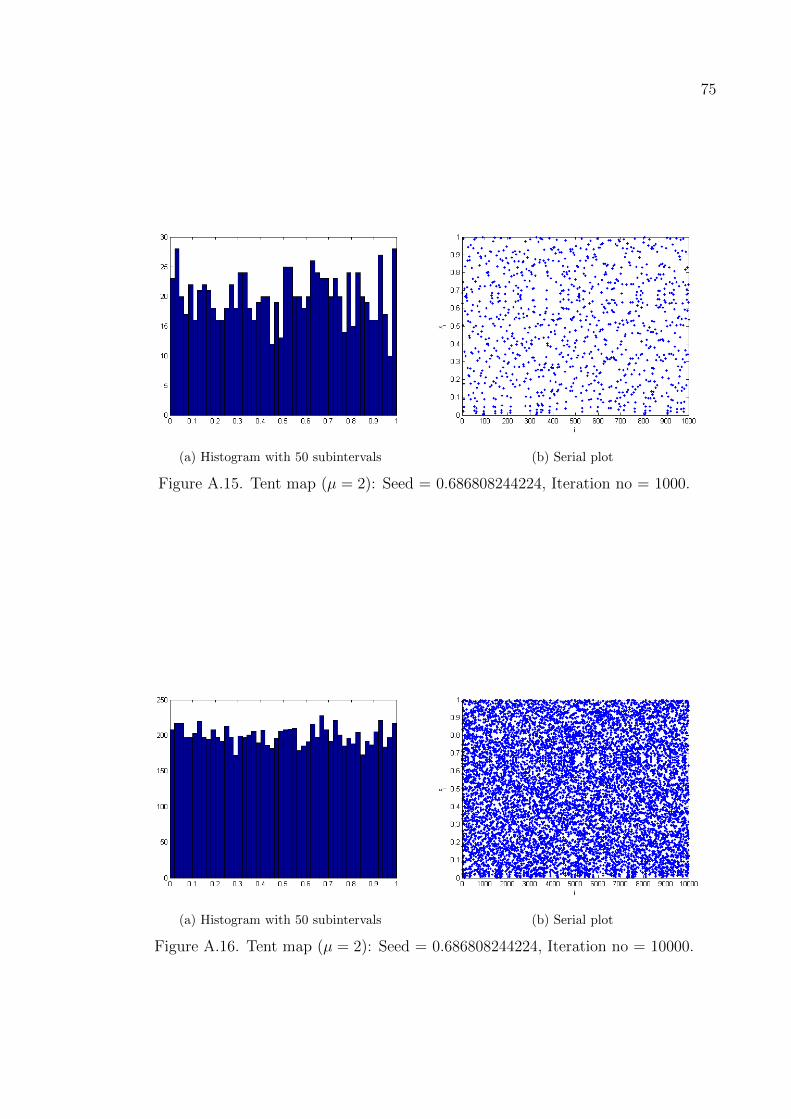
75
(a) Histogram with 50 subintervals (b) Serial plot
Figure A.15: Tent map (µ = 2): Seed = 0.686808244224, Iteration no = 1000.
(a) Histogram with 50 subintervals (b) Serial plot
Figure A.16: Tent map (µ = 2): Seed = 0.686808244224, Iteration no = 10000.

76
APPENDIX B: HISTOGRAMS FOR TENT MAP
(µ = 2.00005)
(a) Histogram with 50 subintervals (b) Serial plot
Figure B.1: Tent map (µ = 2.00005): Seed = 0.945195357852, Iteration no = 1000.
(a) Histogram with 50 subintervals (b) Serial plot
Figure B.2: Tent map (µ = 2.00005): Seed = 0.945195357852, Iteration no = 10000.

77
(a) Histogram with 50 subintervals (b) Serial plot
Figure B.3: Tent map (µ = 2.00005): Seed = 0.005382078128663, Iteration no = 1000.
(a) Histogram with 50 subintervals (b) Serial plot
Figure B.4: Tent map (µ = 2.00005): Seed = 0.005382078128663, Iteration no = 10000.
(a) Histogram with 50 subintervals (b) Serial plot
Figure B.5: Tent map (µ = 2.00005): Seed = 0.385874582044063, Iteration no = 1000.

78
(a) Histogram with 50 subintervals (b) Serial plot
Figure B.6: Tent map (µ = 2.00005): Seed = 0.385874582044063, Iteration no = 10000.
(a) Histogram with 50 subintervals (b) Serial plot
Figure B.7: Tent map (µ = 2.00005): Seed = 0.991, Iteration no = 1000.
(a) Histogram with 50 subintervals (b) Serial plot
Figure B.8: Tent map (µ = 2.00005): Seed = 0.991, Iteration no = 10000.

79
(a) Histogram with 50 subintervals (b) Serial plot
Figure B.9: Tent map (µ = 2.00005): Seed = 0.517, Iteration no = 1000.
(a) Histogram with 50 subintervals (b) Serial plot
Figure B.10: Tent map (µ = 2.00005): Seed = 0.517, Iteration no = 10000.
(a) Histogram with 50 subintervals (b) Serial plot
Figure B.11: Tent map (µ = 2.00005): Seed = 0.197600506499, Iteration no = 1000.

80
(a) Histogram with 50 subintervals (b) Serial plot
Figure B.12: Tent map (µ = 2.00005): Seed = 0.197600506499, Iteration no = 10000.
(a) Histogram with 50 subintervals (b) Serial plot
Figure B.13: Tent map (µ = 2.00005): Seed = 0.267781590398, Iteration no = 1000.
(a) Histogram with 50 subintervals (b) Serial plot
Figure B.14: Tent map (µ = 2.00005): Seed = 0.267781590398, Iteration no = 10000.

81
(a) Histogram with 50 subintervals (b) Serial plot
Figure B.15: Tent map (µ = 2.00005): Seed = 0.897496645632, Iteration no = 1000.
(a) Histogram with 50 subintervals (b) Serial plot
Figure B.16: Tent map (µ = 2.00005): Seed = 0.897496645632, Iteration no = 10000.

82
APPENDIX C: HISTOGRAMS FOR T-LOGISTIC MAP
(ν = 4)
(a) Histogram with 50 subintervals (b) Serial plot
Figure C.1: T-logistic map (ν = 4): Seed = 0.973, Iteration no = 1000.
(a) Histogram with 50 subintervals (b) Serial plot
Figure C.2: T-logistic map (ν = 4): Seed = 0.973, Iteration no = 10000.

83
(a) Histogram with 50 subintervals (b) Serial plot
Figure C.3: T-logistic map (ν = 4): Seed = 0.912091805655299, Iteration no = 1000.
(a) Histogram with 50 subintervals (b) Serial plot
Figure C.4: T-logistic map (ν = 4): Seed = 0.912091805655299, Iteration no = 10000.
(a) Histogram with 50 subintervals (b) Serial plot
Figure C.5: T-logistic map (ν = 4): Seed = 0.68, Iteration no = 1000.
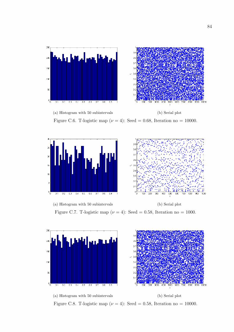
84
(a) Histogram with 50 subintervals (b) Serial plot
Figure C.6: T-logistic map (ν = 4): Seed = 0.68, Iteration no = 10000.
(a) Histogram with 50 subintervals (b) Serial plot
Figure C.7: T-logistic map (ν = 4): Seed = 0.58, Iteration no = 1000.
(a) Histogram with 50 subintervals (b) Serial plot
Figure C.8: T-logistic map (ν = 4): Seed = 0.58, Iteration no = 10000.

85
(a) Histogram with 50 subintervals (b) Serial plot
Figure C.9: T-logistic map (ν = 4): Seed = 0.282, Iteration no = 1000.
(a) Histogram with 50 subintervals (b) Serial plot
Figure C.10: T-logistic map (ν = 4): Seed = 0.282, Iteration no = 10000.
(a) Histogram with 50 subintervals (b) Serial plot
Figure C.11: T-logistic map (ν = 4): Seed = 0.4, Iteration no = 1000.

86
(a) Histogram with 50 subintervals (b) Serial plot
Figure C.12: T-logistic map (ν = 4): Seed = 0.4, Iteration no = 10000.
(a) Histogram with 50 subintervals (b) Serial plot
Figure C.13: T-logistic map (ν = 4): Seed = 0.758167338031333, Iteration no = 1000.
(a) Histogram with 50 subintervals (b) Serial plot
Figure C.14: T-logistic map (ν = 4): Seed = 0.758167338031333, Iteration no = 10000.

87
(a) Histogram with 50 subintervals (b) Serial plot
Figure C.15: T-logistic map (ν = 4): Seed = 0.809, Iteration no = 1000.
(a) Histogram with 50 subintervals (b) Serial plot
Figure C.16: T-logistic map (ν = 4): Seed = 0.809, Iteration no = 10000.

88
APPENDIX D: HISTOGRAMS FOR CONNECTING MAP
(α = 0.999)
(a) Histogram with 50 subintervals (b) Serial plot
Figure D.1: Connecting map (α = 0.999): Seed = 0.1, Iteration no = 1000.
(a) Histogram with 50 subintervals (b) Serial plot
Figure D.2: Connecting map (α = 0.999): Seed = 0.1, Iteration no = 10000.
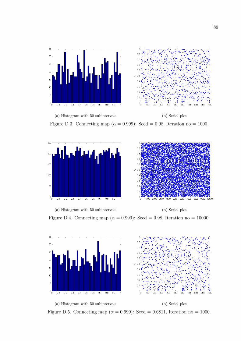
89
(a) Histogram with 50 subintervals (b) Serial plot
Figure D.3: Connecting map (α = 0.999): Seed = 0.98, Iteration no = 1000.
(a) Histogram with 50 subintervals (b) Serial plot
Figure D.4: Connecting map (α = 0.999): Seed = 0.98, Iteration no = 10000.
(a) Histogram with 50 subintervals (b) Serial plot
Figure D.5: Connecting map (α = 0.999): Seed = 0.6811, Iteration no = 1000.

90
(a) Histogram with 50 subintervals (b) Serial plot
Figure D.6: Connecting map (α = 0.999): Seed = 0.6811, Iteration no = 10000.
(a) Histogram with 50 subintervals (b) Serial plot
Figure D.7: Connecting map (α = 0.999): Seed = 0.002, Iteration no = 1000.
(a) Histogram with 50 subintervals (b) Serial plot
Figure D.8: Connecting map (α = 0.999): Seed = 0.002, Iteration no = 10000.

91
(a) Histogram with 50 subintervals (b) Serial plot
Figure D.9: Connecting map (α = 0.999): Seed = 0.7, Iteration no = 1000.
(a) Histogram with 50 subintervals (b) Serial plot
Figure D.10: Connecting map (α = 0.999): Seed = 0.7, Iteration no = 10000.
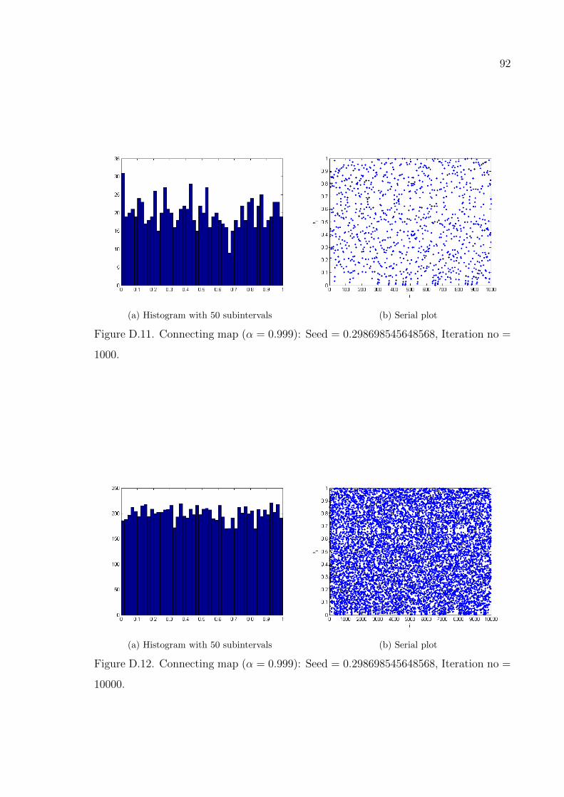
92
(a) Histogram with 50 subintervals (b) Serial plot
Figure D.11: Connecting map (α = 0.999): Seed = 0.298698545648568, Iteration no =
1000.
(a) Histogram with 50 subintervals (b) Serial plot
Figure D.12: Connecting map (α = 0.999): Seed = 0.298698545648568, Iteration no =
10000.

93
(a) Histogram with 50 subintervals (b) Serial plot
Figure D.13: Connecting map (α = 0.999): Seed = 0.525620161505902, Iteration no =
1000.
(a) Histogram with 50 subintervals (b) Serial plot
Figure D.14: Connecting map (α = 0.999): Seed = 0.525620161505902, Iteration no =
10000.

94
(a) Histogram with 50 subintervals (b) Serial plot
Figure D.15: Connecting map (α = 0.999): Seed = 0.333, Iteration no = 1000.
(a) Histogram with 50 subintervals (b) Serial plot
Figure D.16: Connecting map (α = 0.999): Seed = 0.333, Iteration no = 10000.

95
APPENDIX E: HISTOGRAMS FOR CONNECTING MAP
(α = 1.01)
(a) Histogram with 50 subintervals (b) Serial plot
Figure E.1: Connecting map (α = 1.01): Seed = 0.672551918078352, Iteration no =
1000.
(a) Histogram with 50 subintervals (b) Serial plot
Figure E.2: Connecting map (α = 1.01): Seed = 0.672551918078352, Iteration no =
10000.

96
(a) Histogram with 50 subintervals (b) Serial plot
Figure E.3: Connecting map (α = 1.01): Seed = 0.189, Iteration no = 1000.
(a) Histogram with 50 subintervals (b) Serial plot
Figure E.4: Connecting map (α = 1.01): Seed = 0.189, Iteration no = 10000.
(a) Histogram with 50 subintervals (b) Serial plot
Figure E.5: Connecting map (α = 1.01): Seed = 0.747, Iteration no = 1000.

97
(a) Histogram with 50 subintervals (b) Serial plot
Figure E.6: Connecting map (α = 1.01): Seed = 0.747, Iteration no = 10000.
(a) Histogram with 50 subintervals (b) Serial plot
Figure E.7: Connecting map (α = 1.01): Seed = 0.880223477310122, Iteration no =
1000.

98
(a) Histogram with 50 subintervals (b) Serial plot
Figure E.8: Connecting map (α = 1.01): Seed = 0.880223477310122, Iteration no =
10000.
(a) Histogram with 50 subintervals (b) Serial plot
Figure E.9: Connecting map (α = 1.01): Seed = 0.9, Iteration no = 1000.

99
(a) Histogram with 50 subintervals (b) Serial plot
Figure E.10: Connecting map (α = 1.01): Seed = 0.9, Iteration no = 10000.
(a) Histogram with 50 subintervals (b) Serial plot
Figure E.11: Connecting map (α = 1.01): Seed = 0.361436078541452, Iteration no =
1000.

100
(a) Histogram with 50 subintervals (b) Serial plot
Figure E.12: Connecting map (α = 1.01): Seed = 0.361436078541452, Iteration no =
10000.
(a) Histogram with 50 subintervals (b) Serial plot
Figure E.13: Connecting map (α = 1.01): Seed = 0.6001, Iteration no = 1000.
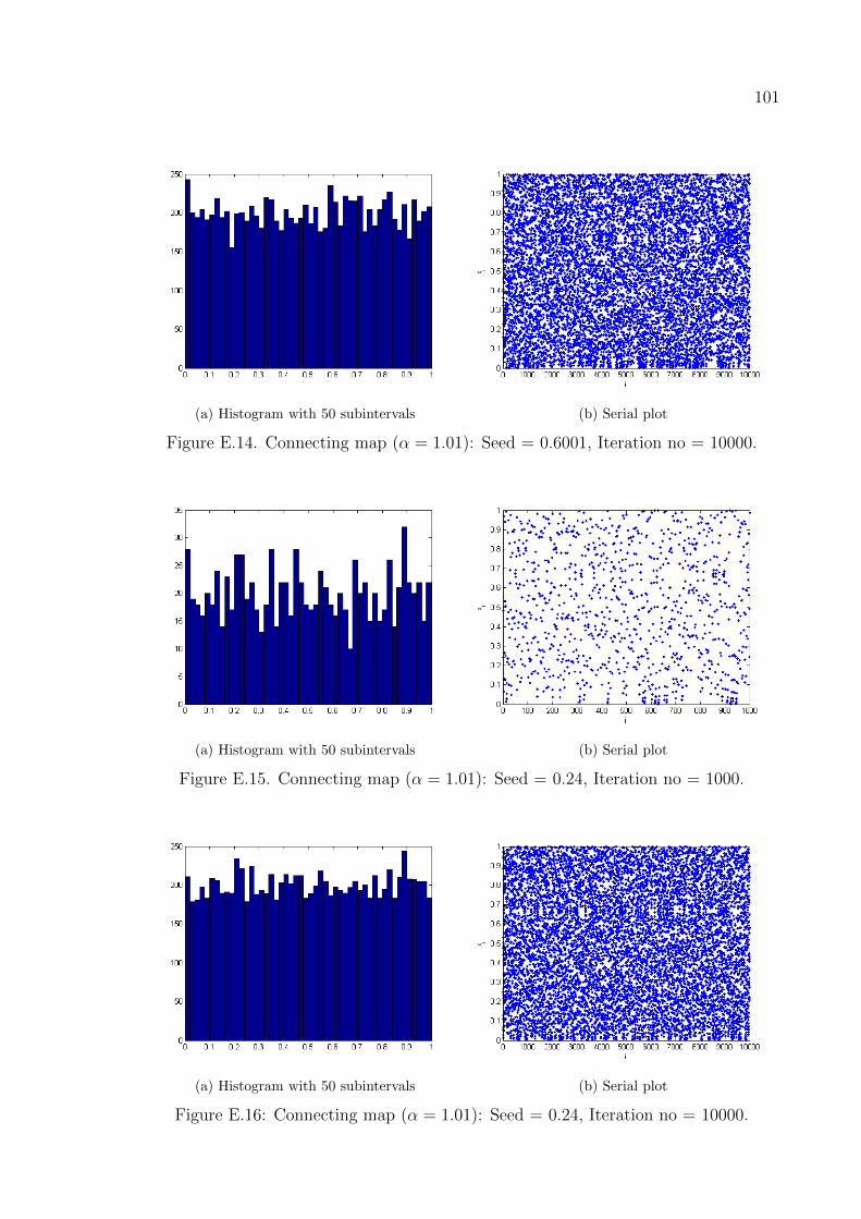
101
(a) Histogram with 50 subintervals (b) Serial plot
Figure E.14: Connecting map (α = 1.01): Seed = 0.6001, Iteration no = 10000.
(a) Histogram with 50 subintervals (b) Serial plot
Figure E.15: Connecting map (α = 1.01): Seed = 0.24, Iteration no = 1000.
(a) Histogram with 50 subintervals (b) Serial plot
Figure E.16: Connecting map (α = 1.01): Seed = 0.24, Iteration no = 10000.

102
APPENDIX F: HISTOGRAMS FOR LCGs
(a) Histogram with 50 subintervals (b) Serial plot
Figure F.1: MLCG 1: Seed = 3316779, Iteration no = 1000.
(a) Histogram with 50 subintervals (b) Serial plot
Figure F.2: MLCG 1: Seed = 3316779, Iteration no = 10000.

103
(a) Histogram with 50 subintervals (b) Serial plot
Figure F.3: MLCG 2: Seed = 3316779, Iteration no = 1000.
(a) Histogram with 50 subintervals (b) Serial plot
Figure F.4: MLCG 2: Seed = 3316779, Iteration no = 10000.
(a) Histogram with 50 subintervals (b) Serial plot
Figure F.5: LCG 3: Seed = 3316779, Iteration no = 1000.

104
(a) Histogram with 50 subintervals (b) Serial plot
Figure F.6: LCG 3: Seed = 3316779, Iteration no = 10000.
(a) Histogram with 50 subintervals (b) Serial plot
Figure F.7: LCG 4: Seed = 3316779, Iteration no = 1000.
(a) Histogram with 50 subintervals (b) Serial plot
Figure F.8: LCG 4: Seed = 3316779, Iteration no = 10000.

105
(a) Histogram with 50 subintervals (b) Serial plot
Figure F.9: LCG 5: Seed = 3316779, Iteration no = 1000.
(a) Histogram with 50 subintervals (b) Serial plot
Figure F.10: LCG 5: Seed = 3316779, Iteration no = 10000.

106
APPENDIX G: HISTOGRAMS FOR FIVE SUGGESTED
MAPS
(a) Histogram with 50 subintervals (b) Serial plot
Figure G.1: Tent map (µ = 2): Seed = 0.03316779, Iteration no = 1000.
(a) Histogram with 50 subintervals (b) Serial plot
Figure G.2: Tent map (µ = 2): Seed = 0.03316779, Iteration no = 10000.

107
(a) Histogram with 50 subintervals (b) Serial plot
Figure G.3: Tent map (µ = 2.00005): Seed = 0.3316779, Iteration no = 1000.
(a) Histogram with 50 subintervals (b) Serial plot
Figure G.4: Tent map (µ = 2.00005): Seed = 0.33167, Iteration no = 10000.
(a) Histogram with 50 subintervals (b) Serial plot
Figure G.5: T-logistic map (ν = 4): Seed = 0.33167, Iteration no = 1000.

108
(a) Histogram with 50 subintervals (b) Serial plot
Figure G.6: T-logistic map (ν = 4): Seed = 0.3316779, Iteration no = 10000.
(a) Histogram with 50 subintervals (b) Serial plot
Figure G.7: Connecting map (α = 0.999): Seed = 0.3316779, Iteration no = 1000.
(a) Histogram with 50 subintervals (b) Serial plot
Figure G.8: Connecting map (α = 0.999): Seed = 0.3316779, Iteration no = 10000.

109
(a) Histogram with 50 subintervals (b) Serial plot
Figure G.9: Connecting map (α = 1.01): Seed = 0.3316779, Iteration no = 1000.
(a) Histogram with 50 subintervals (b) Serial plot
Figure G.10: Connecting map (α = 1.01): Seed = 0.3316779, Iteration no = 10000.

110
APPENDIX H: THE STATISTICAL TEST RESULTS - 1
Table H.1: The statistical test results: Seed = 449, Iteration no = 1000.
Table H.2: The statistical test results: Seed = 181081, Iteration no = 1000.

111
Table H.3: The statistical test results: Seed = 890123, Iteration no = 1000.
Table H.4: The statistical test results: Seed = 1, Iteration no = 1000.

112
Table H.5: The statistical test results: Seed = 9301, Iteration no = 1000.
Table H.6: The statistical test results: Seed = 56623185, Iteration no = 1000.

113
Table H.7: The statistical test results: Seed = 27683, Iteration no = 1000.
Table H.8: The statistical test results: Seed = 77, Iteration no = 1000.

114
Table H.9: The statistical test results: Seed = 74601189, Iteration no = 1000.

115
APPENDIX I: THE STATISTICAL TEST RESULTS - 2
Table I.1: The statistical test results: Seed = 89, Iteration no = 1000.
Table I.2: The statistical test results: Seed = 590223, Iteration no = 1000.

116
Table I.3: The statistical test results: Seed = 39818, Iteration no = 1000.
Table I.4: The statistical test results: Seed = 123, Iteration no = 1000.

117
Table I.5: The statistical test results: Seed = 6979, Iteration no = 1000.
Table I.6: The statistical test results: Seed = 821129, Iteration no = 1000.

118
Table I.7: The statistical test results: Seed = 91561202, Iteration no = 1000.
Table I.8: The statistical test results: Seed = 112319, Iteration no = 1000.

119
Table I.9: The statistical test results: Seed = 277, Iteration no = 1000.
Table I.10: The statistical test results: Seed = 4612967, Iteration no = 1000.
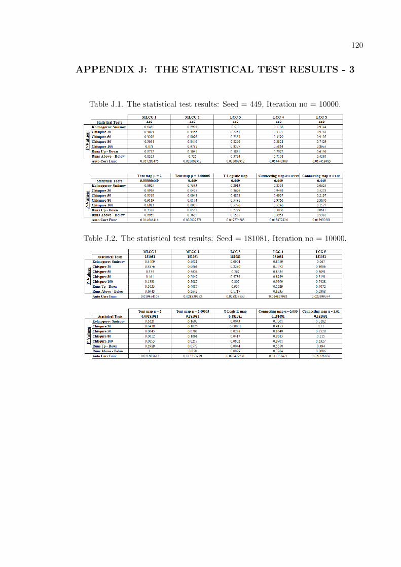
120
APPENDIX J: THE STATISTICAL TEST RESULTS - 3
Table J.1: The statistical test results: Seed = 449, Iteration no = 10000.
Table J.2: The statistical test results: Seed = 181081, Iteration no = 10000.

121
Table J.3: The statistical test results: Seed = 890123, Iteration no = 10000.
Table J.4: The statistical test results: Seed = 1, Iteration no = 10000.

122
Table J.5: The statistical test results: Seed = 9301, Iteration no = 10000.
Table J.6: The statistical test results: Seed = 566231, Iteration no = 10000.

123
Table J.7: The statistical test results: Seed = 27683, Iteration no = 10000.
Table J.8: The statistical test results: Seed = 77, Iteration no = 10000.

124
Table J.9: The statistical test results: Seed = 746011, Iteration no = 10000.

125
APPENDIX K: THE STATISTICAL TEST RESULTS - 4
Table K.1: The statistical test results: Seed = 89, Iteration no = 10000.
Table K.2: The statistical test results: Seed = 590223, Iteration no = 10000.
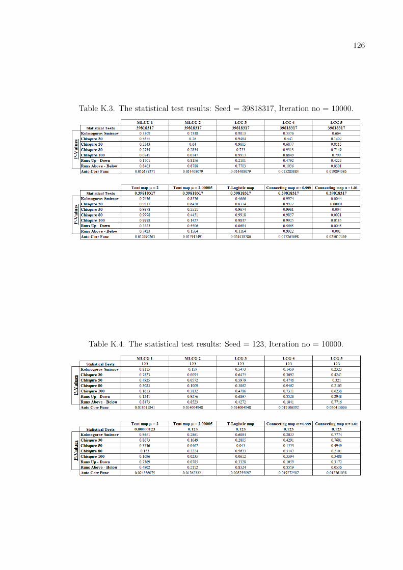
126
Table K.3: The statistical test results: Seed = 39818317, Iteration no = 10000.
Table K.4: The statistical test results: Seed = 123, Iteration no = 10000.

127
Table K.5: The statistical test results: Seed = 6979, Iteration no = 10000.
Table K.6: The statistical test results: Seed = 821129, Iteration no = 10000.

128
Table K.7: The statistical test results: Seed = 915612, Iteration no = 10000.
Table K.8: The statistical test results: Seed = 112319, Iteration no = 10000.

129
Table K.9: The statistical test results: Seed = 277, Iteration no = 10000.
Table K.10: The statistical test results: Seed = 4612967, Iteration no = 10000.

130
APPENDIX L: HISTOGRAMS WITH DIFFERENT
SUBINTERVALS
In this part, we show that the change in the number of subintervals does not
improve to determine the uniformity of the numbers. Three maps are selected to
represent the relations between the histograms of samples for four different numbers
of subintervals: 30, 50, 80, and 100. As seen in Table L.1, the first map passes the
half of the chi-square tests, the second one is successful for all tests, and the last one
is unsuccessful for all tests. Note that p-values of 0.05 is used as the test criteria.
Table L.1: The chi-square test results for MLCG 1, LCG 3, and connecting map
(α = 1.01): Seed = 566231857, Iteration no = 10000.
As can be observed in Figure L.1, Figure L.2, and Figure L.3, there is no relation
between the test results and the histograms of the numbers. The difference between
the histogram of the numbers that are passed chi-square test and the histogram of the
number that are not passed chi-square test cannot be detected easily. So the number
of subinterval is randomly selected as 50 to understand the general behavior of the
numbers for the uniformity test.

131
(a) Histogram with 30 subintervals (b) Histogram with 50 subintervals
(c) Histogram with 80 subintervals (d) Histogram with 100 subintervals
Figure L.1: Histograms for MLCG 1: Seed = 566231857, Iteration no = 10000.

132
(a) Histogram with 30 subintervals (b) Histogram with 50 subintervals
(c) Histogram with 80 subintervals (d) Histogram with 100 subintervals
Figure L.2: Histograms for LCG 3: Seed = 566231857, Iteration no = 10000.

133
(a) Histogram with 30 subintervals (b) Histogram with 50 subintervals
(c) Histogram with 80 subintervals (d) Histogram with 100 subintervals
Figure L.3: Histogram for connecting map (α = 1.01): Seed = 0.566231857, Iteration
no = 10000.

134
REFERENCES
1. Law, A. M. and W.D. Kelton, Simulation Modeling & Analysis, 3rd ed., McGraw-
Hill, New York City, 2000.
2. Banks, J., J.S. Carson, B.L. Nelson, and D.M. Nicol, Discrete-Event System
Simulation, 4th ed., Prentice Hall, NJ, 2005.
3. Knuth D.E., The Art of the Computer Programing Vol. 2: Seminumerical
Algorithms, 2nd ed., Addison Wesley, Boston, 1981.
4. James, F., “A Review of Pseudorandom Number Generators”, Computer Physics
Communications, Vol. 60, Issue 3, pp. 329-344, 1988.
5. Phatak, S.C. and S.S. Rao, “Logistic map: A Possible Random Number Generator”,
Physics Review, Vol. 51, Issue 4, pp. 3670-3678, 1995.
6. Niederreiter, H., “A Statistical Analysis of Generalized Feedback Shift
Register Pseudorandom Number Generators”, SIAM Journal on Scientific and
Statistical Computing, Vol. 8, Issue 6, pp. 1035-1051, 1987.
7. Matsumoto, M. and Y. Kurita, “Twisted GFSR Generators”, ACM Transactions
on Modeling and Computer Simulation, Vol. 2, Issue 3, pp. 179-194, 1992.
8. Matsumoto, M. and Y. Kurita, “Twisted GFSR Generators II”, ACM Transactions
on Modeling and Computer Simulation, Vol. 4, Issue 3, pp. 254-266, 1994.
9. Matsumoto, M. and T. Nishimura, ’Mersenne Twister: A 623-dimensionally
Equidistributed Uniform Pseudorandom Number Generator”, ACM Transactions
on Modeling and Computer Simulation, Vol. 8, Issue 1, pp. 3-30, 1998.
10. L’Ecuyer, P., “Efficient and Portable Combined Random Number Generators”,
.Communication of ACM, Vol. 31, Issue 6, pp. 742-749, 1988.

135
11. L’Ecuyer, P., “Random Numbers for Simulation”, Communication of ACM, Vol. 33,
Issue 10, pp. 85-97, 1990.
12. Gentle, J. E., W. Haerdle, and Y. Mori, The Handbook of Computational Statistics,
2nd ed., Springer-Verlag, Berlin, 2011.
13. Lewis, T. G. and W. H. Payne, “Generalized Feedback Shift Register Pseudorandom
Number Algorithms”, Journal of the ACM, Vol. 20, Issue 3, pp. 456468, 1973.
14. Sobottka, M. and L.P.L. de Oliveira, “Periodicity and Predictability in Chaotic
Systems”, The American Mathematical Monthly, Vol. 113, Issue 5, pp. 415-424,
2006.
15. Devaney, R. L., An Introduction to Chaotic Dynamical Systems, Addison-Wesley,
Redwood City, CA, 1989.
16. Banks, J., V. Dragon and A. Tones, Chaos: A Mathematical Introduction,
Cambridge University Press, Cambridge, 2003.
17. Banks, J., J. Brooks, G. Cairns, G. Davies and P. Stacey, “On Devaney’s Definition
of Chaos”, The American Mathematical Monthly, Vol. 99, Issue 4, pp. 332-334, 1992.
18. Kraft, R. L., “Chaos, Cantor Sets, and Hyperbolicity for the Logistic Maps”,
The American Mathematical Monthly, Vol. 106, Issue 5, pp. 400-408, 1999.
19. Vellkoop, M. and R.Berglund, “On Intervals, Transitivity=Chaos”, The American
Mathematical Monthly, Vol. 101, Issue 4, pp. 353-355, 1994.
20. Alligood, K., T. D. Sauer and J. A. Yorke, Chaos: An Introduction to Dynamical
Systems, Springer-Verlag, New York City, 1996.
21. Ott, E., Chaos in Dynamical Systems, Cambridge University Press, Cambridge,
2002.

![Small Random Perturbations of Dynamical Systems and …ruelle/PUBLICATIONS/[65].pdf · Small Random Perturbations of Dynamical Systems and the Definition of Attractors David Ruelle](https://img.pdfslide.us/doc/110x75/5a9e3b927f8b9aee4a8ba77f/small-random-perturbations-of-dynamical-systems-and-ruellepublications65pdfsmall.jpg)