Random number generation

Algorithms and Transforms to Univariate Distributions

Random number generators

Creating numbers that

• are uniformly distributed on the interval (0,1)

• have low autocorrelation

• are unpredictable

Could that be achieved in practice?

Two basic types of random number generators (RNG):

• Hardware generators, also called True Random Number Generators (TRNG)

– Creates random numbers “physically”

– Physical processes (thermal noise, photo electric effects,…) or Mechanic devices (wheels of fortune, tombola machines, dices,…)

– Satisfy conditions of independence and uniform distribution, but has limitations with respect to the amount of numbers that can be produced.

– See further e.g. http://www.robertnz.net/hwrng.htm

• Software generators, also called Pseudo Random Number

Generators (PRNG) – Create random numbers using a mathematical or cryptographic algorithm

– Classic examples: Congruential generators

– Modern methods: Blum-Blum-Shub generator, Shift-register-methods, Mersenne Twister, Blowfish cipher

– Come as embedded functions in software or can be linked as separate objects to the program code.

– The numbers are not truly random; attention must be made to the type of application.

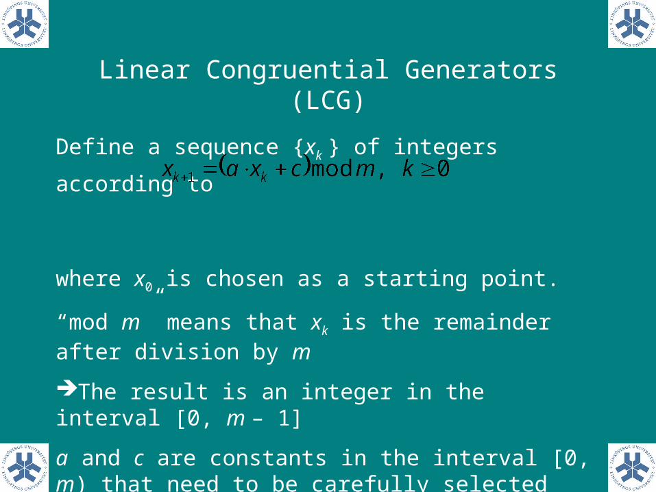
Linear Congruential Generators (LCG)

Define a sequence {xk } of integers according to

where x0 is chosen as a starting point.

“mod m” means that xk is the remainder after division by m

The result is an integer in the interval [0, m – 1]

a and c are constants in the interval [0, m) that need to be carefully selected

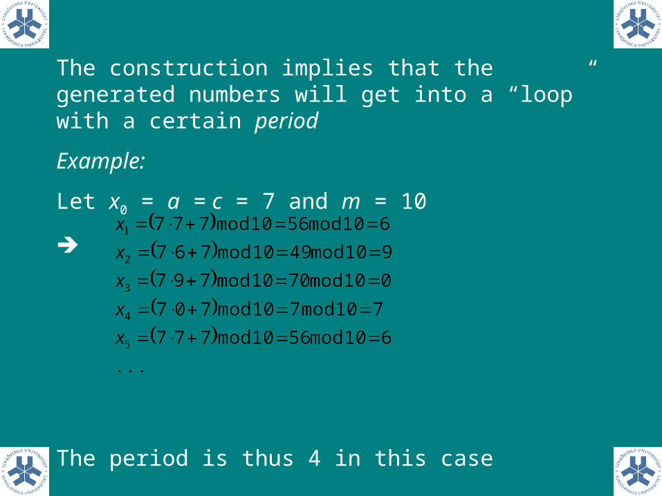
The construction implies that the generated numbers will get into a “loop” with a certain period

Example:

Let x0 = a = c = 7 and m = 10

The period is thus 4 in this case

Clearly, for a generator to be useful, one condition is that the period is long.

How long can it be?

As there are only m possible values, the maximum period length must be m. This is named full period.

Exercise: Consider the case where a = c =1

What are your findings?

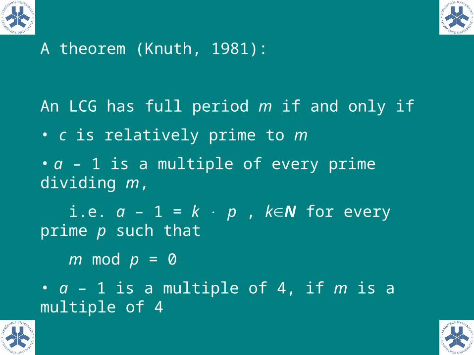
A theorem (Knuth, 1981):

An LCG has full period m if and only if

• c is relatively prime to m

• a – 1 is a multiple of every prime dividing m,

i.e. a – 1 = k p , kN for every prime p such that

m mod p = 0

• a – 1 is a multiple of 4, if m is a multiple of 4

For LCGs to work on a computer, the period cannot be longer than the word size, i.e. 2B, where B is the number of bits.

LCGs are thus constructed so that the full period coincides with the word size.

However, a and c must the be chosen to achieve as much randomness as possible.

Guides for this can be found in several publications; the initial standard reference is

Knuth D. (1981) The Art of Computer Programming. Volume 2 – Seminumerical Algorithms. 2nd ed. Addison-Wesley

Each generated integer is transformed into the interval [0,1) by dividing by m, i.e. uk = xk / m.

Usually, if a zero is obtained, the next value in the sequence is used instead.

The so-obtained sequence of real numbers {uk } are for “good” LCGs uniformly distributed over the interval (0,1).

The starting value x0

• is called the seed to the generator

• has often been set by the computer system clock

• is more and more set by more sophisticated techniques

– to prevent predictability of the sequence

– to ensure unique seeds (if clock frequency is low compared with the process to be run)

• can be used to always create the same sequence of pseudo random numbers if e.g. different scenarios should be compared.

LCGs as well as more modern generators (Mersenne Twister) can create series of random numbers fully acceptable for most

computational statistics studies.

When RNGs are to be used e.g. as components in games (roulette, bingo, lotteries, etc.) both for creating tickets and for drawing winning results, care must be taken in order to prevent the random numbers being predictable.

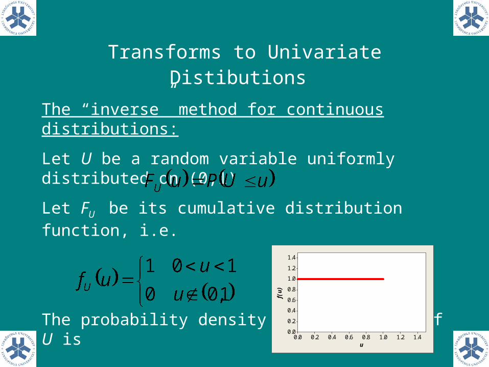
Transforms to Univariate Distibutions

The “inverse” method for continuous distributions:

Let U be a random variable uniformly distributed on (0,1)

Let FU be its cumulative distribution function, i.e.

The probability density function (pdf) of U is

u

f(u)

1.41.21.00.80.60.40.20.0

1.4

1.2

1.0

0.8

0.6

0.4

0.2

0.0

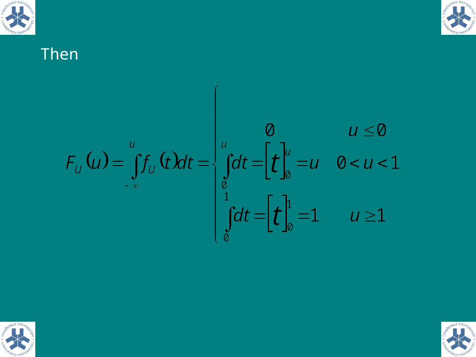
Then

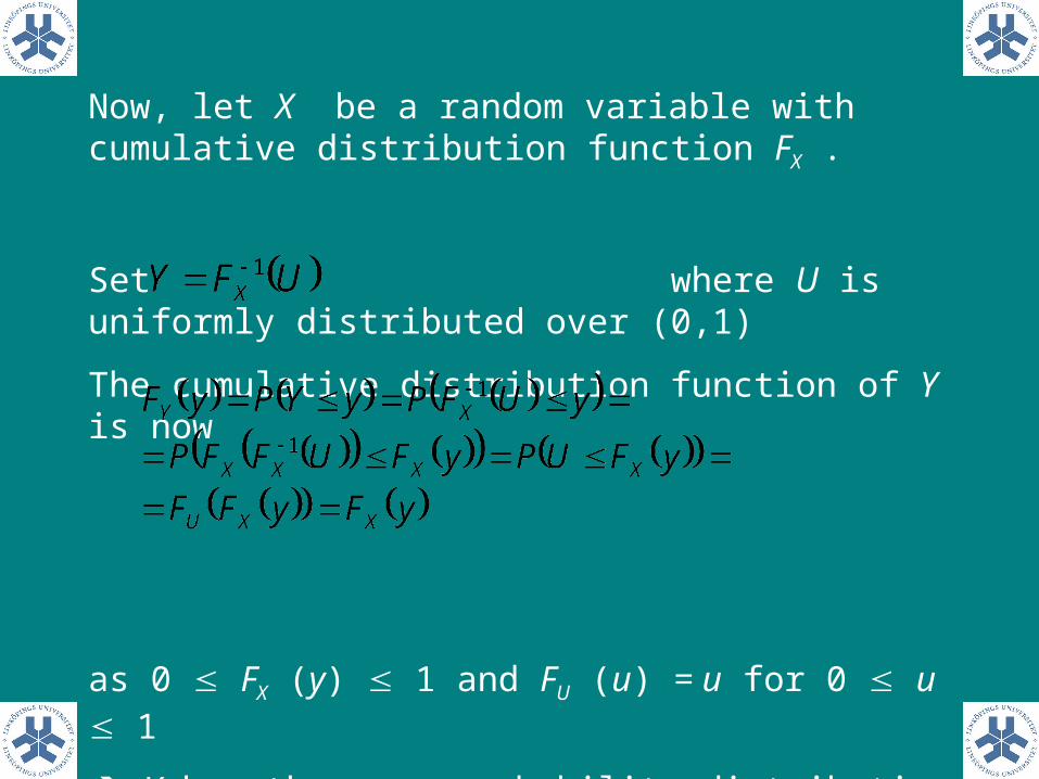
Now, let X be a random variable with cumulative distribution function FX .

Set where U is uniformly distributed over (0,1)

The cumulative distribution function of Y is now

as 0 FX (y) 1 and FU (u) = u for 0 u 1

Y has the same probability distribution as X !!

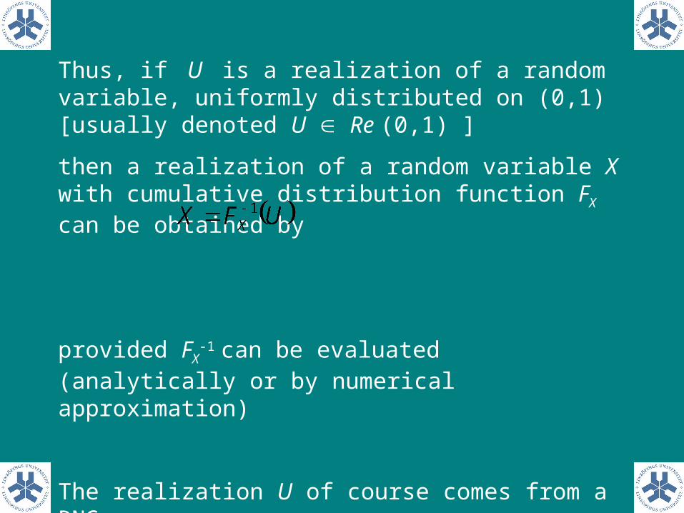
Thus, if U is a realization of a random variable, uniformly distributed on (0,1) [usually denoted U Re (0,1) ]

then a realization of a random variable X with cumulative distribution function FX can be obtained by

provided FX-1 can be evaluated (analytically or by numerical

approximation)

The realization U of course comes from a RNG.

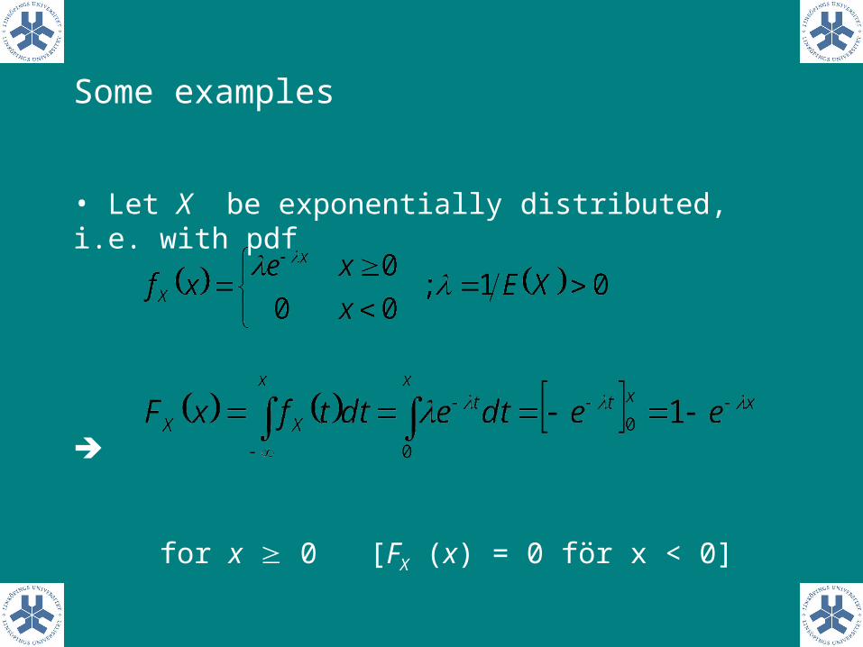
Some examples

• Let X be exponentially distributed, i.e. with pdf

for x 0 [FX (x) = 0 för x < 0]

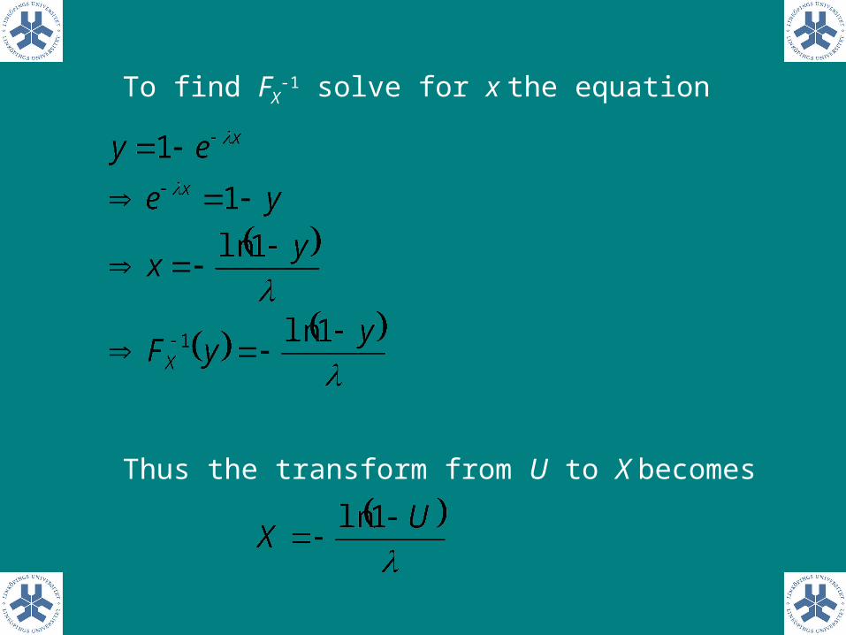
To find FX-1 solve for x the equation

Thus the transform from U to X becomes

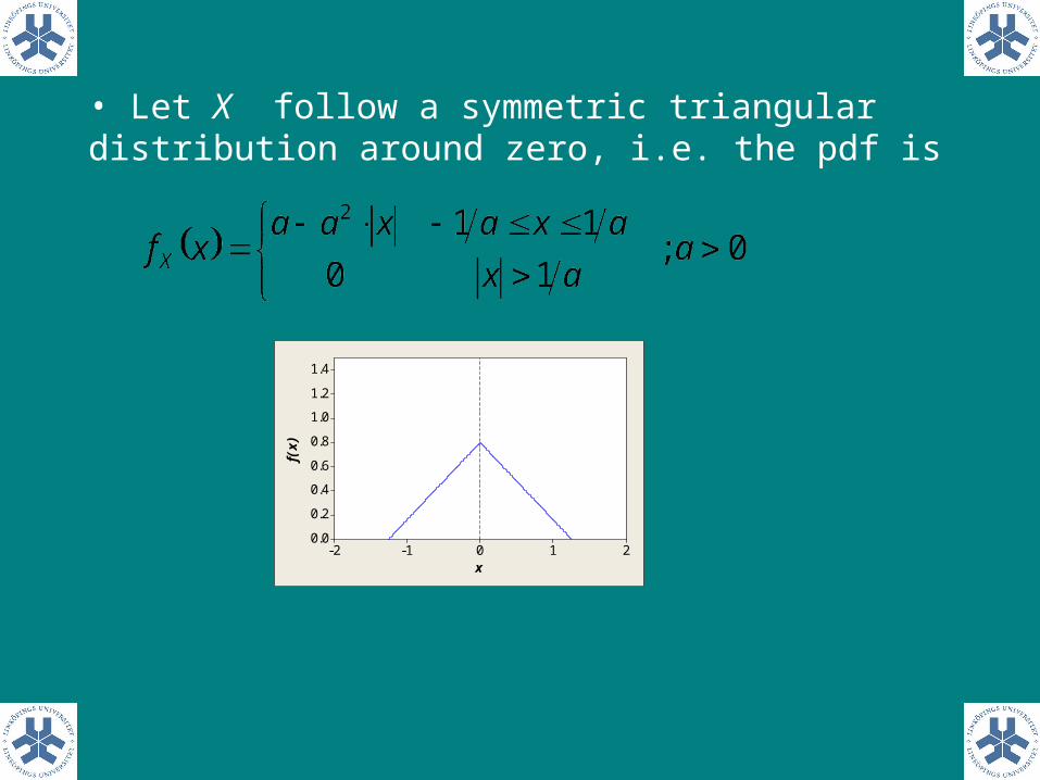
• Let X follow a symmetric triangular distribution around zero, i.e. the pdf is

x

f(x)

210-1-2

1.4

1.2

1.0

0.8

0.6

0.4

0.2

0.0

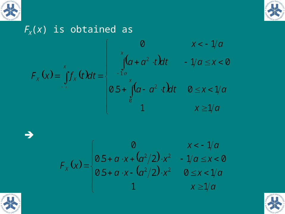
FX(x) is obtained as

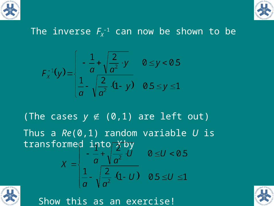
The inverse FX-1 can now be shown to be

(The cases y (0,1) are left out)

Thus a Re(0,1) random variable U is transformed into X by

Show this as an exercise!

Practical considerations with the “inverse” method:

1. When the inverse cumulative distribution can be explicitly derived No problem!

2. When not Numerical solution necessary Usually time-consuming

When is 2 the case?

Unfortunately quite often, and the most obvious example is that of normally distributed random variables (coming soon)

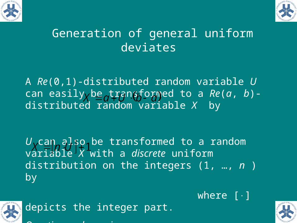
Generation of general uniform deviates

A Re(0,1)-distributed random variable U can easily be transformed to a Re(a, b)-distributed random variable X by

U can also be transformed to a random variable X with a discrete uniform distribution on the integers (1, …, n ) by

where [] depicts the integer part.

Question and exercise:

• Why do we need to add “1”?

• How can U be transformed to a random variable Y with a discrete uniform distribution on the integers (50, 55, 60) ?

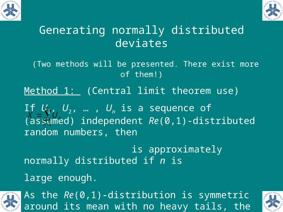
Generating normally distributed deviates

(Two methods will be presented. There exist more of them!)

Method 1: (Central limit theorem use)

If U1, U2, … , Un is a sequence of (assumed) independent Re(0,1)-distributed random numbers, then

is approximately normally distributed if n is

large enough.

As the Re(0,1)-distribution is symmetric around its mean with no heavy tails, the convergence is quite fast.

Exercise:

• What is the mean and standard deviation of X ?

• How can we use X to further transform to any normal distribution?

• Why would n = 12 be a good choice?

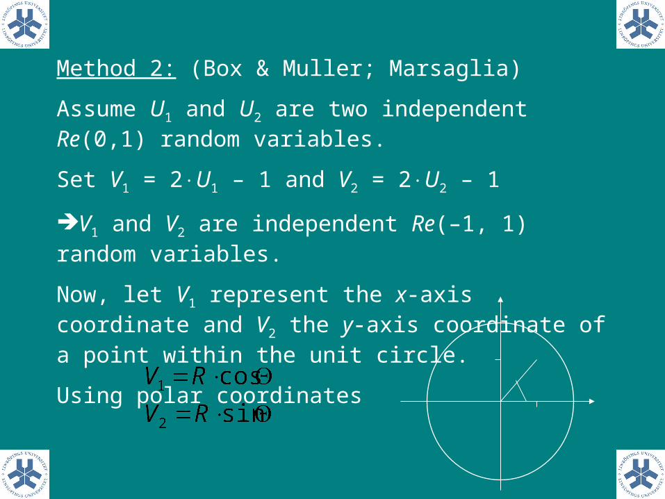
Method 2: (Box & Muller; Marsaglia)

Assume U1 and U2 are two independent Re(0,1) random variables.

Set V1 = 2U1 – 1 and V2 = 2U2 – 1

V1 and V2 are independent Re(–1, 1) random variables.

Now, let V1 represent the x-axis coordinate and V2 the y-axis coordinate of a point within the unit circle.

Using polar coordinates

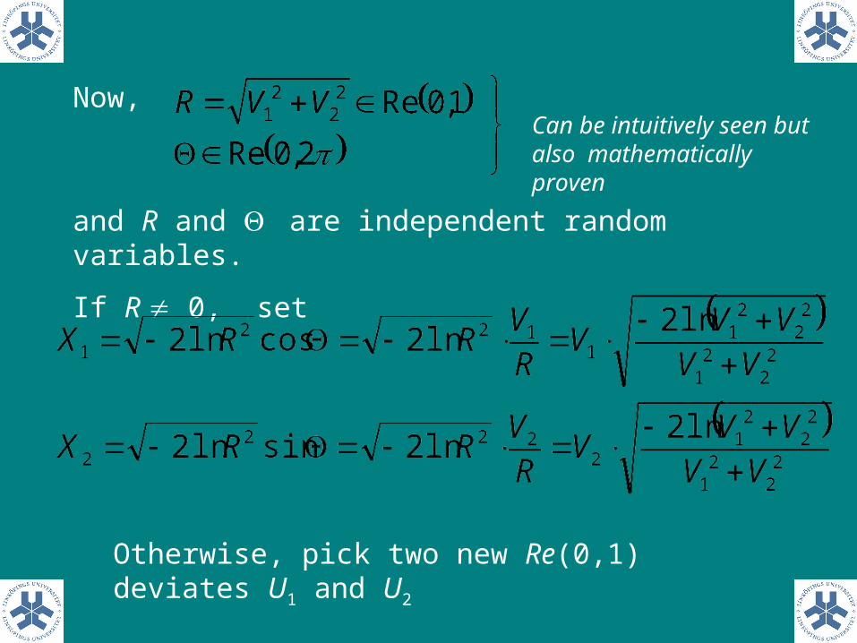
Now,

and R and are independent random variables.

If R 0, set

Can be intuitively seen but also mathematically proven

Otherwise, pick two new Re(0,1) deviates U1 and U2

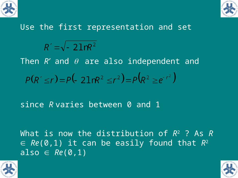
Use the first representation and set

Then R’ and are also independent and

since R varies between 0 and 1

What is now the distribution of R2 ? As R Re(0,1) it can be easily found that R2 also Re(0,1)

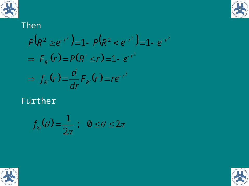
Then

Further

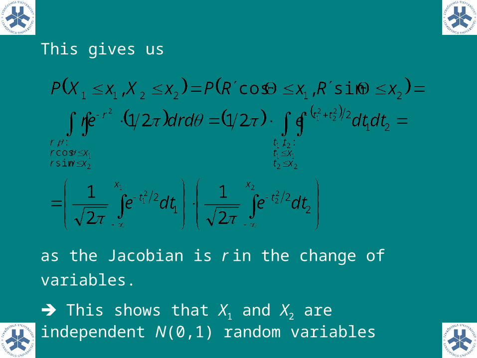
This gives us

as the Jacobian is r in the change of variables.

This shows that X1 and X2 are independent N(0,1) random variables

Generating general discrete distribution random variables

For a random variable X distributed over a finite (and small) set of M numbers, divide the interval (0,1) into M intervals with lengths equal to the individual probabilities of the M possible values.

If U belongs to interval i let X be equal to value i

Special cases

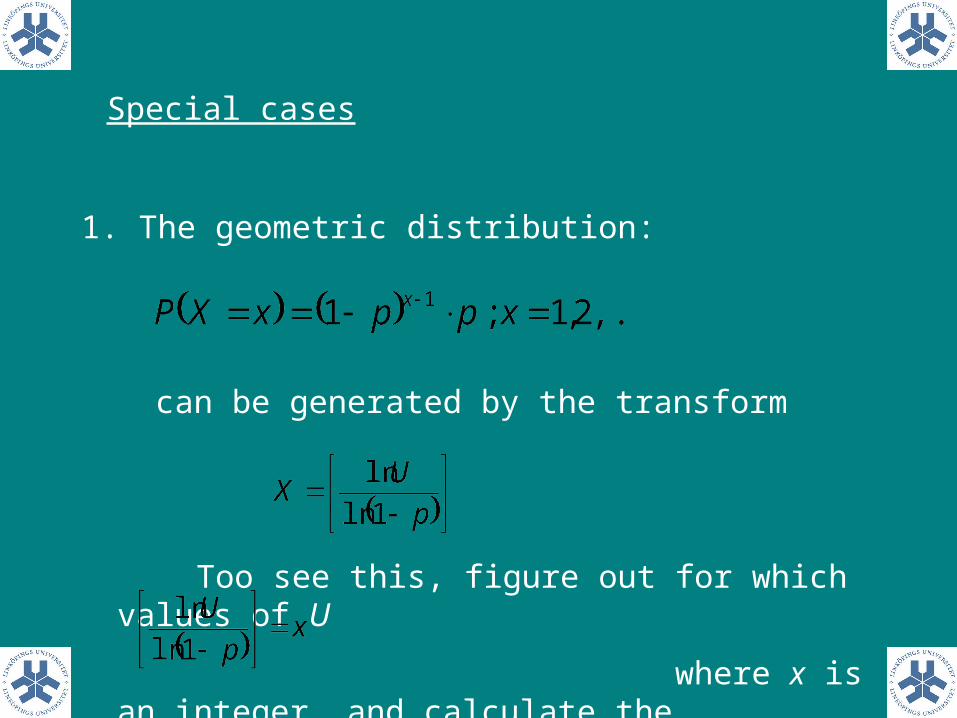
1. The geometric distribution:

can be generated by the transform

Too see this, figure out for which values of U

where x is an integer, and calculate the

corresponding probability

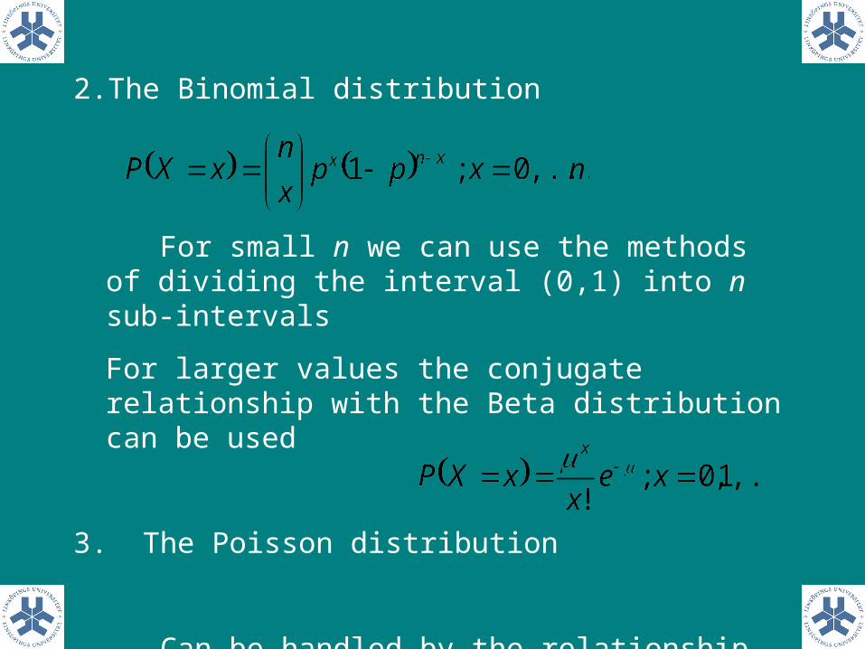
2. The Binomial distribution

For small n we can use the methods of dividing the interval (0,1) into n sub-intervals

For larger values the conjugate relationship with the Beta distribution can be used

3. The Poisson distribution

Can be handled by the relationship with the exponential and gamma distributions