RANDOM MATRIX THEORY - staff.math.su.sestaff.math.su.se/shapiro/UIUC/random_matrices.pdfRANDOM MATRIX THEORY SLAVA KARGIN STATISTICAL LABORATORY, UNIVERSITY OF CAMBRIDGE [email protected]

RANDOM MATRIX THEORY

SLAVA KARGINSTATISTICAL LABORATORY, UNIVERSITY OF CAMBRIDGE

[email protected]

ELENA YUDOVINASTATISTICAL LABORATORY, UNIVERSITY OF CAMBRIDGE

[email protected]

1. Introduction

Random matrix theory is usually taught as a sequence of several graduate courses; wehave 16 lectures, so we will give a very brief introduction.

Some relevant books for the course:

• G. Anderson, A. Guionnet, O. Zeitouni. An introduction to random matrices. [1]• A. Guionnet. Large random matrices: lectures on macroscopic asymptotics.• M. L. Mehta. Random matrices.

The study of random matrices originated in statistics, with the investigation of samplecovariance matrices, and in nuclear physics, with Wigner’s model of atomic nuclei by largerandom matrices.

A random matrix is a matrix with random entries. Let us see what sorts of questions wecan ask about this object and what tools we can use to answer them.

Questions:

Distribution of eigenvalues on the global scale. Typically, thehistogram of eigenvalues looks something like this:

What is the limiting shape of the histogram when the size of the matrix becomes large?

Distribution of eigenvalues at the local scale. The histogram ofspacings between the eigenvalues may look like this:

What is the limiting shape of this histogram?

Is there universality of these shapes with respect to small changes in the distribution ofthe matrix entries?

Are the eigenvectors local-ized?

magnitude

component

magnitude

component

Localized: one large componentDelocalized: no dominant component

Date: Michaelmas 2011.1

2 KARGIN - YUDOVINA

Approaches:

• Method of traces (combinatorial): for a function f , we have∑N

i=1 f(λi) = Tr f(X),and the right-hand side can be studied using combinatorial methods.• Stieltjes transform method: we study the meromorphic function Tr

(1

X−z

), whose

poles are the eigenvalues of X.• Orthogonal polynomials: in some cases, the distribution of eigenvalues can be written

out explicitly and related to orthogonal polynomials, for which there is an extensivetheory.• Stochastic differential equations: if the entries of the random matrix evolve according

to some stochastic process described by an SDE, then the eigenvalues also evolveaccording to an SDE which can be analyzed.• Esoterica: Riemann-Hilbert, free probability, etc.

RANDOM MATRIX THEORY 3

2. Method of Traces: Wigner random matrices

Let X be an N × N symmetric real-valued matrix. The matrix entries Xij are iid real-

valued random variables (for i ≤ j). Let Zij =√NXij. We assume EZij = 0, EZ2

ij = 1,

E |Zij|k = rk <∞ for all k (and all N). (Most of these assumptions can be relaxed.)

Definition. The empirical measure of the eigenvalues is LN = 1N

∑Ni=1 δλi , where λi are

eigenvalues of X.

We will use the following notational convention: for a measure µ on R and a function f ,we write

〈µ, f〉 :=

∫Rf(x)µ(dx).

In particular, 〈LN , f〉 = 1N

∑f(λi).

Definition. The density of states LN is the expected value of the random measure LN .

Note that the expectation is with respect to the randomness in {Xij}.Let σ be the measure on R with density 1

2π

√(4− x2)+ (so the support of σ is confined to

[−2, 2]). The measure σ is often called (Wigner’s) semicircle law.

Theorem 2.1 (Wigner). For any bounded continuous function f ∈ Cb(R),

P(|〈LN , f〉 − 〈σ, f〉| > ε)→ 0 as N →∞

In other words, LN → σ weakly, in probability.

Proof. The proof relies on two lemmas. The first asserts that the moments of LN convergesto the moments of σ; the second asserts that the moments of LN converges to the momentsof LN in probability.

Lemma 2.2. LN → σ in moments, i.e. as N →∞, for any k ≥ 0 we have

〈LN , xk〉 → 〈σ, xk〉 =

{0, k odd1

k2+1

(kk/2

), k even.

(Note that this is a statement about convergence in R.)The even moments of σ coincide with the so-called Catalan numbers, which frequently

arise in various enumeration problems in combinatorics.

Lemma 2.3. As N →∞, for any k we have

P(∣∣〈LN , xk〉 − 〈LN , xk〉∣∣ > ε)→ 0

(It will be sufficient to show that the variance of 〈LN , xk〉 tends to 0.)Altogether, Lemmas 2.2 and 2.3 show that moments of LN converge to moments of sigma

in probability. In a general situation, the convergence of moments does not imply the weakconvergence of measures. However, this is true for a wide class of limiting measures, inparticular for the measures that are uniquely determined by its moments. See, for example,Theorem 2.22 in Van der Vaart’s “Asymptotic Statistics” [23].

For σ, we can give a direct proof. (See the outline of the general argument below.)Supposing Lemmas 2.2 and 2.3 to hold, the proof proceeds as follows:

4 KARGIN - YUDOVINA

Let f ∈ Cb(R) and M := sup |f(x)|. Observe that for every polynomial Q,

P(|〈LN − σ, f〉| > ε) ≤ P(|〈LN − σ,Q〉| > ε/2) + P(|〈LN − σ, f −Q〉| > ε/2)

≤ P(∣∣〈LN − LN , Q〉∣∣ > ε/4) + P(

∣∣〈LN − σ,Q〉∣∣ > ε/4)

+P(|〈LN − σ, f −Q〉| > ε/2).

We claim that for every δ > 0 there exists a polynomial Q and an integer N0 so that the thirdterm is less than δ for all N ≥ N0. Given this polynomial Q, the first two terms converge to0 as N →∞ as a result of Lemmas 2.3 and 2.2 respectively, and this proves the theorem.

To prove that the claim holds, choose (by using the Weierstrass approximation theorem)

Q =∑K

k=0 akxk such that

(1) sup|x|≤5|f(x)−Q(x)| ≤ ε/8.

Let A = max{|ak|}.Note that since σ supported on [-2,2], hence |〈σ, f − Q〉| ≤ ε/8 < ε/4. Therefore, the

claim will follow if for every δ > 0, we show that there exists N0, such that

(2) P{|〈LN , f −Q〉| > ε/4} ≤ δ

for all N > N0.Note that

P{|〈LN , f −Q〉| > ε/4} ≤ P{|〈LN , (f −Q)1|x|>5〉| > ε/8}

≤ P{|〈LN , 1|x|>5〉| >

ε

8M(K + 1)

}+

K∑k=0

P{|〈LN , |x|k1|x|>5〉| >

ε

8A(K + 1)

}.

Let C := 8(K + 1) max{M,A} and observe by the Markov inequality that

Tk := P(〈LN , |x|k 1{|x|>5}〉 > ε/C) ≤ C

εE〈LN , |x|k 1{|x|>5}〉 ≤

C〈LN , x2k〉ε5k

≤ C

ε

(4

5

)k.

for all integer k ≥ 0 and N ≥ N0(k). The last inequality follows by examining the form ofthe moments of σ (to which the moments of LN converge).

Note that Tk is an increasing sequence. For every δ > 0 it is possible to find L ≥ K suchthat

TL ≤δ

K + 1for all N ≥ N0 = N0(L). Then Tk ≤ δ

K+1for all k = 0, . . . , K, which implies that

P{|〈LN , f −Q〉| > ε/4}This completes the proof. � �

Here is the outline of the high-level argument that shows that the convergence of momentsimplies the weak convergence of probability measures provided that the limiting measure isdetermined by its moments. Suppose for example that we want to show that LN convergesto σ weakly.


Since the second moments of LN are uniformly bounded, hence this sequence of measuresis uniformly tight, by Markov’s inequality. By Prohorov’s theorem, each subsequence hasa further subsequence that converges weakly to a limit L. It is possible to show that themoments of L must equal to the limit of the moments of LN (see Example 2.21 in van derVaart). Since σ is uniquely determined by its moments, hence L must equal σ for everychoice of the subsequence. This is equivalent to the statement that LN converges weakly toσ.

We now move on to the proofs of the lemmas:

Proof of Lemma 2.2. Write

〈LN , xk〉 = E

(1

N

N∑i=1

λki

)=

1

NETr (Xk) =

1

N

∑i=(i1,i2,...,ik)

E(Xi1,i2Xi2,i3 . . . Xiki1).

Let Ti = E(Xi1,i2Xi2,i3 . . . Xiki1).To each word i = (i1, i2, . . . , ik) we associate a graph and a path on it. The vertices of

the graph are the distinct indices in i; two vertices are connected by an edge if they areadjacent in i (including ik and i1); and the path simply follows the edges that occur in iconsecutively, finishing with the edge (ik, i1). The important feature is that the expectedvalue of Ti depends only on the (shape of) the associated graph and path, and not on theindividual indices.

Observation. If the path corresponding to i traverses some edge only once, then E(Ti) = 0(since we can take out the expectation of the corresponding term).

Therefore, we are only interested in those graph-path pairs in which every edge is traversedat least twice. In particular, all such graphs will have at most k/2 edges, and (because thegraph is connected) at most k/2 + 1 vertices.

Exercise 1. If the graph associated to i has ≤ k/2 vertices, then E(Ti) ≤ ckE |Xij|k ≤ BkNk/2

for some constants ck, Bk. (Use Holder’s inequality.)

Now, for a fixed graph-path pair with d vertices, the number of words giving rise to it (i.e.the number of ways to assign indices to the vertices) is N(N − 1) . . . (N − d + 1) ≈ Nd. Inaddition, the number of graph-path pairs with ≤ k/2 + 1 vertices and ≤ k/2 edges is somefinite constant depending on k (but not, obviously, on N).

Consequently, by Exercise 1 the total contribution of the words i whose graphs have ≤ k/2vertices to 1

N

∑i E(Ti) is O(N−1Nk/2N−k/2) = O(N−1).

Therefore, we only care about graphs with exactly k/2+1 vertices, hence exactly k/2 edges,each of which is traversed twice. For each such graph, 1

NE(Ti) = 1

NE(X2

ij)k/2 = 1

Nk/2+1 , while

the number of ways to label the vertices of such a graph-path pair is N(N−1) . . . (N− k2−1) ≈

Nk/2+1. We conclude that the kth moment 〈LN , xk〉, for k even, converges to the number ofequivalence classes of pairs G,P where G is a tree with k/2 edges and P is an oriented pathalong G with k edges traversing each edge of G twice. (For k odd it converges to 0.)

Here the equivalence is with respect to a re-labelling of vertices. We now count the numberof these objects.

An oriented tree is a tree (i.e., a graph without closed paths of distinct edges) embeddedin a plane. A rooted tree is a tree that has a special edge (“root”), which is oriented, thatis, this edge has a start and end vertices. Two oriented rooted tree are isomorphic if there

6 KARGIN - YUDOVINA

is a homeomorphism of the corresponding planes which sends one tree to another one insuch a way that the root goes to the root and the orientations of the root and the planeare preserved. Figure 1 shows an example of two trees that are equivalent in the graph-theoretical sense as rooted trees, but not equivalent as oriented rooted trees. (There is noisomorphism of planes that sends the first tree to the second one.)

Figure 1. Two non-isomorphic oriented rooted trees

Figure 2 shows all non-isomorphic oriented rooted trees with 3 edges.

Figure 2. Oriented rooted trees with 3 edges

Claim 2.4. There exists a bijection between equivalence classes of (G,P ) where G is a treewith k/2 edges and P is an oriented path along G with k edges traversing each edge of Gtwice, and non-isomorphic oriented rooted trees.

Proof. Given a path P on G, we embed G into the plane as follows: put the starting vertexat the origin, and draw unit-length edges out of it, clockwise from left to right, in the orderin which they are traversed by P . Continue for each of the other vertices.

Conversely, given an embedding of G with a marked directed edge, we use that edge asthe starting point of the walk P and continue the walk as follows: When leaving a vertex,pick the next available distance-increasing edge in the clockwise direction and traverse it. Ifthere are no available distance-increasing edges, go back along the unique edge that decreasesdistance to the origin. It is easy to see that every edge will be traversed exactly twice. �

We can think of the embedded tree in terms of its thickening – “fat tree” or “ribbongraph”. Then this is actually a rule for the traversal of the boundary of the fat graph in theclockwise direction. Figure 3 shows an example of a fat tree.

Claim 2.5. The oriented rooted trees are in bijection with Dick paths, i.e. paths of a randomwalk Sn on Z such that S0 = Sk = 0 and Sj ≥ 0 for all j = 0, 1, . . . , k.

Proof. Let the embedding have unit-length edges. The random walk Sn is simply measuringthe distance (along the graph) of the nth vertex in the path from the root (the vertex at thesource of the marked edge). If Sn is increasing, we need to create a new edge to the rightof all previously existing ones; if Sn is decreasing, we need to follow the unique edge leadingfrom the current vertex towards the root (“towards” in the sense of graph distance). �


Figure 3. A fat tree

Figure 4. A Dick path and the corresponding oriented rooted tree

An example of this bijection is shown in Figure 4.We now count the number of Dick paths as follows:

#{all paths with S0 = Sk = 0}−#{paths with S0 = Sk = 0 and Sj = −1 for some j ∈ {1, . . . , k − 1}}

The first term is easily seen to be(kk/2

)(we have k jumps up and k jumps down). For the

second term, we argue that such paths are in bijection with paths starting at 0 and endingat −2. Indeed, let j be the last visit of the path to −1, and consider reflecting the portionof the path after j about the line y = −1: it is easy to see that this gives a unique pathterminating at −2 with the same set of visits to −1. The number of paths with S0 = 0 andSk = −2 is easily seen to be

(k

k/2−1

)(we have k− 1 jumps up and k + 1 jumps down), so we

conclude

limN→∞

〈LN , xk〉 =

{0, k odd(kk/2

)−(

kk/2−1

)= 1

k/2+1

(kk/2

), k even

�

Proof of Lemma 2.3. By Chebyshev’s inequality, it suffices to show

Var(〈LN , xk〉)→ 0 as N →∞.We compute

Var(〈LN , xk〉) =1

N2

∑i,j

E(TiTj)− E(Ti)E(Tj) =1

N2

∑i,j

Cov(Ti, Tj).

8 KARGIN - YUDOVINA

We associate a graph G and a pair of paths P1 = P1(i), P2 = P2(j) with the pair i, j: thevertices are the union of the indices in i and j, the edges are the pairs (is, is+1) and (jt, jt+1)(with the convention k + 1 = 1), the first path traverses the edges of i in order, the secondpath traverses the edges of j in order.

Observations:

(1) The graph G may end up disconnected, but the corresponding covariance is 0.(2) In fact, for the covariance to be non-zero, every edge of G mush be traversed at least

twice by the union of P1 and P2. In particular, G has at most k edges, and at mostk + 1 vertices.

(3) The number of labellings of the vertices of an equivalence class (G,P1, P2) with atmost k + 1 vertices is at most Nk+1.

(4) The number of equivalence classes of triples (G,P1, P2) with at most k + 1 verticesand k edges is a finite constant (depending on k, but not on N).

(5) Each Cov(Ti, Tj) is bounded by O(N−k).

We conclude that Var(〈LN , xk〉) = O(N−1)→ 0 as required. �

Exercise 2. Show that in fact Var(〈Ln, xk〉) = O(N−2) by showing that the terms with k+1vertices end up having covariance 0. (This is useful for showing almost sure convergencerather than convergence in probability, because the sequence of variances is summable.)

2.1. Scope of the method of traces. There are various ways in which the above analysiscould be extended:

(1) Technical extensions:

• We assumed that Zij =√NXij has all moments. This is in fact unnecessary: we

could truncate the entries Xij and use the fact that the eigenvalues of a matrixare Lipschitz with respect to the entries. All that is necessary is EZij = 0,EZ2

ij = 1.

• If EZ2ij = σij depends on i and j, then in general there is weak convergence

LN → µ for some limiting measure µ (i.e., the variance of LN tends to 0), but µneed not be the semicircle law.

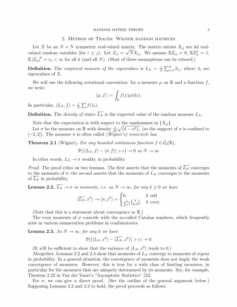
(2) We can also find the laws for some other ensembles:• The Wishart ensemble is XTX where X is an N ×M matrix with iid entries,N → ∞ and M/N → λ. (Moment assumptions as for the Wigner ensemble.)The limit law for the empirical distributions of its eigenvalues is the Marchenko-Pastur law (see example sheet 1), given by

f(x) =1

2πx

√(b− x)(x− a), a = (1−

√λ)2, b = (1 +

√λ)2

plus an atom at 0 if λ < 1 (i.e. if XTX does not have full rank). This law lookslike this:

ba

This is more “useful” than Wigner analysis, because XTX can be thought ofas sample covariances. For example, we can check whether we got something


that looks like noise (in this case eigenvalues of the covariance matrix ought toapproximately follow the Marchenko-Pastur law) or has eigenvalues which areoutliers. For more on this, see N. El Karoui, [17], “Spectrum estimation forlarge dimensional covariance matrices using random matrix theory”, Annals ofStatistics 36:6 (2008), pp. 2757-2790.

(3) Behaviour of the largest eigenvalue: consider 1NETr (XkN

N ), where the moment kNdepends on N . If kN → ∞ as N → ∞, this is dominated by 1

NλkNmax. The difficulty

with the analysis comes from the fact that if kN → ∞ quickly, then more graphshave nonnegligible contributions, and the combinatorics becomes rather nasty. E.g.,Furedi-Komlos [10] showed that (in particular) P(λmax > 2 + δ)→ 0 as N →∞. (Infact, they showed this with some negative power of N in the place of δ.) Soshnikov(in [19] and [20]) has extended this analysis to determine the asymptotic distributionof the largest eigenvalue of the Wigner ensemble.

However, the trace method has various limitations, in particular:

(1) Difficult to say anything about the local behaviour of the eigenvalues (e.g., theirspacings) away from the edge of the distribution (“in the bulk”), because eigenvaluesin the bulk aren’t separated by moments;

(2) Difficult to get the speed of convergence, and(3) Says nothing about the distribution of eigenvectors.

10 KARGIN - YUDOVINA

3. Stieltjes transform method

3.1. Stieltjes transform.

Definition. Suppose µ is a nonnegative finite measure on R. The Stieltjes transform of µ is

gµ(z) =

∫R

1

x− zµ(dx), z ∈ C \ R.

If all the moments of µ are finite (and the resulting series converges), we can rewrite thisas

gµ(z) =

∫R−1

z

1

1− x/zµ(dx) = −1

z

∞∑k=0

mk

zk,

where mk =∫xkµ(dx) is the kth moment of µ.

If µ = LN , then

gLN (z) =1

N

N∑i=1

1

λi − z=

1

NTr

1

XN − zI,

where (XN − z)−1 is the resolvent of XN , for which many relations are known.The important thing about the Stieltjes transform is that it can be inverted.

Definition. A measure µ on R is called a sub-probability measure if µ(R) ≤ 1.

Theorem 3.1. Let µ be a sub-probability measure. Consider an interval [a, b] such thatµ{a} = µ{b} = 0. Then

µ[a, b] = limη→0

∫ b

a

1

πIm gµ(x+ iη)dx

Proof. First, we massage the expression:∫ b

a

1

πIm gµ(x+ iη)dx =

∫ b

a

1

π

∫ ∞−∞

η

(λ− x)2 + η2µ(dλ)dx =∫ ∞

−∞

1

π

(tan−1

(b− λη

)− tan−1

(a− λη

))µ(dλ).

(Note: tan−1 is the inverse tangent function.)Let

R(λ) =1

π

[tan−1

(b− λη

)− tan−1

(a− λη

)];

a plot of this function looks as follows:

1

λ

R(λ)

a b

Some facts:

(1) 0 ≤ R(λ) ≤ 1


(2) tan−1(x)− tan−1(y) = tan−1(x−y1+xy

)and therefore

R(λ) =1

πtan−1

(η(b− a)

η2 + (b− λ)(a− λ)

).

(3) tan−1(x) ≤ x for x ≥ 0.

Let δ be such that µ[a− δ, a+ δ] ≤ ε/5 and µ[b− δ, b+ δ] ≤ ε/5. Now,∣∣∣∣∫R

1[a,b](λ)µ(dλ)−∫RR(λ)µ(dλ)

∣∣∣∣ ≤2ε

5+

∫ a−δ

−∞R(λ)µ(dλ) +

∫ ∞b+δ

R(λ)µ(dλ) +

∫ b−δ

a+δ

(1−R(λ))µ(dλ).

For the first term, if λ < a, b then the argument of the arctangent in R(λ) is positive, so weapply the third fact to get∫ a−δ

−∞R(λ)µ(dλ) ≤ 1

πη

∫ a−δ

−∞

b− aη2 + (b− λ)(a− λ)

µ(dλ).

(Similarly for the second term, where λ > a, b.) It’s not hard to check that the integral isfinite, and bounded uniformly in all small η. Hence the first two terms are ≤ ε

5for sufficiently

small η.Finally, for the third term, we have∫ b−δ

a+δ

(1− 1

πtan−1

(b− λη

)+

1

πtan−1

(a− λη

))µ(dλ) ≤∫ b−δ

a+δ

(1− 2

πtan−1

(δ

η

))µ(dλ)

Now, as η → 0+ we have tan−1(δ/η) → π2

(from below), and in particular the integral willbe ≤ ε

5for all sufficiently small η.

Adding together the bounds gives ≤ ε for all sufficiently small η, as required. �

A somewhat shorter version of the proof can be obtained by observing that as η → 0,R(λ) → 1 for λ ∈ (a, b), R(λ) → 0 for λ ∈ [a, b]c, and R(λ) → 1/2 for λ ∈ {a, b}. Inaddition, R(λ) can be majorized uniformly in η by a positive integrable function. Thisis because R(λ) is uniformly bounded and its tails are ∼ η/λ2. Hence, we can apply thedominated convergence theorem (e.g., property (viii) on p. 44 in [4]) and obtain

(3)1

π

∫RR(λ)µ(dλ)→ µ[a, b].

Corollary 3.2. If two subprobability measures µ, ν have gµ = gν, then µ = ν.

Theorem 3.3. Let {µn} be a sequence of probability measures, with Stieltjes transformsgµn(z). Suppose there is a probability measure µ with Stieltjes transform gµ(z), such thatgµn(z) → gµ(z) holds at every z ∈ A, where A ⊆ C is a set with at least one accumulationpoint. Then µn → µ weakly.

It’s reasonably clear that if µn converges weakly, then the limit must be µ; the main issueis showing that it converges.


Proof.

Definition. We say that a sequence of sub-probability measures µn converges to a sub-probability measure µ vaguely if for all f ∈ C0(R) we have∫

Rfµn(dx)→

∫Rfµ(dx)

Here, the space C0 consists of continuous functions f with f(x)→ 0 as |x| → ∞.Recall that weak convergence is the same statement for all continuous bounded functions

f .Fact: a sequence of sub-probability measures {µn} always has a limit point with respect

to vague convergence (Theorem 4.3.3 on p. 88 in [4]).

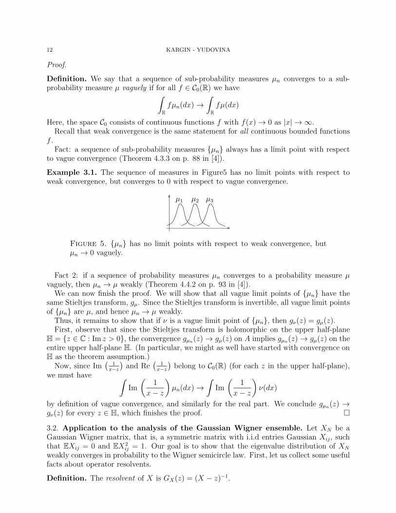
Example 3.1. The sequence of measures in Figure5 has no limit points with respect toweak convergence, but converges to 0 with respect to vague convergence.

µ2µ1 µ3

Figure 5. {µn} has no limit points with respect to weak convergence, butµn → 0 vaguely.

Fact 2: if a sequence of probability measures µn converges to a probability measure µvaguely, then µn → µ weakly (Theorem 4.4.2 on p. 93 in [4]).

We can now finish the proof. We will show that all vague limit points of {µn} have thesame Stieltjes transform, gµ. Since the Stieltjes transform is invertible, all vague limit pointsof {µn} are µ, and hence µn → µ weakly.

Thus, it remains to show that if ν is a vague limit point of {µn}, then gν(z) = gµ(z).First, observe that since the Stieltjes transform is holomorphic on the upper half-plane

H = {z ∈ C : Im z > 0}, the convergence gµn(z)→ gµ(z) on A implies gµn(z)→ gµ(z) on theentire upper half-plane H. (In particular, we might as well have started with convergence onH as the theorem assumption.)

Now, since Im(

1x−z

)and Re

(1

x−z

)belong to C0(R) (for each z in the upper half-plane),

we must have ∫Im

(1

x− z

)µn(dx)→

∫Im

(1

x− z

)ν(dx)

by definition of vague convergence, and similarly for the real part. We conclude gµn(z) →gν(z) for every z ∈ H, which finishes the proof. �

3.2. Application to the analysis of the Gaussian Wigner ensemble. Let XN be aGaussian Wigner matrix, that is, a symmetric matrix with i.i.d entries Gaussian Xij, suchthat EXij = 0 and EX2

ij = 1. Our goal is to show that the eigenvalue distribution of XN

weakly converges in probability to the Wigner semicircle law. First, let us collect some usefulfacts about operator resolvents.

Definition. The resolvent of X is GX(z) = (X − z)−1.


The Stieltjes transform of LN is

gLN (z) =1

N

N∑i=1

1

λi − z=

1

NTrGXN (z)

and in particular,

EgLN (z) = gLN (z) =1

NETr (GXN (z))

Lemma 3.4 (Resolvent identity).

GX+A(z)−GX(z) = −GX+A(z)AGx(z)

Proof. Multiply by X − z on the right, and by X + A− z on the left. �

Corollary 3.5. Taking A = −X, we get

−1

z−GX(z) =

1

zXGX(z)

so

GX(z) = −1

z+

1

zXGX(z)

Note: Here 1/z is a shortcut for (1/z)IN , where IN is the N ×N identity matrix.

Corollary 3.6.∂Guv

∂Xij

= −GuiGjv −GujGiv

(The question of what A you need to get this is left as an exercise to the reader, but ata guess A should have 0 everywhere except the ijth – and possibly jith – entry, in which itshould have an ε.)

Lemma 3.7. If ξ ∼ N (0, σ2) and f is a differentiable function which grows no faster thana polynomial, then Eξf(ξ) = σ2E(f ′(ξ)).

We now continue the analysis of the Wigner ensemble:

1

NETr (GXN (z)) = −1

z+

1

NzETr (XGX)

= −1

z+

1

Nz

∑i,j

E(XijGji)

= −1

z+

1

N2z

∑i,j

E(∂Gji

∂Xij

)= −1

z+

1

N2z

∑i,j

E(−GjiGij −GjjGii)

= −1

z− 1

N2zE(Tr (G2))− 1

zE((

1

NTrG)2).

Here, the third line follows from Lemma 3.7, and the fourth line follows from Corollary 3.6.Note that 1

N2zTr (G2) = 1

Nz1N

∑Ni=1

1(λi−z)2 , and every term in the sum is bounded by 1

η2,

where η = Im z. In particular, as N →∞, this term → 0.


We conclude

Eg(z) = −1

z− 1

zE(g(z)2) + EN ,

where the error term EN satisfies EN → 0 as N →∞.Now, if we had Varg(z)→ 0 as N →∞, we could write

Eg(z) = −1

z− 1

zE(g(z))2 + EN ,

for some other error term EN → 0 as N →∞. After some technical work, it can be shownthat the solution of this equation converges to the solution of

s(z) = −1

z− 1

zs(z)2

for every z ∈ H, as N → ∞. Since this is the Stieltjes transform of the semi-circle law, byusing Theorem 3.3 we conclude that ELN converges weakly to the semicircle law.

In addition, if Varg(z)→ 0 as N →∞, then g(z)−Eg(z)→ 0 in probability, which allowsus to conclude that LN − LN → 0 weakly in probability.

Hence, all that remains to show is that

Var(g(z)) = Var

(1

N

N∑i=1

1

λi − z

)→ 0.

We have here a sum of many random terms. The problem is that the λi are not at allindependent. One way to handle this problem is to use concentration inequalities.

3.3. Concentration inequalities; LSI.

Definition. Let µ be a measure on Rm. Define W 1,2(µ) as the space of differentiable func-tions f such that f ∈ L2(µ) and ‖∇f‖2 ∈ L2(µ).

Definition. A probability measure µ on Rm is called LSI with constant c if for every f ∈W 1,2(µ) we have ∫

Rmf 2 log

(f 2∫f 2dµ

)dµ ≤ 2c

∫Rm‖∇f‖22dµ.

The name “LSI” here stands for “logarithmic Sobolev inequality”.We compare this with the Poincare inequality:

Varf ≤ c

∫‖∇f‖22dµ.

We have the following facts:

(1) Gaussian measure on R is LSI.(2) If the law of random variable X is LSI with constant c, then the law of αX is LSI

with constant α2c.(3) If µ is LSI with constant c, then the product measure µ⊗µ⊗ . . .⊗µ is LSI with the

same constant c.(4) There is a Bobkov-Gotze criterion for distributions with a density to satisfy LSI with

some finite constant c (see [3]). One useful case is when the density has the formconst × exp(−g(x)), with twice differentiable g(x) and c1 ≤ g′′(x) ≤ c2 for somepositive constants c1, c2.


(5) A discrete measure is not LSI under this definition. However, there is also a discreteversion of LSI, which is satisfied e.g. by the Bernoulli distribution. See example sheet2.

(6) There is a large literature about logarithmic Sobolev inequalities which are usefulin the study of Markov processes. See review by Gross ([12]) or lecture notes byGuionnet and Zegarlinski (http://mathaa.epfl.ch/prst/mourrat/ihpin.pdf) The topicis important and recently found applications in random matrix theory through thestudy of eigenvalues of matrices whose entries follow the Ornstein-Uhlebeck process.However, we are not concerned with these issues in our lectures.

For us, XN has a law which is a product of Gaussian measures with variance 1/N , andhence by Facts 2 and 3, this law is LSI with constant c/N , where c is the LSI constant of thestandard Gaussian measure. The main idea is that the probability of a large deviation of aLipschitz function F (x1, . . . , xn) from its mean can be efficiently estimated if the probabilitydistribution of x1, . . . , xn is LSI.

Definition. A function f : Rm → R is Lipschitz with constant L if

(4) supx 6=y

|f(x)− f(y)|‖x− y‖

≤ L.

Lemma 3.8 (Herbst). Suppose µ is a measure on Rm which is LSI with constant c, andF : Rm → R is Lipschitz with constant L. Then

(1) E[eλ(F−EF )] ≤ ecλ2L2/2, for all λ

(2) P(|F − EF | > δ) ≤ 2 exp(− δ2

2cL2 )(3) VarF ≤ 4cL2.

We will prove this lemma a bit later. In order to apply this lemma we need to find outwhat is the Lipschitz constant of the Stieltjes transform.

Lemma 3.9 (Hoffman-Wielandt inequality). If A and B are symmetric N × N matriceswith eigenvalues

λA1 ≤ λA2 ≤ . . . ≤ λAN , λB1 ≤ λB2 ≤ . . . ≤ λBNthen

N∑i=1

(λAi − λBi )2 ≤ Tr(A−B)2 ≤ 2∑

1≤i≤j≤N

(Aij −Bij)2.

The proof can be found in [1].

Corollary 3.10. The eigenvalues of a matrix X are Lipschitz functions of the matrix entriesXij, with constant

√2.

Corollary 3.11. g(X) = 1N

∑Ni=1

1λi−z is Lipschitz (as a function of X!) with constant

c/√N , where c > 0 depends only on Im z.

(See problem 7 in example sheet 2.)We now use these results to finish the proof of the Wigner law for Gaussian Wigner

matrices: recall we still needed to show that VargN(z)→ 0. We know that the joint measureof the entries of XN is LSI with constant c/N , and gN(z) is Lipschitz (in X) with constant

L = L(η)/sqrt(N), where η = Im z. By applying the Herbst lemma, VargN(z) ≤ 2cL2(η)N2 → 0

for all z ∈ H as N →∞.


Remark. Note that this means that Var∑N

i=11

λi−z → C as N → ∞. (This is surprising,

since usually we would normalize a sum of N random terms by 1/√N . No normalization is

needed at all in this case!)

Proof of Herbst Lemma 3.8. Let A(λ) = logE exp(2λ(F − EF )); we want to show A(λ) ≤2cλ2L.

Applying LSI to f = exp(λ(F − EF )), we have∫e2λ(F−EF ) log

e2λ(F−EF )

eA(λ)dµ ≤ 2c

∫λ2e2λ(F−EF )‖∇F‖22dµ

On the left-hand side, we have∫2λ(F − EF )e2λ(F−EF )dµ− A(λ)

∫e2λ(F−EF )dµ

Note that the first term is λ ∂∂λ

(e2λ(F−EF )); interchanging integration and differentiation, weconclude that the left-hand side is

λ(eA(λ))′ − A(λ)eA(λ) = eA(λ) (λA′(λ)− A(λ)) = eA(λ)λ2(A(λ)

λ

)′(where ′ designates differentiation with respect to λ).

The right-hand side is bounded by 2cλ2eA(λ)L2, since ‖∇f‖22 ≤ L2.Consequently, (

A(λ)

λ

)′≤ 2cL2.

It’s not hard to check by Taylor-expanding that A(λ) = O(λ2), so A(λ)/λ → 0 as λ → 0.Consequently,

A(λ) ≤ 2cL2λ2

as required. Two other statements easily follow from the first one (see exercise sheet 2). �

3.4. Wigner’s theorem for non-Gaussian Wigner matrices by the Stieltjes trans-form method. Recall the definition of the Wigner matrix. Matrix XN be an N × Nsymmetric real-valued matrix with matrix entries Xij. We assume that Zij =

√NXij are

iid real-valued random variables (for i ≤ j) which are taken from a probability distribution,the same one for every N .

We are going to prove the following result by the Stieltjes transform method.

Theorem 3.12 (Wigner). Let XN be a sequence of Wigner matrices, such that EZij = 0,EZ2

ij = 1 and the measure of Zij is LSI, and let LN be its empirical measure of eigenvalues.Then, for any bounded continuous function f ∈ Cb(R),

P(|〈LN , f〉 − 〈σ, f〉| > ε)→ 0 as N →∞

Remark. The assumption that the measure of Zij is LSI can be omitted and the Theoremstill remains valid. The proof of this is somewhat more involved. See Remark at the end ofthe proof and example sheet 2.

Proof: The general idea of the proof is the same as for Gaussian Wigner matrices. Twothings that need to be proved is that

EgN(z) = −1

z− 1

zE(gN(z))2 + EN ,


for some error term EN → 0 as N →∞, and that VargN(z)→ 0. The second claim followsimmediately from the assumption that the measure of Zij is LSI. (Our proof of this resultin the previous section does not depend on the assumption that the entries are Gaussian.)

The proof of the first claim uses some matrix identities.

Lemma 3.13. Let X be a square block matrix

(A BC D

), where A is square and invertible.

ThendetX = detA det(D − CA−1B).

Proof. Carry out the (block) UL decomposition:(A BC D

)=

(A 0C D − C−1AB

)(I A−1B0 I

).

�

Let xi denote the ith column of X without the ith entry. Let X(i) denote the matrix Xwithout the ith row and column.

Lemma 3.14. ((X − z)−1

)ii

=(Xii − z − xTi (X(i) − z)xi

)−1.

Proof. Apply Cramer’s rule:

((X − z)−1)ii =det(X(i) − z)

det(X − z)

Now use Lemma 1 with A = X(i) − z, D = Xii − z (note that the lemma is only directlyapplicable if i = n, but that’s a trivial reordering of the basis). �

Hence,

gN(z) =1

N

∑i

((X − z)−1)ii =1

N

∑i

1

Xii − z − xTi (X(i) − z)−1xi.

We want to get rid of the Xii in the above expression; this is done by the following

Lemma 3.15. Let XN by a sequence of symmetric matrices with independent entries s.t.EXij = 0 and E(

√NXij) = 1. Let XN be defined by setting Xij = 0 if i = j and Xij

otherwise. Then∣∣gXN (z)− gXN (z)

∣∣→ 0 in probability, for all z, as N →∞.

It is also useful to be able to assume that the entries of the random matrix are bounded.For this we have the following tool.

Lemma 3.16. Let XN be a symmetric random matrix, such that Yij =√NXij are i.i.d. for

i ≤ j and all N . Suppose EYij = 0 and EY 2ij = 1. Let

Xij = Xij1√N |Xij |<C − E(Xij1√N |Xij |<C).

Then for every ε > 0, there exists C that depends on ε, z, and the law of Yij only, such that

P{∣∣∣gXN (z)− gXN (z)

∣∣∣ > ε} < ε.

These results are essentially corollaries of the Hoffman-Wielandt inequality, Lemma 3.9.Here is the proof of the result about truncation.


Proof. Clearly, it is enough to show that E∣∣∣gXN (z)− gXN (z)

∣∣∣2 can be made arbitrarily small

uniformly in N. By using the Hoffman-Wielandt inequality, we need to show that

1

NETr

(XN − XN

)2=

1

N2

N∑i,j=1

E(√

NXij −√NXij

)2= E

(√NX12 −

√NX12

)2can be made arbitrarily small uniformly in N . However,

E(√

NX12 −√NX12

)2≤ 2

{[E(Y121Y12<C)]2 + E(Y121Y12>C)2

}.

Since EY12 = 0 and EY 212 = 1, for every ε > 0, we can choose C so large that [E(Y121Y12<C)]2 <

ε and E(Y121Y12>C)2 < ε, which completes the proof. �

In light of these results, we will assume that Xii = 0, i.e.

(5) gN(z) =1

N

∑i

1

−z − xTi (X(i) − z)−1xi.

In addition, we can and will assume that |Xij| < C.We would like to show (and this is the crux of the proof) that the right-hand side of (5)

approaches 1−z−gN (z)

in probability, where gN(z) = EgN(z).

Write it as1

N

∑((−z − gN(z)) + (gN(z)− xTi (X(i) − z)−1xi))

−1

and note that, by the definition of the Stieltjes transform, the quantity −z − gN(z) hasnonzero imaginary part for all z ∈ C \ R.

It suffices to prove that

P(∣∣gN(z)− xTi (X(i) − z)xi)

∣∣ > ε) < c1 exp(−c2Nα)

for some c1, c2, α > 0. Recall that gN(z) = 1N

Tr ((X − z)−1). This is a consequence of thefollowing two claims.

Claim 3.17. With high probability (at least 1− exp(−cNα) for some c, α > 0) we have

(6) P{∣∣∣∣xTi (X(i) − z)−1xi −

1

NTr (X(i) − z)−1

∣∣∣∣ > ε} < c1 exp(−c2(ε)Nα).

Here the expectation is conditional on the realization of X(i).

Claim 3.18. With probability 1,

(7)1

N

∣∣Tr (X(i) − z)−1 − Tr (X − z)−1∣∣ < c(z)

N.

Proof of claim 3.17. Let B = (X(i) − z)−1, a = xi, and note that a and B are independent.Then

E[aTBa|B] = E[∑

aiBijaj|B] =∑i

BiiEa2i =1

N

∑Bii =

1

NTrB.

Next, we use concentration inequalities. The distribution of√NXij is LSI. (It remains LSI

even after truncation.) In addition the norm of the gradient of the quadratic form is bounded


since the random variables Xij are bounded. Hence, the Herbst lemma is applicable and theconclusion follows. �

Remark. The proof of this lemma can be done without invoking LSI, because this is aquadratic form and there are various techniques available for it (vaguely similar to thecentral limit theorems for sums of independent random variables). See example sheet 2.

Proof of claim 3.18. The proof can be done using interlacing inequalities : if λ1 ≤ . . . ≤ λNare eigenvalues of XN , and µ1 ≤ . . . ≤ µN−1 are eigenvalues of X

(i)N , then

λ1 ≤ µ1 ≤ λ2 ≤ . . . ≤ µN−1 ≤ λN .

�


4. Gaussian ensembles

Let ξij, ηij be iid ∼ N (0, 1) (i.e. iid standard normals). Let X be an N ×N matrix.

Definition. X is called the Gaussian Unitary Ensemble (β = 2) if it is complex-valued,hermitian (Xij = Xji), and the entries satisfy

Xij =

{ξii, i = j1√2(ξij +

√−1ηij), i < j

Definition. X is called the Gaussian Orthogonal Ensemble (β = 1) if it is symmetric andreal-valued (Xij = Xji), and has

X − ij =

{√2ξii, i = j

ξij, i < j

There is also a Gaussian Symplectic Ensemble (β = 4) defined using quaternions, or using2N × 2N block matrices over C.

Let us compute the joint distribution of the GUE:

P(X ∈ dx) =

cN exp

(−1

2

∑i

x2ii −1

2

∑i<j

(Rexij)2 + (Imxij)

2

)∏i

dxii∏i<j

dRexijdImxij

= c(2)N exp(−1

2Tr (X2))

∏i

dxii∏i<j

dRexijdImxij.

We will refer to the volume element d(N,2)x.The main observation is that this is invariant under unitary transformations, because trace

is. That is,

P(UXU∗ ∈ dx) = c(2)N exp(−1

2Tr (UXU∗)2)d′(N,2)x

= c(2)N exp(−1

2TrX2)d(N,2)x = P(X ∈ dx),

where d′(N,2)x is induced by the transformation X → UXU∗ from d(N,2)x and we used thefact that d′(N,2)x = d(N,2)x. (See proof of this claim in Section 5.2 of Deift’s book [7].)

For the orthogonal ensemble (β = 1), we get

P(X ∈ dx) = c(1)N exp(−1

4TrX2)d(N,1)x,

where d(N,1)x =∏

i≤j dxij. For the symplectic ensemble (β = 4), we get

P(X ∈ dx) = c(4)N exp(−TrX2)d(N,4)x,

Of course, the orthogonal, resp. symplectic, ensemble has distribution invariant to orthogo-nal, resp. symplectic transformations.

The reason we care about these ensembles is that for them we can compute the exact(non-asymptotic) distributions of eigenvalues.


Theorem 4.1. Suppose XN ∈ Hβ for β = 1, 2, 4. Then the distribution of the eigenvaluesof XN is given by

pN(x1, . . . , xN) = c(β)N

∏i<j

|xi − xj|β exp(−β4

∑x2i )∏

dxi

where the constants c(β)N are normalization constants and can in theory be computed explicitly.

The proof will proceed by changing our basis from the matrix entries to the set of eigen-values and eigenvectors, and then integrating out the component corresponding to the eigen-vectors.

Proof. Write the (Hermitian) matrix X as X = UΛU∗, where Λ is diagonal and U is unitary;the columns of U are the eigenvectors of X. When the eigenvalues of X are are all distinct,this decomposition is unique up to (a) permuting the eigenvalues, and (b) multiplying U bya diagonal matrix with entries eiθ1 , eiθ2 , . . . , eiθN .

Formally, let F : U(N) × RN → H(N) be given by F (U,Λ) = UΛ∗U ; then over pointsX with distinct eigenvalues, the fibre of F is TN × SN . In particular, we can define alocal isomorphism F : (U(N)/TN) × (RN/SN) → H(N). (For an explicit example, take theeigenvalues to be increasing, and the first nonzero coordinate of each eigenvector to be realand positive.)

Lemma 4.2. The set of Hermitian N ×N matrices with distinct eigencalues is open, dense,and has full measure.

The proof (esp. of the last result) is somewhat technical, and we won’t give it. A goodbook to look is P. Deift, Orthogonal polynomials and random matrices: a Riemann-Hilbertapproach (AMS Courant Lecture Notes, 2000).

Let λ1, . . . , λN , p1, . . . , pN2−N be local parameters on (RN/SN) × (U(N)/TN). We would

like to compute the Jacobian det(∂Xij∂λα

,∂Xij∂pβ

).

Let us formalize how we write X as an element of RN2. Set

φ(X) =(X11√

2X22√

2. . . X11√

2ReX12 ImX12 ReX13 ImX13 . . . ImXN−1,N

)Note that |φ(X)|2 = Tr (1

2X2). Consequently, the transformation LU : RN2 → RN2

, LU(y) =φ(U∗φ−1(y)U) is isometric (because conjugation by a unitary matrix preserves trace), i.e.

detLU = 1. We will compute det(LU(∂Xij∂λα

,∂Xij∂pβ

)), which equals det(∂Xij∂λα

,∂Xij∂pβ

).

Observe

LU

(∂X

∂λi

)= LU

(U∂Λ

∂λiU∗)

=∂Λ

∂λiis the vector with all N2 coordinates except the ith one equal to zero.

Next,

LU

(∂X

∂pβ

)= LU

(∂U

∂pβΛU∗ + UΛ

∂U∗

∂pβ

)= U∗

∂U

∂pβΛ + Λ

∂U∗

∂pβU

Recall that U is unitary, i.e. U∗U = I. Differentiating this with respect to pβ gives ∂U∗

∂pβU +

U∗ ∂U∂pβ

= 0. Therefore, we can write

LU

(∂X

∂pβ

)= SβΛ− ΛSβ, Sβ ≡ U∗

∂U

∂pβ


and (LU

(∂X

∂pβ

))ij

= (Sβ)ij(λj − λi).

Therefore, LU(∂Xij∂λα

,∂Xij∂pβ

) looks likeIN 0 0 0 . . .0 Re (S1)12(λ2 − λ1) Im (S1)12(λ2 − λ1) Re (S1)13(λ3 − λ1) . . .0 Re (S2)12(λ2 − λ1) Im (S2)12(λ2 − λ1) Re (S2)13(λ3 − λ1) . . .. . .

(the bottom left block of 0’s comes from the derivatives of Λ with respect to pβ, the topright block of 0’s comes from the derivatives of Xii with respect to pβ, which get multipliedby λi − λi).

Computing the determinant, we will get∏i<j

(λj − λi)2 det

Re (S1)12 Im (S1)12 . . .Re (S2)12 Im (S2)12 . . .

. . .

i.e.

∏i<j(λj − λi)2f(pβ) for some function f that we don’t care about.

Integrating out the pβ gives density of eigenvalues of the GUE as

p(λ) = cN∏i<j

(λi − λj)2 exp(−1

2

∑λ2i )dλ1 . . . dλN

�

There are various directions in which the Gaussian ensembles can be generalized:

(1) Unitary invariant ensembles:

pV (λ) = cN∏i<j

(λi − λj)2 exp(−N∑i=1

V (λi))d(N)λ

where V is (typically) a positive, convex, smooth function. This comes from anensemble of Hermitian matrices with density exp(TrV (X))d(N)X as opposed toexp(−1

2Tr (X2))d(N)X. The entries of these matrices aren’t independent, but the

distribution is invariant under unitary transformations.Note that something like Tr 2(X) (in place of Tr (X2)) would also be unitarily

invariant, but it’s not clear that we can generalize the things that we will be sayingabout GUE to such objects.

(2) β ensembles:

p(β)(λ) = CN∏i<j

|λi − λj|β exp(−β4

∑λ2i )d

(N)λ

The cases β = 1 (GOE) and β = 4 (GSE) are reasonably similar to β = 2 (GUE),but other values of β are not. For a general β > 1, it is possible to realize thisdistribution as the distribution of eigenvalues of certain random tridiagonal matri-ces with independent entries. (See the seminal paper by Dumitriu and Edelman[8], and also papers by Edelman and Sutton [arxiv:0607038], Ramirez, Valko, andVirag [arxiv:0607331v4], and Valko and Virag [arxiv:0712.2000v4] for more recent

http://arxiv.org/abs/math-ph/0607038

http://arxiv.org/abs/math/0607331v4

http://arxiv.org/abs/0712.2000v4


developments.) The tridiagonal matrices come from a standard algorithm for tridi-agonalising Hermitian matrices; the fact that their entries end up being independentis really quite surprising!

There is an interesting relation to statistical mechanics: we can write

p(β)(λ) =1

ZNexp(−βU(λ)), U(x) = −

∑i<j

log |xi − xj|+1

4

∑x2i

This looks like the Boltzmann distribution for a system of N interacting electrically chargedparticles in the plane, which are confined to lie on the real axis and are placed in externalpotential x2. In particular, this gives intuition for eigenvalues “repelling” each other.

Let us now derive the results for GUE, which is the simplest case of the above ensembles.Recall the Vandermonde determinant:

∏i<j

(xi − xj)2 =

∣∣∣∣∣∣∣∣1 . . . 1x1 . . . xN...

. . ....

xN−11 . . . xN−1N

∣∣∣∣∣∣∣∣2

=

∣∣∣∣∣∣∣∣p0(x1) . . . p0(xN)p1(x1) . . . p1(xN)

.... . .

...pN−1(x1) . . . pN−1(xN)

∣∣∣∣∣∣∣∣2

where |·| denotes the determinant of a matrix. Here, pj are monic polynomials of degree j;we will use (up to a factor) the Hermite polynomials, which are orthogonal with respect toa convenient measure.

In particular, we can write the density of eigenvalues as

p(x1, . . . , xN) = cN

∣∣∣∣∣∣∣∣∣p0(x1)e

− 14x21 . . . p0(xN)e−

14x2N

p1(x1)e− 1

4x21 . . . p1(xN)e−

14x2N

.... . .

...

pN−1(x1)e− 1

4x21 . . . pN−1(xN)e−

14x2N

∣∣∣∣∣∣∣∣∣2

= cN

(det(Aij)|Ni,j=1

)2= cN detATA

where the entries of A are given by Aij = ai−1Pi−1(xj)e− 1

4x2j ≡ φi−1(xj), for φi the Hermite

functions. aiPi(x) are the normalized Hermite polynomials, i.e.∫RaiPi(x)ajPj(x)e−x

2/2dx = δij

(i.e. they are orthonormal, but with respect to the measure e−x2/2dx).

Let us now compute the entries of AtA:

(ATA)ij =N∑k=1

AkiAkj =N−1∑k=0

φk(xi)φk(xj).

Let

KN(x, y) =N−1∑k=0

φk(x)φk(y), the Christoffel-Darboux kernel,

then we havepN(x1, . . . , xN) = cN det(KN(xi, xj)).

So far we haven’t used any property of the Hermite polynomials. Suppose, however, thatwe want to compute marginals of this probability distribution, for example, the distributionof x1 alone. In that case, we would need to integrate out the dependence on all the other xi.


The orthonormality of the (normalized) Hermite polynomials implies that if the kernelKN(x, y) is defined using these polynomials, then it satisfies the following condition:

(8)

∫RKN(x, y)KN(y, z)dy = KN(x, z).

Remark. If KN is considered as an operator on functions given by

(KNf)(x) =

∫KN(x, y)f(y)dy,

then KN is the orthogonal projection onto the space spanned by the first N Hermite func-tions. The identity then simply says that the orthogonal projection operator is an idempo-tent, that is, it squares to itself.

Let

JN = (Jij)1≤i,j≤N = (K(xi, xj))1≤i,j≤N

for some kernel K (not necessarily the Christoffel-Darboux one). Then we have the followingresult.

Theorem 4.3 (Mehta). Assume that K satisfies

(9)

∫RK(x, y)K(y, z)dy = K(x, z).

Then

(10)

∫R

det(JN)dµ(xN) = (r −N + 1) det(JN−1),

where r =∫K(x, x)dµ(x).

Proof. Expand the left-hand side:∫R

det(JN)dµ(xN) =

∫R

∑σ∈SN

sgn(σ)K(x1, xσ(1)) . . . K(xN , xσ(n))dµ(xN)

=

∫R

N∑k=1

∑σ:σ(N)=k

sgn(σ)K(x1, xσ(1)) . . . K(xN , xk)dµ(xN)

We now split the sum into two cases: k = N and k 6= N .When k = N , we straightforwardly get r det JN−1, since σ is essentially running over all

permutations in SN−1, and the sign of σ as a permutation in SN and in SN−1 is the same.When k < N , let j = σ−1(N), and let σ ∈ SN−1 be given by

σ(i) =

{σ(i), i 6= j

k, i = j

It’s easy to check that the map {σ ∈ SN : σ(N) = k} → SN−1, σ 7→ σ, is a bijection; andmoreover, sgn(σ) = −sgn(σ) because essentially they differ by a transposition (kN). We


now write∫R

∑σ:σ(N)=k

sgn(σ)K(x1, xσ(1)) . . . K(xN , xk)dµ(xN)

=

∫R

∑σ:σ(N)=k

sgn(σ)K(x1, xσ(1)) . . . K(xN−1, xσ(N−1))K(xj, xN)K(xN , xk)dµ(xN)

=∑

σ∈SN−1

−sgn(σ)K(x1, xσ(1)) . . . K(xN−1, xσ(N−1))

= − det JN−1

where the second-to-last line uses condition (9). Since we get the same answer for all k =1, . . . , N − 1, the statement of the theorem follows. �

Corollary 4.4. For the density of eigenvalues of the GUE ensemble we have∫pN(x1, . . . , xN)dxk+1 . . . dxN =

(N − k)!

N !det(KN(xi, xj)1≤i,j≤k)

Proof. We have

pN(x1, . . . , xN) = cN det(KN(xi, xj)).

Hence, ∫RpN(x1, . . . , xN)dxN = cN det(KN(xi, xj)1≤i,j≤N−1)

(since r = N for our kernel kN by the orthonormality of Hermite functions);∫R

∫RpN(x1, . . . , xN)dxN−1dxN = 2cN det(KN(xi, xj)1≤i,j≤N−2)

(we still have r = N , since the kernel is the same, but we’ve reduced the size of the matricesfrom N to N − 1, so the factor in the previous theorem is now equal to 2). Continuing onin this manner, ∫

pN(x1, . . . , xN)dx1 . . . dxN = N !cN ,

implying that cN = 1/N !; and in general,∫pN(x1, . . . , xN)dxk+1 . . . dxN =

(N − k)!

N !det(KN(xi, xj)1≤i,j≤k).

�

Definition. A correlation function is

Rk(x1, . . . , xk) =N !

(N − k)!

∫pN(x1, . . . , xN)dxk+1, . . . , dxN .

Thus, the density of eigenvalues of the GUE has correlation function(s)Rk = det(KN(xi, xj)1≤i,j≤k).Let’s expand a few of these to check that they are actually computable:

R1(x) = KN(x, x) =N−1∑k=0

φk(x, x)


and

R2(x) =

∣∣∣∣KN(x, x) KN(x, y)KN(x, y) KN(x, x)

∣∣∣∣(where we’ve used the symmetry of the kernel).

What is the meaning of correlation functions? Let B be a Borel set. Then,∫B

R1(x)dx = E[#{eigenvalues in B}]∫∫B×B

R2(x, y)dxdy = E[#{ordered pairs of eigenvalues in B}]

If eigenvalues are considered as random points then their collection is a random pointprocess. The previous equations say that the intensities of this process are given by the cor-relation functions Rk. Point processes for which intensities (defined in terms of expectationsof the number of points, pairs of points, etc.) are given by detK for some kernel K are calleddeterminantal point processes. There exist explicit conditions on a kernel K that establishwhen determinants constructed from K can generate the intensities of a valid point process.We have effectively shown that any K that can be written as K(x, y) =

∑fk(x)fk(y), where

fk are orthonormal functions with respect to some measure, gives rise to a determinantalpoint process. For more, see Soshnikov [21] or Peres [13].

4.1. Other statistics of GUE. In addition to the correlation functions (intensities), wewill now look at

Am(I) = P(exactly m eigenvalues in I)

for some interval I. For example,

A0(I) = EN∏i=1

(1− 1I(λi)).

Define

FI(t) = EN∏i=1

(1− t1I(λi))

Then it is easy to see FI(1) = A0(I), −F ′I(1) = A1(I), and more generally

Am(I) =(−1)m

m!F

(m)I (1).

Therefore, we now focus on computing FI .Expanding the product,

FI(t) = 1− tE∑i

1I(λi) + t2E∑i≤j

1I(λi)1I(λj)− . . .

= 1− t∫I

R(x1)dx1 +t2

2

∫I×I

R2(x1, x2)dx1dx2 −t3

3!

∫I3R3(x1, x2, x3)dx1dx2dx3 + . . .

= 1 +∞∑k=1

(−t)k

k!

∫Ik

det(KN(xi, xj)1≤i,j≤k)

≡ det(I − tKN(x, y))


where we take the last equality to be the definition of the Fredholm determinant of theoperator with kernel KN(x, y) acting on L2(I).

Remark. An aside on operators and Fredholm determinants:An operator with kernel K(x, y) acts on f as (Kf)(x) =

∫K(x, y)f(y)dy. The formula

above restricts to the usual notion of determinant when K is a matrix: (Kv)x =∑N

y=1Kxyvy.

(This is an exercise).When K is a trace class operator (i.e. Tr(K) =

∫K(x, x)dx exists and is finite), we have

other formulas for the Fredholm determinant.

(1)

det(I −K) = exp(−∞∑m=1

1

mTr (Km))

where Km denotes the result of applying K m times (i.e. convolution, not product),and the trace of a kernel is given by Tr(K) =

∫K(x, x)dx. Note that if K = λ, i.e.

the operator acts as multiplication by λ on R, we have exp(− 1mλm) = exp(log(1 −

λ)) = 1− λ as expected.(2)

det(I −K) =∏

(1− λj)

the product being taken over all the eigenvalues of K counted with algebraic multi-plicity.

We will not prove the equivalence between these definitions; it’s a hard theorem in analysis.For more information on the Fredholm determinants, a good source is Section XIII.17 in the4th volume of Reed and Simon [18]. In particular, see formula (188) on p. 323 and theclassical formula on p.362.)

4.2. Asymptotics. What is the scaling limit of KN(x, y) as N →∞? That is, if we rescaleand center appropriately, what sort of functional dependence will we get? Recall

KN(x, y) =N∑j=1

φj(x)φj(y)

where φj are (up to a factor) the Hermite functions. For convenience, let us use the functions

orthonormal with respect to weight e−t2

instead of e−t2/2. This corresponds to dividing the

GUE matrix by√

2 and has the advantage that φj(x) can be written in terms of the standardHermite polynomials:

φj(x) = Hn(x)e−t2/2 1

π1/42N/2√N !.

The Christoffel-Darboux formula for orthogonal polynomials gives

N∑j=1

φj(x)φj(y) =√N/2

φN−1(x)φN(y)− φN(x)φN−1(y)

x− y


The asymptotics for individual Hermite functions are well-known (see Chapter VIII in Szego[22]):

lim(−1)mm1/4φ2m

(πξ√2m

)=

1√π

cos(πξ)

lim(−1)mm1/4φ2m+1

(πη√2m

)=

1√π

sin(πη).

Therefore, we conclude

limN→∞

π√2N

KN

(πξ√2N

,πη√2N

)=

sin(π(ξ − η))

π(ξ − η)≡ Kbulk(ξ, η)

(The extra (√

2N)−1/2 is there to compensate for the ξ − η in the denominator.) Note that

the N eigenvalues of the GUE lie on [−√

2N,√

2N ] because we haven’t rescaled the matrix

entries. Here we are looking at points that are O(1/√N) apart, i.e. under this scaling the

distance between adjacent eigenvalues remains roughly constant when N increases.If we are interested in the distribution of the number of eigenvalues on an interval, we will

be interested in Kbulk(ξ, ξ) (i.e., limη→ξKbulk(ξ, η)), which is 1: i.e. under this rescaling theexpected number of eigenvalues in an interval is simply its length.

If we want to compute the correlation functions, we will need to evaluate the determinants:e.g.,

limN→∞

(π√2N

)2

R2

(πξ√2N

,πη√2N

)= 1−

(sin(π(ξ − η))

π(ξ − η)

)2

≡ R2,bulk(ξ, η).

For example, ∑i,j

f(√Nλi,

√Nλj)→

∫R2

f(ξ, η)R2,bulk(ξ, η)dξdη

provided f → 0 sufficiently quickly at infinity (e.g., if f has compact support).

Remark. Kbulk acts particularly simply on Fourier transforms: ˆKbulkf = 1[−π,π]f . It’s notentirely surprising that we should get a projection operator in the limit (each KN was aprojection operator), although it’s not clear why it’s such a simple projection operator.

4.3. Scaling at the edge of the spectrum. The calculations we did above applied to theeigenvalues near 0. We might also be interested in the distribution of the eigenvalues nearthe edge of the spectrum, e.g. in the distribution of the largest eigenvalue.

The coordinate change we will be using is x =√

2N + t√2N1/6 (where other books might

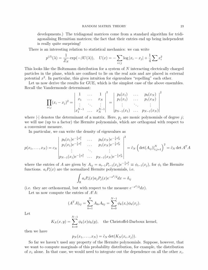
use N1/6 or 2N1/6 instead, depending on how the matrix entries were scaled to begin with).In this case, the asymptotics for the Hermite functions are

φN(x) = π1/42N/2+1/4(N !)1/2N−1/12(Ai(t) +O(N−2/3)

),

where Ai(t) is the Airy function: it satisfies y′′ = ty and y(+∞) = 0 (plus some normalizationconstraint, since this is a second-order ODE). It can also be defined as a contour integral

Ai(t) =1

2πi

∫exp(−tu+ u3/3)du

where the integral is over two rays r(e−π/3) from ∞ to 0, then reπ/3 from 0 to ∞. (Thisintegral naturally arises when the asymptotics of Hermite polynomials are derived through


the steepest descent formula. The Airy function can be also defined as a particular case ofBessel functions, or as a real integral of cos(tu + u3/3). Note, however, that this integral isdifficult to compute since it has a singularity as u→∞.)

Figure 6. The scaled Hermite function (solid line, N=100) and the Airyfunction (dashed line)

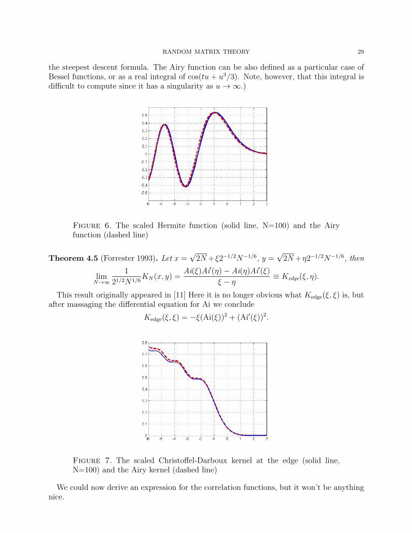
Theorem 4.5 (Forrester 1993). Let x =√

2N+ξ2−1/2N−1/6, y =√

2N+η2−1/2N−1/6, then

limN→∞

1

21/2N1/6KN(x, y) =

Ai(ξ)Ai′(η)− Ai(η)Ai′(ξ)

ξ − η≡ Kedge(ξ, η).

This result originally appeared in [11] Here it is no longer obvious what Kedge(ξ, ξ) is, butafter massaging the differential equation for Ai we conclude

Kedge(ξ, ξ) = −ξ(Ai(ξ))2 + (Ai′(ξ))2.

Figure 7. The scaled Christoffel-Darboux kernel at the edge (solid line,N=100) and the Airy kernel (dashed line)

We could now derive an expression for the correlation functions, but it won’t be anythingnice.


People often care more about the Wishart ensemble, i.e., the matrices of the form X tXwhere X are complex or real Gaussian matrices. In that case, the story is similar but weuse Laguerre polynomials instead of Hermite ones.

Suppose that we want to know the distribution of the largest eigenvalue λmax. Then

P(λmax < 2√N + ξN−1/6) = P(no eigenvalues in [2

√N + ξN−1/6,∞))

= A0[2√N + ξN−1/6,∞) = det(I −KN)

(the Fredholm determinant), where KN is a kernel operator on L2[2√N + ξN−1/6,∞). It is

plausible (although we won’t go into the technical details) that this should converge, afterthe appropriate change of variables, to

det(I −Kedge)

where Kedge is the operator with kernel Kedge(x, y) acting on L2[ξ,∞). This sort of thingcan be tabulated, and is called the Tracy-Widom distribution for β = 2. It turns out(Bornemann, arxiv:0904.1581) that for numerical computations the integral operator can beapproximated by a sum, which makes the computation manageable. An alternative methoduses differential equations developed by Tracy and Widom (arxiv:hep-th/9211141), whichare related to Painleve differential equations.

4.4. Steepest descent method for asymptotics of Hermite polynomials. The asymp-totics for Hermite, Laguerre and other classical orthogonal polynomials are derived using thesteepest descent method. Morally, steepest descent is a way to compute the asymptotics forcontour integrals of the form ∫

C

etf(z)dz

as t → ∞. The idea is to change the contour so that it passes through the critical pointswhere f ′(z) = 0; with luck, the portions of the contour near these points give the largestcontribution to the integral.

More precisely: Let z0 be s.t. f ′(z0) = 0, and write

f(z) = f(z0)−1

2A(eiθ/2(z − z0))2 + . . .

Then necessarily z0 is a saddle point for |f(z)|. Change the contour to go along the line ofsteepest descent through z0. It is then plausible that the contour integral away from z0 isnegligibly small.

Formally, we parametrize u = eiθ/2(z − z0), then∫C

etf(z)dz ≈ etf(z0)e−iθ/2∫C

e−tA/2u2

du ≈ etf(z0)e−iθ/2√

2π

tA

for large t, because this is essentially the Gaussian integral. Recalling that −Aeiθ is thesecond derivative, we have ∫

C

etf(z)dz ≈ etf(z0)

√2π

−tf ′′(z0).

This approximation will hold if the original contour integral can be approximated by integralsin the neighborhood of critical points.

http://arxiv.org/pdf/0904.1581v5.pdf

http://arxiv.org/pdf/hep-th/9211141.pdf


The steepest descent calculations can be carried through identically for asymptotics of∫etf(z)h(z)dz, where h is sufficiently smooth near the critical points; we will simply pick up

an extra factor: ∫C

h(z)etf(z)dz ≈ h(z0)etf(z0)

√2π

−tf ′′(z0).

For a more detailed and rigorous discussion see Chapter 5 in de Bruijn’s book [6], or Copson[5], or any other text on asymptotic methods.

For Hermite polynomials, we have the recurrence relation

xHn(x) =1

2Hn+1(x) + nHn−1(x)

Remark. All families of orthogonal polynomials have some three-term recurrence of thisform (with some function C(n) instead of n above); however, usually it is hard to computeexplicitly. It is the fact that we can do it for the classical polynomials (like Hermite, Laguerre,Jacobi) that makes the steepest descent method possible.

Let

g(t) =∞∑k=0

Hk(x)

k!tk

be the generating function of the Hermite polynomials, then the above recurrence gives

g′(t) = (2x− 2t)g(t) =⇒ g(t) = e2xt−t2

.

Since the Hermite polynomials are coefficients of the Taylor expansion of this, we have (bythe residue formula)

Hn(x) =n!

2πi

∫|z|=1

e2xz−z2

zn+1dz =

n!

2πi

∫|z|=1

exp(2xz − z2 − (n+ 1) log z)dz

Let z = z/√

2n, y = x/√

2n, then the above integral becomes

cn

∫|z|=1

enf(z)dz

z, f(z) = 4yz − 2z2 − log z

We can change the contour to be |z| = 1, because the only singularity is at the origin. Wehave

f ′(z) = 4y − 4z − 1

z,

so the critical points satisfy the equation

f ′(z0) = 0, that is, z20 − yz0 +1

4= 0

This gives rise to three different asymptotics: |y| > 1 (the two real roots case), |y| < 1 (thetwo complex roots case), and y = ±1 (the double root case).

The case of two real roots gives something exponentially small, and we are not muchinterested in it here. The case of y = 1 gives f ′′(z) = 0, so steepest descent as we describedit is not applicable. Instead, there is a single cubic singularity, and changing a contourthrough it appropriately will give the Airy function asymptotics.

If |y| < 1 and we have two complex critical points z0 = 12(y ± i

√1− y2) = 1

2e±iθc , we

deform the contour as below:


z+

z−

θc

Figure 8. Deformed contour going through the two critical points

The steepest descent formula will have two terms, one for each critical point. At criticalitywe have

f(z0) = y2 ± iy√

1− y2 +1

2+ log 2∓ iθc

and therefore,

Hn(√

2ny) ≈ cn

(eny

2exp(in(y

√1− y2 − θc))√

−nf ′′(z+)+eny

2exp(−in(y

√1− y2 − θc))√

−nf ′′(z−)

)where θc = cos−1(y); rewriting, we get

Hn(√

2ny) ≈ cneny2 cos

(n(y√

1− y2 − θc) + θ0

)(where the θ0 comes from

√−nf ′′(z±)).

The asymptotic regime we were considering was√

2ny = ξ√2n

. This gives y = ξ/(2n)

very small. In particular, eny2

= eξ2/4n = 1 + ξ2

4n+ O(n−2), y

√1− y2 = ξ

2n+ O(n−2), and

θc = cos−1(y) ≈ π2− xi

2n+O( 1

n2 ). We can also check that θ0 = O(n−1). Consequently,

Hn

(ξ√2n

)= cne

ξ2/4n cos(ξ − nπ/2 +O(n−1))

which is the asymptotic we had before. (The exponential factor upfront is due to the factthat here we were approximating Hermite polynomials rather than Hermite functions.)


5. Further developments and connections

5.1. Asymptotics of invariant ensembles (Deift et al.) Suppose the eigenvalue dis-

tribution satisfies p(λ1, . . . , λN) = ∆(λ)2 exp(−∑N

i=1 V (λi)) for some potential function V .Here, ∆ is the Vandermonde determinant we had before. The asymptotics for this distri-bution would follow from asymptotics for a family of orthogonal polynomials with weightexp(−V (x))dx.

The difficulty is that there is no explicit formula for the coefficients in the three-termrecurrence relation for these polynomials.

Deift et al. found a way to find these asymptotics (see Chapter 7 in [7] or Section 6.4in Kuijlaars’ review arxiv:1103.5922); the solution method is related to a multidimensionalversion of the Riemann-Hilbert problem.

The Riemann-Hilbert problem is as follows. Consider a contour Σ on C. We would liketo find two functions Y±(z) : C → Cn (for the classical Riemann-Hilbert problem, n = 1),which are analytic on the two regions into which Σ partitions C, and with the property thatY+(z) = V (z)Y−(z) on Σ, for some matrix V . (There will also be some conditions on thebehaviour of Y at infinity.) It turns out that for n > 1 this can be constructed so that oneof the components of Y gives the orthogonal polynomials we want. Deift et al. found a wayto analyze the asymptotics of these solutions.

5.2. Dyson Brownian motion. Suppose that the matrix entries Xij follow independentOrnstein-Uhlenbeck processes.

Remark. An Ornstein-Uhlenbeck process satisfies the stochastic differential equation (SDE)

dxt = −θ(xt − µ)dt+ σdWt,

where W is a Brownian motion. It has a stationary distribution, which is Gaussian centeredon µ with variance σ2

2θ. Such a process can be used to model, e.g., the relaxation of a spring

in physics (normally exponential) in the presence of thermal noise. We will undoubtedlyassume µ = 0 (i.e., Xij centered on 0), and possibly σ = 1.

The eigenvalues, being differentiable functions of the matrix entries Xij, will then alsofollow a diffusion process. Applying Ito’s formula (nontrivially), this can be found to be

dλi =1√NdBi +

(−β

4λi +

β

2N

∑i 6=j

1

λi − λj

), i = 1, . . . , N

Here, Bi are Brownian motions, and β = 1, 2, 4 according to whether the ensemble isorthogonal, unitary, or symplectic. The best introduction is Dyson’s original paper [9].A system of coupled SDE’s is not trivial to solve, but it turns out that the distribu-tion of the solution converges to an equilibrium distribution. One could ask, e.g., aboutthe speed of convergence. This material is covered in Laszlo Erdos’s lecture notes, http://www.mathematik.uni-muenchen.de/~lerdos/Notes/tucson0901.pdf.

5.3. Connections to other disciplines. The methods that were initially developed forrandom matrices have since been used in various other places.

http://arxiv.org/abs/1103.5922

http://www.mathematik.uni-muenchen.de/~lerdos/Notes/tucson0901.pdf

http://www.mathematik.uni-muenchen.de/~lerdos/Notes/tucson0901.pdf


5.3.1. Longest increasing sequence in a permutation (Baik-Deift-Johansson). Consider a per-mutation in Sn, e.g. π ∈ S4 which maps 1234 to 1324. We define l(π) to be the length ofthe longest increasing subsequence in π; here, l(π) = 3 (corresponding to subsequences 134or 124). We would like asymptotics for l(π), and particularly for its distribution, as n→∞.

We will use the RSK (Robinson-Schensted-Knuth) correspondence between permutationsand pairs of standard Young tableaux. A standard Young tableau is the following object.First, partition n, i.e. write it as n = λ1 + λ2 + . . . + λr, where λi are integers, andλ1 ≥ λ2 ≥ . . . ≥ λr > 0. E.g., for n = 10 we might write 10 = 5 + 3 + 2. We then draw thecorresponding shape, where the λi are row lengths:

To turn this into a standard Young tableau, we will fill it with numbers 1, . . . , n whichincrease along rows and along columns. The RSK correspondence asserts that there is abijection between permutations π and pairs of standard Young tableaux of the same shape.For example, there is a permutation π ∈ S10 corresponding to the pair

P =1 2 5 6 83 4 79 10

Q =1 3 5 7 92 4 68 10

The length l(π) is the length of the top row of the standard Young tableau. We define alsor(π) the number of columns in the standard Young tableau; this is the length of the longestdecreasing subsequence in π.

Standard Young tableaux have been well-studied because of their relationship to repre-sentations of Sn. See for example W. Fulton. Young Tableaux. Cambridge University Press1997.

To get the distribution of l(π), we need to count the number of standard Young tableauxwith a given length of the top row. Now, there is a formula, due to Frobenius and Young,for the number f(λ) of standard Young tableaux of a given shape λ (this is, by the way, thedimension of the corresponding irreducible representation of Sn). (Here, λ is a partition ofn, that is, n = λ1 + . . .+ λr with λ1 ≥ λ2 ≥ . . . ≥ λr > 0.)

Let hi = λi + (r − i), then the Frobenius-Young formula asserts

f(λ) = n!∏i>j

(hi − hj)r∏i=1

1

hi!

Remark. The formula which tends to get taught in combinatorics classes is the hook lengthformula: for each position x in the standard Young tableau, let hook(x) count the numberof cells to the right of it, plus the number of cells below it, plus 1 for x itself. Thenf(λ) = n!/

∏x hook(x), but this isn’t very useful for us. (It is useful in other contexts. For

example, Vershik and Kerov used this formula to obtain the asymptotic shape of a typicalstandard tableau.)


In particular, by the RSK correspondence the number of permutations π with r(π) = rwill be

(n!)2∑

h1,...,hr:∑hi=n+

r(r−1)2

∏i<j

(hi − hj)2r∏i=1

1

(hi!)2

Since the product∏

(hi − hj)2 is related to the Vandermonde determinant, we get the con-nection to orthogonal polynomials and then to random matrices.

5.3.2. Last passage percolation. Consider a square M ×N lattice (with (M + 1)× (N + 1)points), with weights wij in vertices. We will take wij to be iid geometric, i.e.

P(wij = k) = (1− q)qk.We would like to find a path from (0, 0) to (M,N) which moves only up and to the right,and which maximizes the sum

∑wij of the weights it passes through. Let

G(N,M) = maxp:path up and right

∑wij

be this maximum.Note that W is a matrix of nonnegative integers. We can write a generalised permutation

corresponding to it: the permutation π will contain the pair(ij

)wij times. For example,

W =

1 2 00 3 01 1 01 0 1

, π =

(1 1 1 2 2 2 3 3 4 41 2 2 2 2 2 1 2 1 3

)

Then the optimal path corresponds to the longest nondecreasing subsequence in π, and π (viathe RSK correspondence – in fact, this was Knuth’s contribution) corresponds to a pair ofsemistandard Young tableaux: the semistandard Young tableaux are filled by the top, resp.the bottom, row of π, and the numbers must be increasing along rows and nondecreasingalong columns. Semistandart Young tableaus can be counted similarly to standard ones; thepolynomials that arise are called the Meixner orthogonal polynomials.

5.3.3. Other problems. We don’t have time to mention these in any detail, but there aretotally asymmetric exclusion processes, Aztec diamond domino tilings, and viscious walkers.Most of the work on the topics in this section has been done by Johansson and his co-authors,and the best place to find out more is to read his papers, for example, [2], [14], [15], [16].

References

[1] Greg W. Anderson, Alice Guionnet, and Ofer Zeitouni. An Introduction to Random Matrices, volume118 of Cambridge studies in advanced mathematics. Cambridge University Press, 2009.

[2] Jinho Baik, Percy Deift, and Kurt Johansson. On the distribution of the length of the longest increasingsubsequence of random permutations. Journal of the American Mathematical Society, 12:1119–1178,1999.

[3] S. G. Bobkov and F. Gotze. Exponential integrability and transportation cost related to logarithmicSobolev inequalities. Journal of Functional Analysis, 163:1–28, 1999.

[4] Kai Lai Chung. A Course in Probability Theory. Academic Press, third edition, 2001.[5] E. T. Copson. Asymptotic expansions. Cambridge Tracts in Mathematics and Mathematical Physics.

Cambridge University Press, 1967.


[6] N. G. de Bruijn. Asymptotic methods in analysis. A Series of Monographs on Pure and Applied Math-ematics. North Holland Publishing Co., 1958.

[7] Percy Deift. Orthogonal Polynomials and Random Matrices: A Riemann-Hilbert Approach, volume 3 ofCourant Lecture Notes in Mathematics. Courant Institute of Mathematical Sciences, 1999.

[8] Ioana Dumitriu and Alan Edelman. Matrix models for beta ensembles. Journal of Mathematical Physics,43:5830–5847, 2008.

[9] Freeman J. Dyson. A Brownian-motion model for eigenvalues of a random matrix. Journal of Mathe-matical Physics, 3:1191–1198, 1962.

[10] Z. Furedi and J. Komlos. The eigenvalues of random symmetric matrices. Combinatorica, 1:233–241,1981.

[11] P. J. Forrester. The spectrum edge of random matrix ensembles. Nuclear Physics B, 402:709–728, 1993.[12] Leonard Gross. Logarithmic sobolev inequalities and contractivity properties of semigroups. volume

1563 of Lecture Notes in Mathematics, pages 54–88. Springer, 1993.[13] J. Ben Hough, Manjunath Krishnapur, Yuval Peres, and Balint Virag. Determinantal processes and

independence. Probability Surveys, 3:206–229, 2006.[14] Kurt Johansson. Shape fluctuations and random matrices. Communications in Mathematical Physics,

209:437–476, 2000.[15] Kurt Johansson. Discrete orthogonal polynomial ensembles and the Plancherel measure. Annals of

Mathematics, 153:259–296, 2001.[16] Kurt Johansson. Non-intersecting paths, random tilings and random matrices. Probability Theory and

Related Fields, 123:225–280, 2002.[17] N. El Karoui. Spectrum estimation for large dimensional covariance matrices using random matrix

theory. Annals of Statistics, 36:2757–2790, 2008.[18] Michael Reed and Barry Simon. Methods of Mathematical Physics IV: Analysis of Operators. Academic

Press, 1978.[19] Ya. Sinai and A. Soshnikov. Central limit theorem for traces of large random matrices with independent

matrix elements. Boletim de Sociedade Brasiliera de Matematica, 29:1–24, 1998.[20] Alexander Soshnikov. Universality at the edge of the spectrum in Wigner random matrices. Communi-

cations in Mathematical Physics, 207:697–733, 1999.[21] Alexander Soshnikov. Determinantal random point fields. Russian Mathematical Surveys, 55:923–975,

2000.[22] Gabor Szego. Orthogonal Polynomials. American Mathematical Society, third edition, 1967.[23] A. W. van der Vaart. Asymptotic Statistics. Cambridge University Press, 1998.

Documents

RANDOM MATRIX THEORY - staff.math.su.sestaff.math.su.se/shapiro/UIUC/random_matrices.pdfRANDOM MATRIX THEORY SLAVA KARGIN STATISTICAL LABORATORY, UNIVERSITY OF CAMBRIDGE [email protected]