Embed Size (px)
Citation preview
Random Matrix Theory
What is a Random Matrix? A matrix whose elements xi j are random
variables
x11 x12 · · · x1p
x21 x22 · · · x2p...
.... . .
...
xp1 xp1 · · · xpp
What is a random variable? A quantity whose value is random and to
which a probability distribution is assigned
RV Example (discrete): Number of siblings
x 0 1 2 3 . . .
P r 0.28 0.3 0.24 0.08 . . .
1
Random Matrix Theory
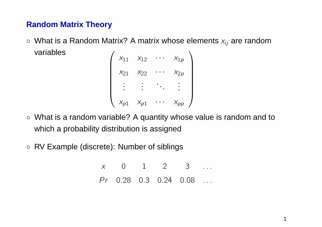
RV Example (continuous): Annual teaching income across US
Probability distribution function (pdf)of teachers’ salaries across US
40,000 100,000
x~
2
Random Matrix Theory
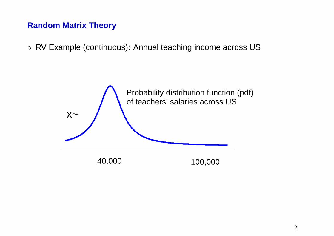
Natural tools which helps us explore relationships between RVs
RM Example: education (x1) and income (x2)
Inco
me
years education
This relationship can be express as a random matrix
var [x1] cov [x1, x2]
cov [x2, x1] var [x2]
3

Random Matrix Theory
Other applications:
Wireless communications
Nuclear physics
Finance
Genetics
. . .
4
Rare events in nonlinear lightwave systems
Elaine T. Spiller
SAMSI and Duke University
SAMSI/CRSC undergraduate workshop - May 21, 2007
5
Communications
Goal
send lots of information very quickly over very long distances
make almost no mistakes
Optical Communications
use light to represent information
transmit light (information) through fiber
Our goal
model this system mathematically
calculate the probability errors
6
Very brief history of optical fiber communications
Fiber Optic Communication: The transmission of information via a
signal comprised of light that travels through glass fiber which acts as a
wave guide.
made possible by laser (1960) and
low-loss, single-mode fiber (1970)
nonlinear Schrodinger equation exactly solvable by the inverse
scattering transform: Zakharov and Shabat, (1971)
NLS proposed for fibers by Hasegawa and Tappert, (1973)
experimental verification by Mollenauer, (1983)
made practical by advent of in-line fiber amplifiers (1988)
7
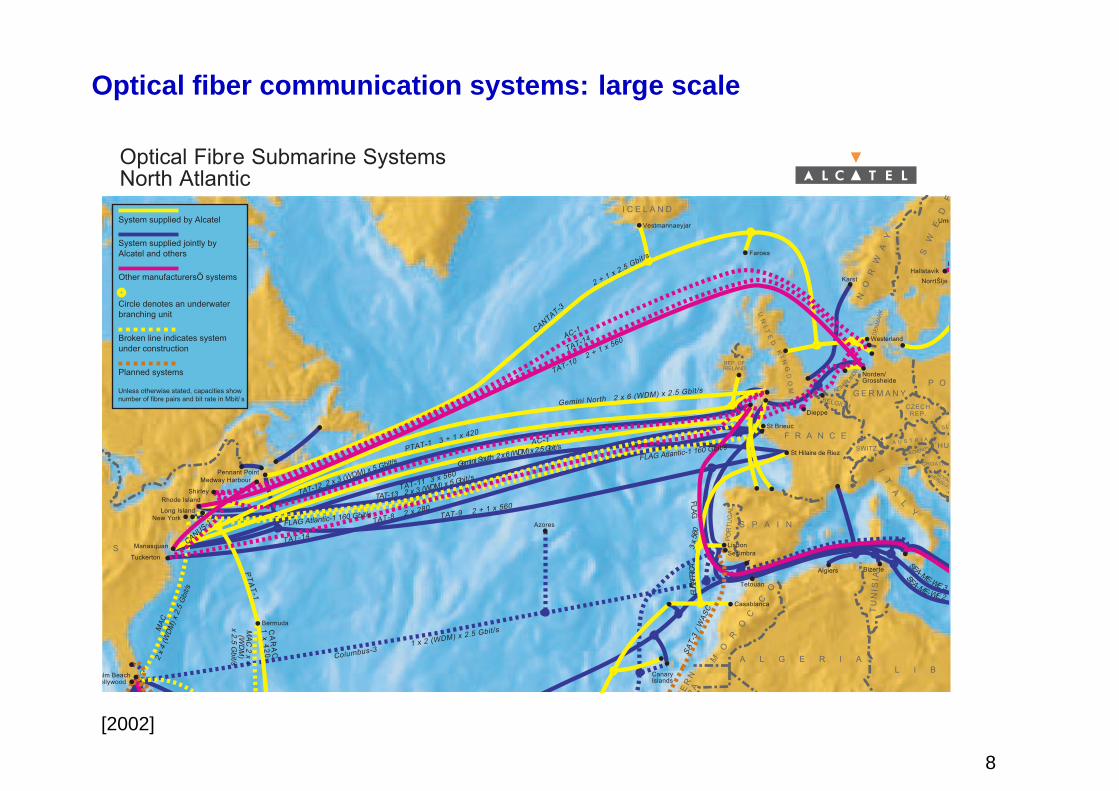
Optical fiber communication systems: large scale
BELGIUM
P OG E R M A N YNETHE
RL
ANDS
A U S T R I A
CZECHREP.
DE
NM
AR
K
IT
AL
Y
SWITZ.
BOSNIA-
HERZEGOVINA
SLOVENI A HU
SLO
F R A N C E
S P A I N
PO
RT
UG
AL
I C E L A N D
NO
RW
AY
SW
ED
E
E S
C A N A D A
A L G E R I AMO
RO
C
CO
TE
RN
RA
L I B
TU
NIS
IA
REP. OFIRELAND
UN
IT
ED
KI
NG
DO
M
CROATIAGemini South 2x6 (WDM) x 2.5Gbit/s
FLAG
EURA
FRIC
A3
x56
0
CANUS-1
TAT-11 3 x 560
TAT-12 2 x 3 (WDM) x 5 Gbit/s
PTAT-1 3 + 1 x 420
Gemini North 2 x 6 (WDM) x 2.5 Gbit/s
AC-1
FLAG Atlantic-1 160 Gbit/s
TAT-9 2 + 1 x 560
Columbus-3 1 x 2 (WDM) x 2.5 Gbit/s
TAT-8 2 x 280
TAT-13 2 x 3 (WDM) x 5 Gbit/s
TAT-14
MA
C 2 x 4
(WD
M)
x 2.5 Gbit/s
MA
C
2 x
4 (W
DM
) x 2
.5 G
bit/s
CANTAT-3
2 + 1 x 2.5 Gbit/s
TAT-10 2 + 1 x 560
TAT-14AC-1
6
SEA-ME-WE 2
SEA-ME-WE 3
CA
RA
C
1 x
42
0
PT
AT
-1
SA
T-3
/ W
AS
C
FLAG Atlantic-1 160 Gbit/s
Casablanca
Lisbon
St Hilaire de Riez
Sesimbra
Tetouan
Algiers Bizerte
CanaryIslands
Vestmannaeyjar
Faroes
Westerland
Bermuda
Azores
Medway Harbour
Manasquan
Pennant Point
Rhode IslandShirley
Long IslandNew York
Tuckerton
est Palm BeachHollywood
Ume
Dieppe
St Brieuc
HallstavikKarst
Norden/Grossheide
NorrtŠlje
System supplied by Alcatel
Circle denotes an underwater branching unit
Broken line indicates system under construction
Planned systems
Other manufacturersÕ systems
System supplied jointly byAlcatel and others
Unless otherwise stated, capacities show number of fibre pairs and bit rate in Mbit/ s
Optical Fibre Submarine Systems North Atlantic
[2002]
8
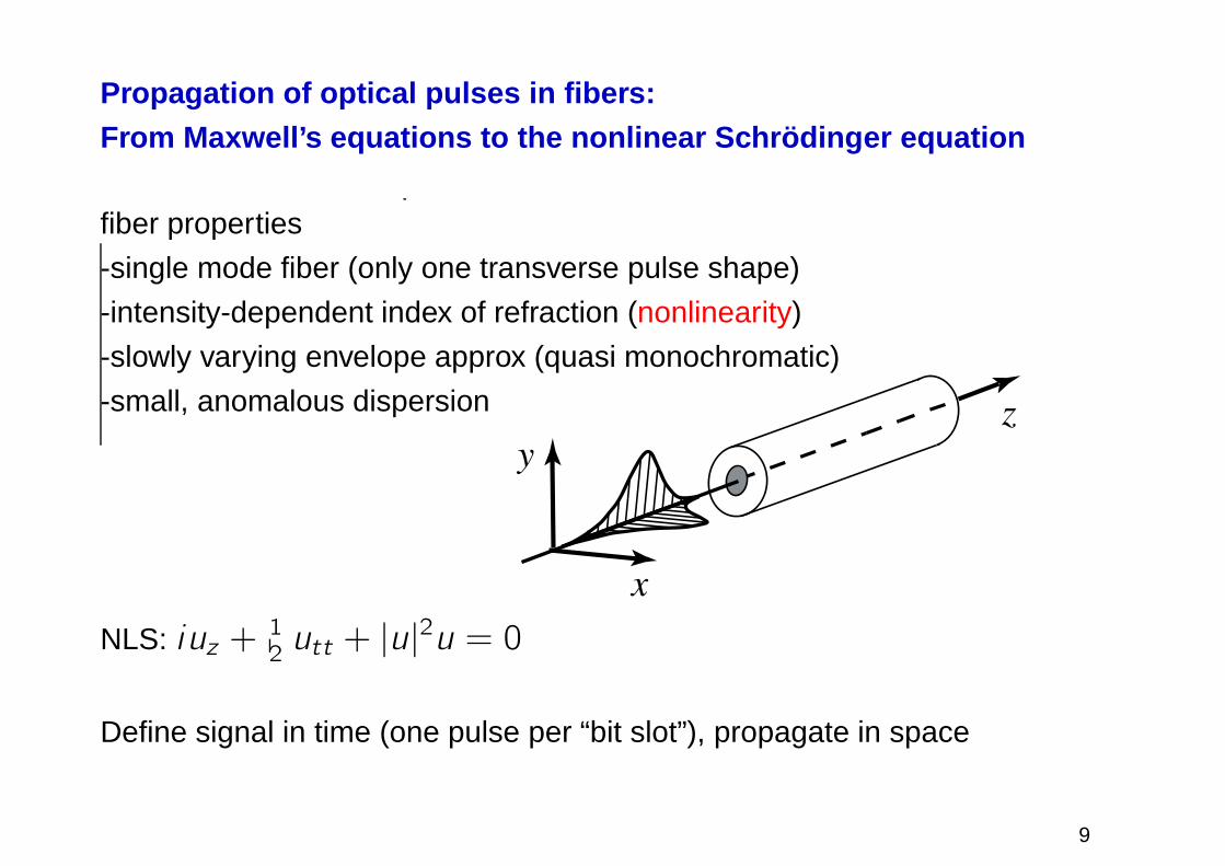
Propagation of optical pulses in fibers:From Maxwell’s equations to the nonlinear Schr odinger equation
fiber properties
-single mode fiber (only one transverse pulse shape)
-intensity-dependent index of refraction (nonlinearity)
-slowly varying envelope approx (quasi monochromatic)
-small, anomalous dispersion
x
y
z
NLS: iuz +1
2utt + |u|
2u = 0
Define signal in time (one pulse per “bit slot”), propagate in space
9
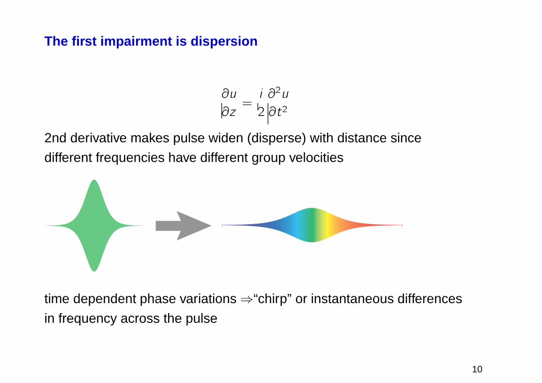
The first impairment is dispersion
∂u
∂z=i
2
∂2u
∂t2
2nd derivative makes pulse widen (disperse) with distance since
different frequencies have different group velocities
time dependent phase variations⇒“chirp” or instantaneous differences
in frequency across the pulse
10
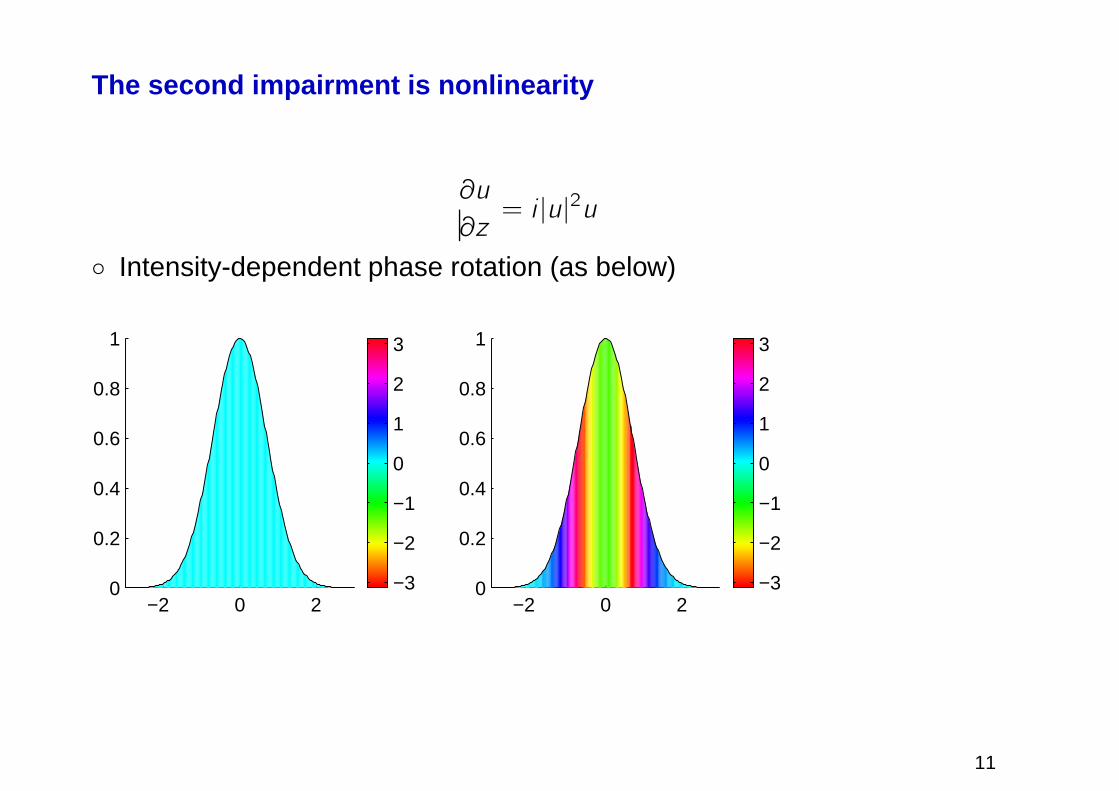
The second impairment is nonlinearity
∂u
∂z= i |u|2u
Intensity-dependent phase rotation (as below)
−3
−2
−1
0
1
2
3
−2 0 20
0.2
0.4
0.6
0.8
1
−3
−2
−1
0
1
2
3
−2 0 20
0.2
0.4
0.6
0.8
1
11
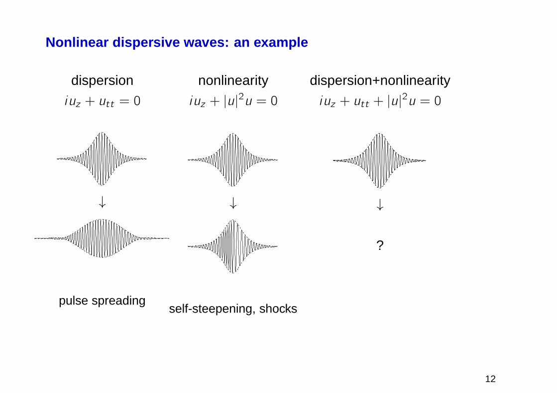
Nonlinear dispersive waves: an example
dispersion
iuz + utt = 0
↓
pulse spreading
nonlinearity
iuz + |u|2u = 0
↓
self-steepening, shocks
dispersion+nonlinearity
iuz + utt + |u|2u = 0
↓
?
12
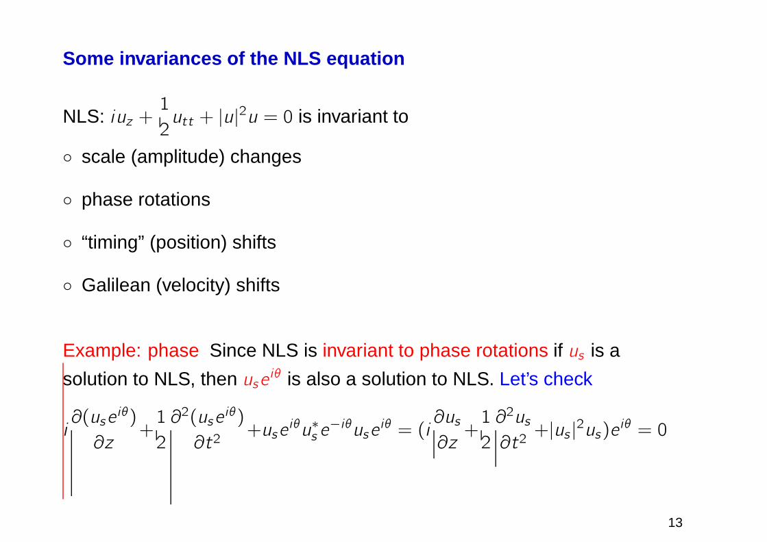
Some invariances of the NLS equation
NLS: iuz +1
2utt + |u|
2u = 0 is invariant to
scale (amplitude) changes
phase rotations
“timing” (position) shifts
Galilean (velocity) shifts
Example: phase Since NLS is invariant to phase rotations if us is a
solution to NLS, then use iθ is also a solution to NLS. Let’s check
i∂(use
iθ)
∂z+1
2
∂2(useiθ)
∂t2+use
iθu∗s e−iθuse
iθ = (i∂us∂z+1
2
∂2us∂t2+|us |
2us)eiθ = 0
13
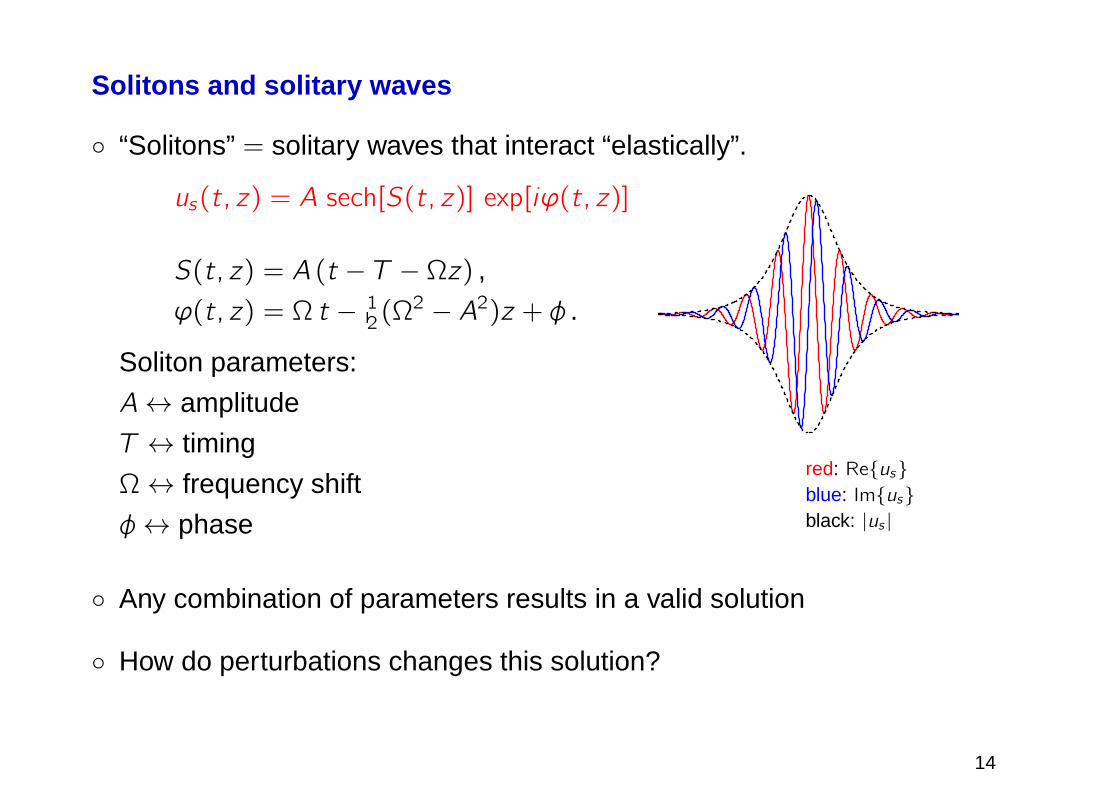
Solitons and solitary waves
“Solitons” = solitary waves that interact “elastically”.
us(t, z) = A sech[S(t, z)] exp[iϕ(t, z)]
S(t, z) = A (t − T −Ωz) ,
ϕ(t, z) = Ω t − 12(Ω2 − A2)z + φ .
Soliton parameters:
A↔ amplitude
T ↔ timing
Ω↔ frequency shift
φ↔ phase
red: Reusblue: Imusblack: |us |
Any combination of parameters results in a valid solution
How do perturbations changes this solution?
14
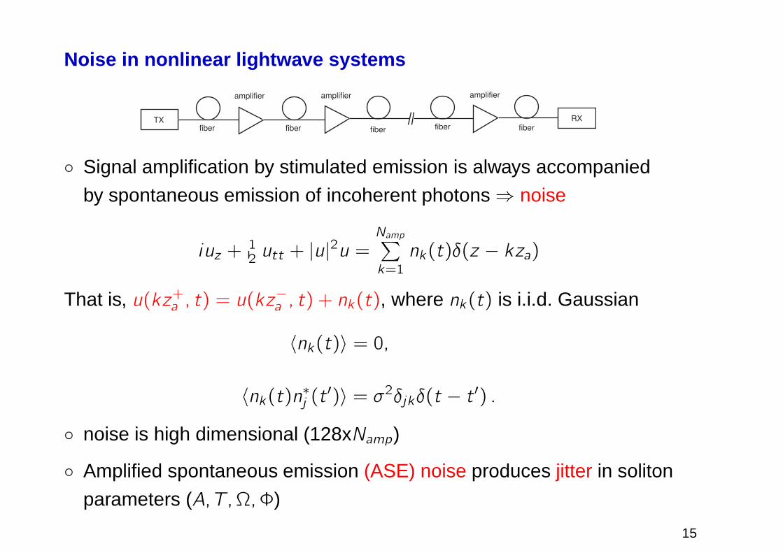
Noise in nonlinear lightwave systems
TX RX
fiber fiber fiber fiber fiber
amplifier amplifier amplifier
Signal amplification by stimulated emission is always accompanied
by spontaneous emission of incoherent photons⇒ noise
iuz +1
2utt + |u|
2u =Namp∑
k=1
nk(t)δ(z − kza)
That is, u(kz+a , t) = u(kz−a , t) + nk(t), where nk(t) is i.i.d. Gaussian
〈nk(t)〉 = 0,
〈nk(t)n∗j (t′)〉 = σ2δjkδ(t − t
′) .
noise is high dimensional (128xNamp)
Amplified spontaneous emission (ASE) noise produces jitter in soliton
parameters (A, T,Ω,Φ)
15
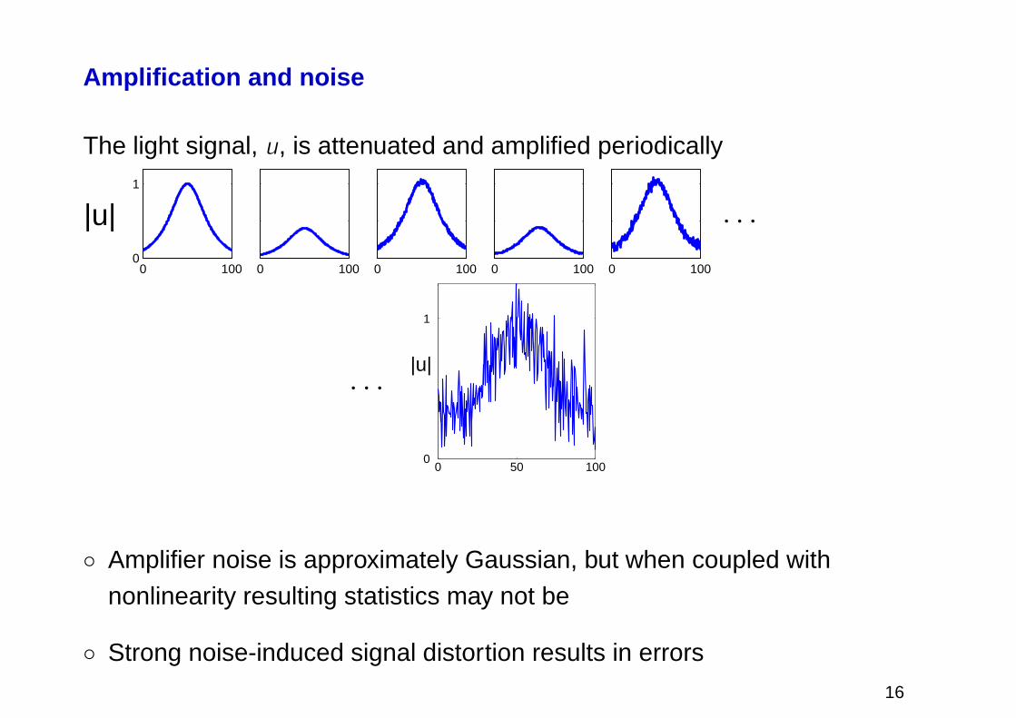
Amplification and noise
The light signal, u, is attenuated and amplified periodically
0 1000
1
|u|
0 100 0 100 0 100 0 100
· · ·
· · ·
0 50 1000
1
|u|
Amplifier noise is approximately Gaussian, but when coupled with
nonlinearity resulting statistics may not be
Strong noise-induced signal distortion results in errors
16
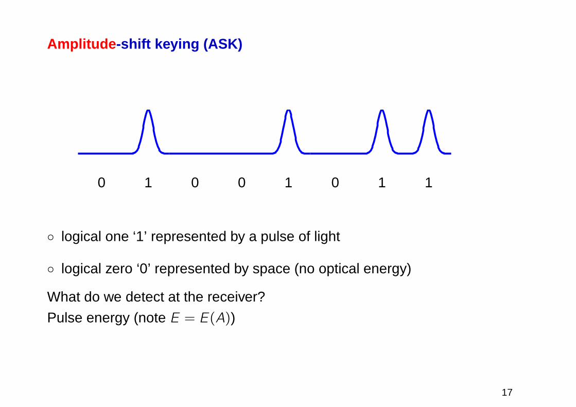
Amplitude -shift keying (ASK)
0 1 0 0 1 0 1 1
logical one ‘1’ represented by a pulse of light
logical zero ‘0’ represented by space (no optical energy)
What do we detect at the receiver?
Pulse energy (note E = E(A))
17
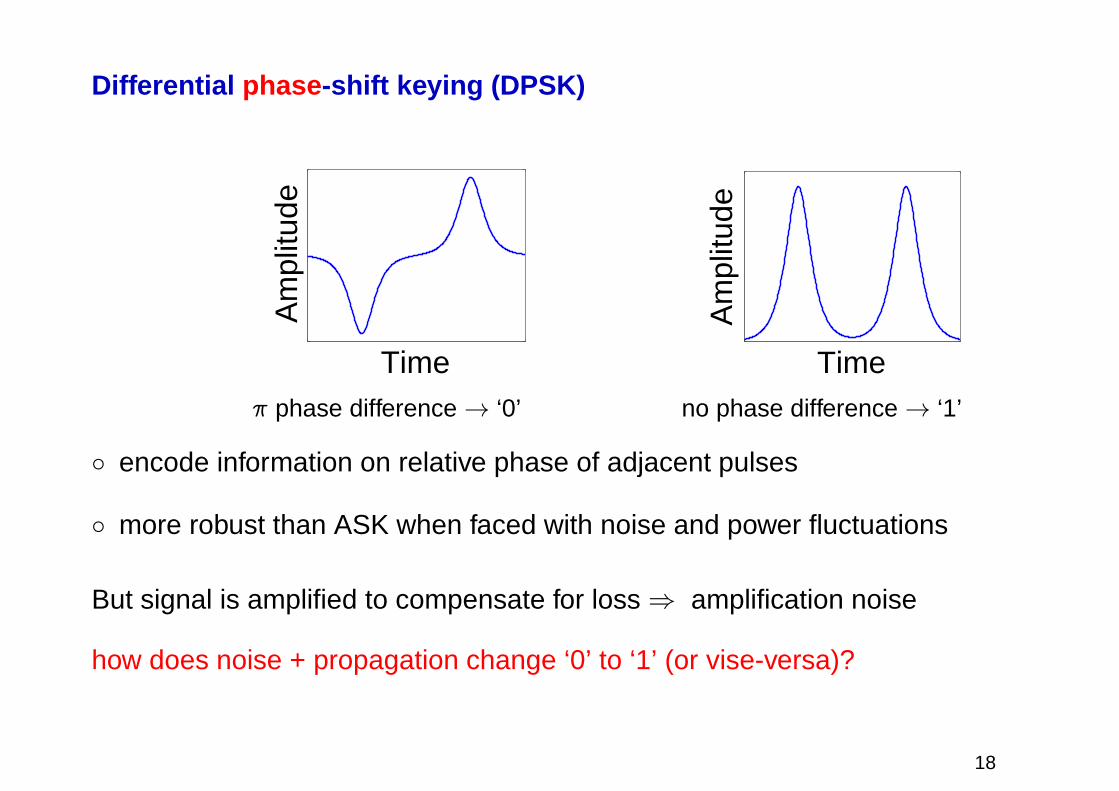
Differential phase -shift keying (DPSK)
Time
Am
plitu
de
Time
Am
plitu
de
π phase difference→ ‘0’ no phase difference→ ‘1’
encode information on relative phase of adjacent pulses
more robust than ASK when faced with noise and power fluctuations
But signal is amplified to compensate for loss⇒ amplification noise
how does noise + propagation change ‘0’ to ‘1’ (or vise-versa)?
18
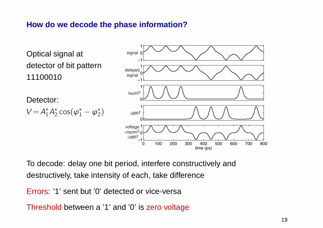
How do we decode the phase information?
Optical signal at
detector of bit pattern
11100010
Detector:
V =A∗1A∗2 cos(ϕ
∗1 − ϕ
∗2)
−1
0
1
−1
0
1
0
1
0
1
0 100 200 300 400 500 600 700 800−1
0
1
time (ps)
signal
delayed
signal
|sum|2
voltage
=|sum|2
-|diff|2
|diff|2
To decode: delay one bit period, interfere constructively and
destructively, take intensity of each, take difference
Errors: ’1’ sent but ’0’ detected or vice-versa
Threshold between a ’1’ and ’0’ is zero voltage
19
Noise-induced errors
Predicting error rates:
Error rates must be small; e.g., 10−9 or 10−12
Simulating rare events with Monte Carlo is prohibitively expensive
Understanding why errors occur:
What combination of impairments produces errors?
If one knows how errors arise, they can potentially be corrected
One way to see errors: use importance sampling to bias simulations
toward these events
Crucial to understand most likely noise realizations that
lead to desired events
Perturbation theory to study noise-induced signal degradation
20
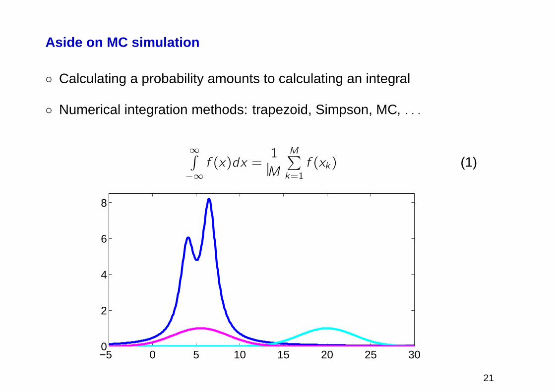
Aside on MC simulation
Calculating a probability amounts to calculating an integral
Numerical integration methods: trapezoid, Simpson, MC, . . .
∞∫
−∞
f (x)dx =1
M
M∑
k=1
f (xk) (1)
−5 0 5 10 15 20 25 300
2
4
6
8
21
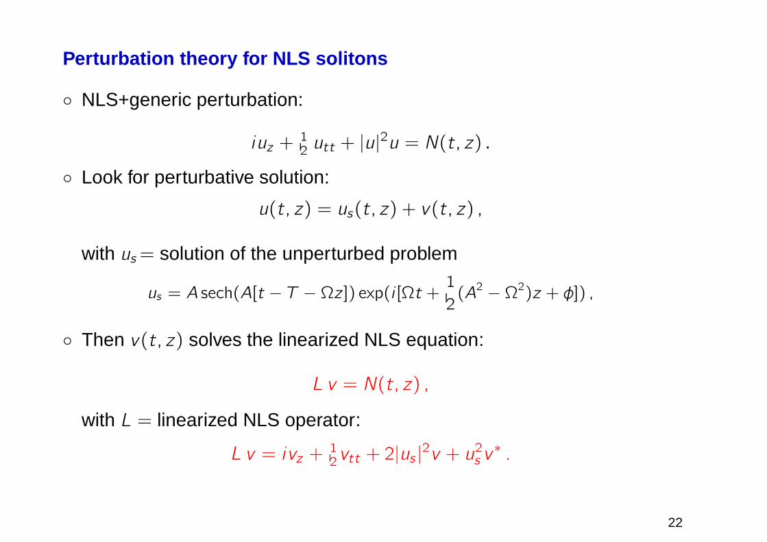
Perturbation theory for NLS solitons
NLS+generic perturbation:
iuz +1
2utt + |u|
2u = N(t, z) .
Look for perturbative solution:
u(t, z) = us(t, z) + v(t, z) ,
with us= solution of the unperturbed problem
us = A sech(A[t − T − Ωz ]) exp(i [Ωt +1
2(A2 −Ω2)z + φ]) ,
Then v(t, z) solves the linearized NLS equation:
L v = N(t, z) ,
with L = linearized NLS operator:
L v = ivz +1
2vtt + 2|us |
2v + u2s v∗ .
22
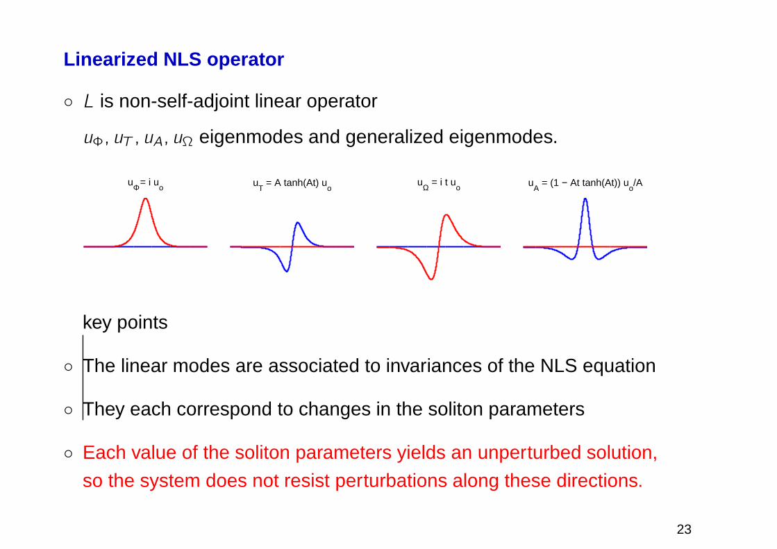
Linearized NLS operator
L is non-self-adjoint linear operator
uΦ, uT , uA, uΩ eigenmodes and generalized eigenmodes.
uΦ = i uo u
T = A tanh(At) u
ouΩ = i t u
o uA = (1 − At tanh(At)) u
o/A
key points
The linear modes are associated to invariances of the NLS equation
They each correspond to changes in the soliton parameters
Each value of the soliton parameters yields an unperturbed solution,
so the system does not resist perturbations along these directions.
23
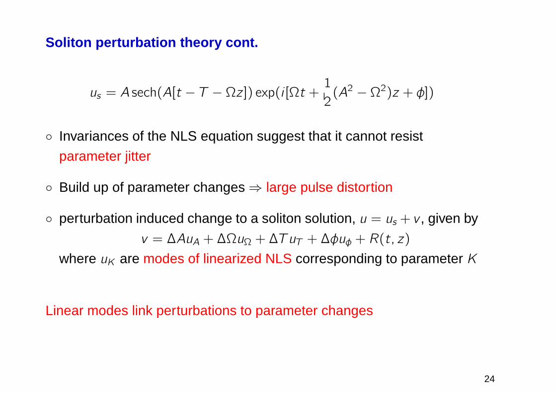
Soliton perturbation theory cont.
us = A sech(A[t − T −Ωz ]) exp(i [Ωt +1
2(A2 −Ω2)z + φ])
Invariances of the NLS equation suggest that it cannot resist
parameter jitter
Build up of parameter changes⇒ large pulse distortion
perturbation induced change to a soliton solution, u = us + v , given by
v = ∆AuA +∆ΩuΩ +∆TuT +∆φuφ + R(t, z)
where uK are modes of linearized NLS corresponding to parameter K
Linear modes link perturbations to parameter changes
24
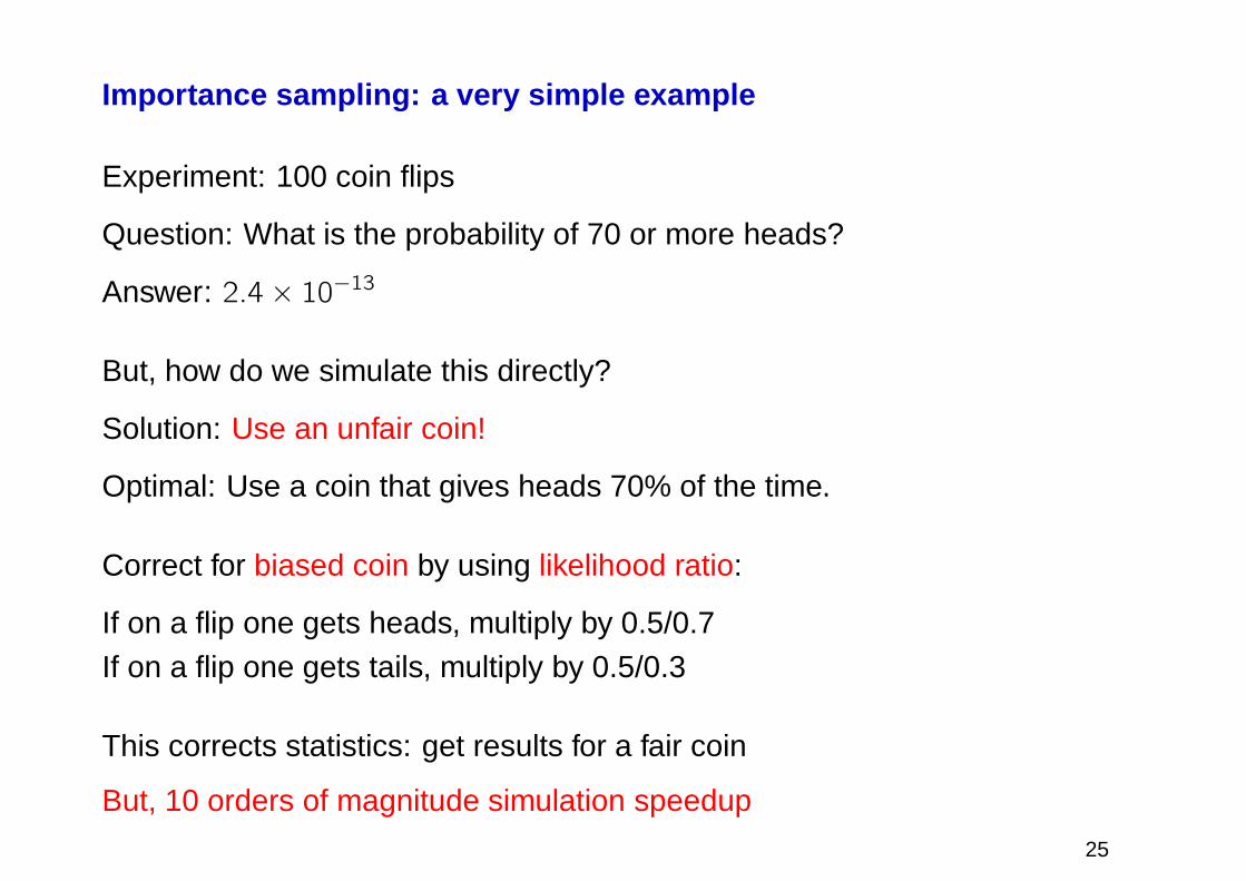
Importance sampling: a very simple example
Experiment: 100 coin flips
Question: What is the probability of 70 or more heads?
Answer: 2.4× 10⁻¹³
But, how do we simulate this directly?
Solution: Use an unfair coin!
Optimal: Use a coin that gives heads 70% of the time.
Correct for biased coin by using likelihood ratio:
If on a flip one gets heads, multiply by 0.5/0.7If on a flip one gets tails, multiply by 0.5/0.3
This corrects statistics: get results for a fair coin
But, 10 orders of magnitude simulation speedup
25
IS application: calculating rare events in nonlinear commu nicationsystems
goals: predict error rates and understand why errors occur
recall: error rates must be small < 10−10
know: how noise changes soliton parameters⇒ linear modes
idea: use linear modes to bias simulations toward rare events of interest
but:Crucial to understand most likely noise realizations that lead to desiredevents, need to be careful
26
Optimal biasing for DMNLS
Consider a noise-induced perturbation, v , to the solution us
v = ∆TuT +∆ΩuΩ +∆φuφ +∆λuλ + R
Bias noise with function of time b(t)
n(t) white, Gaussian i.i.d., v(t) = n(t) + b(t)
Maximize probability of hitting, on average, a desired parameter
change, ∆K, (K ∈ T,Ω, φ, λ)
Solution: b(t) ∝ ∆K uK(t)
27
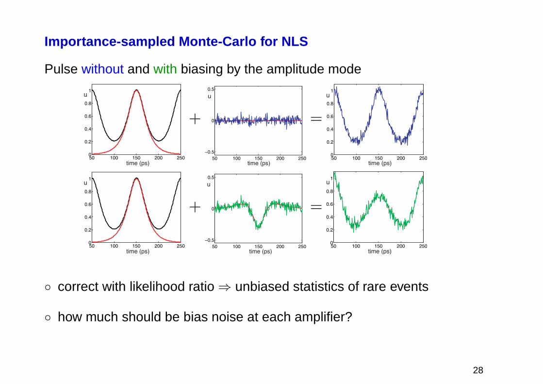
Importance-sampled Monte-Carlo for NLS
Pulse without and with biasing by the amplitude mode
50 100 150 200 2500
0.2
0.4
0.6
0.8
1u
time (ps)
+
50 100 150 200 250
−0.5
0
0.5
u
time (ps)
=
50 100 150 200 2500
0.2
0.4
0.6
0.8
1u
time (ps)
50 100 150 200 2500
0.2
0.4
0.6
0.8
1u
time (ps)
+
50 100 150 200 250
−0.5
0
0.5
u
time (ps)
=
50 100 150 200 2500
0.2
0.4
0.6
0.8
1u
time (ps)
correct with likelihood ratio⇒ unbiased statistics of rare events
how much should be bias noise at each amplifier?
28
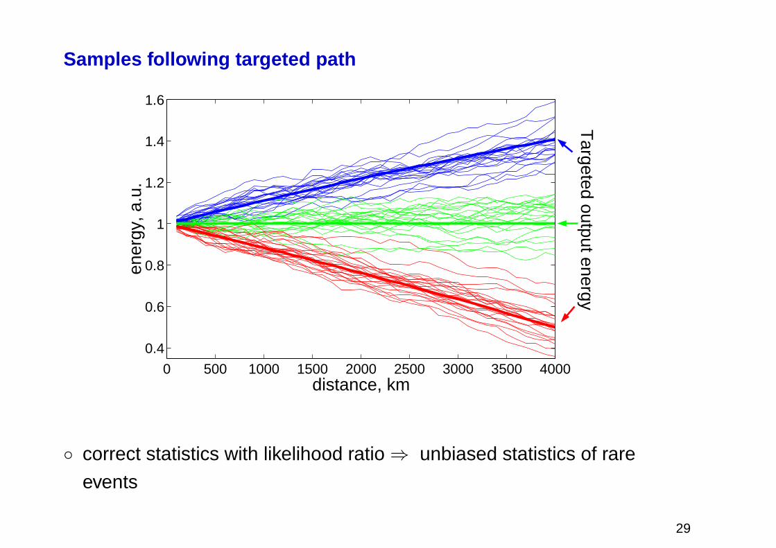
Samples following targeted path
0 500 1000 1500 2000 2500 3000 3500 4000
0.4
0.6
0.8
1
1.2
1.4
1.6
distance, km
ener
gy, a
.u.
Targeted output energy
correct statistics with likelihood ratio⇒ unbiased statistics of rare
events
29
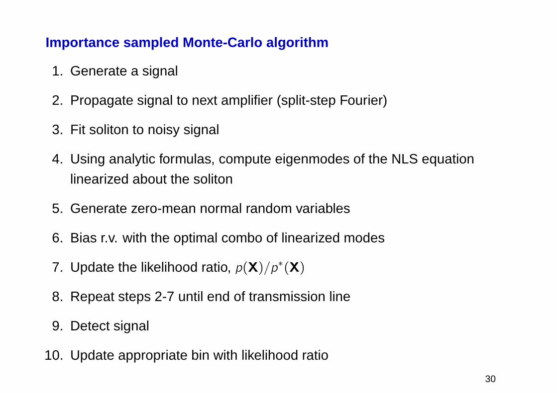
Importance sampled Monte-Carlo algorithm
1. Generate a signal
2. Propagate signal to next amplifier (split-step Fourier)
3. Fit soliton to noisy signal
4. Using analytic formulas, compute eigenmodes of the NLS equation
linearized about the soliton
5. Generate zero-mean normal random variables
6. Bias r.v. with the optimal combo of linearized modes
7. Update the likelihood ratio, p(X)/p∗(X)
8. Repeat steps 2-7 until end of transmission line
9. Detect signal
10. Update appropriate bin with likelihood ratio
30
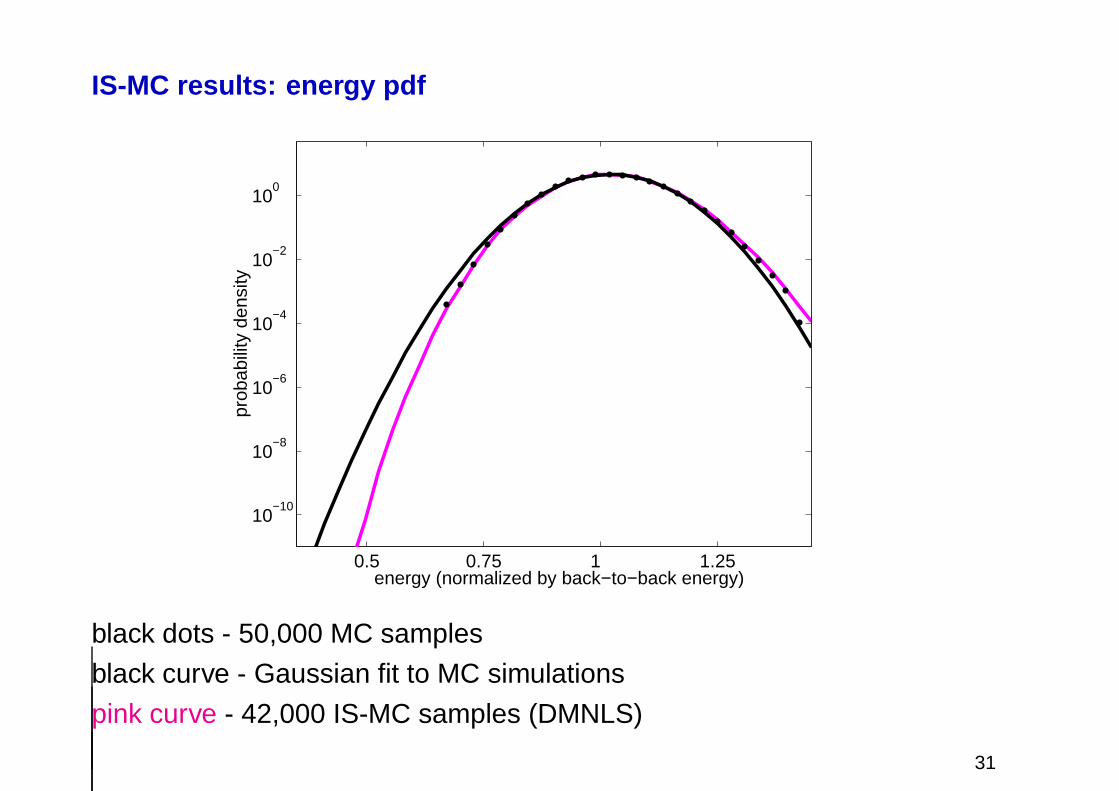
IS-MC results: energy pdf
0.5 0.75 1 1.25
10−10
10−8
10−6
10−4
10−2
100
energy (normalized by back−to−back energy)
prob
abili
ty d
ensi
ty
black dots - 50,000 MC samples
black curve - Gaussian fit to MC simulations
pink curve - 42,000 IS-MC samples (DMNLS)
31
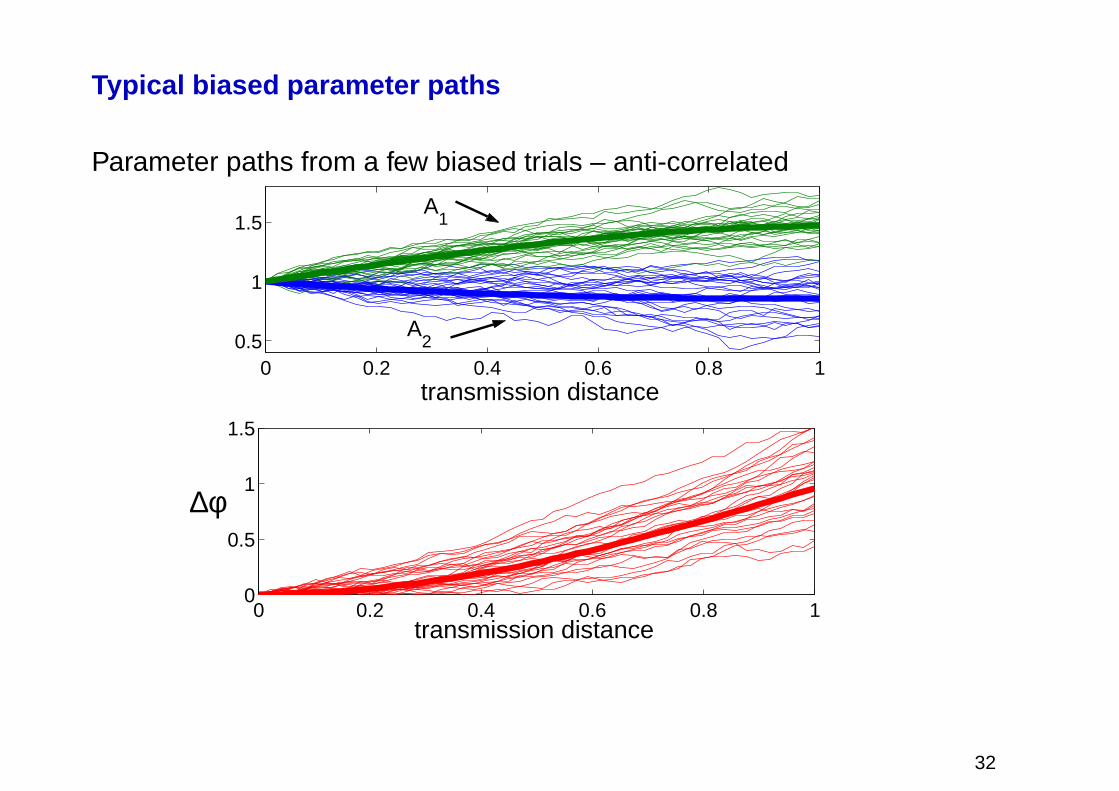
Typical biased parameter paths
Parameter paths from a few biased trials – anti-correlated
0 0.2 0.4 0.6 0.8 10.5
1
1.5
transmission distance
A1
A2
0 0.2 0.4 0.6 0.8 10
0.5
1
1.5
transmission distance
∆φ
32
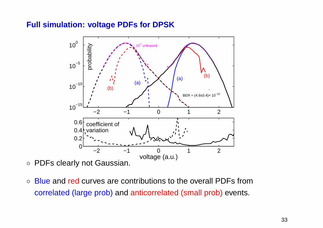
Full simulation: voltage PDFs for DPSK
−2 −1 0 1 210
−15
10−10
10−5
100
prob
abili
ty(b)
(a)(a)
(b)
107 unbiased
BER = (4.9±0.4)× 10−10
−2 −1 0 1 20
0.20.40.6
voltage (a.u.)
coefficient ofvariation
PDFs clearly not Gaussian.
Blue and red curves are contributions to the overall PDFs from
correlated (large prob) and anticorrelated (small prob) events.
33
Rare events in nonlinear lightwave systems
Conclusions
Demonstration of importance sampled Monte-Carlo simulations of
rare events in soliton-based optical communication systems
PDFs can be sampled way down into the tails
Perturbation theory to guide importance sampling
Examples: pdfs of energy and voltage
This method can be used as a practical tool to analyze the
performance of nonlinear optical systems
34