Random KNN - West Virginia Universityjharner/courses/stat623/ICDM2014.pdf · • New Modeling Methods ... >golub.bel

Introduction Classification Variable Selection Regression Parallelization

Random KNN

E. James Harne1, Shengqiao Li2, and Donald A. Adjeroh1

1. West Virginia University

2. University of Pittsburgh Medical Center

ICDM 2014


Outline

Introduction

Classification

Variable Selection

Regression

Parallelization


Challenges and Possible Solutionsfor High-dimensional Data

• Challenges:• Small n, large p• Irrelevant features• Hard to build predictive models directly

• Solutions:• Variable (Feature) Selection:

•Variable filtering (statistic defined over populations): Easy to

compute and fast, but not necessarily good for the final

predictive model.

•Wrapper methods (model wrapped in a search algorithm):

Slow and not scalable, but the final model might be good,

• New Modeling Methods•

Random Forests


Overview

Random KNN consists of an ensemble of base k-nearest neighbormodels, each constructed from a random subset of the inputvariables.

Random KNN can be used to select important features using theRKNN-FS algorithm. RKNN-FS is an innovative feature selectionprocedure for“small n, large p problems.”

Random KNN (no bootstrapping) is fast and stable compared withRandom Forests.

The rknn R package implements Random KNN classification,regression and variable selection algorithms.


Advantages of Random KNN

• KNN is stable, no hierarchical structure

• Final model can be a single KNN (vs. many trees)

• Local method: robust for complex data structure

• Automatically re-train, incremental learning

• Easy to implement


Random KNN PropertiesSymbol Definition

r number of KNN classifersm number of features used for each KNNM multiplicity of a feature in r KNN’s; M ⇠ B(r , m/p)S number of silent features (features not drawn);

P(S = s) =�ps

�Pp�sj=0

(�1)p�s�j (p�sj )(

jm)

r

(pm)r

R number of KNN’s until S = 0If indicator variable, 1 if feature f is silent;

P(If = 1) = P(M = 0) = (1� mp )

r

rf number of KNN’s until f is drawn⌫ ⌫ = E (M) = rm

p

� � = E (S) = p(1� mp )

r

⌘ coverage probability;

P(S = 0) =Pp

j=0

(�1)p�j�pj

� � jm

��pm

��r


Coverage ProbabilityIf we ignore the dependency among If ’s, and approximate S by abinomial random variable B(p, (1�m/p)r ), then ⌘b is an upperbound of ⌘ given by:

⌘ = P(S = 0) <

1�

✓1� m

p

◆r�p= ⌘b.

If we approximate S by a Poisson random variable, then

⌘p = e��,

The value of r may be determined by inverting the binomial orPoisson approximation of ⌘, respectively, as follows:

rb =ln(1� ⌘1/p)

ln(1�m/p)

or

rp =ln(� ln ⌘)� ln p

ln(1�m/p).


Time Complexity of Random KNN

• KNN: O(2pkn log n)

• Random KNN: O(r2mkn log n)

If m =pp, then the complexity is O(r2

ppkn log n). Since the

exponent is much smaller than that for the ordinary KNN method,Random KNN is expected to be much faster for high dimensionaldata. If we use m = log p, we obtain a complexity in O(rpkn log n),

which is linear in p, the number of variables.


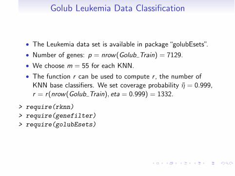
Golub Leukemia Data Classification

• The Leukemia data set is available in package“golubEsets”.

• Number of genes: p = nrow(Golub Train) = 7129.

• We choose m = 55 for each KNN.

• The function r can be used to compute r , the number ofKNN base classifiers. We set coverage probability ⌘̃ = 0.999,r = r(nrow(Golub Train), eta = 0.999) = 1332.

> require(rknn)

> require(genefilter)

> require(golubEsets)


Classification Results> options(width=40)

> golub.rnn<- rknn(data=golub.train, newdata=golub.test,

+ y=golub.train.cl, r=1332, mtry=55, seed=20081029);

> golub.rnn

Call:

rknn(data = golub.train, newdata =

golub.test, y = golub.train.cl,

r = 1332, mtry = 55, seed = 20081029)

Number of neighbors: 1

Number of knns: 1332

No. of variables used for each knn: 55

Prediction:

[1] ALL ALL ALL ALL ALL ALL ALL ALL ALL

[10] ALL ALL ALL ALL ALL ALL ALL ALL ALL

[19] ALL ALL AML AML AML AML ALL AML AML

[28] AML AML AML ALL AML AML AML


Classification Confusion Matrix

> confusion(golub.test.cl, fitted(golub.rnn))

classified as-> ALL AML

ALL 20 0

AML 2 12

Two cases are misclassified.


Variable Ranking

• A measure, called support, is defined to rank the variableimportance.

• The support of a feature is the average accuracy of the baseclassifiers containing the feature.

• The R function rknnSupport is used to compute featuresupports:


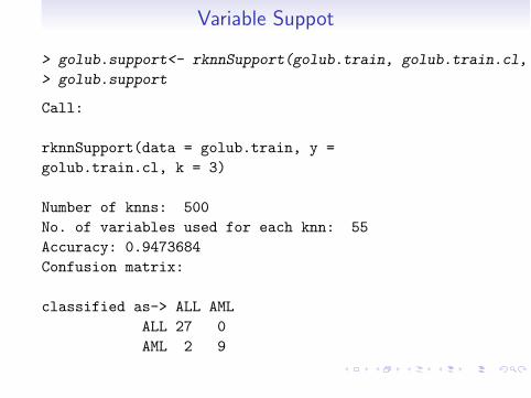
Variable Suppot

> golub.support<- rknnSupport(golub.train, golub.train.cl, k=3)

> golub.support

Call:

rknnSupport(data = golub.train, y =

golub.train.cl, k = 3)

Number of knns: 500

No. of variables used for each knn: 55

Accuracy: 0.9473684

Confusion matrix:


ALL 27 0

AML 2 9


Variable Support Plot

> plot(golub.support, main="Support Criterion Plot")

D50926_atU75276_s_atX99209_atX83573_atY00486_rna1_atU13666_atHG4557−HT4962_atZ49269_atM93651_atK02545_cds2_atX66401_cds1_atX05196_atJ04605_atAC002115_rna2_atS69115_atU81556_atM21186_atD63876_atM33600_f_atM21551_rna1_atL06797_s_atU69546_atU66618_atM60922_atM11722_atX17042_atHG4535−HT4940_s_atX56687_s_atU97105_atM27783_s_at

0.975 0.965 0.955 0.945

Support Criterion Plot

Support

Figure: Support plot for Golub leukemia training data


Two Stage Multi-step Variable Elimination

• Stage I: A fixed portion of the input variables are removed(e.g. 50%) at each step;

• Stage II: A fixed number of variables are removed (e.g. 1) ateach step;

• Balance between performance and speed.


Stage I

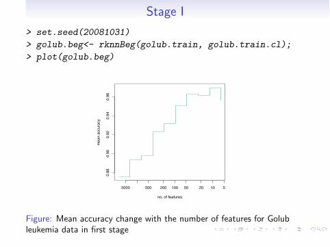
> set.seed(20081031)

> golub.beg<- rknnBeg(golub.train, golub.train.cl);

> plot(golub.beg)

2000 500 200 100 50 20 10 5

0.88

0.90

0.92

0.94

0.96

no. of features

mea

n ac

cura

cy

Figure: Mean accuracy change with the number of features for Golubleukemia data in first stage


Stage II

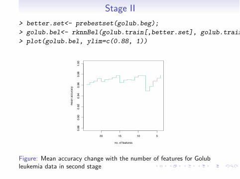
> better.set<- prebestset(golub.beg);

> golub.bel<- rknnBel(golub.train[,better.set], golub.train.cl);

> plot(golub.bel, ylim=c(0.88, 1))

20 15 10 5

0.88

0.90

0.92

0.94

0.96

0.98

1.00

no. of features

mea

n ac

cura

cy

Figure: Mean accuracy change with the number of features for Golubleukemia data in second stage


Speed Comparison with Random Forests

Random KNN approach for feature selection is faster than RandomForests:

●●

●

●●

●●●●

●●●●●●

●

●

●

●●

●

20 50 200 1000 5000 20000

12

34

5

RF time (min)

RF/

RKN

N


Stability Comparison with Random ForestsRandom KNN approach for feature selection is more stable thanRandom Forests:

Table: Average selected gene set size and standard deviation

Dataset p ⇤ c/n Mean Feature Set Size Standard Deviation

RF R1NN R3NN RF R1NN R3NN

Ramaswamy 1267 907 336 275 666 34 52Staunton 859 185 74 60 112 12 11Nutt 829 146 49 49 85 6 4Su 792 858 225 216 421 9 26NCI 688 126 187 163 118 41 33Brain 666 18 137 120 13 42 42Armstrong 468 249 76 73 1011 16 12Pomeroy 329 69 89 82 70 15 13Bhattacharjee 310 33 148 146 29 15 10Adenocarcinoma 260 8 38 11 4 20 11Golub 222 12 27 21 8 5 5Singh 206 26 25 13 32 6 6

Average 220 118 102 214 18 19


Regression

> require(chemometrics)

> data(PAC)

> x<- scale(PAC$X);

> PAC.beg<- rknnBeg(data=x, y=PAC$y, k=3, r=500, pk=0.8)

> plot(PAC.beg)

500 200 100 50 20 10 5

0.93

0.94

0.95

0.96

0.97

no. of features

mea

n ac

cura

cy

Figure: Mean accuracy change with the number of features for PAC datain second stage


Regression Performance

Random KNN can be easily extended to regression problems.

> knn.reg(x[,bestset(PAC.beg)], y=PAC$y, k=3)

$call

knn.reg(train = x[, bestset(PAC.beg)], y = PAC$y, k = 3)

$k

[1] 3

$n

[1] 209

$pred

[1] 207.6700 206.6733 206.6633

[4] 215.2267 210.3400 226.4467

[7] 226.2733 211.9933 210.0233

[10] 224.6267 219.9700 224.6933

[13] 208.4367 218.9567 223.6600

[16] 223.0000 197.0200 220.7333

[19] 250.2100 239.3733 242.2000

[22] 238.5067 220.1333 215.5533

[25] 240.2667 240.2233 234.4800

[28] 250.9567 242.6300 243.5733

[31] 242.0833 243.5667 268.2167

[34] 238.6500 244.0633 240.5433

[37] 243.5867 249.4300 253.6033

[40] 235.5333 242.6133 241.4933

[43] 268.2167 244.0133 245.6433

[46] 245.6100 223.0000 286.5367

[49] 257.9467 259.9467 271.5433

[52] 259.0833 289.9567 282.8700

[55] 287.1667 286.5933 276.0133

[58] 295.7233 239.2400 269.8300

[61] 279.1567 292.1033 290.6333

[64] 291.5200 303.6700 289.9067

[67] 285.4000 282.5600 288.4600

[70] 278.9567 283.2067 276.9267

[73] 301.7100 306.7533 302.2400

[76] 306.0133 284.1533 306.5767

[79] 282.8700 303.8233 303.6700

[82] 268.2167 281.8600 332.9800

[85] 342.8767 317.0100 323.8233

[88] 321.1333 320.9333 322.6533

[91] 366.8733 341.4433 326.3733

[94] 320.1333 323.3100 321.4233

[97] 321.6900 328.2267 323.3867

[100] 340.2033 346.4800 333.5133

[103] 320.1333 331.7133 339.3633

[106] 327.6933 337.9267 340.5300

[109] 336.9733 328.4267 338.0800

[112] 351.4067 340.9667 312.0867

[115] 336.8933 354.9367 345.7867

[118] 339.4100 349.3267 336.9733

[121] 345.7867 353.9600 383.4567

[124] 327.3967 352.1700 393.7733

[127] 388.6400 359.3100 387.1200

[130] 392.8900 371.5200 376.4767

[133] 368.1567 370.1833 349.6067

[136] 399.7667 366.0400 408.3133

[139] 403.1700 376.3500 389.7767

[142] 385.4333 416.7933 373.3967

[145] 421.6033 396.5800 401.8467

[148] 413.4600 408.3433 399.8467

[151] 399.7667 396.5800 406.5333

[154] 382.0833 411.1367 410.4533

[157] 411.7333 396.5800 379.3133

[160] 418.1600 417.0767 417.3100

[163] 421.0967 410.3700 414.9267

[166] 414.8833 418.5133 418.4167

[169] 419.5800 416.3600 421.0467

[172] 416.3667 419.6700 416.1900

[175] 418.5600 420.4167 419.9233

[178] 405.8800 415.4100 417.8067

[181] 416.5567 470.8533 404.9500

[184] 420.1267 434.0933 433.3300

[187] 442.5600 442.2867 444.2867

[190] 436.9600 454.1600 454.1900

[193] 478.4200 481.3000 465.9167

[196] 449.1900 454.9600 446.0600

[199] 469.8233 502.6000 496.0400

[202] 461.0833 477.9433 479.4600

[205] 494.0867 493.3067 496.5567

[208] 495.7000 495.6933

$residuals

[1] -10.66000000 -9.66333333

[3] -9.62333333 -15.22666667

[5] -8.87000000 -21.70666667

[7] -21.01333333 -2.29333333

[9] 5.58666667 -6.48666667

[11] -1.23000000 -4.74333333

[13] 11.93333333 2.06333333

[15] -2.62000000 0.02000000

[17] 28.95000000 9.08666667

[19] -17.51000000 -5.41333333

[21] -6.12000000 -1.94666667

[23] 16.52666667 21.86666667

[25] -2.68666667 -2.51333333

[27] 3.98000000 -12.18666667

[29] -2.38000000 -2.75333333

[31] -1.42333333 -2.84666667

[33] -26.27666667 3.78000000

[35] -0.51333333 3.02666667

[37] 1.39333333 -6.08000000

[39] -8.97333333 9.94666667

[41] 3.87666667 8.02666667

[43] -17.36666667 7.27666667

[45] 9.06666667 9.20000000

[47] 32.48000000 -29.36666667

[49] 1.28333333 3.36333333

[51] -6.30333333 6.81666667

[53] -22.68666667 -14.70000000

[55] -17.49666667 -15.20333333

[57] -4.14333333 -23.34333333

[59] 33.33000000 4.76000000

[61] 0.15333333 -11.62333333

[63] -5.74333333 -6.53000000

[65] -16.58000000 -2.21666667

[67] 2.81000000 6.47000000

[69] 3.57000000 15.34333333

[71] 11.58333333 18.88333333

[73] -4.50000000 -6.75333333

[75] -0.55000000 -3.79333333

[77] 20.17666667 -2.07666667

[79] 23.89000000 4.96666667

[81] 5.58000000 43.91333333

[83] 32.11000000 -17.79000000

[85] -26.50666667 1.00000000

[87] -4.36333333 -0.96333333

[89] -0.16333333 -1.08333333

[91] -44.88333333 -19.36333333

[93] -3.31333333 3.03666667

[95] 0.02000000 2.47666667

[97] 2.77000000 0.76333333

[99] 5.74333333 -10.51333333

[101] -16.47000000 -3.38333333

[103] 10.39666667 0.87666667

[105] -2.31333333 9.80666667

[107] -0.09666667 -1.30000000

[109] 2.40666667 14.02333333

[111] 5.93000000 -5.62666667

[113] 5.29333333 35.38333333

[115] 10.67666667 -6.39666667

[117] 4.51333333 11.81000000

[119] 6.16333333 21.55666667

[121] 14.12333333 6.77000000

[123] -22.07666667 36.82333333

[125] 13.93000000 -27.03333333

[127] -21.60000000 8.66000000

[129] -18.45000000 -23.50000000

[131] -1.98000000 -6.32666667

[133] 2.70333333 3.36666667

[135] 24.18333333 -18.20666667

[137] 15.81000000 -26.22333333

[139] -17.82000000 9.99000000

[141] -3.41666667 0.97666667

[143] -28.41333333 15.86333333

[145] -32.00333333 -5.19000000

[147] -9.34666667 -17.08000000

[149] -11.80333333 -1.34666667

[151] -1.02666667 3.42000000

[153] -6.53333333 19.72666667

[155] -5.78666667 -3.91333333

[157] -4.83333333 11.72000000

[159] 30.80666667 -5.44000000

[161] -3.29666667 -2.94000000

[163] -6.22666667 5.95000000

[165] 1.57333333 1.74666667

[167] -1.35333333 -0.85666667

[169] -2.01000000 1.74000000

[171] -2.32666667 2.43333333

[173] -0.28000000 3.48000000

[175] 1.12000000 0.19333333

[177] 0.90666667 15.24000000

[179] 6.25000000 5.06333333

[181] 6.58333333 -47.22333333

[183] 18.96000000 7.98333333

[185] -1.77333333 3.49000000

[187] -1.64000000 -0.54666667

[189] -1.72666667 6.42000000

[191] -7.92000000 -3.99000000

[193] -27.69000000 -29.73000000

[195] -12.47666667 7.03000000

[197] 6.76000000 22.38000000

[199] 2.98666667 -20.73000000

[201] -9.23000000 27.09666667

[203] 17.06666667 15.99000000

[205] 3.57333333 6.69333333

[207] 4.76333333 8.19000000

[209] 8.21666667

$PRESS

[1] 41118.98

$R2Pred

[1] 0.9696939

attr(,"class")

[1] "knnRegCV"


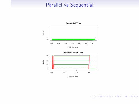
Parallel vs Sequential

> require(snow)

> require(parallel)

> sequential_time<- snow::snow.time(golub.srknn<- rknn(data=golub.train, newdata=golub.test, y=golub.train.cl, r=10000, mtry=55, seed=20081029))

> confusion(golub.test.cl, golub.srknn$pred)


ALL 20 0

AML 2 12

> cluster<- parallel::makeCluster(detectCores()-1);

> parallel_time<- snow::snow.time(golub.prknn<- rknn(data=golub.train, newdata=golub.test, y=golub.train.cl, r=10000, mtry=55, seed=20081029, cluster=cluster))

> confusion(golub.test.cl, golub.prknn$pred)


ALL 20 0

AML 2 12

> stopCluster(cluster)


Parallel vs Sequential

0.0 0.5 1.0 1.5 2.0 2.5 3.0

Elapsed Time

Nod

e

0

Sequential Time

0.0 0.5 1.0 1.5

Elapsed Time

Nod

e

01

23

Parallel Cluster Time


Extensions

1. How do we estimate entropy of complex molecules, e.g.,proteins? Combine Approximate KNN with Random KNN?

2. How do we estimate a gene interaction network? Combine theDempster-Shafer induction network algorithm with RandomKNN?

Documents

Random KNN - West Virginia Universityjharner/courses/stat623/ICDM2014.pdf · • New Modeling Methods ... >golub.bel