Embed Size (px)
Citation preview
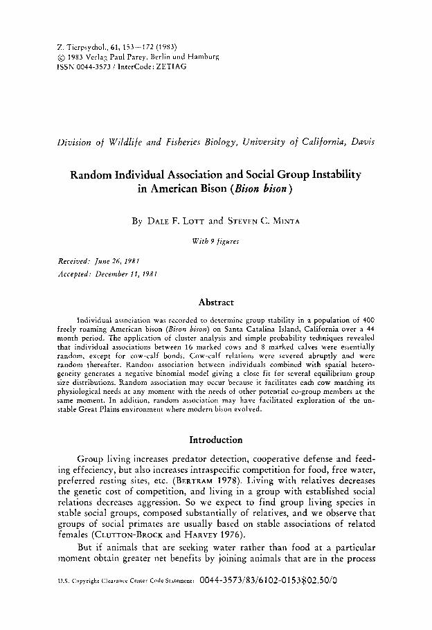
%. TierpLychol., 61, 153-172 (1983) @ 1983 Verb:; Paul Parey, Berlin und Hamburg ISSN 0044-3573 / IntcrCode: ZETIAG
Vivision of Wildlife and Fisheries Biology, University of California, Davis
Random Individual Association and Social Group Instability in American Bison (Bison bison)
By DALE F. LOTT and STEVEN C. MINTA
With 9 figures
Received: June 26, 1981
Accepted: December 11, 1981
Abstract
Individual association was recordcd to determine group stability in a population of 400 freely roaming American bison (Bison bison) on Santa Catalina Island, California over a 4 4 month period. The application of cluster analysis and simple probability techniques revcaled that individual associations between 16 marked cows and 8 marked calves were essentially random, except for cow-calf bonds. Cow-calf relations were severed abruptly and were random thereafter. Random association between individuals combined with spatial hetero- geneity generates a negative binomial model giving a close fit for several equilibrium group size distributions. Random association may occur because it facilitates each cow matching its physiological needs a t any moment with the needs of other potential co-group members a t the same moment. I n addition, random association may have facilitated exploration of the un- stable Great Plains environment where modern bison evolved.
Introduction
Group living increases predator detection, cooperative defense and feed- ing effeciency, but also increases intraspecific competition for food, free water, preferred resting sites, etc. (BERTRAM 1978). Living with relatives decreases the genetic cost of competition, and living in a group with established social relations decreases aggression. So we expect to find group living species in stable social groups, composed substantially of relatives, and we observe that groups of social primates are usually based on stable associations of related females (CLUTTON-BROCK and HARVEY 1976).
But if animals that are seeking water rather than food a t a particular moment obtain greater net benefits by joining animals that are in the process
US. Copyright Clearance Center Code Statement: 0044-3573/83/6102-0153$02.50/0
154 DALE F. LOTT and STEVEN C. MINTA
of satisfying the same needs rather than by staying with kin or familiar con- specifics as co-group members, there is selection pressure acting against group stability. Unstable groups have been observed in female pronghorn (KITCHEN 1974). Thus both kinds of social organization are realized in nature, raising the question of the conditions under which each is favored.
Female American bison spend their lives in groups composed of other females and immature males. SETON (1929) and SOPER (1941) believed that these were stable groups composed of relatives. MCHUGH (1958) doubted that there were any stable associations beyond cow and calf. FULLER (1960) pro- posed that there might be stable groups of 11-20 but considered his data inconclusive. MEAGHER (1973) thought her evidence for strong loyalty to home ranges suggested some sort of stable group structure. VAN VUREN (1978) con- cluded that stable social groups would have to be 10 individuals or less and might not exist at all.
We found no significant deviation from randomness in the individual associations of adult females on Catalina Island. In fact, once the period of nearly continuous association between cow and calf ended, the association of that dyad became essentially random.
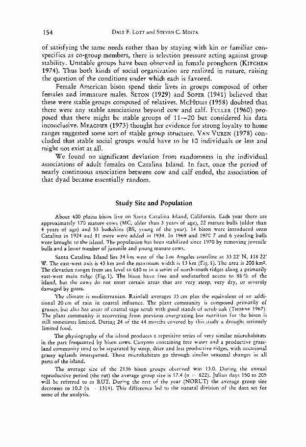
Study Site and Population
About 400 plains bison live on Santa Catalina Island, California. Each year there are approximately 170 mature cows (MC, older than 3 years of age), 22 mature bulls (older than 4 years of age) and 55 budrskins (BS, young of the year). 14 bison were introduced onto Catalina in 1924 and 1 1 more were added in 1934. In 1969 and 1970 7 and 6 yearling bulls were brought to the island. The population has been stabilized since 1970 by removing juvenile bulls and a lesser number of juvenile and young mature cows.
Santa Catalina Island lies 34 km west of the Los Angeles coastline at 33 2 2 ' N , 118 22' W. The east-west axis is 43 km and the maximum width is 13 km (Fig. 1). The area is 200 km*. The elevation ranges from sea level to 610 m in a series of north-south ridges along a primarily east-west main ridge (Fig. 1). The bison have free and undisturbed access to 86 9'0 of the island, but the cows do not enter certain areas that are very steep, very dry, or severely damaged by goats.
The climate is mediterranian. Rainfall averages 33 cm plus the equivalent of an addi- tional 20 cm of rain in coastal influence. The plant community is composed primarily of grasses, bur also has arcas of coastal sage scrub with good stands of scrub oak (THORNE 1967). The plant community is recovering from previous overgrazing but nutrition for the bison is still sometimes limited. During 24 of the 44 months covered by this study a drought seriously limited food.
The physiography of the island produces a rcpetitive series of very similar microhabitats in the part frequented by bison cows. Canyons containing free water and a productive grass- land community tend to be separated by steep, drier and less productive ridges, with occasional grassy uplands interspersed. These microhabitats go through similar seasonal changes in all parts of the island.
The average size of the 2136 bison groups observed was 13.0. During the annual reproductive period (the rut) the average group size is 17.4 (n = 822). Julian days 150 to 205 will be referred to as RUT. During the rest of the year (NORUT) the average group size decreases to 10.2 (11 = 1314). This difference led to the natural division of the data set for some of the analysis.
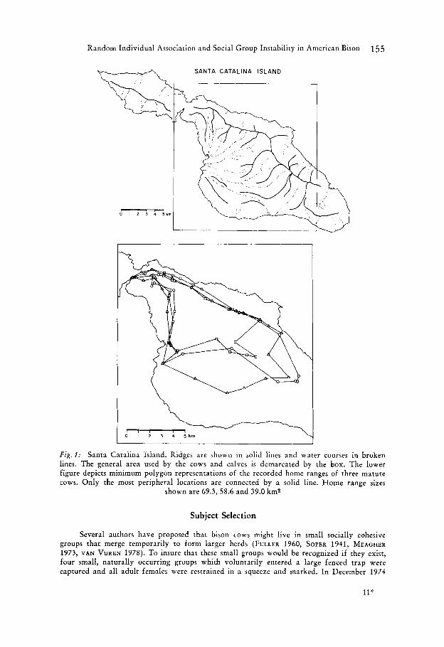
Random Individual Association and Social Group Instability in American Bison 155
- 1 0 I 2 3 4 S k m
Fig. 1 : Santa Catalina Island. Ridges are shown in solid lines and water courses in broken lines. The general area used by the cows and calves is demarcated by the box. The lower figure depicts minimum polygon representations of the recorded home ranges of three mature cows. Only the most peripheral locations are connected by a solid line. Home range sizes
shown are 69.3, 58.6 and 39.0 km2
Subject Selection
Several authors have proposed that bison cows might live in small socially cohesive groups that merge temporarily to form larger herds (FULLER 1960, SOPER 1941, MEAGHER 1973, VAN VUREN 1978). To insure that these small groups would be recognized if they exist, four small, naturally occurring groups which voluntarily entered a large fenced trap were captured and all adult females were restrained in a squeeze and marked. In December 1974
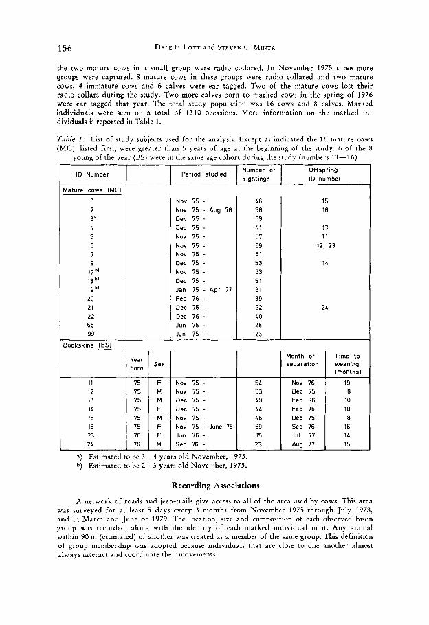
156 DALE F. LOTT and STEVEN C. MINTA
Number of sightings
ID Number Period studied Offspring ID number
4ature cows (MC)
0 2
L 5 6 I 9
17 b’
3 4
18 bl
19 b’
20 21 22 66 99
3uckskins (BSI I
F Jun 16 - M Sep 76 -
11 15 12 15 13 15 14 15 15 15 16 75 23 16 24 76
Jut I1 35 23 Aug I1
NOV 15 - NOV 15 - Aug 1 6 Dec 1 5 - Dec 75 - NOV 15 - NOV 15 - NOV 15 - Dec 15 -
Dec 15 - Jan 15 - Apr I1 Feb 1 6 - Dec 15 - Dec 15 - Jun 15 - Jun 15 -
NOV 75 -
46 56 69 L1 51 59 61 53 6 3 51 31 39 52 LO 28 23
Nov 15 -
Dec 15 - Dec 15 -
Nov 15 - June I8
NOV 75 -
NOV 15 -
54 53 49 LL 48 69
15 16
13 11
12, 23
14
24
Month of separation
Nov 16 Dec 15 Feb 16 Feb 76 Dec 75 Sep 16
Time to weaning (months1
19 8
10 10 8
16 I L 15
Recording Associations
A network of roads and jeep-trails give access to all of the area used by cows. This area was surveyed for at least 5 days every 3 months from November 1975 through July 1978, and in March and June of 1979. The location, size and composition of each observed bison group was recorded, along with the identity of each marked individual in it. Any animal within 90 m (estimated) of another was treated as a member of the same group. This definition of group membership was adopted because individuals that are close to one another almost always interact and coordinate their movements.
Random Individual Association and Social Group Instability in American Bison 157
Data Analysis
To learn if particular cows spent all o r most of their time with certain other cows or if they associated more or less randomly, we analysed the degree of association between marked cows. T w o known cows in the same group is an instance of association. One being present and the other absent was an instance of non-association.
The first identification of each individual during a 24-h interval was used in the analysis. Since not all individuals were marked throughout the study period, only the period
during which both members of a dyad were identified was analysed. We examined the possibility of changes in association during the study by generating a printout of the sighting of each individual with every other. Except for cows and their calves, the degree of association did not change. The cow-calf separation was abrupt and permanent, which allowed us easily to examine associations with and without the influence of the cow-calf bond. Pre-separation association was analyzed using all data except that of the 6 calves after separation from their mothers. Post-separation analysis used all data except that of the calves prior to separaxion from their mothers. Consequently we first examined the entire da ta set as i f associations were stable, then divided the data set into pre- and post-separation subsets by adjusting for separa- tion effects on association of all individuals.
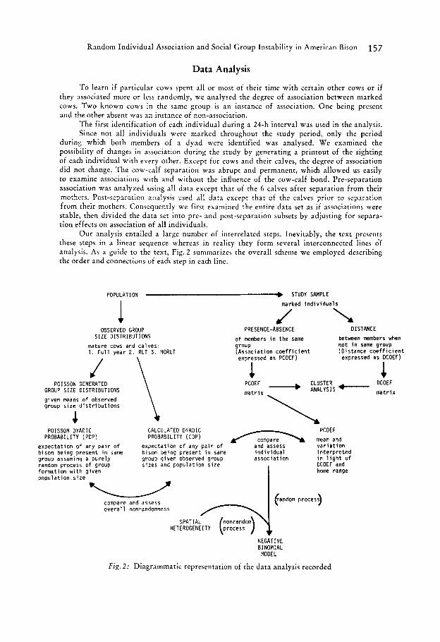
Our analysis entailed a large number of interrelated steps. Inevitably, the text presents these steps in a linear sequence whereas in reality they form several interconnected lines df analysis. As a guide to the text, Fig. 2 summarizes the overall scheme we employed describing the order and connections of each step in each line.
POPULATION + STUDY SAMPLE
1 OBSERVED GROUP
S I Z E DISTRIBUTIONS
mature cows and ca lves: 1 . F u l l year 2 . RUT 3 . NORUT
POISSON GENERATED GROUP S I Z E DISTRIBUTIONS \
\ given means of observed group s i z e d i s t r i b u t i o n s
marked i n d i v i d u a l s
J PRESENCE-ABSENCE DISTANCE
of members i n the same between members when group n o t i n same group (Assoc ia t i on c o e f f i c i e n t (Dis tance c o e f f i c i e n t
expressed as DCOEF) expressed as PCOEF)
1 1
POISSON DYADIC CALCULATED D Y A D I C PCOEF mean and v a r i a t i o n
DCOEF and
PROBABILITY (POP) PROBABILITY (COP)
expec ta t i on of any p a i r o f b i son being present i n same b ison being present i n same i n d i v i d u a l i n t e r p r e t e d group assuming a p u r e l y group g iven observed group assoc ia t i on i n l i g h t o f random process of group format ion w i t h g iven home range popu la t i on s i z e
expec ta t i on of any p a i r of
s izes and popu la t i on s i z e
and assess
compare and assess o v e r a l l nonrandomness
SPATIAL
NEGATIVE BINOMIAL MODEL
F i g . 2: Diagrammatic representation of the da ta analysis recorded
158 DALE F. LOTT and STEVEN C. MINTA
Development of Association Coefficient
Presence-absence data was analysed in a two by two contingency table for each dyad, and the resulting index of association was expressed as the probability coefficient (PCOEF). The PCOEF is derived from standard probabilities of a two by two contingency table where n,, is the number of co-occurrences of A and B, n12 the number of occurrences of A wi,thout B, nZ1 is the number of occurrences of B without A, and n22 is the number of times neither A nor B occurred. The total number of occurrences is N = nll + nI2 + nZ1 + n22. From these
n.1 n . numbers the following probabili,tiescan be estimated: p(AB) = k, p(A) = 2, p(B) = -
N N N As these probabilities are stated, their computation appears to require N. But the
following analysis demonstrates that the PCOEF does not require nZ2 (the number of times the sample space was sampled when neither A nor B was observed) and therefore does not require N. If a pair of individuals are randomly associating, then they are occurring in groups independently of each other. In that case the following relation should hold P(AB) = P(A)P(B) which creates the possibility of the following ratio:
P(AB) W W B )
When A and B are associating independently this ratio will be unity. We can normalize this ratio by taking the square root of the denominator such that
"11
N
Notice that the Ns have cancelled out of the resulting formula. Consequently the PCOEF does not rely on knowledge of N, the total times the sample space was randomly sampled for A and B.
In fact, the PCOEF is invariant with respect to N and becomes an unconditional estimator of P(AB) assuming the sample space was randomly searched (not randomly sampled; MINTA in prep.) for A and B and the sampling in te rn1 was long enough for thorough population mixing. When the ratio has been normalized 0 signifies no chance of A and B co-occurring while 1 signifies certainty of co-occurrence.
Relationship of PCOEF to other Coefficients of Association
Under certain circumstances the PCOEF may become identical with other coefficients of association. Given a random search we can assume that binomial A and B have an equal probability of being sampled. Therefore, by the central limit theorem, and n,. will vary normally around a common mean with the variance being inversely proportional to the
n.* + nl. sample size. For large sample sizes then it might be proper to allow
2
(DICE In that case the PCOEF becomes Dice's coefficient of coincidence which is
1945). Alternatively, the probability of sampling A (ml) may be made equal to the probability of sampling B (nl.) by establishing a sampling regime that assures equality or by having the sample size approach infinity. As the sampling size becomes larger and nl. converge with
a variance approaching 0. In either case PCOEF reduces to Simpson's coefficient, simply "11 (SIMPSON 1943). Neither of these coefficients, however, should be applied to our data. When sample size is low or moderate, the search for A and B is random, and P(AB) has a small value then the PCOEF should be used.
= nl. =
2% + nl .
n , .
R.indom Individual Association and Social Group Instability in American Bison 159
Results of Association Analysis
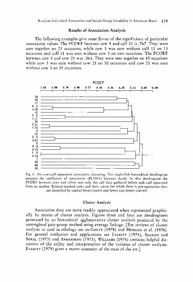
The following examples give some flavor of the significance of particular association values. The PCOEF between cow 5 and calf 11 is .767. They were seen together on 23 occasions, while cow 5 was seen without calf 11 on 13 occasions and calf 11 was seen without cow 5 on two occasions. The PCOEF between cow 3 and cow 21 was .263. They were seen together on 15 occasions while cow 3 was seen without cow 21 on 50 occasions and cow 21 was seen without cow 3 on 35 occasions.
PCOEF 1.00 0.89 0.78 0.68 0.57 0.46 0.35 0.25 0.14 0.03 -0.08
18 19 17
A 2 a 16
12 c 5 c 11
20 F 21 f 24
3 15
Q 6 d 23
0 B 4 b 13 E 9 e 14
7 22 66 99
I, ' I
I 1
Fig . 3: Pre cow-calf separation association clustering. This single-link hierarchical dendrogram presents the coefficient of association (PCOEF) between dyads. In this dendrogram the PCOEF between cows and calves uses only the calf da ta gathered before each calf separated from its mother. Related marked cows and their calves for which there is pre-separation data
are identified by capital letters (cows) and lower case letters (calves)
Cluster Analysis
Association data are more readily appreciated when represented graphic- ally by means of cluster analysis. Figures three and four are dendrograms generated by an hierarchical agglomerative cluster analysis produced by the unweighted pair-group method using average linkage. [For reviews of cluster analysis as used in ethology see DE GHETT (1978) and MORGAN et al. (1976). For general mechanics and applications see EVERITT (1974), SNEATH and SOKAL (1973) and ANDERBERG (1 973). WILLIAMS (1976) contains helpful dis- cussion of the utility and interpretation of the varieties of cluster analyses. EVERITT (1979) gives a recent summary of the state of the art.].
160 DALE F. LOTT and STEVEN C. MINTA
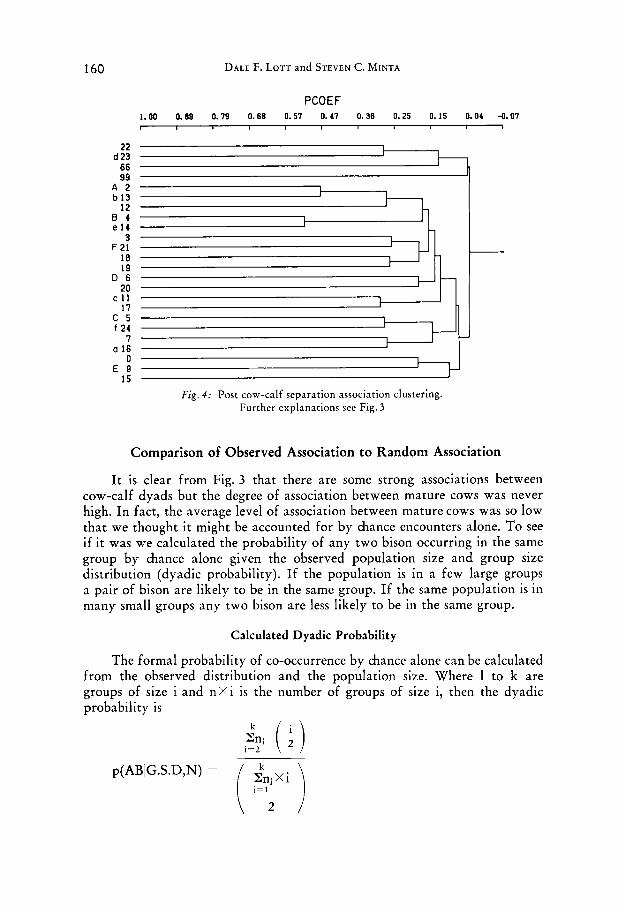
PCOEF 1.00 0.89 0.79 0.68 0 . 5 1 0.47 0.36 0.25 0.15 0.04 -0.07
A 2 b 13
12 0 4 e 14
3 F 21 18 19
D 6 2 0
c 11 17
c 5 f 24
7 a 16
0 € 9
15
Fig. 4 : Post cow-calf separation association clustering. Further explanations see Fig. 3
Comparison of Observed Association to Random Association
It is clear from Fig. 3 that there are some strong associations between cow-calf dyads but the degree of association between mature cows was never high. In fact, the average level of association between mature cows was so low that we thought it might be accounted for by chance encounters alone. To see if it was we calculated the probability of any two bison occurring in the same group by chance alone given the observed population size and group size distribution (dyadic probability). If the population is in a few large groups a pair of bison are likely to be in the same group. If the same population is in many small groups any two bison are less likely to be in the same group.
Calculated Dyadic Probability
The formal probability of co-occurrence by chance alone can be calculated from the observed distribution and the population size. Where 1 to k are groups of size i and n x i is the number of groups of size i, then the dyadic probability is
Random Individual Association and Social Group Instability in American Bison 161
which is the expected probability of any two bison associating under the con- straints of a given population size and group size distribution.
Recall that the PCOEF is a sample estimate of a particular dyad from a sampled set of the population. I t is estimating the probability of those two animals being found in the same group. Given enough PCOEF’s, and assuming that the sampled PCOEF’s are a random, unbiased sample of the population, we may estimate the mean and variation of PCOEF’s and compare them with the calculated dyadic probability (CDP).
This comparison is important because the C D P has only two constraints (population size and group size) while the PCOEF has all the constraints of the actual animal. We can estimate the magnitude of the effects of the addi- tional constraints by comparing the CDP and the mean PCOEF. The variation of the PCOEF may tell us whether individuals in the population are behaving uniformly or if one segment is being highly aggregative and another very solitary.
CDP Compared to PCOEF
The mean PCOEF for the sampled M C f B S is . lo3 (s=.107, n=275) and the CDP for the population of M C f B S is .104. (For the sampled 16 M C by themselves the mean PCOEF is .084 (s = .069, n = 120) compared to a C D P of .096.) The PCOEF closely estimates the CDP.
This estimate of the chance expectation of a dyad treats bison as objects in a common space governed only by group size and population size. In fact, bison are also constrained by home range size, home range overlap and rate of movement through the home range among other factors. In fact, the home ranges of the 16 sampled MC vary in the overlap from 60 to 100%. This incomplete overlap may result in a pair of bison having fewer chances to associate.
From an analysis of their home range patterns (LOTT and MINTA, in prep.) our impression is that this spatial constraint would contribute to a slight underestimation of the CDP by the PCOEF in cases of low home range overlap. O n the other hand the PCOEF may overestimate the CDP when a pair has high overlap in small home ranges. T w o bison being confined by their home ranges to common partial region of the island may have increased fre- quency of contact relative to the whole population. This raises the possibility that the extreme closeness of the PCOEF and the CDP may be due less to refined accuracy of estimation than to the approximate equilibrium produced by compensating over and under estimates.
Relationship between Home Ranges and Associations
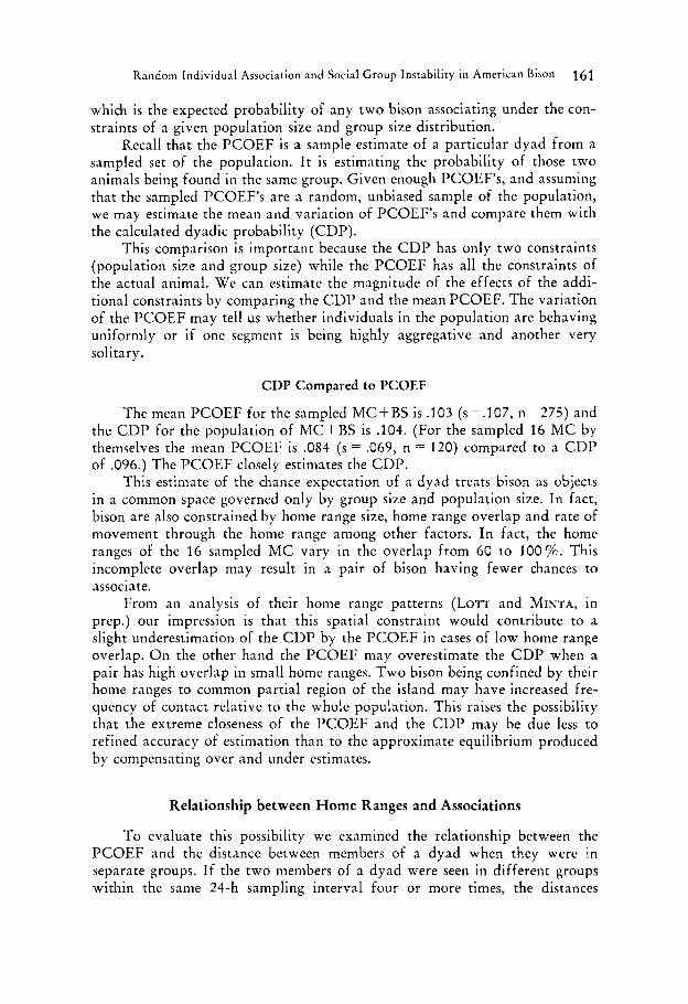
T o evaluate this possibility we examined the relationship between the PCOEF and the distance between members of a dyad when they were in separate groups. If the two members of a dyad were seen in different groups within the same 24-h sampling interval four or more times, the distances
162 DALE F. LOTT and STEVEN C. MINTA
between them were averaged. This was accomplished by first recording group locations on a grid system 500 foot (152 m) squares that was overlayed on 15-min topographic maps. A Cartesian coordinate system assigned coordinates to each square so distances between groups could be calculated. Since the center
50
40 >
30 W 3 0 !$ 20 LL
10
DCOEF DISTANCE
( m )
r (421
- r ( 3 )
( I ) ( I1
285 80 75 70 65 60 55 50 45 40 35 30 25 20 15 10 0 I
t -
- r ( 3 )
( I ) ( I1
285 80 75 70 65 60 55 50 45 40 35 30 25 20 15 10 0 I
Fig . J: Frequency distribution of distance coefficients (DCOEF). Number of cases in each DCOEF interval are in parentheses
0 f 24
€ 9 I
15 12
d 23 99
B 4 a 16
18 F 21
17 19
e 1 4 A 2
20 c 11
3 b 13 c 5
22 D 6
66
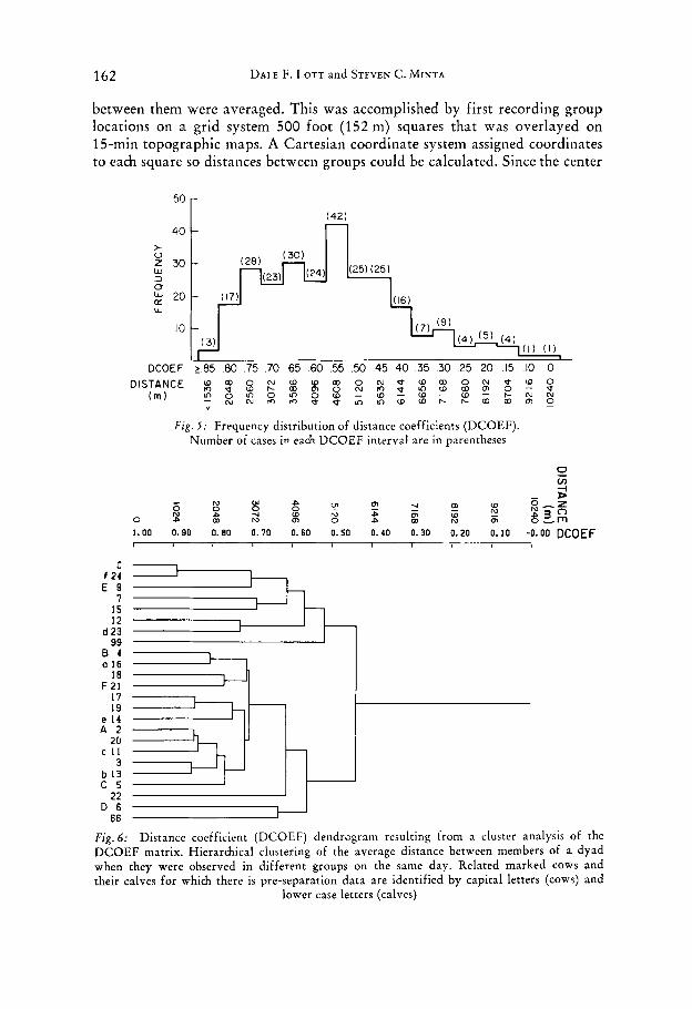
1.00 0.90 0.80 0.70 0.60 0.50 0.40 0.30 0.20 0.10 -0.00 DCOEF I
Fig. 6: Distance coefficient (DCOEF) dendrogram resulting from a cluster analysis of the DCOEF matrix. Hierarchical clustering of the average distance between members of a dyad when they were observed in different groups on the same day. Related marked cows and their calves for which there is pre-separation data are identified by capital letters (cows) and
lower case letters (calves)
Random Individual Association and Social Group Instability in American Bison 163
of each square was used in measurements, the maximum calculation error of the distance between two groups in two different squares was 152 m. The mean distance between marked bison was 4250 m (range = 91-10 240 m). The distances are approximately normally distributed around the mean (when a square root transformation is applied, kurtosis and skewness are close to 0, see Fig. 5). Fig. 6 is the result of a cluster analysis on the mean dyadic distan- ces for the entire study.
Index of Home Range Overlap
Our sampling design did not lend itself to a “nearest neighbor” type of analysis (after CLARK and EVANS 1954). Therefore, in order to relate the distances to the PCOEF we transformed the dyadic distances into a com- parable coefficient. The averaged dyadic distances were normalized to produce a distance coefficient (DCOEF) for each dyad with values ranging between O and 1:
mean distance dyadi max. single distance of any dyad
Consequently a DCOEF near 1 means a pair of bison keep a minimal distance from each other when they are not actually in the same group and a DCOEF near 0 means a pair maintains about as much distance between themselves as any pair observed. Figure six is the dendrogram generated from the DCOEF matrix of each dyad that was seen separately on the same day on four or more days.
The Spearman correlation coefficient between the PCOEF and the DCOEF was .53 (p < .001, n = 264). This significantly positive correlation is concordant with our hypothesis that association of dyads covaries with home range overlap, and that this contributes to a biased estimation of the CDP by the PCOEF. The normal distribution of the mean dyadic distances leads us to believe that the proximity of bison to each other is random, with the exception of cow-calf relationships. The closeness of the PCOEF and the CDP leads us to conclude that bison cows are associating randomly.
DCOEF = 1-
Cow-calf Separation
The low association between cows suggests that heifers leave their mothers by the time they become adults. The duration of association between cows and their calves provides a direct test of that suggestion. 8 calves from marked mothers were tagged within 7 months of their birth. Records of the co-occur- rence of these pairs revealed the timing of the separation of 7 of them from their mothers. The four male calves separated from their mothers at 8, 8, 10 and 15 months of age. The three female calves whose date of separation is certain separated a t 10, 14 and 19 months of age. The fourth female’s mother lost her radio collar when the calf was 16 months old, making that a minimal preseparation period.
164 DALE F. LOTT and STEVEN C. MINTA
The separation was typically rather abrupt. For example, a heifer was with her mother 35 of the 37 times she was seen during the first 19 months of her life, but was seen with her only 3 of the 28 times she was observed during the next 16 months. We evaluated cow-calf separation by hypothesizing that non-related M C and BS should have the same average level of association as related M C and BS after separation. Using the post-separation data set, the 120 non-related MC and BS dyad combinations gave a mean PCOEF of .088. The seven related MC and BS have a mean of .115. The distribution shape (similar to Fig. 7) prompted us to use a Mann-Whitney test which was sig- nificant at .17. We cannot reject our hypothesis a t an alpha of .05. This in- dicates little if any residual tendency to associate with the mother. Figs. 3 and 4 compare the PCOEFs of calves and their mothers pre- and post- separation.
Group Membership Randomly Generated
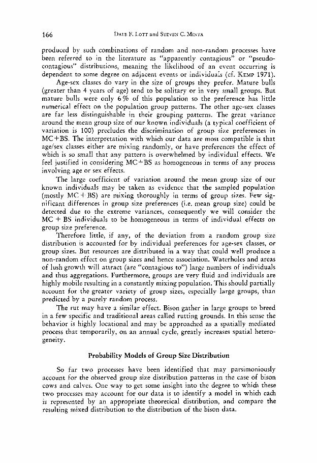
The demonstration that associations among individuals are essentially random raises the possibility that group membership is generated by a random process. We can evaluate this possibility by comparing a distribution of group sizes that were observed with the accompanying distribution produced by a random (Poisson) process. This was accomplished by taking the mean of the observed group size distribution and generating its accompanying theoretical distribution as a truncated Poisson process (cf. COHEN 1971). The Poisson distribution is truncated at zero since a group must be at least of size one. We then computed the dyadic probability that would be expected given the Poisson generated group size distribution (PDP) and compared it to the CDP.
If CDP = PDP then the observed groups are falling in a random in- dependent pattern around the mean group size of the distribution. If the CDP > PDP then there is aggregation. In the Poisson distribution the mean and variance are equal. If the variance of the observed distribution is greater than the mean the sample is overdispersed or aggregated. If the variance is less than the mean the sample is underdispersed or segregated. In our observed distributions the variance/mean ratio for the entire population ranges from 14.1 during the NORUT to 33.2 during the RUT. For just those bison groups containing mature cows (MC) the variance/mean ratio is 12.5 NORUT and 32.1 RUT. These ratios show that bison aggregate, especially during the rut.
The CDP : PDP ratio tells us exactly how much this aggregation increases the probability of association for any dyad compared to random association. For the entire population rhis ranges from 2.2 in the NORUT to 2.8 in the RUT. The CDP:PDP for mature cows and buckskins (MC+BS) in the groups of which they are part is similar: 2.0 to 2.7. When a chi square goodness-of-fit test is applied to the observed distributions compared to the truncated Poisson distributions, the minimum chi square value is more than 1000.
The J-shaped distribution of the PCOEF values (Fig. 7) is quite similar to that of the distribution of group sizes leading to the CDP values during
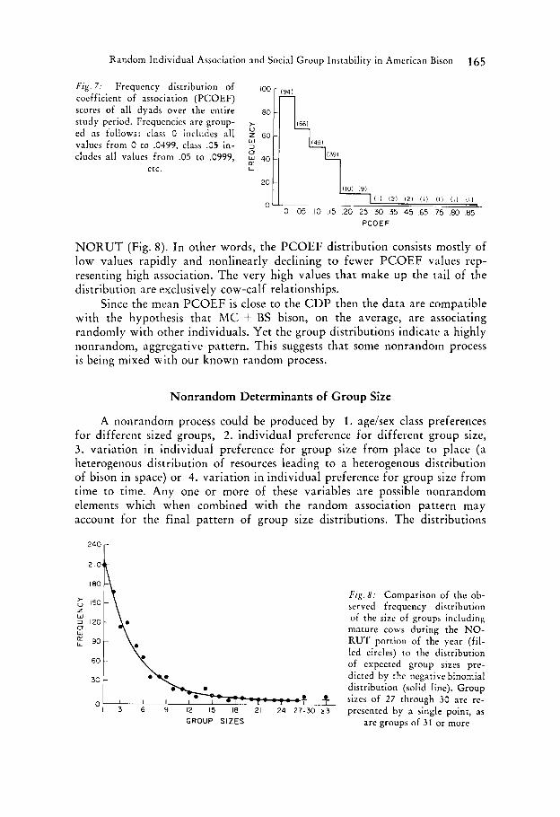
Random Individual Association and Social Group Instability in American Bison 165
F i g . 7: Frequency distribution of coefficient of association (PCOEF)
ed as follows: class 0 includes all
scores of al l dyads over the entire study period. Frequencies are group-
values from 0 to .0499, class .05 in- cludes all values from .05 to .0999,
60
40 0
etc. LL
I l l I21 I21 (0 1 1 1 I l l I l l
0 0 ~ ~ ~ 0 25 30 35 45 65 75 80 85 0
PCOEF
N O K U T (Fig. 8). In other words, the PCOEF distribution consists mostly of low values rapidly and nonlinearly declining to fewer PCOEF values rep- resenting high association. The very high values that make up the tail of the distribution are exclusively cow-calf relationships.
Since the mean PCOEF is close to the CDP then the data are compatible with the hypothesis that h4C + BS bison, on the average, are associating randomly with other individuals. Yet the group distributions indicate a highly nonrandom, aggregative pattern. This suggests that some nonrandom process is being mixed with our known random process.
Nonrandom Determinants of Group Size
A nonrandom process could be produced by 1. age/sex class preferences for different sized groups, 2. individual preference for different group size, 3. variation in individual preference for group size from place to place (a heterogenous distribution of resources leading to a heterogenous distribution of bison in space) or 4. variation in individual preference for group size from time to time. Any one or more of these variables are possible nonrandom elements which when combined with the random association pattern may account for the final pattern of group size distributions. The distributions
F i g . 8 : Comparison of the ob- served frequency distribution of the size of groups including mature cows during the NO- RUT portion of the year (fil- led circles) to the distribution of expected group sizes prc- dictcd by the ncgative binomial distribution (solid line). Group
7 f sizes of 27 through 30 arc rc- -30 231 presented by a single point, as
GROUP SIZES are groups of 3 1 or more
166 DALE F. LOTT and STEVEN C. MINTA
produced by such combinations of random .and non-random processes have been referred to in the literature as “apparently contagious” or “pseudo- contagious” distributions, meaning the likelihood of an event occurring is dependent to some degree on adjacent events or individuals (cf. KEMP 1971).
Age-sex classes do vary in the size of groups they prefer. Mature bulls (greater than 4 years of age) tend to be solitary or in very small groups. But mature bulls were only 6 % of this population so the preference has little numerical effect on the population group patterns. The other age-sex classes are far less distinguishable in their grouping patterns. The great variance around the mean group size of our known individuals (a typical coefficient of variation is 100) precludes the discrimination of group size preferences in MCfBS. The interpretation with which our data are most compatible is that age/sex classes either are mixing randomly, or have preferences the effect of which is so small that any pattern is overwhelmed by individual effects. We feel justified in considering MC+BS as homogeneous in terms of any process involving age or sex effects.
The large coefficient of variation around the mean group size of our known individuals may be taken as evidence that the sampled population (mostly MC + BS) are mixing thoroughly in terms of group sizes. Few sig- nificant differences in group size preferences (i.e. mean group size) could be detected due to the extreme variances, consequently we will consider the MC + BS individuals to be homogeneous in terms of individual effects on group size preference.
Therefore little, if any, of the deviation from a random group size distribution is accounted for by individual preferences for age-sex classes, o r group sizes. But resources are distributed in a way that could well produce a non-random effect on group sizes and hence association. Waterholes and areas of lush growth will attract (are “contagious to”) large numbers of individuals and thus aggregations. Furthermore, groups are very fluid and individuals are highly mobile resulting in a constantly mixing population. This should partially account for the greater variety of group sizes, especially large groups, than predicted by a purely random process.
The rut may have a similar effect. Bison gather in large groups to breed in a few specific and traditional areas called rutting grounds. In this sense the behavior is highly locational and may be approached as a spatially mediated process that temporarily, on an annual cycle, greatly increases spatial hetero- geneity.
Probability Models of Group Size Distribution
So far two processes have been identified that may parsimoniously account for the observed group size distribution patterns in the case of bison cows and calves. One way to get some insight into the degree to which these two processes may account for our data is to identify a model in which each is represented by an appropriate theoretical distribution, and compare the resulting mixed distribution to the distribution of the bison data.
Random Individual Association and Social Group Instability in American Bison 167
Many models generated by mixing probabilistic distributions have inferen- tial and explanatory value. But most such models fail, or produce superficial description, either because there are too many processes or because the pro- cesses cannot be identified or are hard to differentiate. Even after two or more processes have been properly identified it is still necessary to 1. ascertain the nature of each process, 3 . avoid or minimize violations of assumptions. If these things are not accomplished then most often one cannot know how to derive the model since one model may have a multiplicity of derivations or generations.
All these requirements are adequately fulfilled by our data on the bison cows and calves. We have a simple system that, for the level of our analysis, is a moderately homogeneous and continually mixing set of subjects. One process, random individual association, has been identified and estimated and another of high explanatory value, spatial heterogeneity, has been identified. Now we can decide upon appropriate models of each of these two processes and mix them to create an inferential model in the form of a single theoretical distribution defined by two or more parameters. If there is a close f i t one may conclude that the observed distribution may be described by the theo- retical distribution. This can be an excellent source of inference about the biological phenomena if the data set is suitable and the parameters are inter- pretable in the light of biological knowledge.
2 . estimate appropriate parameters,
The Negative Binomial Model
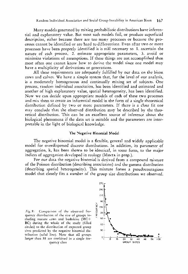
The negative binomial model is a flexible, general and widely applicable model for overdispersed discrete distributions. In addition, its parameter of aggregation, k, has been shown to be identical, in some form, to the major indices of aggregation developed in ecology (MINTA in prep.).
For our data the negative binomial is derived from a compound mixture of the Poisson distribution (describing association) and the gamma distribution (describing spatial heterogeneity). This mixture forms a pseudocontagious model that closely f i ts a number of the group size distributions we observed.
F i g . 9 : Comparison of the observed fre- quency distribution of the size of groups in- cluding mature cows and buckskins ( M C t BC) during the whole of the study (filled circles) t o the distribution of expected group sizes predicted by the negative binomial dis- tribution (solid line). Note that all groups larger than 58 are combined in a single fre-
6o
30-
quency class GROUP SIZES
168 DALE F. LOTT and STEVEN C. MINTA
The f i t is statistically reliable in M C groups in the NORUT (see Fig. 8, chi square=35.3, d.f.=27, p<.05). In the case of M C + BS during the NORUT and during the entire year the typically long tail (representing very few but very large aggregations) of the observed group size distributions precluded a significant chi-square f i t to the negative binomial distribution. However the fi t is very close (see Fig. 9). This is compatible with the explanation that the M C + BS were randomly choosing individuals (groups) in an heterogeneous sampling space. This is strong evidence that a t times these group processes are driven by random and environmental forces.
The parameter of aggregation, k, of the fitted distribution can be viewed as an index of the degree to which the spatial heterogeneity manifests itself as being “contagious” to individuals (and thus groups) outside the RUT. In the case of MC during NORUT, k = .8. For M C during the whole year k = .6. For MC + BS for the whole year, k = .5. In contrast there is such a marked contagion” operating during the RUT that the negative binomial does not
f i t the greatly overdispersed distributions observed. The closest fits for the R U T group distributions gave a k close to 0 indicating extreme aggregation
There are other distributions that will f i t overdispersion too great for the gamma distribution. PATIL et al. (1968) classify over 70 such mixed distribu- tions. Hence it is possible that some distributional replacement for the gamma may describe the spatial heterogeneity at all times or an additional process may be involved during the RUT. For a discussion of mixed distribution models and model fitting see ORD (1972), JOHNSON and KOTZ (1969), and COLEMAN (1964).
“
Discussion
Effect of Environmental Funneling on Random Association
It is clear that stable associations between cows are not characteristic of at least this population of bison. The close fit of our data to the compound discrete probability model suggests that co-group membership may be adequa- tely explained by the action of environmental funneling on animals that associate randomly. We envision three major categories of funneling: topo- graphic, phenological and reproductive. Steep slopes are less accessible to bison than flat areas. Bison aggregate at sources of free water. The distribution of plant communities and their phenological patterns influence where and when bison cluster. Bison also aggregate during the rut.
We may view natal dispersal as a single ontogenetic phenomenon occurring when the parent-offspring bond is severed (BAKER 1978). Dispersal, however, is almost always “away from something or someplace” or “to something or someplace”. I t can be viewed as a centripetal biological process (parent-off- spring attachment) being replaced by a centrifugal process (TAYLOR and TAYLOR 1977). A disperser may move away from its origin to find a mate or to establish a home range. An animal that is social may disperse to another group. An animal may be forced to disperse under the pressure of aggression.
Random Individual Association and Social Group Instability in American Bison 169
I n the Santa Catalina bison the cessation of a cow-calf bond seems to be replaced by a random process in the sense of association.
The absolute value of the indices of association observed on Catalina are probably raised by the spatial limitations of the island and the total size of the population, but the association values appear to be increased as much be- tween mature cows as between cows and their calves post-separation, and to be random in both cases.
Functional Analysis of Random Association
A random pattern of association randomly arrived a t does not seem a strong candidate for a functional analysis. I t seems simplest to aisume that a lack of advantage in stable associations leads to a lack of tendency for intra- individual affinity between mature cows rather than to look for advantage in a pattern of behavior that actively produces random association.
But the abruptness of the cow and calf separation contradicts this inter- pretation. Bison calves are generally weaned by about 6 months of age so the calves we observed stayed with their mothers for some time after they had stopped nursing; in some cases for several months afterward. We do not know what function, if any, this behavior pattern serves, but given that it occurs one would expect some matriarchial group formation to occur if nothing intervened. The fact that it does not occur suggests that the bond between mother and female calf is actively disrupted by some process in the service of promoting a more flexible social organization.
The question then becomes, what are the positive values of lack of associa- tion? One possibility is the advantage inherent in the ability to make a partic- ularly good match between the physiological needs of the individual a t any one moment and the needs of other members of the particular group it is in, or can join, a t that moment. For example, an individual with an especially high food need might break off feeding and go to water when the rest of its group does. After watering the group would normally rest a t the water hole for several hours. But if a group that had arrived earlier left to resume grazing the hungry individual has the alternatives of remaining with his group and continuing to rest or separating from his group and resuming a higher priority activity, grazing, sooner. Given these kinds of alternatives, selection could favor a low level of group loyalty.
Another possible function of low group loyalty is the facilitation of dispersal. The adaptive value of dispersal in herbivores is determined by the distribution and stability of each species' food resource (GEIST 1971). Herbi- vores that feed from a climax (and therefore stable) plant community should be selected for lower dispersal than species that feed from a subclimax (and therefore unstable) plant community. The prairie grassland to which bison are primarily adapted is a climax community, but its productivity and the distyibu- tion of the free water that bison need vary greatly. The North American Plains have had a very unstable climate (BRYSON 1974, 1980). The combina- tion of high western mountains and variable westerly winds produces rapid
1 Tierp, \&ol , Bd 61, I i e f r 2 12
170 DALE F. LOTT and STEVEN C. MINTA
changes in annual rainfall and, consequently, in bison carrying capacity. For example, the Great Plains carrying capacity for bison probably would have declined about 755% between 1850 and the present with most of the decline occurring from the mid 1880’s to the mid 1890’s even if Europeans had not changed the area (BRYSON 1974, 1980). These climatic changes varied locally and quickly changed the distribution of resources on the Great Plains (BRYSON and MURRAY 1977) thus favoring a propensity for exploratory behavior.
Summary
Group living is most often characterized by lasting associations of in- dividuals that are likely to be related. The stability of such groups is influenced by the life history constraints (social ontogeny) of the species, the degree of relatedness and the selective pressures conducive to group formation (e.g. pre- dation) or disruptive to groups (e.g. competition).
When these considerations are applied to American bison they seem to predict stable individual associations, and most authors have concluded that bison live in stable social groups. However there is no substantial set of observations of known individuals. We followed 16 marked cows and 8 mark- ed calves over a span of 44 months. These marked individuals were part of a freely roaming population of 400 plains bison occupying 124 km2 of Santa Catalina Island, California.
Association was defined as simultaneous presence of individuals in the same group. Cluster analysis revealed that the only stable associations were those between cows and their calves. Other associations were basically random. Cow-calf bonds lasted 8 to 19 months when strong association abruptly became essentially random. These association patterns were analyzed as a function of the distance between individuals when in different groups and were compared to a discrete probability model of equilibrium group sizes.
Cows moved rapidly and extensively through large home ranges. There was a high degree of home range overlap and thorough population mixing, nevertheless individuals expressed a significant degree of home range fidelity. We believe that there are numerous random and nonrandom determinants balancing out to an overall equilibrium of random individual association. We combined this random association among individuals in groups with a non- random process of spatial heterogeneity to generate a negative binomial model. Several of the observed group size distributions of cows and calves fit this theoretical distribution. This simple model may account for much of the social aggregation in this population as an environmentally driven process.
Natal dispersal in Santa Catalina bison is viewed as the cessation of the cow-calf bond and its replacement with a random process of association. This random process may be the summation of each cow advantageously matching its own individual needs a t any one moment with the needs of individuals in a particular group a t that moment. The resulting lack of group loyalty may
Random Individual Association and Social Group Instability in American Bison 171
facilitate the wide ranging space use pattern of bison. Such a pattern would have been advantageous to a species that evolved in a fluctuating Great Plains environment.
Zusammenfassung
Gruppen entstehen meist durch Zusammenbleiben miteinandcr verwandter Individuen. Die Gruppenstabilitat hangt ab von typischen Gegebenheiten der individuellen Lebensgeschichte, vom Verwandtschaftsgrad und von Faktoren wie Feinddruck oder Konkurrenzdruck. Danach sollte man vom amerikanischen Bison stabile Gruppen erwarten, so wie es die meisten Autoren auch annehmen, allerdings ohne das mit bekannten Individuen zu belegen. Aus einer freileben- den Population von 400 Bisons auf Catalina Island, Kalifornien, wurden 16 Kuhe und 8 Kalber markiert und 44 Monate lang registriert.
Die einzig stabilen Zusammenschlusse waren die zwischen Kuhen und ihren eigenen Kalbern; alle anderen wechselten zufallig. Die Kuh-Kalb- Bindung endet abrupt nach 8 bis 19 Monaten. Danach bewegen auch sie sich unabhangig; Zusammenschlusse hangen dann ab vom Abstand der Individuen in verschiedenen Gruppen.
Kuhe bewegen sich rasch und weit durch ausgedehnte Streifgebiete. Indivi- duelle Streifgebiete konnen weithin uberlappen. Es scheint zahlreiche zufallige und nichtzufallige Faktorwirkungen zu geben, die das gleichbleibende Ver- teilungsmuster der Individuen erzeugen. Ein entsprechendes Model1 errechnete etwa Verteilungen, wie sie tatsachlich vorkommen. Soziale Zusammenschlusse dieser Tiere scheinen weitgehend umweltabhangig.
Die Trennung von Mutter und Kind und die dann zufalligen Zusammen- schlusse konnten sich ergeben, wenn jede Kuh zu ihrem Vorteil ihre momen- tanen Bedurfnisse denen ihrer momentanen Nachbarindividuen angleicht. Fehlende Gruppentreue kann die Nutzung weitraumiger Gebiete begunstigen; das scheint vorteilhaft fur eine Art, die auf den wechselhaften Great Plains lebte.
Acknowledgments
We thank the Santa Catalina Island Conservancy for the opportunity to study its herd. We are especially grateful to its president, Douglas PROPST, and his staff for their generous assistance and many kindnesses throughout the study. This investigation was supported by Federal funds administered through the Agriculture Experiment Station a t Hatch Project WFB 3222. The enthusiastic cooperation of Linda THORPE, Tim LONG and Kenzo KAWAHIRA during all aspects of da ta analysis is gratefully acknowledged. We thank A1 WIGGINS, Jessica UTTS, Tom FARVER, John MENKE and Bob SHUMWAY for reviewing parts of the manuscript.
Literature Cited
ANDERBERG, M. R. (1973): Cluster Analysis for Applications. Acad. Press, New York. BAKER, R. R. (1978): The Evolutionary Ecology of Animal Migration. Holmes and Meier
Publ. Inc., New York BERTRAM, B. (1978): Living in groups: predators and prey. In : Be- havioural Ecology. (KREBS, J. R., and N. B. DAVIES, eds.) Sinauer, Sunderland, Massachusetts,
172 LOTT/MINTA, Random Individual Association and Social Group Instability
pp.64-96 BRYSON, R. A. (1974): A perspective on climatic change. Science 184, 753-760 BRYSON, R. A. (1980): Ancient climes on the great plains. Natural History 89, 64-73 v
BRYSON, R. A., and T. J. MURRAY (1977): Climates of Hunger. Univ. of Wisconsin Press, Madison.
CLARK, P. J., and F. C. EVANS (1954): Distance to nearest neighbor as a measure of spatial relationships in populations. Ecology 35, 445-453 CLUTTON-BROCK, T. H., and P. H. HARVEY (1976): Evolutionary rules and primate societies. In : Growing Points in Ethology. (BATESON, P. 1’. G., and R. A. HINDE, eds.) Cambridge Univ. Press, Cambridge, England, pp. 195-237 COHEN, J. (1971): Casual Groups of Monkeys and Men. Harvard Univ. Press, Cambridge, Mass. COLEMAN, J. S. (1964) : Introduction to Mathematical Sociology. Collier- Macmillan Ltd., London.
DE GHETT, V. J. (1978): Hierarchical cluster analysis. In : Quantitative Ethology. (COLGAN, P. W., ed.) John Wiley and Sons, New York, pp.115-144 DICE, L. R. (1945): Measures of the amount of ecological association between species. Ecology 26,297-302.
EVERITT, B. S. (1974): Cluster Analysis. Heinemann, London EVERITT, B. S. (1979): Unresolved problems in cluster analysis. Biometrics 35, 169-181.
~ U L L E R , W. A. (1960): Behavioral and social organization of the wild bison of Wood Buffalo National Park, Canada. Arctic 13, 3-19.
GEIST, V. (1971): Mountain Sheep. Univ. of Chicago Press, Chicago. JOHNSON, N. L., and S. KOTZ (1969): Discrete Distributions. John Wiley and Sons,
New York. ~ E M P , C. D. (1971): Properties of some discrete ecological distributions. In: Spatial
Patterns and Statistical Distributions. (I’ATIL, G. l’., E. C. PIELOU and W. E. WATERS, eds.) Pennsylvania State Univ. Press, University Park, pp. 1-12 KITCHEN, D. W. (1974): Social behavior and ecology of the pronghorn. Wildl. Monogr., No. 38.
LOTT, D. F., and S. C . MINTA (in prep.): h o m e ranges of American bison cows on Santa Catalina Island, California.
MCHUGH, T. (1958): Social behavior of the American buffalo (Bison bison bison). Zoologica 43, 1-40 MEAGHER, M. M. (1973): The bison of Yellowstone National Park. Nat. h r k Serv. Sci. Monogr. Ser., No. 1. Govt. Print. Off., Washington, U.C. MORGAN, B. J. T., M. J. A. SIMPSON, J. P. HANBY and J. HALL-CRAGGS (1976): Visualizing interaction and sequential data in animal behaviour; theory and application of cluster-analysis methods. Behaviour 56,l-43.
ORD, J. K. (1972): Families of Frequency Distributions. Hafner Publ. Co., New York. PATIL, G. P., S. W. JOSH1 and C. R. RAO (1968): A Dictionary and Bibliography of
Discrete Distributions. Oliver and Boyd, Edinburgh. SETON, E. T. (1929): Lives of Game Animals. Vol.3, Hoofed Animals. Doubleday
Doran and Co., Inc., New York SIMPSON, G. G. (1943): Mammals and the nature of con- tinents. Am. J. Sci. 241, 1-31 * SNEATH, R. H. A., and R. R. SOKAL (1973): Numerical Taxonomy. W. H. Freeman and Co., San Francisco SOPER, J. D. (1941): History, range and home life of the northern bison. Ecolog. Monogr. 11, 347-412.
TAYLOR, L. R., and R. A. J. TAYLOR (1977): Aggregation, migration and population mehanics. Nature 265, 415-421 THORNE, R. F. (1967): A flora of Santa Catalina Island, California. Aliso 6, 1-77.
VAN VUREN, D. (1978): Status, ecology and behavior of bison in the Henry Mountains, Utah. Final report, B.L.M. contract UT-950-8-026.
WILLIAMS, W. T. (1976) : Pattern Analysis in Agricultural Science. American Elsevier, New York.
Authors’ address: D. F. LOTT and S. C. MINTA, Division of Wildlife and Fisheries Bio- logy, University of California, Davis, Calif. 95616, U S A .