Random Forests® Modeling Basics - minitab.com · Salford Predictive Modeler® Random Forests® Modeling Basics 7 Model Setup – Random Forests The Random Forests tab contains all

Random Forests® Modeling Basics

This guide provides an introduction into Random Forests® Modeling Basics.

2

© 2019 Minitab, LLC. All Rights Reserved.

Minitab®, SPM®, SPM Salford Predictive Modeler®, Salford Predictive Modeler®, Random Forests®, CART®, TreeNet®, MARS®, RuleLearner®, and the Minitab logo are registered trademarks of Minitab, LLC. in the United States and other countries. Additional trademarks of Minitab, LLC. can be found at www.minitab.com. All other marks referenced remain the property of their respective owners.

Salford Predictive Modeler® Random Forests® Modeling Basics

3

Random Forests® Modeling Basics

This guide describes what’s under the hood, beginning with why Random Forests’ engine is both unique

and innovative. Because Random Forests® is such a new tool, we assume no prior knowledge of the

adaptive modeling methodology underlying Random Forests. To put this methodology into context, the

first section discusses the modeler’s challenge and addresses how Random Forests meets this

challenge. The remaining sections provide detailed explanations of how the Random Forests model is

generated, how Random Forests handles categorical variables and missing values, how the “optimal”

model is selected and, finally, how testing regimens are used to protect against overfitting.

Random Forests® Basics

This guide includes background material and introduces core RF concepts by walking you through setting

up a model.

Decision Trees

We are going to assume that you understand the basics of decision trees and specifically the CART®

decision tree. RF builds on several core CART notions although only a small portion of CART technology

enters directly into RF. This means that we are now presuming that you are familiar with how data need

to be prepared and organized for a CART analysis and that you have a specific dependent or target

variable in mind for your modeling activity. We also assume that you are familiar with the notion of

splitting a node and are able to read and interpret the performance measures usually accompanying data

mining tools, including confusion matrices (prediction success tables), gains, lift, Lorenz, and/or ROC

curves, and variable importance scores. We will provide brief review discussions for these topics; for

extended discussions for beginners you may wish to consult our CART manual (which is included in the

SPM® package for your convenience).

Classification vs. Regression

The target variable for classification, which may be character or numeric, is the support for targets with up

to 100 distinct values. In general RF results will be easier to grasp and manage if you confine your

models to targets with no more than eight levels. Each target class (level) should have an adequate

sample size. At present we know of studies obtaining good results with as few as 30 records in a class,

but larger samples are preferred.

If you are keen to analyze an ordered numeric variable with RF you might consider binning it first into, say

five or 10 bins and then analyzing it as a categorical variable. Alternatively, if very high accuracy is

required, you will want to consider using TreeNet/MART which is a kindred multiple tree-based

methodology that was designed specifically for regression models.

Model Setup – Model

First open the file RF-SAMPLE.CSV located in your Sample Data directory. This is the file discussed in

the Getting Started section. We will discuss fundamental concepts of RF in more detail in this section

1. In the Model tab, select Y1 as the categorical target variable. Y1 is a binary target variable with

values of +1 and –1.


4

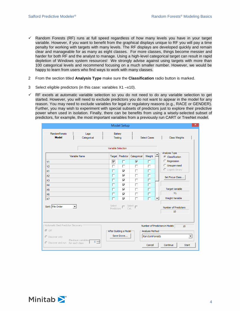
✓ Random Forests (RF) runs at full speed regardless of how many levels you have in your target variable. However, if you want to benefit from the graphical displays unique to RF you will pay a time penalty for working with targets with many levels. The RF displays are developed quickly and remain clear and manageable for as many as eight classes. For more classes, things become messier and harder for both RF and the analyst to manage. Using a high-level categorical target can result in rapid depletion of Windows system resources! We strongly advise against using targets with more than 100 categorical levels and recommend focusing on a much smaller number. However, we would be happy to learn from users who find ways to work with many classes.

2 From the section titled Analysis Type make sure the Classification radio button is marked.

3 Select eligible predictors (in this case: variables X1 –x10).

✓ RF excels at automatic variable selection so you do not need to do any variable selection to get started. However, you will need to exclude predictors you do not want to appear in the model for any reason. You may need to exclude variables for legal or regulatory reasons (e.g., RACE or GENDER). Further, you may wish to experiment with special subsets of predictors just to explore their predictive power when used in isolation. Finally, there can be benefits from using a wisely-selected subset of predictors, for example, the most important variables from a previously run CART or TreeNet model.


5

Model Setup – Class Weights

Class weights are used to compensate for highly unequal class sample sizes. The default is always

BALANCED. The available alternatives are listed on the Class Weights tab:

BALANCED: Target classes are automatically reweighted to achieve equal size (balance).

UNIT: Target classes are un-weighted. Larger target classes have proportionally greater influence

on the model.

SPECIFY: Specify class weights for each target level. Class weights are set to a value selected by

the analyst.

We recommend the BALANCED default. When the target class sample sizes are unequal, Random Forests will still give equal attention to the rare class (or classes).

Class weights can have a considerable impact on RF results and are worth experimenting with. The greater the class weight the harder RF will work to classify that class correctly. Suppose you have a binary target with 90% NO and 10% YES values. The default Class Weights generated by BALANCED will be 1 for NO and 9 for YES. You might try SPECIFY to reset the YES Class Weight to values such as 6 or even 15 or 20. There is no way to calculate the optimal Class Weights in advance of an RF run, so you will want to run some experiments.

CW BALANCED


6

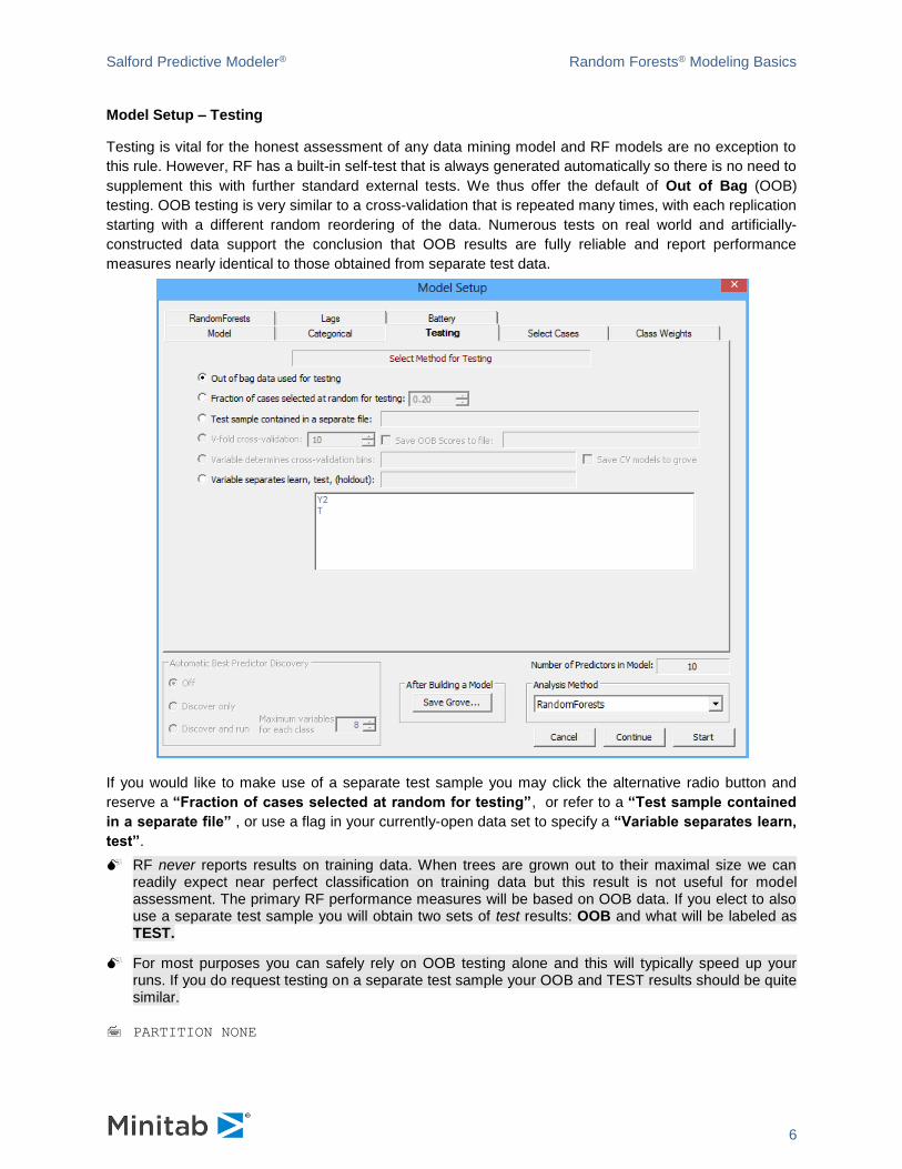
Model Setup – Testing

Testing is vital for the honest assessment of any data mining model and RF models are no exception to

this rule. However, RF has a built-in self-test that is always generated automatically so there is no need to

supplement this with further standard external tests. We thus offer the default of Out of Bag (OOB)

testing. OOB testing is very similar to a cross-validation that is repeated many times, with each replication

starting with a different random reordering of the data. Numerous tests on real world and artificially-

constructed data support the conclusion that OOB results are fully reliable and report performance

measures nearly identical to those obtained from separate test data.

If you would like to make use of a separate test sample you may click the alternative radio button and

reserve a “Fraction of cases selected at random for testing”, or refer to a “Test sample contained

in a separate file” , or use a flag in your currently-open data set to specify a “Variable separates learn,

test”.

RF never reports results on training data. When trees are grown out to their maximal size we can readily expect near perfect classification on training data but this result is not useful for model assessment. The primary RF performance measures will be based on OOB data. If you elect to also use a separate test sample you will obtain two sets of test results: OOB and what will be labeled as TEST.

For most purposes you can safely rely on OOB testing alone and this will typically speed up your runs. If you do request testing on a separate test sample your OOB and TEST results should be quite similar.

PARTITION NONE


7

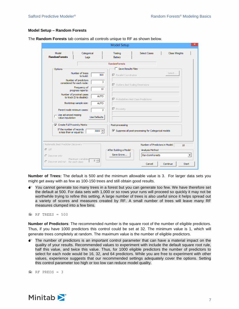
Model Setup – Random Forests

The Random Forests tab contains all controls unique to RF as shown below.

Number of Trees: The default is 500 and the minimum allowable value is 3. For larger data sets you

might get away with as few as 100-150 trees and still obtain good results.

You cannot generate too many trees in a forest but you can generate too few. We have therefore set the default at 500. For data sets with 1,000 or so rows your runs will proceed so quickly it may not be worthwhile trying to refine this setting. A large number of trees is also useful since it helps spread out a variety of scores and measures created by RF. A small number of trees will leave many RF measures clumped into a few bins.

RF TREES = 500

Number of Predictors: The recommended number is the square root of the number of eligible predictors.

Thus, if you have 1000 predictors this control could be set at 32. The minimum value is 1, which will

generate trees completely at random. The maximum value is the number of eligible predictors.

The number of predictors is an important control parameter that can have a material impact on the quality of your results. Recommended values to experiment with include the default square root rule, half this value, and twice this value. Thus, for 1000 eligible predictors the number of predictors to select for each node would be 16, 32, and 64 predictors. While you are free to experiment with other values, experience suggests that our recommended settings adequately cover the options. Setting this control parameter too high or too low can reduce model quality.

RF PREDS = 3


8

Frequency of Reports: This option is primarily for batch processing of large data sets. If set to 1, RF

summarizes its progress after every tree in the classic text output. This is useful for monitoring runs that

may require several hours to complete.

RF LOOK = 10

Number of Proximal Cases to Track: This control has no bearing whatever on model construction or on

accuracy. Instead, it influences some of the reports and displays relating to clustering and outlier

identification. If the number is set to zero, many of the graphical displays are disabled but predictive

results can be completed much more quickly. After a model is complete, if this control is not zero, RF

computes how often any pair of training data records ends up in the same terminal in an RF tree. The

Number of Proximal Cases control determines how many of the closest “neighbors” are kept track of. If

this number is set to a low value, detailed proximity information is maintained for only a few nearest

neighbors for each record. If it is set to a larger number, exact proximities are available for many more

record pairs.

The automatic setting tracks all neighbors for small data sets and gradually scales back as the number of

training records grows. Remember, if you have 30,000 training records and track the closest 1,000

neighbors for every record you are looking at 30 million items of information. Managing this much detail

requires considerable resources of both computation time and memory.

If the automatic setting results in a failure to produce the MDS scaling results you might wish to select an explicitly modest number such as the 200 we display in the example.

RF PROXIMAL = AUTO

Bootstrap sample Size: Our bootstrap sample is a sampling from the training data with replacement.

This allows some training data records to be selected more than once and results in a reweighting of the

data as well as random sampling of the data for each RF tree. Normally, the bootstrap is the same size as

the original training data. If you start with 1,000 training data records then by default each bootstrap

sample will contain 1,000 records. For smaller data sets we certainly recommend using the default.

You might be tempted to set this control parameter to a smaller number if you are working with a large

training file. For example, you might decide to set this parameter to 30,000 when working with a 200,000

record file.

Reducing the Bootstrap Sample Size may not be a good idea and may not save you any compute time. Predictive accuracy can decline with the smaller sample and you may need to grow more trees to get adequate coverage for every record in the original training data set. If you think your file is too large for direct analysis you should instead consider trimming it first and then allowing each tree to be grown on a the full scaled-back sample size.

RF BOOTSTRAP = 30000

Parent node minimum cases: The default is 2 and we advise against changing this value. RF gives best

results if trees are grown out to the largest size possible. If you are concerned that the RF trees are

unmanageably large and you insist on growing smaller trees you are probably better off working with a

smaller training file and getting automatically smaller trees as a result, leaving the Parent node minimum

at its default value.


9

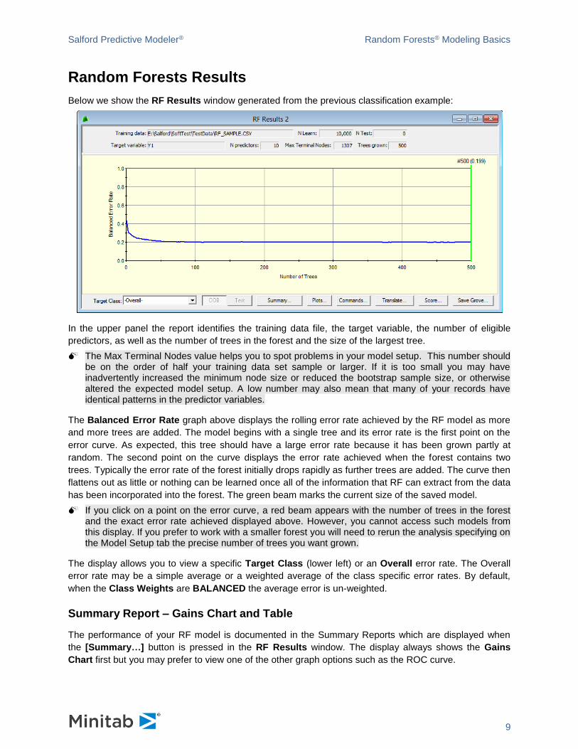
Random Forests Results

Below we show the RF Results window generated from the previous classification example:

In the upper panel the report identifies the training data file, the target variable, the number of eligible

predictors, as well as the number of trees in the forest and the size of the largest tree.

The Max Terminal Nodes value helps you to spot problems in your model setup. This number should be on the order of half your training data set sample or larger. If it is too small you may have inadvertently increased the minimum node size or reduced the bootstrap sample size, or otherwise altered the expected model setup. A low number may also mean that many of your records have identical patterns in the predictor variables.

The Balanced Error Rate graph above displays the rolling error rate achieved by the RF model as more

and more trees are added. The model begins with a single tree and its error rate is the first point on the

error curve. As expected, this tree should have a large error rate because it has been grown partly at

random. The second point on the curve displays the error rate achieved when the forest contains two

trees. Typically the error rate of the forest initially drops rapidly as further trees are added. The curve then

flattens out as little or nothing can be learned once all of the information that RF can extract from the data

has been incorporated into the forest. The green beam marks the current size of the saved model.

If you click on a point on the error curve, a red beam appears with the number of trees in the forest and the exact error rate achieved displayed above. However, you cannot access such models from this display. If you prefer to work with a smaller forest you will need to rerun the analysis specifying on the Model Setup tab the precise number of trees you want grown.

The display allows you to view a specific Target Class (lower left) or an Overall error rate. The Overall

error rate may be a simple average or a weighted average of the class specific error rates. By default,

when the Class Weights are BALANCED the average error is un-weighted.

Summary Report – Gains Chart and Table

The performance of your RF model is documented in the Summary Reports which are displayed when

the [Summary…] button is pressed in the RF Results window. The display always shows the Gains

Chart first but you may prefer to view one of the other graph options such as the ROC curve.


10

The graph displays:

When the [Gains] button is pressed – Cum % Target versus Cum % Pop.

When the [Lift] button is pressed – Lift Pop versus Cum % Pop.

When the [Cum. Lift] button is pressed – Cum Lift versus Cum % Pop.

The number of bins can be changed using the control.

When the test data are available, both OOB and TEST gains charts can be displayed using either the

[OOB] or the [Test] buttons.

Summary Report – Variable Importance

RF includes two methods for measuring the importance of a variable or how much it contributes to

predictive accuracy. The default method, the Gini, is similar in spirit to the original CART method. For

every node split by a variable in every tree in the forest we have a measure of how much the split

improved the separation of the classes. Cumulating these improvements leads to scores that are then

standardized. The most important variable always gets a score of 100.00 regardless of the overall quality

of the model.


11

An alternative measure of importance based on empirical testing is called the Standard method. For

each tree in the forest we test a variable by first scrambling its values and then measuring how much this

causes model accuracy to decline. The logic is fairly compelling: if we can substitute incorrect values for a

variable and still find that we can predict the target accurately, then that variable cannot have much

relevance to predicting the outcome. But if such data alteration causes a sharp deterioration in our ability

to predict accurately then the variable is clearly valuable. This method is used to rank every variable and

calibrate a score. As usual, all importance scores are rescaled to have values between 0 and 100.

Summary Report – Prediction Success

The final Summary Report displays the Prediction Success tab (also known as the confusion matrix) for

both OOB and TEST samples. The Prediction Success table shows whether Random Forests is tending

to concentrate its misclassifications in specific classes and, if so, where the misclassifications are

occurring.

A prediction success table is displayed below:


12

ACTUAL CLASS Class level

TOTAL CASES Total number of cases in the class

PERCENT CORRECT Percent of cases for the class that were classified correctly

Number of Class -1 cases classified in each class (-1, +1)

Number of Class +1 cases classified in each class (-1, +1)

To switch to the TEST sample prediction success table, click on [TEST] and, similarly, to view row or

column percentages rather than counts, click [Row %] or [Column %]

Plots

The various plots produced by RF are discussed in the several detailed examples included in Chapter 7

of the Random Forests Manual: An Implementation of Leo Breiman’s RF.

Saving a Model

Any model can be saved for further examination at a later time or to be used for prediction. At the bottom

left of the RandomForests Results you will see a Save Grove button. Click on this and provide a name

and location for the grove file. Your model can then be retrieved to display all the results discussed so

far.


13

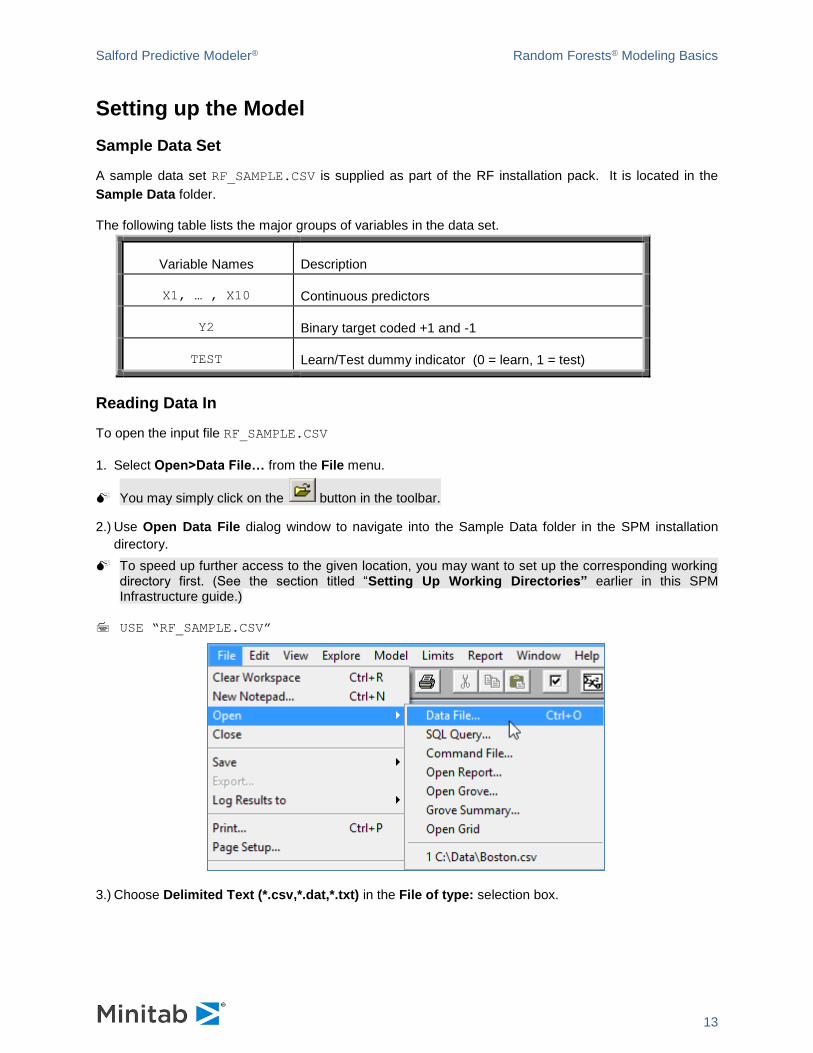
Setting up the Model

Sample Data Set

A sample data set RF_SAMPLE.CSV is supplied as part of the RF installation pack. It is located in the

Sample Data folder.

The following table lists the major groups of variables in the data set.

Variable Names Description

X1, … , X10 Continuous predictors

Y2 Binary target coded +1 and -1

TEST Learn/Test dummy indicator (0 = learn, 1 = test)

Reading Data In

To open the input file RF_SAMPLE.CSV

1. Select Open>Data File… from the File menu.

You may simply click on the button in the toolbar.

2.) Use Open Data File dialog window to navigate into the Sample Data folder in the SPM installation

directory.

To speed up further access to the given location, you may want to set up the corresponding working directory first. (See the section titled “Setting Up Working Directories” earlier in this SPM Infrastructure guide.)

USE “RF_SAMPLE.CSV”

3.) Choose Delimited Text (*.csv,*.dat,*.txt) in the File of type: selection box.


14

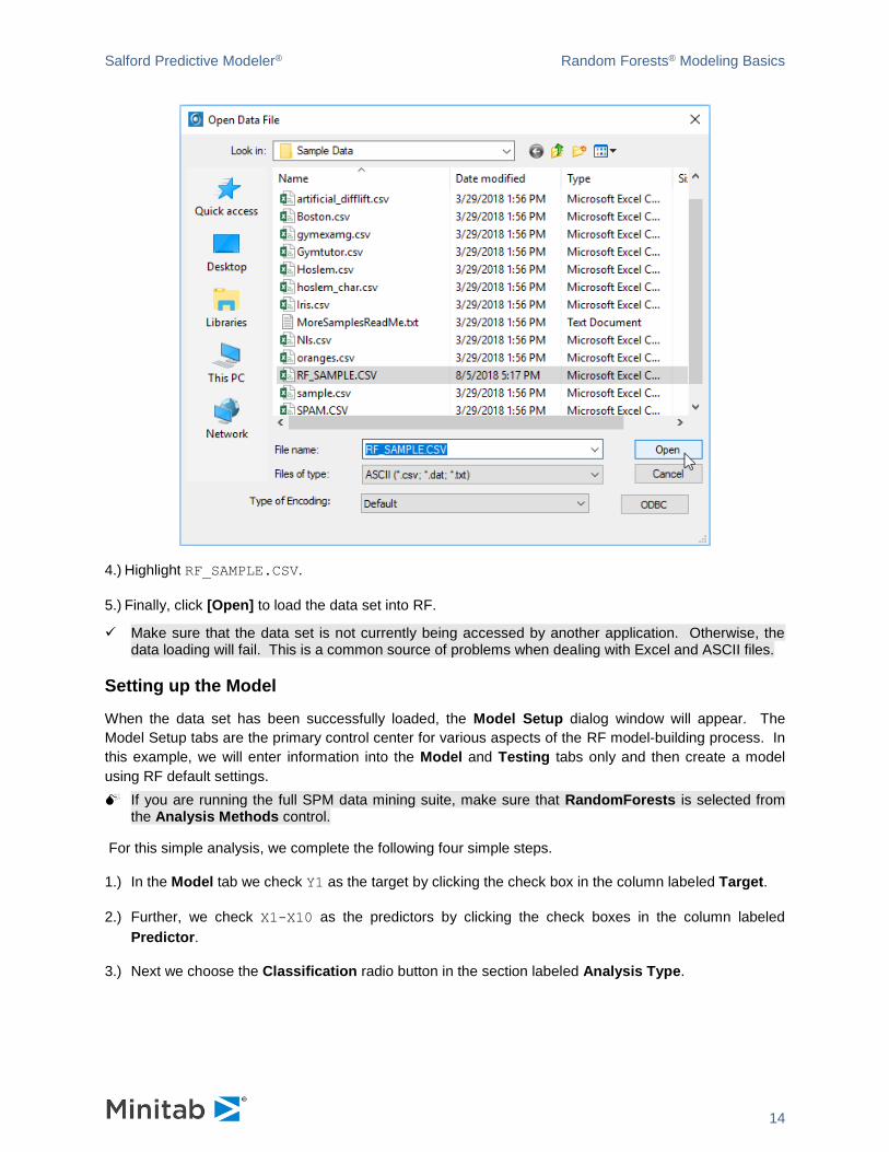
4.) Highlight RF_SAMPLE.CSV.

5.) Finally, click [Open] to load the data set into RF.

✓ Make sure that the data set is not currently being accessed by another application. Otherwise, the data loading will fail. This is a common source of problems when dealing with Excel and ASCII files.

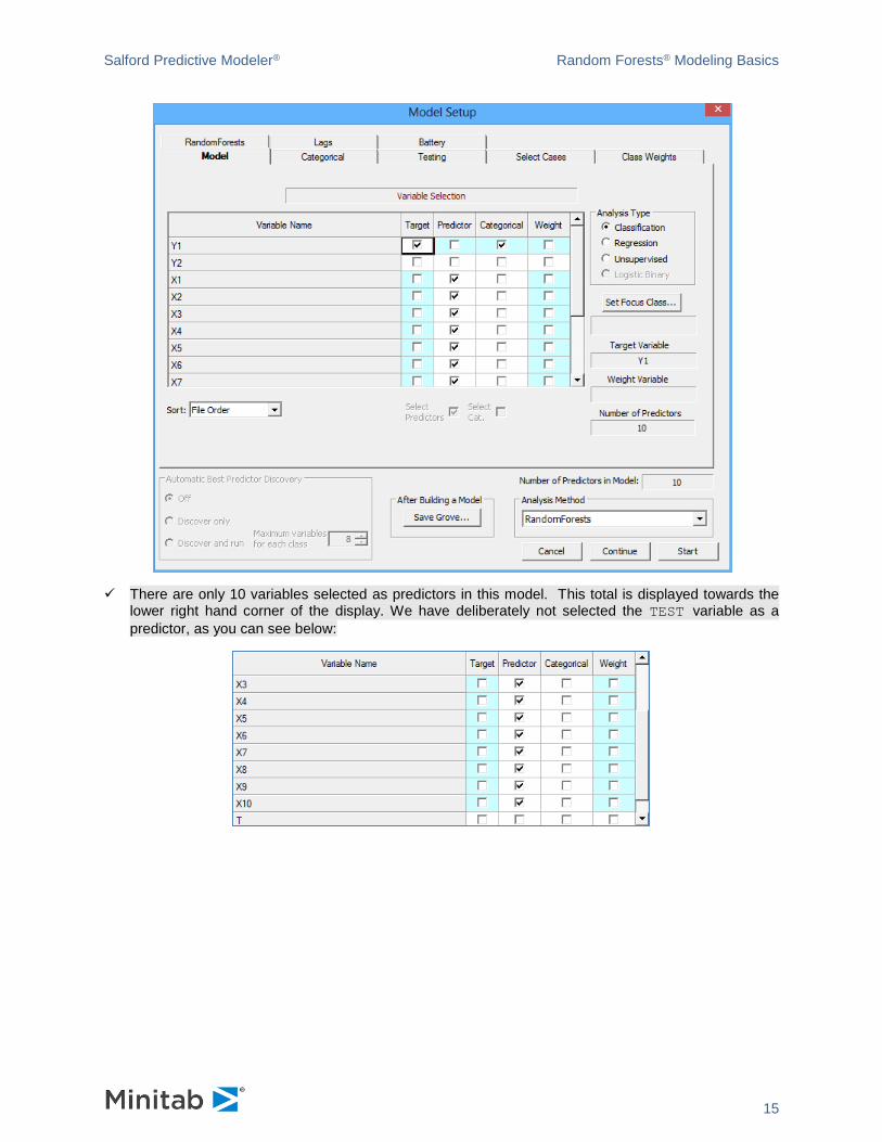
Setting up the Model

When the data set has been successfully loaded, the Model Setup dialog window will appear. The

Model Setup tabs are the primary control center for various aspects of the RF model-building process. In

this example, we will enter information into the Model and Testing tabs only and then create a model

using RF default settings.

If you are running the full SPM data mining suite, make sure that RandomForests is selected from the Analysis Methods control.

For this simple analysis, we complete the following four simple steps.

1.) In the Model tab we check Y1 as the target by clicking the check box in the column labeled Target.

2.) Further, we check X1-X10 as the predictors by clicking the check boxes in the column labeled

Predictor.

3.) Next we choose the Classification radio button in the section labeled Analysis Type.


15

✓ There are only 10 variables selected as predictors in this model. This total is displayed towards the lower right hand corner of the display. We have deliberately not selected the TEST variable as a

predictor, as you can see below:


16

4.) Select the Testing tab and choose the Variable separates learn and test samples radio button.

Choose the variable TEST in the selection list box.


17

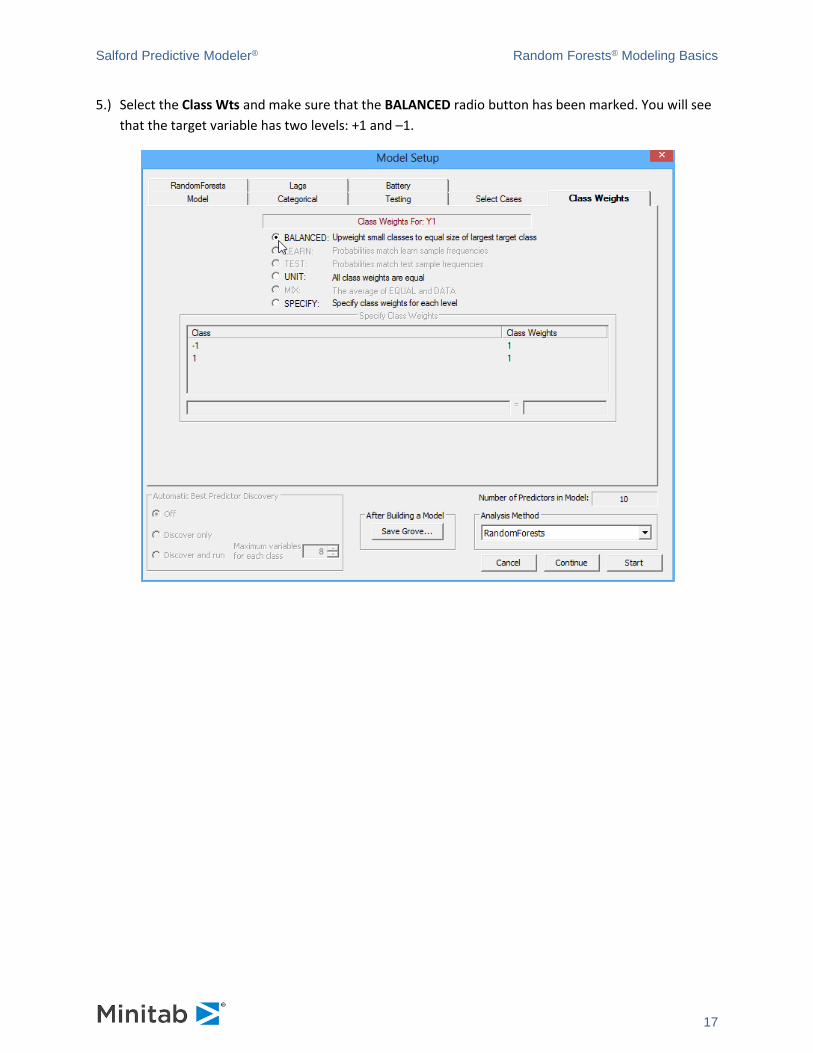
5.) Select the Class Wts and make sure that the BALANCED radio button has been marked. You will see

that the target variable has two levels: +1 and –1.


18

6.) Finally, select the RandomForests tab and set the Number of proximal cases to track to 200.

Normally you will not need to change this value but we will do so just for this example. All other RF

settings will be left at their default values.

We are now ready to start our RF run.

Running RF

To begin the RF analysis, click the [Start] button. A progress indicator will appear on the screen while

the model is being built, letting you know how many trees have been completed, how much time has

elapsed and approximately how long to completion.


19

Once the analysis is complete, text output will appear in the Output window, and a new window, RF

Results, opens.

The top portion contains key information about this analysis including the name of the training data file,

the target variable, the number of eligible predictors, the number of nodes in the largest tree grown, and

the number of trees grown. Here we grew the default 500 trees.

The bottom portion graphically displays a running relative rate for the RF model. It begins with the first

tree having an average error rate of about .45 and ends with an average error rate of .233. This statistic is

displayed above the green bar and describes the model with 500 trees. When class weights are

BALANCED, the Overall error rate is a simple average of the error rates in each class. If you select a

specific Target Class in the display above you can see that the error rates are about .280 and .185 for

the –1 and +1 classes, respectively. The error rate displayed above is based on the OOB or “Out of Bag”

self testing which is much like a repeated cross validation. Usually OOB error rates are so reliable that

we do not need a separate test sample. Nonetheless, we did use a test sample for this run and its error

curve is shown next. Observe that the RF model appears to be even more accurate on the test sample

than on the OOB data. This is not an unusual outcome.


20

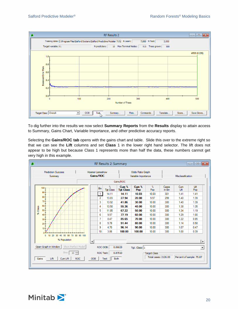
To dig further into the results we now select Summary Reports from the Results display to attain access

to Summary, Gains Chart, Variable Importance, and other predictive accuracy reports.

Selecting the Gains/ROC tab opens with the gains chart and table. Slide this over to the extreme right so

that we can see the Lift columns and set Class 1 in the lower right hand selector. The lift does not

appear to be high but because Class 1 represents more than half the data, these numbers cannot get

very high in this example.


21

Now select the Prediction Success tab where you can see that the RF model achieves a classification

accuracy of 96.28% for the –1 and 55.63% for the +1 class. Results are similar for the Test sample.

Moving on to the Variable Importance tab we obtain a ranking of the contribution of each variable to

model accuracy. We have selected the Gini measure of variable importance for convenience. The

Standard measure is an alternative approach described later in this manual.


22

We now return to the Results window so that we can select the Plots that contain further model reports.

When the Plots button is clicked you should see a graphs control like the one below:

This RF Plots Toolbox is your RF graphics control center used for selecting and modifying all of the RF

displays. First select Parallel Coordinate from the upper panel of the Toolbox to get the next display.


23

This display summarizes the predictor profile for the most probable members of each class. RF

automatically scores every record in the train and test samples with a probability. The 25 records with the

highest probabilities of being a class +1 are selected and summarized in the blue line above, while the 25

records with the highest probabilities of being a class –1 are summarized in the red line. The variables

are listed in order of importance, but you can choose other orderings from the Sort Variables control in

the lower right hand corner of the display.

We read this graph as follows: comparing the “most probable” members of each class we see that the –1

class shows a much lower value of both X1 and X2 and a slightly lower X4 and X8. Otherwise, the two

groups are fairly similar in their values on the other variables. This graph plots all variables on a [0,1]

using 0 for the minimum and 1 for the maximum seen in the overall training data. When variables show

large differences between the classes they appear to be useful discriminators in isolation. When the

variable values are close together the variables do their work in interactions with other variables. In this

example only a few variables are important so it is not surprising to see that the unimportant variables

have similar values across the two groups.

You can vary the display by selecting options from the controls at the bottom of the Parallel Coordinate

graph:


24

By default we display the median values for each class. However, you may elect to see the quartiles, min,

max, or all the records (Detail). When there are two classes the Most and Least buttons give you the

same display, but with three or more classes the least likely members of one class are not necessarily the

most likely of a single other class, so the two displays offer alternative views of the results. The prototypes

are an experimental offering that is best deferred to a later discussion.

RF is able to generate a “proximity” or similarity measure for any two records in the training data. Briefly

stated, we track which terminal node a record ends up in for every tree in the forest. Two records are

“close” to each other in RF terms if they often end up in the same terminal node. In this example we grew

500 trees, and we count the number of terminal matches achieved for every pair of records. Because the

match rate can be between 0 (no matches) and 500 (match on every tree) we have a broad range of

measures of proximity. This measure is rescaled to lie in the [0,1] interval; for some purposes it is

inverted to measure a distance or dissimilarity.

These proximities are the basis of a number of important RF outputs. First, RF can produce a complete

proximity matrix for the entire data set. When the training is modest in size, for example, 1,000 records,

the full matrix is 1,000 x 1,000 because it has to record the similarity between every pair of records.

Although this matrix contains one million elements it is readily managed and displayed on a 2.0 Ghz

Pentium IV or similar machine. However, for larger data sets this matrix quickly grows too large. For

example, a 100,000 record sample would produce a 10 trillion (10,000 million) matrix. We therefore

recommend that you request the full matrix only for training samples of 3,000 records or less. However,

we still track and make use of the proximity information for much larger samples, including samples with

well over 100,000 records. But we have to resort to some shortcuts and compression devices to manage

such huge volumes of information.

The display we look at next is one that generally would be available only for smaller data sets because it

displays the full proximity matrix. From the RF Plots Toolbox select the


25

This display uses bright coloring to signify that an element in the matrix has a large number, while dim or

dark coloring signifies a small number. Bright patches represent groups of records that are “close” to

each other and that may represent clusters.

NOTE: To enhance this display we set the Max control to 0.30 (by dragging the marker and using arrow

keys for fine tuning). By lowering Max we make it easier for a point in the display to light up. The Min

control switches low values off entirely, turning them black.

The proximity matrix displays the complete training sample. In this example the matrix is 708 rows by 708

columns, and although it is “square” the image is always wider than tall. The records are first sorted to

gather potential clusters together. Records that are close to many other records are at the upper right

hand corner of their class and records that have few close neighbors are at the lower left hand corner of

their class. There are 211 –1 (reds) and 497 +1 (blues). For other real world examples see Chapter 7 of

the Random Forests Manual: An Implementation of Leo Breiman’s RF which delves further into

extracting useful information from such displays.

✓ By default this matrix is not stored or calculated if the training sample has more than 3000 records. You can change this limit to a higher value if you are willing to wait for the extensive post-processing of the RF forest.

We next bring up the Outlier Frequency Table from the graphics Toolbox. Outliers are defined as

records that on average are far away from other members of their own class. They might have some very

close neighbors because they may be members of an outlier cluster, but on the whole they are far away

from the bulk of their own class. For every record, we calculate an average distance to all other members

of its own class, and then compute a robust standardized distance using the median and interquartile

range. Current RF doctrine holds that an outlier score of 10 on this scale indicates a genuine anomaly,


26

but there is nothing sacrosanct about this threshold. Use the outlier scores as a guide to further data

examination. For our example we obtain two displays:

This histogram reports that there are only a few records with a greater than 10 outlier score. To suppress

the tall bar for the [0,1) interval select 5 or fewer in the Show Last control at the bottom of the screen.

Next select the Outliers from the graphics Toolbox:


27

This lists the outlier score for every record in the training sample, here sorted by descending outlier value.

By hovering your mouse pointer over any bar displays, you will get results in greater detail for the record

in question.

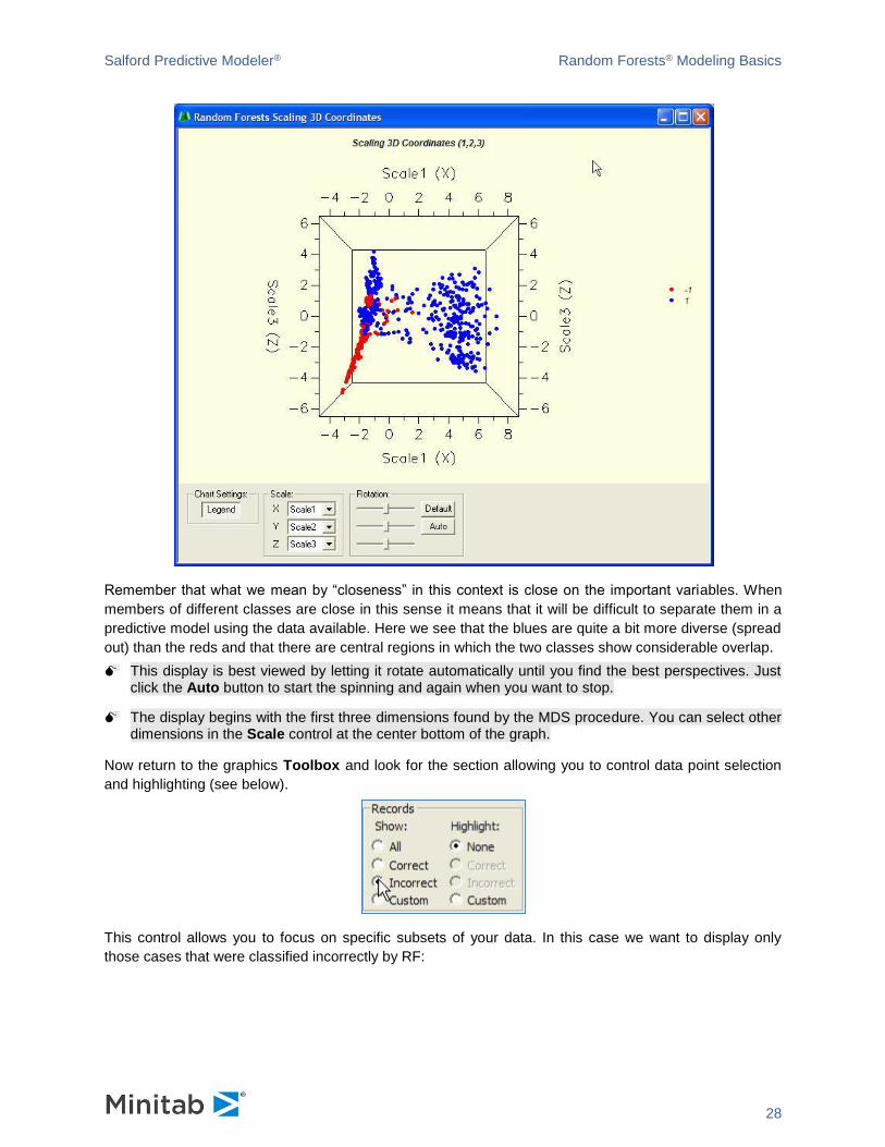
The final displays are primarily cluster related and are based on Multi-Dimensional Scaling (MDS). MDS

offers an alternative way to visualize the proximity matrix and spot potential clusters, especially when the

training sample is large. We begin with the Scaling 3D Coordinates. Simply put, the MDS display

attempts to summarize the proximity matrix by plotting points close together only if they are close together

in the proximity matrix, and otherwise plotting them far apart. In general, the display attempts to preserve

distance rankings. In the graph below we see that by and large the reds and blues occupy fairly distinct

locations, with only one region of overlap.


28

Remember that what we mean by “closeness” in this context is close on the important variables. When

members of different classes are close in this sense it means that it will be difficult to separate them in a

predictive model using the data available. Here we see that the blues are quite a bit more diverse (spread

out) than the reds and that there are central regions in which the two classes show considerable overlap.

This display is best viewed by letting it rotate automatically until you find the best perspectives. Just click the Auto button to start the spinning and again when you want to stop.

The display begins with the first three dimensions found by the MDS procedure. You can select other dimensions in the Scale control at the center bottom of the graph.

Now return to the graphics Toolbox and look for the section allowing you to control data point selection

and highlighting (see below).

This control allows you to focus on specific subsets of your data. In this case we want to display only

those cases that were classified incorrectly by RF:


29

From this we can see the dense region that RF has carved out for the reds, meaning that all blues falling

in that region are misclassified. This display should be rotated to get a more complete 3D view.

Now change the display so that we show All points but highlight the incorrect. This makes the correctly

classified points smaller.

This concludes our introductory overview of the RF software. We have not discussed every control or

every graph or report produced by RF_ but this should be enough to get you started. See Chapter 7 of

the Random Forests Manual: An Implementation of Leo Breiman’s RF which offers other

examples and elaborates on RF interpretation and getting the most out of the technology.

Documents

Random Forests® Modeling Basics - minitab.com · Salford Predictive Modeler® Random Forests® Modeling Basics 7 Model Setup – Random Forests The Random Forests tab contains all