Turk J Phys

30 (2006) , 349 – 378.

c© TUBITAK

Ramifications of Lineland

Daniel GRUMILLER1, Rene MEYER1,2

1Institute for Theoretical Physics, University of Leipzig Augustusplatz 10-11,D-04109 Leipzig-GERMANY

e-mail: grumiller@itp.uni-leipzig.de2Max Planck Institute for Mathematics in the Sciences Inselstrasse 22,

D-04103 Leipzig-GERMANYe-mail: Rene.Meyer@itp.uni-leipzig.de

Received 14.04.2006

Abstract

A non-technical overview on gravity in two dimensions is provided. Applications discussed in this work

comprise 2D type 0A/0B string theory, Black Hole evaporation/thermodynamics, toy models for quantum

gravity, for numerical General Relativity in the context of critical collapse and for solid state analogues

of Black Holes. Mathematical relations to integrable models, non-linear gauge theories, Poisson-sigma

models, KdV surfaces and non-commutative geometry are presented.

Key Words: Black Holes in String Theory, 2D Gravity, Integrable Models.

1. Introduction

The study of gravity in 2D — boring to some, fascinating to others [1] — has the undeniable disadvantageof eliminating a lot of structure that is present in higher dimensions; for instance, the Riemann tensoris determined already by the Ricci scalar, i.e., there is no Weyl curvature and no trace-free Ricci part.On the other hand, it has the undeniable advantage of eliminating a lot of structure that is present inhigher dimensions; for instance, non-perturbative results may be obtained with relative ease due to technicalsimplifications, thus allowing one to understand some important conceptual issues arising in classical andquantum gravity which are universal and hence of relevance also for higher dimensions.

The scope of this non-technical overview is broad rather than focussed, since there exist already variousexcellent reviews and textbooks presenting the technical pre-requisites in detail,1 and because the broadnessenvisaged here may lead to a cross-fertilization between otherwise only loosely connected communities. Somerecent results are presented in more detail. It goes without saying that the topics selected concur with theauthors’ preferences; by no means it should be concluded that an issue or a reference omitted here is devoidof interest.

The common link between all applications mentioned here is 2D dilaton gravity,2

S2DG =12

∫d2x√−g

[XR + U(X) (∇X)2 − 2V (X)

], (1)

1For instance, the status of the field in the late 1980ies is summarized in [2].2The 2D Einstein-Hilbert action will not be discussed except in section 6.1.

349

GRUMILLER, MEYER

the action of which depends functionally on the metric gµν and on the scalar field X. Note that veryoften, in particular in the context of string theory, the field redefinition X = e−2φ is employed; the fieldφ is the dilaton of string theory, hence the name “dilaton gravity”. However, it is emphasized that thenatural interpretation of X need not be the one of a dilaton field — it may also play the role of surfacearea, dual field strength, coordinate of a suitable target space or black hole (BH) entropy, depending onthe application. The curvature scalar R and covariant derivative ∇ are associated with the Levi-Civitaconnection and Minkowskian signature is implied unless stated otherwise. The potentials U , V define themodel; several examples will be provided below. A summary is contained in table 1.

This proceedings contribution is organized as follows: section 2 is devoted to a reformulation of (1) asa non-linear gauge theory, which considerably simplifies the construction of all classical solutions; section3 discusses applications in 2D string theory; section 4 summarizes applications in BH physics; section 5demonstrates how to reconstruct geometry from matter in a quantum approach; section 6 contains not onlymathematical issues but also some open problems.

2. Gravity as non-linear gauge theory

It has been known for a long time how to obtain all classical solutions of (1) not only locally, but globally.Two ingredients turned out to be extremely useful: a reformulation of (1) as a first order action and theimposition of a convenient (axial or Eddington-Finkelstein type) gauge, rather than using conformal gauge.3

Subsequently we will briefly recall these methods. For a more comprehensive review cf. [4].

Table 1. Selected list of models

Model (cf. (1) or (3)) U(X) V (X) w(X) (cf. (4))

1. Schwarzschild [5] − 12X −λ2 −2λ2

√X

2. Jackiw-Teitelboim [6, 7] 0 −ΛX −12ΛX2

3. Witten BH/CGHS [8, 9] − 1X

−2b2X −2b2X4. CT Witten BH [8, 9] 0 −2b2 −2b2X5. SRG (D > 3) − D−3

(D−2)X −λ2X(D−4)/(D−2) −λ2D−2D−3X

(D−3)/(D−2)

6. (A)dS2 ground state [10] − aX −B

2 X a = 2 : − B2(2−a)X

2−a

7. Rindler ground state [11] − aX −B

2 Xa −B

2 X

8. BH attractor [12] 0 −B2X

−1 −B2 lnX

9. All above: ab-family [13] − aX −B

2 Xa+b b = −1 : − B

2(b+1)Xb+1

10. Liouville gravity [14] a beαX a = −α : ba+αe

(a+α)X

11. Scattering trivial [15] generic 0 const.12. Reissner-Nordstrom [16] − 1

2X −λ2 + Q2

X −2λ2√X − 2Q2/

√X

13. Schwarzschild-(A)dS [17] − 12X −λ2 − X −2λ2

√X − 2

3X3/2

14. Katanaev-Volovich [18] α βX2 − Λ∫ X

eαy(βy2 − Λ) dy15. Achucarro-Ortiz [19] 0 Q2

X − J4X3 − ΛX Q2 lnX + J

8X2 − 12ΛX2

16. KK reduced CS [20, 21] 0 12X(c −X2) −1

8 (c−X2)2

17. Symmetric kink [22] generic −XΠni=1(X2 −X2

i ) cf. [22]18. 2D type 0A/0B [23, 24] − 1

X−2b2X + b2q2

8π−2b2X + b2q2

8πlnX

19. exact string BH[25, 26] (31) (31) (33)

3In string theory almost exclusively conformal gauge is used. A notable exception is [3].

350

GRUMILLER, MEYER

2.1. First order formulation

The Jackiw-Teitelboim model (cf. the second model in table (1)) allows a gauge theoretic formulationbased upon (A)dS2,

[Pa, Pb] = ΛεabJ , [Pa, J ] = εabPb , (2)

with Lorentz generator J , translation generators Pa and Λ = 0. A corresponding first order action, S =∫XAF

A, has been introduced in [27]. The field strength F = dA+[A,A]/2 contains the SO(1, 2) connectionA = eaPa+ωJ , and the Lagrange multipliersXA transform under the coadjoint representation. This exampleis exceptional insofar as it allows a formulation in terms of a linear (Yang-Mills type) gauge theory. Similarly,the fourth model in table 1 allows a gauge theoretic formulation [28] based upon the centrally extendedPoincare algebra [29]. The generalization to non-linear gauge theories [30] allowed a comprehensive treatmentof all models (1) with U = 0, which has been further generalized to U = 0 in [31]. The corresponding firstorder gravity action

SFOG = −∫ [

XaTa +XR + ε

(X+X−U(X) + V (X)

)](3)

is equivalent to (1) (with the same potentials U, V ) upon elimination of the auxiliary fields Xa and thetorsion-dependent part of the spin-connection. Here is our notation: ea = eaµdx

µ is the dyad 1-form. Latinindices refer to an anholonomic frame, Greek indices to a holonomic one. The 1-form ω represents thespin-connection ωa

b = εabω = εabωµ dxµ with the totally antisymmetric Levi-Civita symbol εab (ε01 = +1).With the flat metric ηab in light-cone coordinates (η+− = 1 = η−+, η++ = 0 = η−−) it reads ε±± = ±1.The torsion 2-form present in the first term of (3) is given by T± = (d±ω) ∧ e±. The curvature 2-form Ra

b

can be represented by the 2-form R defined by Rab = εabR with R = dω. It appears in the second term in

(3). Since no confusion between 0-forms and 2-forms should arise the Ricci scalar is also denoted by R. Thevolume 2-form is denoted by ε = e+ ∧ e−. Signs and factors of the Hodge-∗ operation are defined by ∗ε = 1.It should be noted that (3) is a specific Poisson-sigma model [31] with a 3D target space, with target spacecoordinates X,X±, see section 6.3 below. A second order action similar to (1) has been introduced in [32].

2.2. Generic classical solutions

It is useful to introduce the following combinations of the potentials U and V :

I(X) := exp∫ X

U(y) dy , w(X) :=∫ X

I(y)V (y) dy (4)

The integration constants may be absorbed, respectively, by rescalings and shifts of the “mass”, see equation(10) below. Under dilaton dependent conformal transformations Xa → Xa/Ω, ea → eaΩ, ω → ω +Xae

a d ln Ω/ dX the action (3) is mapped to a new one of the same type with transformed potentials U , V .Hence, it is not invariant. It turns out that only the combination w(X) as defined in (4) remains invariant,so conformally invariant quantities may depend on w only. Note that I is positive apart from eventualboundaries (typically, I may vanish in the asymptotic region and/or at singularities). One may transformto a conformal frame with I = 1, solve all equations of motion and then perform the inverse transformation.Thus, it is sufficient to solve the classical equations of motion for U = 0,

dX + X−e+ − X+e− = 0 , (5)

(d±ω)X± ∓ e±V (X) = 0 , (6)

(d±ω) ∧ e± = 0 , (7)

which is what we are going to do now. Note that the equation containing dω is redundant, whence it is notdisplayed.

351

GRUMILLER, MEYER

Let us start with an assumption: X+ = 0 for a given patch. To get some physical intuition as to what thiscondition could mean: the quantities Xa, which are the Lagrange multipliers for torsion, can be expressed asdirectional derivatives of the dilaton field by virtue of (5) (e.g. in the second order formulation a term of theform XaXa corresponds to (∇X)2). For those who are familiar with the Newman-Penrose formalism: forspherically reduced gravity the quantities Xa correspond to the expansion spin coefficients ρ and ρ′ (bothare real). If X+ vanishes a (Killing) horizon is encountered and one can repeat the calculation below withindices + and − swapped everywhere. If both vanish in an open region by virtue of (5) a constant dilatonvacuum emerges, which will be addressed separately below. If both vanish on isolated points the Killinghorizon bifurcates there and a more elaborate discussion is needed [33]. The patch implied by X+ = 0is a “basic Eddington-Finkelstein patch”, i.e., a patch with a conformal diagram which, roughly speaking,extends over half of the bifurcate Killing horizon and exhibits a coordinate singularity on the other half. Insuch a patch one may redefine e+ = X+Z with a new 1-form Z. Then (5) implies e− = dX/X+ + X−Zand the volume form reads ε = e+ ∧ e− = Z ∧ dX. The + component of (6) yields for the connectionω = −dX+/X+ +ZV (X). One of the torsion conditions (7) then leads to dZ = 0, i.e., Z is closed. Locally(in fact, in the whole patch) it is also exact: Z = du. It is emphasized that, besides the integration of (9)below, this is the only integration needed! After these elementary steps one obtains already the conformallytransformed line element in Eddington-Finkelstein (EF) gauge

ds2 = 2e+e− = 2 du dX + 2X+X− du2 , (8)

which nicely demonstrates the power of the first order formalism. In the final step the combination X+X−

has to be expressed as a function of X. This is possible by noting that the linear combination X+×[(6) with− index] + X−×[(6) with + index] together with (5) establishes a conservation equation,

d(X+X−) + V (X) dX = d(X+X− +w(X)) = 0 . (9)

Thus, there is always a conserved quantity (dM = 0), which in the original conformal frame reads

M = −X+X−I(X) − w(X) , (10)

where the definitions (4) have been inserted. It should be noted that the two free integration constantsinherent to the definitions (4) may be absorbed by rescalings and shifts of M , respectively. The classicalsolutions are labelled by M , which may be interpreted as mass (see section 4.2). Finally, one has to transformback to the original conformal frame (with conformal factor Ω = I(X)). The line element (8) by virtue of(10) may be written as

ds2 = 2I(X) du dX − 2I(X)(w(X) + M) du2 . (11)

Evidently there is always a Killing vector K · ∂ = ∂/∂u with associated Killing norm K2 = −2I(w + M).Since I = 0 Killing horizons are encountered at X = Xh where Xh is a solution of

w(Xh) +M = 0 . (12)

It is recalled that (11) is valid in a basic EF patch, e.g., an outgoing one. By redoing the derivation above,but starting from the assumption X− = 0 one may obtain an ingoing EF patch, and by gluing togetherthese patches appropriately one may construct the Carter-Penrose diagram, cf. [34, 33, 4].

As pointed out in the introduction the full geometric information resides in the Ricci scalar. The onerelated to the generic solution (11) reads

R =2

I(X)d

dX

(U(X)(M +w(X)) + I(X)V (X)

). (13)

352

GRUMILLER, MEYER

There are two important special cases: for U = 0 the Ricci scalar simplifies to R = 2V ′(X), while forw(X) ∝ 1/I(X) it scales proportional to the mass, R = 2MU ′(X)/I(X). The latter case comprises so-called Minkowskian ground state models (for examples cf. the first, third, fifth and last line in table 1). Notethat for many models in table 1 the potential U(X) has a singularity at X = 0 and consequently a curvaturesingularity arises.

2.3. Constant dilaton vacua

For sake of completeness it should be mentioned that in addition to the family of generic solutions(11), labelled by the mass M , isolated solutions may exist, so-called constant dilaton vacua (cf. e.g. [22]),which have to obey4 X = XCDV = const. with V (XCDV ) = 0. The corresponding geometry has constantcurvature, i.e., only Minkowski, Rindler or (A)dS2 are possible space-times for constant dilaton vacua.5 TheRicci scalar is determined by

RCDV = 2V ′(XCDV) = const. (14)

Examples are provided by the last eighth entries in table 1. For instance, 2D type 0A strings with an equalnumber q of electric and magnetic D0 branes (cf. the penultimate entry in table 1) allow for an AdS2 vacuumwith XCDV = q2/(16π) and RCDV = −4b2 [37].

2.4. Topological generalizations

In 2D there are neither gravitons nor photons, i.e. no propagating physical modes exist [38]. This featuremakes the inclusion of Yang-Mills fields in 2D dilaton gravity or an extension to supergravity straightforward.Indeed, both generalizations can be treated again in the first order formulation as a Poisson-sigma model,cf. e.g. [39]. In addition to M (see (10)) more locally conserved quantities (Casimir functions) may emergeand the integrability concept is extended.

As a simple example we include an abelian Maxwell field, i.e., instead of (3) we take

SMDG = −∫ [

XaTa + XR +BF + ε

(X+X−U(X,B) + V (X,B)

)], (15)

where B is an additional scalar field and F = dA is the field strength 2-form. Variation with respect toA immediately establishes a constant of motion, B = Q, where Q is some real constant, the U(1) charge.Variation with respect to B may produce a relation that allows to express B as a function of the dilaton andthe dual field strength ∗F . For example, suppose that V (X,B) = V (X)+ 1

2B2. Then, variation with respect

to B gives B = −∗F . Inserting this back into the action yields a standard Maxwell term. The solution ofthe remaining equations of motion reduces to the case without Maxwell field. One just has to replace B byits on-shell value Q in the potentials U , V .

Concerning supergravity we just mention a couple of references for further orientation [40, 41, 36].

2.5. Non-topological generalizations

To get a non-topological theory one can add scalar or fermionic matter. The action for a real, self-interacting and non-minimally coupled scalar field T ,

ST =12

∫ [F (X) dT ∧ ∗ dT + εf(X, T )

], (16)

4Incidentally, for the generic case (11) the value of the dilaton on an extremal Killing horizon is also subject to these two

constraints.5In quintessence cosmology in 4D such solutions serve as late time dS4 attractor [35]. In 2D dilaton supergravity solutions

preserving both supersymmetries are necessarily constant dilaton vacua [36].

353

GRUMILLER, MEYER

in our convention requires F < 0 for the kinetic term to have the correct sign; e.g. F = −κ or F = −κX.While scalar matter couples to the metric and the dilaton, fermions6 couple directly to the Zweibein

(A←→d B = AdB − (dA)B),

Sχ =∫ [ i

2F (X) (∗ea) ∧ (χγa

←→d χ) + εH(X)g(χχ)], (17)

but not — and this is a peculiar feature of 2D — to the spin connection. The self-interaction is at mostquartic (a constant term may be absorbed in V (X)),

g(χχ) = mχχ + λ(χχ)2 . (18)

The quartic term (henceforth: Thirring term [43]) can also be recast into a classically equivalent form byintroducing an auxiliary vector potential,

λ

∫ε(χχ)2 =

λ

2

∫[A ∧ ∗A+ 2A ∧ (∗ea)χγaχ] , (19)

which lacks a kinetic term and thus does not propagate by itself.We speak of minimal coupling if the coupling functions F (X), f(X, T ), H(X) do not depend on the

dilaton X, and of nonminimal coupling otherwise.As an illustration we present the spherically reduced Einstein-massless-Klein-Gordon model (EMKG). It

emerges from dimensional reduction of 4D Einstein-Hilbert (EH) gravity (cf. the first model in table 1) witha minimally coupled scalar field, with the choices f(X, τ ) = 0 and

w(X) = −2λ2√X , F (X) = −κX , I(X) =

1√X, (20)

where λ is an irrelevant scale parameter and κ encodes the (also irrelevant) Newton coupling. Minimallycoupled Dirac fermions in four dimensions yield upon dimensional reduction two 2-spinors coupled to eachother through intertwinor terms, which is not covered by (17) (see [44] for details on spherical reduction offields of arbitrary spin and the spherical reduced standard model).

With matter the equation of motion (6) and the conservation law (9) obtain contributions W± = δ(ST +Sχ)/δe∓ and X−W+ + X+W−, respectively, destroying integrability because Z is not closed anymore:dZ = W+ ∧ Z/X+. In special cases exact solutions can be obtained:

1. For (anti-)chiral fermions and (anti-)selfdual scalars with W+ = 0 (W− = 0) the geometric solution(8) is still valid [4] and the second equation of motion (6) implies W− = W−

u du. Such solutions havebeen studied e.g. in [45, 46]. They arise also in the Aichelburg-Sexl limit [47] of boosted BHs [48].

2. A one parameter family of static solutions of the EMKG has been discovered in [49]. Studies of staticsolutions in generic dilaton gravity may be found in [50, 51]. A static solution for the line-elementwith time-dependent scalar field (linear in time) has been discussed for the first time in [52]. It hasbeen studied recently in more detail in [53].

3. A (continuously) self-similar solution of the EMKG has been discoverd in [54].

4. Specific models allow for exact solutions even in the presence of more general matter sources; forinstance, the conformally transformed CGHS model (fourth in table 1), Rindler ground state models(seventh in table 1) and scattering trivial models (eleventh in table 1).

6We use the same definition for the Dirac matrices as in [42].

354

GRUMILLER, MEYER

3. Strings in 2D

Strings propagating in a 2D target space are comparatively simple to describe because the only propa-gating degree of freedom is the tachyon (and if the latter is switched off the theory becomes topological).Hence several powerful methods exist to describe the theory efficiently, e.g. as matrix models. In particu-lar, strings in non-trivial backgrounds may be studied in great detail. Here are some references for furtherorientation: For the matrix model description of 2D type 0A/0B string theory cf. [55, 23] (for an extensivereview on Liouville theory and its relation to matrix models and strings in 2D cf. [14]; some earlier reviewsare refs. [56]; the matrix model for the 2D Euclidean string BH has been constructed in [57]; a study ofLiouville theory from the 2D dilaton gravity point of view may be found in [58]). The low energy effectiveaction for 2D type 0A/0B string theory in the presence of RR fluxes has been studied from various aspectse.g. in [59, 23, 37, 24].

3.1. Target space formulation of 2D type 0A/0B string theory

For sake of definiteness focus will be on 2D type 0A with an equal number q of electric and magnetic D0branes, but other cases may be studied as well. For vanishing tachyon the corresponding target space actionis given by (setting κ2 = 1)

S0A =12

∫d2x√−g

[e−2φ

(R − 4 (∇φ)2 + 4b2

)− b2q2

4π

], (21)

Obviously, this is a special case of the generic model (1), with U, V given by the penultimate model intable 1, to which all subsequent considerations — in particular thermodynamical issues — apply. Note thatthe dilaton fields X and φ are related by X = exp (−2φ). The constant b2 = 2/α′ defines the physical scale.In the absence of D0 branes, q = 0, the model simplifies to the Witten BH, cf. the third line in table 1.

The action defining the tachyon sector up to second order in T is given by (cf. (16))

ST =12

∫d2x√−g [F (X)gµν (∂µT )(∂νT ) + f(X, T )] , (22)

with

F (X) = X , f(T , X) = b2T 2(X − q2

2π

). (23)

The total action is S0A + ST .

3.2. Exact string Black Hole

The exact string black hole (ESBH) was discovered by Dijkgraaf, Verlinde and Verlinde more than adecade ago [25]. The construction of a target space action for it which does not display non-localities orhigher order derivatives had been an open problem which could be solved only recently [26]. There areseveral advantages of having such an action available: the main point of the ESBH is its non-perturbativeaspect, i.e., it is believed to be valid to all orders in the string-coupling α′. Thus, a corresponding actioncaptures non-perturbative features of string theory and allows, among other things, a thorough discussion ofADM mass, Hawking temperature and Bekenstein–Hawking entropy of the ESBH which otherwise requiressome ad-hoc assumption. Therefore, we will devote some space to its description. At the perturbativelevel actions approximating the ESBH are known: to lowest order in α′ one has (21) with q = 0. Pushingperturbative considerations further Tseytlin was able to show that up to 3 loops the ESBH is consistent withsigma model conformal invariance [60]. In the strong coupling regime the ESBH asymptotes to the Jackiw–Teitelboim model [6]. The exact conformal field theory methods used in [25], based upon the SL(2,R)/U(1)

355

GRUMILLER, MEYER

gauged Wess–Zumino–Witten model, imply the dependence of the ESBH solutions on the level k. A different(somewhat more direct) derivation leading to the same results for dilaton and metric was presented in [61].For a comprehensive history and more references [62] may be consulted.

In the notation of [63] for Euclidean signature the line element of the ESBH is given by

ds2 = f2(x) dτ2 + dx2 , (24)

with

f(x) =tanh(bx)√

1− p tanh2(bx). (25)

Physical scales are adjusted by the parameter b ∈ R+ which has dimension of inverse length. The corre-

sponding expression for the dilaton,

φ = φ0 − ln cosh(bx)− 14

ln(1− p tanh2(bx)

), (26)

contains an integration constant φ0. Additionally, there are the following relations between constants,string-coupling α′, level k and dimension D of string target space:

α′b2 =1

k − 2, p :=

2k

=2α′b2

1 + 2α′b2, D − 26 + 6α′b2 = 0 . (27)

For D = 2 one obtains p = 89 , but like in the original work [25] we will treat general values of p ∈ (0; 1)

and consider the limits p → 0 and p → 1 separately: for p = 0 one recovers the Witten BH geometry; forp = 1 the Jackiw–Teitelboim model is obtained. Both limits exhibit singular features: for all p ∈ (0; 1) thesolution is regular globally, asymptotically flat and exactly one Killing horizon exists. However, for p = 0a curvature singularity (screened by a horizon) appears and for p = 1 space-time fails to be asymptoticallyflat. In the present work exclusively the Minkowskian version of (24)

ds2 = f2(x) dτ2 − dx2 , (28)

will be needed. The maximally extended space-time of this geometry has been studied in [64]. Wind-ing/momentum mode duality implies the existence of a dual solution, the Exact String Naked Singularity(ESNS), which can be acquired most easily by replacing bx→ bx+ iπ/2, entailing in all formulas above thesubstitutions sinh→ i cosh, cosh→ i sinh.

After it had been realized that the nogo result of [65] may be circumvented without introducing su-perfluous physical degrees of freedom by adding an abelian BF -term, a straightforward reverse-engineeringprocedure allowed to construct uniquely a target space action of the form (1), supplemented by aforemen-tioned BF -term,

SESBH = −∫ [

XaTa + XESBHR + ε

(X+X−UESBH + VESBH

)]−∫BF , (29)

where B is a scalar field and F = dA an abelian field strength 2-form. Per constructionem SESBH reproducesas classical solutions precisely (25)–(28) not only locally but globally. A similar action has been constructedfor the ESNS. The relation (X − γ)2 = arcsinh 2γ in conjunction with the definition γ := exp (−2φ)/B maybe used to express the auxiliary dilaton field X entering the action (1) in terms of the “true” dilaton fieldφ and the auxiliary field B. The two branches of the square root function correspond to the ESBH (mainbranch) and the ESNS (second branch), respectively:

XESBH = γ + arcsinh γ , XESNS = γ − arcsinh γ . (30)

356

GRUMILLER, MEYER

1 2 3 4 5

0.25

0.5

0.75

1

1.25

1.5

1.75

2

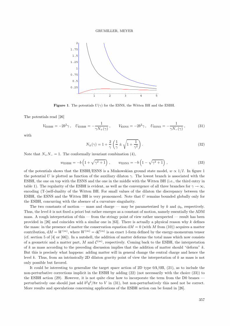
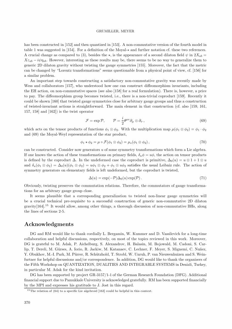
Figure 1. The potentials U(γ) for the ESNS, the Witten BH and the ESBH.

The potentials read [26]

VESBH = −2b2γ , UESBH = − 1γN+(γ)

, VESNS = −2b2γ , UESNS = − 1γN−(γ)

, (31)

with

N±(γ) = 1 +2γ

(1γ±√

1 +1γ2

). (32)

Note that N+N− = 1. The conformally invariant combination (4),

wESBH = −b(

1 +√γ2 + 1

), wESNS = −b

(1−

√γ2 + 1

), (33)

of the potentials shows that the ESBH/ESNS is a Minkowskian ground state model, w ∝ 1/I. In figure 1the potential U is plotted as function of the auxiliary dilaton γ. The lowest branch is associated with theESBH, the one on top with the ESNS and the one in the middle with the Witten BH (i.e., the third entry intable 1). The regularity of the ESBH is evident, as well as the convergence of all three branches for γ →∞,encoding (T-)self-duality of the Witten BH. For small values of the dilaton the discrepancy between theESBH, the ESNS and the Witten BH is very pronounced. Note that U remains bounded globally only forthe ESBH, concurring with the absence of a curvature singularity.

The two constants of motion — mass and charge — may be parameterized by k and φ0, respectively.Thus, the level k is not fixed a priori but rather emerges as a constant of motion, namely essentially the ADMmass. A rough interpretation of this — from the stringy point of view rather unexpected — result has beenprovided in [26] and coincides with a similar one in [63]. There is actually a physical reason why k definesthe mass: in the presence of matter the conservation equation dM = 0 (with M from (10)) acquires a mattercontribution, dM = W (m), where W (m) = dC(m) is an exact 1-form defined by the energy-momentum tensor(cf. section 5 of [4] or [66]). In a nutshell, the addition of matter deforms the total mass which now consistsof a geometric and a matter part, M and C(m), respectively. Coming back to the ESBH, the interpretationof k as mass according to the preceding discussion implies that the addition of matter should “deform” k.But this is precisely what happens: adding matter will in general change the central charge and hence thelevel k. Thus, from an intrinsically 2D dilaton gravity point of view the interpretation of k as mass is notonly possible but favored.

It could be interesting to generalize the target space action of 2D type 0A/0B, (21), as to include thenon-perturbative corrections implicit in the ESBH by adding (22) (not necessarily with the choice (23)) tothe ESBH action (29). However, it is not quite clear how to incorporate the term from the D0 branes —perturbatively one should just add b2q2/8π to V in (31), but non-perturbatively this need not be correct.More results and speculations concerning applications of the ESBH action can be found in [26].

357

GRUMILLER, MEYER

4. Black Holes

BHs are fascinating objects, both from a theoretical and an experimental point of view [67]. Many ofthe features which are generic for BHs are already exhibited by the simplest members of this species, theSchwarzschild and Reissner-Nordstrom BHs (sometimes the Schwarzschild BH even is dubbed as “Hydrogenatom of General Relativity”). Since both of them, after integrating out the angular part, belong to theclass of 2D dilaton gravity models (the first and twelfth model in table 1), the study of (3) at the classical,semi-classical and quantum level is of considerable importance for the physics of BHs.

4.1. Classical analysis

In section 2.2 it has been recalled briefly how to obtain all classical solutions in basic EF patches, (11).By looking at the geodesics of test particles and completeness properties it is straightforward to constructall Carter-Penrose diagrams for a generic model (3) (or, equivalently, (1)). For a detailed description of thisalgorithm cf. [34, 33, 4] and references therein.

4.2. Thermodynamics

Mass The question of how to define “the” mass in theories of gravity is notoriously cumbersome. Anice clarification for D = 4 is contained in [68]. The main conceptual point is that any mass definition ismeaningless without specifying 1. the ground state space-time with respect to which mass is being measuredand 2. the physical scale in which mass units are being measured. Especially the first point is emphasizedhere. In addition to being relevant on its own, a proper mass definition is a pivotal ingredient for anythermodynamical study of BHs. Obviously, any mass-to-temperature relation is meaningless without definingthe former (and the latter). For a large class of 2D dilaton gravities these issues have been resolved in[69]. One of the key ingredients is the existence [70, 71] of a conserved quantity (10) which has a deeperexplanation in the context of first order gravity [72] and Poisson-sigma models [31]. It establishes thenecessary prerequisite for all mass definitions, but by itself it does not yet constitute one. Ground stateand scale still have to be defined. Actually, one can take M from (10) provided the two ambiguities fromintegration constants in (4) are fixed appropriately. This is described in detail in appendix A of [51]. Inthose cases where this notion makes sense M then coincides with the ADM mass.

Hawking temperature There are many ways to calculate the Hawking temperature, some of theminvolving the coupling to matter fields, some of them being purely geometrical. Because of its simplicity wewill restrict ourselves to a calculation of the geometric Hawking temperature as derived from surface gravity(cf. e.g. [73]). If defined in this way it turns out to be independent of the conformal frame. However, itshould be noted that identifying Hawking temperature with surface gravity is somewhat naive for space-times which are not asymptotically flat. But the difference is just a redshift factor and for quantities likeentropy or specific heat actually (34) is the relevant quantity as it coincides with the period of Euclideantime (cf. e.g. [74]). Surface gravity can be calculated by taking the normal derivative d/ dX of the Killingnorm (cf. (11)) evaluated on one of the Killing horizons X = Xh, where Xh is a solution of (12), thus yielding

TH =1

2π

∣∣∣w′(X)∣∣∣X=Xh

. (34)

The numerical prefactor in (34) can be changed e.g. by a redefinition of the Boltzmann constant. It hasbeen chosen in accordance with refs. [75, 4].

Entropy In 2D dilaton gravity there are various ways to calculate the Bekenstein-Hawking entropy. Usingtwo different methods (simple thermodynamical considerations, i.e., dM = T dS, and Wald’s Noether charge

358

GRUMILLER, MEYER

technique [76]) Gegenberg, Kunstatter and Louis-Martinez were able to calculate the entropy for rathergeneric 2D dilaton gravity [77]: entropy equals the dilaton field evaluated at the Killing horizon,

S = 2πXh . (35)

There exist various ways to count the microstates by appealing to the Cardy formula [78] and to recoverthe result (35). However, the true nature of these microstates remains unknown in this approach, which isa challenging open problem. Many different proposals have been made [79].

Specific heat By virtue of Cs = T dS/ dT the specific heat reads

Cs = 2πw′

w′′

∣∣∣∣X=Xh

= γS TH , (36)

with γS = 4π2 sign (w′(Xh))/w′′(Xh). Because it is determined solely by the conformally invariant combi-nation of the potentials, w as defined in (4), specific heat is independent of the conformal frame, too. On acurious sidenote it is mentioned that (36) behaves like an electron gas at low temperature with Sommerfeldconstant γS (which in the present case may have any sign). If Cs is positive and CsT

2 1 one may calculatelogarithmic corrections to the canonical entropy from thermal fluctuations and finds [80]

Scan = 2πXh +32

ln∣∣∣w′(Xh)

∣∣∣− 12

ln∣∣∣w′′(Xh)

∣∣∣+ . . . . (37)

Hawking-Page like phase transition In their by now classic paper on thermodynamics of BHs in AdS,Hawking and Page found a critical temperature signalling a phase transition between a BH phase and apure AdS phase [17]. This has engendered much further research, mostly in the framework of the AdS/CFTcorrespondence (for a review cf. [81]). This transition is displayed most clearly by a change of the specificheat from positive to negative sign: for Schwarzschild-AdS (cf. the thirteenth entry in table 1) the criticalvalue of Xh is given by Xc

h = 2/3. For Xh > Xch the specific heat is positive, for Xh < Xc

h it is negative.7

By analogy, a similar phase transition may be expected for other models with corresponding behavior ofCs. Interesting speculations on a phase transition at the Hagedorn temperature Th = k/(2π) induced by atachyonic instability have been presented recently in the context of 2D type 0A strings (cf. the penultimatemodel in table 1) by Olsson [83]. From equation (22) of that work one can check easily that indeed thespecific heat (at fixed q), Cs = (q2/8)(T/Th)/(1− T/Th), changes sign at T = Th.

4.3. Semi-classical analysis

After the influential CGHS paper [9] there has been a lot of semi-classical activity in 2D, most of which issummarized in [84, 75, 4]. In many applications one considers (1) coupled to a scalar field (16) with F = const.(minimal coupling). Technically, the crucial ingredient for 1-loop effects is the Weyl anomaly (cf. e.g. [85])< Tµ

µ >= R/(24π), which — together with the semi-classical conservation equation ∇µ < Tµν >= 0 —allows to derive the flux component of the energy momentum tensor after fixing some relevant integrationconstant related to the choice of vacuum (e.g. Unruh, Hartle-Hawking or Boulware). This method goesback to Christensen and Fulling [86]. For non-minimal coupling, e.g. F ∝ X, there are some importantmodifications — for instance, the conservation equation no longer is valid but acquires a right hand sideproportional to F ′(X). The first calculation of the conformal anomaly in that case has been performed byMukhanov, Wipf and Zelnikov [87]. It has been confirmed and extended e.g. in [88].

7Actually, in the original work [17] Hawking and Page did not invoke the specific heat directly. The consideration of the

specific heat as an indicator for a phase transition is in accordance with the discussion in [82].

359

GRUMILLER, MEYER

4.4. Long time behavior

The semi-classical analysis, while leading to interesting results, has the disadvantage of becoming unreli-able as the mass of the evaporating BH drops to zero. The long time behavior of an evaporating BH presentsa challenge to theoretical physics and touches relevant conceptual issues of quantum gravity, such as theinformation paradox. There are basically two strategies: top-down, i.e., to construct first a full quantumtheory of gravity and to discuss BH evaporation as a particular application thereof, and bottom-up, i.e., tosidestep the difficulties inherent to the former approach by invoking “reasonable” ad-hoc assumptions. Thelatter route has been pursued in [12]. A crucial technical ingredient has been Izawa’s result [89] on consistentdeformations of 2D BF theory, while the most relevant physical assumption has been boundedness of theasymptotic matter flux during the whole evaporation process. Together with technical assumptions whichcan be relaxed, the dynamics of the evaporating BH has been described by means of consistent deformationsof the underlying gauge symmetries with only one important deformation parameter. In this manner anattractor solution, the endpoint of the evaporation process, has been found (cf. the eighth model in table 1).

Ideologically, this resembles the exact renormalization group approach, cf. e.g. [90, 91] and referencestherein, which is based upon Weinberg’s idea of “asymptotic safety”.8 There are, however, several conceptualand technical differences, especially regarding the truncation of “theory space”: in 4D a truncation to EHplus cosmological constant, undoubtedly a very convenient simplification, may appear to be somewhat ad-hoc, whereas in 2D a truncation to (3) comprises not only infinitely many different theories, but essentially9

all theories with the same field content as (3) and the same kind of local symmetries (Lorentz transformationsand diffeomorphisms).

The global structure of an evaporating BH can also be studied, and despite of the differences betweenvarious approaches there seems to be partial agreement on it, cf. e.g. [93, 94, 12, 95, 96, 91]. The crucialinsight might be that a BH in the mathematical sense (i.e., an event horizon) actually never forms, but onlysome trapped region, cf. figure 5 in [96].

4.5. Killing horizons kill horizon degrees

As pointed out by Carlip [97], the fact that very different approaches to explain the entropy of BHsnevertheless agree on the result urgently asks for some deeper explanation. Carlip’s suggestion was toconsider an underlying symmetry, somehow attached to the BH horizon, as the key ingredient, and he notedthat requiring the presence of a horizon imposes constraints on the physical phase space. Actually, the changeof the phase-space structure due to a constraint which imposes the existence of a horizon in space-time isan issue which is of considerable interest by itself.

In a recent work [98] we could show that the classical physical phase space is smaller as compared tothe generic case if horizon constraints are imposed. Conversely, the number of gauge symmetries is largerfor the horizon scenario. In agreement with a conjecture by ’t Hooft [99], we found that physical degrees offreedom are converted into gauge degrees of freedom at a horizon. We will now sketch the derivation of thisresult briefly for the action (3) which differs from the one used in [98] by a (Gibbons-Hawking) boundaryterm. For sake of concreteness we will suppose the boundary is located at x1 = const. Consistency of thevariational principle then requires

X+δe−0 + X−δe+0 +Xδω0 = 0 (38)

at the boundary. Note that one has to fix the parallel component of the spin-connection at the boundaryrather than the dilaton field, which is the main difference to [98]. The generic case imposes δe±0 = 0 = δω0,while a horizon allows the alternative prescription δe−0 = X− = 0 = δω0. One can now proceed in the same

8In the present context also [92] should be mentioned.9Actually, one should replace in (3) the term X+X−U (X)+ V (X) by V(X+X−, X). However, only (3) allows for standard

supergravity extensions [41].

360

GRUMILLER, MEYER

way as in [98], i.e., derive the constraints (the only boundary terms in the secondary constraints are now X

and X±, while the primary ones have none) and calculate the constraint algebra. All primary constraintsand the Lorentz constraint turn out to be first class, even at the boundary, whereas the Poisson bracketbetween the two diffeomorphism constraints (G2, G3 in the notation of [98]) acquires a boundary term ofthe form

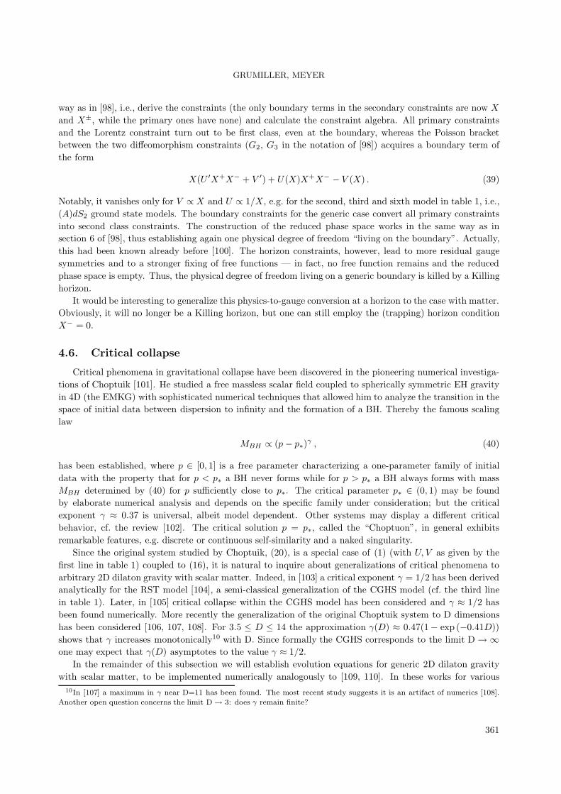
X(U ′X+X− + V ′) + U(X)X+X− − V (X) . (39)

Notably, it vanishes only for V ∝ X and U ∝ 1/X, e.g. for the second, third and sixth model in table 1, i.e.,(A)dS2 ground state models. The boundary constraints for the generic case convert all primary constraintsinto second class constraints. The construction of the reduced phase space works in the same way as insection 6 of [98], thus establishing again one physical degree of freedom “living on the boundary”. Actually,this had been known already before [100]. The horizon constraints, however, lead to more residual gaugesymmetries and to a stronger fixing of free functions — in fact, no free function remains and the reducedphase space is empty. Thus, the physical degree of freedom living on a generic boundary is killed by a Killinghorizon.

It would be interesting to generalize this physics-to-gauge conversion at a horizon to the case with matter.Obviously, it will no longer be a Killing horizon, but one can still employ the (trapping) horizon conditionX− = 0.

4.6. Critical collapse

Critical phenomena in gravitational collapse have been discovered in the pioneering numerical investiga-tions of Choptuik [101]. He studied a free massless scalar field coupled to spherically symmetric EH gravityin 4D (the EMKG) with sophisticated numerical techniques that allowed him to analyze the transition in thespace of initial data between dispersion to infinity and the formation of a BH. Thereby the famous scalinglaw

MBH ∝ (p − p∗)γ , (40)

has been established, where p ∈ [0, 1] is a free parameter characterizing a one-parameter family of initialdata with the property that for p < p∗ a BH never forms while for p > p∗ a BH always forms with massMBH determined by (40) for p sufficiently close to p∗. The critical parameter p∗ ∈ (0, 1) may be foundby elaborate numerical analysis and depends on the specific family under consideration; but the criticalexponent γ ≈ 0.37 is universal, albeit model dependent. Other systems may display a different criticalbehavior, cf. the review [102]. The critical solution p = p∗, called the “Choptuon”, in general exhibitsremarkable features, e.g. discrete or continuous self-similarity and a naked singularity.

Since the original system studied by Choptuik, (20), is a special case of (1) (with U, V as given by thefirst line in table 1) coupled to (16), it is natural to inquire about generalizations of critical phenomena toarbitrary 2D dilaton gravity with scalar matter. Indeed, in [103] a critical exponent γ = 1/2 has been derivedanalytically for the RST model [104], a semi-classical generalization of the CGHS model (cf. the third linein table 1). Later, in [105] critical collapse within the CGHS model has been considered and γ ≈ 1/2 hasbeen found numerically. More recently the generalization of the original Choptuik system to D dimensionshas been considered [106, 107, 108]. For 3.5 ≤ D ≤ 14 the approximation γ(D) ≈ 0.47(1− exp (−0.41D))shows that γ increases monotonically10 with D. Since formally the CGHS corresponds to the limit D→ ∞one may expect that γ(D) asymptotes to the value γ ≈ 1/2.

In the remainder of this subsection we will establish evolution equations for generic 2D dilaton gravitywith scalar matter, to be implemented numerically analogously to [109, 110]. In these works for various

10In [107] a maximum in γ near D=11 has been found. The most recent study suggests it is an artifact of numerics [108].

Another open question concerns the limit D→ 3: does γ remain finite?

361

GRUMILLER, MEYER

reasons Sachs-Bondi gauge has been used. Thus we employ

e+0 = 0 , e−0 = 1 , x0 = X , (41)

while the remaining Zweibein components are parameterized as

e−1 = α(u,X) , e+1 = I(X)e2β(u,X) . (42)

In the gauge (41) with the parameterization (42) the line element reads

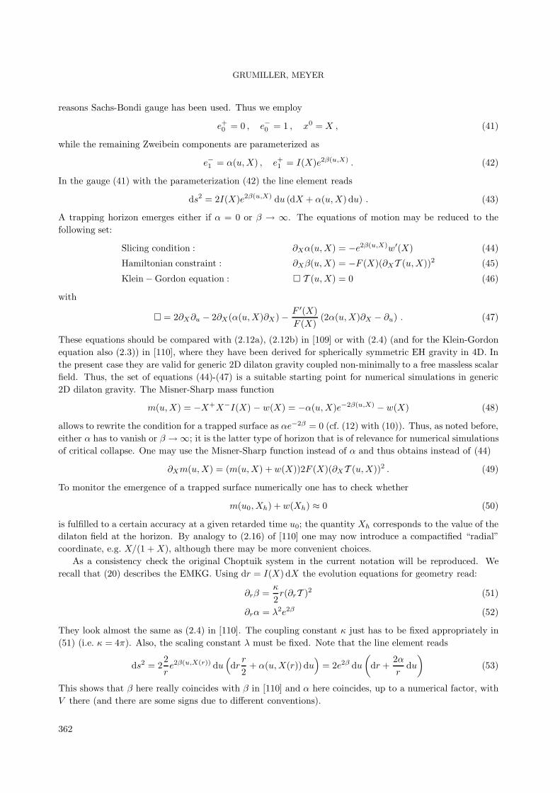
ds2 = 2I(X)e2β(u,X) du (dX + α(u,X) du) . (43)

A trapping horizon emerges either if α = 0 or β → ∞. The equations of motion may be reduced to thefollowing set:

Slicing condition : ∂Xα(u,X) = −e2β(u,X)w′(X) (44)

Hamiltonian constraint : ∂Xβ(u,X) = −F (X)(∂XT (u,X))2 (45)

Klein−Gordon equation : T (u,X) = 0 (46)

with

= 2∂X∂u − 2∂X(α(u,X)∂X)− F ′(X)F (X)

(2α(u,X)∂X − ∂u) . (47)

These equations should be compared with (2.12a), (2.12b) in [109] or with (2.4) (and for the Klein-Gordonequation also (2.3)) in [110], where they have been derived for spherically symmetric EH gravity in 4D. Inthe present case they are valid for generic 2D dilaton gravity coupled non-minimally to a free massless scalarfield. Thus, the set of equations (44)-(47) is a suitable starting point for numerical simulations in generic2D dilaton gravity. The Misner-Sharp mass function

m(u,X) = −X+X−I(X) − w(X) = −α(u,X)e−2β(u,X) − w(X) (48)

allows to rewrite the condition for a trapped surface as αe−2β = 0 (cf. (12) with (10)). Thus, as noted before,either α has to vanish or β →∞; it is the latter type of horizon that is of relevance for numerical simulationsof critical collapse. One may use the Misner-Sharp function instead of α and thus obtains instead of (44)

∂Xm(u,X) = (m(u,X) +w(X))2F (X)(∂XT (u,X))2 . (49)

To monitor the emergence of a trapped surface numerically one has to check whether

m(u0, Xh) +w(Xh) ≈ 0 (50)

is fulfilled to a certain accuracy at a given retarded time u0; the quantity Xh corresponds to the value of thedilaton field at the horizon. By analogy to (2.16) of [110] one may now introduce a compactified “radial”coordinate, e.g. X/(1 + X), although there may be more convenient choices.

As a consistency check the original Choptuik system in the current notation will be reproduced. Werecall that (20) describes the EMKG. Using dr = I(X) dX the evolution equations for geometry read:

∂rβ =κ

2r(∂rT )2 (51)

∂rα = λ2e2β (52)

They look almost the same as (2.4) in [110]. The coupling constant κ just has to be fixed appropriately in(51) (i.e. κ = 4π). Also, the scaling constant λ must be fixed. Note that the line element reads

ds2 = 22re2β(u,X(r)) du

(drr

2+ α(u,X(r)) du

)= 2e2β du

(dr +

2αr

du)

(53)

This shows that β here really coincides with β in [110] and α here coincides, up to a numerical factor, withV there (and there are some signs due to different conventions).

362

GRUMILLER, MEYER

4.7. Quasinormal modes

The term “quasinormal modes” refers to some set of modes with a complex frequency, associated withsmall perturbations of a BH. For U = 0 and monomial V in [111] quasinormal modes arising from a scalarfield, (16) with f = 0 and F ∝ Xp, have been studied in the limit of high damping by virtue of the“monodromy approach”, and the relation

eω/TH = −(1 + 2 cos (π(1− p))) (54)

for the frequency ω has been found (TH is Hawking temperature as defined in (34)). Minimally coupledscalar fields (p = 0) lead to the trivial result ω/TH = 2πin. High damping implies that the integer n has tobe large. For the important case of p = 1 (relevant for the first and fifth entry in table 1) one obtains from(54)

ω

TH= 2πi

(n+

12

)+ ln 3 . (55)

The result (55) coincides with the one obtained for the Schwarzschild BH with 4D methods, both numerically[112] and analytically [113]. Moreover, consistency with D > 4 is found as well [114]. This shows that the2D description of BHs is reliable also with respect to highly damped quasinormal modes.

4.8. Solid state analogues

BH analogues in condensed matter systems go back to the seminal paper by Unruh [115]. Due to theamazing progress in experimental condensed matter physics, in particular Bose-Einstein condensates, in thepast decade the subject of BH analogues has flourished, cf. e.g. [116] and references therein.

In some cases the problem effectively reduces to 2D. It is thus perhaps not surprising that an analoguesystem for the Jackiw-Teitelboim model has been found [117] for a cigar shaped Bose-Einstein condensate.More recently this has led to some analogue 2D activity [118]. Note, however, that some issues, like theone of backreaction, might not be modelled very well by an effective action method [119]. Indeed, 2Ddilaton gravity with matter could be of interest in this context, because these systems might allow notjust kinematical but dynamical equivalence, i.e., not only the fluctuations (e.g. phonons) behave as thecorresponding gravitational ones (e.g. Hawking quanta), but also the background dynamics does (e.g. theflow of the fluid or the metric, respectively). Such a system would be a necessary pre-requisite to studyissues of mass and entropy in an analogue context. At least for static solutions this is possible [120], but ofcourse the non-static case would be much more interesting. Alas, it is not only more interesting but alsoconsiderably more difficult, and a priori there is no reason why one should succeed in finding a fully fledgedanalogue model of 2D dilaton gravity with matter. Still, one can hope and try.

5. Geometry from matter

In first order gravity (3) coupled to scalar (16) or fermionic (17) matter the geometry can be quantizedexactly: after analyzing the constraints, fixing EF gauge

(ω0, e−0 , e+0 ) = (0, 1, 0) (56)

and constructing a BRST invariant Hamiltonian, the path integral can be evaluated exactly and a (nonlocal)effective action is obtained [121]. Subsequently the matter fields can be quantized by means of ordinaryperturbation theory. To each order all backreactions are included automatically by this procedure.

Although geometry has been integrated out exactly, it can be recovered off-shell in the form of interac-tion vertices of the matter fields, some of which resemble virtual black holes (VBHs) [122, 123, 15]. This

363

GRUMILLER, MEYER

i0

i-

i+

ℑ-

ℑ+

y

Figure 2. VBH

metamorphosis of geometry however does not take place in the matterless case [124], where the quantumeffective action coincides with the classical action in EF gauge. We hasten to add that one should not takethis off-shell geometry at face value — this would be like over-interpreting the role of virtual particles in aloop diagram. But the simplicity of such geometries and the fact that all possible configurations are summedover are both nice qualitative features of this picture.

A Carter-Penrose diagram of a typical VBH configuration is depicted in figure 2. The curvature scalarof such effective geometries is discontinuous and even has a δ-peak. A typical effective line element (for theEMKG) reads

(ds)2 = 2 dr du+(

1− θ(ry − r)δ(u − uy)(

2mr

+ ar − d))

(du)2 , (57)

It obviously has a Schwarzschild part with ry-dependent “mass” m and a Rindler part with ry-dependent“acceleration” a, both localized on a lightlike cut. This geometry is nonlocal in the sense that it dependsnot just on the coordinates r, u but additionally on a second point ry, uy. While the off-shell geometry (57)is highly gauge dependent, the ensuing S-matrix — the only physical observable in this context [125] —appears to be gauge independent, although a formal proof of this statement, e.g. analogously to [126], islacking.

5.1. Scalar matter

After integrating out geometry and the ghost sector (for f(X, T ) = 0), the effective Lagrangian (w isdefined in (4))

LeffT = F (X)(∂0T )(∂1T )− w′(X) + sources (58)

contains the quantum version of the dilaton field X = X(∇−20 (∂0T )2), depending non-locally on T . The

quantity X solves the equation of motion of the classical dilaton field, with matter terms and external sourcesfor the geometric variables in EF gauge. The simplicity of (58) is in part due to the gauge choice (56) andin part due to the linearity of the gauge fixed Lagrangian in the remaining gauge field components, thusproducing delta-functionals upon path integration.

In principle, the interaction vertices can be extracted by expanding the nonlocal effective action in apower series of the scalar field T . However, this becomes cumbersome already at the T 4 level. Fortu-nately, the localization technique introduced in [121] simplifies the calculations considerably. It relies on

364

GRUMILLER, MEYER

V(4)(x,y)a

x y

∂0 S

q’

∂0 S

q

∂0 S

k’

∂0 S

k

+

V(4)(x,y)b

x y

∂0 S

q’

∂0 S

q

∂1 S

k’

∂0 S

k

Figure 3. Non-local 4-point vertices

two observations: First, instead of dealing with complicated nonlocal kernels one may solve correspondingdifferential equations after imposing asymptotic conditions on the solutions. Second, instead of taking then-th functional derivative of the action with respect to bilinear combinations of T , the matter fields may belocalized at n different space-time points, which mimics the effect of functional differentiation. For tree-levelcalculations it is then sufficient to solve the classical equations of motion in the presence of these sources,which is achieved most easily via appropriate matching conditions.

It turns out (as anticipated from (57)) that the conserved quantity (10) is discontinuous for a VBH. Thisphenomenon is generic [15].11 The corresponding Feynman diagrams are contained in figure 3.12 For free,massless, non-minimally coupled scalars (F = const.) both the symmetric and the non-symmetric 4-pointvertex

V (4) =∫

d2x d2y(∂0T )2x[Va(x, y)(∂0T )2y + Vb(x, y)(∂0T )y(∂1T )y

](59)

are given in [15], and have the following properties:

1. They are local in one coordinate (e.g. containing δ(x1 − y1)) and nonlocal in the other.

2. They vanish in the local limit (x0 → y0). Additionally, Vb vanishes for minimal coupling F = const.

3. The symmetric vertex depends only on the conformal invariant combination w(X) and the asymptoticvalue M∞ of (10). The non-symmetric one is independent of U , V and M∞. Thus if M∞ is fixed inall conformal frames, both vertices are conformally invariant.

4. They respect the Z2 symmetry F (X) → −F (X).

It should be noted that the class of models with UV + V ′ = 0 and F = const (containing the CGHS model,the seventh and eleventh entry in table 1) shows “scattering triviality”, i.e., the classical vertices vanish,and scattering can only arise from higher order quantum backreactions. For these models the VBH has noclassically observable consequences, but at 1-loop level physical observables like the specific heat are modifiedappreciably [127].

The 2D Klein-Gordon equation relevant for the construction of asymptotic states is also conformallyinvariant. For minimal coupling it simplifies considerably, and a complete set of asymptotic states can beobtained explicitly. Since both, asymptotic states and vertices, only depend on w(X) and M∞, at tree levelconformal invariance holds nonperturbatively (to all orders in T ), but it is broken at 1-loop level due tothe conformal anomaly. Because asymptotically geometry does not fluctuate, a standard Fock space may bebuilt with creation/annihilation operators a±(k) obeying the standard commutation relations. The S-matrixfor two ingoing (q, q′) into two outgoing (k, k′) asymptotic modes is determined by (cf. (59))

T (q, q′; k, k′) =12〈0∣∣∣a−(k)a−(k′)V (4)a+(q)a+(q′)

∣∣∣ 0〉 . (60)

11With the exception of scattering trivial models, cf. the eleventh entry in table 1.12The scalar field T is denoted by S in these graphs.

365

GRUMILLER, MEYER

The simple choice M∞ = 0 yields a “standard QFT vacuum” |0〉, provided the model under considerationhas a Minkowskian ground state (e.g. the first, third, fifth and last model in table 1).

For the physically interesting case of the EMKG model such an S-matrix was obtained in [128, 123].Both the symmetric and the non-symmetric vertex contribute, each giving a divergent contribution to theS-matrix, but the sum of both turned out to be finite! The whole calculation is highly nontrivial, involvingcancellations of polylogarithmic terms, but at the end giving the surprisingly simple result

T (q, q′; k, k′) = − iκδ (k + k′ − q − q′)2(4π)4|kk′qq′|3/2 E3T , (61)

with ingoing (q, q′) and outgoing (k, k′) spatial momenta, total energy E = q + q′,

T :=1E3

[Π ln

Π2

E6+

1Π

∑p∈k,k′,q,q′

p2 lnp2

E2·(

3kk′qq′ − 12

∑r =p

∑s =r,p

(r2s2

))], (62)

and the momentum transfer function Π = (k + k′)(k − q)(k′ − q). The factor T is invariant under rescalingof the momenta p → ap, and the whole amplitude transforms monomial like T → a−4T . It should be notedthat due to the non-locality of the vertices there is just one δ-function of momentum conservation (but noseparate energy conservation) present in (61). This is advantageous because it eliminates the problem of“squared δ-functions” that is otherwise present in 2D theories of massless scalar fields (cf. e.g. [129]). In thissense gravity acts as a regulator of the theory.

The corresponding differential cross section also reveals interesting features [123]:

1. For vanishing Π forward scattering poles are present.

2. There is an approximate self-similarity close to the forward scattering peaks. Far away from them itis broken, however.

3. It is CPT invariant.

4. An ingoing s-wave can decay into three outgoing ones. Although this may be expected on generalgrounds, within the present formalism it is possible to provide explicit results for the decay rate.

Although it seems straightforward to generalize (60) to arbitrary n-point vertices, no such calculation hasbeen attempted so far. This is related to the fact that the derivation of (61) has been somewhat tediousand lengthy. Thus, it could be worthwhile to find a more efficient way to obtain this interesting S-matrixelement.

5.2. Fermionic matter

Recently we considered 2D dilaton gravity (3) coupled to fermions (17) along the lines of the previoussubsection. The results will be published elsewhere, but we give a short summary with emphasis on differencesto the scalar case.

The constraint analysis for the general case (17) has been worked out first in [42]. Three first classconstraints generating the two diffeomorphisms and the local Lorentz symmetry and four well-known secondclass constraints relating the four real components of the Dirac spinor to their canonical momenta are presentin the system. As anticipated the Hamiltonian is fully constrained. After introducing the Dirac bracket theconstructions of the BRST charge and the gauge fixed Hamiltonian are straightforward. Path integrationover geometry is even simpler than in the scalar case, because the second class constraints are implementedin the path integral through delta functionals, allowing to integrate out the fermion momenta. The effective

366

GRUMILLER, MEYER

Lagrangian

Leffχ =i√2F (X)(χ∗

1←→∂1 χ1)

+I(X)(

i√2F (X)(χ∗

0←→∂0 χ0) + H(X)g(χχ)− V (X)

)+ sources (63)

again depends on the quantum version X = X(∇−20 (χ∗

1←→∂0 χ1)) of the dilaton field and exhibits non-locality

in the matter field.

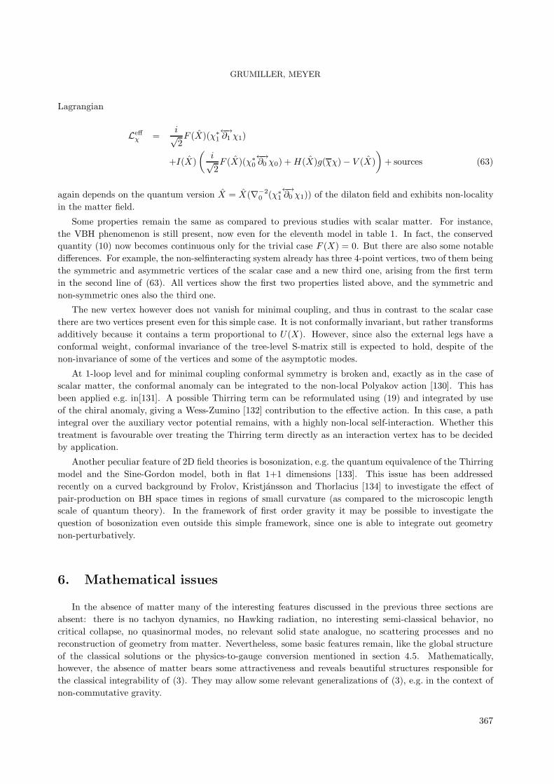
Some properties remain the same as compared to previous studies with scalar matter. For instance,the VBH phenomenon is still present, now even for the eleventh model in table 1. In fact, the conservedquantity (10) now becomes continuous only for the trivial case F (X) = 0. But there are also some notabledifferences. For example, the non-selfinteracting system already has three 4-point vertices, two of them beingthe symmetric and asymmetric vertices of the scalar case and a new third one, arising from the first termin the second line of (63). All vertices show the first two properties listed above, and the symmetric andnon-symmetric ones also the third one.

The new vertex however does not vanish for minimal coupling, and thus in contrast to the scalar casethere are two vertices present even for this simple case. It is not conformally invariant, but rather transformsadditively because it contains a term proportional to U(X). However, since also the external legs have aconformal weight, conformal invariance of the tree-level S-matrix still is expected to hold, despite of thenon-invariance of some of the vertices and some of the asymptotic modes.

At 1-loop level and for minimal coupling conformal symmetry is broken and, exactly as in the case ofscalar matter, the conformal anomaly can be integrated to the non-local Polyakov action [130]. This hasbeen applied e.g. in[131]. A possible Thirring term can be reformulated using (19) and integrated by useof the chiral anomaly, giving a Wess-Zumino [132] contribution to the effective action. In this case, a pathintegral over the auxiliary vector potential remains, with a highly non-local self-interaction. Whether thistreatment is favourable over treating the Thirring term directly as an interaction vertex has to be decidedby application.

Another peculiar feature of 2D field theories is bosonization, e.g. the quantum equivalence of the Thirringmodel and the Sine-Gordon model, both in flat 1+1 dimensions [133]. This issue has been addressedrecently on a curved background by Frolov, Kristjansson and Thorlacius [134] to investigate the effect ofpair-production on BH space times in regions of small curvature (as compared to the microscopic lengthscale of quantum theory). In the framework of first order gravity it may be possible to investigate thequestion of bosonization even outside this simple framework, since one is able to integrate out geometrynon-perturbatively.

6. Mathematical issues

In the absence of matter many of the interesting features discussed in the previous three sections areabsent: there is no tachyon dynamics, no Hawking radiation, no interesting semi-classical behavior, nocritical collapse, no quasinormal modes, no relevant solid state analogue, no scattering processes and noreconstruction of geometry from matter. Nevertheless, some basic features remain, like the global structureof the classical solutions or the physics-to-gauge conversion mentioned in section 4.5. Mathematically,however, the absence of matter bears some attractiveness and reveals beautiful structures responsible forthe classical integrability of (3). They may allow some relevant generalizations of (3), e.g. in the context ofnon-commutative gravity.

367

GRUMILLER, MEYER

6.1. Remarks on the Einstein-Hilbert action in 2D

In 2D the Einstein tensor vanishes identically for any 2D metric and thus conveys no useful information.Similarly, the 2D EH action, supplemented appropriately by boundary and corner terms, just counts thenumber of holes of a compact Riemannian manifold, cf. e.g. [135]. Thus, as compared to (1) or (3) the studyof “pure” 2D gravity, i.e., without coupling to a dilaton field, is of rather limited interest. If one adds acosmological constant term one may study quantum gravity in 2D by means of dynamical triangulations,cf. e.g. [136] and references therein. The EH part of the action plays no essential role, however.

It is possible to consider EH gravity in 2 + ε dimensions, an idea which seems to go back to [137]. Aftertaking the limit ε → 0 in a specific way [138] one obtains again a dilaton gravity model (1) with V = 0and U = const. (cf. the eleventh model in table 1). That such a limit can be very subtle has been shownrecently by Jackiw [139] in the context of Weyl invariant scalar field dynamics: if one simply drops the EHterm in equation (3.5) of that work the Liouville model is obtained (cf. the tenth model in table 1), butWeyl invariance is lost.

6.2. Relations to 3D: Chern-Simons and BTZ

The gravitational Chern-Simons term [140] and the 3D BTZ BH [141] have inspired a lot of furtherresearch. Here we will focus on relations to (1) and (3): dimensional reduction of the BTZ to 2D has beenperformed in [19], cf. the fifteenth model in table 1. A reduction of the gravitational Chern-Simons termfrom 3D to 2D has been performed in [20], cf. the sixteenth model in table 1. Recently [142], such reductionshave been exploited to calculate the entropy of a BTZ BH in the presence of gravitational Chern-Simonsterms, something which is difficult to achieve in 3D because there is no manifestly covariant formulationof the Chern-Simons term, whereas the reduced theory is manifestly covariant. It is not unlikely that alsoother open problems of 3D gravity may be tackled with 2D methods.

6.3. Integrable systems, Poisson-sigma models and KdV surfaces

Some of the pioneering work has been mentioned already in section 2.1 and in table 1. In two seminalpapers by Kummer and Schwarz [143] the usefulness of light-cone gauge for the Lorentz frame and EF gaugefor the curved metric has been demonstrated for the fourteenth model in table 1, which is a rather genericone as it has non-vanishing U and non-monomial V . A Hamiltonian analysis [72] revealed an interesting(W-)algebraic structure of the secondary constraints together with the fields X,X± as generators. Thecenter of this algebra consists of the conserved quantity (10) and its first derivative, ∂1M (which, of course,vanishes on the surface of constraints). Consequently, it has been shown by Schaller and Strobl [31] that (3)is a special case of a Poisson-sigma model,13

SPSM = −∫M

[XI dAI −

12P IJAJ ∧AI

], (64)

with a 3D target space, the coordinates of which are XI = X,X+, X−. The gauge fields comprise theCartan variables, AI = ω, e−, e+. Because the dimension of the Poisson manifold is odd the Poisson tensor(I, J ∈ X,±)

PX± = ±X± , P+− = X+X−U(X) + V (X) , P IJ = −P JI , (65)

cannot have full rank. Therefore, always a Casimir function, (10), exists, which may be interpreted as“mass”. Note that (65) indeed fulfills the required Jacobi-identities, P IL∂LP

JK + perm (IJK) = 0. For ageneric (graded) Poisson-sigma model (64) the commutator of two symmetry transformations

δXI = P IJεJ , δAI = −dεI −(∂IP

JK)εK AJ , (66)

13Dirac-sigma models [144] are a recent generalization thereof.

368

GRUMILLER, MEYER

is a (non-linear) symmetry modulo the equations of motion. Only for P IJ linear in XI a Lie algebra isobtained; cf. the second model in table 1. For (65) the symmetries (66) on-shell correspond to local Lorentztransformations and diffeomorphisms. Generalizations discussed in section 2.4 are particularly transparentin this approach; essentially, one has to add more target space coordinates to the Poisson manifold, some ofwhich will be fermionic in supergravity extensions, cf. e.g. [39].

Actually, there exist various approaches to integrability of gravity models in 2D, cf. e.g. [145], and wecan hardly do them justice here. We will just point out a relation to Korteweg-de Vries (KdV) surfacesas discussed recently in [146]. These are 2D surfaces embedded in 3D Minkowski space arising from theKdV equation ∂tw = ∂3xw + 6w∂xw, with line element (cf. (11) in [146]; u there coincides with w here)ds2 = 2 dX du− (4λ−w(X, u)) du2, where X ∝ x, u ∝ t and λ is some constant. For static KdV solutions,∂uw = 0, this line element is also a solution of (3) as can bee seen from (11), with λ playing the role of themass M . In the non-static case it describes a solution of (3) coupled to some energy-momentum tensor. Itcould be of interest to pursue this relation in more depth.

6.4. Torsion and non-metricity

For U = 0 the equation of motion R = 2V ′(X), if invertible, allows to rewrite the action (1) as SR =∫d2x√−gf(R), cf. e.g. [147] and references therein. As compared to such theories, the literature on models

with torsion τa = ∗T a,

SRT =∫

d2x√−gf(R, τaτa) , (67)

is relatively scarce and consists mainly of elaborations based upon the fourteenth model in table 1, wheref = Aτaτa +BR2 + CR+ Λ, also known as “Poincare gauge theory”, cf. [148] and references therein. Thismodel in particular (and a large class of models of type (67)) allows an equivalent reformulation as (3).Thus, they need not be discussed separately.

A generalization which includes also effects from non-metricity has been studied in [149]. Elimination ofnon-metricity leads again to models of type (1), (3), but one has to be careful with such reformulations astest-particles moving along geodesics or, alternatively, along auto-parallels, may “feel” the difference. Thus,it could be of interest to generalize (3) (which already contains torsion if U = 0) as to include non-metricity,thus dropping the requirement that the connection ωa

b is proportional to εab. However, a formulation asPoisson-sigma model (64) (with 6D target space) seems to be impossible as there are only trivial solutionsto the Jacobi identities.

6.5. Non-commutative gravity

In the 1970ies/1980ies theories have been supersymmetrized, in the 1990ies/2000s theories have been“non-commutativized”, for reviews cf. e.g. [150]. The latter procedure still has not stopped as the originalidea, namely to obtain a fully satisfactory non-commutative version of gravity, has not been achieved so far.In order to get around the main conceptual obstacles it is tempting to consider the simplified framework of2D.

There it is possible to construct non-commutative dilaton gravity models with a usual (non-twisted)realization of gauge symmetries.14 A non-commutative version of the Jackiw-Teitelboim model (cf. thesecond entry in table 1),

SNCJT = −12

∫d2x εµν

[Xa D T

aµν +Xab D

(Rab

µν − Λeaµ D ebν

)], (68)

14Another approach has been pursued in [151].

369

GRUMILLER, MEYER

has been constructed in [152] and then quantized in [153]. A non-commutative version of the fourth model intable 1 was suggested in [154]. For a definition of the Moyal-D and further notation cf. these two references.A crucial change as compared to (3), besides the D, is the appearance of a second dilaton field ψ in 2Xab =Xεab − iψηab. However, interesting as these results may be, there seems to be no way to generalize them togeneric 2D dilaton gravity without twisting the gauge symmetries [155]. Moreover, the fact that the metriccan be changed by “Lorentz transformations” seems questionable from a physical point of view, cf. [156] fora similar problem.

An important step towards constructing a satisfactory non-commutative gravity was recently made byWess and collaborators [157], who understood how one can construct diffeomorphism invariants, includingthe EH action, on non-commutative spaces (see also [158] for a real formulation). There is, however, a priceto pay. The diffeomorphism group becomes twisted, i.e., there is a non-trivial coproduct [159]. Recently itcould be shown [160] that twisted gauge symmetries close for arbitrary gauge groups and thus a constructionof twisted-invariant actions is straightforward. The main element in that construction (cf. also [159, 161,157, 158] and [162]) is the twist operator

F = expP, P =i

2θµν∂µ ⊗ ∂ν , (69)

which acts on the tensor products of functions φ1 ⊗ φ2. With the multiplication map µ(φ1 ⊗ φ2) = φ1 · φ2and (69) the Moyal-Weyl representation of the star product,

φ1 D φ2 = µ F(φ1 ⊗ φ2) = µ*(φ1 ⊗ φ2) , (70)

can be constructed. Consider now generators u of some symmetry transformations which form a Lie algebra.If one knows the action of these transformations on primary fields, δuφ = uφ, the action on tensor productsis defined by the coproduct ∆. In the undeformed case the coproduct is primitive, ∆0(u) = u ⊗ 1 + 1 ⊗ u

and δu(φ1 ⊗ φ2) = ∆0(u)(φ1 ⊗ φ2) = uφ1 ⊗ φ2 + φ1 ⊗ uφ2 satisfies the usual Leibniz rule. The action ofsymmetry generators on elementary fields is left undeformed, but the coproduct is twisted,

∆(u) = exp(−P)∆0(u) exp(P) . (71)

Obviously, twisting preserves the commutation relations. Therefore, the commutators of gauge transforma-tions for an arbitrary gauge group close.

It seems plausible that a corresponding generalization to twisted non-linear gauge symmetries willbe a crucial technical pre-requisite to a successful construction of generic non-commutative 2D dilatongravity[164].15 It would allow, among other things, a thorough discussion of non-commutative BHs, alongthe lines of sections 2-5.

Acknowledgments

DG and RM would like to thank cordially L. Bergamin, W. Kummer and D. Vassilevich for a long-timecollaboration and helpful discussions, respectively, on most of the topics reviewed in this work. Moreover,DG is grateful to M. Adak, P. Aichelburg, S. Alexandrov, H. Balasin, M. Bojowald, M. Cadoni, S. Car-lip, T. Dereli, M. Gurses, A. Iorio, R. Jackiw, M. Katanaev, C. Lechner, F. Meyer, S. Mignemi, C. Nunez,Y. Obukhov, M.-I. Park, M. Purrer, R. Schutzhold, T. Strobl, W. Unruh, P. van Nieuwenhuizen and S. Wein-furtner for helpful discussions and/or correspondence. In addition, DG would like to thank the organizers ofthe Fifth Workshop on QUANTIZATION, DUALITIES AND INTEGRABLE SYSTEMS in Denizli, Turkey,in particular M. Adak for the kind invitation.

DG has been supported by project GR-3157/1-1 of the German Research Foundation (DFG). Additionalfinancial support due to Pamukkale University is acknowledged gratefully. RM has been supported financiallyby the MPI and expresses his gratitude to J. Jost in this regard.

15The relation of (64) to a specific Lie algebroid [163] could be helpful in this context.

370

GRUMILLER, MEYER

References

[1] Such a life, with all vision limited to a Point, and all motion to a Straight Line, seemed to me inexpressibly

dreary; and I was surprised to note the vivacity and cheerfulness of the King. [Edwin A. Abbot, “Flatland —

A Romance of Many Dimensions.” Dover Publications 1992, New York. (first published under the pseudonym

A. Square in 1884, Seeley & Co., London)].

[2] J. Brown, Lower Dimensional Gravity. World Scientific, 1988.

[3] A. M. Polyakov, Mod. Phys. Lett., A2, (1987), 893.

[4] D. Grumiller, W. Kummer, and D. V. Vassilevich, Phys. Rept., 369, (2002), 327, hep-th/0204253.

[5] P. Thomi, B. Isaak, and P. Hajicek, Phys. Rev., D30, (1984), 1168.

P. Hajicek, Phys. Rev., D30, (1984), 1178.

[6] C. Teitelboim, Phys. Lett., B126, (1983), 41.

[7] R. Jackiw, Nucl. Phys., B252, (1985), 343.

[8] E. Witten, Phys. Rev., D44, (1991), 314.

G. Mandal, A. M. Sengupta, and S. R. Wadia, Mod. Phys. Lett., A6, (1991), 1685.

S. Elitzur, A. Forge, and E. Rabinovici, Nucl. Phys., B359, (1991), 581.

[9] C. G. Callan, Jr., S. B. Giddings, J. A. Harvey, and A. Strominger, Phys. Rev., D45, (1992), 1005,

hep-th/9111056.

[10] J. P. S. Lemos and P. M. Sa, Phys. Rev., D49, (1994), 2897, arXiv:gr-qc/9311008.

[11] A. Fabbri and J. G. Russo, Phys. Rev., D53, (1996), 6995, hep-th/9510109.

[12] D. Grumiller, JCAP, 05, (2004), 005, gr-qc/0307005.

[13] M. O. Katanaev, W. Kummer, and H. Liebl, Nucl. Phys., B486, (1997), 353, gr-qc/9602040.

[14] Y. Nakayama, Int. J. Mod. Phys., A19, (2004), 2771, hep-th/0402009.

[15] D. Grumiller, W. Kummer, and D. V. Vassilevich, European Phys. J., C30, (2003), 135, hep-th/0208052.

[16] H. Reissner, Ann. Phys., 50, (1916), 106.

G. Nordstrom, Proc. Kon. Ned. Akad. Wet., 20, (1916), 1238.

[17] S. W. Hawking and D. N. Page, Commun. Math. Phys., 87, (1983), 577.

[18] M. O. Katanaev and I. V. Volovich, Phys. Lett., B175, (1986), 413; Ann. Phys., 197, (1990), 1.

[19] A. Achucarro and M. E. Ortiz, Phys. Rev., D48, (1993), 3600, hep-th/9304068.

[20] G. Guralnik, A. Iorio, R. Jackiw, and S. Y. Pi, Ann. Phys., 308, (2003), 222, hep-th/0305117.

[21] D. Grumiller and W. Kummer, Ann. Phys., 308, (2003), 211, hep-th/0306036.

L. Bergamin, D. Grumiller, A. Iorio, and C. Nunez, JHEP, 11, (2004), 021, hep-th/0409273.

[22] L. Bergamin, hep-th/0509183.

[23] M. R. Douglas et al., hep-th/0307195.

[24] S. Gukov, T. Takayanagi, and N. Toumbas, JHEP, 03, (2004), 017, hep-th/0312208.

[25] R. Dijkgraaf, H. Verlinde, and E. Verlinde, Nucl. Phys., B371, (1992), 269.

371

GRUMILLER, MEYER

[26] D. Grumiller, JHEP, 05, (2005), 028, hep-th/0501208.

[27] K. Isler and C. A. Trugenberger, Phys. Rev. Lett., 63, (1989), 834.

A. H. Chamseddine and D. Wyler, Phys. Lett., B228, (1989), 75.

[28] H. Verlinde, in Trieste Spring School on Strings and Quantum Gravity, p. 178. April, 1991. the same lectures

have been given at MGVI in Japan, June, 1991.

[29] D. Cangemi and R. Jackiw, Phys. Rev. Lett., 69, (1992), 233, hep-th/9203056.

A. Achucarro, Phys. Rev. Lett., 70, (1993), 1037, hep-th/9207108.

[30] N. Ikeda and K. I. Izawa, Prog. Theor. Phys., 90, (1993), 237, hep-th/9304012.

[31] P. Schaller and T. Strobl, Mod. Phys. Lett., A9, (1994), 3129, hep-th/9405110.

[32] J. G. Russo and A. A. Tseytlin, Nucl. Phys., B382, (1992), 259, arXiv:hep-th/9201021.

S. D. Odintsov and I. L. Shapiro, Phys. Lett., B263, (1991), 183.

T. Banks and M. O’Loughlin, Nucl. Phys., B362, (1991), 649.

R. B. Mann, A. Shiekh, and L. Tarasov, Nucl. Phys., B341, (1990), 134.

[33] T. Klosch and T. Strobl, Class. Quant. Grav., 13, (1996), 2395, arXiv:gr-qc/9511081.

[34] T. Klosch and T. Strobl, Class. Quant. Grav., 13, (1996), 965, arXiv:gr-qc/9508020.

[35] J.-G. Hao and X.-Z. Li, Phys. Rev., D68, (2003), 083514, hep-th/0306033.

[36] L. Bergamin, D. Grumiller, and W. Kummer, J. Phys., A37 (2004), 3881, hep-th/0310006.

[37] D. M. Thompson, Phys. Rev., D70, (2004), 106001, hep-th/0312156.

[38] D. Birmingham, M. Blau, M. Rakowski, and G. Thompson, Phys. Rept., 209, (1991), 129.

[39] T. Strobl, hep-th/0011240. Habilitation thesis.

[40] Y.-C. Park and A. Strominger, Phys. Rev., D47, (1993), 1569, arXiv:hep-th/9210017.

J. M. Izquierdo, Phys. Rev., D59, (1999), 084017, arXiv:hep-th/9807007.

T. Strobl, Phys. Lett., B460, (1999), 87, arXiv:hep-th/9906230.

M. Ertl, W. Kummer, and T. Strobl, JHEP, 01, (2001), 042, arXiv:hep-th/0012219.

M. Ertl, PhD thesis, Technische Universitat Wien, 2001. arXiv:hep-th/0102140.

L. Bergamin and W. Kummer, Phys. Rev., D68, (2003), 104005, hep-th/0306217; Eur. Phys. J., C39,

(2005), 41, hep-th/0402138; Eur. Phys. J., C39, (2005), S53, hep-th/0411204.

L. Bergamin, D. Grumiller, and W. Kummer, JHEP, 05, (2004), 060, hep-th/0404004.

[41] L. Bergamin and W. Kummer, JHEP, 05, (2003), 074, hep-th/0209209.

[42] R. Meyer, hep-th/0512267.

[43] W. E. Thirring, Annals Phys., 3, (1958), 91.

[44] H. Balasin, C. G. Boehmer, and D. Grumiller, Gen. Rel. Grav., 37, (2005), 1435, gr-qc/0412098.

[45] W. Kummer, HADRON STRUCTURE ’92, D. Bruncko and J. Urban, eds. September, 1992. Stara Lesna,

Czechoslovakia.

[46] H. Pelzer and T. Strobl, Class. Quant. Grav., 15, (1998), 3803, arXiv:gr-qc/9805059.

[47] P. C. Aichelburg and R. U. Sexl, Gen. Rel. Grav., 2, (1971), 303.

372

GRUMILLER, MEYER

[48] H. Balasin and D. Grumiller, Class. Quant. Grav., 21, (2004), 2859, gr-qc/0312086.

[49] I. Z. Fisher, Zh. Eksp. Teor. Fiz., 18, (1948), 636, gr-qc/9911008.

[50] A. T. Filippov and D. Maison, Class. Quant. Grav., 20, (2003), 1779, gr-qc/0210081.

[51] D. Grumiller and D. Mayerhofer, Class. Quant. Grav., 21, (2004), 5893, gr-qc/0404013.

[52] M. Wyman, Phys. Rev., D24, (1981), 839.

[53] A. H. Bilge and D. Daghan, gr-qc/0508020.

[54] M. D. Roberts, Gen. Rel. Grav., 21, (1989), 907.

[55] T. Takayanagi and N. Toumbas, JHEP, 07, (2003), 064, hep-th/0307083.

[56] P. Ginsparg and G. W. Moore, hep-th/9304011.

P. Di Francesco, P. H. Ginsparg, and J. Zinn-Justin, Phys. Rept., 254, (1995), 1, hep-th/9306153.

S. Alexandrov, hep-th/0311273.

[57] V. Kazakov, I. K. Kostov, and D. Kutasov, Nucl. Phys., B622, (2002), 141, hep-th/0101011.

[58] L. Bergamin, D. Grumiller, W. Kummer, and D. V. Vassilevich, Class. Quant. Grav., 22, (2005), 1361,

hep-th/0412007.

[59] I. R. Klebanov and A. A. Tseytlin, Nucl. Phys., B546, (1999), 155, hep-th/9811035.

A. Strominger, JHEP, 03, (2004), 066, hep-th/0312194.

J. L. Davis, L. A. Pando Zayas, and D. Vaman, JHEP, 03, (2004), 007, hep-th/0402152.

U. H. Danielsson, J. P. Gregory, M. E. Olsson, P. Rajan, and M. Vonk, JHEP, 04, (2004), 065,

hep-th/0402192.

J. L. Davis and R. McNees, JHEP, 09, (2005), 072, hep-th/0411121.

[60] A. A. Tseytlin, Phys. Lett., B268, (1991), 175.

I. Jack, D. R. T. Jones, and J. Panvel, Nucl. Phys., B393, (1993), 95, hep-th/9201039.

[61] A. A. Tseytlin, Nucl. Phys., B399, (1993), 601, hep-th/9301015.

I. Bars and K. Sfetsos, Phys. Rev., D48, (1993), 844, hep-th/9301047.

[62] K. Becker, hep-th/9404157.

[63] V. A. Kazakov and A. A. Tseytlin, JHEP, 06, (2001), 021, hep-th/0104138.

[64] M. J. Perry and E. Teo, Phys. Rev. Lett., 70, (1993), 2669, hep-th/9302037.

P. Yi, Phys. Rev., D48, (1993), 2777, hep-th/9302070.

[65] D. Grumiller and D. V. Vassilevich, JHEP, 11, (2002), 018, hep-th/0210060.

[66] W. Kummer and P. Widerin, Phys. Rev., D52, (1995), 6965, arXiv:gr-qc/9502031.

[67] V. Frolov and I. Novikov, Black Hole Physics. Kluwer Academic Publishers, 1998.

[68] L. D. Faddeev, Sov. Phys. Usp., 25, (1982), 130.

[69] H. Liebl, D. V. Vassilevich, and S. Alexandrov, Class. Quant. Grav., 14, (1997), 889, arXiv:gr-qc/9605044.

[70] V. P. Frolov, Phys. Rev., D46, (1992), 5383.

[71] R. B. Mann, Phys. Rev., D47, (1993), 4438, hep-th/9206044.

373

GRUMILLER, MEYER

[72] H. Grosse, W. Kummer, P. Presnajder, and D. J. Schwarz, J. Math. Phys., 33, (1992), 3892, hep-th/9205071.

[73] R. M. Wald, Living Rev. Rel., 4, (2001), 6, gr-qc/9912119.

[74] G. W. Gibbons and S. W. Hawking, eds., Euclidean quantum gravity. Singapore: World Scientific, 1993.

[75] W. Kummer and D. V. Vassilevich, Annalen Phys., 8, (1999), 801, gr-qc/9907041.

[76] R. M. Wald, Phys. Rev., D48, (1993), 3427, gr-qc/9307038.

V. Iyer and R. M. Wald, Phys. Rev., D50, (1994), 846, gr-qc/9403028.

[77] J. Gegenberg, G. Kunstatter, and D. Louis-Martinez, Phys. Rev., D51, (1995), 1781, gr-qc/9408015.

[78] H. W. J. Bloete, J. L. Cardy, and M. P. Nightingale, Phys. Rev. Lett., 56, (1986), 742.

J. L. Cardy, Nucl. Phys., B270, (1986), 186.

[79] A. Strominger and C. Vafa, Phys. Lett., B379, (1996), 99, hep-th/9601029.

K. V. Krasnov, Gen. Rel. Grav., 30, (1998), 53, gr-qc/9605047.

A. Ashtekar, J. Baez, A. Corichi, and K. Krasnov, Phys. Rev. Lett., 80, (1998), 904, gr-qc/9710007.

M. Cadoni and S. Mignemi, Phys. Rev., D59, (1999), 081501, hep-th/9810251.

S. Carlip, Phys. Rev. Lett., 82, (1999), 2828, hep-th/9812013.

S. N. Solodukhin, Phys. Lett., B454, (1999), 213, hep-th/9812056.

M.-I. Park and J. H. Yee, Phys. Rev., D61, (2000), 088501, hep-th/9910213.

S. Carlip, Phys. Rev. Lett., 83, (1999), 5596, hep-th/9910247.

M.-I. Park and J. Ho, Phys. Rev. Lett., 83, (1999), 5595, hep-th/9910158.

I. Sachs and S. N. Solodukhin, Phys. Rev., D64, (2001), 124023, hep-th/0107173.

M.-I. Park, Nucl. Phys., B634, (2002), 339, hep-th/0111224.

N. Pinamonti and L. Vanzo, Phys. Rev., D69, (2004), 084012, hep-th/0312065.

G. Kang, J.-I. Koga, and M.-I. Park, Phys. Rev., D70, (2004), 024005, hep-th/0402113.

[80] D. Grumiller, in Path Integrals from Quantum Information to Cosmology, C. Burdik, N. Navratil, and

S. Posta, eds. JINR Publishing Department, Prague, June, 2005. hep-th/0506175.

[81] O. Aharony, S. S. Gubser, J. M. Maldacena, H. Ooguri, and Y. Oz, Phys. Rept., 323, (2000), 183,

hep-th/9905111.

[82] J. D. Brown, J. Creighton, and R. B. Mann, Phys. Rev., D50, (1994), 6394, gr-qc/9405007.

[83] M. E. Olsson, hep-th/0511106.

[84] J. A. Harvey and A. Strominger, in Recent directions in particle theory: from superstrings and black holes to

the standard model (TASI - 92),. 1992. hep-th/9209055.

A. Strominger, arXiv:hep-th/9501071. Talk given at NATO Advanced Study Institute.

L. Thorlacius, Nucl. Phys. Proc. Suppl., 41, (1995), 245, hep-th/9411020.

S. B. Giddings, Trieste HEP Cosmology, (1994), 0530, arXiv:hep-th/9412138.

[85] M. J. Duff, Class. Quant. Grav., 11, (1994), 1387, hep-th/9308075.

[86] S. M. Christensen and S. A. Fulling, Phys. Rev., D15, (1977), 2088.

[87] V. Mukhanov, A. Wipf, and A. Zelnikov, Phys. Lett., B332, (1994), 283, hep-th/9403018.

374

GRUMILLER, MEYER

[88] T. Chiba and M. Siino, Mod. Phys. Lett., A12, (1997), 709.

S. Ichinose, Phys. Rev., D57, (1998), 6224, hep-th/9707025.

W. Kummer, H. Liebl, and D. V. Vassilevich, Mod. Phys. Lett., A12, (1997), 2683, hep-th/9707041.

[89] K. I. Izawa, Prog. Theor. Phys., 103, (2000), 225, hep-th/9910133.

[90] O. Lauscher and M. Reuter, Phys. Rev., D65, (2002), 025013, hep-th/0108040.

[91] A. Bonanno and M. Reuter, hep-th/0602159.

[92] M. Niedermaier, Nucl. Phys., B673, (2003), 131, hep-th/0304117.

[93] V. P. Frolov and G. A. Vilkovisky, Phys. Lett., B106, (1981), 307.

[94] M. K. Parikh and F. Wilczek, Phys. Lett., B449, (1999), 24, gr-qc/9807031.

[95] A. Ashtekar and M. Bojowald, Class. Quant. Grav., 22, (2005), 3349, gr-qc/0504029.

[96] S. A. Hayward, Phys. Rev. Lett., 96, (2006), 031103, gr-qc/0506126.

[97] S. Carlip, Class. Quant. Grav., 22, (2005), 1303, hep-th/0408123; gr-qc/0508071; gr-qc/0601041.

[98] L. Bergamin, D. Grumiller, W. Kummer, and D. V. Vassilevich, Class. Quant. Grav., 23, (2006), 3075,

hep-th/0512230.

[99] G. ’t Hooft, gr-qc/0401027.

[100] K. V. Kuchar, Phys. Rev., D50, (1994), 3961, gr-qc/9403003.

[101] M. W. Choptuik, Phys. Rev. Lett., 70, (1993), 9.

[102] C. Gundlach, Adv. Theor. Math. Phys., 2, (1998), 1, arXiv:gr-qc/9712084.

[103] A. Strominger and L. Thorlacius, Phys. Rev. Lett., 72, (1994), 1584, hep-th/9312017.

[104] J. G. Russo, L. Susskind, and L. Thorlacius, Phys. Rev., D47, (1993), 533, hep-th/9209012.

[105] Y. Peleg, S. Bose, and L. Parker, Phys. Rev., D55, (1997), 4525, gr-qc/9608040.

[106] M. Birukou, V. Husain, G. Kunstatter, E. Vaz, and M. Olivier, Phys. Rev., D65, (2002), 104036.

[107] E. Sorkin and Y. Oren, Phys. Rev., D71, (2005), 124005, hep-th/0502034.

[108] J. Bland, B. Preston, M. Becker, G. Kunstatter, and V. Husain, Class. Quant. Grav., 22, (2005), 5355.

[109] S. Husa, C. Lechner, M. Purrer, J. Thornburg, and P. C. Aichelburg, Phys. Rev., D62, (2000), 104007,

gr-qc/0002067.

[110] M. Purrer, S. Husa, and P. C. Aichelburg, Phys. Rev., D71, (2005), 104005, gr-qc/0411078.

[111] J. Kettner, G. Kunstatter, and A. J. M. Medved, Class. Quant. Grav., 21, (2004), 5317, gr-qc/0408042.

[112] H.-P. Nollert, Phys. Rev., D47, (1993), 5253.

N. Andersson, Class. Quant. Grav., L10, (1993), 61.

[113] L. Motl, Adv. Theor. Math. Phys., 6, (2003), 1135, gr-qc/0212096.

[114] L. Motl and A. Neitzke, Adv. Theor. Math. Phys., 7, (2003), 307, hep-th/0301173.

[115] W. G. Unruh, Phys. Rev. Lett., 46, (1981), 1351.

375

GRUMILLER, MEYER

[116] M. Novello, M. Visser, and G. Volovik, eds., Artificial black holes. World Scientific, River Edge, USA, 2002.

G. E. Volovik, The universe in a helium droplet. Clarendon, Oxford, UK, 2003.

C. Barcelo, S. Liberati, and M. Visser, Living Rev. Rel., 8, (2005), 12, gr-qc/0505065.

[117] P. O. Fedichev and U. R. Fischer, Phys. Rev. Lett., 91, (2003), 240407, cond-mat/0304342.

[118] R. Balbinot, S. Fagnocchi, A. Fabbri, and G. P. Procopio, Phys. Rev. Lett., 94, (2005), 161302,

gr-qc/0405096.

M. Cadoni, Class. Quant. Grav., 22, (2005), 409, gr-qc/0410138.

M. Cadoni and S. Mignemi, Phys. Rev., D72, (2005), 084012, gr-qc/0504143.

[119] R. Schutzhold, M. Uhlmann, Y. Xu, and U. R. Fischer, Phys. Rev., D72, (2005), 105005, cond-mat/0503581.

[120] D. Grumiller, “Black holes and analogues in two dimensions.” talk presented at QUASIM05 in Dresden, July,

2005.

[121] W. Kummer, H. Liebl, and D. V. Vassilevich, Nucl. Phys., B544, (1999), 403, hep-th/9809168.

[122] D. Grumiller, W. Kummer, and D. V. Vassilevich, Nucl. Phys., B580, (2000), 438, gr-qc/0001038.

[123] D. Grumiller, Class. Quant. Grav., 19, (2002), 997, gr-qc/0111097; Int. J. Mod. Phys., D13, (2004), 1973,

hep-th/0409231.

[124] W. Kummer, H. Liebl, and D. V. Vassilevich, Nucl. Phys., B493, (1997), 491, gr-qc/9612012; “Exact path

integral quantization of 2-d dilaton gravity,” gr-qc/9710033.

[125] W. Kummer, “Progress and problems in quantum gravity,” gr-qc/0512010.

D. Grumiller and W. Kummer, “How to approach quantum gravity: Background independence in 1+1

dimensions,” in What comes beyond the Standard Model? Symmetries beyond the standard model, N. M.

Borstnik, H. B. Nielsen, C. D. Froggatt, and D. Lukman, eds., vol. 4 of Bled Workshops in Physics, p. 184,

EURESCO. Portoroz, Slovenia, July, 2003. gr-qc/0310068. based upon two talks.

[126] W. Kummer, Eur. Phys. J., C21, (2001), 175, hep-th/0104123.

[127] D. Grumiller, W. Kummer, and D. V. Vassilevich, JHEP, 07 (2003), 009, hep-th/0305036.

[128] P. Fischer, D. Grumiller, W. Kummer, and D. V. Vassilevich, Phys. Lett., B521, (2001), 357,

gr-qc/0105034. Erratum ibid. B532, (2002), 373.

D. Grumiller, Quantum dilaton gravity in two dimensions with matter. PhD thesis, Technische Universitat

Wien, 2001. gr-qc/0105078.

[129] H. Balasin, W. Kummer, O. Piguet, and M. Schweda, Phys. Lett., B287, (1992), 138.

[130] A. M. Polyakov, Phys. Lett., B103, (1981), 207.

[131] S. Nojiri and I. Oda, Phys. Lett., B294, (1992), 317, hep-th/9206087.

A. Ori, Phys. Rev., D63, (2001), 104016, gr-qc/0102067.

[132] J. Wess and B. Zumino, Phys. Lett., B37, (1971), 95.

[133] S. R. Coleman, Phys. Rev., D11, (1975), 2088.

S. Mandelstam, Phys. Rev., D11, (1975), 3026.

[134] A. V. Frolov, K. R. Kristjansson, and L. Thorlacius, Phys. Rev., D72, (2005), 021501, hep-th/0504073.

[135] V. Guillemin and A. Pollack, Differential Topology. Englewood Cliffs, NJ: Prentice-Hall, 1974.

[136] J. Ambjorn, R. Loll, J. L. Nielsen, and J. Rolf, Chaos Solitons Fractals, 10, (1999), 177, hep-th/9806241.

376

GRUMILLER, MEYER

[137] R. Gastmans, R. Kallosh, and C. Truffin, Nucl. Phys., B133, (1978), 417.

S. M. Christensen and M. J. Duff, Phys. Lett., B79, (1978), 213.

S. Weinberg in General Relativity, an Einstein Centenary Survey, S. Hawking and W. Israel, eds. Cambridge

University Press, 1979.

[138] R. B. Mann and S. F. Ross, Class. Quant. Grav., 10, (1993), 345, gr-qc/9208004.

[139] R. Jackiw, hep-th/0511065.

[140] S. Deser, R. Jackiw, and S. Templeton, Ann. Phys., 140, (1982), 372; Erratum-ibid., 185, (1988), 406; Phys.

Rev. Lett., 48, (1982), 975.

[141] M. Banados, C. Teitelboim, and J. Zanelli, Phys. Rev. Lett., 69, (1992), 1849, hep-th/9204099.

M. Banados, M. Henneaux, C. Teitelboim, and J. Zanelli, Phys. Rev., D48, (1993), 1506, gr-qc/9302012.

[142] B. Sahoo and A. Sen, hep-th/0601228.

[143] W. Kummer and D. J. Schwarz, Nucl. Phys., B382, (1992), 171; Phys. Rev., D45, (1992), 3628.

[144] A. Kotov, P. Schaller, and T. Strobl, 260, (2005), 455, hep-th/0411112.

[145] H. Nicolai, D. Korotkin, and H. Samtleben, hep-th/9612065.

D. Korotkin and H. Samtleben, Phys. Rev. Lett., 80, (1998), 14, gr-qc/9705013; Nucl. Phys., B527, (1998),

657, hep-th/9710210.

D. Bernard and N. Regnault, Commun. Math. Phys., 210 (2000), 177, solv-int/9902017.

L. D. Faddeev, R. M. Kashaev, and A. Y. Volkov, Commun. Math. Phys., 219, (2001), 199, hep-th/0006156.

J. Teschner, Class. Quant. Grav., 18, (2001), R153, hep-th/0104158.

[146] M. Gurses and S. Tek, “KdV Surfaces,” nlin.si/0511049.

[147] H.-J. Schmidt, Gen. Rel. Grav., 31, (1999), 1187, gr-qc/9905051.

[148] Y. N. Obukhov and F. W. Hehl, hep-th/9807101.

[149] T. Dereli and R. W. Tucker, Class. Quant. Grav., 11, (1994), 2575.

Y. N. Obukhov, Phys. Rev., D69, (2004), 064009, gr-qc/0311091.

M. Adak, gr-qc/0509010.

[150] M. R. Douglas and N. A. Nekrasov, Rev. Mod. Phys., 73, (2001), 977, hep-th/0106048.

R. J. Szabo, Phys. Rept., 378, (2003), 207, hep-th/0109162.

[151] M. Buric and J. Madore, hep-th/0406232; Phys. Lett., B622, (2005), 183, hep-th/0507064.

[152] S. Cacciatori et al., Class. Quant. Grav., 19, (2002), 4029, hep-th/0203038.

[153] D. V. Vassilevich, Nucl. Phys., B715, (2005), 695, hep-th/0406163.

[154] D. V. Vassilevich, “Constraints, gauge symmetries, and noncommutative gravity in two dimensions,”

hep-th/0502120.

[155] D. V. Vassilevich, R. Fresneda, and D. M. Gitman, “Stability of a noncommutative Jackiw-Teitelboim

gravity,” hep-th/0602095.

[156] D. Grumiller, W. Kummer, and D. V. Vassilevich, Ukr. J. Phys., 48, (2003), 329, hep-th/0301061.

[157] P. Aschieri et al., Class. Quant. Grav., 22, (2005), 3511, hep-th/0504183.

377

GRUMILLER, MEYER

[158] B. M. Zupnik, hep-th/0512231.

[159] M. Chaichian, P. P. Kulish, K. Nishijima, and A. Tureanu, Phys. Lett., B604, (2004), 98, hep-th/0408069.

J. Wess, “Deformed coordinate spaces: Derivatives,” hep-th/0408080.

[160] D. V. Vassilevich, “Twist to close,” hep-th/0602185.

P. Aschieri, M. Dimitrijevic, F. Meyer, S. Schraml, and J. Wess, “Twisted gauge theories,” hep-th/0603024.

[161] M. Chaichian, P. Presnajder, and A. Tureanu, Phys. Rev. Lett., 94, (2005), 151602, hep-th/0409096.

P. Aschieri, M. Dimitrijevic, F. Meyer, and J. Wess, Class. Quant. Grav., 23, (2006), 1883, hep-th/0510059.

A. Kobakhidze, “Theta-twisted gravity,” hep-th/0603132.

[162] R. Oeckl, Nucl. Phys., B581, (2000), 559, hep-th/0003018.

[163] M. Bojowald, A. Kotov, and T. Strobl, J. Geom. Phys., 54, (2005), 400, math.dg/0406445.

[164] D. Grumiller and R. Jackiw, Phys. Lett., B, (2006), in press, hep-th/0609197.

378