Rami cations of the Black-Scholes Model · 2012-11-07 · 6.1. BLACK-SCHOLES FORMULA FOR ARBITRARY PAYOFF FUNCTIONS 174 As a practical matter, one usually relies on numerical method

Chapter 6

Ramifications of theBlack-Scholes Model

Copyright c©2008–2011 Hyeong In Choi, All rights reserved.

In this chapter we study various futures issues related to the Black-Scholes model. The reason is that despite its-many some fatal-shortcomings, it still is being used as the standard reference modelwith which all others are compared and hence serves as a common de-nominator of communication among traders and that for this reasonits deeper knowledge is quit beneficial to understanding the deriva-tive market in general.

6.1 Black-Scholes formula for arbitrary pay-off functions

A call or put option has a particular type of payoff function thatmakes it possible to derive a closed-form pricing formula. If thepayoff function, however, is an arbitrarily given function, one cannothave such neat formula. Nonetheless they are not any more difficultto handle.

Suppose ϕ : R+ → R is a (piecewise C1) continuous function, andsuppose the payoff at the expiry T of the option is given by ϕ(ST ).Then we have learned in the previous chapter that its value u(t, St),when the stock price at time t is St, can be computed by findingfunction u(t, S) satisfying the following boundary value problem ofPDE:

∂u

∂t+ rS

∂u

∂S+

1

2σ2S2 ∂

2u

∂S2− ru = 0

u(T, S) = ϕ(S).

6.1. BLACK-SCHOLES FORMULA FOR ARBITRARY PAYOFFFUNCTIONS 174

As a practical matter, one usually relies on numerical method tosolve this PDE. However when ϕ is of special form, it can be writtenas a combination of calls and puts and hence a closed-form formulais available. We list some of the most popular ones.

• Spread

Spread is a combination of different series (expiry or strike price) ofthe same class of options (call or put) on the same stock.

For instance, let X1 be a call option with strike price K1 andX2 a call option with strike price K2. Assume both are on the samestock and the expiry is also the same. Assume further that K1 < K2.Then the payoffs of X1 and X2 look like as in Figure 6.1.

payoff

STK1 K2

payoff of X1

payoff of X2

Figure 6.1: Payoffs.

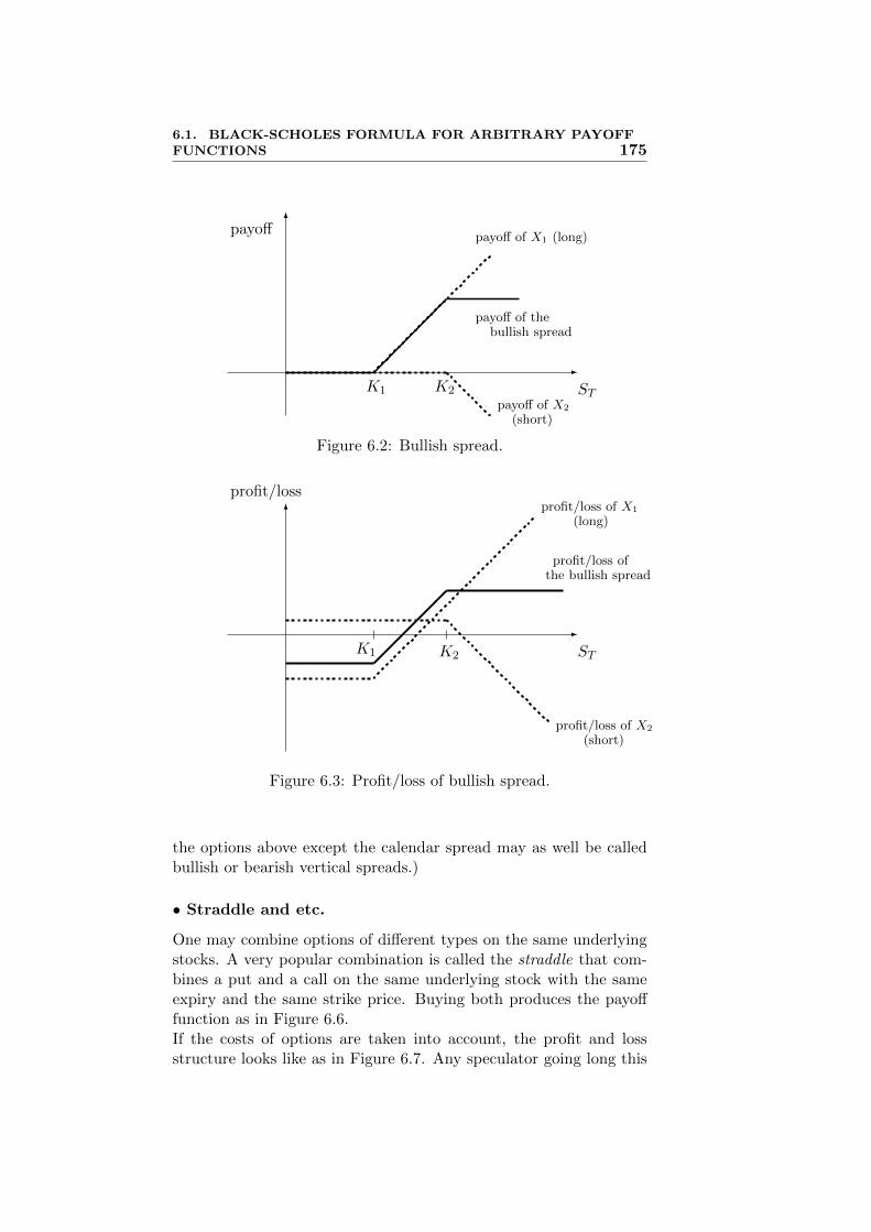
If one combines them by buying X1 and selling X2, the resultingcombination is called a bullish spread whose payoff looks like as inFigure 6.2. If the prices of the constituent options are is taken intoconsideration the payoff function becomes profit/loss and it looks likeas in Figure 6.3.

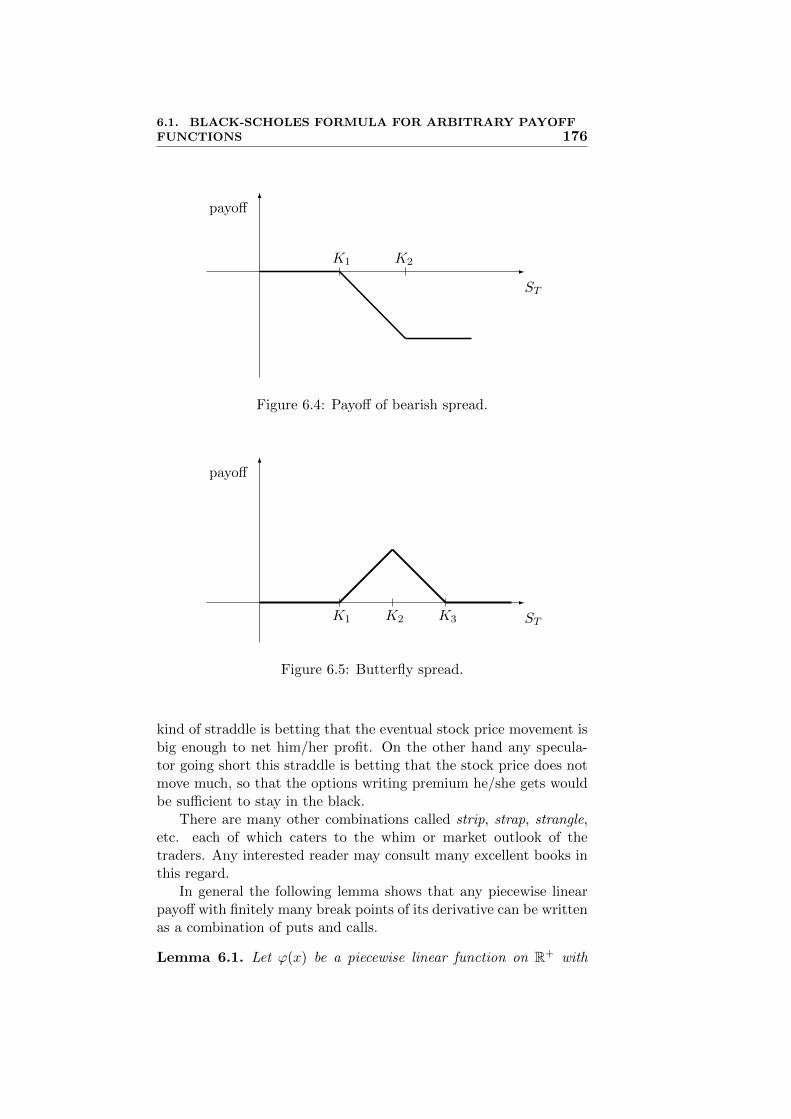
If on the other hand one buys X2 and sell X1, the payoff becomesas in Figure 6.4. This kind of combination is called a bearish spread.

Similarly, one can create a payoff function as in Figure 6.5 bybuying one call option with strike price K1 and another with strikeprice K3 and selling two call options with strike price K2 whereK1 < K2 < K3. This kind combination is called a butterfly spread.

Another kind of spread involves two options of the same kind butwith different expiry. It is generally called a calendar spread, timespread or horizontal spread. (As a way of nomenclature, the “verti-cal” spread means spread involving options with the same expiry. So


payoff

STK1 K2

payoff of X1 (long)

payoff of X2

(short)

payoff of thebullish spread

Figure 6.2: Bullish spread.

profit/loss

STK1 K2

profit/loss of X1

(long)

profit/loss ofthe bullish spread

profit/loss of X2

(short)

Figure 6.3: Profit/loss of bullish spread.

the options above except the calendar spread may as well be calledbullish or bearish vertical spreads.)

• Straddle and etc.

One may combine options of different types on the same underlyingstocks. A very popular combination is called the straddle that com-bines a put and a call on the same underlying stock with the sameexpiry and the same strike price. Buying both produces the payofffunction as in Figure 6.6.If the costs of options are taken into account, the profit and lossstructure looks like as in Figure 6.7. Any speculator going long this


payoff

ST

K1 K2

Figure 6.4: Payoff of bearish spread.

payoff

STK1 K2 K3

Figure 6.5: Butterfly spread.

kind of straddle is betting that the eventual stock price movement isbig enough to net him/her profit. On the other hand any specula-tor going short this straddle is betting that the stock price does notmove much, so that the options writing premium he/she gets wouldbe sufficient to stay in the black.

There are many other combinations called strip, strap, strangle,etc. each of which caters to the whim or market outlook of thetraders. Any interested reader may consult many excellent books inthis regard.

In general the following lemma shows that any piecewise linearpayoff with finitely many break points of its derivative can be writtenas a combination of puts and calls.

Lemma 6.1. Let ϕ(x) be a piecewise linear function on R+ with


payoff

STK

Figure 6.6: Payoff of straddle.

profit/loss

ST

profit/loss ofthe call option

profit/loss ofthe put option

K

Figure 6.7: Profit/loss of straddle.

finitely many discontinuities of ϕ′(x). Then ϕ(x) can be written asa linear combination of finitely many function of the type (x−K)+

or (K − x)+ for suitable finitely many constants K.

We leave the proof of this lemma to the reader. Using it, weimmediately have the following important fact.

Theorem 6.2. Any European contingent claim whose payoff func-tion is a piecewise linear function with finitely many discontinuitiesof its derivative can be constructed as a portfolio of finitely manyEuropean calls and puts, where each constituent option can be heldlong or short according to the sign of coefficient thereof.

6.2. PARAMETER ESTIMATION 178

6.2 Parameter Estimation

In the previous chapter, we learned that the Black-Scholes modelassumes that the stock price St satisfies

logStS0

= µt+ σWt.

(In fact logSt/S0 = (µ− 12σ

2)t+ σWt. But by abuse of notation, weuse µ to denote µ − 1

2σ2.) In this section, we discuss how one can

estimate these parameters µ and σ.Let Sti be the stock price at the end of i-th trading day. Then

logStiSt−1

= µ(ti − ti−1) + σ(Wti −Wti−1)

where ∆t = ti−ti−1 ≈ 1250 . (Here we assume there are approximately

250 trading days per year.) Due to the incremental independence ofthe Brownian motion, we may assume ui = logSti/Sti−1 is a IIDGaussian random variable with mean µ∆t and variance σ2∆t. Bythe standard statistical procedure its mean and variance can be es-timated as:

µ∆t ∼ u =1

n

n∑i=1

ui (6.1)

and1

σ√

∆t ∼ s =

√√√√ 1

n

n∑i=1

u2i − (u)2. (6.2)

We call u the historical daily drift and s the historical daily volatility,respectively. We also call

µ =u

∆t= 250u

and

σ =s√∆t

=s√

1/250≈ 15.81s

the annualized historical draft and volatility, respectively.Let us now see how reliable these estimates are. Table 6.1 shows

various statistical quantities for KOSPI 200 stock price data for everyyear since 2001 till 2010. In there, one can see that |u|2 is two ordersof magnitude smaller than 1

2

∑u2i . Therefore in estimating s, one

may use√

1n

∑u2i instead of

√1n

∑u2i − |ui|2. It has an interesting

1To get an unbiased estimator, one has to use√

1n−1

∑ni=1(ui − u)2. But for

large n they are close enough.

6.2. PARAMETER ESTIMATION 179

u |u|2 1n

∑u2i

√1n

∑u2i

s =√1n

∑u2i − |u|2

σ-estimate(1-year)

µ-estimate(1-year)

2001 0.001163 1.352E-06 4.959E-04 0.022270 0.022239 0.351635 0.290702

2002 -0.000349 1.218E-07 4.482E-04 0.021170 0.021167 0.334683 -0.031020

2003 0.001116 1.245E-06 2.890E-04 0.017001 0.016964 0.268228 0.278905

2004 0.000366 1.340E-07 2.393E-04 0.015469 0.015464 0.244514 0.091511

2005 0.001733 3.003E-06 1.185E-04 0.010887 0.010770 0.169950 0.433205

2006 0.000178 3.157E-08 1.357E-04 0.011650 0.011648 0.184178 0.044419

2007 0.001071 1.147E-06 2.175E-04 0.014750 0.014711 0.232595 0.267739

2008 -0.002016 4.063E-06 6.196E-04 0.024892 0.024810 0.392287 -0.503947

2009 0.001644 2.704E-06 2.641E-04 0.016253 0.016169 0.255656 0.411112

2010 0.000800 6.398E-07 9.988E-05 0.009994 0.009962 0.157516 0.199973

Table 6.1: Historical Volatility and Drift.

statistical consequence. First of all, it enables us to pretend that ui isan IID random variable whose distribution is N(0, σ2∆t). Second, ifso, the independent nature of daily events then means that there areroughly 250 independent samples (one per day) to estimate σ

√∆t

by√

1n

∑u2i .

On the other hand, as |u| is much smaller than√

1n

∑u2i , it is

nearly impossible to extract meaningful “net” changes contributingsolely to u. The 95% confidence interval of u is roughly (−0.00124 +u, 0.00124 + u) when Var(ui) = 0.01, which also indicates that theestimate of u is quite unreliable. So one cannot argue that the inde-pendent nature of daily events cannot be utilized in estimating u orµ. For that reason, one has to use longer period, say the entire year,to get any number for u whose magnitude make sense.

But then as one can see in Table 6.1, µ varies wildly from yearto year, whereas σ is more stable. In other words, the estimation ofσ is statistically more stable than µ. Fortunately, the Black-Schoolsmodel does not depends on µ in any essential way so that the unreli-ability of µ does not pose any serious impedient to using the model.

In practice, no one believes µ or σ stay constant for a long periodof time. Any long term student of market knows that the stock pricemoves like ebbs and flows. There are seasons when the stock pricetends to go up and there are other season when it tanks violently.Accordingly, the volatility for a certain period may be low but itmay flare up in time of crisis. Thus it is advised that one should

6.3. IMPLIED VOLATILITY AND VOLATILITY SMILE 180

take the Black-Schools model as a sort of shorten-term modeling ofthe market.

6.3 Implied Volatility and Volatility Smile

In the previous section, we studied how to estimate the volatilityσ using the historical stock price data. Although this method ofestimating σ is useful in many contexts, it leaves much gap betweenthe model and the actual market price of the options. So many preferto derive σ directly from the market price of a option, hence the nameimplied volatility.

Recall that the Black-Schools formula gives the valuation of acall or put option as a function of the stock price St, the strike priceK, the volatility σ, the interest rate r and the time to expiry T − t.Namely, C is a function2 of such quantities:

C = C(St,K, σ, r, t). (6.3)

Suppose a market price A of a particular option at some instanceof time is given. Treating St,K, r, T − t as known quantities, one canfind σ that satisfies

C(St,K, σ, r, t) = A. (6.4)

To ascertain that such σ exists, one needs to examine the range Acan possibly have.

Recall the Black-Schools formula for the call option

Ct = StN(d1)− e−r(T−t)KN(d2).

where

d1 =log(St/Ke

−r(T−t)) + 12σ

2(T − t)σ√T − t

d2 =log(St/Ke

−r(T−t))− 12σ

2(T − t)σ√T − t

= d1 − σ√T − t.

Using this formula, one can check how Ct changes as one varies σwhile holding all other parameters fixed. Let us first check the how Ctbehaves as σ → 0. It is trivial to see that if St < Ke−r(T−t), d1 andd2 → −∞, hence N(d1) and N(d2)→ 0. Therefore Ct converges to 0.If, on the other hand, St > Ke−r(T−t), d1 and d2 → +∞, henceN(d1)and N(d2) → 1. Therefore Ct converges to St − Ke−r(T−t). The

2In fact, C is a function of the form C(St,K, σ, r, T − t). But since T is fixed,we express C in the form (6.3).


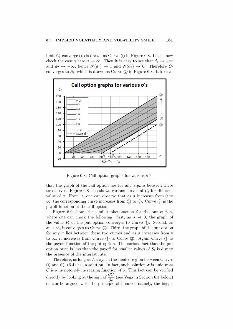
limit Ct converges to is drawn as Curve 1© in Figure 6.8. Let us nowcheck the case where σ →∞. Then it is easy to see that d1 → +∞and d2 → −∞, hence N(d1) → 1 and N(d2) → 0. Therefore Ctconverges to St, which is drawn as Curve 2© in Figure 6.8. It is clear

Figure 6.8: Call option graphs for various σ’s.

that the graph of the call option lies for any sigma between theretwo curves. Figure 6.8 also shows various curves of Ct for differentvalue of σ. From it, one can observe that as σ increases from 0 to∞, the corresponding curve increases from 1© to 2©. Curve 3© is thepayoff function of the call option.

Figure 6.9 shows the similar phenomenon for the put option,where one can check the following: first, as σ → 0, the graph ofthe value Pt of the put option converges to Curve 1©. Second, asσ →∞, it converges to Curve 2©. Third, the graph of the put optionfor any σ lies between these two curves and as σ increases from 0to ∞, it increases from Curve 1© to Curve 2©. Again Curve 3© isthe payoff function of the put option. The curious fact that the putoption price is less than the payoff for smaller values of St is due tothe presence of the interest rate.

Therefore, as long as A stays in the shaded region between Curves1© and 2©, (6.4) has a solution. In fact, such solution σ is unique asC is a monotonely increasing function of σ. This fact can be verified

directly by looking at the sign of∂C

∂σ(see Vega in Section 6.4 below)

or can be argued with the principle of finance: namely, the bigger


Figure 6.9: Put option graphs for various σ’s.

the volatility, the higher the chance for profit for the holder of theoption; hence, the higher the option value.

The value of σ calculated this way is called the impled volatility,meaning that the volatility is inferred from the market price data ofthe option via the Black-Schools formula.

Figure 6.10: Implied volatility graph for KOSPI 200 call options.

6.4. SENSITIVITY ANALYSIS: GREEKS 183

Figure 6.10 shows the impled volatility against the various strikeprices. According to the assumption of the Black-Schools model, σis supposed to be a constant. Therefore the implied volatilities mustbe constant for different Ks. But as one can see in Figure 6.10, itis not the case. Such phenomenon is usually called the (volatility)smile. It shows that the assumption of the Black-Schools model doesnot match what is really going on in the options market.

This volatility smile has many practical implications for traders.To make the Black-Schools model to conform to this phenomenon,one sometimes uses a model for which σ is a stochastic process.(There is a debate as for the utility of such model.) A particulartype of such stochastic volatility model is to set σ as a deterministicfunction of t and St, i.e.,

σ = σ(t, St).

Luckily even if σ is of this form, all the derivations in Chapter 5leading to the Black-Schools PDE are valid. So we have followingboundary value problem.

∂V

∂t+ rS

∂V

∂S+

1

2σ(t, S)2S2∂

2V

∂S2− rV = 0

V (T, S) = ϕ(S).

This PDE is still linear. But unless σ(t, St) is of particular form,its solution can only be computed by numerical methods.

There are more general form of stochastic volatility for whosesolution one uses a more sophisticated Monte-Carlo method. But wewill not go into this in this lecture.

6.4 Sensitivity Analysis: Greeks

It is always a good practice to understand how a formula (for thatmatter, any recipe or even a theory) changes as the parameter varies.Examining such phenomenon is generally called a sensitive analysis.

In this section, we examine various rates of change of the Black-Schools formula with respect to the change of each important pa-rameter. (In this section, when we draw a specific graph, the optionvalues are computed assuming K = 100, σ = 25% and r = 5%.)

• Delta

Delta is the rate of change of the option value with respect to thestock price and is denote as:

∆ =∂V

∂S


Delta of a call optionLet Ct be a call option vale at time t. Recall that the Black-Schoolsformula for a call option is

Ct = StN(d1)− e−r(T−t)KN(d2). (6.5)

Differentiating both sides with respect to St, we have

∆ =∂Ct∂St

= N(d1) + StN′(d1)

∂d1

∂St− e−r(T−t)KN ′(d2)

∂d2

∂St.

Since d2 = d1 − σ√T − t and N ′(x) is the normal density function,

i.e., (2π)−12 exp(−x2/2), we get

∆ = N(d1) +∂d1

∂St

[StN

′(d1)− e−r(T−t)KN ′(d1 − σ√T − t)

]= N(d1) +

∂d1

∂St

[StN

′(d1)− e−r(T−t)K exp

(d1σ√T − t− 1

2σ2(T − t)

)N ′(d1)

]= N(d1) +

∂d1

∂St

[StN

′(d1)− e−r(T−t)K exp(

log(St/K) + r(T − t))N ′(d1)

]= N(d1).

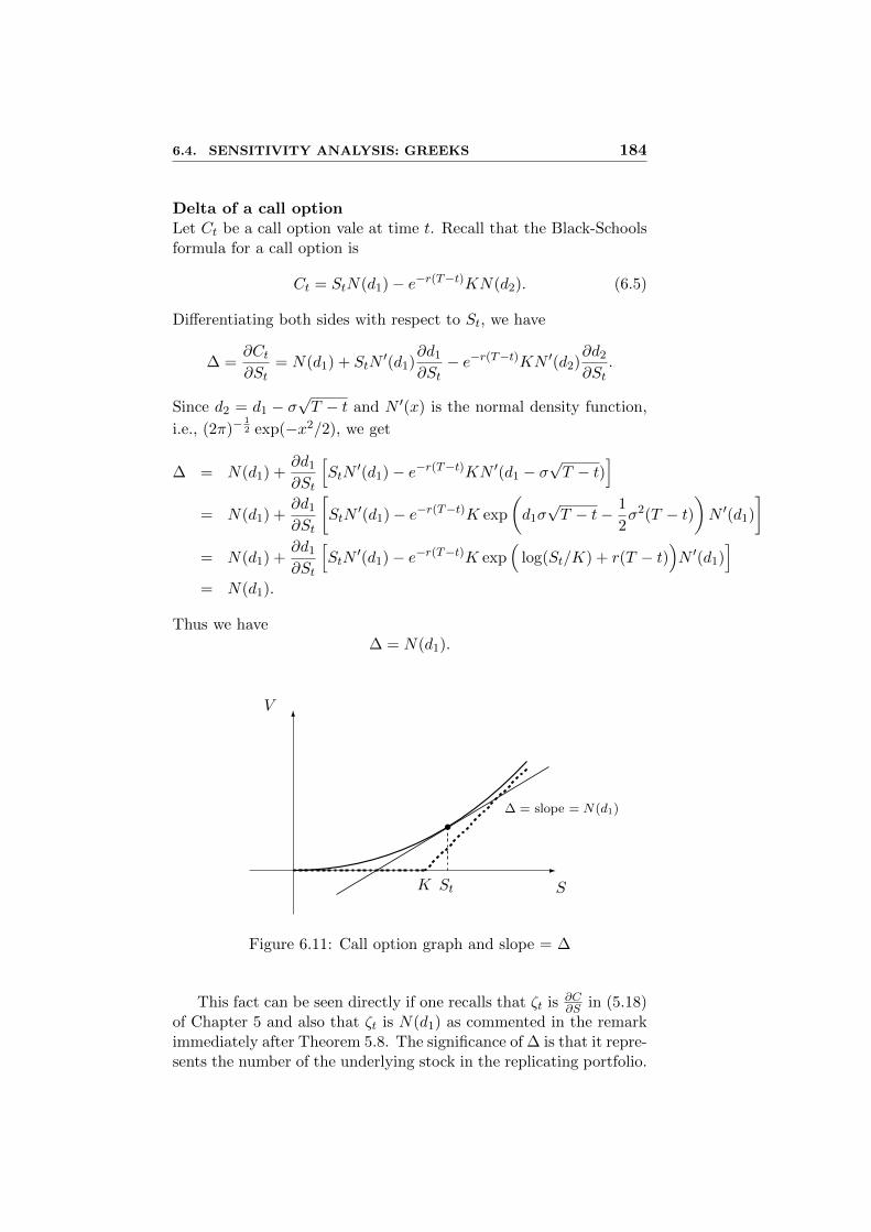
Thus we have∆ = N(d1).

V

SK St

∆ = slope = N(d1)

Figure 6.11: Call option graph and slope = ∆

This fact can be seen directly if one recalls that ζt is ∂C∂S in (5.18)

of Chapter 5 and also that ζt is N(d1) as commented in the remarkimmediately after Theorem 5.8. The significance of ∆ is that it repre-sents the number of the underlying stock in the replicating portfolio.


Figure 6.12: Delta graph of a call option.

But the same token, e−rTKN(d2) is the amount of bank borrowingfor the replicating portfolio. (See Theorem 5.8 and the commentthereafter.)

Figure 6.11 shows the graph of the value of a call option togetherwith its Delta for given St. It is very important to note that the Deltais the slope of the graph at St. It is also important to note that theDelta increases as St increases, which means that as St increases thereplicating portfolio must increase the number of stocks in it.

Figure 6.12 also shows the Delta as a function of St. One can seethat the Delta changes most rapidly near the strike price.

Delta of a put optionLet Pt be a put option value at time t and ∆C the Delta of a calloption. From the put-call parity, we have

Pt = Ct + e−r(T−t)K − St

Differentiating both sides with respect to St, we have

∂Pt∂St

= ∆C − 1 = N(d1)− 1 = −N(−d1).

Thus the Delta of a put option is

∆ = −N(−d1).

This fact can also be seen directly from the Black-Schools formulaas in done for the call option.

Figure 6.13 shows the graph of a put option and its Delta as someSt. The negative slope indicates that the replicating portfolio musthave a short position of the underlying stock.


V

S

K St ∆ = slope = −N(−d1)

Figure 6.13: Put option graph and slope = ∆

Figure 6.14: Delta graph of a put option.

• Gamma

Gamma is the rate of change of Delta with respect to the stock priceand is denoted by

Γ =∂∆

∂S=∂2V

∂S2.

Gamma of a call or put optionLet C be a call option’s value. Then

Γ =∂∆

∂S=

∂

∂StN(d1) = N ′(d1)

∂d1

∂St=

N ′(d1)

Stσ√T − t

.


From the put-call parity, we can easily check that the Gamma of acall and the Gamma of a put have the same value. So, we get

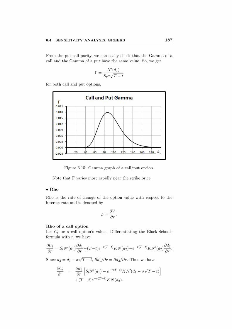
Γ =N ′(d1)

Stσ√T − t

for both call and put options.

Figure 6.15: Gamma graph of a call/put option.

Note that Γ varies most rapidly near the strike price.

• Rho

Rho is the rate of change of the option value with respect to theinterest rate and is denoted by

ρ =∂V

∂r.

Rho of a call optionLet Ct be a call option’s value. Differentiating the Black-Schoolsformula with r, we have

∂Ct∂r

= StN′(d1)

∂d1

∂r+(T−t)e−r(T−t)KN(d2)−e−r(T−t)KN ′(d2)

∂d2

∂r.

Since d2 = d1 − σ√T − t, ∂d1/∂r = ∂d2/∂r. Thus we have

∂Ct∂r

=∂d1

∂r

[StN

′(d1)− e−r(T−t)KN ′(d1 − σ√T − t)

]+(T − t)e−r(T−t)KN(d2).


As in the calculation of the Delta, we already know that

StN′(d1)− e−r(T−t)KN ′(d1 − σ

√T − t) = 0.

Thus we haveρ = (T − t)e−r(T−t)KN(d2).

Figure 6.16: Rho graph of a call option.

Figure 6.16 shows the change of ρ with respect to S. In particular,note that since ρ is always positive, the call option’s value increasesas the interest rate increases.

Rho of a put optionCombining the put-call parity and the Rho value of a call option, wecan easily get the Rho of a put option.

ρ = −K(T − t)e−r(T−t)N(−d2).

Since ρ is always negative, the option’s value decreases as theinterest rate increases.

• Theta

Θ is the rate of change of the option value with respect to the timeand is defined by

Θ =∂V

∂t.


Figure 6.17: Rho graph of a put option.

Theta of a call optionSince ∂V/∂t = −∂V/∂(T − t), we use τ = (T − t) instead of t in thefollowing calculation. Differentiating a call option value Ct that isgiven from the Black-Schools formula, we have

∂Ct∂τ

= StN′(d1)

∂d1

∂τ+ re−rτKN(d2)− e−rτKN ′(d2)

∂d2

∂τ.

Since ∂d1/∂τ = ∂d2/∂τ + σ/(2√τ) and

StN′(d1)− e−rτKN ′(d2) = 0,

replacing ∂d1/∂τ with ∂d2/∂τ + 1/(2√τ), we have

∂Ct∂τ

=StσN

′(d1)

2√τ

+ rKe−rτN(d2).

Thus we have

Θ = −StσN′(d1)

2√T − t

− rKe−r(T−t)N(d2)

= −Stσ exp

(−d2

1/2)

2√

2π(T − t)− rKe−r(T−t)N(d2).

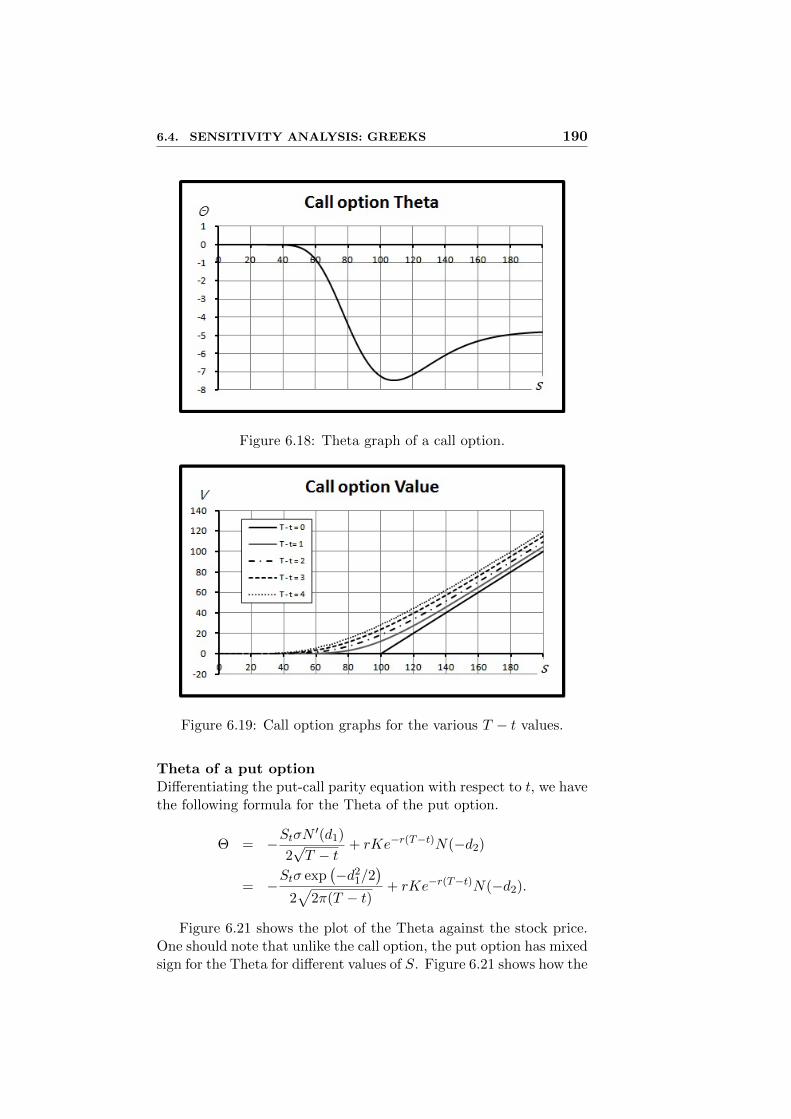
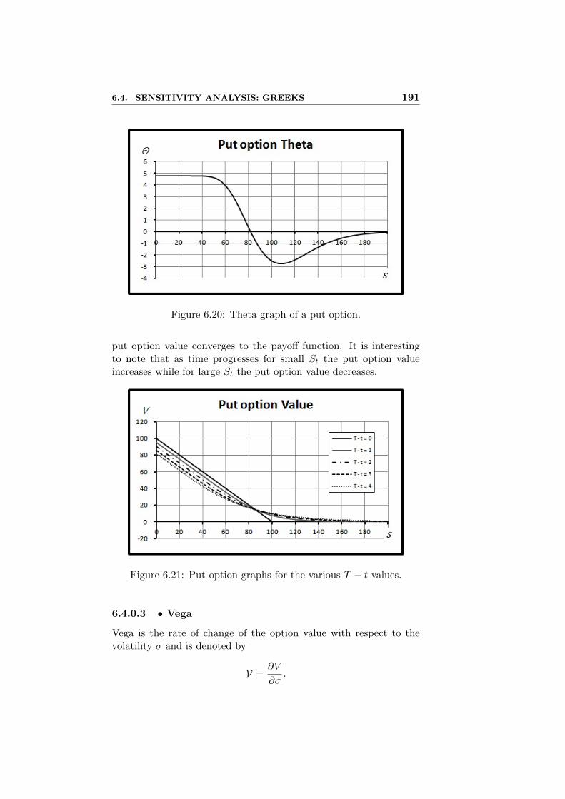
Since Θ is always negative, the value of the call option decreasesas time progresses. Figure 6.19 shows the pattern of the call option’svalue converging monotonically to the payoff as time passes.


Figure 6.18: Theta graph of a call option.

Figure 6.19: Call option graphs for the various T − t values.

Theta of a put optionDifferentiating the put-call parity equation with respect to t, we havethe following formula for the Theta of the put option.

Θ = −StσN′(d1)

2√T − t

+ rKe−r(T−t)N(−d2)

= −Stσ exp

(−d2

1/2)

2√

2π(T − t)+ rKe−r(T−t)N(−d2).

Figure 6.21 shows the plot of the Theta against the stock price.One should note that unlike the call option, the put option has mixedsign for the Theta for different values of S. Figure 6.21 shows how the


Figure 6.20: Theta graph of a put option.

put option value converges to the payoff function. It is interestingto note that as time progresses for small St the put option valueincreases while for large St the put option value decreases.

Figure 6.21: Put option graphs for the various T − t values.

6.4.0.3 • Vega

Vega is the rate of change of the option value with respect to thevolatility σ and is denoted by

V =∂V

∂σ.


Vega of a call or put optionSince ∂d1

∂σ = ∂d2∂σ +

√T − t, we have

V =∂Ct∂σ

= StN′(d1)

∂d1

∂σ− e−r(T−t)KN ′(d2)

∂d2

∂σ

=∂d2

∂σ

[StN

′(d1)− e−rτKN ′(d2)]

+ St√T − tN ′(d1)

= St√T − tN ′(d1).

Differentiating the put-call parity equation with respect to σ one cansee that the Vega of a call and the Vega of a put are the same. Thusfor both call and put options, we have

V = St√T − t N ′(d1)

= St√T − t

exp(−d2

1/2)

√2π

.

Note that the Vega is always positive, which means that the val-ues of the call and put options increases as the volatility increases.The reader is advised to go back Section 6.3 concerning such changes.

Figure 6.22: Vega graph of a call option.

• Greeks of general contingent claim

So far in this section, we have confined ourselves to the Greeks ofthe call or put options. But the concept of Greeks applies to anycontingent claim with arbitrary payoff functions.

To see how it goes, let X be a European option with expiry Twith payoff function ϕ(ST ). Then by the verbatim application of

6.5. DELTA AND GAMMA HEDGING 193

the arguments in Section 5.5 the value Vt of X at time t is given byVt = V (t, S), where V (t, S) is the solution of the following bound-ary(terminal) value problem:

∂V

∂t+ rS

∂V

∂S+

1

2σ2S2∂

2V

∂s2− rV = 0

V (T, S) = ϕ(S).

(6.6)

Then as before the Greeks of X are defined as follows;

- Delta: ∆ = ∂V∂S (t, St)

- Gamma: Γ = ∂∆∂S (t, St) = ∂2V

∂S2 (t, St)

- Rho: ρ = ∂V∂r (t, St)

- Theta: Θ = ∂V∂t (t, St)

- Vega: V = ∂V∂σ (t, St).

In particular, if ϕ(S) is a continuous piecewise linear functionwith finite number of discontinuities of its derivative, Theorem 6.2implies that X can be constructed as a portfolio (linear combination)of finite number of calls and puts. Any Greek of such X is the samelinear combination of the corresponding Greeks of constituent callsor puts. In particular, the Greeks of the spreads, the straddles andthe likes can be computed this way.

6.5 Delta and Gamma Hedging

6.5.1 Continuous Delta Hedging

Let X be a European option with payoff function ϕ(ST ), where Tis the expiry. Then its value Vt at time t is given by Vt = V (t, S),where V (t, S) is the solution of (6.6).

In Section 5.5, we showed that the replicating portfolio (ξt, ζt) isgiven in such a way that

ζt = ∆ =∂V

∂S(t, St),

ξt = e−rt[Vt −∆St].

(See (5.26) of Chapter 5 for further details.)As time progresses, the delta

∆ = ∆t =∂V

∂St


changes continuously. Thus the replicating portfolio has to be read-justed accordingly. In the parlance of finance, this continuous read-justment is called the continuous hedging or continuous delta hedging.However, this “continuous” hedging is only a theoretical construct;in practice there is no way to do anything continuously (i.e., infinitelyoften). At best one can do is to trade (hedge) frequently. This gapbetween theory and practice may be negligible in many cases butwhen the stock price moves rapidly it could be a cause for seriousconsequences.

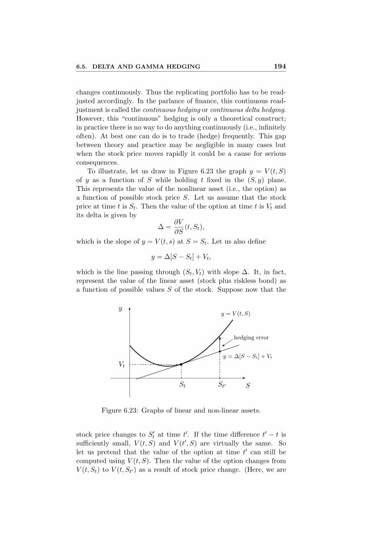
To illustrate, let us draw in Figure 6.23 the graph y = V (t, S)of y as a function of S while holding t fixed in the (S, y) plane.This represents the value of the nonlinear asset (i.e., the option) asa function of possible stock price S. Let us assume that the stockprice at time t is St. Then the value of the option at time t is Vt andits delta is given by

∆ =∂V

∂S(t, St),

which is the slope of y = V (t, s) at S = St. Let us also define

y = ∆[S − St] + Vt,

which is the line passing through (St, Vt) with slope ∆. It, in fact,represent the value of the linear asset (stock plus riskless bond) asa function of possible values S of the stock. Suppose now that the

y

SSt St′

Vt

y = V (t, S)

y = ∆[S − St] + Vt

hedging error

Figure 6.23: Graphs of linear and non-linear assets.

stock price changes to S′t at time t′. If the time difference t′ − t issufficiently small, V (t, S) and V (t′, S) are virtually the same. Solet us pretend that the value of the option at time t′ can still becomputed using V (t, S). Then the value of the option changes fromV (t, St) to V (t, St′) as a result of stock price change. (Here, we are


assuming there is no trade throughout this change.) Similarly, thevalue of the linear asset (i.e., the replicating portfolio) changes fromVt to ∆[St′−St]+Vt. Then the values of the option and the replicatingportfolio do not coincide, which is usually called the hedging error.It is depicted in Figure 6.23. Seen from the viewpoint of the option’swriter (seller), this hedging error represents the loss. Figure 6.24shows the hedging error as a function of S (= St′).

y

SSt

Figure 6.24: Hedging error (loss) of the option’s writer.

Figure 6.25 shows the effect of the change of the option’s valuedue to the change in time. Depending on the shape of the graph ofy = V (t, S), this time value may help or hurt the option’s writer.

y

SSt St′

y = V (t, S)

y = V (t′, S)

actual hedging error

Figure 6.25: Actual hedging error with the time value taken in.

In any case, if the stock price moves rapidly in short time, thechange of the option’s value due to time value is relatively small,and the dominant factor is the kind of hedging error described in


Figure 6.24. To minimize such hedging error, one is forced to tradefrequently, and more importantly, the option’s writer should have de-manded enough premium over the Black-Schools price to compensatefor such contingencies.

6.5.2 Gamma Hedging

The shortcomings of the delta hedging are by now clear. Namely, it isvulnerable to big changes in the stock price in a short time. In orderto rectify it, the traders frequently employ the so-called delta-gammahedging, or in short the gamma hedging. The idea is rather simple.Instead of using the linear assets (stocks and riskless bonds) thathave no gamma, the hedging is done by utilizing the plain vanilla(put and call) options that are abundantly available.

Suppose V = V (t, S) is the value of the option to be hedged.Let ∆V and ΓV be its delta and gamma, respectively. Construct aportfolio consisting of two other vanilla options: Option 1 and Option2. Let the delta and gamma of Option 1 be denoted by ∆1 and Γ1.Similarly, let ∆2 and Γ2 be the delta and gamma of Option 2. Letx be the number of units of Option 1 in the portfolio and y thatof Option 2. Then the delta of such portfolio is ∆P = x∆1 + y∆2

and the gamma of the portfolio is ΓP = xΓ1 + yΓ2. We can find theappropriate values of x and y such that ∆P = x∆1 + y∆2 = ∆V

ΓP = xΓ1 + yΓ2 = ΓV .(6.7)

This is a system of linear equation for x and y that can be solvedquite easily. The effect of having this portfolio consisting of twooptions is that its value at St matches that of V = V (t, S) up tosecond order at St, which is depicted in Figure 6.26.

By adding more options to the portfolio one can match moreGreeks. For instance, let us add another vanilla option, called Option3. Let ∆3, Γ3 be its delta and gamma, respectively. Furthermore,let Λ1, Λ2 and Λ3 be the vegas of Option 1, 2 and 3. Then one canfind x, y and z such that

x∆1 + y∆2 + z∆3 = ∆V

xΓ1 + yΓ2 + zΓ3 = ΓV

xΛ1 + yΛ2 + zΛ3 = ΛV

(6.8)

where ΛV is the vega of option V in question.It is obvious that by adding more and more options this way, one

can match all the Greeks.

6.6. PORTFOLIO INSURANCE 197

y

SSt

y = V (t, S)

value of the portfolioconsisting of two options

Figure 6.26: Portfolio’s value matches V up to second order.

This method of utilizing several non-linear assets (i.e., vanilla calland put options) to match various or all Greeks works even when Vis not a single option but itself a portfolio of stocks, options and(riskless) bonds.

However the trouble with this method is that the resulting sys-tem of equations may be numerically ill-conditioned, which mayyield widely varying, and sometime unrealistic, numerical values forx, y, z, etc. as the parameter changes slightly. So some sort of sta-bilization scheme must be employed. Furthermore, there are manychoices for Option 1, 2, 3, etc. to match the delta, gamma, vega, etc.of V . In fact, which options to utilize is a critical question for whichmany other aspects must be considered. For instance, the liquidityand the price should be just as important factors.

6.6 Portfolio Insurance

Portfolio insurance is a method/technique developed by Leland andRubinstein that purports to “insure” a portfolio, if properly con-structed and managed according to their recipe, against the down-side risk while keeping open the upside potential due to the rise ofthe stock price. It was conceived in late 1970s and was actively mar-keted in the 1980s until its shortcomings were revealed in the crashof 1987.

The idea of the portfolio insurance is rather simple. Suppose Stis a stock price or rather a price of an index like S&P 500 that ishugely liquid. Its put-call parity says that

St + Pt = Ct +Ke−r(T−t)


where Pt and Ct are the prices of the put and the call with expiryT and strike price K, respectively. Using the Black-Scholes formula,(5.43) of Chapter 5, we have

St + Pt = N(d1)St +Ke−r(T−t)(1−N(d2)). (6.9)

This formula can be interpreted as saying that the portfolio consist-ing of one stock and a put option is equivalent to holding N(d1)shares of stock and 1−N(d2) units of riskless bond whose face value(i.e., the amount to be paid at the maturity T ) is K, or by the sametoken, K(1−N(d2)) units of riskless bonds each of which pays 1 atT .

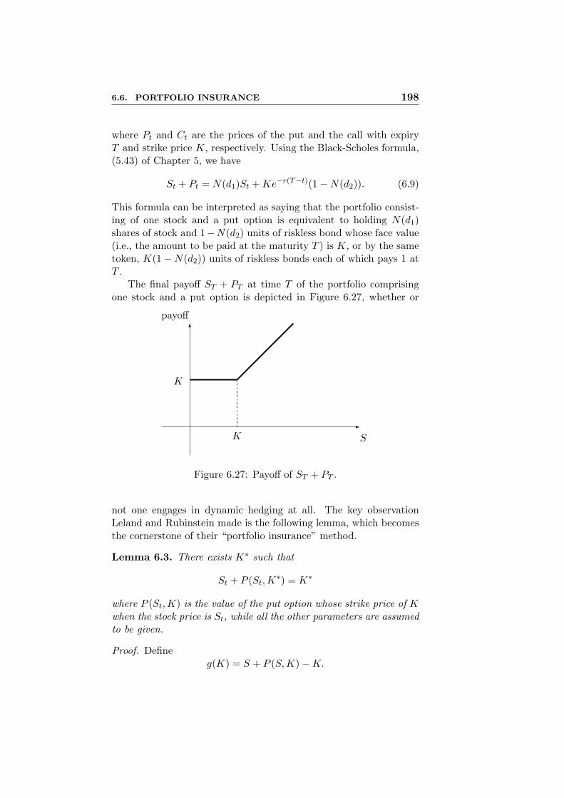
The final payoff ST + PT at time T of the portfolio comprisingone stock and a put option is depicted in Figure 6.27, whether or

payoff

SK

K

Figure 6.27: Payoff of ST + PT .

not one engages in dynamic hedging at all. The key observationLeland and Rubinstein made is the following lemma, which becomesthe cornerstone of their “portfolio insurance” method.

Lemma 6.3. There exists K∗ such that

St + P (St,K∗) = K∗

where P (St,K) is the value of the put option whose strike price of Kwhen the stock price is St, while all the other parameters are assumedto be given.

Proof. Defineg(K) = S + P (S,K)−K.


Then g(0) = S, since P (S, 0) = 0. On the other hand, as K → ∞,we can check that d1 → −∞ and d2 → −∞. Therefore by (6.9)

g(K) = SN(d1) +Ke−r(T−t)(1−N(d2))−K→ −K(1− e−r(T−t)) < 0.

Thus by the continuity of g(K), there must be K∗ such that g(K∗) =0.

This lemma is remarkable in the sense that it opens up a pos-sibility, albeit theoretical, of minting money. Namely, if one startswith a sum of K∗ dollars and use it to buy one share of stock and aput option with the strike price K∗, the payoff structure as in Fig-ure 6.27 guarantees that at time T one cannot lose money but has apossibility of making money in case ST > K∗. (Of course, we haveignored important details like transaction costs, etc.)

Leland and Rubinstein went ahead and tried to exploit this idea.The trouble is that such put option with strike price K∗ was notalways available in the market place, and even if it was, it may nothave been available in sufficient quantity. They therefore decided tosynthetically create the portfolio by utilizing (6.9). The left had sideof (6.9) is the “magic portfolio” that can “mint” money, which isequal to the right hand side of (6.9). As we said in the commentimmediately following (6.9), the right hand side says that as long asone dynamically maintains the portfolio consisting of N(d1) sharesof stocks and 1 − N(d2) units of riskless bond with face value K∗,the final payoff will be ST +P (ST ,K

∗) which is always greater thanor equal to the initial investment K∗.

However, this portfolio insurance technique did not live up to itspromise in time of crisis. In fact, it simply melted down shortly be-fore, during and after the Black Monday of 1987 (October 19, 1987).According to the Brady Commission Report, during the three-dayperiod of October 14 to October 16, 1987, there was a $12 billionworth of portfolio insurance outstanding and only $4 billion worthwas properly executed according to the plan of portfolio insurance,and at the peak of crash, on Monday, October 19th, 10% of the salesvolume of NYSE and 21% of the index futures sales were due toportfolio insurance. What happened was that the sell orders trig-gered by the dynamic hedging method were left unexcuted while thestock price was dropping precipitously. In short, the dynamic hedg-ing scheme envisioned by the designers of portfolio insurance failedto function properly, which resulted in big loss.

There are many reasons for this failure. To list a few:

• As the stock market declines, the delta hedging method em-ployed by the portfolio insurance triggers even more sell orders

6.7. DIVIDEND MODELS 200

due to the convex nature of its value function. This helps addgreater downward pressure on the stock price, hence creatinghuge market instability.

• When there are overwhelmingly more sell orders than buy or-ders, the sell orders not be properly executed, Thus therebydefeating the purpose of the portfolio insurance. (This is inmarked contrast with the usual insurance where the events oc-cur sporadically with very low correlation.)

6.7 Dividend models

Dividend is a stream of cash paid to the holder of a stock. This cashpayment occurs at discrete times that are fixed a priori beforehandor they can be ramdom. The amount of dividend at each dividendpayment time can be predetermined or it can vary randomly. In thissection, we study two models of dividend. The first is the one ofdeterministic discrete dividend model and the second is the so-calledconstant dividend model.

6.7.1 Known discrete dividend model

Let t = 0 be the present and let Ti be the time of dividend paymentwith dividend amount Ki and let T be the time at which our optionexpires.

0 T1 T2 Ti T· · ·· · ·

K1 K2 Ki · · ·· · ·

Suppose the interest rate r is a constant. Then the value It at timet of all the dividend paid after t until T is

It =∑i

Kie−r(Ti−t)1(t,T ](Ti).

Similarly the value It at time T of all the dividend paid after t untilT is

It =∑i

Kier(T−Ti)1(t,T ](Ti).

When dividend is paid the stock price usually drops by a fixedamount, which is called an ex-dividend drop. Thus it is not a goodidea to deal with the stock price process directly. Instead, after


Heath and Jarrow, we primarily deal with the so-called capital gainsprocess Gt, which is assumed to satisfy

dGt = Gt(µdt+ σdWt) (6.10)

Let Dt be the value at t of the totality of the dividends paid afterthe present (t = 0) until time t. Then obviously

Dt =∑i

Kier(t−Ti)1(0,t](Ti).

Note in particular thatDT = I0.

The net capital gain from time 0 to t is Gt − G0. It is certainlycomposed of that coming from the appreciation of stock price(St−S0)and the value at t of the totality of dividends paid after 0 until t.Therefore

Gt −G0 = St − S0 +Dt.

Taking differential, we have

dGt = dSt + dDt (6.11)

We set G0 = S0, if there is no dividend payment at time t = 0; and ifthere is a dividend payment at t = 0, we set S0 to be the ex-dividendprice. Hence in either case we have:

G0 = S0,

Gt = St +Dt.

The trading strategy is as usual composed of ζt shares of St andξt units of bank account. Then the value process of the portfolio is

Vt = ζtSt + ξtBt.

We now assume that the dividend is reinvested in the same stockimmediately after the dividend is paid. With this in mind, let usrecall the true meaning of “self-financing” condition. A portfolio isself financing if the change of its value is entirely due to the internalmarket dynamics with no money coming in from or going out tothe outside world. Cast in this viewpoint, this portfolio must beself-financing if the change of the portfolio’s, value is due to first,the change in stock price; second, the increase in bank account; andthird, the dividend. Therefore it is eminently reasonable to define(ζt, ξt) is self-financing if and only if

dVt = ζtdSt + ξtdBt + ζtdDt.


This and (6.11) then imply that

dVt = ζtdGt + ξtdBt.

This together with (6.10) means that we can work with Gt insteadof St in deriving the options value formula. Note that

GT = ST +DT = ST + I0.

Let X = (ST −K)+ be a European call option. Rewritten in termsof Gt, we have

X = (GT − (K + I0))+, (6.12)

whereGt satisfies the usual geometric Brownian motion (6.10). There-fore one can apply the usual machinery of deriving the Black-Scholesformula with Gt replacing St (In here, one has to check that theportfolio is self-financing and it replicates X, etc. But they are alleasy exercises and hence are left to the reader.)

The key point in (6.12) is that the exercise price K is replacedwith K + I0. Therefore we have the call option value formula

C0 = G0N(d1)− e−rT (K + I0)N(d2),

where

d1 =log(S0/(K + I0)) + (r + 1

2σ2)T

σ√T

,

d2 =log(S0/(K + I0)) + (r − 1

2σ2)T

σ√T

.

Similarly, by translating time, we have the following:

Theorem 6.4. Suppose St satisfies the conditions described abovewith known discrete dividend payments. The value Ct at time t ofthe call option with strike price K at expiry T is given by

Ct = StN(d1)− e−r(T−t)(K + It)N(d2),

where

d1 =log(St/(K + It)) + (r + 1

2σ2)(T − t)

σ√T − t

,

d2 =log(St/(K + It)) + (r − 1

2σ2)(T − t)

σ√T − t

.

Here, St is the ex-dividend stock price at time t and It is the valueat t of the dividends paid after t until T .


6.7.2 Constant dividend yield model

Another simplifying model on dividend is that of constant dividendyield. The gist of this model is that unlike the one in the previoussubsection, one assumes that the dividend is paid out at a constantrate like the continuously compounding interest rate model. Thuswe assume that if the stock price at t is St the dividend paid outduring the short time interval [t, t+ dt] is proportional to St, i.e.

dDt = δStdt, (6.13)

where Dt is the sum(∫

) of dividends paid out from time 0 to t andδ is a positive constant called the dividend payout ratio. We fur-ther assume that the dividend is immediately reinvested in the samestock. Thus the dividend dDt = δStdt paid out during [t, t+dt] buysδdt shares of stocks. Therefore the holder of the stock actually hasincreasing number of the stock. he/she holds. Let Ut be the numberof the stock due to this reinvestment. Since (6.13) is for a singleshare, the dividend received by the holder of Ut shares is

dDt = δStUtdt,

which buysdUt = δUtdt (6.14)

shares of socks. Assuming U0 = 1, (6.14) yields

Ut = eδt.

Assume now that St satisfies the usual geometric Brownian mo-tion

dSt = St(µdt+ σdWt),

which gives

St = S0 exp

((µ− 1

2σ2)t+ σWt

).

Therefore the value St of Ut = eδt shares of such stock is

St = Steδt

= S0 exp

((µ− 1

2σ2 + δ)t+ σWt

).

Rewriting this, we can easily see that

dSt = St((µ+ δ)t+ σWt). (6.15)


Let (ζt, ξt) be a portfolio of ζt shares of St and ξt units of bankaccount. Then its value Vt is given by

Vt = ζtSt + ξtBt.

As we did in the previous subsection, the self-financing portfolio’svalue change comes from the three source: the change in stock price,the change in bank account and the dividend. Therefore the self-financing condition can be phrased as:

dVt = ζtdSt + ξtdBt + ζtδStdt.

is the self-financing condition. Thus for the self-financing portfolio,

dVt = ζtSt[(µ+ δ)dt+ σdWt] + ξtdBt

= e−δtζtSt[(µ+ δ)dt+ σdWt] + ξtdBt

= e−δtζtdSt + ξtdBt,

where in the second equality St = Steδt is used and in the third

equality (6.15) is used. Define ζt = e−δtSt. Then we have

dVt = ζtdSt + ξtdBt.

From this, we can conclude that

Lemma 6.5. The portfolio (ζt, ξt) consisting of ζt shares of St andξt units of Bt, assuming constant dividend yield, is self-financing ifand only if the portfolio (ζt, ξt) consisting of ζt shares of(hypothetical)stock St and ξt units of Bt is self-financing in the usual sense, i.e.,

dVt = ζtdSt + ξtdBt.

With this lemma the usual machinery of the Black-Scholes modeltakes over to give us the options formula. In particular, let X =(ST − K)+ be a European call option with strike price K at theexpiry T . Rewriting it, we have

X = e−δT (ST −KeδT )+.

Thus using the usual Black-Scholes formula, the value Ct of the calloption at time t is seen to be

Ct = e−δT [StN(d1)− e−r(T−t)KeδTN(d2)], (6.16)

where

d1 =log(St/Ke

δT ) + (r + 12σ

2)(T − t)σ√T − t

,

d2 =log(St/Ke

δT ) + (r − 12σ

2)(T − t)σ√T − t

.


Using St = eδtSt, one can rewrite (6.16) to get the following

Ct = e−δ(T−t)[StN(d1)− e−(r−δ)(T−t)KN(d2)],

where

d1 =log(St/K) + (r − δ + 1

2σ2)(T − t)

σ√T − t

,

d2 =log(St/K) + (r − δ − 1

2σ2)(T − t)

σ√T − t

.

By the put-call parity, the put option price is also easily seen as

Pt = e−δ(T−t)[−StN(−d1) + e−(r−δ)(T−t)KN(−d2)].

EXERCISES 206

Exercises

6.1.

Answer ”yes” or ”no” to the following assertion related to the greeksof the Black-Scholes formula. Briefly explain why.

(a) The higher the volatility, the higher the value of a put option.

(b) The higher the stock price, the more shares of stock the hedgingportfolio of a call option must have

(c) As the stock price decreases, the seller of a put option mustsell more shares short in the hedging portfolio

(d) As the interest rate increases, the value of the put option in-creases.

(e) All things being equal, the value of a put option increases astime passes if it is deeply in in-the-money territory.

6.2.

(a) Write down the Black-Scholes formula for the call option in thecase of constant dividend yield rate δ.

(b) What will Ct converge to as σ →∞?

(c) What will Ct converge to as σ → 0?

Documents

Rami cations of the Black-Scholes Model · 2012-11-07 · 6.1. BLACK-SCHOLES FORMULA FOR ARBITRARY PAYOFF FUNCTIONS 174 As a practical matter, one usually relies on numerical method