Ramanujan graphs in cryptography

Anamaria Costache1, Brooke Feigon2, Kristin Lauter3, Maike Massierer4, and AnnaPuskas5

1Department of Computer Science, University of Bristol, Bristol, UK, anamaria.costache@bristol.ac.uk2Department of Mathematics, The City College of New York, CUNY, NAC 8/133, New York, NY 10031,

bfeigon@ccny.cuny.edu ∗

3Microsoft Research, One Microsoft Way, Redmond, WA 98052, klauter@microsoft.com4School of Mathematics and Statistics, University of New South Wales, Sydney NSW 2052, Australia,

maike.massierer@gmail.com †

5Department of Mathematics & Statistics, University of Massachusetts, Amherst, MA 01003,puskas@math.umass.edu

Abstract

In this paper we study the security of a proposal for Post-Quantum Cryptography from botha number theoretic and cryptographic perspective. Charles–Goren–Lauter in 2006 [CGL06]proposed two hash functions based on the hardness of finding paths in Ramanujan graphs. Oneis based on Lubotzky–Phillips–Sarnak (LPS) graphs and the other one is based on SupersingularIsogeny Graphs. A 2008 paper by Petit–Lauter–Quisquater breaks the hash function based onLPS graphs. On the Supersingular Isogeny Graphs proposal, recent work has continued tobuild cryptographic applications on the hardness of finding isogenies between supersingularelliptic curves. A 2011 paper by De Feo–Jao–Plut proposed a cryptographic system based onSupersingular Isogeny Diffie–Hellman as well as a set of five hard problems. In this paper we showthat the security of the SIDH proposal relies on the hardness of the SSIG path-finding problemintroduced in [CGL06]. In addition, similarities between the number theoretic ingredients inthe LPS and Pizer constructions suggest that the hardness of the path-finding problem in thetwo graphs may be linked. By viewing both graphs from a number theoretic perspective, weidentify the similarities and differences between the Pizer and LPS graphs.

Keywords: Post-Quantum Cryptography, supersingular isogeny graphs, Ramanujan graphs2010 Mathematics Subject Classification: Primary: 05C25, 14G50; Secondary: 22F70,

11R52

1 Introduction

Supersingular Isogeny Graphs were proposed for use in cryptography in 2006 by Charles, Goren,and Lauter [CGL06]. Supersingular isogeny graphs are examples of Ramanujan graphs, i.e. optimalexpander graphs. This means that relatively short walks on the graph approximate the uniformdistribution, i.e. walks of length approximately equal to the logarithm of the graph size. Walks

∗Partially supported by National Security Agency grant H98230-16-1-0017 and PSC-CUNY.†Partially supported by Australian Research Council grant DP150101689.

1

on expander graphs are often used as a good source of randomness in computer science, andthe reason for using Ramanujan graphs is to keep the path length short. But the reason thesegraphs are important for cryptography is that finding paths in these graphs, i.e. routing, is hard:there are no known subexponential algorithms to solve this problem, either classically or on aquantum computer. For this reason, systems based on the hardness of problems on SupersingularIsogeny Graphs are currently under consideration for standardization in the NIST Post-QuantumCryptography (PQC) Competition [PQC].

[CGL06] proposed a general construction for cryptographic hash functions based on the hardnessof inverting a walk on a graph. The path-finding problem is the following: given fixed starting andending vertices representing the start and end points of a walk on the graph of a fixed length, find apath between them. A hash function can be defined by using the input to the function as directionsfor walking around the graph: the output is the label for the ending vertex of the walk. Findingcollisions for the hash function is equivalent to finding cycles in the graph, and finding pre-imagesis equivalent to path-finding in the graph. Backtracking is not allowed in the walks by definition,to avoid trivial collisions.

In [CGL06], two concrete examples of families of optimal expander graphs (Ramanujan graphs)were proposed, the so-called Lubotzky–Phillips–Sarnak (LPS) graphs [LPS88], and the Supersingu-lar Isogeny Graphs (Pizer) [Piz98], where the path finding problem was supposed to be hard. Bothgraphs were proposed and presented at the 2005 and 2006 NIST Hash Function workshops, but theLPS hash function was quickly attacked and broken in two papers in 2008, a collision attack [TZ08]and a pre-image attack [PLQ08]. The preimage attack gives an algorithm to efficiently find paths inLPS graphs, a problem which had been open for several decades. The PLQ path-finding algorithmuses the explicit description of the graph as a Cayley graph in PSL2(Fp), where vertices are 2× 2matrices with entries in Fp satisfying certain properties. Given the swift discovery of attacks onthe LPS path-finding problem, it is natural to investigate whether this approach is relevant to thepath-finding problem in Supersingular Isogeny (Pizer) Graphs.

In 2011, De Feo–Jao–Plut [DFJP14] devised a cryptographic system based on supersingularisogeny graphs, proposing a Diffie–Hellman protocol as well as a set of five hard problems relatedto the security of the protocol. It is natural to ask what is the relation between the problems statedin [DFJP14] and the path-finding problem on Supersingular Isogeny Graphs proposed in [CGL06].

In this paper we explore these two questions related to the security of cryptosystems based onthese Ramanujan graphs. In Part 1 of the paper, we study the relation between the hard problemsproposed by De Feo–Jao–Plut and the hardness of the Supersingular Isogeny Graph problem whichis the foundation for the CGL hash function. In Part 2 of the paper, we study the relation betweenthe Pizer and LPS graphs by viewing both from a number theoretic perspective.

In particular, in Part 1 of the paper, we clearly explain how the security of the Key Exchangeprotocol relies on the hardness of the path-finding problem in SSIG, proving a reduction (Theorem3.2) between the Supersingular Isogeny Diffie Hellmann (SIDH) Problem and the path-findingproblem in SSIG. Although this fact and this theorem may be clear to the experts (see for examplethe comment in the introduction to a recent paper on this topic [AAM18]), this reduction betweenthe hard problems is not written anywhere in the literature. Furthermore, the Key Exchange (SIDH)paper [DFJP14] states 5 hard problems, including (SSCDH), with relations proved between somebut not all of them, and mentions the paper [CGL06] only in passing (on page 17), with no clearstatement of the relationship to the overarching hard problem of path-finding in SSIG.

Our Theorem 3.2 clearly shows the fact that the security of the proposed post-quantum key

2

exchange relies on the hardness of the path-finding problem in SSIG stated in [CGL06]. Theorem 4.9counts the chains of isogenies of fixed length. Its proof relies on elementary group theory resultsand facts about isogenies, proved in Section 4.

In Part 2 of the paper, we examine the LPS and Pizer graphs from a number theoretic perspec-tive with the aim of highlighting the similarities and differences between the constructions.

Both the LPS and Pizer graphs considered in [CGL06] can be thought of as graphs on

Γ\PGL2(Ql)/PGL2(Zl), (1)

where Γ is a discrete cocompact subgroup, where Γ is obtained from a quaternion algebra B. Weshow how different input choices for the construction lead to different graphs. In the LPS con-struction one may vary Γ to get an infinite family of Ramanujan graphs. In the Pizer constructionone may vary B to get an infinite family. In the LPS case, we always work in the Hamiltonianquaternion algebra. For this particular choice of algebra we can rewrite the graph as a Cayleygraph. This explicit description is key for breaking the LPS hash function. For the Pizer graphswe do not have such a description. On the Pizer side the graphs may, via Strong Approximation,be viewed as graphs on adelic double cosets which are in turn the class group of an order of B thatis related to the cocompact subgroup Γ. From here one obtains an isomorphism with supersingularisogeny graphs. For LPS graphs the local double cosets are also isomorphic to adelic double cosets,but in this case the corresponding set of adelic double cosets is smaller relative to the quaternionalgebra and we do not have the same chain of isomorphisms.

Part 2 has the following outline. Section 6 follows [Lub10] and presents the construction of LPSgraphs from three different perspectives: as a Cayley graph, in terms of local double cosets, and,to connect these two, as a quotient of an infinite tree. The edges of the LPS graph are explicit inboth the Cayley and local double coset presentation. In Section 6.4 we give an explicit bijectionbetween the natural parameterizations of the edges at a fixed vertex. Section 7 is about StrongApproximation, the main tool connecting the local and adelic double cosets for both LPS and Pizergraphs. Section 8 follows [Piz98] and summarizes Pizer’s construction. The different input choicesfor LPS and Pizer constructions impose different restrictions on the parameters of the graph, suchas the degree. 6-regular graphs exist in both families. In Section 8.2 we give a set of congruenceconditions for the parameters of the Pizer construction that produce a 6-regular graph. In Section9 we summarize the similarities and differences between the two constructions.

1.1 Acknowledgments

This project was initiated at the Women in Numbers 4 (WIN4) workshop at the Banff InternationalResearch Station in August, 2017. The authors would like to thank BIRS and the WIN4 organizers.In addition, the authors would like to thank the Clay Mathematics Institute, PIMS, MicrosoftResearch, the Number Theory Foundation and the NSF-HRD 1500481 - AWM ADVANCE grantfor supporting the workshop. We thank John Voight, Scott Harper, and Steven Galbraith forhelpful conversations, and the anonymous referees for many helpful suggestions and edits.

3

Part 1Cryptographic applications of supersingular isogeny graphs

In this section we investigate the security of the [DFJP14] key-exchange protocol. We show areduction to the path-finding problem in supersingular isogeny graphs stated in [CGL06]. Thehardness of this problem is the basis for the CGL cryptographic hash function, and we show herethat if this problem is not hard, then the key exchange presented in [DFJP14] is not secure.

We begin by recalling some basic facts about isogenies of elliptic curves and the key-exchangeconstruction. Then, we give a reduction between two hardness assumptions. This reduction isbased on a correspondence between a path representing the composition of m isogenies of degree `and an isogeny of degree `m.

2 Preliminaries

We start by recalling some basic and well-known results about isogenies. They can all be found in[Sil09]. We try to be as concrete and constructive as possible, since we would like to use these factsto do computations.

An elliptic curve is a curve of genus one with a specific base point O. This latter can be usedto define a group law. We will not go into the details of this, see for example [Sil09]. If E is anelliptic curve defined over a field K and char(K) 6= 2, 3, we can write the equation of E as

E : y2 = x3 + a · x+ b,

where a, b ∈ K. Two important quantities related to an elliptic curve are its discriminant ∆ andits j-invariant, denoted by j. They are defined as follows.

∆ = 16 · (4 · a3 + 27 · b2) and j = −1728 · a3

∆.

Two elliptic curves are isomorphic over K if and only if they have the same j-invariant.

Definition 2.1. Let E0 and E1 be two elliptic curves. An isogeny from E0 to E1 is a surjectivemorphism

φ : E0 → E1,

which is a group homomorphism.

An example of an isogeny is the multiplication-by-m map [m],

[m] : E → E

P 7→ m · P.

The degree of an isogeny is defined as the degree of the finite extension K(E0)/φ∗(K(E1)),where K(∗) is the function field of the curve, and φ∗ is the map of function fields induced by theisogeny φ. By convention, we set

deg([0]) = 0.

The degree map is multiplicative under composition of isogenies:

deg(φ ◦ ψ) = deg(φ) · deg(ψ)

4

for all chains E0φ−→ E1

ψ−→ E2, and for an integer m > 0, the multiplication-by-m map has degreem2.

Theorem 2.2. [Sil09] Let E0 → E1 be an isogeny of degree m. Then, there exists a unique isogeny

φ : E1 → E0

such that φ ◦φ = [m] on E0, and φ ◦ φ = [m] on E1. We call φ the dual isogeny to φ. We also havethat

deg(φ) = deg(φ).

For an isogeny φ, we say φ is separable if the field extension K(E0)/φ∗(K(E1)) is separable.We then have the following lemma.

Lemma 2.3. Let φ : E0 → E1 be a separable isogeny. Then

deg(φ) = # ker(φ).

In this paper, we only consider separable isogenies and frequently use this convenient fact. Fromthe above, it follows that a point P of order m defines an isogeny φ of degree m,

φ : E → E/〈P 〉.

We will refer to such an isogeny as a cyclic isogeny (meaning that its kernel is a cyclic subgroup ofE). For ` prime, we also say that two curves E0 and E1 are `-isogenous if there exists an isogenyφ : E0 → E1 of degree `.

We define E[m], the m-torsion subgroup of E, to be the kernel of the multiplication-by-m map.If char(K) > 0 and m ≥ 2 is an integer coprime to char(K), or if char(K) = 0, then the points ofE[m] are

E[m] = {P ∈ E(K) : m · P = O} ∼= Z/mZ× Z/mZ.

If an elliptic curve E is defined over a field of characteristic p > 0 and its endomorphism ringover K is an order in a quaternion algebra, we say that E is supersingular. Every isomorphismclass over K of supersingular elliptic curves in characteristic p has a representative defined overFp2 , thus we will often let K = Fp2 (for some fixed prime p).

We mentioned above that an `-torsion point P induces an isogeny of degree `. More generally,a finite subgroup G of E generates a unique isogeny of degree #G, up to automorphism.

Supersingular isogeny graphs were introduced into cryptography in [CGL06]. To define a su-persingular isogeny graph, fix a finite field K of characteristic p, a supersingular elliptic curve Eover K, and a prime ` 6= p. Then the corresponding isogeny graph is constructed as follows. Thevertices are the K-isomorphism classes of elliptic curves which are K-isogenous to E. Each vertexis labeled with the j-invariant of the curve. The edges of the graph correspond to the `-isogeniesbetween the elliptic curves. As the vertices are isomorphism classes of elliptic curves, isogeniesthat differ by composition with an automorphism of the image are identified as edges of the graph.I.e. if E0, E1 are K-isogenous elliptic curves, φ : E0 → E1 is an `-isogeny and ε ∈ Aut(E1) is anautomorphism, then φ and ε ◦ φ are identified and correspond to the same edge of the graph.

If p ≡ 1 mod 12, we can uniquely identify an isogeny with its dual to make it an undirectedgraph. It is a multigraph in the sense that there can be multiple edges if no extra conditions areimposed on p. Three important properties of these graphs follow from deep theorems in numbertheory:

5

1. The graph is connected for any ` 6= p (special case of [CGL09, Theorem 4.1]).

2. A supersingular isogeny graph has roughly p/12 vertices. [Sil09, Theorem 4.1]

3. Supersingular isogeny graphs are optimal expander graphs, in particular they are Ramanujan.(special case of [CGL09, Theorem 4.2]).

Remark 2.4. In order to avoid trivial collisions in cryptographic hash functions based on isogenygraphs, it is best if the graph has no short cycles. Charles, Goren, and Lauter show in [CGL06]how to ensure that isogeny graphs do not have short cycles by carefully choosing the finite fieldone works over. For example, they compute that a 2-isogeny graph does not have double edges(i.e. cycles of length 2) when working over Fp with p ≡ 1 mod 420. Similarly, we computed that a3-isogeny graph does not have double edges for p ≡ 1 mod 9240. Given that 420 = 22 · 3 · 5 · 7 and9240 = 23 · 3 · 5 · 7 · 11, we conclude that neither the 2-isogeny graph nor the 3-isogeny graph hasdouble edges for p ≡ 1 mod 9240.

For our experiments (described in Section 4), we were interested in studying short walks, forexample of length 4, in a setting relevant to the Key-Exchange protocol described below. Thesmallest prime p with the property p ≡ 1 mod 9240 that also satisfies 24 · 34 | p− 1 is

p = 24 · 34 · 5 · 7 · 11 + 1.

3 The [DFJP14] key-exchange

Let E be a supersingular elliptic curve defined over Fp2 , where p = `nA ·`mB ±1, `A and `B are primes,and n ≈ m are approximately equal. We have players A (for Alice) and B (for Bob), representingthe two parties who wish to engage in a key-exchange protocol with the goal of establishing a sharedsecret key by communicating via a (possibly) insecure channel. The two players A and B generatetheir public parameters by each picking two points PA, QA such that 〈PA, QA〉 = E[`nA] (for A),and two points PB, QB such that 〈PB, QB〉 = E[`mB ] (for B).

Player A then secretly picks two random integers 0 ≤ mA, nA < `nA. These two integers (andthe isogeny they generate) will be player A’s secret parameters. A then computes the isogeny φA

EφA−−→ EA := E/〈[mA]PA + [nA]QA〉.

Player B proceeds in a similar fashion and secretly picks 0 ≤ mB, nB < `mB . Player B thengenerates the (secret) isogeny

EφB−−→ EB := E/〈[mB]PB + [nB]QB〉.

So far, A and B have constructed the following diagram.

EA

E

EB

φA

φB

6

To complete the diamond, we proceed to the exchange part of the protocol. Player A computesthe points φA(PB) and φA(QB) and sends {φA(PB), φA(QB), EA} along to player B. Similarly,player B computes and sends {φB(PA), φB(QA), EB} to player A. Both players now have enoughinformation to construct the following diagram,

EA

E EAB

EB

φA

φ′A

φB

φ′B

(2)

whereEAB ∼= E/〈[mA]PA + [nA]QA, [mB]PB + [nB]QB〉.

Player A can use the knowledge of the secret information mA and nA to compute the isogenyφ′B, by quotienting EB by 〈[mA]φB(PA) + [nA]φB(QA)〉 to obtain EAB. Player B can use theknowledge of the secret information mB and nB to compute the isogeny φ′A, by quotienting EA by〈[mB]φA(PB) + [nB]φA(QB)〉 to obtain EAB. A separable isogeny is determined by its kernel, andso both ways of going around the diagram from E result in computing the same elliptic curve EAB.

The players then use the j-invariant of the curve EAB as a shared secret.

Remark 3.1. Given a list of points specifying a kernel, one can explicitly compute the associatedisogeny using Velu’s formulas [Vel71]. In principle, this is how the two parties engaging in thekey-exchange above can compute φA, φB, φ′A, φ′B [Vel71]. However, in practice for cryptographicsize subgroups, this would be impossible, and thus a different approach is taken, based on breakingthe isogenies into n (resp. m) steps, each of degree `A (resp. `B). This equivalence will be explainedbelow.

3.1 Hardness assumptions

The security of the key-exchange protocol is based on the following hardness assumption, whichwas introduced in [DFJP14] and called the Supersingular Computational Diffie–Hellman (SSCDH)problem.

Problem 1. (Supersingular Computational Diffie–Hellman (SSCDH)): Let p, `A, `B, n, m, E,EA, EB, EAB, PA, QA, PB, QB be as above.

Let φA be an isogeny from E to EA whose kernel is equal to 〈[mA]PA + [nA]QA〉, and let φB bean isogeny from E to EB whose kernel is equal to 〈[mB]PB + [nB]QB〉, where mA,nA (respectivelymB,nB) are integers chosen at random between 0 and `mA (respectively `nB), and not both divisibleby `A (resp. `B).

Given the curves EA, EB and the points φA(PB), φA(QB), φB(PA), φB(QA), find the j-invariantof

EAB ∼= E/〈[mA]PA + [nA]QA, [mB]PB + [nB]QB〉;

see diagram (2).

7

In [CGL06], a cryptographic hash function was defined:

h : {0, 1}r → {0, 1}s

based on the Supersingular Isogeny Graph (SSIG) for a fixed prime p of cryptographic size, and afixed small prime ` 6= p. The hash function processes the input string in blocks which are used asdirections for walking around the graph starting from a given fixed vertex. The output of the hashfunction is the j-invariant of an elliptic curve over Fp2 which requires 2 log(p) bits to represent, som = 2dlog(p)e. For the security of the hash function, it is necessary to avoid the generic birthdayattack. This attack runs in time proportional to the square root of the size of the graph, which isthe Eichler class number, roughly bp/12c. So in practice, we must pick p so that log(p) ≈ 256.

The integer r is the length of the bit string input to the hash function. If ` = 2, which is theeasiest case to implement and a common choice, then r is precisely the number of steps taken onthe walk in the graph, since the graph is 3-regular, with no backtracking allowed, so the input isprocessed bit-by-bit. In order to assure that the walk reaches a sufficiently random vertex in thegraph, the number of steps should be roughly log(p) ≈ 256. A CGL-hash function is thus specifiedby giving the primes p, `, the starting point of the walk, and the integers r ≈ 256, s. (Extracongruence conditions were imposed on p to make it an undirected graph with no small cycles.)

The hard problems stated in [CGL06] corresponded to the important security properties of col-lision and preimage resistance for this hash function. For preimage resistance, the problem [CGL06,Problem 3] stated was: given p, `, r > 0, and two supersingular j-invariants modulo p, to find apath of length r between them:

Problem 2. (Path-finding [CGL06]) Let p and ` be distinct prime numbers, r > 0, and E0 andE1 two supersingular elliptic curves over Fp2. Find a path of length r in the `-isogeny graphcorresponding to a composition of r `-isogenies leading from E0 to E1 (i.e. an isogeny of degree `r

from E0 to E1).

It is worth noting that, to break the preimage resistance of the specified hash function, you mustfind a path of exactly length r, and this is analogous to the situation for breaking the security ofthe key-exchange protocol. However, the problem of finding *any* path between two given verticesin the SSIG graphs is also still open. For the LPS graphs, the algorithm presented in [PLQ08] didnot find a path of a specific given length, but it was still considered to be a “break” of the hashfunction.

Furthermore, the diameter of these graphs, both LPS and SSIG graphs, has been extensivelystudied. It is known that the diameter of the graphs is roughly log(p) (it is c log(p), where c is aconstant between 1 and 2, (see for example [Sar18])). That means that if r is greater than c log(p),then given two vertices, it is likely that a path of length r between them may exist. The factthat walks of length greater than c log(p) approximate the uniform distribution very closely meansthat you are not likely to miss any significant fraction of the vertices with paths of that length,because that would constitute a bias. Also, if r � log(p) then there may be many paths of lengthr. However, if r is much less than log(p), such as 1

2 log(p), there may be no path of such a shortlength between two given vertices. See [LP15] for a discussion of the “sharp cutoff” property ofRamanujan graphs.

But in the cryptographic applications, given an instance of the key-exchange protocol to beattacked, we know that there exists a path of length n between E and EA, and the hard problem isto find it. The set-up for the key-exchange requires p = `nA`

mB ± 1, where n and m are roughly the

8

same size, and `A and `B are very small, such as `A = 2 and `B = 3. It follows that n and m areboth approximately half the diameter of the graph (which is roughly log(p)). So it is unlikely tofind paths of length n or m between two random vertices. If a path of length n exists and AlgorithmA finds a path, then it is very likely to be the one which was constructed in the key exchange. Ifnot, then Algorithm A can be repeated any constant number of times. So we have the followingreduction:

Theorem 3.2. Assume as for the Key Exchange set-up that p = `nA · `mB + 1 is a prime of crypto-graphic size, i.e. log(p) ≥ 256, `A and `B are small primes, such as `A = 2 and `B = 3, and n ≈ mare approximately equal. Given an algorithm to solve Problem 2 (Path-finding), it can be used tosolve Problem 1 (Key Exchange) with overwhelming probability. The failure probability is roughly

`nA + `n−1A

p≈√p

p.

Proof. Given an algorithm (Algorithm A) to solve Problem 2, we can use this to solve Problem 1 asfollows. Given E and EA, use Algorithm A to find the path of length n between these two verticesin the `A-isogeny graph. Now use Lemma 4.4 below to produce a point RA which generates the`nA-isogeny between E and EA. Repeat this to produce the point RB which generates the `mB -isogeny between E and EB in the `B-isogeny graph. Because the subgroups generated by RA andRB have smooth order, it is easy to write RA in the form [mA]PA + [nA]QA and RB in the form[mB]PB + [nB]QB. Using the knowledge of mA, nA, mB, nB, we can construct EAB and recoverthe j-invariant of EAB, allowing us to solve Problem 1.

The reason for the qualification “with overwhelming probability” in the statement of the theoremis that it is possible that there are multiple paths of the same length between two vertices in thegraph. If there are multiple paths of length n (or m) between the two vertices, it suffices to repeatAlgorithm A to find another path. This approach is sufficient to break the Key Exchange if thereare only a small number of paths to try. As explained above, with overwhelming probability, thereare no other paths of length n (or m) in the Key Exchange setting.

In the SSIG corresponding to (p, `A), the vertices E and EA are a distance of n apart. Startingfrom the vertex E and considering all paths of length n, the number of possible endpoints is atmost `nA + `n−1

A (See Corollary 4.8 below). Considering that the number of vertices in the graph isroughly bp/12c, then the probability that a given vertex such as EA will be the endpoint of one ofthe walks of length n is roughly

`nA + `n−1A

p≈√p

p≤ 2−128.

This estimate does not use the Ramanujan property of the SSIG graphs. While a generic randomgraph could potentially have a topology which creates a bias towards some subset of the nodes,Ramanujan graphs cannot, as shown in [LP15, Theorem 3.5].

4 Composing isogenies

Let k be a positive integer. Every separable k-isogeny φ : E0 → E1 is determined by its kernel upto composition with an automorphism of the elliptic curve E1. Thus the edge corresponding to φis uniquely determined by ker(φ) and vice versa. This kernel is a subgroup of the k-torsion E0[k],

9

and the latter is isomorphic to Z/kZ×Z/kZ if k is coprime to the characteristic of the field we areworking over.

Hence, fixing a prime ` and working over a finite field Fq which has characteristic different from`, the number of `-isogenies φ : E0 → E1 that correspond to different edges of the graph is equalto the number of subgroups of Z/`Z× Z/`Z of order `. It is well known that this number is equalto `+ 1. In other words, E is `-isogenous to precisely `+ 1 elliptic curves.

However, some of these `-isogenous curves may be isomorphic. Therefore, in the isogeny graph(where nodes represent isomorphism classes of curves), E has degree ` + 1 and may have ` + 1neighbors or fewer.

Using Velu’s formulas, the equations for an edge can be computed from its kernel. Hence forcomputational purposes, it is important to write down this kernel explicitly. This is best doneby specifying generators. Let P,Q ∈ E0 be the generators of E0[`] ∼= Z/`Z × Z/`Z. Then thesubgroups of order ` are generated by Q and P + iQ for i = 0, . . . , `− 1.

We now study isogenies obtained by composition, and isogenies of degree a prime power. Itturns out that these correspond to each other under certain conditions. The first condition is thatthe isogeny is cyclic. Notice that every prime order group is cyclic, therefore all `-isogenies arecyclic (meaning they have cyclic kernel). However, this is not necessarily true for isogenies whoseorder is not a prime. The second condition is that there is no backtracking, defined as follows:

Definition 4.1. For a chain of isogenies φm ◦ φm−1 ◦ . . . ◦ φ1 (φi : Ei−1 → Ei), we say that ithas no backtracking if φi+1 6= ε ◦ φi for all i = 1, . . . ,m − 1 and any ε ∈ Aut(Ei+1), since thiscorresponds to a walk in the `-isogeny graph without backtracking.

In the following, we show that chains of `-isogenies of length m without backtracking correspondto cyclic `m-isogenies. Recall that we are only considering separable isogenies throughout.

Lemma 4.2. Let ` be a prime, and let φ be a separable `m-isogeny with cyclic kernel. Then thereexist cyclic `-isogenies φ1, . . . , φm such that φ = φm ◦ φm−1 ◦ . . . ◦ φ1 without backtracking.

Proof. Assume that φ = E0 → E, and that its kernel is 〈P0〉 ⊆ E0, where P0 has order `m. Fori = 1, . . . ,m, let

φi : Ei−1 → Ei

be an isogeny with kernel 〈`m−iPi−1〉, where Pi = φi(Pi−1).We show that φi is an `-isogeny for i ∈ {1, . . . ,m} by observing that `m−iPi−1 has order `. The

statement is trivial for i = 1. For i ≥ 2, clearly `m−iPi−1 = `m−iφi−1(Pi−2) = φi−1(`m−iPi−2) 6= O,since `m−iPi−2 /∈ kerφi−1 = 〈`m−(i−1)Pi−2〉 = {`m−(i−1)Pi−2, 2`

m−(i−1)Pi−2, . . . , (`−1)`m−(i−1)Pi−2}.Furthermore, ` · `m−iPi−1 = `m−(i−1)φi−1(Pi−2) = φi−1(`m−(i−1)Pi−2) = O, using the definition ofkerφi−1.

Next, we show by induction that φi ◦ . . . ◦ φ1 has kernel 〈`m−iP0〉. Then it follows that φm ◦. . . ◦ φ1 is the same as φ up to an automorphism ε of E, since the two have the same kernel.Replacing φm with ε ◦ φm if necessary we have φ = φm ◦ φm−1 ◦ . . . ◦ φ1. The case i = 1 istrivial: φ1 : E0 → E1 has kernel 〈`m−1P0〉 by definition. Now assume the statement is true fori − 1. Then, we have 〈`m−iP0〉 ⊆ kerφi ◦ . . . ◦ φ1. Conversely, let Q ∈ kerφi ◦ . . . ◦ φ1. Thenφi−1 ◦ . . . ◦ φi(Q) ∈ kerφi = 〈`m−iPi−1〉 = φi−1(〈`m−iPi−2〉) = . . . = φi−1 ◦ . . . ◦ φ1(〈`m−iP0〉) andhence Q ∈ 〈`m−iP0〉+ kerφi−1 ◦ . . . ◦ φ1 = 〈`m−iP0〉+ 〈`m−(i−1)P0〉 = 〈`m−iP0〉.

Finally, we show that there is no backtracking in φm◦. . .◦φ1. Contrarily, assume that there is ani ∈ {1, . . . ,m−1} and ε ∈ Aut(Ei+1) such that φi+1 = ε◦ φi. Then, since ker(φi+1◦φi) = ker(ε◦ φi◦

10

φi) = ker[`], we have ker(φi+1◦φi◦φi−1◦ . . .◦φ1) = ker([`]◦φi−1◦ . . .◦φ1). Notice that [`] commuteswith all φj , and hence E0[`] ⊆ ker(φi+1 ◦ φi ◦ φi−1 ◦ . . . ◦ φ1) ⊆ ker(φm ◦ φi ◦ φi−1 ◦ . . . ◦ φ1) = kerφ.Since E0[`] ∼= Z/`Z× Z/`Z, the kernel of φ cannot be cyclic, a contradiction.

Remark 4.3. It is clear that in the above lemma, if φ is defined over a finite field Fq, then allφi are also defined over this field. Namely, if E0 is defined over Fq and the kernel is generated byan Fq-rational point, then by Velu we obtain Fq-rational formulas for φ1, which means that φ1 isdefined over Fq, and so on.

Lemma 4.4. Let ` be a prime, let Ei be elliptic curves for i = 0, . . . ,m, and let φi : Ei−1 → Ei be`-isogenies for i = 1, . . . ,m such that φi+1 6= ε ◦ φi for i = 1, . . . ,m− 1 and any ε ∈ Aut(Ei+1) (i.e.there is no backtracking). Then φm ◦ . . . ◦ φ1 is a cyclic `m-isogeny.

Proof. The degree of isogenies multiplies when they are composed, see e.g. [Sil09, Ch. III.4]. Hencewe are left with proving that the composition of the isogenies is cyclic.

First note that all φi are cyclic since they have prime degree, and denote by Pi−1 ∈ Ei−1 thegenerators of the respective kernels. Let Qm−1 be a point on Em−1 such that `Qm−1 = Pm−1.Notice that such a point always exists over the algebraic closure of the field of definition of thecurve. Let Rm−2 = φm−1(Qm−1), where the hat denotes the dual isogeny. Then φm◦φm−1(Rm−2) =φm ◦φm−1 ◦ φm−1(Qm−1) = φm ◦ [`](Qm−1) = φm(`Qm−1) = φm(Pm−1) = O, and hence Rm−2 is inthe kernel of φm ◦ φm−1.

Next we show that Rm−2 has order `2, which implies that it generates the kernel of φm ◦ φm−1.Suppose that `Rm−2 = O. Then O = `Rm−2 = `φm−1(Qm−1) = φm−1(Pm−1). Since Pm−1 hasorder `, this implies that Pm−1 generates the kernel of φm−1. However, Pm−1 also generates thekernel of φm, so ε◦ φm−1 = φm for some ε ∈ Aut(Em). But this is a contradiction to the assumptionof no backtracking.

By iterating this argument, we obtain a point R0 which generates the kernel of φm ◦ . . . ◦ φ1,and hence this isogeny is cyclic.

Combining Lemmas 4.2 and 4.4, we obtain the following correspondence.

Corollary 4.5. Let ` be a prime and m a positive integer. There is a one-to-one correspon-dence between cyclic separable `m-isogenies and chains of separable `-isogenies of length m withoutbacktracking. (Here we do not distinguish between isogenies that differ by composition with anautomorphism on the image.)

Next, we investigate how many such isogenies there are. We start by studying `m-isogenies.The following group theory result is crucial.

Lemma 4.6. Let ` be a prime and m a positive integer. Then the number of subgroups of Z/`mZ×Z/`mZ of order `m is `m+1−1

`−1 , and `m + `m−1 of these subgroups are cyclic.

Proof. Every subgroup of Z/`mZ × Z/`mZ is isomorphic to Z/`iZ × Z/`jZ for 0 ≤ i ≤ j ≤ m.The number of subgroups which are isomorphic to Z/`iZ × Z/`jZ is 1 if i = j and `j−i + `j−i−1

otherwise.A direct consequence of the above statement is that there are

bm−12c∑

i=0

`m−2i + `m−2i−1 + εm =

m∑t=0

`t

11

subgroups, where εm = 0 if k is odd and 1 otherwise. This proves the first statement.For the second statement, let H be a cyclic subgroup of Z/`mZ × Z/`mZ of order lm. Then

H is generated by an element of Z/`mZ× Z/`mZ of order lm, and contains lm − lm−1 elements oforder lm. Therefore, the number of such subgroups is the number of elements of Z/`mZ× Z/`mZof order lm divided by lm − lm−1.

Let (a, b) be an element of Z/`mZ × Z/`mZ of order lm. Then one of a or b has order lm. Ifa has order lm, then there are ϕ(`m) = lm − lm−1 choices for a, and lm for b. That is, there arelm · (lm − lm−1) choices in total.

Otherwise, there are lm−1 choices for a (representing the number of elements of order at mostlm−1), and lm− lm−1 choices for b. That is, there are lm−1 · (lm− lm−1) choices in total. This meansthe total number of cyclic subgroups of Z/`mZ× Z/`mZ of order lm is

lm · (lm − lm−1) + lm−1 · (lm − lm−1)

lm − lm−1= lm + lm−1.

Remark 4.7. One could also see the first statement in the lemma above by noting that this is thesame as the degree of the Hecke operator T`m which is σ1(`m). We thank the referee for pointingthis out.

Corollary 4.8. There are `m+1−1`−1 separable `m-isogenies originating at a fixed elliptic curve, and

`m + `m−1 of them are cyclic. (Here we are counting isogenies as different if they differ even aftercomposition with any automorphism of the image.)

Using the correspondence from Corollary 4.5, we then obtain the following.

Theorem 4.9. The number of chains of `-isogenies of length m without backtracking is `m+ `m−1.(Here we do not distinguish between isogenies that differ by composition with an automorphism onthe image.)

This last result can be observed in a much more elementary way, which is also enlightening.We consider chains of `-isogenies of length m. To analyze the situation, it is helpful to draw agraph similar to an `-isogeny graph but that does not identify isomorphic curves. This graph is an(`+1)-regular tree of depth m. The root of the tree has `+1 children, and every other node (exceptthe leaves) has ` children. The leaves have depth m. It is easy to work out that the number ofleaves in this tree is (`+ 1)`m−1, and this is also equal to the number of paths of length m withoutbacktracking, as stated in Theorem 4.9.

Finally, this graph also helps us count the number of chains of `-isogenies of length m includingthose that backtrack. By examining the graph carefully, we can see that the number of such walksis `m + `m−1 + . . . + ` + 1, and according to Corollary 4.8, this corresponds to the number of`m-isogenies that are not necessarily cyclic.

These results were also observed experimentally using Sage. The numbers match the results ofour experiments for small values of ` and m, over various finite fields and for different choices ofelliptic curves, see Table 1. Notice that the images under isogenies with distinct kernels may beisomorphic, leading to double edges in an isogeny graph that identifies isomorphic curves. Hence,the number of isomorphism classes of images (i.e. the number of neighbors in the isogeny graph)may be smaller than the number of isogenies stated in the table.

12

` m number of isogenies number of isogenieswithout backtracking with backtracking

2 4 24 312 5 48 632 6 96 1272 7 192 2553 4 108 1213 5 324 364

Table 1: For small fixed ` and m, values obtained experimentally for the number of `-isogeny-chainsof length m starting at a fixed elliptic curve E without and with backtracking.

Part 2Constructions of Ramanujan graphs

In this section we review the constructions of two families of Ramanujan graph, LPS graphs andPizer graphs. Ramanujan graphs are optimal expanders; see Section 5 for some related background.The purpose is twofold. On the one hand we wish to explain how equivalent constructions on thesame object highlight different significant properties. On the other hand, we wish to explicate therelationship between LPS graphs and Pizer graphs.

Both families (LPS and Pizer) of Ramanujan graphs can be viewed (cf. [Li96, Section 3]) as aset of “local double cosets”, i.e. as a graph on

Γ\PGL2(Ql)/PGL2(Zl), (3)

where Γ is a discrete cocompact subgroup. In both cases, one has a chain of isomorphisms that areused to show these graphs are Ramanujan, and in both cases one may in fact vary parameters toget an infinite family of Ramanujan graphs.

To explain this better, we introduce some notation. Let us choose a pair of distinct primes pand l for an (l+1)-regular graph whose size depends on p. (An infinite family of Ramanujan graphsis formed by varying p.) Let us fix a quaternion algebra B defined over Q and ramified at exactlyone finite prime and at ∞, and an order of the quaternion algebra O. Let A denote the adeles of Qand Af denote the finite adeles. For precise definitions see Section 5.

In the case of Pizer graphs, let B = Bp,∞ be ramified at p and ∞, and take O to be a maximalorder (i.e. an order of level p).1 Then we may construct (as in [Piz98]) a graph by giving its adjacencymatrix as a Brandt matrix. (The Brandt matrix is given via an explicit matrix representation ofa Hecke operator associated to O.) Then we have (cf. [CGL09, (1)]) a chain of isomorphismsconnecting (3) with supersingular isogeny graphs (SSIG) discussed in Part 1 above:

(O[l−1])×\GL2(Ql)/GL2(Zl) ∼= B×(Q)\B×(Af )/B×(Z) ∼= ClO ∼= SSIG. (4)

This can be used (cf. [CGL09, 5.3.1]) to show that the supersingular l-isogeny graph is connected,as well as the fact that it is indeed a Ramanujan graph.

1A similar construction exists for a more general O. However, to relate the resulting graph to supersingular isogenygraphs, we require O to be maximal.

13

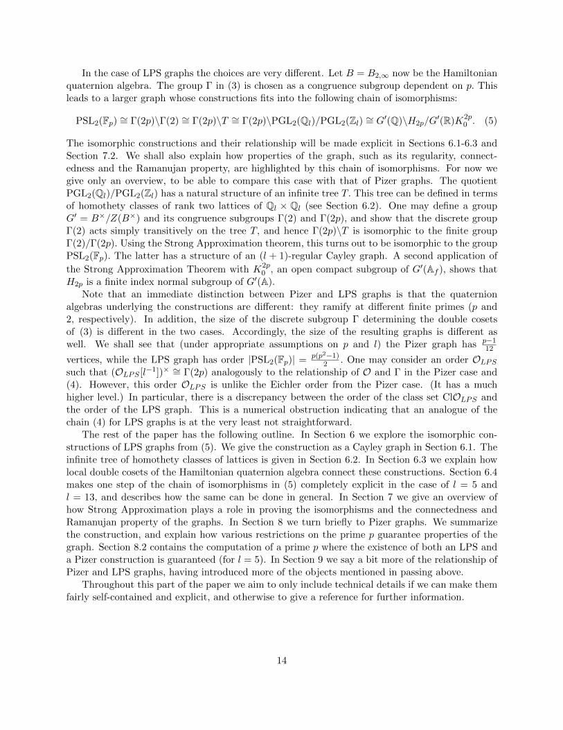
In the case of LPS graphs the choices are very different. Let B = B2,∞ now be the Hamiltonianquaternion algebra. The group Γ in (3) is chosen as a congruence subgroup dependent on p. Thisleads to a larger graph whose constructions fits into the following chain of isomorphisms:

PSL2(Fp) ∼= Γ(2p)\Γ(2) ∼= Γ(2p)\T ∼= Γ(2p)\PGL2(Ql)/PGL2(Zl) ∼= G′(Q)\H2p/G′(R)K2p

0 . (5)

The isomorphic constructions and their relationship will be made explicit in Sections 6.1-6.3 andSection 7.2. We shall also explain how properties of the graph, such as its regularity, connect-edness and the Ramanujan property, are highlighted by this chain of isomorphisms. For now wegive only an overview, to be able to compare this case with that of Pizer graphs. The quotientPGL2(Ql)/PGL2(Zl) has a natural structure of an infinite tree T. This tree can be defined in termsof homothety classes of rank two lattices of Ql × Ql (see Section 6.2). One may define a groupG′ = B×/Z(B×) and its congruence subgroups Γ(2) and Γ(2p), and show that the discrete groupΓ(2) acts simply transitively on the tree T, and hence Γ(2p)\T is isomorphic to the finite groupΓ(2)/Γ(2p). Using the Strong Approximation theorem, this turns out to be isomorphic to the groupPSL2(Fp). The latter has a structure of an (l + 1)-regular Cayley graph. A second application of

the Strong Approximation Theorem with K2p0 , an open compact subgroup of G′(Af ), shows that

H2p is a finite index normal subgroup of G′(A).Note that an immediate distinction between Pizer and LPS graphs is that the quaternion

algebras underlying the constructions are different: they ramify at different finite primes (p and2, respectively). In addition, the size of the discrete subgroup Γ determining the double cosetsof (3) is different in the two cases. Accordingly, the size of the resulting graphs is different aswell. We shall see that (under appropriate assumptions on p and l) the Pizer graph has p−1

12

vertices, while the LPS graph has order |PSL2(Fp)| = p(p2−1)2 . One may consider an order OLPS

such that (OLPS [l−1])× ∼= Γ(2p) analogously to the relationship of O and Γ in the Pizer case and(4). However, this order OLPS is unlike the Eichler order from the Pizer case. (It has a muchhigher level.) In particular, there is a discrepancy between the order of the class set ClOLPS andthe order of the LPS graph. This is a numerical obstruction indicating that an analogue of thechain (4) for LPS graphs is at the very least not straightforward.

The rest of the paper has the following outline. In Section 6 we explore the isomorphic con-structions of LPS graphs from (5). We give the construction as a Cayley graph in Section 6.1. Theinfinite tree of homothety classes of lattices is given in Section 6.2. In Section 6.3 we explain howlocal double cosets of the Hamiltonian quaternion algebra connect these constructions. Section 6.4makes one step of the chain of isomorphisms in (5) completely explicit in the case of l = 5 andl = 13, and describes how the same can be done in general. In Section 7 we give an overview ofhow Strong Approximation plays a role in proving the isomorphisms and the connectedness andRamanujan property of the graphs. In Section 8 we turn briefly to Pizer graphs. We summarizethe construction, and explain how various restrictions on the prime p guarantee properties of thegraph. Section 8.2 contains the computation of a prime p where the existence of both an LPS anda Pizer construction is guaranteed (for l = 5). In Section 9 we say a bit more of the relationship ofPizer and LPS graphs, having introduced more of the objects mentioned in passing above.

Throughout this part of the paper we aim to only include technical details if we can make themfairly self-contained and explicit, and otherwise to give a reference for further information.

14

5 Background on Ramanujan graphs and adeles

In this section we fix notation and review some definitions and facts that we will be using for theremainder of Part 2.

Expander graphs are graphs where small sets of vertices have many neighbors. For manyapplications of expander graphs, such as in Part 1, one wants (l + 1)-regular expander graphs Xwith l small and the number of vertices of X large. If X is an (l+1)-regular graph (i.e. where everyvertex has degree l+ 1), then l+ 1 is an eigenvalue of the adjacency matrix of X. All eigenvalues λsatisfy −(l+ 1) ≤ λ ≤ (l+ 1), and −(l+ 1) is an eigenvalue if and only if X is bipartite. Let λ(X)be the second largest eigenvalue in absolute value of the adjacency matrix. The smaller λ(X) is,the better expander X is. Alon–Boppana proved that for an infinite family of (l+1)-regular graphsof increasing size, lim inf(X) λ(X) ≥ 2

√l [Alo86]. An (l + 1)-regular graph X is called Ramanujan

if λ(X) ≤ 2√l. Thus an infinite family of Ramanujan graphs are optimal expanders.

For a finite prime p, let Qp denote the field of p-adic numbers and Zp its ring of integers. LetQ∞ = R. We denote the adele ring of Q by A and recall that it is defined as a restricted directproduct in the following way,

A =∏′

p

Qp =

{(ap) ∈

∏p

Qp : ap ∈ Zp for all but a finite number of p <∞

}.

We denote the ring of finite adeles by Af , that is

Af =∏′

p<∞Qp =

{(ap) ∈

∏p<∞

Qp : ap ∈ Zp for all but a finite number of p

}.

Let A× denote the idele group of Q, the group of units of A,

A× =∏′

p

Qp =

{(ap) ∈

∏p

Q×p : ap ∈ Z×p for all but a finite number of p <∞

}.

Let B be a quaternion algebra over Q, B× the invertible elements of B and O an order of B.For a prime p let Op = O ⊗Z Zp. Then let

B×(A) =∏′

p

B×(Qp) =

{(gp) ∈

∏p

B×(Qp) : gp ∈ O×p for all but a finite number of p <∞

}.

More generally for an indexed set of locally compact groups {Gv}v∈I with a correspondingindexed set of compact open subgroups {Kv}v∈I we may define the restricted direct product of theGv with respect to the Kv by the following

G :=∏′

v∈IGv =

{(gv) ∈

∏v∈I

Gv : gv ∈ Kv for all but a finite number of v

}.

If we define a neighborhood base of the identity as{∏v

Uv : Uv neighborhood of identity in Gv and Uv = Kv for all but a finite number of v

}then G is a locally compact topological group.

15

6 LPS Graphs

We describe the LPS graphs used in [CGL06] for a proposed hash function. They were firstconsidered in [LPS88], for further details see also [Lub10]. We shall examine the objects andisomorphisms in (5) in more detail. We review constructions of these graphs in turn as Cayley graphsand graphs determined by rank two lattices or, equivalently, local double cosets. Throughout thissection, let l and p be distinct, odd primes both congruent to 1 modulo 4. We shall give constructionsof (l+1)-regular Ramanujan graphs whose size depends on p. We shall also assume for convenience2

that(pl

)= 1, i.e. that p is a square modulo l.

6.1 Cayley graph over Fp.

This description follows [LPS88, Section 2]. The graph we are interested in is the Cayley graphof the group PSL2(Fp). We specify a set of generators S below. The vertices of the graph are thep(p2−1)

2 elements of PSL2(Fp). Two vertices g1, g2 ∈ PSL2(Fp) are connected by an edge if and onlyif g2 = g1h for some h ∈ S.

Next we give the set of generators S. Since l ≡ 1 mod 4 it follows from a theorem of Jacobi[Lub10, Theorem 2.1.8] that there are l + 1 integer solutions to

l = x20 + x2

1 + x22 + x2

3; 2 - x0; x0 > 0. (6)

In this case we will also have 2|xi for all i > 0. Let S be the set of solutions of (6). Since p ≡ 1

mod 4 we have(−1p

)= 1. Let ε ∈ Z such that ε2 ≡ −1 mod p. Then to each solution of (6) we

assign an element of PGL2(Z) as follows:

(x0, x1, x2, x3) 7→(

x0 + x1ε x2 + x3ε−x2 + x3ε x0 − x1ε

). (7)

Note that the matrix on the right-hand side has determinant l mod p. Since(lp

)= 1 this deter-

mines an element of PSL2(Fp). The l + 1 elements of PSL2(Fp) determined by (7) form the setof Cayley generators. Let us abuse notation and denote this set with S as well. This graph isconnected. To prove this fact, one may use the theory of quadratic Diophantine equations [LPS88,Proposition 3.3]. Alternately, the chain of isomorphisms (5) proves this fact by relating this Cayleygraph to a quotient of a connected graph [Lub10, Theorem 7.4.3]: the infinite tree we shall describein the next section.

The solutions (x0, x1, x2, x3) and (x0,−x1,−x2,−x3) correspond to elements of S that are in-verses in PSL2(Fp). Since |S| = l + 1 this implies that the generators determine an undirected(l + 1)-regular graph.

6.2 Infinite tree of lattices

Next we shall work over Ql. We give a description of the same graph in two ways: in terms ofhomothety classes of rank two lattices, and in terms of local double cosets of the multiplicative group

2If p is not a square modulo l, then the constructions described below result in bipartite Ramanujan graphs withtwice as many vertices.

16

of the Hamiltonian quaternion algebra. The description follows [Lub10, 5.3, 7.4]. Let B = B2,∞ bethe Hamiltonian quaternion algebra defined over Q.

First we review the construction of an (l+ 1)-regular infinite tree on homothety classes of ranktwo lattices in Ql × Ql following [Lub10, 5.3]. The vertices of this infinite graph are in bijectionwith PGL2(Ql)/PGL2(Zl). To talk about a finite graph, we shall then consider two subgroups Γ(2)and Γ(2p) in B×/Z(B×). It turns out that Γ(2) acts simply transitively on the infinite tree, andorbits of Γ(2p) on the tree are in bijection with the finite group Γ(2)/Γ(2p). Under our assumptionsthe latter turns out to be in bijection with PSL2(Fp) above and the finite quotient of the tree isisomorphic to the Cayley graph above.

First we describe the infinite tree following [Lub10, 5.3]. Consider the two dimensional vectorspace Ql × Ql with standard basis e1 = t〈1, 0〉, e2 = t〈0, 1〉. A lattice is a rank two Zl-submoduleL ⊂ Ql×Ql. It is generated (as a Zl-module) by two column vectors u,v ∈ Ql×Ql that are linearlyindependent over Ql. We shall consider homothety classes of lattices, i.e. we say lattices L1 andL2 are equivalent if there exists an 0 6= α ∈ Ql such that αL1 = L2. Writing u,v in the standardbasis e1, e2 maps the lattice L to an element ML ∈ GL2(Ql). Let u1,v1,u2,v2 ∈ Ql × Ql and letLi = SpanZl

{ui,vi} (i = 1, 2) be the lattices generated by these respective pairs of vectors, withML1 and ML2 the corresponding matrices. Let M ∈ GL2(Ql) so that ML1M = ML2 . Then L1 = L2

(as subsets of Ql×Ql) if and only if M ∈ GL2(Zl). It follows that the homothety classes of latticesare in bijection with PGL2(Ql)/PGL2(Zl). Equivalently, we may say that PGL2(Ql)/PGL2(Zl) actssimply transitively on homothety classes of lattices.

The vertices of the infinite graph T are homothety classes of lattices. The classes [L1], [L2]are adjacent in T if and only if there are representatives L′i ∈ [Li] (i = 1, 2) such that L′2 ⊂ L′1and [L′1 : L′2] = l. We show that this relation defines an undirected (l + 1)-regular graph. By thetransitive action of GL2(Ql) on lattices we may assume that L′1 = Zl × Zl = SpanZl

{e1, e2}, thestandard lattice and L′2 ⊂ Zl × Zl. The map Zl → Zl/lZl ∼= Fl induces a map from Zl × Zl to F2

l .Since the index of L′2 in Zl × Zl is l, the image of L′2 is a one-dimensional vector subspace of F2

l .This implies that L′2 ⊃ {le1, le2}, i.e. L′2 ⊃ lL′1 and the graph is undirected.3 Furthermore, sincethere are l + 1 one-dimensional subspaces of F2

l , the graph is (l + 1)-regular.The l+1 neighbors of the standard lattice can be described explicitly by the following matrices:

Ml =

(1 00 l

), Mh =

(l h0 1

)for 0 ≤ h ≤ l − 1 (8)

For any of the matrices Mt (0 ≤ t ≤ l) the columns of Mt span a different one-dimensional subspaceof Fl×Fl. The matrices determine the neighbors of any other lattice by a change of basis in Ql×Ql.

By the above we can already see that T is isomorphic to the graph on PGL2(Ql)/PGL2(Zl) withedges corresponding to multiplication by generators (8) above. To show that T is a tree it sufficesto show that there is exactly one path from the standard lattice Zl × Zl to any other homothetyclass. This follows from the uniqueness of the Jordan–Holder series in a finite cyclic l-group as in[Lub10, p. 69].

In the next section, we show that the above infinite tree is isomorphic to a Cayley graph of asubgroup of B×/Z(B×). In Section 6.4 we give an explicit bijection between the Cayley generatorsand the matrices given in (8) above.

3I.e. the adjacency relation defined above is symmetric.

17

6.3 Hamiltonian quaternions over a local field

To turn the above infinite tree into a finite, (l + 1)-regular graph we shall define a group actionon its vertices. Let B be the algebra of Hamiltonian quaternions defined over Q. Let G′ be theQ-algebraic group B×/Z(B×). In this subsection we shall follow [Lub10, 7.4] to define normalsubgroups Γ(2p) ⊂ Γ(2) of Γ = G′(Z[l−1]) such that Γ(2) acts simply transitively on the graphT. The quotient Γ(2p)\T will be isomorphic to the Cayley graph of the finite quotient groupΓ(2)/Γ(2p). This graph is isomorphic to the Cayley graph of PSL2(Fp) defined in Section 6.1above. Thus we have the following equation.

PSL2(Fp) ∼= Γ(2p)\Γ(2) ∼= Γ(2p)\T ∼= Γ(2p)\PGL2(Ql)/PGL2(Zl). (9)

We first define the groups Γ, Γ(2), Γ(2p) and then examine their relationship with T. Recall thatB = B2,∞, i.e. B is ramified at 2 and∞. For a commutative ring R define B(R) = SpanR{1, i, j,k}where i2 = j2 = −1 and ij = −ji = k. We introduce the notation bx0,x1,x2,x3 := x0 +x1i+x2j+x3k.Recall that for b = bx0,x1,x2,x3 we may define b = bx0,−x1,−x2,−x3 and the reduced norm of b asN(b) = bb = x2

0 +x21 +x2

2 +x23. For a (commutative, unital) ring R an element b ∈ B(R) is invertible

in B(R) if and only if N(b) is invertible in R. (Then b−1 = (N(b))−1b.) Furthermore

[bx0,x1,x2,x3 , by0,y1,y2,y3 ] = 2(x2y3 − x3y2)i + 2(x3y1 − x1y3)j + 2(x1y2 − x2y1)k, (10)

and hence ifR has no zero divisors then Z(B(R)) = R. In particular Z(B×(Z[l−1])) = {±lk | k ∈ Z}.Recall that S was the set of l+ 1 integer solutions of (6). Any solution x0, x1, x2, x3 determines

a b = bx0,x1,x2,x3 ∈ B(Z[l−1]) such that N(b) = l. Since l is invertible in Z[l−1] we in fact haveb ∈ B×(Z[l−1]). Let Γ = G′(Z[l−1]) = B×(Z[l−1])/Z(B×(Z[l−1])) and let us denote the image ofS in Γ by S as well. Since B×(Z[l−1]) = {b ∈ B(Z[l−1]) | N(b) = lk, k ∈ Z}, if [b] ∈ Γ forb ∈ B×(Z[l−1]) then it follows from [Lub10, Corollary 2.1.10] that b is a unit multiple of an elementof 〈S〉. It follows that Γ = 〈S〉{[1], [i], [j], [k]} and the index of 〈S〉 in Γ is 4. In fact observe that ifb ∈ S then b−1 ∈ S and [Lub10, Corollary 2.1.11] states that 〈S〉 is a free group on l+1

2 generators.We shall see that 〈S〉 agrees with a congruence subgroup Γ(2).

Now let N = 2M be coprime to l and let R = Z[l−1]/NZ[l−1]. The quotient map Z[l−1] → Rdetermines a map B(Z[l−1])→ B(R). This restricts to a map B×(Z[l−1])→ B×(R). Observe thatif M = 1 then B×(R) is commutative. If M = p then the subgroup

Z :={bx0,0,0,0 ∈ B×(Z[l−1]/2pZ[l−1]) | p - x0, 2 - x0

}(cf. [LPS88, p. 266]) is central in B×(R). Consider the commutative diagram:

B(Z[l−1])× −→ B×(Z[l−1]/2Z[l−1]) −→ B×(Z[l−1]/2pZ[l−1])↓ ↓ ↓Γ

π2−→ B×(Z[l−1]/2Z[l−1])πp−→ B×(Z[l−1]/2pZ[l−1])/Z

(11)

and define4 π2p := πp ◦ π2 and Γ(2) := kerπ2 and Γ(2p) = kerπ2p. Observe that by the congruenceconditions (cf. (6)) S ⊆ Γ is contained in Γ(2) and in fact 〈S〉 = Γ(2) ⊇ Γ(2p). As mentioned abovethis implies that Γ(2) is a free group with l+1

2 generators.

4The definition here agrees with the choices in [LPS88] as well as Γ(N) = ker(G′(Z[l−1]) → G′(Z[l−1]/NZ[l−1]))in [Lub10]. Here G′ = B×/Z(B×) as a Q-algebraic group. Note however that by (10) the center Z(B×(R)) forR = Z[l−1]/NZ[l−1], N = 2M may not be spanned by 1 + NZ[l−1]. In fact from (10) B×(R) is commutative forM = 1 and for M = p we have Z(B×(R)) = Z ⊕ [p]i + [p]j + [p]k. However the image of 〈S〉 in B×(R) is trivial ifM = 1 and intersects the center in Z when M = p.

18

To see the action of Γ(2) on T note that B splits over Ql and hence B(Ql) ∼= M2(Ql). Since−1 ∈ (F×l )2 there exists an ε ∈ Zl such that ε2 = −1. Then we have an isomorphism σ : B(Ql) →M2(Ql) [Lub10, p. 95] given by

σ(x0 + x1i + x2j + x3k) =

(x0 + x1ε x2 + x3ε−x2 + x3ε x0 − x1ε

). (12)

Observe that σ(B×(Z[l−1])) ⊆ GL2(Ql) and σ maps elements of the center into scalar matrices,and hence this defines an action of Γ (and hence Γ(2),Γ(2p)) on T. This action preserves the graphstructure. Then we have the following. Observe that σ maps the elements of 〈S〉 ⊆ Γ into thecongruence subgroup of PGL2(Zl) modulo 2.

Proposition 6.1. [Lub10, Lemma 7.4.1] The action of Γ(2) on the tree T = PGL2(Ql)/PGL2(Zl)is simply transitive (and respects the graph structure).

Proof. See loc.cit. for details of the proof. Transitivity follows from the fact that T is connectedand elements of S map a vertex of T to its distinct neighbors. The group Γ(2) = 〈S〉 is a discretefree group, hence its intersection with a compact stabilizer PGL2(Zl) is trivial. This implies thatthe neighbors are distinct and the stabilizer of any vertex is trivial.

The above implies that the orbits of Γ(2p) on T have the structure of the Cayley graphΓ(2)/Γ(2p) with respect to the generators S. We can see from the maps in (11) that Γ(2)/Γ(2p) isisomorphic to a subgroup of G′(Z/2pZ) ∼= G′(Z/2Z) × G′(Z/pZ). (This last isomorphism followsfrom the Chinese Remainder Theorem.) Since the image of Γ(2) in G′(Z/2Z) is trivial, we mayidentify Γ(2)/Γ(2p) with a subgroup of G′(Z/pZ). Here G′(Z/pZ) ∼= PGL2(Fp). (For an explicitisomorphism take an analogue of σ in (12) with ε ∈ Z/pZ such that ε2 = −1.) The image of Γ(2)agrees with PSL2(Fp) as a consequence of the Strong Approximation Theorem [Lub10, Lemma7.4.2]. We shall discuss this in the next section.

We summarize the contents of this section.

Theorem 6.2. [Lub10, Theorem 7.4.3] Let l and p be primes so that l ≡ p ≡ 1 mod 4 and lis a quadratic residue modulo 2p. Let S ⊂ PSL2(Fp) be the (l + 1)-element set corresponding tothe solutions of (6) via the map (7) and Cay(PSL2(Fp), S) the Cayley graph determined by theset of generators S on the group PSL2(Fp). Let T be the graph on PGL2(Ql)/PGL2(Zl) with edgescorresponding to multiplication by elements listed in (8). Let B be the Hamiltonian quaternionalgebra over Q and Γ(2p) the kernel of the map π2p in (11) (a cocompact congruence subgroup).Then Γ(2p) acts on the infinite tree T and we have the following isomorphism of graphs:

Cay(PSL2(Fp), S) ∼= Γ(2p)\PGL2(Ql)/PGL2(Zl). (13)

These are connected, (l + 1) regular, non-bipartite, simple, graphs on p3−p2 vertices.

6.4 Explicit isomorphism between generating sets

We have seen above that the LPS graph can be interpreted as a finite quotient of the infinite treeof homothety classes of lattices. In this case, the edges are given by matrices that take a Zl-basisof one lattice to a Zl-basis of one of its neighbors. On the other hand, the edges can be given interms of the set of generators S. Proposition 6.1 states that 〈σ(S)〉 = Γ(2) ⊂ G′(Z[l−1]) acts simply

19

transitively on the tree T. The proof of the proposition (cf. [Lub10, Lemma 7.4.1]) implicitly showsthat there exists a bijection between elements of σ(S) ⊂ PGL2(Zl) and the matrices given in (8).

In this section we wish to make this bijection more explicit. For a fixed α ∈ S we find the matrixfrom the list (8) determining the same edge of T . As in Section 6.3 we write σ(α) ∈ PGL2(Zl)for the elements of σ(S). This amounts to finding the matrix M from the list in (8) such thatσ(α)−1M ∈ PGL2(Zl).

To pair up matrices from (8) with the corresponding elements of S, we introduce the followingnotation. Let us number the solutions to αα = l as α0, . . . , αl−1, αl so that we have the correspon-dence σ(αh)−1Mh ∈ PGL2(Zl) for 0 ≤ h ≤ l. By giving an explicit correspondence, we mean thatgiven an α ∈ σ−1(S), we determine 0 ≤ h ≤ l such that α = αh.

Elements of σ(S) ⊂ PGL2(Zl) are given in terms of an ε ∈ Zl such that ε2 = −1. Let a, b bethe positive integers such that a2 + b2 = l and a is odd. Let 0 ≤ e ≤ l − 1 so that eb = a. Then inZl we have either ε ∈ e+ lZl and ε−1 = −ε ∈ −e+ lZl or ε ∈ −e+ lZl and ε−1 = −ε ∈ e+ lZl.

Let α = x0 + x1i + x2j + x3k so that σ(α) ∈ S, and a, b, e, ε are as above. Let

αh = x(h)0 + x

(h)1 i + x

(h)2 j + x

(h)3 k

for 0 ≤ h ≤ l. Here x0, x1, x2, x3 are integers; it is convenient to think about them (as well as

x(h)0 , x

(h)1 , x

(h)2 , x

(h)3 for 0 ≤ h ≤ l) as being in Z ⊂ Zl. Then

σ(α)−1 =1

l

(x0 − x1ε −x2 − x3εx2 − x3ε x0 + x1ε

)(14)

and

σ(α)−1 ·(l h0 1

)=

(x0 − x1ε l−1 (h(x0 − x1ε) + (−x2 − x3ε))x2 − x3ε l−1 (h(x2 − x3ε) + (x0 + x1ε))

)σ(α)−1 ·

(1 00 l

)=

(l−1(x0 − x1ε) −x2 − x3εl−1(x2 − x3ε) x0 + x1ε

) (15)

Then by (15) we have that x(l)0 − x

(l)1 ε and x

(l)2 − x

(l)3 ε are in lZl. Hence x

(l)0 ∈ x

(l)1 ε + lZl,

and thus (x(l)0 )2 ∈ (x

(l)1 ε)2 + lZl = −x2

1 + lZl, whence (x(l)0 )2 + (x

(l)1 )2 ∈ lZl. Note that since

(x(l)0 )2 + (x

(l)1 )2 + (x

(l)2 )2 + (x

(l)3 )2 = l and x0 is positive, this implies that (x

(l)0 )2 + (x

(l)1 )2 = l and

(x(l)2 )2 + (x

(l)3 )2 = 0, i.e. x

(l)2 = x

(l)3 = 0 and x

(l)0 = a, |x(l)

1 | = b. Note that by the assumptions inSection 6.1, a± bi, a± bj, a± bk ∈ S. A straightforward computation now shows the following.

ε ∈ e+ lZl ⇒ αl = a+ bi, α0 = a− bi, αe = a− bj, αl−e = a+ bj, α1 = a− bk, αl−1 = a+ bk

ε ∈ −e+ lZl ⇒ αl = a− bi, α0 = a+ bi, αe = a− bj, αl−e = a+ bj, α1 = a+ bk, αl−1 = a− bk(16)

Now let us assume that for α = x0 + x1i + x2j + x3k we have that x0 − x1ε /∈ lZl. This impliesthat It remains to determine the h such that α = αh when α is not one of the solutions covered by(16). In that case, we may assume h /∈ {0, 1, e, l − e, l − 1, l} and we have

h(x0 − x1ε) + (−x2 − x3ε) ∈ lZl; (17)

h(x2 − x3ε) + (x0 + x1ε) ∈ lZl. (18)

20

A straightforward computation based on αα = l shows that (17) and (18) are satisfied by the sameelement in Fl = Z/lZ. The element

h =x2 + x3ε

x0 − x1ε∈ Fl (19)

is well defined, since x0 − x1ε /∈ lZl, furthermore, it uniquely determines an 0 ≤ h ≤ l. For a fixedα not covered by (16), one may thus find h such that α = αh.

We give two explicit examples.

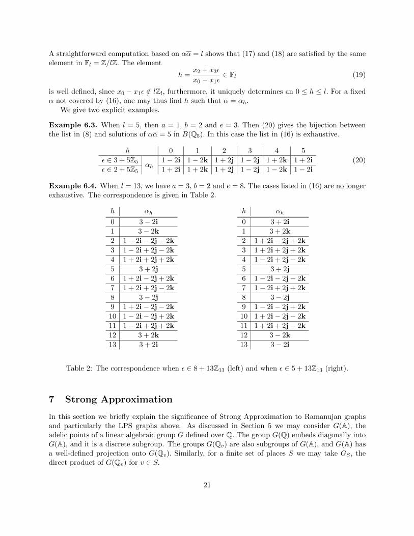
Example 6.3. When l = 5, then a = 1, b = 2 and e = 3. Then (20) gives the bijection betweenthe list in (8) and solutions of αα = 5 in B(Q5). In this case the list in (16) is exhaustive.

h 0 1 2 3 4 5

ε ∈ 3 + 5Z5 αh1− 2i 1− 2k 1 + 2j 1− 2j 1 + 2k 1 + 2i

ε ∈ 2 + 5Z5 1 + 2i 1 + 2k 1 + 2j 1− 2j 1− 2k 1− 2i

(20)

Example 6.4. When l = 13, we have a = 3, b = 2 and e = 8. The cases listed in (16) are no longerexhaustive. The correspondence is given in Table 2.

h αh

0 3− 2i

1 3− 2k

2 1− 2i− 2j− 2k

3 1− 2i + 2j− 2k

4 1 + 2i + 2j + 2k

5 3 + 2j

6 1 + 2i− 2j + 2k

7 1 + 2i + 2j− 2k

8 3− 2j

9 1 + 2i− 2j− 2k

10 1− 2i− 2j + 2k

11 1− 2i + 2j + 2k

12 3 + 2k

13 3 + 2i

h αh

0 3 + 2i

1 3 + 2k

2 1 + 2i− 2j + 2k

3 1 + 2i + 2j + 2k

4 1− 2i + 2j− 2k

5 3 + 2j

6 1− 2i− 2j− 2k

7 1− 2i + 2j + 2k

8 3− 2j

9 1− 2i− 2j + 2k

10 1 + 2i− 2j− 2k

11 1 + 2i + 2j− 2k

12 3− 2k

13 3− 2i

Table 2: The correspondence when ε ∈ 8 + 13Z13 (left) and when ε ∈ 5 + 13Z13 (right).

7 Strong Approximation

In this section we briefly explain the significance of Strong Approximation to Ramanujan graphsand particularly the LPS graphs above. As discussed in Section 5 we may consider G(A), theadelic points of a linear algebraic group G defined over Q. The group G(Q) embeds diagonally intoG(A), and it is a discrete subgroup. The groups G(Qv) are also subgroups of G(A), and G(A) hasa well-defined projection onto G(Qv). Similarly, for a finite set of places S we may take GS , thedirect product of G(Qv) for v ∈ S.

21

Strong Approximation (when it holds) is the statement that for a group G and a finite set ofplaces S the subgroup G(Q)GS is dense in G(A). This implies that

G(A) = G(Q)GSK for any open subgroup K ≤ G(A). (21)

For example, Strong Approximation holds for G = SL2 and any set of places S = {v}. However,in the form written above it does not hold for GL2 or PGL2. However one can prove results similarto (21) for GL2 adding restrictions on the subgroup K:

G(A) = G(Q)GSK for an open subgroup K ≤ G(A) if K is “sufficiently large.” (22)

Here we shall haveK =

∏v/∈S

Kv; Kv ≤ G(Zv) (23)

and the condition of being “sufficiently large” can be made precise by requiring that the determinantmap det : Kv → Z×v be surjective for all v 6∈ S.

Strong Approximation holds for the algebraic group of elements of a quaternion algebra of unitnorm [Vig80, Theoreme 4.3]. We shall use this statement to prove a statement like (22) for thealgebraic group of invertible quaternions. A similar statement then holds for G′ = B×/Z(B×) anda subgroup K ′ that is not quite “large enough.” The implications for Pizer graphs and LPS graphswill be discussed in Sections 7.2 and 7.3 below.

These statements coming from Strong Approximation are crucial for proving that the variousconstructions produce Ramanujan graphs. As seen in Section 5 the Ramanujan property of agraph can be expressed in terms of its eigenvalues. Given a graph (constructed e.g. via local doublecosets as seen above) the Strong Approximation theorem can be used to relate its spectrum to therepresentation theory of G(A). In that context a theorem of Deligne resolves the issue by provinga special case of the Ramanujan conjecture (see [Lub10, Theorem 6.1.2, Theorem A.1.2, TheoremA.2.14] and [Del71]).

7.1 Approximation for invertible quaternions

The argument below is adapted from [Gel75, Section 3] and [Lub10, 6.3].5

Let B be a (definite) quaternion algebra over Q, B× its invertible elements and B1 = {b ∈B | N(b) = 1} its elements of reduced norm 1, recall N(b) = bb. Let l be a prime where B issplit. Then by [Vig80, Theoreme 4.3] we have that B1(Q)B1(Ql) is dense in B1(A) thus B1(A) =B1(Q)B1(Ql)K for any open subgroup K ≤ B1(A). An open subgroup K ≤ B1(A) is of the formK =

∏vKv where Kv ≤ B1

v is open and Kv = B1(Zv) for all but finitely many places v. It follows

that given any open subgroups K(B1)v ≤ B1(Zv) (v 6= l) such that K

(B1)v = B1(Zv) for all but

finitely many places v we have that

B1(A) = B1(Q)B1(Ql)∏v 6=l

K(B1)v . (24)

To make a similar statement for B× it will be necessary to impose a restriction on the opensubgroups Kv.

5In fact, since at every split place v we have B×(Qv) ∼= GL2(Qv) with the reduced norm on B× corresponding tothe determinant on GL2 [Vig80, p. 3] this is the “same argument at all but finitely many places.”

22

Theorem 7.1. Let Kv ≤ B×(Zv) for every place l 6= v < ∞ so that Kv = B×(Zv) for all butfinitely many v, and the norm map N : Kv → Zv× is surjective for every place v. Then

B×(A) = B×(Q)B×(R)B×(Ql)∏

l 6=v<∞Kv. (25)

Note that by [Voi18, Lemma 13.4.6] the norm map N : B×(Zv) → Zv× is surjective for everynonarchimedean v.

Proof. Let b ∈ B×(A), we need to show b is contained on the right-hand side. To write b as aproduct according to the right-hand side of (25) we shall use (24), strong approximation for B1.Observe first that it suffices to show that any b ∈ B×(A) can be written as

b = rhk, where r ∈ B×(Q), h ∈ B1(A), and k ∈ B×(R)B×(Ql)∏

l 6=v<∞Kv. (26)

This is because the intersections Kv∩B1(Qv) are open subgroups of B1(Zv) (and B×(Zv)∩B1(Zv) =

B1(Zv) at all but finitely many places). It thus follows from (24) (choosing K(B1)v := Kv ∩B1(Qv))

that the factor h ∈ B1(A) ⊆ B×(A) from (26) is contained on the right-hand side of (25). It followsthat then b = rhk is contained on the right-hand side of (25) as well. (Note that here the factorsof h and k belonging to different components B×(Qv) commute.)

So we must show that any b ∈ B×(A) decomposes as in (26). Let b = (bv)v for bv ∈ B×(Qv)and set nv := N(bv). For all but finitely many places v we have bv ∈ B×(Zv) and hence nv ∈ Zv×.At a finite set T of finite places we may write nv ∈ vmvZv×. Let us take

nQ =∏v∈T

vmv . (27)

Then nQ ∈ Q>0, nQ ∈ Zv× for every v /∈ T, v <∞ and hence n−1Q nv ∈ Zv× for every finite place v.

It is a fact that there is an r ∈ B×(Q) such that N(r) = nQ. Then for this r we have that thenorm of r−1b ∈ B×(A) is in Zv× for every finite place v.

Let us write (r−1b)v for the component of r−1b ∈ B×(A) at a place v. There exists a k ∈B×(R)B×(Ql)

∏l 6=v<∞Kv, k = (kv)v such that kl = (r−1b)l and k∞ = (r−1b)∞ and N(kv) =

N((r−1b)v) every other place. This follows from the fact that the norm map N : Kv → Zv× issurjective.

Now let h = r−1bk−1. We show h ∈ B1(A). Write h = (hv)v for hv ∈ B×(Qv). It follows fromthe choice of k that hl and h∞ are the identity element of B×(Ql) and B×(R) respectively, andN(hv) = 1 at every other place v. This implies that indeed h ∈ B1(A). This completes the proofthat a decomposition as in (26) exists, and in turn the proof of (25).

7.2 Strong Approximation for LPS graphs

This section is based on [Lub10, 6.3]. (In particular, we recall and elaborate on the proof of thefirst statements in [Lub10, Proposition 6.3.3] in the special case when N = 2p. This is relevant tounderstanding the last step in (5).) We apply a similar formula to (25) with a particular choice ofopen subgroups K ′v to prove a statement that relates double cosets such as in (9) to adelic doublecosets. Let B = B2,∞ be the algebra of Hamiltonian quaternions, ramified at 2 and∞. Recall from

23

Section 6.3 that G′ is the Q-algebraic group B×/Z(B×). Let us fix the prime l ≡ 1 mod 4 as inSection 6. In a similar manner to the proof of (25) is follows that

G′(A) = G′(Q)G′(R)G′(Ql)∏

l 6=v<∞G′(Zv). (28)

Recall that since B splits at l we have G′(Ql) ∼= PGL2(Ql). We wish to have a statement similarto (28) above, replacing G′(Zv) at v = 2 and v = p by congruence subgroups K ′2 and K ′p. (This p isthe one fixed above in Section 6.) Then isomorphism will no longer hold, but the right-hand sidewill be a finite index normal subgroup of G′(A).

The choice of the smaller subgroups K ′2 and K ′p is as follows. For v ∈ {2, p} let

K ′v = ker(G′(Zv)→ G′(Zv/vZv)

). (29)

Here Zv/vZv = Fv is a finite field, hence G′(Zv/vZv) is finite. It follows that the index [Kv : K ′v]is finite. In fact since B2,∞ splits over p we have that G′(Zp/vZp) ∼= PGL2(Fp), hence [Kp : K ′p] =p(p2 − 1). At v = 2 we have G′(F2) = B×(F2) hence [K2 : K ′2] = 8.

Let us set K ′v as above if v ∈ {2, p} and K ′v = Kv = G′(Zv) otherwise, and let us define

H2p :=

G′(Q)G′(R)G′(Ql)∏

l 6=v<∞K ′v

. (30)

By [Lub10, Proposition 6.3.3] Strong Approximation proves that H2p is a finite index normalsubgroup of G′(A).

From the definition of H2p in equation (30) we have a surjection from

G′(Ql)→ G′(Q)\H2p/G′(R)

∏l 6=v<∞

K ′v.

If gl and g′l ∈ G′(Ql) are mapped to the same coset on the right hand side then there existsgq ∈ G′(Q), gr ∈ G′(R) and k =

∏l 6=v<∞ kv ∈

∏l 6=v<∞K

′v such that gl = gqg

′lgrk. This is

equivalent to saying gl = gqg′l and gq ∈ K ′v for all l 6= v < ∞. By the definitions of the K ′vs this

last condition implies gq ∈ Γ(2p). Thus we see that

Γ(2p)\G′(Ql)/G′(Zl) ∼= G′(Q)\H2p/G

′(R)∏v<∞

K ′v. (31)

Strong approximation in the manner discussed above is used to prove that LPS graphs areRamanujan. First one shows that the finite (l+1)-regular graph Γ(2p)\T is Ramanujan if and onlyif all irreducible infinite-dimensional unramified unitary representations of PGL2(Ql) that appearin L2(PGL2(Ql)/Γ(2p)) are tempered [Lub10, Corollary 5.5.3]. Then by the isomorphism abovewhich follows from Strong Approximation, one can extend a representation ρ′l of PGL2(Ql) to anautomorphic representation ρ′ of G′(A) in L2(G′(Q)\G′(A)). By the Jacquet–Langlands correspon-dence, ρ′ corresponds to a cuspidal representation ρ of PGL2(A) in L2(PGL2(Q)\PGL2(A)) suchthat ρv is discrete series for all v where B ramifies (so in our case, 2 and∞) [Lub10, Theorem 6.2.1].Finally, Deligne has proved the Ramanujan–Peterson conjecture in this case of holomorphic mod-ular forms [Lub10, Theorem 6.1.2], [Del71], [Del74] which says that for ρ a cuspidal representationof PGL2(A) in L2(PGL2(Q)\PGL2(A)) with ρ∞ discrete series, ρl is tempered [Lub10, Theorems7.1.1 and 7.3.1]. Under the Jacquet–Langlands correspondence, the adjacency matrix of our graphX corresponds to the Hecke operator Tl [Lub10, 5.3] and the Ramanujan conjecture is equivalentto saying that |λ| ≤ 2

√l for all of its eigenvalues λ 6= ±(l + 1).

24

7.3 Strong Approximation for Pizer graphs

Now we turn to discussing how strong approximation is useful in establishing the bijections in (4).In Section 8 we will discuss Pizer’s construction of Ramanujan graphs. These graphs are isomorphicto supersingular isogeny graphs. Their vertex set is the class group of a maximal order O in thequaternion algebra Bp,∞. This set is in bijection with an adelic double coset space, which in turnis in bijection with a set of local double cosets.

Let B = Bp,∞ be a quaternion algebra (over Q) ramified exactly at ∞ and at a finite primep. At every finite prime v, B(Qv) has a unique maximal order up to conjugation [Vig80, Lemme1.4]. Given a maximal order O of B, one may define the adelic group B×(Af ) as a restricted directproduct of the groups B×(Qv) over the finite places, with respect to O×v . (Recall that this meansthat any element of B×(Af ) is a vector indexed by the finite places v; the component at v is inB×(Qv) and in fact in O×v at all but finitely many places.) This adelic object does not in factdepend on the choice of the maximal ideal O. In particular, at any prime l 6= p where B splits wehave B×(Ql) ∼= GL2(Ql) and O×l ∼= GL2(Zl).

Let us now fix a prime l where B splits. The same argument as in Section 7.1 works restrictedto B×(Af ) (the finite adeles). It follows that we have

B×(Af ) = B×(Q)B×(Ql)∏

l 6=v<∞B×(Zv). (32)

Proposition 7.2. We have the bijections (cf. [CGL09, (1)])

B×(Q)\B×(Af )/∏v<∞

B×(Zv) ∼=(O(Z[l−1]))×\B×(Ql)/B×(Zl)

∼=(O(Z[l−1]))×\GL2(Ql)/GL2(Zl).(33)

Proof. The first bijection follows from (32) and an argument similar to the proof of (31). Indeed,(32) implies that there is a surjection

B×(Ql)→ B×(Q)\B×(Af )/∏

l 6=v<∞B×(Zv). (34)

Now two elements gl, g′l ∈ B×(Ql) land in the same double coset via this bijection if and only

if gl = gqg′lk in B×(Af ). Then gl = gqg

′l (from equality at the place l) and gq ∈ B×(Zv) (from

equality at the places l 6= v < ∞). Consider the element gq ∈ B(Q), for example in terms of itscoordinates in the standard basis {1, i, j,k} of B. Since gq ∈ B×(Zv) we have that gq ∈ O(Z[l−1]),and gq ∈ B×(Ql) implies that in fact gq ∈ (O(Z[l−1]))×. This completes the proof of the firstbijection in (33).

Now the second bijection follows from the fact that B splits at the prime l and hence B×(Ql) ∼=GL2(Ql) with the unique maximal order GL2(Zl).

Finally, we wish to also address the bijection between the adelic double coset object and theclass group of the maximal order O. This fact follows from the fact that ideals of O are locallyprincipal. We omit defining ideals of an order O or defining the class group here and instead referthe reader to [Vig80, §4], [Che10, §2.3] or [Voi18]. For the statement about the bijection betweenthe class group Cl(O) and the adelic double cosets in (33) above, see for example [Che10, Theorem2.6].

25

8 Pizer Graphs

In this section we give an overview of Pizer’s [Piz98] construction of a Ramanujan graph. Thegraphs constructed by Pizer are isomorphic to the graphs of supersingular elliptic curves over Fp2[CGL09, Section 2]. These graphs were considered by Mestre [Mes86] and Ihara [Iha66] before (cf.[JMV05]), but Pizer’s construction reveals their connection to quaternion algebras, proving theirRamanujan property. In Section 9 we shall compare the resulting graphs to the LPS constructiondescribed above.

Pizer’s description is in terms of a quaternion algebra and a pair of prime parameters p, l. Weshall aim to keep technical details to a minimum, and focus on the choice of quaternion algebra andparameters. This elucidates the connection with the LPS construction. Recall that the meaningof the parameters is similar in both cases: the resulting graphs are (l + 1)-regular and their sizedepends on the value of p. Varying p (subject to some constraints) produces an infinite familyof (l + 1)-regular Ramanujan graphs. However, we shall see that the constraints imposed on theparameters {p, l} by the LPS and Pizer constructions do not agree. In Section 8.2 we give anexplicit comparison between the admissible values of the parameter p in the example when l = 5.

First we wish to summarize the construction via Pizer [Piz98]. In particular we wish to explainthe elements of [Piz98, Theorem 5.1]. Details are kept to a minimum; the reader is encouraged toconsult op.cit. for details, in particular [Piz98, 4.]. We mention one feature of Pizer’s approach inadvance: we shall see that here the graph is given via its adjacency matrix. Note that this is of adifferent flavor from the LPS case. There the edges of the graph were specified “locally:” given avertex of the graph (as an element of a group in Section 6.1 or as a class of lattices in Section 6.2),its neighbors were specified directly. (See Section 6.4 for an explicit parametrization of the edgesat a vertex.) In Pizer’s approach the adjacency matrix, a Brandt matrix (associated to an Eichlerorder in the quaternion algebra) specifies the edge structure of the graph.

8.1 Overview of the construction

Let us fix B = Bp,∞ to be the quaternion algebra over Q that is ramified precisely at p and atinfinity. We shall consider orders O of level N = pM and N = p2M in B, where M is coprime top. The vertex set of our graph G(N, l) shall be in bijection with (a subset of) the class group of O.The class number of O depends only on the level of the order and hence we may write H(pM) orH(p2M) for the size of such a graph. In the case where M = 1 by the Eichler class number formula[Piz98, Proposition 4.4] we have:

H(p) =p− 1

12+

1

4

(1−

(−4

p

))+

1

3

(1−

(−3

p

)); (35)

H(p2) =p2 − 1

12+

{0 if p ≥ 543 if p = 3

(36)

where( ··)

is the Kronecker symbol.The vertex set of G(N, l) shall have H(N) elements when N = pM and when N = p2M and

l is a quadratic nonresidue modulo p. (Note that in this case the graph G(p2M, l) is bipartite.)For N = p2M and l a quadratic residue modulo p the graph G(p2M, l) is non-bipartite of sizeH(p2M)

2 . Recall that a similar dichotomy (between bipartite and non-bipartite cases) exists in the

26

LPS construction as well. The following table summarizes the size of G(p, l) and G(p2, l) for the

case where(lp

)= 1 (and p > 3).

p mod 12 H(p) H(p2)2

1 p−112

p2−112

5 p+712

7 p+512

11 p+1312

(37)

The edge structure of the graph G(N, l) is determined via the adjacency matrix. Recall that therows and columns of the adjacency matrix of a graph are indexed by the vertex set. One entry ofthe matrix determines the number of edges between the vertices corresponding to its indices. Theedge structure of G(N, l) is given by a Brandt matrix. There is a space of modular forms associatedto the order O of the quaternion algebra. This space has dimension as in (37) and it carries theaction of a Hecke algebra. For every integer l (coprime to p) the Brandt matrix B(N, l) describesthe explicit action of a particular Hecke operator (Tl) on this space.

Restrictions on the parameters p and l guarantee that B(N, l) is in fact the adjacency matrixof a graph. Properties of the resulting graph (e.g. the graph being simple and connected, as well asstatements about its spectrum and girth) can be phrased as statements about the Brandt matricesB(N, l) and in turn studied as statements about modular forms.

To ensure the edges of the graph G(N, l) are undirected, B(N, l) must be symmetric. By [Piz98,Proposition 4.6] this is the case for N = pM if p ≡ 1 mod 12 and for N = p2M if p > 3.

To ensure the graph has no loops we must have trB(N, l) = 0, and for no multiple edgestr(B(N, l))2 = 0. By [Piz98, Proposition 4.8] these translate to the conditions trB(N, l) = 0,trB(N, l2) = H(N). (This depends on the relationship of the traces within a family of Brandtmatrices B(N, l) for fixed N and varying l.) These traces can be given in terms of parametersdependent on the order O [Piz98, Proposition 4.9].

It turns out that the above conditions together already guarantee that B(N, l) determines aRamanujan graph. This is the content of the following theorem.

Theorem 8.1. [Piz98, Theorem 5.1] Let l be a prime coprime to pM and let N = pM. Considerthe graph G(N, l) determined by the Brandt matrix B(N, l) as its adjacency matrix. Assume thatB(N, l) is symmetric, trB(N, l) = 0 and trB(N, l2) = H(N). Then G(N, l) is a non-bipartite(l + 1)-regular simple Ramanujan graph on H(N) vertices.

Similarly, let N = p2M and assume the above conditions trB(N, l) = 0 and trB(N, l2) = H(N)hold. If l is a quadratic nonresidue modulo p then B(N, l) is the adjacency matrix of a bipartite(l+1)-regular simple Ramanujan graph on H(N) vertices. If l is a quadratic residue modulo p thenB(N, l) is the adjacency matrix of two copies of an (l+ 1)-regular simple non-bipartite Ramanujan

graph on H(N)2 vertices.

Recall that the quaternion algebra B underlying the construction above is ramified at exactlytwo places, p and∞. This uniquely determines the algebra B = Bp,∞ (cf. [Piz98, Proposition 4.1]).Given a specific l one may ask for what p primes and N = p are the conditions trB(N, l) = 0and trB(N, l2) = H(N) satisfied. This can be answered by translating the conditions to modularconditions on p. This is carried out for l = 2 in [Piz98, Example 2]. In the LPS constructionabove we were interested in l + 1 regular graphs where l ≡ 1 mod 4. To compare the families of

27

Ramanujan graphs emerging from the two constructions, in the next section we carry out the samecomputation for l = 5.

8.2 The size of a six-regular Pizer graph

We wish to consider a special case of Pizer’s construction in [Piz98, Section 5] where the orderO is a (level p) maximal order in Bp,∞ and the Ramanujan graph is l + 1 regular. In particular,we are interested in the case where l = 5. (Since the LPS construction discussed in Section 6requires l ≡ 1 mod 4, this is the smallest l where a comparison can be made.) In this section wefollow the methods of [Piz98, Example 2] to give explicit modular conditions on p to satisfy Pizer’sconstruction. The Brandt matrix B(p; 5) associated to the maximal order O ⊂ Bp,∞ (of level p)is a square matrix of size H(p). It follows from Theorem 8.1 [Piz98, Proposition 5.1] that it is theadjacency matrix of a 6-regular simple Ramanujan graph if the following conditions hold:

1. p ≡ 1 mod 12

2. trB(p, 5) = 0

3. trB(p, 52) = ClO

Note that here Condition 1 guarantees that the graph is symmetric, and Condition 2 that it hasno loops. By [Piz98, Proposition 4.4] the condition p ≡ 1 mod 12 gives Cl(O) = MassO = p−1

12 .The Conditions 2 and 3 concern the trace of the Brandt matrices B(p, 5) and B(p, 25) associated

to O of level p. These can be computed using [Piz98, Proposition 4.9]. In particular, loc. cit.guarantees that Conditions 2 and 3 hold under certain conditions. To state these conditions wemust introduce some notation. For m = 5 and m = 25 respectively, let s be an integer such that∆ = s2 − 4m is negative. Let t and r be chosen such that

∆ = s2 − 4 ·m =

{t2r 0 > r ≡ 1 mod 4t24r 0 > r ≡ 2, 3 mod 4

(38)

Let f be any positive divisor of t and d := ∆f2. Let c(s, f, p) denote the number of embeddings of Odp

into Op that are inequivalent modulo the unit group U(Op). By [Piz98, Proposition 4.9] we havethat

Condition 2 is satisfied⇐⇒ c(s, f, p) = 0 for every s, f with m = 5 (39)

Condition 3 is satisfied⇐⇒ c(s, f, p) = 0 for every s, f with m = 52 (40)

The integers c(s, f, p) are given in tables in [Piz76, pp. 692-693]. We use information in these tablesto translate the conditions (39) and (40) into modular conditions on p.

First, if m = 5 the possible values of s,∆, r, t and f are as follows:

s 0 1 2 3 4

∆ −20 −19 −16 −11 −4

t 1 1 2 1 1

r −5 −19 −1 −11 −1

f 1 1 1 2 1 1

d −20 −19 −16 −4 −11 −4

28

It follows from Condition 1 that p - d = ∆f2. It follows from the tables in [Piz76, pp. 692–693] that

c(s, f, p) = c(s, f, p)p2·0+1 = 0 if and only if d is the square of a unit in Zp, i.e. a quadratic residue

modulo p. By Condition 1 we certainly have(−4p

)=(−16p

)= 1 and by quadratic reciprocity(

dp

)= 1 is equivalent to

(pd

)= 1. It follows that by (39) that Condition 2 is satisfied if in addition

to Condition 1 p satisfies the following modular conditions.

c(s, f, p) ∆ = d condition

c(0, 1, p) −20 p ∈ {1, 4} mod 5

c(1, 1, p) −19 p ∈ {1, 4, 5, 6, 7, 9, 11, 16, 17} mod 19

c(3, 1, p) −11 p ∈ {1, 3, 4, 5, 9} mod 11

(41)

Second, to guarantee that the conditions in (40) are satisfied, let m = 25. Then the possiblevalues of s,∆, r, t and f are as follows:

s 0 1 2 3 4 5 6 7 8 9

∆ −100 −99 −96 −91 −84 −75 −64 −51 −36 −19

t 5 3 4 1 1 5 4 1 3 1

r −1 −11 −6 −91 −21 −3 −1 −51 −1 −19

f 1, 5 1, 3 1, 2, 4 1 1 1, 5 1, 2, 4 1 1, 3 1

(42)

By (1) and (41) we have that p - d for any of the above values of ∆ and d = ∆f2. Then it again

follows from the tables in [Piz76, pp. 692–693] that (40) is satisfied if and only if for any such

d(dp

)= 1 or, equivalently by (1),

(pd

)= 1. By properties of the Legendre symbol and the pre-

viously imposed conditions on the residue class of p modulo 12, 5, 11 and 19 this is true for∆ ∈ {−100,−99,−75,−64,−36,−19}. The remaining cases amount to the following additionalmodular conditions on p :

∆ d = ∆f2

condition

−96 −96, −24 or − 6 p ∈ {1, 7} mod 8

−51 −51 = −3 · 17 p ∈ {1, 2, 4, 8, 9, 13, 15, 16} mod 17

−84 −84 = −12 · 7 p ∈ {1, 2, 4} mod 7

−91 −91 = −7 · 13 p ∈ {1, 3, 4, 9, 10, 12} mod 13

(43)

We summarize the modular conditions on p in the following corollary.

Corollary 8.2. The Brandt matrix B(p; 5) associated to a maximal order in Bp,∞ by Pizer [Piz98]is the adjacency matrix of a 6-regular simple, connected, non-bipartite Ramanujan graph if and onlyif p satisfies the following congruence conditions:

Modulus Remainders allowed

24 1

5 1, 4

7 1, 2, 4

11 1, 3, 4, 5, 9

13 1, 3, 4, 9, 10, 12

17 1, 2, 4, 8, 9, 13, 15, 16

19 1, 4, 5, 6, 7, 9, 11, 16, 17

(44)

29

These conditions are equivalent to saying that p ≡ 1 mod 24 and p is a quadratic residue modulothe primes 5, 7, 11, 13, 17, 19. Note that p may belong to one of 1 · 2 · 3 · 5 · 6 · 8 · 9 = 12 960 residueclasses modulo 24 · 5 · 7 · 11 · 13 · 17 · 19 = 38 798 760.

The Corollary describes the set of primes p for which G(p, 5) is a six-regular Ramanujan graph.The condition p ≡ 1 mod 4, p ≡ 1, 4 mod 5 = l guarantees that for these primes the LPS con-struction is a six-regular graph as well.

Remark 8.3. The smallest prime satisfying all the congruence conditions of Corollary 8.2 is 53881.This corresponds to a 6-regular Pizer graph with 4490 vertices. Amongst the first one million primes,1670 satisfy all these congruence conditions.

9 Relationship between LPS and Pizer constructions

We wish to compare the two different approaches to constructing Ramanujan graphs that we havediscussed. Throughout the previous sections, we have seen that the constructions of LPS andPizer (recall the latter agree with supersingular isogeny graphs for particular choices) have similarelements. In this section, we wish to further highlight these similarities, as well as the discrepanciesbetween the two approaches.

First let us revisit the chains of graph isomorphisms/bijections that the respective constructionsfit into. These are as follows:

(LPS) Cay(PSL2(Fp), S) ∼= Γ(2p)\PGL2(Ql)/PGL2(Zl) ∼=G′(Q)\H2p(Af )/K2p0

(O[l−1])×\GL2(Ql)/GL2(Zl) ∼=B×(Q)\B×(Af )/B×(Z) ∼= ClO ∼= SSIG (Pizer)

Recall that in the first line, we have the LPS construction in terms of a Cayley graph on the groupPSL2(Fp); it corresponds to the “local double coset graph” defined by taking a finite quotient ofan infinite tree of homothety classes of lattices. The vertex set of this graph is in bijection withthe adelic double cosets on the right-hand side. (For the sake of this comparison we omitted theinfinite place.)

On the right-hand end of the second line, we have the supersingular isogeny graphs discussedin Part 1. These are symmetric simple graphs isomorphic to G(p, l) constructed by Pizer (seeSection 8) when p ≡ 1 mod 12. The vertex set of G(p, l) is the class group of a maximal order Oin the quaternion algebra Bp,∞. This set is in bijection with the adelic double cosets. Via strongapproximation (see Section 7.3) these adelic double cosets are in bijection with local double cosets,which at a place l where Bp,∞ splits can be written as the left-hand side object.

Despite the similarities between these chains of bijections, there are significant discrepanciesbetween the two objects. First of all, there is a discrepancy in the underlying quaternion algebras.For the LPS graphs we considered the underlying algebra of Hamiltonian quaternions (B2,∞).Varying the parameter p we get different Ramanujan graphs by changing the congruence subgroupΓ(2p) without ever changing the underlying algebra. On the other hand the Pizer graphs wereconstructed using B = Bp,∞. The underlying quaternion algebra varies with the choice of theparameter p. We note that the construction in LPS can be carried out for any B ramified at ∞and split at l, and would still result in Ramanujan graphs (see [Lub10, Theorem 7.3.12]). However,in this more general case we do not have a clear path for obtaining an explicit description of thesegraphs as Cayley graphs. For additional details see [Lub10, Remark 7.4.4(iv)]. If one took Bp,∞for both the LPS and Pizer cases, the infinite families of Ramanujan graphs formed would differ

30

because the LPS family is formed by varying the subgroup Γ(2p) (or more generally Γ(N) for l aquadratic residue mod N) while the Pizer family is formed by varying the quaternion algebra Bp,∞.

Let us consider the choice of parameters next. For the LPS graphs we required only that l ≡ 1mod 4 and that p is odd and prime to l. If −1 is a quadratic residue modulo p then the resultinggraph is isomorphic to a subgroup of PGL2(Z/pZ) [Lub10, Theorem 7.4.3]. Furthermore, if l is aquadratic residue modulo 2p then this graph is non-bipartite and isomorphic to the Cayley graph

of PSL2(Fp) with p3−p2 elements.

In the case of the Pizer graphs G(N, l) we must have N = pM coprime to l. Further congruenceconditions on N guarantee properties of the resulting graph (see Section 8), e.g. p ≡ 1 mod 12guarantees that the adjacency matrix is symmetric. The number of vertices in G(N, l) is thenH(N), the class number of an order of level N in Bp,∞. For example if N = p ≡ 1 mod 12, thenthis results in a graph of size p−1

2 .To compare the two in the simplest case when l ≡ 1 mod 4, i.e. l = 5, recall that Corollary

8.2 gives the exact congruence conditions on p so that the Pizer construction of the graph G(p, 5)is a six-regular Ramanujan graph on p−1

12 vertices. For these primes, the LPS construction alsoproduces a Ramanujan graph. The size of the two graphs is very different. Notice however thatwhen both graphs exist the size of the LPS graph is divisible by the size of the Pizer graph (cf.Remark 8.3).

Let us turn our attention to the local double coset objects in the above chain of bijections. Inthe second line, corresponding to Pizer graphs, we have (O[l−1])× appearing where O is an order ofthe quaternion algebra Bp,∞. For the graph G(p, l) this O is an order of level p, i.e. a maximal order.The corresponding subgroup (O[l−1])× of B×(Z[l−1]) is analogous to the subgroup Γ = G′(Z[l−1])for the LPS construction. This is much larger than the congruence subgroup Γ(2p) ≤ Γ thatappears in the local double coset objects in that case.

The fact that the LPS construction involves this smaller congruence subgroup Γ(2p) also ac-counts for the discrepancy between the two lines at the adelic double cosets. Recall from Section7.2 that H2p was not the entire G′(A) but instead a finite index normal subgroup of it. We notethat if one replaced Γ(2p) in the LPS construction with Γ(2N), where p | N , the LPS graphΓ(2N)\PGL2(Ql)/PGL2(Zl) is a finite cover of Γ(2p)\PGL2(Ql)/PGL2(Zl) [Li96, Section 3].

One may wonder if an object analogous to Cl(O) could be appended to the chain of bijectionsfor LPS graphs. Or even if, in the local double coset object for LPS graphs Γ(2p) could be writtenas (O2p(Z[l−1]))× as well, for a quaternion order O2p. (More precisely, if Γ(2p) agrees with theimage of (O2p(Z[l−1]))× under the map B× → G′ for some order O2p.)

The answer to the second question is affirmative. Using the basis 1, i, j,k for B = B2,∞ therequisite relationship holds between O2p and Γ(2p) for the order O2p spanned by {1, 2pi, 2pj, 2pk}.Note that this order has level 25p3, hence it is not an Eichler order.

We remark that the size of the class set of this O2p can be computed using [Piz80, Theorem

1.12] and it turns out to be 4p2(p+1)+43 or 4p2(p+1)

3 if p ≡ 1 mod 3 or p ≡ 2 mod 3 respectively.This is clearly different from the size of PSL2(Fp) which is a numerical obstruction to extendingthe chain of isomorphisms for LPS graphs analogously to the row for Pizer graphs.

31

References

[AAM18] Gora Adj, Omran Ahmadi, and Alfred Menezes, On isogeny graphs of supersingularelliptic curves over finite fields, Cryptology ePrint Archive, Report 2018/132, 2018,https://eprint.iacr.org/2018/132.

[Alo86] Noga Alon, Eigenvalues and expanders, Combinatorica 6 (1986), no. 2, 83–96, Theoryof computing (Singer Island, Fla., 1984). MR 875835

[CGL06] Denis X. Charles, Eyal Z. Goren, and Kristin E. Lauter, Cryptographic hash functionsfrom expander graphs, J. Cryptology 22 (2009), no. 1, 93–113, available at https:

//eprint.iacr.org/2006/021.pdf. MR 2496385

[CGL09] , Families of Ramanujan graphs and quaternion algebras, Groups and symmetries,CRM Proc. Lecture Notes, vol. 47, Amer. Math. Soc., Providence, RI, 2009, pp. 53–80.MR 2500554

[Che10] Gaetan Chenevier, Lecture notes, 2010, http://gaetan.chenevier.perso.math.cnrs.fr/coursIHP/chenevier_lecture6.pdf, retrieved August 13, 2017.

[Del71] Pierre Deligne, Formes modulaires et representations l-adiques, Seminaire Bourbaki. Vol.1968/69, vol. 179, Lecture Notes in Math., no. 355, Springer, Berlin, 1971, pp. 139–172.

[Del74] , La conjecture de Weil. I, Publications Mathematiques de l’Institut des HautesEtudes Scientifiques 43 (1974), no. 1, 273–307.

[DFJP14] Luca De Feo, David Jao, and Jerome Plut, Towards quantum-resistant cryptosystemsfrom supersingular elliptic curve isogenies, J. Math. Cryptol. 8 (2014), no. 3, 209–247.MR 3259113

[Gel75] Stephen S. Gelbart, Automorphic forms on adele groups, no. 83, Princeton UniversityPress, 1975.

[Iha66] Yasutaka Ihara, Discrete subgroups of PL(2, k℘), Algebraic Groups and DiscontinuousSubgroups (Proc. Sympos. Pure Math., Boulder, Colo., 1965), Amer. Math. Soc., Prov-idence, R.I., 1966, pp. 272–278. MR 0205952

[JMV05] David Jao, Stephen D Miller, and Ramarathnam Venkatesan, Do all elliptic curves ofthe same order have the same difficulty of discrete log?, International Conference onthe Theory and Application of Cryptology and Information Security, Springer, 2005,pp. 21–40.

[Li96] Wen-Ch’ing Winnie Li, A survey of Ramanujan graphs, Arithmetic, geometry and codingtheory (Luminy, 1993), de Gruyter, Berlin, 1996, pp. 127–143. MR 1394930

[LP15] Eyal Lubetzky and Yuval Peres, Cutoff on all Ramanujan graphs, Geometric and Func-tional Analysis 26 (2016), no. 4, 1190–1216.

[LPS88] Alexander Lubotzky, Richard L. Phillips, and Peter Sarnak, Ramanujan graphs, Com-binatorica 8 (1988), no. 3, 261–277. MR 963118 (89m:05099)

32

[Lub10] Alexander Lubotzky, Discrete groups, expanding graphs and invariant measures, ModernBirkhauser Classics, Birkhauser Verlag, Basel, 2010, With an appendix by Jonathan D.Rogawski, Reprint of the 1994 edition. MR 2569682

[Mes86] Jean-Francois Mestre, La methode des graphes. Exemples et applications, Proceedingsof the International Conference on Class Numbers and Fundamental Units of AlgebraicNumber Fields (Katata, 1986), Nagoya Univ., Nagoya, 1986, pp. 217–242. MR 891898

[MS11] Dustin Moody and Daniel Shumow, Analogues of Velu’s formulas for isogenies on al-ternate models of elliptic curves, Cryptology ePrint Archive, Report 2011/430, 2011,https://eprint.iacr.org/2011/430.

[PLQ08] Christophe Petit, Kristin Lauter, and Jean-Jacques Quisquater, Full cryptanalysis ofLPS and Morgenstern hash functions, Security and Cryptography for Networks (Berlin,Heidelberg) (Rafail Ostrovsky, Roberto De Prisco, and Ivan Visconti, eds.), SpringerBerlin Heidelberg, 2008, pp. 263–277.

[Piz76] Arnold Pizer, The representability of modular forms by theta series, Journal of the Math-ematical Society of Japan 28 (1976), no. 4, 689–698.

[Piz80] , An algorithm for computing modular forms on Γ0(N), Journal of Algebra 64(1980), no. 2, 340–390.

[Piz98] , Ramanujan graphs, Computational perspectives on number theory (Chicago,IL, 1995), AMS/IP Stud. Adv. Math., vol. 7, Amer. Math. Soc., Providence, RI, 1998,pp. 159–178. MR 1486836

[PQC] Post-Quantum Cryptography Standardization, https://csrc.nist.gov/Projects/

Post-Quantum-Cryptography/Post-Quantum-Cryptography-Standardization, Ac-cessed: 2018-04-14.

[Sar18] Naser T. Sardari, Diameter of Ramanujan graphs and random Cayley graphs, (2018).Combinatorica, 1–20. https://doi.org/10.1007/s00493-017-3605-0

[Sil09] Joseph H. Silverman, The arithmetic of elliptic curves, second ed., Graduate Texts inMathematics, vol. 106, Springer, Berlin–Heidelberg–New York, 2009.

[TZ08] Jean-Pierre Tillich and Gilles Zemor, Collisions for the LPS expander graph hash func-tion, Advances in Cryptology – EUROCRYPT 2008 (Nigel Smart, ed.), Springer, 2008,pp. 254–269.

[Vel71] Jacques Velu, Isogenies entre courbes elliptiques, C. R. Acad. Sci. Paris Ser. A-B 273(1971), A238–A241. MR 0294345

[Vig80] Marie-France Vigneras, Arithmetique des algebres de quaternions, Lecture Notes inMathematics, vol. 800, Springer, Berlin, 1980. MR 580949

[Voi18] John Voight, Quaternion algebras, 2018, https://math.dartmouth.edu/~jvoight/

quat-book.pdf, retrieved October 20, 2017.

33