RAINFALL-RUNOFF RELATIONSHIPS FOR SMALL, MOUNTAINOUS,

FORESTED WATERSHEDS IN THE EASTERN UNITED STATES

by

NEGUSSIE HAILU TEDELA

(Under the Direction of Todd C. Rasmussen and Steven C. McCutcheon)

ABSTRACT

Runoff is a complex interaction between precipitation and landscape factors. While some

of these factors (e.g., land use and cover, topography, soil characteristics, and hydrologic

condition) have been defined for urban, rangeland, and agricultural drainages, runoff from

mountainous, forested watersheds is poorly understood, especially in the eastern United States.

This study investigated the response of streamflow to rainfall on ten gaged, small watersheds in

the mountainous forests of the eastern United States using two methods to estimate runoff; the

semi-empirical curve number method, and the semi-distributed TOPMODEL.

Alternative techniques for calibrating watershed curve numbers were first assessed to

determine whether these methods provide acceptable estimates. Runoff estimated using tabulated

curve numbers was assessed separately and provided very poor, inadequate runoff estimates for

all ten watersheds. Curve numbers calibrated using rainfall-runoff observations provided

adequate estimates for only four of ten watersheds. Even calibrated curve numbers contain large

uncertainties, thus requiring statistical proof that estimated runoff adequately agrees with

observations for use in critical designs. For ungaged, forested watersheds, estimated curve

numbers should be independently confirmed using data from gaged watersheds with similar

hydrologic conditions. The effects of seasonal variation, forest harvesting, and return period

frequencies on curve numbers were evaluated, and all affect curve numbers under some

circumstances. Design engineers and analysts should consider using these factors to adjust curve

numbers; otherwise, runoff calculations are even poorer estimates.

Watershed runoff responses also were evaluated using the TOPMODEL, which uses

topography to simulate runoff based on the concepts of saturation excess overland flow as

controlled by subsurface processes. The results showed that the TOPMODEL best estimated

runoff at three of the four locations. Results were in general agreement with other the

TOPMODEL studies. The timing, shape and magnitude of the simulated hydrograph during the,

rising, and recession periods of each storm events was very well reproduced by the model. The

relationship between the TOPMODEL topographic index and the curve number for a given

watershed may provide a useful procedure for better estimating runoff from small, mountainous,

forested watershed in the eastern United States.

INDEX WORDS: Curve number, rainfall, runoff, saturation excess, variable source area,

subsurface flow, hydrology, rainfall-runoff relations, TOPMODEL, topographic index, runoff modeling, Generalized Likelihood Uncertainty Estimation, Digital elevation model, forested watersheds, gaged watersheds, ungaged watersheds, mountainous terrain, probability distribution, lognormal distributions, gamma distributions, Weibull distributions, return periods, Goodness of fit tests, growing and dormant seasons, forest harvesting

RAINFALL-RUNOFF RELATIONSHIPS FOR SMALL, MOUNTAINOUS,

FORESTED WATERSHEDS IN THE EASTERN UNITED STATES

by

NEGUSSIE HAILU TEDELA

B.S., Alemaya University, Ethiopia, 1992

M.Eng.S., National University of Ireland, 1997

A Dissertation Submitted to the Graduate Faculty of The University of Georgia in Partial

Fulfillment of the Requirements for the Degree

DOCTOR OF PHILOSOPHY

ATHENS, GEORGIA

2009

© 2009

Negussie Hailu Tedela

All Rights Reserved

RAINFALL-RUNOFF RELATIONSHIPS FOR SMALL, MOUNTAINOUS,

FORESTED WATERSHEDS IN THE EASTERN UNITED STATES

by

NEGUSSIE HAILU TEDELA

Major Professor: Todd C. Rasmussen Steven C. McCutcheon Committee: C. Rhett Jackson

E. William Tollner Wayne T. Swank

Electronic Version Approved: Maureen Grasso Dean of the Graduate School The University of Georgia August 2009

iv

DEDICATION

This dissertation is dedicated to the memory of my mother, Bezabish Ayele, who

emphasized the importance of education and taught me important lessons throughout her life;

and to the memory of my father, Hailu Tedela, who has been my role-model for hard work,

persistence and personal sacrifices, and who instilled in me the inspiration to set high goals and

the confidence to achieve them.

v

ACKNOWLEDGMENTS

I would like to express my gratitude to all faculty, friends, and family members who have

helped me to complete this dissertation. The faculty of the Warnell School of Forest and Natural

Resources and the Faculty of Engineering have provided me with a tremendous graduate

education: they have taught me how to approach scientific and engineering problems; they have

provided me with scientific opportunities and economic support; and they have shown me how to

approach my work as hydrologist.

Several individuals deserve special mention for their contributions to this dissertation.

Steven McCutcheon and Todd Rasmussen have been strong and supportive advisors to me

throughout my Ph.D. studies. They have always given me great freedom to pursue independent

work. They have boosted my confidence by providing me with opportunities and giving me an

equal voice in our work together. I will always appreciate them for their patience, understanding,

and for helping me with the tone and discipline of my writing. They have always been willing to

raise important ideas and to invest their time and energy in improving my work. I am also

thankful to the members of my dissertation committee C. Rhett Jackson, E. William Tollner, and

Wayne T. Swank for their time and patience in assisting my work.

Financial assistance was provided in part by (1) the West Virginia Division of Forestry,

(2) the U.S. Geological Survey through the Georgia Water Resources Institute, and (3) Warnell

School of Forest and Natural Resources. Richard Hawkins of the University of Arizona, Tucson

provided insightful background and guidance on the use, interpretation, and limitations of the

curve number method. Keith Beven (from Lancaster University, UK) and John Dowd (from the

vi

University of Georgia, Athens) are gratefully acknowledged for providing initial guidance and

comments on the TOPMODEL study. The watershed characteristics and rainfall-runoff datasets

required for this study were provided by Wayne Swank and Stephanie Laseter from the U.S.

Forest Service Coweeta Hydrologic Laboratory; Frederica Wood under the supervision of Mary

Beth Adams from the U.S. Forest Service Fernow Timber and Watershed Laboratory; John

Campbell from the U.S. Forest Service Hubbard Brook Experimental Forest; and Josh Romeis

from the University of Georgia Etowah Research Project.

I extend my appreciation to my wife, Frezewd Adnew, who has been patience and

supportive during my stay in graduate school and who has shared the many uncertainties,

challenges, and sacrifices for completing this dissertation. I always admire my daughter, Hannah

Hailu, who has grown into a wonderful 10 years old in spite of her father spending so much time

away from her, working on this dissertation. Finally, I would like to express my appreciation to

my sisters, brothers, and friends for their encouragement and advice throughout my graduate

study.

vii

TABLE OF CONTENTS

Page

ACKNOWLEDGMENTS ...............................................................................................................v

LIST OF TABLES......................................................................................................................... ix

LIST OF FIGURES ....................................................................................................................... xi

CHAPTER

1 INTRODUCTION .........................................................................................................1

Stream flow generation processes .............................................................................1

Rainfall-runoff models .............................................................................................3

Curve number method ..............................................................................................6

TOPMODEL ..........................................................................................................10

Summary .................................................................................................................11

2 INVESTIGATION OF RUNOFF CURVE NUMBER FROM TEN, SMALL,

FORESTED WATERSHEDS IN THE MOUNTAINS OF THE EASTERN

UNITED STATES ..................................................................................................22

3 EFFECTS OF SEASONAL VARIATION AND FOREST HARVESTING ON

RUNOFF FROM TEN, SMALL, MOUNTAINOUS, FORESTED

WATERSHEDS IN THE EASTERN UNITED STATES......................................64

4 RAINFALL AND RUNOFF PROBABILITY DISTRIBUTIONS FOR FOUR,

SMALL, FORESTED WATERSHEDS IN THE MOUNTAINOUS, EASTERN

UNITED STATES .................................................................................................92

viii

5 RUNOFF MODELING OF FOUR SMALL, MOUNTAINOUS, FORESTED

WATERSHEDS IN THE EASTERN UNITED STATES TOPMODEL.............116

6 CONCLUSIONS........................................................................................................156

REFERENCES ............................................................................................................................166

APPENDICES .............................................................................................................................175

A CURVE NUMBER ESTIMATION PROCEDURE..................................................175

B PROBABILITY DISTRIBUTIONS..........................................................................180

ix

LIST OF TABLES

Page

Table 2.1: Characteristics of ten small, forested watersheds in the mountains of the eastern

United States..................................................................................................................54

Table 2.2: Estimated curve numbers for gaged and ungaged watersheds by all procedures and

with estimates of uncertainty.........................................................................................55

Table 2.3: Nash-Sutcliffe efficiency (ENS), coefficient of determination (D), and root mean

square error (RMSE) based on the comparison of measured runoff and runoff

estimated using the curve numbers from the six approaches listed in the table............56

Table 2.4: Representative watershed curve numbers (CN), uncertainty, and paired Student t-tests

of curve-number-based estimates of runoff versus measured .......................................57

Table 2.5: Multiple comparisons of runoff volumes determined using six curve number

procedures from watershed characteristics (tabulated curve number) and measured

rainfall and runoff..........................................................................................................58

Table2.6: Tests of standard asymptotic watershed responses for ordered (and matched in

frequency) rainfall and runoff series .............................................................................59

Table 3.1: Dormant and Growing Seasons ....................................................................................78

Table 3.2: Preharvest and hydrologic effect periods for the three-paired watersheds...................79

Table 3.3: Differences in dormant and growing season mean curve numbers including and

excluding transitions periods.........................................................................................80

Table 3.4: Analysis of variance of seasonal curve numbers including transition periods .............81

x

Table 3.5: Analysis of variance of seasonal curve numbers excluding transition periods ............82

Table 3.6: Mean curve numbers for the preharvest and hydrologic effect periods .......................83

Table 3.7: Analysis of variance of curve numbers computed for preharvest and hydrologic effect

periods ...........................................................................................................................84

Table 4.1: Goodness-of-fit tests for Coweeta 2 annual-maximum-rainfall series .......................108

Table 4.2: Selected probability distributions of observed, annual-maximum runoff and rainfall

and estimated annual-maximum runoff volumes for four mountainous-forested

watersheds ...................................................................................................................109

Table 5.1: Characteristics of four mountainous forested watersheds in the eastern U.S.............138

Table 5.2: Parameter ranges.........................................................................................................139

Table 5.3: Range of topographic index values for all watersheds ...............................................140

Table 5.4: Model efficiencies for Coweeta 36 during calibration testing procedures .................141

Table 5.5: Model efficiencies for Fernow watershed 4 during calibration testing procedures....142

Table 5.6: Model efficiencies for Hubbard Brook 3 during calibration testing procedures ........143

Table 5.7: Mean efficiency of parameters for all watersheds......................................................144

xi

LIST OF FIGURES

Page

Figure 2.1: Locations of watersheds used in this study to evaluate the curve number method in

mountainous-forested eastern watersheds .....................................................................60

Figure 2.2: Asymptotic curve number fit for selected watersheds estimated based on ordered

rainfall and runoff series................................................................................................61

Figure 2.3: Relation between measured and estimated runoff.......................................................62

Figure 2.4: Error (measured minus estimated runoff) as a function of rainfall .............................63

Figure 3.1: Water balance for a short-term rainfall event in which P is rainfall, Q is runoff depth,

Ia is initial abstraction, F is retention, and S is potential maximum retention...............85

Figure 3.2: Study watersheds.........................................................................................................87

Figure 3.3: Curve numbers for growing and dormant seasons including transition periods .........88

Figure 3.4: Curve numbers for growing and dormant seasons excluding transition periods ........89

Figure 3.5: Comparison of mean curve numbers for the three watersheds before tree harvest,

during hydrologic effects, and for the entire record ......................................................90

Figure 3.6: Asymptotic curve numbers for growing and dormant seasons of Coweeta 2 .............91

Figure 4.1: Coweeta 2 probability density function for observed, annual-maximum rainfall.....110

Figure 4.2: Fernow 4 probability density function for observed, annual-maximum Fernow 4...111

Figure 4.3: Probability distributions for the Coweeta 2...............................................................112

Figure 4.4: Probability distributions for the Coweeta 36.............................................................113

Figure 4.5: Probability distributions for the Fernow 4 ................................................................114

xii

Figure 4.6: Probability distributions for the Hubbard Brook 3....................................................115

Figure 5.1: Location of study watersheds ....................................................................................145

Figure 5.2: Digital Elevation Model (DEM) of Coweeta 2 watershed ........................................146

Figure 5.3: Digital Elevation Model (DEM) of Coweeta 36 watershed .....................................147

Figure 5.4: Digital Elevation Model (DEM) of Fernow 4 watershed..........................................148

Figure 5.5: Digital Elevation Model (DEM) of Hubbard Brook watershed ..............................149

Figure 5.6: Distribution of topographic index for all watersheds................................................150

Figure 5.7: Dotty plots for all parameters for the Hubbard Brook watershed 3 ..........................151

Figure 5.8: The spatial pattern of the topographic index classes used in the TOPMODEL as

determined from an analysis of surface topography ...................................................152

Figure 5.9: Comparison of observed and simulated hydrograph for Hubbard Brook watershed153

Figure 5.10: Comparison of observed and simulated hydrograph for Fernow watershed 4........154

Figure 5.11: Comparison of observed and simulated hydrograph for Coweeta watershed 36 ....155

1

CHAPTER 1

INTRODUCTION

Streamflow generation

Runoff occurs when parts of the landscape are saturated or impervious. Two runoff

concepts include infiltration-excess and saturation excess runoff. The infiltration-excess runoff

paradigm assumes that overland flow occurs when the rainfall intensity is greater than the

infiltration rate at the surface soil. The water, in excess of that which infiltrates through the soil

surface, flows across the soil surface to nearby channels (Kirkby, 1985). This process has also

been termed Hortonian runoff. As first described by Horton (1933), two conditions must be

satisfied to generate Hortonian flow (Freeze, 1980). Firstly, rain must fall on the landscape with

an intensity or rate in excess of the dynamic permeability of the surface soil. Secondly, the

duration of rainfall must last longer than the time required to saturate the surface. Infiltration-

excess runoff occurs less frequently (Freeze, 1972) except from (1) disturbed or poorly vegetated

areas that usually have a subhumid or semiarid climate (Wolock, 1993), (2) clay dominated

surface soils, (3) watersheds where bedrock surfaces are exposed, and (4) urban impervious

surfaces. Bonell and Williams (1986) found that a wide range of rainfall intensities on gentle

slopes of semiarid tropical soils produced Hortonian flows because the soil surface is continually

changing due to both biological activity and raindrop impact.

The second type of runoff generation also occurs where the soil surface is saturated and

any further rainfall, even at low intensities, generates runoff that contributes to streamflow. This

more dominant process is termed as saturation-excess runoff generation. A rise in the water table

2

occurs because of a large infiltration rate of water into the soil and down to the saturated

subsurface (Wolock, 1993). The variable spatial extent of the landscape saturated from below

that fluctuates dynamically with watershed wetness is termed the variable source area (Freeze

and Cherry, 1979). Variable source areas can arise from direct rainfall on the landscape or from

return flow of subsurface water to the surface (Dunne and Black, 1970). Saturated surface areas

typically develop near existing stream channels and in depressions or hollows (Dunne et al.,

1975) and expand as more water infiltrates and moves downslope as saturated subsurface flow

(Wolock, 1993).

In temperate forests, soils typically have an enhanced infiltration capacity due to large

leaf fall and decomposition rates that covers the ground in detritus and forms a thick organic

horizon. A thick, porous detritus and organic horizon protects the soil surface from compaction

by raindrop impact and other processes, and the root biomass in the organic horizon maintains

the large permeability and infiltration capacity of the surface soil (Mulungu et al., 2005). In

many forests, overland flow is nonexistent, rare, or occurs infrequently. Toendle (1970) failed to

observe overland flow on the watersheds of the Fernow Experimental Forest in mountainous

West Virginia. Pierce (1967) noted negligible overland flow on the watersheds of the Hubbard

Brook Experimental Forest in the mountains of New Hampshire. The forested southern

Appalachian watersheds with deeply weathered soils generally have enhanced infiltration so that

storm runoff is controlled by rising subsurface saturation (Beven, 2000). In humid forests

generally, the likely runoff mechanism that contributes to streamflow is saturated-excess flow

(Dunne and Black, 1970).

Together with return flows, saturated-excess flow generation is the basis of the variable

source-area concept (Hewlett and Hibbert, 1967). Antecedent soil moisture, available storage

3

capacity (or depth to bedrock or an aquiclude) and other soil characteristics, topography, and

rainfall duration and intensity dictate the dynamic size of variable source areas (Chorley, 1978;

Beven and Kirkby, 1979).

Regardless of the conceptual or modeling approach to streamflow generation, the

important catchment characteristics, topography, soil type, vegetation cover, and depth to the

water table usually vary at multiple spatial scales, often resulting in a complex, nonlinear

relationship between runoff and rainfall. As a result, small plot studies will likely have different

runoff characteristics compared to field-scale studies, and compared to watershed-scale studies.

Runoff variation can be attributed to the complexity of catchment characteristics in small plot

studies, which increases as the size of study sites expands to watershed scales.

Rainfall-runoff models

The development of computer models to simulate rainfall-runoff relationships has been a

prime focus of hydrological research for at least since the 1960s (Crawford and Linsley, 1966)

and has resulted in a proliferation of models. Following Beck (1991), the following sections

describe metric, conceptual, and physically based rainfall-runoff models to note how the methods

investigated in this study are related.

Metric models: Metric (or empirical) models are directly based on observations to

characterize runoff and are formulated with little or no consideration of the hydrologic cycle

(Kokkonen and Jakeman, 2001) so that the model has no theoretical basis. Strictly limited to the

range of data used to formulate the model, empirical models have two basic uses. Firstly,

interpolations over the range of data used to derive the model are feasible in that the computer

codes serve to estimate a response between observations. Secondly, the form and structure of

4

metric models provide insight into the formulation of conceptual models or the derivation of

physically based models, making extrapolation beyond the original observations possible.

The unit hydrograph (Sherman, 1949), formulated as a linear relationship between

rainfall excess and streamflow, is one of the first metric rainfall-runoff models developed

(Kokkonen and Jakeman, 2001). Although the curve number method can be classified as an

empirical model (Kokkonen and Jakeman, 2001) based on infiltrometer, plot, and watershed data

used to derive the table of curve numbers (NRCS, 2001), the curve number was derived from the

principle that water is conserved on a watershed during a storm. Hence, semi-empirical is a

better categorization for the curve number method.

Conceptual models: These models incorporate the important hydrological processes

using mathematical approximations. Conceptually these types of models usually involve

interconnected storage volumes receiving recharge and discharge as appropriate for

representations of component processes of the hydrological cycle (Kokkonen and Jakeman,

2001). Good examples of conceptual watershed models include (1) the Stanford Watershed

Model (Crawford and Linsley, 1966); (2) the Tank model (Sugawara et al., 1983); (3) the

Boughton (1984) model, (4) MODHYDROLOG (Chiew and McMahon, 1994); and (5)

Hydrologiska Bryäns Vattenbalansavdelning (Bergström, 1995). The more component processes

that are represented in the conceptual model the larger the risk of over-parameterization. Freer et

al. (1996), Johnston and Pilgrim (1976), and Spear et al. (1994) document the associated effects

of parametric uncertainty in conceptual hydrologic modeling.

Physically based models: Models with a theoretical basis simulate hydrological

responses based on the governing hydrodynamics and transport equations. A physically based

model is one for which parameters and variables of the governing equations are measurable in

5

the field (Beven, 1983). In hydrology, however, some parameter estimation using empirical

relationships is necessary to solve the governing equations for the complex flows that occur

(Wilcox et al., 1990). Freeze (1972) developed the first physically based model to solve the

Richards equation for unsaturated flow in two dimensions to represent hillslope processes. Later,

Abbott et al. (1986) and Bathurst (1986) developed the Systéme Hydrologique Européen model

and Beven et al. (1987) developed the Institute of Hydrology Distributed Model using similar

mathematical formulations. Physically based models are appealing because of the

mathematically approximations of the real phenomenon are derived from first principles.

However, these models can require difficult-to-obtain data and may have large computational

demands. Beven (1989), Binley and Beven (1989), and Grayson et al. (1992) discuss the

applicability of physically based models.

This method (Beck, 1991) of classifying rainfall-runoff models is not complete. Some

models may have a strong empirical origin, but also have some conceptual basis so that these

cannot be clearly classified as empirical or conceptual models. These types of models can be

classified as semi-empirical. The curve number method is the best example of a semi-empirical

model. Because of spatial variability within a watershed, the conceptual or the physically based

rainfall-runoff models can also be classified as lumped, semi-distributed, or fully distributed.

The lumped-parameter model ignores the spatial heterogeneity of the catchment response

to achieve an important advantage of simplicity (Ponce and Hawkins, 1996). Semi-distributed

models lump some parameters with similar properties together for simplicity and convenience.

The TOPMODEL is semi-distributed because the topographic indexes are commonly lumped

together for regions with similar values. The dominant two approaches to rainfall-runoff

modeling are currently (1) the conceptual lumped-parameter model, and (2) the spatially

6

distributed model. Distributed models attempt to simulate most of the heterogeneous response at

a local scale (Beven, 1989; O’Connell, 1991; Garbrecht et al., 2001). The following two factors

hamper successful applications of spatially distributed models: (1) the extensive, fractal

heterogeneity (Schuller et al., 2001; Tennekoon et al., 2003) in most catchment characteristics

even at small scales and (2) the poor spatial resolution of supporting data (Garbrecht and Martz,

1994; McMaster, 2002). Nachabe and Morel-Seytoux (1995) note that a distributed model is

unlikely to capture watershed heterogeneity at all scales and a numerical model must “lump” the

parameters at some scale of discretization. Conversely, advances in computing speed and

capacity allow greater discretization of some lumped models.

Curve number method

The Natural Resources Conservation Service (NRCS, 2001) curve number procedure is

widely used to estimate runoff resulting from event rainfall because of simplicity, convenience,

and tradition. The curve number lumps the effects of land use and cover, soil type, and

hydrologic condition. The empirical curve number is a direct simplification of a very difficult to

quantify, conceptual storage index, the potential maximum water retention on a watershed. As

the only parameter necessary to relate a rainfall volume to a runoff estimate, the curve number is

also a lumped composite of all the assumptions and approximations used to derive the rainfall-

runoff relationship.

Studies (Ponce and Hawkins, 1996; King et al., 1999; Garen and Moore, 2005; Michel et

al., 2005; and McCutcheon et al., 2006) have examined the accuracy of the curve number

method, and have identified specific weaknesses. Hydrologists and others began to question the

physical basis of the method (Garen and Moore, 2005) soon after Victor Mockus originally

7

conceptualized the curve number equation (Ponce, 1996). The method has been criticized as

obsolete, too simplified, unrealistic, and inaccurate, especially in representing flow amount, rate,

and pathway, and runoff source areas, upon which erosion and water quality estimates depend

(Ponce and Hawkins, 1996; Garen and Moore, 2005). An additional concern is the failure to

account for the temporal variation in rainfall and runoff (Ponce and Hawkins, 1996; King et al.,

1999).

The accuracy of the curve number method in estimating runoff from forested watersheds

has not been thoroughly determined (McCutcheon et al., 2006). Based on the current curve

number table, drainage infrastructure is being over-designed (Schneider and McCuen, 2005). Use

of the curve number method results in inaccurate estimates of runoff volume from forested

watersheds (Hawkins, 1984; Ponce and Hawkins, 1996; McCutcheon, 2003; and McCutcheon et

al., 2006).

The Soil Conservation Service, now the Natural Resource Conservation Service,

developed a nationally consistent rainfall-runoff relationship to carry out the provisions of the

1954 Small Watershed Act, PL-566 using only available data (thus avoiding additional

fieldwork). However, most available rainfall-runoff relationships in 1954 (e.g., Sherman, 1949)

were for gaged watersheds whereas most of the watersheds the Soil Conservation Service had to

assess were ungaged. Two exceptions were the poorly documented rainfall-runoff relationships

by Mockus (1949) and Andrews (1954) of the Soil Conservation Service. These somewhat

generalized relationships did not require a stream gage in the watershed, thus serving as the

initial basis for the generalized Soil Conservation Service runoff equation for the curve number

method. The Soil Conservation Service (NRCS, 2001) expressed the generalized relationship

between rainfall and runoff as follows: the nonlinear rainfall-runoff relationship starts after some

8

water has initially accumulated and approaches an asymptote defined by the observations that the

theoretical maximum runoff volume of any event is equal to the event rainfall volume.

The curve number procedure was a product of approximately two decades (from 1936 to

1954) of studies of rainfall-runoff relationships. According to the National Engineering

Handbook, Section 4 (NRCS, 2001), the development of the procedure concentrated on storms

producing annual floods. These experimental watersheds were less than 260 hectares (1 square

mile) in size and had a single soil group and one cover complex (Yuan et al., 2001). However,

the original data and plots from the 24 watersheds used for the initial development of the curve

number method have been lost over time (Woodward et al., 2002)

Uses of the curve number method

The curve number method relates watershed rainfall to runoff in engineering drainage

design (McCuen, 2005). The ad hoc popularity of the technique follows from the lumping the

complexity of runoff generation into a single watershed potential maximum retention parameter

easily expressed as the curve number (Nachabe, 2006). Ponce and Hawkins (1996) attribute the

use of the method to (1) the limited measures of watershed characteristics expressed by a single

model parameter; (2) the straightforward, consistent determination of runoff; (3) the consistent

flood calculations necessary for engineering design, and (4) the significant agency support

(Jacobs et al., 2003). Important uses include estimation of runoff volume from gaged and

ungaged watersheds, determination of hydrologic effects of changes in land use and treatment,

and as a calibration parameter in watershed models.

Runoff estimation: The main purpose in developing the curve number method was to

determine how much of a typical or design rainfall depth or volume becomes runoff using

9

readily available information. Engineers and hydrologists select an overall runoff index (the

curve number) for a watershed from land use and cover, soil types, and hydrologic condition to

calculate the runoff depth from a specified rainfall depth. Engineers use these runoff estimates to

design structures and practices for water storage and erosion and flood control.

Analyses of land use changes: Changes in land use that involve a significant increase in

imperviousness result in increased surface water runoff and peak flows (Leopold, 1968; Dunne

and Leopold 1978; Goudie, 1990). An increase in surface runoff volume may contribute to

downstream flooding and a net loss of groundwater recharge (Harbor, 1994). Important land use

changes are the result of urbanization, deforestation, and intensification of agriculture, among

others. Accurate land use mapping over large areas is necessary to monitor these changes.

Satellite data are operationally available to study land use changes that can be used in the

analyses of the change in runoff generation.

Parameter in environmental models: Despite the limited scope of intended applications

and identification of several problems (e.g., Ponce and Hawkins, 1996; McCutcheon et al., 2006)

curve numbers are now widely used on an ad hoc basis in environmental fate and transport

models worldwide (Woodward et al., 2002; Jacobs et al., 2003). The curve number approach is

used in (1) water balance and storm routing models (Yu et al., 2001; De Michele and Salvadori,

2002); (2) water quality models (Rode and Lindenschmidt, 2001); (3) coupled meteorological

and hydrological models (Yu et al., 1999); and (4) crop growth models (Irmak et al., 2001).

Special examples include (1) the Chemicals, Runoff, and Erosion From Agricultural

Management Systems (CREAMS; Knisel, 1980); (2) the Erosion Productivity Impact Calculator

(EPIC; Sharpley and Williams, 1990); (3) the Simulator for Water Resources in Rural Basins

(SWRRB; Williams et al., 1985; Arnold et al., 1990); (4) the Soil and Water Assessment Tool

10

(SWAT; Arnold et al., 1993); (5) the Agricultural Non-Point Source Pollution Model (AGNPS;

Young et al., 1989); and (6) the Generalized Watershed Loading Functions (GWLF) for stream

flow and nutrients (Haith and Shoemaker, 1987).

TOPMODEL

The TOPMODEL (TOPography based hydrologic MODEL), which simulates watershed

runoff based on the concept of saturation excess overland and subsurface flow (Campling et al.,

2002), provides the opportunity to examine an alternative conceptual basis compared to the curve

number relationship. Introduced by Kirkby and Weyman (1974), the TOPMODEL (Beven and

Kirkby, 1979) is a semi-distributed, rainfall-runoff model. In particular, the distributed processes

include the dynamics of surface and subsurface contributing areas (Campling, et al., 2002). The

TOPMODEL is a hybrid of the complexity of a distributed, physically based model and the

relative simplicity of a lumped empirical model (Robson et al., 1993). In essence, the model is a

set of modeling tools that combines the computational and parametric efficiency of a lumped

modeling approach but the saturation-excess concept and the conservation of water is the

scientific basis of the simulations (Beven et al., 1995). One of the TOPMODEL tools provides

one of the few, easy-to-use applications of digital terrain models in hydrologic analysis (Beven,

1997) that has been widely tested in a variety of applications.

Because of the variable source area basis, the TOPMODEL may provide a better estimate

of runoff from forested watersheds. This investigation tested the variable source area premise

with the event runoff responses of four small, forested watersheds in the mountains of the eastern

United States. The TOPMODEL topographic indices of the spatial distribution of runoff

generation in the watershed were determined using the digital elevation models for each of the

11

four watersheds. This study evaluated sets of five parameters using the Generalized Likelihood

Uncertainty Estimation (GLUE). Runoff estimation was the criterion for evaluating many

different randomly chosen parameter sets based on likelihood measures to obtain the best-fit

runoff hydrographs for three rain events. Testing of the calibration involved three additional rain

events for each watershed.

Summary

Chapter 2 evaluated the usefulness of the curve number method by comparing observed

and simulated runoff for small, mountainous-forested watersheds in the eastern United States.

The chapter determined the accuracy of the Natural Resource Conservation Service (2001)

tabulated curve numbers and five procedures for obtaining curve numbers based on observed

rainfall and runoff series. Chapter 3 assessed the effects of seasons and forest harvesting on

curve numbers by compiling two sets of series based on growing and dormant seasons and two

different sets based on preharvest and hydrologic effect periods. Chapter 4 matched the best

continuous probability distributions used in hydrology to measured rainfall and runoff series to

investigate runoff at various return periods. Chapter 5 investigated the saturation-excess-based

TOPMODEL as an alternative to using the curve number concept to estimate runoff. Chapter 6

compiles the conclusions of these four investigations.

12

References

Abbott, M. B., J. C. Bathurst, J. A. Cunge, P. E. O’Connell, and J. L. Rasmussen. 1986. An

introduction to the European Hydrology System SHE, 2, Structure of a physically-based,

distributed modeling system. Journal Hydrology 87(1-2): 61-77.

Andrews, R. G. 1954. The use of relative infiltration indices in computing runoff. Soil

Conservation Service, Forth Worth, Texas. (unpublished).

Arnold, J. G., J. R. Williams, R. H. Griggs, and N. B. Sammons. 1990. SWRRB–A basin scale

simulation model for soil and water resources management. Texas A&M Press, College

Station, Texas.

Arnold, J. G., P. M. Allen, and G. Bernhardt. 1993. A comprehensive surface–groundwater flow

model. Journal of Hydrology 142(1-4): 47-69.

Bathurst, J. C. 1986. Sensitivity analysis of the Systéme Hydrologique Europeén for an upland

catchment. Journal of Hydrology 87(1-2): 103-123.

Beck, M. B. 1991. Forecasting environmental change. Journal of Forecasting 10(1-2): 3-19. doi:

10.1002/for.3980100103.

Bergström, S. 1995. The HBV model. In Computer Models of Watershed Hydrology, V. P.

Singh, ed. Water Resource Publication, Highlands Ranch, Colorado.

Beven, K. J. 1983. Surface water hydrology-runoff generation and basin structure. Reviews of

Geophysics 21(3): 721-730.

Beven, K. J. 1989. Changing ideas in hydrology: The case of physically-based models. Journal

of Hydrology 105(1-2): 157-172.

Beven, K. J. 1997. TOPMODEL: a critique. Hydrological Processes 11(9): 1069-1085. doi:

10.1002/(SICI)1099-1085(199707)11:9<1069::AID-HYP545>3.0.CO;2-O.

13

Beven, K. J. 2000. Rainfall-runoff modeling: The primer. John Willey and Sons, New York,

New York.

Beven, K. J. and M. J. Kirkby. 1979. A physically-based, variable contributing area model of

basin hydrology. Hydrological Sciences Journal 24: 43-69.

Beven, K. J., A. Calver, and E. M. Morris. 1987. The Institute of Hydrology distributed model.

Technical Report 89, Institute of Hydrology, Wallingford, United Kingdom.

Beven, K. J., R. Lamb, P. F. Quinn, R. Romanowicz, J. Freer. 1995. TOPMODEL. In Computer

Models of Watershed Hydrology, V. P. Singh, ed. Water Resources Publications,

Highlands Ranch, Colorado, 627–668.

Binley, A. M., and K. J. Beven. 1989. A physically based model of heterogeneous hillslopes 2.

Effective hydraulic conductivities. Water Resources Research 25(6): 1227-1233.

Bonell, M. and J. Williams. 1986. The generation and redistribution of overland flow on a

massive oxic soil in eucalypt woodland within the semi-arid tropics of north Australia.

Hydrological Processes 1(1): 31-46.

Boughton, W. C. 1984. A simple model for estimating the water yield of ungauged catchments.

Civil Engineering Transactions 26(2): 83–88.

Campling, P., A. Gobin, K. Beven, and J. Feyen. 2002. Rainfall-runoff modeling of a humid

tropical catchment: the TOPMODEL approach. Hydrological Processes 16(2): 231–253.

doi: 10.1002/hyp.341.

Chiew, F. and T. McMahon. 1994. Application of the daily rainfall runoff model

MODHYDROLOG to 28 Australian catchments. Journal of Hydrology 153(1-4): 383-

416.

14

Chorley, R. J. 1978. The hillslope hydrological cycle. In Hillslope Hydrology, M. J. Kirkby, ed.

John Wiley and Sons, New York, New York, 1–42.

Crawford, N. H. and R. K. Linsley. 1966. Digital simulation in hydrology. Stanford Watershed

Model IV. Department of Civil Engineering Report 39, Stanford University, Stanford,

California.

De Michele, C. and G. Salvadori. 2002. On the derived flood frequency distribution: Analytical

formulation and the influence of antecedent soil moisture condition. Journal of

Hydrology 262(1-4): 245-258.

Dunne T, and R. D. Black, 1970. Partial area contributions to storm runoff in a small New

England watershed. Water Resources Research 6(2): 478–490.

Dunne, T. and L. Leopold. 1978. Water in Environmental Planning. Freeman and Company,

New York, New York.

Dunne, T., T. R. Moore, and C. H. Taylor. 1975. Recognition and prediction of runoff-producing

zones in humid regions. Hydrological Sciences Bulletin 20(3): 305-327.

Freer, J., K. Beven, and B. Ambroise. 1996. Bayesian estimation of uncertainty in runoff

prediction and the value of data: an application of the GLUE approach. Water Resources

Research 32(7): 2161–2173.

Freeze, R. A. 1972. Role of subsurface flow in generating surface runoff 2. upstream source

areas. Water Resources Research 8(5): 1272-1283.

Freeze, R. A. 1980. A stochastic–conceptual analysis of rainfall-runoff processes on a hillslope.

Water Resources Research 16(2): 391–408.

Freeze, R. A. and J. Cherry. 1979. Groundwater. Prentice-Hall, Inc., Englewood Cliffs, New

Jersey.

15

Garbrecht, J. and L. Martz. 1994. Grid size dependency of parameters extracted from digital

elevation models. Computers and Geosciences 20(1): 85-87.

Garbrecht, J., F. Ogden, P. A. Barry, and D. R. Maidment. 2001. GIS and distributed watershed

models 1. Data coverages and sources. Journal of Hydrologic Engineering 6(6): 506-514.

Garen, D. C. and D. S. Moore. 2005. Curve number hydrology in water quality modeling: uses,

abuses, and future directions. Journal of the American Water Resources Association

41(2): 377-388.

Goudie, A. 1990. The Human Impact on the Natural Environment. 3rd Ed. The MIT Press

Cambridge, Massachusetts.

Grayson, R. B., I. D. Moore, and T. A. McMahon. 1992. Physically based hydrologic modeling

2. Is the concept realistic? Water Resources Research 28(10): 2659-2666.

Haith, D. A. and L. L. Shoemaker. 1987. Generalized watershed loading functions for stream-

flow nutrients. Water Resources Research 23(3): 471–478.

Harbor, J. M. 1994. Practical method for estimating the impact of land-use change on surface

runoff, Groundwater Recharge and Wetland Hydrology, Journal of the American

Planning Association 60(1): 95–108.

Hawkins, R. H. 1984. A comparison of predicted and observed runoff curve numbers. in

Symposium Proceedings, Water Today and Tomorrow, Flagstaff Arizona. American

Society of Civil Engineers, New York, pp. 702-709.

Hewlett J. D. and A. R. Hibbert. 1967. Factors affecting response of small watersheds to

precipitation in humid areas. In International Symposium on Forest Hydrology, W. B.

Sopper and H. W. Lull, ed. Proceedings of a National Science Foundation Advanced

Science Seminar. August 29 to September 10, 1965, Pennsylvania State University,

University Park, Pennsylvania, Pergamon Press, New York, New York, 275-290.

16

Horton, R. E. 1933. The role of infiltration in the hydrologic cycle. Transactions of the American

Geophysical Union 14: 446-460.

Irmak, A., J. W. Jones, W. D. Batchelor, and J. O. Paz. 2001. Estimating spatially variable soil

properties for application of crop models in precision farming. Transactions of the

American Society of Agricultural Engineers 44(5): 1343-1353.

Jacobs, J. M., D. A. Myers, and B. M. Whitfield. 2003. Improved rainfall/runoff estimates using

remotely sensed soil moisture. Journal of the American Water Resources Association

39(2): 313-324.

Johnston, P. R., and D. H. Pilgrim. 1976. Parameter optimization for watershed models. Water

Resources Research 12(3): 477-486.

King, K. W., J. G. Arnold, and R. L. Bingner. 1999. Comparison of Green-Ampt and curve

number methods on Goodwin Creek watershed using SWAT. Transactions of the

American Society of Agricultural Engineers 42(4): 919-925.

Kirkby, M. J. 1985. Hillslope hydrology. In Hydrological forecasting, M. G. Anderson and T. B.

Burt, eds. John Wiley and Sons, New York, New York, 37–75.

Kirkby, M. J. and D. R. Weyman. 1974. Measurements of contributing areas in very small

drainage basins. Seminar Series B, No. 3, Department of Geography, University of

Bristol, Bristol, United Kingdom.

Knisel, W. G. 1980. CREAMS: A field scale model for chemicals, runoff and erosion from

agricultural management systems. Conservation Research Report No. 26, United States

Department of Agriculture (USDA), Southeast Area, Washington, D.C.

17

Kokkonen, T. S., and A. J. Jakeman. 2001. A comparison of metric and conceptual approaches in

rainfall-runoff modeling and its implications. Water Resources Research 37(9): 2345–

2352.

Leopold, L. B. 1968. Hydrology for urban planning-a guidebook on the hydrologic effects of

urban land use. Circular 544, U.S. Geological Survey, U.S. Government Printing Office,

Washington, D.C.

McCuen, R. H. 2005. Hydrologic Analysis and Design. 3rd Ed. Pearson Prentice Hall, Upper

Saddle River, New Jersey.

McCutcheon, S. C. 2003. Hydrologic evaluation of the curve number method for forest

management in West Virginia. Report prepared for the West Virginia Division of

Forestry, Charleston, West Virginia.

McCutcheon, S. C., Tedela N. H., Adams, M. B., Swank, W., Campbell, J. L., Hawkins, R. H.,

Dye, C. R. 2006. Rainfall-runoff relationships for selected eastern U.S. forested mountain

watersheds: Testing of the curve number method for flood analysis. Report prepared for

the West Virginia Division of Forestry, Charleston, West Virginia.

McMaster, K. J. 2002. Effects of digital elevation model resolution on derived stream network

positions. Water Resources Research 38(4): 1042, doi: 10.1029/2000WR000150.

Michel, C., V. Andréassian, and C. Perrin. 2005. Soil Conservation Service Curve Number

method: How to mend a wrong soil moisture accounting procedure? Water Resources

Research 41(2): 1–6 (W02011).

Mockus, V. 1949, Estimation of total (and peak rates of) surface runoff for individual storms. In

Interim survey report, Grand (Neosho) River watershed, Appendix B: Exhibit, U.S.

Department of Agriculture.

18

Mulungu, D. M. M., Y. Ichikawa, and M. Shiiba. 2005. A physically based distributed

subsurface–surface flow dynamics model for forested mountainous catchments.

Hydrological Process 19: 3999-4022.

Nachabe, M. H. 2006. Equivalence between TOPMODEL and the NRCS curve number method

in predicting variable runoff source areas. Journal of the American Water Resources

Association 42(1): 225-235.

Nachabe, M. H. and H. J. Morel-Seytoux. 1995. Scaling the ground water flow equation. Journal

of Hydrology 164(1-4): 345-361.

National Resources Conservation Service (NRCS). 2001. Section-4 Hydrology, in National

Engineering Handbook, U.S. Department of Agriculture, Washington, D.C.

O’Connell, P. E. 1991. A historical perspective. In: Recent Advances in the Modeling of

Hydrologic Systems, D. Bowles and P. O’Connell, eds. Kluwer Academic Publisher,

Dordrecht, The Netherlands, 3–30.

Pierce, R. S. 1967. Evidence of overland flow on forest watersheds. In: International Symposium

on Forest Hydrology W. E. Sopper and H. W. Lull, eds. Proceedings of a National

Science Foundation Advanced Science Seminar, Pergamon Press, New York, New York,

247–253.

Ponce, V. M. 1996. Notes of my conversation with Vic Mockus. San Diego State University,

California, June 27, 2009. <http://mockus.sdsu.edu>

Ponce, V. M. and R. H. Hawkins. 1996. Runoff curve number: has it reached maturity? Journal

of Hydrologic Engineering 1(1): 11-19.

19

Robson A. J., P. G. Whitehead, and R. C. Johnson. 1993. An application of a physically based

semi-distributed model to the Balquhidder catchments. Journal of Hydrology 145(3-4):

357–370.

Rode, M. and K. E. Lindenschmidt. 2001. Distributed sediment and phosphorus transport

modeling on a medium sized catchment in Central Germany. Physics and Chemistry of

the Earth Part B-Hydrology Oceans and Atmosphere 26(7-8): 635-640.

Schneider, L. E. and R. H. McCuen. 2005. Statistical guidelines for curve number generation.

Journal of Irrigation and Drainage Engineering 131(3): 282-290.

Schuller, D. J., A. R. Rao, and G. Jeong. 2001. Fractal characteristics of dense stream networks.

Journal of Hydrology 243(1-2): 1-16.

Sharpley A. N. and J. R. Williams. 1990. EPIC—Erosion/Productivity Impact Calculator: 1.

Model Documentation. U.S. Department of Agriculture Technical Bulletin No. 1768,

U.S. Government Printing Office: Washington, DC.

Sherman, L. K. 1949. The unit hydrograph method. In Physics of the Earth, O. E. Menizer, ed.

Dover Publications, Inc., New York, New York, 514–525.

Sherman, L. K. 1949. The unit hydrograph method. In Physics of the Earth, O. E. Menizer, ed.

Dover Publications, Inc., New York, New York, 514–525.

Spear, R. C., T. M. Grieb, and N. Shang. 1994. Parameter uncertainty and interaction in complex

environmental models. Water Resources Research 30(11): 3159–3169.

Sugawara, M. I., I. Watanabe, E. Ozaki, and Y, Katsuyame. 1983. Reference manual for the

TANK model. National Resources Center for Disaster Prevention, Tokyo, Japan.

20

Tennekoon, L., M. C. Boufadel, J. Weaver, and D. Lavallee. 2003. Multifractal anisotropic

scaling of the hydraulic conductivity. Water Resources Research 39(7): 1193, doi:

10.1029/2002 WR001645.

Troendle, C. A. 1970. A comparison of soil moisture loss from forested and clearcut areas in

West Virginia. U.S. Forest Service Research Note NE-120, Northern Research Station,

Upper Darby, Pennsylvania, pp. 8.

Wilcox, B. P., W. J. Rawls, D. L Brakensiek, and J. R. Wight. 1990. Predicting runoff from

rangeland catchments: A comparison of two models. Water Resources Research 26(10):

2401-2410.

Williams J. R., A. D. Nicks, and J. G. Arnold. 1985. Simulator for water resources in rural

basins. Journal of Hydraulic Engineering 111(6): 970-986.

Wolock, D. M. 1993. Simulating the variable-source area concept of streamflow generation with

the watershed model TOPMODEL Water-Resources Investigations Report 93-4124, U.S.

Geological Survey, Lawrence, Kansas.

Woodward, D. E., R. H. Hawkins, and Q. D. Quan. 2002. Curve number method: origins,

applications and limitations. In: Hydrologic Modeling for the 21st Century, Second

Federal Interagency Hydrologic Modeling Conference, July 28 to August 1, Las Vegas,

Nevada.

Young, R. A., C. A. Onstad, D. D. Bosch, and W. P. Anderson. 1989. AGNPS–A nonpoint-

source pollution model for evaluating agricultural watersheds. Journal of Soil Water

Conservation 44(2): 168-173.

21

Yu, Z. B., R. A. White, Y. J. Guo, J. Voortman, P. J. Kolb, D. A. Miller, and A. Miller. 2001.

Stormflow simulation using a geographical information system with a distributed

approach. Journal of the American Water Resources Association 37(44): 957-971.

Yu, Z., M. N. Lakhtakia, B. Yarnal, R. A. White, D. A. Miller, B. Frakes, E. J. Barron, C. Duffy,

and F. W. Schwartz. 1999. Simulating the river-basin response to atmospheric forcing by

linking a mesoscale meteorological model and hydrologic model system. Journal of

Hydrology, 218(1-2); 72–91.

Yuan, Y., J. K. Mitchell, M. C., Hirschi, and R. A. Cooke. 2001. Modified SCS curve number

method for predicting subsurface drainage flow. Transactions of the American Society of

Agricultural Engineers 44(6): 1673-1682.

22

CHAPTER 2

INVESTIGATION OF RUNOFF CURVE NUMBER FROM TEN, SMALL,

FORESTED WATERSHEDS IN THE MOUNTAINS OF THE EASTERN UNITED STATES1

1 Negussie H. Tedela, Steven C. McCutcheon, Todd C. Rasmussen, C. Rhett Jackson, Ernest W. Tollner, Wayne R.

Swank, Richard H. Hawkins, John L. Campbell, and Mary B. Adams. To be submitted to the ASCE, Journal of Hydrologic Engineering.

23

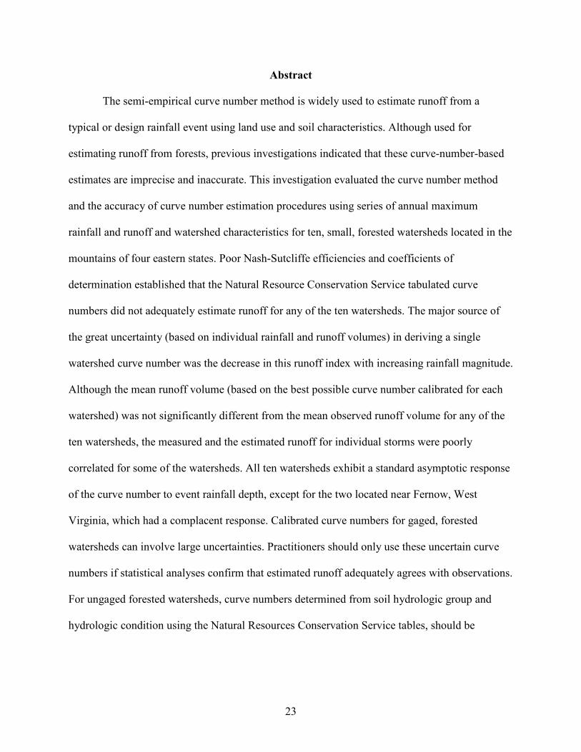
Abstract

The semi-empirical curve number method is widely used to estimate runoff from a

typical or design rainfall event using land use and soil characteristics. Although used for

estimating runoff from forests, previous investigations indicated that these curve-number-based

estimates are imprecise and inaccurate. This investigation evaluated the curve number method

and the accuracy of curve number estimation procedures using series of annual maximum

rainfall and runoff and watershed characteristics for ten, small, forested watersheds located in the

mountains of four eastern states. Poor Nash-Sutcliffe efficiencies and coefficients of

determination established that the Natural Resource Conservation Service tabulated curve

numbers did not adequately estimate runoff for any of the ten watersheds. The major source of

the great uncertainty (based on individual rainfall and runoff volumes) in deriving a single

watershed curve number was the decrease in this runoff index with increasing rainfall magnitude.

Although the mean runoff volume (based on the best possible curve number calibrated for each

watershed) was not significantly different from the mean observed runoff volume for any of the

ten watersheds, the measured and the estimated runoff for individual storms were poorly

correlated for some of the watersheds. All ten watersheds exhibit a standard asymptotic response

of the curve number to event rainfall depth, except for the two located near Fernow, West

Virginia, which had a complacent response. Calibrated curve numbers for gaged, forested

watersheds can involve large uncertainties. Practitioners should only use these uncertain curve

numbers if statistical analyses confirm that estimated runoff adequately agrees with observations.

For ungaged forested watersheds, curve numbers determined from soil hydrologic group and

hydrologic condition using the Natural Resources Conservation Service tables, should be

24

independently confirmed using locally calibrated curve numbers from gaged watersheds with

similar hydrologic conditions

Keywords: Curve number, runoff-rainfall relationship, watershed, forest, runoff modeling,

hydrology, gaged watersheds, ungaged watersheds,

Curve number method

The curve number method is a semi-empirical technique for determining the runoff depth

or volume as a function of land use and treatment, soil hydrologic group, surface condition, and

rainfall depth. The method is widely used because of simplicity, convenience, publication in a

government handbook, and the tradition of extensive ad hoc use. The Soil Conservation Service

introduced the method in 1954, using approximately twenty years of infiltration or rainfall-runoff

observations from small, rural watersheds (NRCS, 2001; McCutcheon et al., 2006). The Soil

Conservation Service developed the method originally for cropland and rangeland to assess

varying land uses and soil characteristics for designing national flood controls (Rallison and

Miller, 1982). The curve number method is therefore useful for agricultural watersheds,

moderately useful for rangelands, and performs poorly for forests (Hawkins, 1993). The method

was extended to urban runoff design (SCS, 1975), now a dominant application.

Use of curve number method

The use of curve numbers has evolved since 1954. Despite the limited scope of intended

applications and identification of several problems (e.g., Ponce and Hawkins, 1996; Jacobs et al.,

2003; McCutcheon et al., 2006), curve numbers are now widely used in environmental fate and

25

transport models worldwide (Woodward et al., 2002). The following types of models are based

on the curve number approach:

• Water balance and storm routing models (Yu et al., 2001; De Michele and

Salvadori, 2002)

• Water quality models (Rode and Lindenschmidt, 2001)

• Coupled meteorological and hydrological models (Yu et al., 1999)

• Crop growth models (Irmak et al., 2001)

Specific examples of models include the

• Chemicals, Runoff, and Erosion From Agricultural Management Systems

(CREAMS; Knisel, 1980)

• Erosion Productivity Impact Calculator (EPIC; Sharpley and Williams, 1990)

• Simulator for Water Resources in Rural Basins (SWRRB; Williams et al., 1985;

Arnold et al., 1990)

• Soil and Water Assessment Tool (SWAT; Arnold et al., 1993)

• Agricultural Non-Point Source Pollution Model (AGNPS; Young et al., 1989)

• Generalized Watershed Loading Functions (GWLF) for stream flow and nutrients

(Haith and Shoemaker, 1987)

The curve number method has a number of limitations, which are not widely recognized

(Ponce and Hawkins, 1996; Jacobs et al., 2003; McCutcheon et al., 2006) and that are rarely

noted in textbooks (e.g., Hammer and MacKichan, 1981; Roberson et al., 1988; Bras, 1990;

Helweg, 1991; Bedient and Huber, 1992). Chief among the limitations is that the method does

not represent runoff rates, paths, and source areas upon which erosion and water quality

simulations depend. In addition, the Natural Resource Conservation Service (and Soil

26

Conservation Service, before) never adapted the method to estimate forest runoff, only runoff

from agricultural lands, rangelands, and urban areas. Furthermore, the accuracy of the curve

number method has not been thoroughly evaluated (McCutcheon et al., 2006) and using the

curve number table (NRCS, 2001) for engineering design may not provide reliable estimates of

runoff (Schneider and McCuen, 2005). Use of the curve number method to estimate runoff

volume from forested watersheds usually results in unacceptable estimates runoff (Ponce and

Hawkins, 1996; McCutcheon, 2003; Jacobs et al., 2003; Garen and Moore, 2005; Michel et al.,

2005; Schneider and McCuen, 2005; McCutcheon et al., 2006).

These poorly recognized and misunderstood limitations evidently have led to a number of

misinterpretations and misapplications. As a result, this study investigated the curve number

method to evaluate the applicability and accuracy for forested watersheds.

Curve number and runoff equation

The curve number method estimates runoff depth or volume, Q, from rainfall depth or

volume, P, based on the conservation of water in a watershed

QFIP a ++= (2.1)

and two hypotheses that can be expressed on a typical or design event basis, as

S

F

IP

Q

a

=−

(2.2)

SIa λ= (2.3)

where Ia is the watershed initial abstraction (includes interception, depression storage, and

infiltration losses prior to ponding and the commencement of overland or quick flow); F is the

typical event retention of water; S is the potential maximum retention of water after the initial

27

abstraction Ia occurs; and λ is the dimensionless initial abstraction ratio or coefficient. Typically

expressed in inches for practice in North America and millimeters in most other parts of the

world, rainfall, runoff, initial abstraction, retention, and potential maximum retention have the

dimensions of volume or depth (volume normalized by watershed area). Equation (2.1) is a

simple continuity relationship introduced to determine a typical event runoff of sufficiently

limited duration so that evapotranspiration is negligible (Yuan et al., 2001). The partitioning of

rainfall into runoff and retention is based on the first hypothesis [Equation (2.2)]. This hypothesis

expressed as the ratio of runoff Q to the effective rainfall (event rainfall excluding initial

abstraction) P - Ia is equal to the ratio of watershed moisture retention F as a result of the rainfall,

to the potential maximum retention S (Ponce and Hawkins, 1996).

The potential maximum retention (S), the maximum amount of water that can be

temporarily stored or retained according to the antecedent conditions on a watershed, is constant

for a particular storm. However, potential maximum retention varies somewhat from storm to

storm because of the variation of soil moisture, mainly due to antecedent rainfall (Yuan et al.,

2001). Nevertheless, the Soil Conservation Service assumed that the potential maximum

retention was constant for each watershed as long as land cover and use, and hydrologic

condition did not change. The retention (F), defined as the difference between typical event

rainfall P and typical event runoff Q, also varies from one storm to a different storm because the

magnitude of storm rainfall varies. The Soil Conservation Service approach specifically ignored

storm rainfall-runoff dynamics including changes in rainfall intensity, event duration, infiltration

rates, and runoff hydrographs. Because retention, F, is assumed to be constant for a given rainfall

volume despite varying rainfall intensities and durations and potential maximum retention S

constant for a watershed, the method was not intended to accurately estimate runoff for specific

28

rainfall events. The curve-number-based estimate of runoff is only the typical or average

response to a given rainfall volume (Ponce, 1996). However, the Natural Resource Conservation

Service (2001) handbook encouraged curve number use in developing a rainfall excess interval

for unit hydrographs.

The relation between initial abstraction, Ia , and potential maximum retention, S, has not

been fundamentally defined. The original circa 1954 linear relationship [Equation (2.3)] is

necessary to avoid an independent estimation of initial abstraction, Ia. Equation (2.3) was

justified based on daily measurements of rainfall and runoff on watersheds of fewer than four

hectares (ten acres), but half of the initial abstractions derived from daily observations were

between 0.095 and 0.38 (NRCS, 2001). Despite the large uncertainty, a standard value for the

initial abstraction ratio, λ = 0.2, was adopted by the Soil Conservation Service. Later studies in

the United States and other countries documented initial abstraction ratios varying between 0.00

< λ < 0.38 (Ponce and Hawkins, 1996). Victor Mockus, a pioneer of the curve number method

(Ponce, 1996), agreed with changing the original ratio of λ = 0.2 to 0.1 or 0.3, or any other value,

if the data under consideration warranted. Most troubling, Mockus said that the method was

developed for storm events, but the determination of λ = 0.2 was based on daily measurements of

rainfall and runoff because these were the only data available for the analyses.

As the method is currently practiced, typical event runoff, Q, can be computed with the

curve number based on the land use and cover, hydrologic soil group and condition, and the

rainfall depth by combining Equations (2.1) and (2.2) as

( )SIP

IPQ

a

a

+−−

=2

(2.4)

29

Equation (2.4) is valid for P > Ia and Q = 0 otherwise; no runoff occurs when the rainfall depth is

less than or equal to the initial abstraction, Ia. With initial abstraction included in Equation (2.4),

the actual retention, F = P – Q, asymptotically approaches a constant, S + Ia, as storm event total

rainfall increases.

For λ = 0.2, Equation (2.4) becomes

Q =P − 0.2S( )2

P + 0.8S( ) for P > 0.2S

Q = 0 for P ≤ 0.2S (2.5)

Besides rainfall, P, that is monitored widely in the United States and other countries, Equation

(2.5) contains only one other parameter (potential maximum retention S, which varies between 0

and ∞). For convenience in practical applications, potential maximum retention, S, was defined

in terms of a dimensionless parameter, CN (curve number), which was designed to vary in a

more restricted range of 100 ≥ CN ≥ 0 as follows:

101000

−=CN

S ⇒ 10

1000

+=S

CN (S in inches) (2.6a)

or

254400,25

−=CN

S ⇒254

400,25

+=S

CN (S in millimeters) (2.6b)

The Soil Conservation Service selected 1000 and 10 (in inches) as expressed in Equation (2.6a)

or 25,400 and 254 (in millimeters) in Equation (2.6b) to have the same units as potential

maximum retention, S. Zero potential maximum retention (S = 0 or CN = 100) represents an

impermeable watershed; CN = 0 represents a mathematical upper bound to the potential

maximum retention (S = ∞), which is an infinitely abstracting watershed. According to current

30

practice, specification of an event rainfall depth and the watershed curve number CN should

allow an estimate of watershed runoff using Equations (2.5) and (2.6).

Watershed curve numbers are estimated based on land use, hydrologic condition, and

hydrologic soil group for ungaged watersheds from standard tables (NRCS, 2001) or calculated

by algebraic rearrangement of Equations (2.5) and (2.6) for gaged watersheds as

( ) 105425

1000

21

2 +

+−+

=PQQQP

CN (2.7a)

or

( ) 2545425

400,25

21

2 +

+−+

=PQQQP

CN (2.7b)

Measured pairs of rainfall volume, P, and runoff volume, Q, are used in Equation (2.7) to

determine the curve number CN. The pairs of P and Q are the measured rainfall and direct runoff

from a storm event in inches or millimeters for Equations (2.7a) and (2.7b), respectively.

Study watersheds

Ten small, forested watersheds in the mountains of four eastern states (Figure 2.1)

provided rainfall-runoff measurements, and were located in the Etowah River basin (Georgia),

Coweeta Hydrologic Laboratory (North Carolina), Fernow Experimental Forest (West Virginia),

and Hubbard Brook Experimental Forest (New Hampshire). Long-term records of rainfall and

runoff were available except for the watersheds, Etowah 2 and 3 (Table 2.1). The study includes

four watersheds from the Coweeta Hydrologic Laboratory (Coweeta 2, 28, 36, and 37), and two

watersheds each from the Fernow Experimental Forest (Fernow 3 and 4) and Hubbard Brook

Experimental Forest (Hubbard Brook 3 and 5). The size of watersheds ranges from 12.26 to

31

144.1 hectares (30.29 to 356.1 acres) and elevation ranges from 488 to 1,591.4 meters (1,601 to

5,221 feet).

The Etowah River basin is located in the Blue Ridge Physiographic Province of the north

Georgia. This study complied information from two from total of thirteen forested watersheds

from the northern portion of the Etowah basin within the Chattahoochee National Forest.

Elevation ranges between 451 and 710 meters (1,480 feet to 2,329 feet) and average slope varies

from 10.1 to 12.6 percent. Etowah 2 and 3 soils are fine loam, sandy loam, and sandy.

The Coweeta Hydrological Laboratory is located in the Blue Ridge Physiographic

Province of the southern Appalachian Mountains, near Otto, NC. The Laboratory elevation

ranges from 675 to 1,592 meters (2,215 to 5,223 feet) and average slope ranges between 60.2 to

70.6 percent. The Coweeta soil depth averages approximately 7 m (23 ft) in depth at low to mid

elevations (Coweeta 2) and is much more shallower (<2 m, 6.6 ft) at high elevations (Coweeta

36) (McCutcheon et al., 2006). Of the 17 instrumented watersheds at Coweeta, this study

evaluated four. These four encompassed the range in elevation, vegetation, soil depth, rainfall,

and other climatic factors and hence in hydrologic response found in the Coweeta Hydrological

Laboratory. The soils are inceptisols and ultisols (Typic Hapludults and Humic Hapludults). The

forest cover included northern hardwoods, cove hardwoods, xeric oak and pine, oak and hickory,

and mixed oak (USDA, 2004).

The Fernow Experimental Forest lies in the Allegheny Mountain section of the

unglaciated Allegheny Plateau and had ten experimental watersheds. Fernow elevations range

from 533 to 1,113 meters (1,749 to 3,652 feet) with generally steep slopes. Almost all Fernow

soils (including the sandstone, shale, and limestone soils) are well-drained, medium textured

loams and silt loams characterized by stoniness. Average soil depth to bedrock ranged for the

32

most part from 91 centimeters to 152 centimeters (36 inches to 60 inches) and humus depth

averaged approximately 6 centimeters (2 inches). The forest cover included northern red oak,

chestnut oak, white oak, scarlet oak, black oak, and upland oak (Reinhart et al., 1963).

The Hubbard Brook Experimental Watershed was located in the White Mountain

National Forest. The bowl-shaped Hubbard Brook Valley has hilly terrain, ranging in elevation

from 222 to 1,015 meters (728 to 3,330 feet). The Experimental Forest had seven instrumented

watersheds, two of which were used in this investigation. Soils are predominantly well-drained

spodosols derived from glacial till with a sandy loam texture. Average soil depth, including

unweathered till, was approximately 2 meters (6 feet) from surface to bedrock, although this was

highly variable. Average humus depth of Hubbard Brook is 6.9 centimeters (2.7 inches). The

second-growth forest is even-aged and consists of 80 percent to 90 percent northern hardwoods

and 10 to 20percent spruce (USDA, 2004).

Determination and testing of curve numbers

Five procedures were used to determine gaged watershed curve numbers from rainfall-

runoff series, including the: (1) arithmetic mean (Bonta 1997), (2) median (NRCS, 2001), (3)

geometric mean (NRCS, 2001), (4) standard asymptotic fit (Sneller, 1985; Hawkins, 1993), and

(5) nonlinear least squares fit (Hawkins, 1993). This investigation compared these five curve

numbers calibrated to gaged watersheds with the tabulated curve number based on the

corresponding forested watershed hydrologic soil class and condition (NRCS, 2001). Table 2.2

summarizes these methods and the Appendix provides additional information about how these

procedures were used to determine curve numbers.

33

This study used annual series of maximum rainfall and of maximum runoff volume for

the record available for each watershed (NRCS, 2001) located at Coweeta, Fernow, and Hubbard

Brook. The maximum peak flow of the year and the associated rainfall was the basis of the

annual series for Fernow and Hubbard Brook. The maximum runoff volume of each year of the

record at Coweeta was the basis of these annual series. The Etowah 2 and 3 watersheds,

however, had only 21 months of measured rainfall-runoff and, hence, all storms with 25

millimeters (one inch) or more of total rainfall volume and the corresponding measured runoff

volume are used for partial duration series. Etowah events with rainfall of fewer than 25

millimeters (one inch) produced minimal runoff and thus were not useful for this evaluation.

The five methods to determine a watershed curve number and the Natural Resources

Conservation Service (2001) tabulation produced six estimates for each watershed. This study

used the six curve numbers and the rainfall series for each watershed to generate series of

estimated runoff for comparison with the corresponding series observed runoff of an equal

number. The investigation estimated watershed runoff, Q, using Equations (5) and (7). The

investigation assessed the relative accuracy of the six procedures for calculating runoff from the

rainfall depth in comparison to measured runoff using the coefficient of efficiency or Nash-

Sutcliffe efficiency (Nash and Sutcliffe, 1970)

( )

( )∑

∑

=

=

−

−−=

n

i

ooi

n

i

cioi

NS

QQ

QQ

E

1

2

1

2

1 (2.8)

and the coefficient of determination

( )

( )∑

∑

=

=

−

−−=

n

i

ooi

n

i

eici

QQ

QQ

D

1

2

1

2

1 (2.9)

34

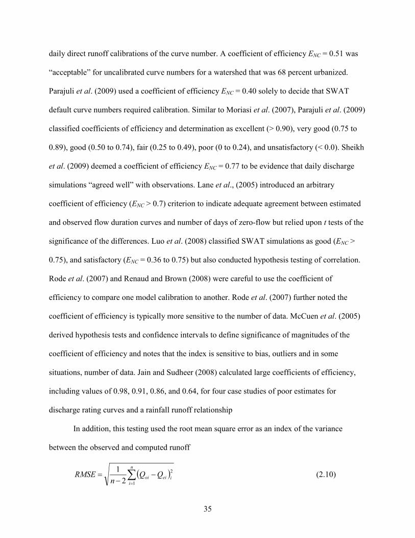
where n is the total number of rainfall-runoff events in the period of record (Table 2.1), i is the

number of each event from 1 to n, Qoi is the observed storm runoff, Qci is the computed runoff,

oQ is the mean of the observed runoff, and Qei the estimated runoff obtained from the regression

of Qoi and Qci.

The coefficient of efficiency, ENC, describes the degree of association between the

observed and measured runoff, as does the coefficient of determination. Although a good

measure of the association between the observed and the calculated runoff, the coefficient of

determination does not reveal systematic error (Aitkin, 1973). If the observed and estimated

runoff are highly correlated but biased (not randomly deviating from the perfect correlation of

observed versus estimated runoff), the coefficient of efficiency, ENS, is smaller than the

coefficient of determination D (Aitkin, 1973). Both the coefficient of determination, D, and the

coefficient of efficiency, ENS, is always less than unity and large values may indicate accurate

estimates of runoff volume (Hope and Schulze, 1981; McCuen et al., 2005; Jain and Sudheer,

2008). The coefficient of efficiency for unbiased estimates, based on linear relationships, range

between 0 to 1, corresponding to no or minimal correlation to perfect correlation, respectively.

Yet, linear relationships are rare in hydrology. A negative coefficient of efficiency, ENS, can

occur for biased estimates and establishes that the mean of the series of all observed maximum

annual runoff for a watershed is a better estimate than the runoff calculated with the runoff

equation based on the curve number.

Santhi et al. (2001) used an arbitrary criterion of coefficient of efficiency ENC > 0.5 to

evaluate monthly runoff estimates using the Soil Water Assessment Tool (SWAT), based on the

curve number method. Lim et al. (2006) the coefficient of efficiency ENC = 0.67 “acceptable” for

simulations of annual runoff using the curve number method but used criteria of 0.5 and 0.6 for

35

daily direct runoff calibrations of the curve number. A coefficient of efficiency ENC = 0.51 was

“acceptable” for uncalibrated curve numbers for a watershed that was 68 percent urbanized.

Parajuli et al. (2009) used a coefficient of efficiency ENC = 0.40 solely to decide that SWAT

default curve numbers required calibration. Similar to Moriasi et al. (2007), Parajuli et al. (2009)

classified coefficients of efficiency and determination as excellent (> 0.90), very good (0.75 to

0.89), good (0.50 to 0.74), fair (0.25 to 0.49), poor (0 to 0.24), and unsatisfactory (< 0.0). Sheikh

et al. (2009) deemed a coefficient of efficiency ENC = 0.77 to be evidence that daily discharge

simulations “agreed well” with observations. Lane et al., (2005) introduced an arbitrary

coefficient of efficiency (ENC > 0.7) criterion to indicate adequate agreement between estimated

and observed flow duration curves and number of days of zero-flow but relied upon t tests of the

significance of the differences. Luo et al. (2008) classified SWAT simulations as good (ENC >

0.75), and satisfactory (ENC = 0.36 to 0.75) but also conducted hypothesis testing of correlation.

Rode et al. (2007) and Renaud and Brown (2008) were careful to use the coefficient of

efficiency to compare one model calibration to another. Rode et al. (2007) further noted the

coefficient of efficiency is typically more sensitive to the number of data. McCuen et al. (2005)

derived hypothesis tests and confidence intervals to define significance of magnitudes of the

coefficient of efficiency and notes that the index is sensitive to bias, outliers and in some

situations, number of data. Jain and Sudheer (2008) calculated large coefficients of efficiency,

including values of 0.98, 0.91, 0.86, and 0.64, for four case studies of poor estimates for

discharge rating curves and a rainfall runoff relationship

In addition, this testing used the root mean square error as an index of the variance

between the observed and computed runoff

( )∑=

−−

=n

iieioi QQ

nRMSE

1

2

2

1 (2.10)

36

This statistical testing also compared estimated runoff to measured runoff using the two-tailed

paired Student t-test at the 0.05 significance level. The null and alternative hypotheses

determined if the differences in the estimated and the corresponding measured runoff were

significantly different from zero. Finally, Duncan multiple comparison tests determined

significant differences between the six estimated runoff volumes and the corresponding

observations.

Results of testing curve numbers

Table 2.2 presents the variations of curve numbers for each watershed derived by the five

approaches plus the appropriate curve numbers tabulated by the National Resources

Conservation Service (2001) for ungaged drainages. Table 2.2 also reports the appropriate

measure of the uncertainty for each of the different curve numbers calculated by the six

approaches evaluated by study. The magnitude of the range, the appropriate measure of

uncertainty for the median, varied from 27 (Fernow 4) to 48.5 (Coweta 37) and for the geometric

mean, the 95 percent confidence interval varied from 19.6 (Coweeta 37) to 55.9 (Coweeta 36).

The magnitude for the 95 percent confidence interval for the arithmetic means varied from 23.4

(Coweeta 28) to 50.4 (Coweeta 2).

Figure 2.2 strongly indicates that most of the large uncertainty in determining a single

calibrated curve number for a watershed is due to variation with event rainfall magnitudes. As

the event, rainfall volume increases the curve number decreases for all ten watersheds (four not

shown).

From Table 2.2, 80 percent of the geometric mean curve numbers for the ten watersheds

were greater than curve numbers based on the other estimation procedures. For the exceptions,

37

Etowah 2 and Hubbard Brook 5, the median yielded the largest calibrated curve number. For 40

percent of the watersheds (Table 2.2), the arithmetic mean occurred between the similar-in-

magnitude, geometric mean and median. The curve numbers based on the nonlinear least squares

fit and the asymptote of the standard watershed response were always smaller than the median,

geometric mean, and arithmetic mean curve numbers.

Table 2.3 records the statistics used to test the applicability and accuracy of the curve

number method to estimate runoff from tabulated curve numbers for ungaged watersheds and

from the five approaches to determine calibrated curve numbers for gaged watersheds. Figure 2.3

presents observed runoff Qo versus estimated runoff Qe to illustrate the deviation from the perfect

correlation Qo = Qe for the “best” curve numbers calibrated. Figure 2.4 better illustrated the bias

in runoff estimates based on the “best” curve numbers.

The accuracy of curve numbers (Table 2.3) in estimating runoff comparable to the

observed runoff was investigated using the Nash-Sutcliffe efficiency ENS [Equation (2.9)] and the

coefficient of determination D [Equation (2.8)]. For Etowah 2, Hubbard Brook 3, and Hubbard

Brook 5, a simple average for each one of the observed runoff series was a better estimate of the

runoff than estimates using the tabulated curve numbers (due to the negative Nash-Sutcliffe

efficiencies in Table 2.3). For 60 percent of the watersheds (Coweeta 36, Coweeta 37, Fernow 3,

Fernow 4, Hubbard Brook 3, and Hubbard Brook 5), differences in the Nash-Sutcliffe efficiency

and coefficient of determination (Table 2.3) established runoff bias as indicated in Table 2.2 and

Figure 2.4.

For each watershed listed in Table 2.3, the root mean square error was greatest for the

curve number estimate that was the greatest or smallest. Nevertheless, this measure of bias varied

little between the six approaches to select a curve number for any given watershed. Coweeta 37

38

(third shortest period of record or third fewest degrees of freedom) consistently had the largest

root mean square error for all six approaches; Etowah 3 (next to the smallest degrees of

freedom), consistently the smallest.

In Table 2.3, neither the coefficients of efficiency nor determination indicated that runoff

based on the five methods of calibration and the asymptotic curve number was highly correlated

with observations. The limited correlation may be consistent with the large uncertainty recorded

in Table 2.2 and Figures 2.3 and 2.4. For Coweeta 36, Coweeta 37, and Hubbard Brook 3, little

bias was evident from the similar magnitude of the Nash-Sutcliffe efficiency and the coefficient

of determination. Based on the differences between the coefficients of efficiency and

determination, five of ten runoff estimates based on the asymptotic curve number indicated bias;

30 percent based on the nonlinear least squares; and 10 percent based on the arithmetic mean

curve number. Nevertheless, none of the indications of bias was as severe as the biases of the

tabulated curve numbers for Coweeta 36, Coweeta 37, Fernow 3, Fernow 4, Hubbard Brook 4,

and Hubbard Brook 5. Figure 2.4 for the “best” curve numbers indicated some bias for almost all

of the watersheds. This results provides evidence for the bias in all the observed versus estimated

runoff and is due to lack of an explicit means for soil moisture accounting.

Table 2.4 listed the best curve numbers calibrated for each of the ten watersheds with one

of five methods tested. The paired Student t-test established that none of the estimated runoff

based on the best curve number differed from observed with a 0.05 chance of error.

The Duncan multiple comparison tests in Table 2.5 established that the estimated runoff

based on the tabulated curve number (TQ) was significantly different from the observed runoff

from Coweeta 36, Coweeta 37, Fernow 3, Fernow 4, Hubbard Brook 3, and Hubbard Brook 5.

Using the means in Table 2.5, the runoff estimates based on the geometric mean curve number

39

was ranked first or second for all ten watersheds. The median ranked first for Etowah 2 and

Hubbard Brook 5. Regardless of the rankings, the multiple comparison tests (Table 2.5) revealed

no significant difference (at the 0.05 percent level of significance) in using the median,

geometric mean, and arithmetic mean curve numbers to estimate runoff for all ten watersheds.

Sneller (1985) suggested an arbitrary, unproven criterion to determine whether the

standard asymptotic fit to watershed curve numbers was adequate [Equation (A-9); the measured

range of rainfall covers 90 percent of the slopes of the rainfall-curve number watershed

response]. Table 2.6 showed that the rainfall records should be suitable to determine standard

asymptotic curve numbers according to Sneller (1985), except for Fernow 3 and Fernow 4,

because the maximum rainfalls recorded for each watershed were greater than 58.496/k

millimeters or 2.303/k inches for the length of record used in this study. The constants k and the

asymptotic curve number arose from fitting the empirical curve number-rainfall relationship to

the observed event rainfalls and estimated curve numbers [see Equations (A-6) to (A-14)].

Accuracy and applicability of curve numbers

For Etowah 2 and the Hubbard Brook watersheds, the estimated runoff based on the

tabulated curve numbers (NRCS, 2001) was so poor that the average of the series of observed

runoff for these drainages provided better estimates. Runoff estimated for the tabulated curve

numbers for six of the ten watersheds was significantly smaller than the observed as noted in

Table 2.5. Only the tabulated curve numbers for Coweeta 2, Coweeta 28, and Etowah 3 provided

adequate runoff estimates. Seventy percent of the tabulated curve numbers resulted in less

estimated runoff compared to the extensive observations of up to 68 years of record. The smaller

Nash-Sutcliffe efficiencies compared to the coefficient of determination for the higher elevation

40

Coweeta 36 and Coweeta 37, Fernow, and Hubbard Brook and Figure 2.3, establish that

estimated runoff only marginally correlates to observed runoff and may be biased (Aitkin, 1973;

McCuen et al., 2005).

The reason for the biased tabulated curve numbers for the National Resources

Conservation Service (2001) land use category “woods” is difficult to determine. The original

watershed rainfall-runoff measurements used in circa 1954 to estimate the tabulated curves for

“woods” is missing (Hawkins, 2006) and this investigation could not confirm the accuracy of the

table or the degree of uncertainty associated with each entry. The only possible sources of error

to contemplate were the assigned soil hydrologic group and the selected hydrologic condition of

good.

One source of early concern for the field of hydrology in using the curve number method

was that many soils may be misclassified, especially those in the Groups B and C (Neilsen and

Hjelmfelt, 1998). Nevertheless, the likelihood of misclassification at these national experimental

forests is limited and cannot explain all of these large discrepancies in curve numbers. If the

higher elevation Coweeta 36 and 37 soils were hypothetically in Group C, not B for example, the

curve number 70 for woods would better agree with curve numbers determined from rainfall-

runoff measurements. As recently as 2005, a U.S. Department of Agriculture soil scientist

reexamined the Fernow soils and changed the hydrologic group from B to C, a curve number

change from 55 to 70. However, even a change to Group D (77) would not match curve number

calibrations for the Fernow and Hubbard Brook rainfall-runoff observations. Moreover, Group D

is definitely not consistent with the National Engineering Handbook (NRCS, 2001) guidance,

especially for steep mountain forests where high water tables and waterlogged soils are rare

outside of a few landslide-prone areas.

41

Several independent personal observations of the good hydrologic conditions maintained

and expected in national forests and experimental forests puts this specification beyond doubt for

the curve number procedure as written (NRCS, 2001). As a result, neither selection of soil

hydrologic group nor hydrologic condition explained all of the severe bias of the woods land-use

category in consistently underestimating runoff. If the curve number method consistently

underestimated runoff from undeveloped forest, the effect of urbanization will be consistently

overestimated and drainage controls overestimated, perhaps to explain part of the annual

overdesign costs estimated to be as great as $2 billion per year (Schneider and McCuen, 2005).

Because the tabulated curve numbers were unreliable, the next important question was,

can an engineer or hydrologist calibrate the watershed curve number from gage data and

extrapolate to a similar ungaged watershed? Prior to addressing this issue, this investigation

examined the procedures to derive a watershed curve number from series of rainfall-runoff

observations (for which standardization is lacking).

The calculation of watershed curve numbers from rainfall-runoff measurements had

precedent but lacked justification and rationale. The Natural Resources Conservation Service

(2001) based the tabulated curve numbers on the median—easily determined graphically from

rainfall P versus runoff Q. Later citing Yuan (1933) as the only proof, the Natural Resources

Conservation Service (2001) designated the geometric mean as the appropriate way to express

the watershed curve number and calculate 95 percent confidence intervals. The geometric mean

closely approximates the median if the distribution of curve numbers determined for a watershed

is lognormal (Yuan, 1933) but proof of this curve number lognormality did not appear in the

literature. Nevertheless, Tables 2.2, 2.3, and 2.5 indicated that the distribution was approximately

lognormal for these ten mountainous watersheds because the runoff estimated from the median

42

and geometric mean curve numbers was not significantly different. However, because the

arithmetic mean curve number falls between the median and geometric mean for 40 percent of

the watersheds, statistical proof of the lognormal distribution as the best fit may not be possible

for these observations. Bonta (1997) seemed to be the first to calculate the arithmetic mean curve

number but also did not justify this choice with proof that the curve number distributions were

normal.

Unlike the means and median, some of the nonlinear least squares fit and asymptotic

curve numbers produced significantly different runoff estimates as noted in Table 2.5. Forty

percent of the watersheds had runoff estimated based on the asymptotic curve number

significantly different from observations. The asymptotic curve numbers for the Etowah

watersheds estimated unsatisfactory runoff due to negative coefficients of efficiency. Using the

nonlinear-least-squares-fit curve number, Etowah 2 had the only unsatisfactory estimated runoff.

Coweeta 2 was a watershed for which none of the calibrated curve numbers produced

runoff estimates significantly different from the observed. Yet the runoff estimated using the

nonlinear least squares fit and asymptotic curve numbers was significantly different from that

estimated using the means and median.

The asymptotic curve number based runoff was significantly different from the estimated

runoff based on geometric mean curve number for Coweeta 36 but not significantly different

from the observed runoff. For Fernow, estimated runoff from both watersheds was significantly

different from that estimated with the asymptotic curve versus the estimated with means and

median and versus the measured. Also for Fernow, the estimated runoff based on the nonlinear-

least-squares-fit curve number was significantly different from that based on the geometric mean

but not the observed. For Etowah 2, Etowah 3, Coweeta 28, Coweeta 37, Hubbard Brook 3, and

43

Hubbard Brook 5, the t-test did not resolve any differences in runoff estimates and the observed,

which indicated some lack of robustness in the t-test. That estimated runoff based on the

asymptotic curve number was not significantly different for all ten watersheds seemed to be a

reflection of the high degree of variance of event curve numbers (Tables 2.2 and 2.4) from the

single watershed curve number based on central tendencies, minimization of least squares, and

the asymptotic limit. The nonlinear-least-squares-fit curve number was always smaller that the

watershed curve numbers derived from central tendencies on all ten watersheds, but these four

methods to calibrate the curve number never produce runoff that was significantly different from

the observed. (However, Etowah 2 runoff estimates were unsatisfactory based on the nonlinear

least squares fit.) Therefore, the Duncan multiple comparison tests did not distinguish any

advantage to choosing the median, geometric mean, arithmetic mean, or nonlinear-least-squares-

fit curve numbers; all are equally capable of estimating runoff to at least within a five percent

chance of error for these small mountainous-forested watersheds. Nevertheless, coefficient of

efficiency for Etowah 2 indicated some lack of robustness in the t-tests.

Using the Nash-Sutcliffe efficiency in Table 2.4 to rank these equally valid methods, the

median ranked best for 70 percent of the watersheds. Nevertheless, any of the other three

methods provided better estimates of the great uncertainty (as 95-percent confidence intervals

versus the range of curve numbers) in single-value watershed curve numbers.

Even after the adoption of the method for urban hydrology (SCS, 1975) and use with

well-defined design rainfalls (e.g., 10-year and 100-year rainfall return intervals), the

inconsistency with using curve numbers based on return intervals of two years were not

explicitly noted until recently (McCutcheon et al., 2006). (The median, geometric mean, and

arithmetic mean curve numbers by definition have a return interval of two years or a probability

44

of occurrence of 50 percent if now skew is present.) Further, after Sneller (1985) and Hawkins

(1993) noted that watershed curve numbers are typically a function of storm event rainfall

volume (Figure 2.2), the implied assumption of lognormality and adequacy of the median or

geometric mean curve numbers have never been examined. The probabilistic approaches of

Hjelmfelt (1980), Pilgrim and Cordery (1993), and Titmarsh et al. (1995) seem to recognize that

watershed curve numbers varied as return intervals before McCutcheon et al. (2006) noted the

need to calibrate curve numbers for specific design return intervals. Because each measured

rainfall volume has a frequency of occurrence, McCutcheon et al. (2006) could relate a return

interval to a variable watershed curve number as Titmarsh et al. (1995) and Pilgrim and Cordery

(1993) accomplished differently earlier.

The finding that all ten mountainous-forested watershed curve numbers varied with event

rainfall explained several issues involving the curve number method. Firstly, the standard (or

perhaps complacent for Fernow) responses clearly explains in Table 2.2 why the asymptotic

curve numbers associated with infinitely or very large rainfall was always less than the geometric

mean, arithmetic mean, and median associated with a two-year return interval. Secondly, the

variability with event rainfall explained much but not all of the large uncertainty in calibrated

curve numbers. Finally, this large variability for forested watersheds with event rainfall

explained why a single watershed curve number was difficult to select. As Titmarsh et al. (1995)

and McCutcheon et al. (2006) noted, many watersheds seem to require a variable curve number

that is different for different design intervals, not the single watershed curve number that Mockus

and the Soil Conservation originally conceived (Ponce, 1996; NRCS, 2001).

The wide differences in magnitudes of ranges and 95-percent confidence intervals

indicated that the response of a watershed depends on the range of maximum annual rainfall,

45

antecedent moisture, rainfall intensity, and type of seasons (dormant or growing). Variable

source areas responsible for runoff generation vary in size depending on the magnitude of

rainfall, which results the amount of rainfall influence the values of curve number. For all

watersheds, the curve number values decrease as the magnitude of rainfall increase (Figure 2.2).

In addition, the curve number method lacks a method that considers initial moisture content of

the soil because the preexisting condition affects the rate of runoff generation.

This investigation could not distinguish between any of the methods of calibrating a

singular watershed curve number from rainfall-runoff measurements and a central-tendency-

based curve number. The exception was that the asymptotic curve number produced

unsatisfactory or different estimates of runoff than observed for 60 percent of the watersheds.

One estimate based on the nonlinear least squares fit was unsatisfactory, but this was for Etowah

2 for which only 21 months of observations were available and variability of rainfall events

greater than 25 millimeters (1 inch) may have been different than the variability for the other

series of annual maximum runoff. Although this investigation could not rule out use of calibrated

curve numbers with a 2-year return interval for a singular watershed curve number mountainous

forests, these can only be resorted to when a practitioner expects limited curve number

variability. For high variability in mountainous-forested watershed curve numbers the

practitioner should estimated the curve numbers for the asymptotic limit (infinite return interval)

and 10-year, 100-year, and other design return intervals.

Limited uses and additional investigation necessary

Although the curve number method was widely used for estimating runoff depths or

volumes, practitioners may have only poorly understood the limitations and uncertainties,

46

especially for ungaged forested watersheds of the mountainous eastern United States. The

Natural Resource Conservation Service (2001) tabulated curve numbers based on ungaged

watershed characteristics were not adequate to estimate runoff from ten small forested

watersheds in the mountainous eastern United States. Most of the runoff estimated from the

tabulated curve numbers was unreliable. Even the misclassification of the soil hydrologic group

was not adequate to explain the significant bias in runoff estimates. Therefore, practitioners

should not use the current Natural Resource Conservation Service (2001) tabulations for

“woods” to estimate runoff for designs and careful policy analysis involving forested watersheds.

At best, engineers and hydrologist must confirm estimated runoff from mountainous-forested

eastern watersheds with independent runoff estimates if the practitioner cannot calibrate curve

numbers with rainfall-runoff measurements collected from very similar watersheds prior to use

in design calculations or for policy deliberations.

For models that use the curve number as a lumped parameter, the same effective

guidance holds. Model applications should only use tabulated curves as initial values in a careful

calibration procedure. Applications used in policy determinations and design should carefully

evaluate calibrations and model tests for goodness of fit and bias (McCuen et al., 2005).

Of the five calibration procedures, only the asymptotic curve number was unreliable as a

singular estimate of a mountainous-forested watershed curve number. Additional investigation is

necessary to confirm fully the use of the nonlinear least squares fit. The Duncan multiple

comparison tests were not sufficiently robust to distinguish between calibrated curve numbers

based on the median, geometric mean, or arithmetic mean for mountain-forested watersheds.

Therefore, the geometric mean with the 95-percent confidence interval recommended by the

Natural Resource Conservation Service (2001) seems best to provide an estimate of the

47

uncertainty involved with each calibration. The 95-percent confidence interval or a similar

expression of uncertainty is necessary to support a decision on whether use to the 2-year curve

number as a crude approximation of a singular watershed curve number for a continuum of

design return intervals. For large uncertainties of +1or greater, calibrated curve numbers should

be matched to the design return intervals of interest by taking the variability of curve numbers

with event rainfall into account.

The likelihood of simply updating the Natural Resource Conservation Service (1998,

2001) table of curve numbers seems remote despite a call by Schneider and McCuen (2005). The

original information on which the Soil Conservation Service based the table has been lost for the

most part and the original concept that a single lumped index for each watershed largely refuted

(Hawkins, 1993). In addition, the current tabulation is very specific to original assumption that

the initial abstraction was twenty percent of the potential maximum retention. More productive

would seem to be a derivation of a new simplified method to correct the residual effect of the

curve number varying with the state variable, event rainfall. A new derivation could be tailored

to modern web-based computing and advances in remote sensing including uses of digital

elevation models and geographic information systems.

Acknowledgments

Financial assistance provided in part by (1) the West Virginia Division of Forestry, (2)

the U.S. Geological Survey through the Georgia Water Resources Institute, and (3) Warnell

School of Forest and Natural Resources. Richard Hawkins of the University of Arizona, Tucson

provided insightful background and guidance on the use, interpretation, and limitations of the

curve number method. The watershed characteristics and rainfall-runoff series required for this

48

study were provided by Wayne Swank and Stephanie Laseter from the U.S. Forest Service

Coweeta Hydrologic Laboratory; Frederica Wood, from the U.S. Forest Service Fernow Timber

and Watershed Laboratory; John Campbell, from the U.S. Forest Service Hubbard Brook

Experimental Forest; and Josh Romeis from the University of Georgia Etowah Research Project.

References

Aitkin, A. S., 1973. Assessing systematic errors in rainfall-runoff models, Journal of Hydrology

(20): 121-136.

Arnold, J. G, P. M. Allen, and G. Bernhardt, 1993. A comprehensive surface–groundwater flow

model, Journal of Hydrology 142: 47-69.

Arnold, J. G., J. R. Williams, R. H. Griggs, and N. B. Sammons, 1990. SWRRB–A basin scale

simulation model for soil and water resources management. Texas A&M Press, College

Station, Texas.

Bedient, P. B. and W. C. Huber, 1992. Hydrology and Floodplain Analysis. Addison and

Wesley, New York.

Bonta, J. V. 1997. Determination of watershed curve number using derived distributions. Journal

of Irrigation and Drainage Division, American Society Civil Engineers 123(1): 28-36.

Bras, R. L., 1990. Hydrology: An Introduction to Hydrologic Science. Addison and Wesley, New

York.

De Michele, C. and G. Salvadori, 2002. On the derived flood frequency distribution: Analytical

formulation and the influence of antecedent soil moisture condition. Journal of Hydrology

262(1-4): 245-258.

49

Garen, D. C. and D. S. Moore, 2005. Curve number hydrology in water quality modeling: uses,

abuses, and future directions. Journal of the American Water Resources Association 41(2):

377-388.

Haith, D. A. and L. L. Shoemaker. 1987. Generalized watershed loading functions for stream-

flow nutrients. Water Resources Research 23(3): 471–478.

Hammer, M. J. and K. A. MacKichan, 1981. Hydrology and Quality of Water Resources. Wiley,

New York.

Hawkins, R. H., 1993. Asymptotic determination of runoff curve numbers from data. Journal of

Irrigation and Drainage Engineering 119(2): 334-345.

Hawkins, R. H., University of Arizona, Tucson, Personal communication, 2006.

Hjelmfelt, A. T. 1980. Empirical investigation of curve number techniques. Journal of

Hydraulics Engineering Division, 106(HY9): 1471-1476.

Helweg, O. J., 1991. Microcomputers Applications in Water Resources. Prentice Hall,

Englewood Cliffs, New Jersey.

Hope, A. S. and R. E. Schulze, 1981. Improved estimates of stormflow volume using the SCS

curve number method, in Rainfall-runoff Relationship. V. P. Singh, ed., Resources

Publications, Littleton, Colorado, pp. 419-428.

Irmak, A., J. W. Jones, W. D. Batchelor, and J. O. Paz. 2001. Estimating spatially variable soil

properties for application of crop models in precision farming. Transactions of the

American Society of Agricultural Engineers 44(5): 1343-1353.

Knisel, W. G., 1980. CREAMS: A field scale model for chemicals, runoff and erosion from

agricultural management systems. Conservation Research Report No. 26, U.S.. Department

of Agriculture, Southeast Area, Washington, D.C.

50

Lane, P. N. J., A. E. Best, K. Hickel, and L. Zhang. 2005. The response of flow duration curves

to afforestation. Journal of Hydrology 310(1-4): 253-265.

McCutcheon, S.C. 2003. Hydrologic evaluation of the curve number method for forest

management in West Virginia, Report prepared for the West Virginia Division of Forestry,

Charleston, West Virginia.

McCutcheon, S.C., Tedela N.H., Adams, M.B., Swank, W., Campbell, J.L., Hawkins, R.H., Dye,

C.R., 2006. Rainfall-runoff relationships for selected eastern U.S. forested mountain

watersheds: Testing of the curve number method for flood analysis, Report prepared for the

West Virginia Division of Forestry, Charleston, West Virginia.

Michel, C., V. Andre´assian, and C. Perrin. 2005. Soil Conservation Service curve number

method: How to mend a wrong soil moisture accounting procedure? Water Resources

Research 41: W02011, doi:10.1029/2004WR003191.

Nash, J. E. and J. V. Sutcliffe. 1970. River flow forecasting through conceptual models part I-A.

discussion of principles. Journal of Hydrology 10(3): 282-290.

National Resources Conservation Service (NRCS). 2001. Section-4 Hydrology, in National

Engineering Handbook, U.S. Department of Agriculture, Washington, DC.

——1998. Urban hydrology for small watersheds, version 2.1. Technical Release-55, U.S.

Department of Agriculture, Washington, D.C.

Neilsen, R.D. and A.T. Hjelmfelt. 1998. Hydrologic Soil Group Assignment, In Steven R. Abt,

Jayne Young-Pezeshk, and Chester C. Watson, Eds. Proceedings of the International Water

Resources Engineering Conference, held in Memphis, Tennessee, August 3-7. pp. 1995.

Ponce, V. M. and R. H. Hawkins. 1996. Runoff curve number: has it reached maturity? Journal

of Hydrologic Engineering 1(1): 11-19.

51

Pilgrim, D. H. and Cordery, I. 1993. Flood runoff. Chapter 9. In Handbook of Hydrology, D.R.

Maidment, ed. McGraw-Hill, New York.

Ponce, V. M., 1996. Notes of my conversation with Vic Mockus, personal communication, San

Diego, California, [http://mockus.sdsu.edu/]

Rallison, R. E. and N. Miller. 1982. Past, present and future SCS runoff procedure, Rainfall-

Runoff Relationships, Water Resources Publications, Littleton, Colorado, pp. 353-364.

Reinhart, K. G., A. R. Eschner, and G. R. Tremble, Jr. 1963. Effect on streamflow of four forest

practices. U.S. Department of Agriculture Forest Service Research Paper NE-1,

Northeastern Forest Experiment Station, Upper Darby, Pennsylvania.

Roberson, J. A., J. J. Cassidy, and M. H. Chaudhry, 1988. Hydraulic Engineering, Houghton

Mifflin, Boston.

Rode, M. and K. E. Lindenschmidt, 2001. Distributed sediment and phosphorus transport

modeling on a medium sized catchment in Central Germany, Physics and Chemistry of the

Earth Part B-Hydrology Oceans and Atmosphere 26(7-8): 635-640.

Schneider, L. E. and R. H. McCuen. 2005. Statistical guideline for curve number generation,

Journal of Irrigation and Drainage Engineering 131(3): 282-290.

Sharpley, A. N. and J. R. Williams. 1990. EPIC—Erosion/productivity impact calculator: 1.

model documentation. Technical Bulletin No. 1768, U.S. Department of Agriculture, U.S.

Government Printing Office, Washington, DC.

Sneller, J. A. 1985. Computation of runoff curve numbers for rangelands from Landsat data,

Technical Report HL85-2, U.S. Department of Agriculture, Agricultural Research Service,

Hydrology Laboratory, Beltsville, Maryland, 50 pp.

52

Soil Conservation Service (SCS). 1975. Urban hydrology for small watersheds. Technical

Release 55, U.S. Department of Agriculture, Washington, D.C., 91 pp.

Titmarsh, G. W., I. Cordery, and D. H. Pilgrim. 1995. Calibration procedures for rational and

USSCS design flood methods, Journal of Hydraulic Engineering, 121(1): 61-70.

U.S. Department of Agriculture (USDA). 2004. Experimental forests and ranges of the USDA

Forest Service, General Technical Report NE-321, Northern Research Station, Newtown

Square, Pennsylvania, 178 pp.

Williams J. R., A. D. Nicks, and J. G. Arnold. 1985. Simulator for water resources in rural

basins. Journal of Hydraulic Engineering 111(6): 970–986.

Woodward, D. E., R. H. Hawkins, and Q. D. Quan. 2002. Curve number method: origins,

applications and limitations. In: Hydrologic Modeling for the 21st Century. Second Federal

Interagency Hydrologic Modeling Conference, July 28 to August 1, Las Vegas, Nevada.

Young, R. A., C. A. Onstad, D. D. Bosch, and W. P. Anderson. 1989. AGNPS–A nonpoint-

source pollution model for evaluating agricultural watersheds. Journal of Soil Water

Conservation 44(2): 168-173.

Yu, Z. B., R. A. White, Y. J. Guo, J. Voortman, P. J. Kolb, D. A. Miller, and A. Miller. 2001.

Stormflow simulation using a geographical information system with a distributed

approach. Journal of the American Water Resources Association 37(44): 957-971.

Yu, Z., M. N. Lakhtakia, B. Yarnal, R. A. White, D. A. Miller, B. Frakes, E. J. Barron, C. Duffy,

and F. W. Schwartz. 1999. Simulating the river-basin response to atmospheric forcing by

linking a mesoscale meteorological model and hydrologic model system. Journal of

Hydrology, 218(1-2); 72–91.

53

Yuan, P. T. 1933. Logarithmic frequency distribution. Annuals of Mathematical Statistics

4(1):30-74.

Yuan, Y., J. K. Mitchell, M. C., Hirschi, and R. A. Cooke. 2001. Modified SCS curve number

method for predicting subsurface drainage flow. Transactions of the American Society of

Agricultural Engineers 44(6):1673-1682.

54

Table 2.1 Characteristics of ten small, forested watersheds in the mountains of the eastern United States

Watershed

Period

of

record

(years)

Area

(hectares)

Hydrologic

soil group Dominant aspect

Elevation

range

(meters)

Channel

length

(meters)

Ave-

rage

slope

(%)

Annual

rainfall

(millimeters)

Etowah 2 <2 28.0 C: 50.6 %, B: 49.4 %

East by southeast 451 to 524 541 10.1 1448*

Etowah 3 <2 31.0 C: 48.3 %, B: 51.7 %

Southeast 518 to 710 600 12.6 1448*

Coweeta 2 68 12.3 B South by southeast 709 to 1004 392 60.2 1812

Coweeta 28 29 144.1 B East 964 to 1551 3923 52.2 2340

Coweeta 36 59 46.6 B East by southeast 1021 to 1542 1327 65.3 2015

Coweeta 37 37 108.0 B East by northeast 1033 to 1591 1257 70.6 2015

Fernow 3 53 34.3 C South 730 to 860 714 20.6 1450

Fernow 4 53 38.7 C East by southeast 740 to 865 683 20.6 1450

Hubbard Brook 3 48 42.4 A: 39.9 %, B: 39.9 %, C: 20.2 %

Southwest 527 to 732 961 27.5 1370

Hubbard Brook 5 43 21.9 A: 48.8 %, B: 48.8 %, C: 2.4 %

Southeast 488 to 762 1265 27.5 1370

*Source: http://pubs.usgs.gov/wri/wri934076/stations/02389000.html

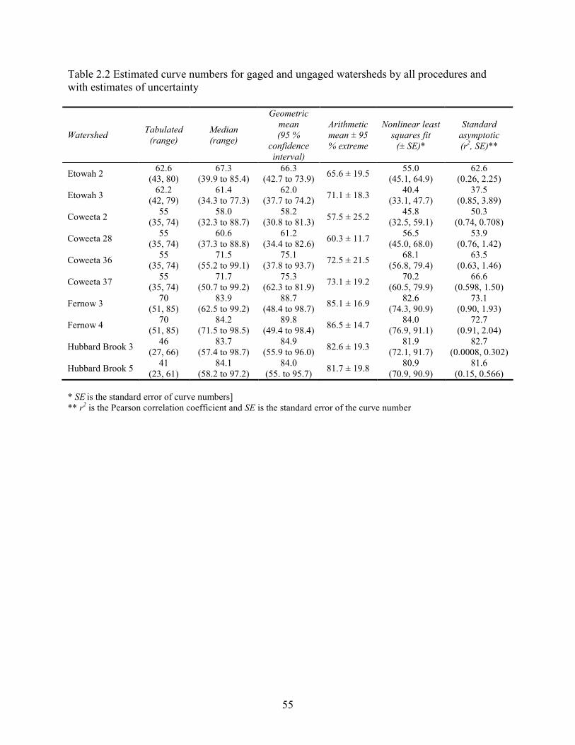
55

Table 2.2 Estimated curve numbers for gaged and ungaged watersheds by all procedures and with estimates of uncertainty

Watershed Tabulated

(range)

Median

(range)

Geometric

mean

(95 %

confidence

interval)

Arithmetic

mean ± 95

% extreme

Nonlinear least

squares fit

(± SE)*

Standard

asymptotic

(r2, SE)**

Etowah 2 62.6

(43, 80) 67.3

(39.9 to 85.4) 66.3

(42.7 to 73.9) 65.6 ± 19.5

55.0 (45.1, 64.9)

62.6 (0.26, 2.25)

Etowah 3 62.2

(42, 79) 61.4

(34.3 to 77.3) 62.0

(37.7 to 74.2) 71.1 ± 18.3

40.4 (33.1, 47.7)

37.5 (0.85, 3.89)

Coweeta 2 55

(35, 74) 58.0

(32.3 to 88.7) 58.2

(30.8 to 81.3) 57.5 ± 25.2

45.8 (32.5, 59.1)

50.3 (0.74, 0.708)

Coweeta 28 55

(35, 74) 60.6

(37.3 to 88.8) 61.2

(34.4 to 82.6) 60.3 ± 11.7

56.5 (45.0, 68.0)

53.9 (0.76, 1.42)

Coweeta 36 55

(35, 74) 71.5

(55.2 to 99.1) 75.1

(37.8 to 93.7) 72.5 ± 21.5

68.1 (56.8, 79.4)

63.5 (0.63, 1.46)

Coweeta 37 55

(35, 74) 71.7

(50.7 to 99.2) 75.3

(62.3 to 81.9) 73.1 ± 19.2

70.2 (60.5, 79.9)

66.6 (0.598, 1.50)

Fernow 3 70

(51, 85) 83.9

(62.5 to 99.2) 88.7

(48.4 to 98.7) 85.1 ± 16.9

82.6 (74.3, 90.9)

73.1 (0.90, 1.93)

Fernow 4 70

(51, 85) 84.2

(71.5 to 98.5) 89.8

(49.4 to 98.4) 86.5 ± 14.7

84.0 (76.9, 91.1)

72.7 (0.91, 2.04)

Hubbard Brook 3 46

(27, 66) 83.7

(57.4 to 98.7) 84.9

(55.9 to 96.0) 82.6 ± 19.3

81.9 (72.1, 91.7)

82.7 (0.0008, 0.302)

Hubbard Brook 5 41

(23, 61) 84.1

(58.2 to 97.2) 84.0

(55. to 95.7) 81.7 ± 19.8

80.9 (70.9, 90.9)

81.6 (0.15, 0.566)

* SE is the standard error of curve numbers] ** r2 is the Pearson correlation coefficient and SE is the standard error of the curve number

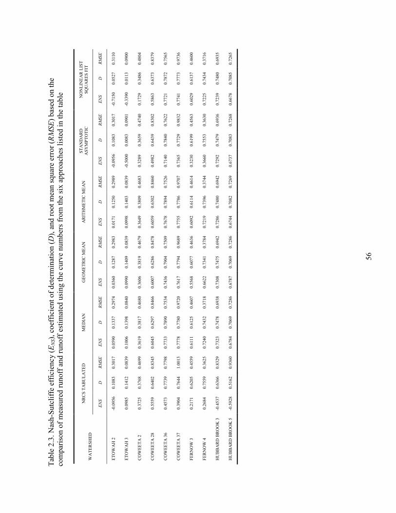
56

Table 2.3. Nash-Sutcliffe efficiency (ENS), coefficient of determination (D), and root mean square error (RMSE) based on the

comparison of measured runoff and runoff estim

ated using the curve numbers from the six approaches listed in the table

NRCS TABULATED

MEDIA

N

GEOMETRIC M

EAN

ARITHMETIC M

EAN

STANDARD

ASYMPTOTIC

NONLIN

EAR LIST

SQUARES FIT

WATERSHED

ENS

D

RMSE

ENS

D

RMSE

ENS

D

RMSE

ENS

D

RMSE

ENS

D

RMSE

ENS

D

RMSE

ETOWAH 2

-0.0956

0.1083

0.3017

0.0590

0.1337

0.2974

0.0360

0.1287

0.2983

0.0171

0.1250

0.2989

-0.0956

0.1083

0.3017

-0.7150

0.0527

0.3110

ETOWAH 3

0.0985

0.1412

0.0839

0.1006

0.1398

0.0840

0.0990

0.1409

0.0839

0.0998

0.1403

0.0839

-0.5000

0.0083

0.0901

-0.3390

0.0113

0.0900

COWEETA 2

0.3725

0.3768

0.4699

0.3619

0.3817

0.4680

0.3606

0.3819

0.4679

0.3649

0.3809

0.4683

0.3289

0.3659

0.4740

0.1729

0.3486

0.4804

COWEETA 28

0.5559

0.6402

0.8345

0.6045

0.6297

0.8466

0.6007

0.6286

0.8478

0.6059

0.6302

0.8460

0.4982

0.6439

0.8302

0.5863

0.6373

0.8379

COWEETA 36

0.4573

0.7739

0.7798

0.7733

0.7890

0.7534

0.7436

0.7904

0.7509

0.7678

0.7894

0.7526

0.7140

0.7840

0.7622

0.7721

0.7872

0.7565

COWEETA 37

0.3904

0.7644

1.0013

0.7778

0.7780

0.9720

0.7617

0.7794

0.9689

0.7755

0.7786

0.9707

0.7365

0.7729

0.9832

0.7741

0.7773

0.9736

FERNOW 3

0.2171

0.6205

0.4559

0.6111

0.6125

0.4607

0.5568

0.6077

0.4636

0.6092

0.6114

0.4614

0.3230

0.6199

0.4563

0.6029

0.6137

0.4600

FERNOW 4

0.2684

0.7559

0.3625

0.7240

0.7432

0.3718

0.6622

0.7341

0.3784

0.7219

0.7396

0.3744

0.3660

0.7553

0.3630

0.7225

0.7434

0.3716

HUBBARD BROOK 3

-0.4537

0.6366

0.8329

0.7323

0.7478

0.6938

0.7308

0.7475

0.6942

0.7286

0.7480

0.6942

0.7292

0.7479

0.6936

0.7239

0.7480

0.6935

HUBBARD BROOK 5

-0.5928

0.5162

0.9360

0.6784

0.7069

0.7286

0.6787

0.7069

0.7286

0.6744

0.7082

0.7269

0.6737

0.7083

0.7268

0.6678

0.7085

0.7265

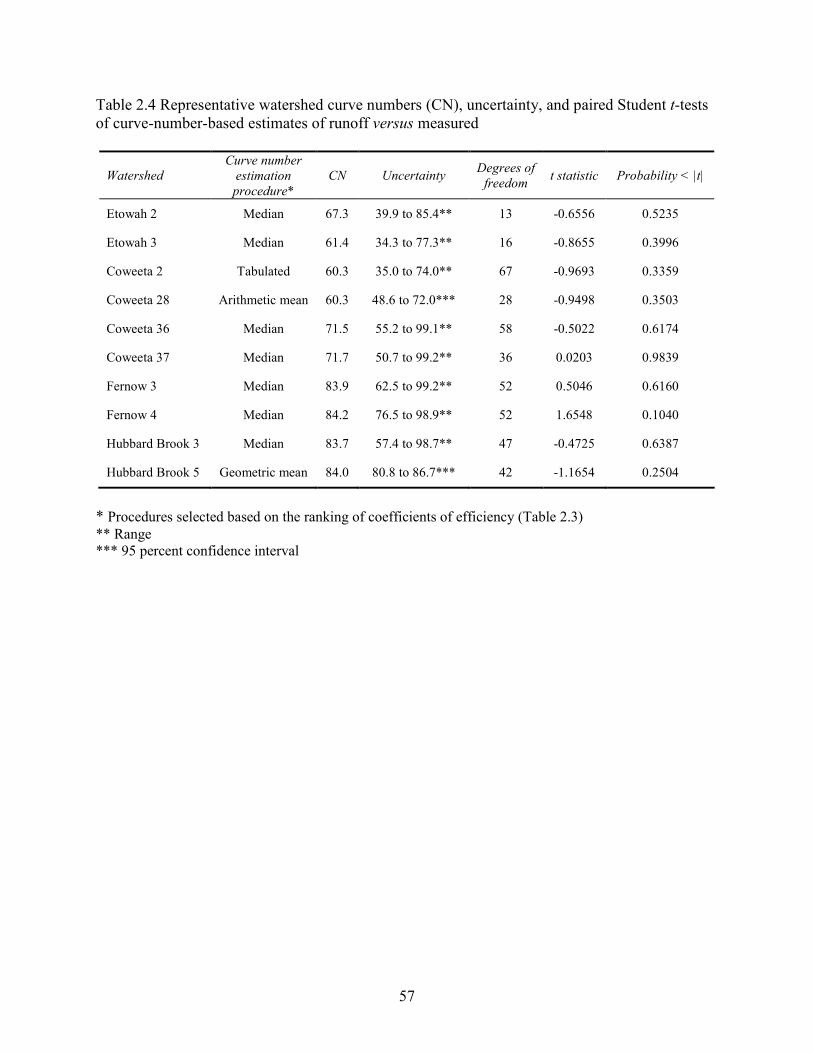
57

Table 2.4 Representative watershed curve numbers (CN), uncertainty, and paired Student t-tests of curve-number-based estimates of runoff versus measured

Watershed

Curve number

estimation

procedure*

CN Uncertainty Degrees of

freedom t statistic Probability < |t|

Etowah 2 Median 67.3 39.9 to 85.4** 13 -0.6556 0.5235

Etowah 3 Median 61.4 34.3 to 77.3** 16 -0.8655 0.3996

Coweeta 2 Tabulated 60.3 35.0 to 74.0** 67 -0.9693 0.3359

Coweeta 28 Arithmetic mean 60.3 48.6 to 72.0*** 28 -0.9498 0.3503

Coweeta 36 Median 71.5 55.2 to 99.1** 58 -0.5022 0.6174

Coweeta 37 Median 71.7 50.7 to 99.2** 36 0.0203 0.9839

Fernow 3 Median 83.9 62.5 to 99.2** 52 0.5046 0.6160

Fernow 4 Median 84.2 76.5 to 98.9** 52 1.6548 0.1040

Hubbard Brook 3 Median 83.7 57.4 to 98.7** 47 -0.4725 0.6387

Hubbard Brook 5 Geometric mean 84.0 80.8 to 86.7*** 42 -1.1654 0.2504

* Procedures selected based on the ranking of coefficients of efficiency (Table 2.3) ** Range *** 95 percent confidence interval

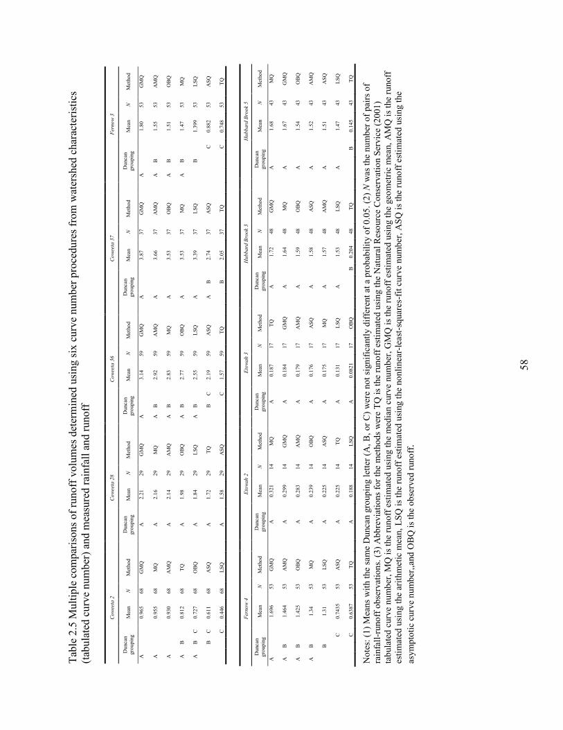
58

Table 2.5 M

ultiple comparisons of runoff volumes determined using six curve number procedures from watershed characteristics

(tabulated curve number) and m

easured rainfall and runoff

Coweeta 2

Coweeta 28

Coweeta 36

Coweeta 37

Fernow 3

Duncan

grouping

Mean

N

Method

Duncan

grouping

Mean

N

Method

Duncan

grouping

Mean

N

Method

Duncan

grouping

Mean

N

Method

Duncan

grouping

Mean

N

Method

A

0.965

68

GMQ

A

2.21

29

GMQ

A

3.14

59

GMQ

A

3.87

37

GMQ

A

1.80

53

GMQ

A

0.955

68

MQ

A

2.16

29

MQ

A

B

2.92

59

AMQ

A

3.66

37

AMQ

A

B

1.55

53

AMQ

A

0.930

68

AMQ

A

2.14

29

AMQ

A

B

2.83

59

MQ

A

3.53

37

OBQ

A

B

1.51

53

OBQ

A

B

0.812

68

TQ

A

1.98

29

OBQ

A

B

2.77

59

OBQ

A

3.53

37

MQ

A

B

1.47

53

MQ

A

B

C

0.727

68

OBQ

A

1.84

29

LSQ

A

B

2.55

59

LSQ

A

3.39

37

LSQ

B

1.399

53

LSQ

B

C

0.611

68

ASQ

A

1.72

29

TQ

B

C

2.19

59

ASQ

A

B

2.74

37

ASQ

C

0.882

53

ASQ

C

0.446

68

LSQ

A

1.58

29

ASQ

C

1.57

59

TQ

B

2.05

37

TQ

C

0.748

53

TQ

Fernow 4

Etowah 2

Etowah 3

Hubbard Brook 3

Hubbard Brook 5

Duncan

grouping

Mean

N

Method

Duncan

grouping

Mean

N

Method

Duncan

grouping

Mean

N

Method

Duncan

grouping

Mean

N

Method

Duncan

grouping

Mean

N

Method

A

1.696

53

GMQ

A

0.321

14

MQ

A

0.187

17

TQ

A

1.72

48

GMQ

A

1.68

43

MQ

A

B

1.464

53

AMQ

A

0.299

14

GMQ

A

0.184

17

GMQ

A

1.64

48

MQ

A

1.67

43

GMQ

A

B

1.425

53

OBQ

A

0.283

14

AMQ

A

0.179

17

AMQ

A

1.59

48

OBQ

A

1.54

43

OBQ

A

B

1.34

53

MQ

A

0.239

14

OBQ

A

0.176

17

ASQ

A

1.58

48

ASQ

A

1.52

43

AMQ

B

1.31

53

LSQ

A

0.225

14

ASQ

A

0.175

17

MQ

A

1.57

48

AMQ

A

1.51

43

ASQ

C

0.7435

53

ASQ

A

0.225

14

TQ

A

0.131

17

LSQ

A

1.53

48

LSQ

A

1.47

43

LSQ

C

0.6387

53

TQ

A

0.188

14

LSQ

A

0.0821

17

OBQ

B

0.204

48

TQ

B

0.145

43

TQ

Notes: (1) Means with the same Duncan grouping letter (A

, B, or C) were not significantly different at a probability of 0.05. (2) N was the number of pairs of

rainfall-runoff observations. (3) Abbreviations for the methods were TQ is the runoff estim

ated using the Natural Resource Conservation Service (2001)

tabulated curve number, MQ is the runoff estim

ated using the median curve number, GMQ is the runoff estim

ated using the geometric mean, AMQ is the runoff

estimated using the arithmetic m

ean, LSQ is the runoff estim

ated using the nonlinear-least-squares-fit curve number, ASQ is the runoff estim

ated using the

asymptotic curve number,,and OBQ is the observed runoff.

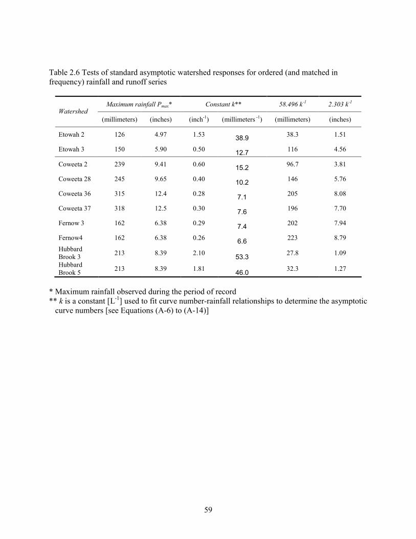
59

Table 2.6 Tests of standard asymptotic watershed responses for ordered (and matched in frequency) rainfall and runoff series

Maximum rainfall Pmax*

Constant k** 58.496 k-1 2.303 k

-1

Watershed

(millimeters) (inches) (inch-1) (millimeters -1) (millimeters) (inches)

Etowah 2 126 4.97 1.53 38.9

38.3 1.51

Etowah 3 150 5.90 0.50 12.7

116 4.56

Coweeta 2 239 9.41 0.60 15.2

96.7 3.81

Coweeta 28 245 9.65 0.40 10.2

146 5.76

Coweeta 36 315 12.4 0.28 7.1

205 8.08

Coweeta 37 318 12.5 0.30 7.6

196 7.70

Fernow 3 162 6.38 0.29 7.4

202 7.94

Fernow4 162 6.38 0.26 6.6

223 8.79

Hubbard Brook 3

213 8.39 2.10 53.3

27.8 1.09

Hubbard Brook 5

213 8.39 1.81 46.0

32.3 1.27

* Maximum rainfall observed during the period of record ** k is a constant [L-1] used to fit curve number-rainfall relationships to determine the asymptotic curve numbers [see Equations (A-6) to (A-14)]

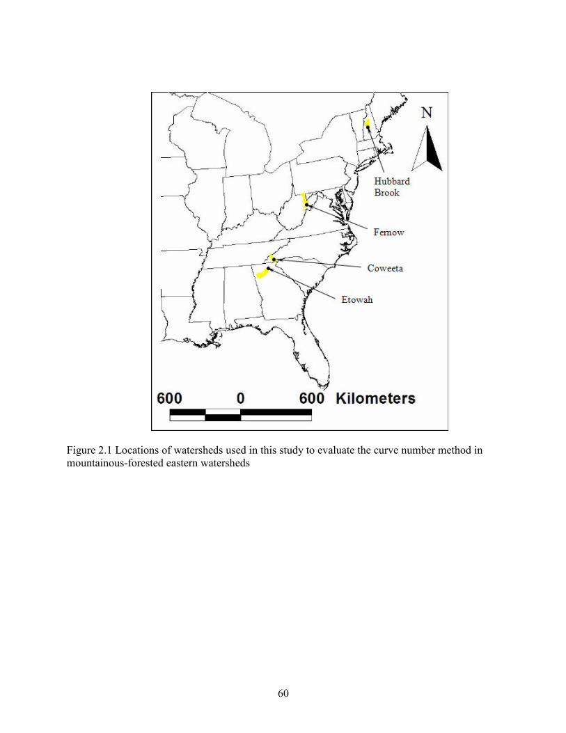
60

Figure 2.1 Locations of watersheds used in this study to evaluate the curve number method in mountainous-forested eastern watersheds

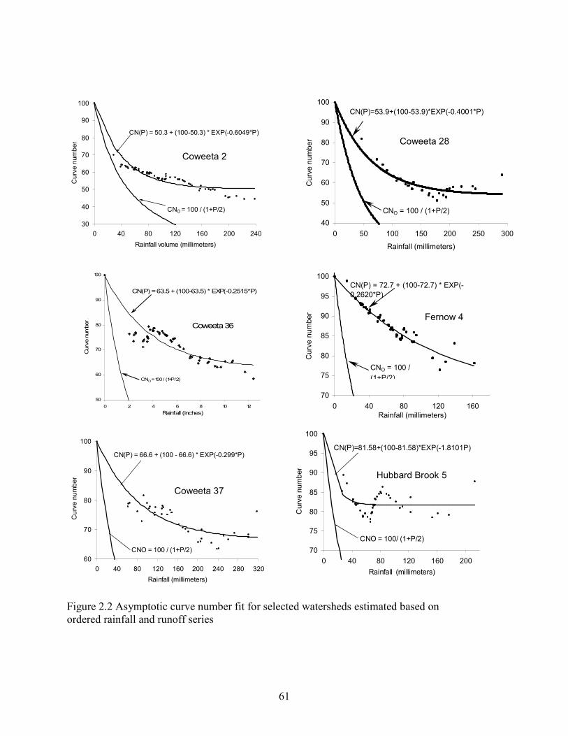
61

30

40

50

60

70

80

90

100

0 40 80 120 160 200 240

Rainfall volume (millimeters)

Curve number

CN(P) = 50.3 + (100-50.3) * EXP(-0.6049*P)

CNO = 100 / (1+P/2)

50

60

70

80

90

100

0 2 4 6 8 10 12

Rainfall (inches)

Curve number …..

CN(P) = 63.5 + (100-63.5) * EXP(-0.2515*P)

CNO = 100 / (1+P/2)

Coweeta 36

60

70

80

90

100

0 40 80 120 160 200 240 280 320

Rainfall (millimeters)

Curve number

CN(P) = 66.6 + (100 - 66.6) * EXP(-0.299*P)

CNO = 100 / (1+P/2)

40

50

60

70

80

90

100

0 50 100 150 200 250 300

Rainfall (millimeters)

Curve number

CN(P)=53.9+(100-53.9)*EXP(-0.4001*P)

CNO = 100 / (1+P/2)

70

75

80

85

90

95

100

0 40 80 120 160

Rainfall (millimeters)

Curve number

CN(P) = 72.7 + (100-72.7) * EXP(-

0.2620*P)

CNO = 100 /

(1+P/2)

70

75

80

85

90

95

100

0 40 80 120 160 200

Rainfall (millimeters)

Curve number

CN(P)=81.58+(100-81.58)*EXP(-1.8101P)

CNO = 100/ (1+P/2)

Figure 2.2 Asymptotic curve number fit for selected watersheds estimated based on ordered rainfall and runoff series

Coweeta 2

Coweeta 28

Coweeta 37

Coweeta 28

Hubbard Brook 5

Coweeta 28

Coweeta 28

Fernow 4

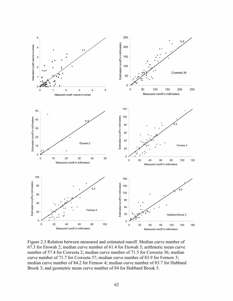
62

0

1

2

3

4

5

0 1 2 3 4 5

Measured runoff volume in inches

Estim

ated runoff volume in inches……….

1:1

0

10

20

30

40

50

0 10 20 30 40 50

Measured runoff in millimeters

Estimated runoff in m

illimeters.

1:1

Etowah 2

0

20

40

60

80

100

0 20 40 60 80 100

Measured runoff in millimeters

Estimated runoff in m

illimeters.

1:1

Fernow 4

0

50

100

150

200

250

0 50 100 150 200 250

Measured runoff in millimeters

Estimated runoff in m

illimeters

1:1

Coweeta 36

0

20

40

60

80

100

120

0 20 40 60 80 100 120

Measured runoff in millimeters

Estimated runoff in m

illimeters.

1:1

Fernow 3

0

30

60

90

120

150

180

0 30 60 90 120 150 180

Measured runoff in millimeters

Estimated runoff in m

illimeters

1:1

Hubbard Brook 3

Figure 2.3 Relation between measured and estimated runoff. Median curve number of 67.3 for Etowah 2; median curve number of 61.4 for Etowah 3; arithmetic mean curve number of 57.4 for Coweeta 2; median curve number of 71.5 for Coweeta 36; median curve number of 71.7 for Coweeta 37; median curve number of 83.9 for Fernow 3; median curve number of 84.2 for Fernow 4; median curve number of 83.7 for Hubbard Brook 3; and geometric mean curve number of 84 for Hubbard Brook 5.

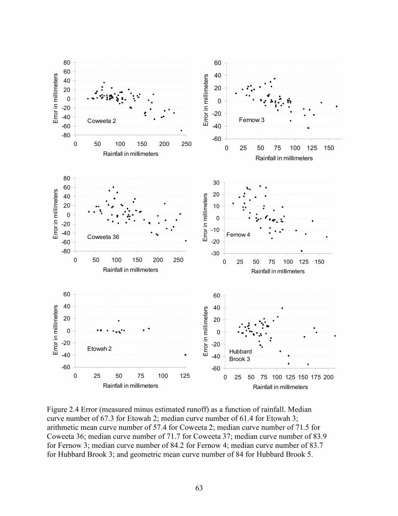
63

-80

-60

-40

-20

0

20

40

60

80

0 50 100 150 200 250

Rainfall in millimeters

Error in m

illimeters

Coweeta 2

-80

-60

-40

-20

0

20

40

60

80

0 50 100 150 200 250

Rainfall in millimeters

Error in m

illimeters

Coweeta 36

-60

-40

-20

0

20

40

60

0 25 50 75 100 125

Rainfall in millimeters

Error in m

illimeters

Etowah 2

-60

-40

-20

0

20

40

60

0 25 50 75 100 125 150

Rainfall in millimeters

Error in m

illimeters

Fernow 3

-30

-20

-10

0

10

20

30

0 25 50 75 100 125 150

Rainfall in millimeters

Error in m

illimeters

Fernow 4

-60

-40

-20

0

20

40

60

0 25 50 75 100 125 150 175 200

Rainfall in millimeters

Error in m

illimeters

Hubbard

Brook 3

Figure 2.4 Error (measured minus estimated runoff) as a function of rainfall. Median curve number of 67.3 for Etowah 2; median curve number of 61.4 for Etowah 3; arithmetic mean curve number of 57.4 for Coweeta 2; median curve number of 71.5 for Coweeta 36; median curve number of 71.7 for Coweeta 37; median curve number of 83.9 for Fernow 3; median curve number of 84.2 for Fernow 4; median curve number of 83.7 for Hubbard Brook 3; and geometric mean curve number of 84 for Hubbard Brook 5.

64

CHAPTER 3

EFFECTS OF SEASONAL VARIATION AND FOREST HARVESTING ON

RUNOFF FROM TEN, SMALL, MOUNTAINOUS, FORESTED

WATERSHEDS IN THE EASTERN UNITED STATES2

2 Negussie Tedela, Steven McCutcheon, Todd Rasmussen, Rhett Jackson, Earnest W. Tollner, Wayne Swank, John

Campbell, and Mary B. Adams. To be submitted to the Journal of the American Water Resources Association.

65

Abstract

Dormant and growing seasons should affect runoff-rainfall relationships for deciduous

forests. However, the Natural Resource Conservation Service curve number method does not

explicitly consider seasonal variation in estimating runoff. In addition, many studies indicate that

streamflow increases after forest harvest because of the decreases in evapotranspiration. No

evidence exists, however, that resulting streamflow increases can be translated to a difference in

curve numbers between the preharvest and hydrologic effect periods. This study evaluated the

effects of seasonal variation and forest harvest practices on curve numbers derived using annual

maximum series of observed rainfall and runoff for forested watersheds. The investigation used

three pairs of watersheds, including three with undisturbed forest cover, to investigate these

effects. The analysis partitioned observed rainfall and runoff according to the dormant and

growing seasons and separately into preharvest and hydrologic effect periods. Curve numbers

calibrated for the growing seasons seem to be smaller than those for the dormant seasons for all

watersheds. the variances of growing-season curve numbers for three of the six watersheds were

significantly different from that of the dormant season with transition periods included, while

four of the six watersheds showed significant difference when the transition periods were

excluded from the analysis. Curve numbers specific to the growing and dormant seasons are

recommended for each watershed. The paired studies suggest that forest harvesting would

definitely increase streamflow and curve numbers. However, the increase in curve number is not

significant for some of the treatments because of the effect on curve number is much more

variable than the effect on total annual flow and may even be inverted in some years or in some

seasons. In most cases, the periods of clearcutting effects are too short to accurately relate any

66

forest management practice to changes in curve numbers compared to longer preharvest and

control watershed records.

Keywords: Curve number, dormant and growing seasons, forest harvesting, runoff-rainfall

relationship, watershed, forest, runoff modeling, hydrology, gaged watersheds,

ungaged watersheds,

Forested watershed response to seasons and harvest

The curve number method is widely used for estimating runoff because of the

convenience and simplicity. The effect of seasonal variation on runoff volume has not been

explicitly incorporated in the curve number method and as a result ignores the impact of seasonal

variation of evapotranspiration and interception. The method uses a constant value of initial

abstraction (Ia) equaling 20 percent of the potential maximum retention, which is may not be

appropriate for both dormant and growing seasons. Jacobs and Srinivasan (2005) pointed out a

need for seasonal applications of the method. Runoff estimation with annually consistent

parameters has limited application because watershed response varies substantially between

seasons. For example, the seasonal tank model by Paik et al. (2005) successfully simulated

runoff with less error compared to the non-seasonal model. In the southeastern United States,

more than half of the land area is forested, and evapotranspiration from forested watersheds can

vary from 85 percent of annual rainfall in coastal Florida to 50 percent in the cool southern

Appalachian Mountains (Sun et al., 2002). In general, forests have larger evapotranspiration

rates than nonirrigated agricultural or urban landscapes. Varying the curve number on a seasonal

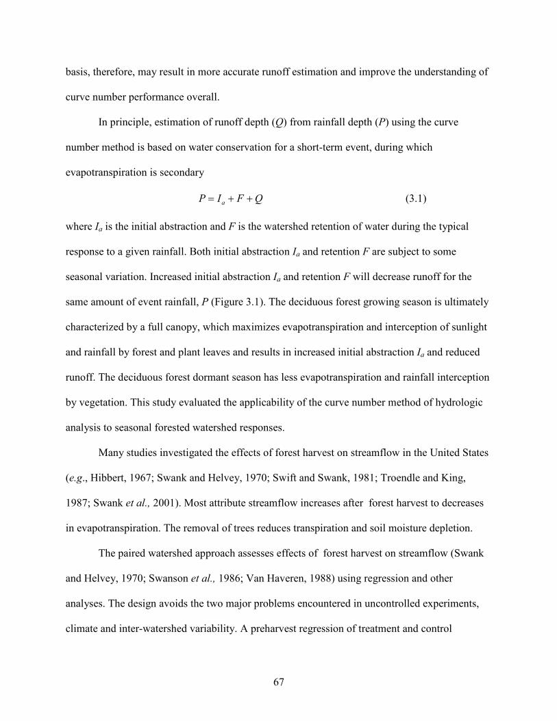
67

basis, therefore, may result in more accurate runoff estimation and improve the understanding of

curve number performance overall.

In principle, estimation of runoff depth (Q) from rainfall depth (P) using the curve

number method is based on water conservation for a short-term event, during which

evapotranspiration is secondary

QFIP a ++= (3.1)

where Ia is the initial abstraction and F is the watershed retention of water during the typical

response to a given rainfall. Both initial abstraction Ia and retention F are subject to some

seasonal variation. Increased initial abstraction Ia and retention F will decrease runoff for the

same amount of event rainfall, P (Figure 3.1). The deciduous forest growing season is ultimately

characterized by a full canopy, which maximizes evapotranspiration and interception of sunlight

and rainfall by forest and plant leaves and results in increased initial abstraction Ia and reduced

runoff. The deciduous forest dormant season has less evapotranspiration and rainfall interception

by vegetation. This study evaluated the applicability of the curve number method of hydrologic

analysis to seasonal forested watershed responses.

Many studies investigated the effects of forest harvest on streamflow in the United States

(e.g., Hibbert, 1967; Swank and Helvey, 1970; Swift and Swank, 1981; Troendle and King,

1987; Swank et al., 2001). Most attribute streamflow increases after forest harvest to decreases

in evapotranspiration. The removal of trees reduces transpiration and soil moisture depletion.

The paired watershed approach assesses effects of forest harvest on streamflow (Swank

and Helvey, 1970; Swanson et al., 1986; Van Haveren, 1988) using regression and other

analyses. The design avoids the two major problems encountered in uncontrolled experiments,

climate and inter-watershed variability. A preharvest regression of treatment and control

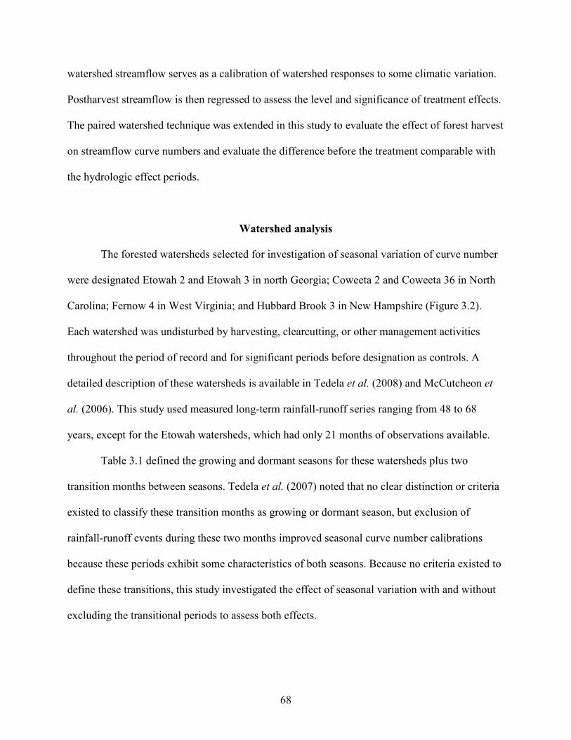
68

watershed streamflow serves as a calibration of watershed responses to some climatic variation.

Postharvest streamflow is then regressed to assess the level and significance of treatment effects.

The paired watershed technique was extended in this study to evaluate the effect of forest harvest

on streamflow curve numbers and evaluate the difference before the treatment comparable with

the hydrologic effect periods.

Watershed analysis

The forested watersheds selected for investigation of seasonal variation of curve number

were designated Etowah 2 and Etowah 3 in north Georgia; Coweeta 2 and Coweeta 36 in North

Carolina; Fernow 4 in West Virginia; and Hubbard Brook 3 in New Hampshire (Figure 3.2).

Each watershed was undisturbed by harvesting, clearcutting, or other management activities

throughout the period of record and for significant periods before designation as controls. A

detailed description of these watersheds is available in Tedela et al. (2008) and McCutcheon et

al. (2006). This study used measured long-term rainfall-runoff series ranging from 48 to 68

years, except for the Etowah watersheds, which had only 21 months of observations available.

Table 3.1 defined the growing and dormant seasons for these watersheds plus two

transition months between seasons. Tedela et al. (2007) noted that no clear distinction or criteria

existed to classify these transition months as growing or dormant season, but exclusion of

rainfall-runoff events during these two months improved seasonal curve number calibrations

because these periods exhibit some characteristics of both seasons. Because no criteria existed to

define these transitions, this study investigated the effect of seasonal variation with and without

excluding the transitional periods to assess both effects.

69

The observed rainfall and runoff series divided according to the two seasons, resulted in a

watershed series of curve numbers (CN) based on

( ) 105425

1000

21

2 +

+−+

=PQQQP

CN (3.2a)

or

( ) 2545425

400,25

21

2 +

+−+

=PQQQP

CN . (3.2b)

where the measured rainfall (P) and direct runoff (Q) from individual storm events were in

inches for Equation (3.4a) or millimeters for Equation (3.4b). This study arithmetically averaged

the curve numbers for each season to estimate a mean for the growing season and a mean for the

dormant season.

This investigation compared the mean curve numbers for the growing season (CNg) to the

mean curve numbers of the dormant season (CNd) with and without transition periods using the

analysis of variance (ANOVA) at the 0.05 level of significance. The null and alternative were

• Null hypothesis: no significant difference existed between curve numbers for the

growing and dormant seasons

• Alternative hypothesis: a significant difference existed between curve numbers for the

two seasons

The application of the analysis of variance rejected the null hypotheses if the calculated

probability was less than the level of significance. The alternative hypothesis was accepted if the

probability was greater than 0.05.

This study analyzed paired Coweeta 36 and Coweeta 37, Fernow 3 and Fernow 4, and

Hubbard Brook 3 and Hubbard Brook 5 to determined the hydrologic effect periods from previous

70

studies and hence to investigate the effect of forest harvesting on curve number. Coweeta 36,

Fernow 4, and Hubbard Brook 3 were control watersheds; while Coweeta 37, Fernow 3, and

Hubbard Brook 5 watersheds are treated watersheds (Table 3.2).

All woody vegetation was cut on the 43.7-hectare (108.0-acre) Coweeta 37 and left on

the ground to avoid any hydrologic effect of road and landing construction in 1963 (Table 3.2).

The U.S. Forest Service had partially cut 31.7-hectares (78.3-acres) from Fernow 3 in 1969,

leaving only trees 2.5-centimeters (1-inch) in diameter at breast height or smaller and without

disturbing a 3-hectare (7.4-acre) protective strip extending approximately 20 meters (66 feet)

along each side of the stream channel. Careful construction of logging roads provided efficient

harvesting of forest products without harming other resources (Patric, 1980) and demonstrated

best management practices for West Virginia and other states. Prior to this 1969 diameter limit

cut, 13 percent, 8 percent, and 6 percent of the basal area was harvested intensively in 1958,

1963, and 1967, respectively (Table 3.2). Hubbard Brook 5 was clearcut during the winter of late

1983 and early 1984. The U.S. Forest Service harvested all trees greater than 5 centimeters (2

inches) in diameter at breast height and removed both boles and branches from the watershed

with skidders (Table 3.2). A feller-buncher harvested all accessible trees with hydraulic shears;

while on steeper slopes, chainsaws were used (McCutcheon et al., 2006).

The paired watershed analysis of Coweeta 36 and 37 revealed that water yields changed

due to the tree cutting during 1963 to 1973 and water yields returned to preharvest in 1974

(Patric, 1980). In comparison with the paired hydrologic control of Fernow 4, Fernow 3 water

yields during the preharvest period of 1951 to 1956 were not remarkably different from those

yields measured during and after the diameter limit cuts of 1958, 1963, and 1967. However,

water yields increased from 1969 to 1975 due to the 1969 and 1972 clearcutting, defining a

71

distinct period of hydrologic effects (Patric, 1980). Hydrologic effects for Hubbard Brook 5 of

only one year in duration increased soil moisture and, as a result, maximum flows increased 40

percent. Summer peak flows increased 20 percent (Hornbeck et al., 1997).

Rainfall-runoff pairs separated into preharvest and hydrologic effect series, were the basis

for computing curve numbers for each event from which the means were derived separately for

preharvest and hydrologic effect periods for all treated watersheds. The curve numbers for the

preharvest period (CNpt) was compared to the curve numbers of the hydrologic effect periods

(CNhe), using the analysis of variance (ANOVA) at the 0.05 level of significance. The null and

alternative hypotheses were

• Null hypothesis: no significant difference existed between curve numbers for the

preharvest and hydrologic effects periods

• Alternative hypothesis: a significant difference existed between curve numbers for the

two periods

Seasonal and harvest effects

Curve numbers computed for the growing seasons were smaller than for the dormant

seasons for all watersheds, in both cases whether the transition periods were included or

excluded (Figures 3.3 and 3.4, and Table 3.3). Coweeta 2 and Etowah 3 have the largest and

smallest variations in curve numbers, respectively. The difference between the dormant and

growing season curve numbers for Etowah 3 was only 2.7 when the transition periods are

included and 5.4 when the transition periods were excluded (Table 3.3). The difference between

the dormant and growing season curve numbers for Coweeta 2 was 14.1 when the transition

periods were included and 11.6 when the transition periods were excluded. Excluding the

72

transitional months increased the variation in dormant and growing season curve numbers for

Coweeta 36, Etowah 3, and Hubbard Brook 3.

The analysis of variance (Tables 3.4 and 3.5) showed that the mean curve numbers of the

growing seasons computed from only three of the six watersheds were significantly different

from that of the dormant season mean curve numbers at the 0.05 level of significance. The effect

of the seasonal transitions on the analysis was ambiguous. If the transitions were included in the

analysis, the dormant and growing season curve numbers for Coweeta 2, Coweeta 36, and

Fernow 4 were significantly different. The dormant and growing season curve numbers for

Coweeta 2, Fernow 4, and Hubbard Brook 3 were significantly different with the transitions

excluded from the analysis. The insignificant difference between the seasonal curve numbers for

Etowah 2 and Etowah 3 is probably due to the limited 21-month records. Although the curve

numbers for Coweeta 2 and Fernow 4 were clearly seasonal, the indications of seasonality for

Coweeta 36 and Hubbard Brook 3 were ambiguous. In addition, the asymptotic curve numbers of

the growing and the dormant seasons showed numerical difference (Figure 3.6) for Coweeta 2.

However, the curve number and rainfall datasets were not suitable to fit a standard asymptotic

curve number equation and are not shown here.

Curve numbers computed for the preharvest period are smaller than for the hydrologic

effect period for all six watersheds some of the differences are insignificant (Table 3.6 and

Figure 3.5). The differences between mean curve numbers computed for preharvest and

hydrologic effect periods are 8.4 and 16.6 for Coweeta 37 and Hubbard Brook 5, respectively.

For Fernow 3, the preharvest mean curve number differed from the mean curve number

computed for the period including the diameter limit harvests of 1958, 1963, and 1967 by 8.1.

The preharvest mean differed with the mean for the hydrologic effect period that included the

73

partial clearcutting of 1969 and 1972 by 3.6 (Table 3.6). Hubbard Brook 5 and Fernow 3 had the

largest and smallest differences in curve numbers between the hydrologic effect and preharvest

periods, respectively.

The analysis of variance (Table 3.7) showed that preharvest mean curve number for

Coweeta 37 and mean curve number for the hydrologic effect period (1963 to 1973) were

significantly different at the 0.05-level of significance. The preharvest mean curve number for

the Fernow 3 and the mean curve number determined during the forest harvest of 13 percent, 8

percent, and 6 percent of the basal area in 1958, 1963, and 1968, respectively, were also

significantly different at the 0.05 level of significance. However, the Fernow 3 mean curve

number measured during the hydrologic effects of clearcutting in 1969 and 1972 was not

significantly different (at the 0.05 level of significance) from the preharvest mean curve number

(Figures 3.5 and Table 3.7).

Hornbeck et al. (1997) could only distinguish an effect of the Hubbard Brook 5

clearcutting on annual water yield in water year 1984, but the maximum annual storm of was

clearly an exceptional event. The 1984 maximum runoff was exceptional compared to the

maximum rainfall of that year. This 1984 exceptional event produced the largest curve number

calculated for any annual maximum rainfall-runoff event for the 49-year record. The fewer years

of record available to calculate curve numbers, the more imprecision increases and the greater

the chance that these short periods have sets of curve numbers that are statistically different.

Greater runoff curve numbers observed after forest harvest showed that runoff estimates

would also be greater for a particular watershed compared to the runoff estimate before the

treatment periods [see Equations (3.1) and (3.2)].

74

Conclusions

Three of six watersheds showed significant curve number differences between the

growing and dormant seasons. The insignificant effect of seasonal variation for some of the

watersheds was attributed to the variability of curve numbers. Therefore, runoff estimation with

annually consistent curve numbers has limited application because the watershed response may

vary seasonally.

Paired studies at three watersheds showed that forest harvesting increased streamflow

and, hence, curve numbers. However, the increase in curve number was not significant for the

Fernow 3 clearcutting. Large observed uncertainties were consistent with results by Hibbert

(1967), who found the hydrological response to forest harvests highly variable and, for the most

part, unpredictable. This variability was reflected id the great uncertainty observed in the curve

numbers. Furthermore, gains in streamflow, as Swank and Helvey (1970) described, are only

temporary since regrowth offsets changes in evapotranspiration brought about by the initial

cutting.

Acknowledgments

Financial assistance provided in part by (1) the West Virginia Division of Forestry, (2)

the U.S. Geological Survey through the Georgia Water Resources Institute, and (3) the Warnell

School of Forest and Natural Resources. Richard Hawkins of the University of Arizona, Tucson

provided insightful background and guidance on the use, interpretation, and limitations of the

curve number method. The observed watershed characteristics and rainfall-runoff series required

for this study were provided by Wayne Swank and Stephanie Laseter from the U.S. Forest

Service Coweeta Hydrologic Laboratory; Frederica Wood, from the U.S. Forest Service Fernow

75

Timber and Watershed Laboratory; John Campbell, from the U.S. Forest Service Hubbard Brook

Experimental Forest; and Josh Romeis from the University of Georgia Etowah Research Project.

References

Hawkins, R. H. 1998. Local sources for runoff curve numbers. Eleventh Annual Symposium of

the Arizona Hydrological Society, September 23-26, Tucson, Arizona.

Hibbert, A. R. 1967. Forest treatment effects on water yield. In: International Symposium on

Forest Hydrology, Sopper, W. E. and Lull, H. W. (Eds.), Proceedings of a National

Science Foundation Advanced Science Seminar, Pergamon Press, New York, New York,

527–543.

Hornbeck, J. W., C. W. Martin, and C. Eagar. 1997. Summary of water yield experiments at

Hubbard Brook Experimental Forest, New Hampshire. Canadian Journal of Forest

Research 27: 2043-2052.

Jacobs, J. H. and R. Srinivasan. 2005. Effects of curve number modification on runoff estimation

using WSR-88D rainfall data in Texas watersheds. Journal of Soil and Water

Conservation 60(5): 274-278.

McCutcheon, S. C., Tedela N. H., Adams, M. B., Swank, W., Campbell, J. L., Hawkins, R. H.,

Dye, C. R. 2006. Rainfall-runoff relationships for selected Eastern U.S. forested

mountain watersheds: Testing of the curve number method for flood analysis. Report

prepared for the West Virginia Division of Forestry, Charleston, West Virginia.

Paik, K., J. H. Kim, H. S. Kim, and D. R. Lee. 2005. A conceptual rainfall-runoff model

considering seasonal variation. Hydrological Processes 19: 3837-3850.

76

Patric, J. H. 1980. Effects of wood products harvest on forest soil and water relations. Journal of

Environmental Quality 9(1): 73-80.

Sun, G., S. G. McNulty, D. M. Amatya, R. W. Skaggs, L. W. Swift, J. P. Shepard, and H.

Riekerk. 2002. A comparison of the hydrology of the coastal forested wetlands/pine

flatwoods and the mountainous uplands in the Southern U.S. Journal of Hydrology

263(1-4): 92-104.

Swank, W. T. and J. D. Helvey. 1970. Reduction of streamflow increases following regrowth of

clearcut hardwood forests. In Symposium on the Results of Research on Representative

and Experimental Basins, International Association of Scientific Hydrology and United

Nations Educational, Scientific and Cultural Organization, Wellington, New Zealand,

346-360.

Swank, W. T., J. M. Vose, and K. J. Elliott. 2001. Long-term hydrologic and water quality

responses following commercial clearcutting of mixed hardwoods on a southern

Appalachian catchment. Forest Ecology and Management 143(1-3): 163–178.

Swanson, R. H., D. L. Golding, R. L. Rothwell, and P. Y. Bernier. 1986. Hydrologic effects of

clear-cutting at Marmot Creek and Streeter watersheds, Alberta. Northern Forestry Center

Information Report NOR-X-278, Canadian Forestry Service, Edmonton, Alberta,

Canada, 27 pp.

Swift, L. W. and W. T. Swank. 1981. Long term responses of stream-flow following clearcutting

and regrowth. Hydrological Sciences Bulletin 26(3): 245-256.

Tedela, N. H., T. C. Rasmussen, and S. C. McCutcheon. 2007. Effects of seasonal variation on

runoff curve number for selected watersheds of Georgia -- preliminary study, In

77

Proceedings of the 2007 Georgia Water Resources Conference, March 27-29, University

of Georgia, Athens.

Troendle, C. A. and R. M. King. 1987. The effect of partial and clearcutting on streamflow at

Deadhorse Creek, Colorado. Journal of Hydrology 90(1-2): 145-157.

Van Haveren, B. P. 1988. A reevaluation of the Wagon Wheel Gap forest watershed experiment.

Forest Science 34: 208-214.

Van Mullein, J. A., D. E. Woodward, R. H. Hawkins, and A. T. Hjelmfelt. 2002. Runoff curve

number method: Beyond the handbook. In Hydrologic Modeling for the 21st Century,

Second Federal Interagency Hydrologic Modeling Conference, July 28-August 1, U.S.

Geological Survey Advisory Committee on Water Information, Las Vegas, Nevada.

78

Table 3.1 Dormant and growing seasons

Seasons Watershed

Growing Dormant

Transition periods

Coweeta 2 May to October November to April April to May, October to November

Coweeta 36 May to October November to April April to May, October to November

Etowah 2 April to October November to March March to April, October to November

Etowah 3 April to October November to March March to April, October to November

Fernow 4 May to October November to April April to May, October to November

Hubbard Brook 3 May 16 to September 15 September 16 to May 15 April 15 to May 30, September 16 to October 30

79

Table 3.2 Preharvest and hydrologic effect periods for the three-paired watersheds

Watershed Treatment

Area

(hectares)

Total period

of record

(years)

Preharvest

period (years)

Hydrologic

effect period

(years)

Fernow 3 Diameter limit cutting (1958, 1963, 1967), clearcut (1969, 1972)

34.3 53 1951 to 1957 (7 years)

1969 to 1975 (7 years)

Fernow 4 Control 38.7 49 N/A N/A

Coweeta 36 Control 46.6 59 N/A N/A

Coweeta 37 Clearcut (1963) 43.7 37

1944 to

1947, 1949

to 1951,

1953 to

1957, 1962

(13 years)*

1963 to 1973 (11 years)

Hubbard Brook 3 Control 42.4 41 N/A N/A

Hubbard Brook 5 Clearcut during the winter of late 1983 and early 1984

21.9 43 1962 to 1982 (21 years)

Mid-1983 to mid-1984 (1 year)

* Coweeta Hydrologic Laboratory did not collect runoff data during the 1948, 1952, and 1958 to 1961 water years.

80

Table 3.3 Differences in dormant and growing season mean curve numbers including and

excluding transitions periods

Including transition months Excluding transition months

Watershed Season

Mean Difference Mean Difference

Growing 48.4 50.1 Coweeta 2

Dormant 62.5

14.1

61.7

11.6

Growing 67.5 68.2

Coweeta 36

Dormant 74.8

7.3

76.2

7.9

Growing 65.3 7.0 64.3 5.4

Etowah 2

Dormant 72.3 69.8

Growing 63.1 58.9

Etowah 3

Dormant 65.8

2.7

64.1

5.2

Growing 80.9 81.5

Fernow 4

Dormant 89.7

8.8

89.3

7.8

Growing 80.3 80.3

Hubbard Brook 3

Dormant 84.6

4.3

89.5

9.2

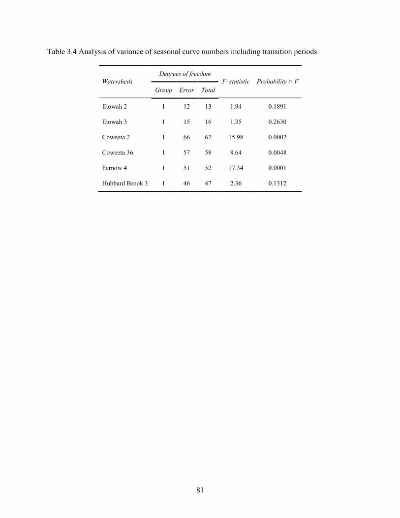
81

Table 3.4 Analysis of variance of seasonal curve numbers including transition periods

Degrees of freedom

Watersheds

Group Error Total

F- statistic Probability > F

Etowah 2 1 12 13 1.94 0.1891

Etowah 3 1 15 16 1.35 0.2630

Coweeta 2 1 66 67 15.98 0.0002

Coweeta 36 1 57 58 8.64 0.0048

Fernow 4 1 51 52 17.34 0.0001

Hubbard Brook 3 1 46 47 2.36 0.1312

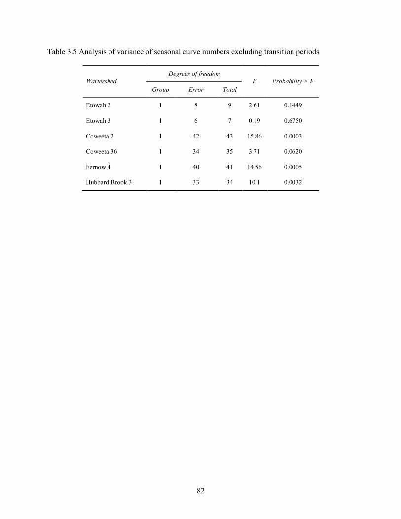
82

Table 3.5 Analysis of variance of seasonal curve numbers excluding transition periods

Degrees of freedom Wartershed

Group Error Total

F Probability > F

Etowah 2 1 8 9 2.61 0.1449

Etowah 3 1 6 7 0.19 0.6750

Coweeta 2 1 42 43 15.86 0.0003

Coweeta 36 1 34 35 3.71 0.0620

Fernow 4 1 40 41 14.56 0.0005

Hubbard Brook 3 1 33 34 10.1 0.0032

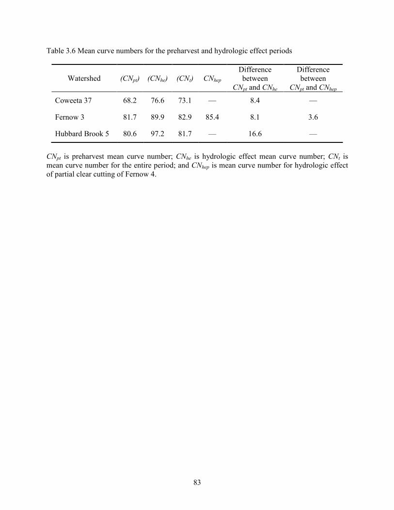
83

Table 3.6 Mean curve numbers for the preharvest and hydrologic effect periods

Watershed (CNpt) (CNhe) (CNt) CNhep

Difference between

CNpt and CNhe

Difference between

CNpt and CNhep

Coweeta 37 68.2 76.6 73.1 — 8.4 —

Fernow 3 81.7 89.9 82.9 85.4 8.1 3.6

Hubbard Brook 5 80.6 97.2 81.7 — 16.6 —

CNpt is preharvest mean curve number; CNhe is hydrologic effect mean curve number; CNt is mean curve number for the entire period; and CNhep is mean curve number for hydrologic effect of partial clear cutting of Fernow 4.

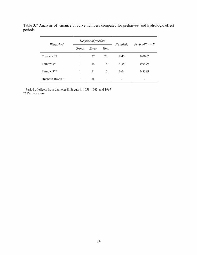
84

Table 3.7 Analysis of variance of curve numbers computed for preharvest and hydrologic effect periods

Degrees of freedom Watershed

Group Error Total

F statistic Probability > F

Coweeta 37 1 22 23 8.45 0.0082

Fernow 3* 1 15 16 4.55 0.0499

Fernow 3** 1 11 12 0.04 0.8389

Hubbard Brook 3 1 0 1 - -

* Period of effects from diameter limit cuts in 1958, 1963, and 1967 ** Partial cutting

85

Figure 3.1 Water balance for a short-term rainfall event in which P is rainfall, Q is runoff depth, Ia is initial abstraction, F is retention, and S is potential maximum retention.

Q

Ia

F

P

S

86

a) Etowah watersheds

b) Coweeta watersheds

2

28

36

37

87

c) Fernow watersheds

d) Hubbard Brook watersheds

Figure 3.2 Study watersheds

88

Watersheds

Coweeta 2 Coweeta 36 Etowah 2 Etowah 3 Fernow 4 Hubbard B. 3

Curve Number

0

20

40

60

80

Growing

Dormant

Figure 3.3 Curve numbers for growing and dormant seasons including transition periods

89

Watersheds

Coweeta 2 Coweeta 36 Etowah 2 Etowah 3 Fernow 4 Hubbard B. 3

Curve Number

0

20

40

60

80

Growing

Dormant

Figure 3.4 Curve numbers for growing and dormant seasons excluding transition periods

90

Watersheds

Coweeta 37 Fernow 3 Hubbard Brook 5

Curve number

40

50

60

70

80

90

100

Curve number for the pretreatment period

Curve number for the hydrologic effect period

Curve number for the entire record period

Curve number for the hydrologic effect of partial clearcutting of Fernow 3

Figure 3.5 Comparison of mean curve numbers for the three watersheds before tree harvest, during hydrologic effects, and for the entire record

91

20

30

40

50

60

70

80

90

100

0 1 2 3 4 5 6 7 8 9 10

Rainfall Volume in inches

Curve number....

Dormant season

Growing season

CN(P)=47+(100-47)*EXP(-0.3305*P)

CNO = 100/ (1+P/2)

CN(P)=33.5+(100-33.5)*EXP(-0.4250*P)

Figure 3.6 Asymptotic curve numbers for growing and dormant seasons of Coweeta 2

92

CHAPTER 4

RAINFALL AND RUNOFF PROBABILITY DISTRIBUTIONS FOR FOUR, SMALL,

FORESTED WATERSHEDS IN THE MOUNTAINOUS, EASTERN UNITED STATES3

3 Negussie Tedela, Steven McCutcheon, Todd Rasmussen. To be submitted to the Journal of the Hydrologic Engineering

93

Abstract

This study investigated probability distributions for annual-maximum rainfall and runoff

observations to evaluate the distributions of estimated runoff volumes based on the Natural

Resource Conservation Service curve number method. The observations of rainfall and runoff

volumes occurred at four forested experimental watersheds in the mountains of North Carolina,

West Virginia, and New Hampshire. Goodness-of-fit tests defined the appropriate cumulative

probability distribution for each series of annual-maximum rainfall or runoff. This study applied

the Cramer-von Mises and Anderson-Darling goodness–of-fit tests to select appropriate rainfall

and runoff distributions for each watershed. The gamma distribution was appropriate for all

observed rainfall and runoff volumes, except for the Hubbard Brook 3 rainfall observations. The

Weibull distribution was best for estimated runoff volumes from all the watersheds except for

Hubbard Brook 3. The lognormal distribution best matches the estimated runoff volume from

Hubbard Brook 3. Differences between the distributions of the estimated and observed, annual-

maximum runoff volumes demonstrate the weakness of the Natural Resources Conservation

Service curve number method. The estimated runoff volumes of Coweeta 2 are in agreement

with the observed runoff for average conditions (50 percent probability of occurrence or two-

year return period). For the rest of the three watersheds, the tabulated curve number seems to

yield runoff that occurred once every one hundred years. The tabulated curve number may yield

runoff for events occurring rarely and under-estimate runoff for the rest of the distribution. The

results showed the bias that could occur in using the tabulated curve number method for these

watersheds.

94

Keywords: Curve number, runoff-rainfall relationship, normal, runoff modeling, probability,

return periods, lognormal distribution, gamma distribution, and Weibull

distribution, goodness of fit, chi-square, Kolmogorov-Smirnov, Cramer-von Mises,

Anderson-Darling, forested watershed, mountains, hydrology, gaged watersheds,

ungaged watersheds

Introduction

Based on the prior applications by Pilgrim and Cordery (1993) and Schaake et al. (1967)

to peak flows, Hjelmfelt (1980) assumed that ordering and matching of the annual-maximum

rainfall and runoff volumes by probabilities is the best method to determine the probability

distribution. Hawkins et al. (2005) and Schneider and McCuen (2005) used this method because

the joint frequency of an event rainfall volume and the event runoff volume has been ignored in

most hydrologic design problems. However, independent ranking of rainfall and runoff decreases

the quantifiable uncertainty in the determination of curve numbers and runoff distributions and

thus can be misleading but not necessarily inaccurate (McCutcheon et al., 2006).

This study independently ranked the observed, annual-maximum rainfall and runoff

volumes and estimated runoff volumes to determine cumulative probability distributions for four

small, forested watersheds in the mountains of the eastern United States. The tabulated curve

numbers of the Natural Resource Conservation Service were the basis of the runoff estimates.

The objectives were to (1) apply goodness-of-fit tests for hypothesis testing and assess whether

various probability distributions were consistent with the observations, (2) examine the

probability distributions of the observed and estimated runoff volumes to asses how well these

distributions match for various return periods.

95

Matching probability distributions to represent observations or estimates involved testing

the measurements for independence and origination from identical populations (Chin, 2006).

Before the advent of widespread electronic computing, hydrologists plotted and visually matched

different continuous probability distributions to observations. The current (2009) art is to apply

goodness-of-fit hypothesis-testing to match various probability distributions (Appendix) with the

measurements, consistent with the underlying process generating the measured rainfall or runoff

(Chin, 2006).

Some goodness-of-fit tests only determine if the observed or estimated, annual-maximum

rainfall or runoff comes from a normally distributed population, which rarely occurs in

hydrologic analysis. The more general tests used in hydrology (Hann, 2002) are discussed in the

following paragraphs.

The chi-square test (Snedecor and Cochran, 1989) determines if a series of observations

or estimates came from a population with type of distribution. The chi-square (χ2) goodness-of-

fit statistic is

( )∑=

−=

k

i i

ii

E

EO

1

2

2χ (4.1)

where k is the total number of classes of bins, Oi is the observed frequency for class i, and Ei is

the expected frequency for class i. For this test, the investigator classifies observations or

estimates by putting the information put into defined classes that have been called bins (from the

industrial process of sorting size products into containers). One limitation is that the chi-square

statistic depends on how the observations or estimates are classified. Another limitation is that

the method requires each class have five or greater observations or estimates for the chi-square

approximation to be valid.

96

The Kolmogorov-Smirnov test (Chakravart et al., 1967) also determines if a sample

comes from a population with a specific distribution but the maximum discrepancy between

observations and a specific empirical distribution is the basis. The Kolmogorov-Smirnov statistic

(D) for a given distribution function F(x) and a distribution from observations or estimates, Fn (x)

is

( ) ( )xFxFD n −= max (4.2)

where max indicates the maximum discrepancy. The Weibull empirical distribution is one

function that cannot be assessed using Kolmogorov-Smirnov statistic. Mathematically the test is

similar to the Kolmogorov test.

The Cramer-von Mises statistic W2 (Anderson, 1962) is used for judging the goodness-

of-fit of a probability distribution F* compared to a given distribution F(x), and is found using:

( ) ( )[ ] ( )xdFxFxFW

2

*2 ∫∞

∞−

−= (4.3)

Tests may involve unclassified estimates or observations. Also, this test is satisfactory for

symmetric and skewed distributions.

The Anderson-Darling test (Stephens, 1974) is a modification of the Kolmogorov-

Smirnov test used to test if a series of observations or estimates came from a population with a

specific empirical distribution. This test gives more weight to the tails of a distribution than does

the Kolmogorov-Smirnov test. The Anderson-Darling (A2) statistic is

SNA −−=2 (4.4)

where N is the sample size, and

( ) ( ) ( )( )[ ]iNi

N

i

XFXFN

iS −+

=

−+−

=∑ 1

1

1lnln12

(4.5)

97

in which F(Xi) is the cumulative distribution function of the specified distribution, and Xi are the

ordered rainfall or runoff.

Many hydrologists do not use the chi-square and Kolmogorov-Smirnov tests when testing

hydrologic frequency distributions, because of their lack of sensitivity to low-frequency events

and the large probability of accepting the hypothesis when the hypothesis is actually false (Haan,

2002). The chi-square test is further limited to having at least five observations or estimates

within each class or class interval (Hann, 2002). Furthermore, the chi-square statistic loses

information in a test of a continuous distribution by grouping estimates into classes (Chakravarti

et al., 1967). The Cramer-von Mises and Anderson-Darling statistics are superior to the

Kolmogorov-Smirnov statistic, which is superior to the chi-squared statistic. The Cramer-von

Mises and Anderson-Darling tests make a comparison of two distributions or populations over a

range of data, rather than looking for a marked difference at one point (Chakravarti et al., 1967).

The annual-maximum observed rainfall and observed and estimated runoff series in this study

were not suitable for the chi-square test because of the frequency (the number of occurrences in a

particular class interval) is less than five for some of the classes. Therefore, this investigation

applied the Kolmogorov-Smirnov, Cramer-von Mises, and Anderson-Darling tests, but focused

on the later two superior statistics.

Study watersheds

This study included four watersheds, two from the Coweeta Hydrologic Laboratory,

North Carolina (Coweeta 2 and Coweeta 36), and one watershed each from the Fernow

Experimental Forest, West Virginia (Fernow 4), and the Hubbard Brook Experimental Forest,

New Hampshire (Hubbard Brook 3). These watersheds were controls, which had not been

98

disturbed for many years. The size of watersheds ranged from 12.26 hectares (30.29 acres) to

108.0 hectares (267 acres).

The Coweeta Hydrological Laboratory is located in the Blue Ridge Physiographic

Province of the southern Appalachian Mountains, near Otto, North Carolina. Coweeta 2

elevation ranges from 1,086 to 1,482 meters (3,563 to 4,862 feet). Coweeta 36 elevation ranges

from 710 to 1,010 meters (2,330 feet to 3,314 feet). The Coweeta soil depth averages

approximately 7 meters (23 feet) in depth at lower (Coweeta 2) to mid elevations and is more

shallow (less than 2 meters or 6.6 feet) at high elevations (Coweeta 36) (McCutcheon et al.,

2006). The forest cover includes northern hardwoods, cove hardwoods, xeric oak and pine, oak

and hickory, and mixed oak (USDA, 2004). The Coweeta 2 and 36 controls were uncut and

undisturbed since 1927 but Coweeta 36 was partially defoliated by a fall cankerworm infestation

between 1975 and 1979 (McCutcheon et al., 2006).

The Fernow Experimental Forest lies in the Allegheny Mountain section of the

unglaciated Allegheny Plateau. The Fernow 4 elevations ranged from 735 to 865 meters (2,411

to 2837 feet) over steep slopes. Depths of soils at Fernow are typically 1 meter (3 feet) with 6

centimeters (2.5 inches) of humus. The forest cover included northern red oak, chestnut oak,

white oak, scarlet oak, black oak, and upland oaks (Reinhart et al., 1963). Fernow 4 was last cut

for timber at various times during circa 1905 to 1910 and the watershed was untreated and

undisturbed since May 1, 1951 (McCutcheon et al., 2006).

The Hubbard Brook Experimental Forest was located in the White Mountain National

Forest. The bowl-shaped Hubbard Brook Valley had hilly terrain. Elevation of Hubbard Brook 3

ranges from 522 to 716 meters (1,712 to 2,349 feet). Average stony soil depth of Hubbard Brook

was 50.3 centimeters or 19.8 inches with an average depth of 6.9 centimeters or 2.7 inches of

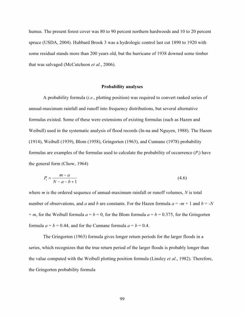
99

humus. The present forest cover was 80 to 90 percent northern hardwoods and 10 to 20 percent

spruce (USDA, 2004). Hubbard Brook 3 was a hydrologic control last cut 1890 to 1920 with

some residual stands more than 200 years old, but the hurricane of 1938 downed some timber

that was salvaged (McCutcheon et al., 2006).

Probability analyses

A probability formula (i.e., plotting position) was required to convert ranked series of

annual-maximum rainfall and runoff into frequency distributions, but several alternative

formulas existed. Some of these were extensions of existing formulas (such as Hazen and

Weibull) used in the systematic analysis of flood records (In-na and Nguyen, 1988). The Hazen

(1914), Weibull (1939), Blom (1958), Gringorten (1963), and Cunnane (1978) probability

formulas are examples of the formulas used to calculate the probability of occurrence (Pi) have

the general form (Chow, 1964)

1+−−−

=baN

amPi (4.6)

where m is the ordered sequence of annual-maximum rainfall or runoff volumes, N is total

number of observations, and a and b are constants. For the Hazen formula a = -m + 1 and b = -N

+ m, for the Weibull formula a = b = 0, for the Blom formula a = b = 0.375, for the Gringorten

formula a = b = 0.44, and for the Cunnane formula a = b = 0.4.

The Gringorten (1963) formula gives longer return periods for the larger floods in a

series, which recognizes that the true return period of the larger floods is probably longer than

the value computed with the Weibull plotting position formula (Linsley et al., 1982). Therefore,

the Gringorten probability formula

100

( )( )12.0

44.0

+−

=N

mPi (4.7)

was selected for this analysis.

For comparison to annual-maximum observations, runoff volumes Q (inches) were

computed from an algebraic rearrangement of the curve number runoff equations as

( )[ ]( )[ ]8008

20022

+−−+

=PCNCN

PCNQ (4.8)

where CN is the curve number tabulated (NRCS, 2001) or calibrated for a particular watershed

and P (inches) is the annual-maximum volume of rainfall. For each rainfall volume and the

watershed curve number, Equation (4.8) produced an estimate of the annual-maximum runoff.

This investigation compared the estimated runoff distribution to the measured rainfall and

measured runoff volumes using the probability distributions that match these observations.

After the ranking of the annual-maximum rainfall and runoff independently for Coweeta

2, Coweeta 36, Fernow 4, and Hubbard Brook 3, this analysis established the probability of

occurrence based on the number of events in each series and the Gringorten probability formula.

This analysis selected the appropriate probability distributions to match the observed rainfall,

observed runoff, and estimated runoff for each watershed based on goodness-of-fit tests. The

quantiles (1, 2, 3, 10, 25, 50, 75, 90, 91, 92, and 99 percent) were determined for the selected

probability distribution; more for the two extremes of the distribution compared to central part of

the distribution. This focuses the statistical assessment at the two extremes where more

variations occur between the observed, annual-maximum rainfall and runoff series and the

selected frequency distributions.

Many probability distributions have been proposed but the lognormal, Weibull, gamma

(Pearson type III), and normal (see the Appendix for definitions) are the most frequently applied

101

in hydrology (Chin, 2006). In this analysis (Figures 4.1 and 4.2), these four distributions were

compared with observed, annual-maximum rainfall and runoff, and estimated, annual-maximum

runoff based on the goodness of fit. The Kolmogorov-Smirnov (D), Cramer-von Mises (W2), and

Anderson-Darling (A2) tests [Equations (4.2), (4.3), and (4.4)] were used for hypothesis testing

where the null (Ho) and alternative (HA) hypotheses were

H0: the stated distribution matched the observations or estimates of annual-maximum

rainfall or runoff

HA: the stated distribution did not match the observations or estimates of annual-

maximum rainfall or runoff

The null hypothesis that a specific distribution matched observations or estimates was rejected if

the probability is less than the significance level (α = 0.05), the probability that the sample could

have been drawn from the population being tested given that the null hypothesis was true. A

probability of 0.05, for example, indicates that would be only a 5 percent chance of drawing the

sample if the null hypothesis was actually true. Probability close to zero signals that the null

hypothesis is false and typically, a difference is very likely to exist.

A comparison of the distributions of measured and estimated, annual-maximum runoff

described whether the magnitude of the selected curve number adequately estimated the

measured runoff volume at various exceedance probabilities. The shape of the computed runoff

volume distribution provided insight into whether the curve number method was applicable to a

particular watershed and for what segments of the measured distribution.

102

Probability distributions

Table 4.1 shows the Kolmogorov-Smirnov, Cramer-von Mises, and Anderson-Darling

tests used to select the cumulative probability distribution that matched the observed, annual-

maximum rainfall from Coweeta 2. The same procedure is used to select the probability

distribution for observed rainfall and runoff volumes and estimated runoff volumes (computed

based on the Natural Resource Conservation Service tabulated curve numbers) for each

watershed. More than one type of probability distributions matched the annual-maximum rainfall

and runoff volumes.

The results of the goodness-of-fit tests for the annual-maximum rainfall series of

Coweeta 2 (Table 4.1) showed that the gamma, lognormal, and Weibull distributions matched

observations, while the normal distribution did not at the 5 percent level of significance. The

Cramer-von Mises and Anderson-Darling statistics are the same for the gamma and Weibull

distributions (Table 4.1). Based on all tests, the probability of accepting the null hypothesis (the

gamma distribution matched the Coweeta 2 observed, annual-maximum rainfall) is more than 50

percent.

The summary of the selected probability distributions together with the scale parameter

(β) and shape parameter (γ) (defined in the Appendix) is in Table 4.2. The gamma distribution

matched the observed, annual-maximum runoff and rainfall volumes for all watersheds except

for the observed rainfall volume on Hubbard Brook 3. The Weibull distribution matched the

estimated, annual-maximum runoff from all the watersheds except for Hubbard Brook 3. The

lognormal distribution matched the observed, annual-maximum rainfall and estimated annual-

maximum runoff for Hubbard Brook 3.

103

The Weibull distribution matched the observed, annual-maximum runoff from Coweeta 2

and Coweeta 36 and observed rainfall of Fernow 4. The lognormal distribution also matched the

observed, annual-maximum rainfall of Coweeta 2 and Coweeta 36 and observed runoff volumes

for Fernow 4 and Hubard Brook 3. For the estimated, annual-maximum runoff volumes from all

watersheds and for observed rainfall volume of Hubbard Brook 3, no other distributions matched

because of the smaller probability of accepting the null hypothesis (Table 4.2).

Figure 4.3 showed that the gamma distribution matched the observed, annual-maximum

rainfall and runoff and the Weibull distribution matched estimated runoff for Coweeta 2.

Although the gamma and Weibull distributions matched the annual-maximum runoff and the

gamma and lognormal distributions matched rainfall for Coweeta 2, this investigation selected

the gamma distribution for consistency. The Coweeta 2 estimated runoff based on the Natural

Resource Conservation Service (2001) tabulated curve number only agreed with the observed

runoff volumes for a return interval of once every three years or frequency of 33 percent.. The

tabulated curve number estimates annual-maximum runoff poorly outside the probabilities

between 55 percent and 20 percent or between 1.8 years and 5 years recurrence interval (Figure

4.3). Thus, the tabulated curve number originally based on the median (probability of 50 percent)

should not be used to estimate design storms of once in 10-years or less frequent, or very

frequent events.

The annual-maximum runoff from Coweeta 36 also matched the gamma and Weibull

distributions and the rainfall the gamma and lognormal distributions. However, this study

selected the gamma distribution for consistency. Figure 4.4 established that the tabulated Natural

Resource Conservation Service (2001) curve number estimated runoff that only agrees at once in

104

one hundred years for Coweeta 36. Practitioners must calibrate curve numbers for these

watersheds to estimate runoff at other return periods.

Figure 4.5 shows the selected gamma distribution matched the observed, annual-

maximum rainfall and runoff and the Weibull distribution matched estimated runoff to a degree

for Fernow 4. The annual-maximum runoff matched the gamma and lognormal distributions and

the rainfall the gamma and Weibull distributions of Fernow 4 but this study selected the gamma

distribution. The estimated runoff based on the tabulated curve number for Fernow 4 watershed

only approached the observed, annual-maximum runoff at a 1 percent probability. However, the

Weibull distribution, the only empirical function in agreement with the estimated runoff,

intersects the gamma distributions matched to the observed runoff at 8 percent probability. The

Weibull distribution overestimates all design runoffs except the 2-year event at a probability of

50 percent that was underestimated. The accuracy of runoff estimation decreased as the

probability of occurrence increased. Practitioners must calibrate the curve number for each

design runoff probability for Fernow 4.

Figure 4.6 showed the annual-maximum distribution of observed rainfall volume,

observed runoff volume, and estimated runoff volume based on tabulated curve number for

Hubbard Brook 3. The lognormal distribution matched the measured, annual-maximum rainfall

and estimated runoff volumes, while the gamma distribution matched the observed runoff for

Hubbard Brook 3. Unlike the other watersheds, in which the gamma distribution matched both

observed, annual-maximum rainfall and runoff volumes, the study selected the lognormal

distribution based on the goodness-of-fit tests to match the observed rainfall volume. The

estimated, annual-maximum runoff based on the tabulated curve number for Hubbard Brook 3

did not come close to any observations (Figure 4.6).

105

Single watershed curve number in doubt

None of the Natural Resource Conservation Service (2001) tabulated curve numbers

estimated accurate runoff from small, mountainous-forested watersheds in the eastern United

States. For all four watersheds investigated, a new curve number is necessary for each important

design storm. Nevertheless, the curve number method--as currently applied--may be too

uncertain to produce tabulations for each design event ranging from once in 2 years to once in

100 years and sometimes longer.

This investigation did not find a single empirical distribution to match the observed,

annual-maximum rainfall and runoff. Although, the gamma distribution matched rainfall and

runoff for all watersheds except for the observed rainfall on the Hubbard Brook 3 watershed, for

which only a lognormal distribution was applicable. Only the Weibull or lognormal distributions

matched estimated runoff based on the tabulated curve numbers.

References

Anderson, T. W. 1962. On the distribution of the two-sample Cramer-von Mises criterion.

Annals of Mathematical Statistics 33(3): 1148-1159.

Blom, G. 1958. Statistical Estimates and Transformed Beta Variables. Wiley, New York, New

York.

Chakravarti, I. M., R. G. Laha, and J. Roy. 1967. Handbook of Methods of Applied Statistics,

Volume I. John Wiley and Sons, 392-394.

Chin, D. A. 2006. Water Resources Engineering. 2nd Ed. Prentice Hall, Upper Saddle River, New

Jersey.

Chow, V. T., ed. 1964. Handbook of Applied Hydrology. McGraw-Hill, New York, New York.

106

Cunnane, C. 1978. Unbiased plotting position - a review. Journal of Hydrology 37(3-4): 205-

222. doi:10.1016/0022-1694(78)90017-3.

Gringorten, I. I. 1963. A plotting rule for extreme probability paper. Journal of Geophysical

Research 68(3) 813-814.

Haan, C. T. 2002. Statistical Methods in Hydrology. Iowa State University Press, Ames.

Hawkins, R. H., E. D. Woodward, J. Ruiyun, J. E. VanMullem, and A. T. Hjelmfelt. 2005.

Runoff Curve Number method: examination of the initial abstraction ratio. ASCE

Watershed Management CN Workshop, Williamsburg, Virginia, originally given at the

Federal Interagency Hydrologic Modeling Conference, July 2002, Las Vegas, Nevada.

Hazen, A. 1914. Storage to be provided in impounding reservoirs for municipal water supply.

Transaction of the American Society of Civil Engineers paper 1308, 77: 1547-1550. (from

Cunnane, 1978).

Hjelmfelt, A. T. 1980. Empirical investigation of curve number techniques. Journal of

Hydraulics Engineering Division, 106(HY9): 1471-1476.

In-na, N. and V. T. A. Nguyen. 1989. An unbiased plotting position formula for the general

extreme value distribution. Journal of Hydrology 106(3-4): 193-209.

McCutcheon, S. C., Tedela N. H., Adams, M. B., Swank, W., Campbell, J. L., Hawkins, R. H.,

Dye, C. R. 2006. Rainfall-runoff relationships for selected Eastern U.S. forested

mountain watersheds: Testing of the curve number method for flood analysis. Report

prepared for the West Virginia Division of Forestry, Charleston, West Virginia.

Pilgrim, D. H. and I. Cordery. 1993. Flood runoff. In Handbook of Hydrology, D. R. Maidment,

ed. McGraw-Hill, New York, New York, Chapter 9: 9.1-9.42.

107

Reinhart, K. G., A. R. Eschner, and G. R. Tremble, Jr. 1963. Effect on streamflow of four forest

practices. U.S. Department of Agriculture Forest Service Research Paper NE-1,

Northeastern Forest Experiment Station, Upper Darby, Pennsylvania.

Schaake, J. C., J. C. Geyer, and J. W. Knapp. 1967. Experimental examination of the rational

method. Journal of the Hydraulics Division 93(HY6): 353-370.

Schneider, L. E. and R. H. McCuen. 2005. Statistical guideline for curve number generation.

Journal of Irrigation and Drainage Engineering 131(3): 282-290.

Snedecor, G. W. and W. G. Cochran. 1989. Statistical Methods. 8th Ed. Iowa State University

Press, Ames.

Stephens, M. A. 1974. EDF statistics for goodness of fit and some comparisons. Journal of the

American Statistical Association 69(347): 730-737.

U.S. Department of Agriculture (USDA). 2004. Experimental forests and ranges of the USDA

Forest Service, General Technical Report NE-321, Northern Research Station, Newtown

Square, Pennsylvania, 178 pp.

Weibull, W. 1939. A statistical theory of strength of materials. Ingenioers vetenskapsakad, 151

pp. (from Hirsch, 1987).

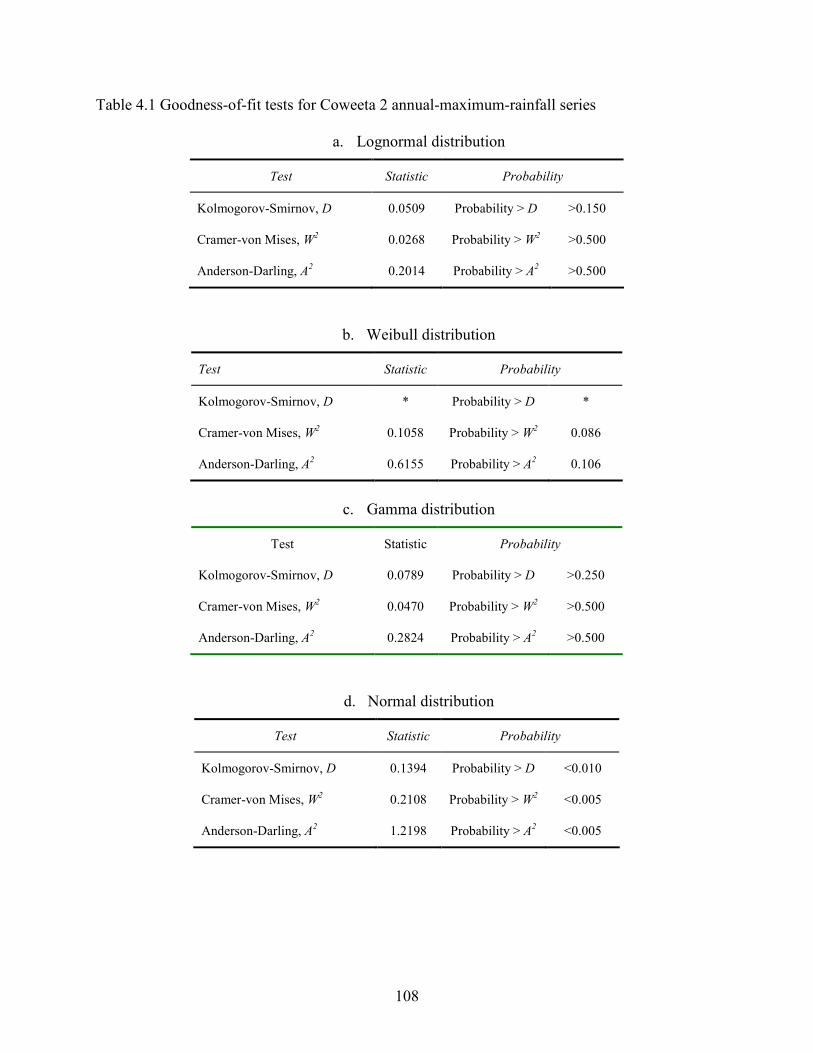
108

Table 4.1 Goodness-of-fit tests for Coweeta 2 annual-maximum-rainfall series

a. Lognormal distribution

Test Statistic Probability

Kolmogorov-Smirnov, D 0.0509 Probability > D >0.150

Cramer-von Mises, W2 0.0268 Probability > W2 >0.500

Anderson-Darling, A2 0.2014 Probability > A2 >0.500

b. Weibull distribution

Test Statistic Probability

Kolmogorov-Smirnov, D * Probability > D *

Cramer-von Mises, W2 0.1058 Probability > W2 0.086

Anderson-Darling, A2 0.6155 Probability > A2 0.106

c. Gamma distribution

Test Statistic Probability

Kolmogorov-Smirnov, D 0.0789 Probability > D >0.250

Cramer-von Mises, W2 0.0470 Probability > W2 >0.500

Anderson-Darling, A2 0.2824 Probability > A2 >0.500

d. Normal distribution

Test Statistic Probability

Kolmogorov-Smirnov, D 0.1394 Probability > D <0.010

Cramer-von Mises, W2 0.2108 Probability > W2 <0.005

Anderson-Darling, A2 1.2198 Probability > A2 <0.005

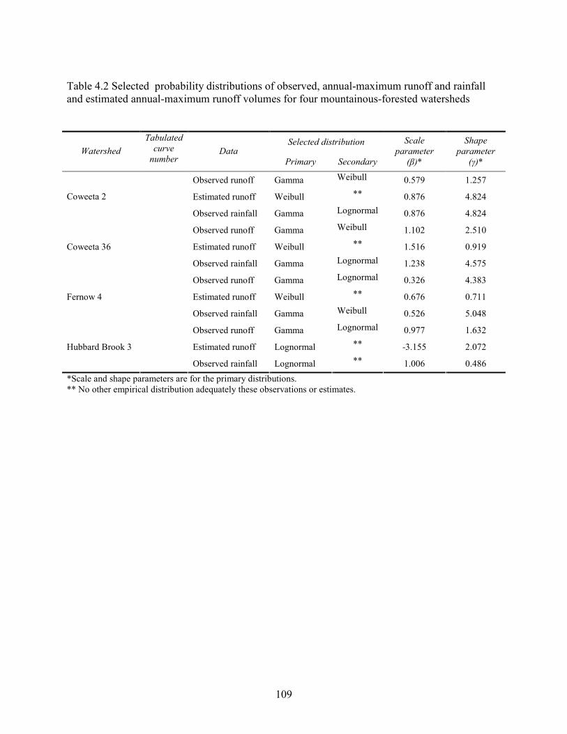
109

Table 4.2 Selected probability distributions of observed, annual-maximum runoff and rainfall and estimated annual-maximum runoff volumes for four mountainous-forested watersheds

Selected distribution Watershed

Tabulated

curve

number Data

Primary Secondary

Scale

parameter

(β)*

Shape

parameter

(γ)*

Observed runoff Gamma Weibull 0.579 1.257

Estimated runoff Weibull ** 0.876 4.824 Coweeta 2

Observed rainfall Gamma Lognormal 0.876 4.824

Observed runoff Gamma Weibull 1.102 2.510

Estimated runoff Weibull ** 1.516 0.919 Coweeta 36

Observed rainfall Gamma Lognormal 1.238 4.575

Observed runoff Gamma Lognormal 0.326 4.383

Estimated runoff Weibull ** 0.676 0.711 Fernow 4

Observed rainfall Gamma Weibull 0.526 5.048

Observed runoff Gamma Lognormal 0.977 1.632

Estimated runoff Lognormal ** -3.155 2.072 Hubbard Brook 3

Observed rainfall Lognormal ** 1.006 0.486

*Scale and shape parameters are for the primary distributions. ** No other empirical distribution adequately these observations or estimates.

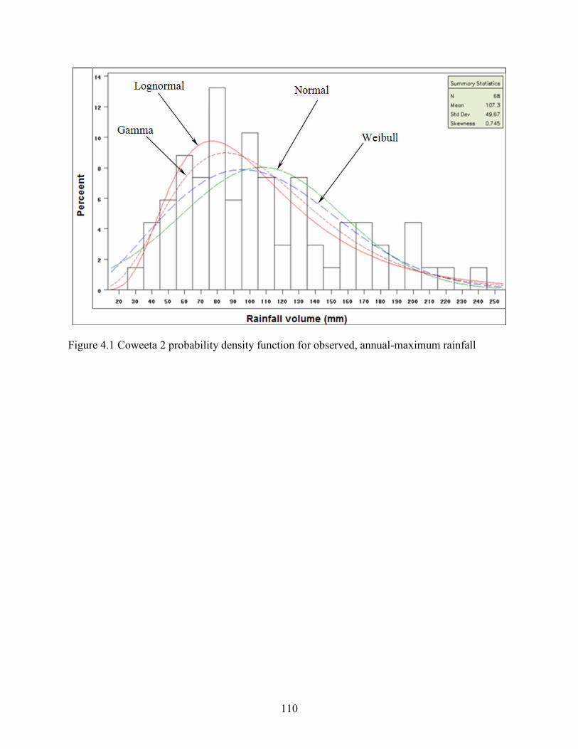
110

Figure 4.1 Coweeta 2 probability density function for observed, annual-maximum rainfall

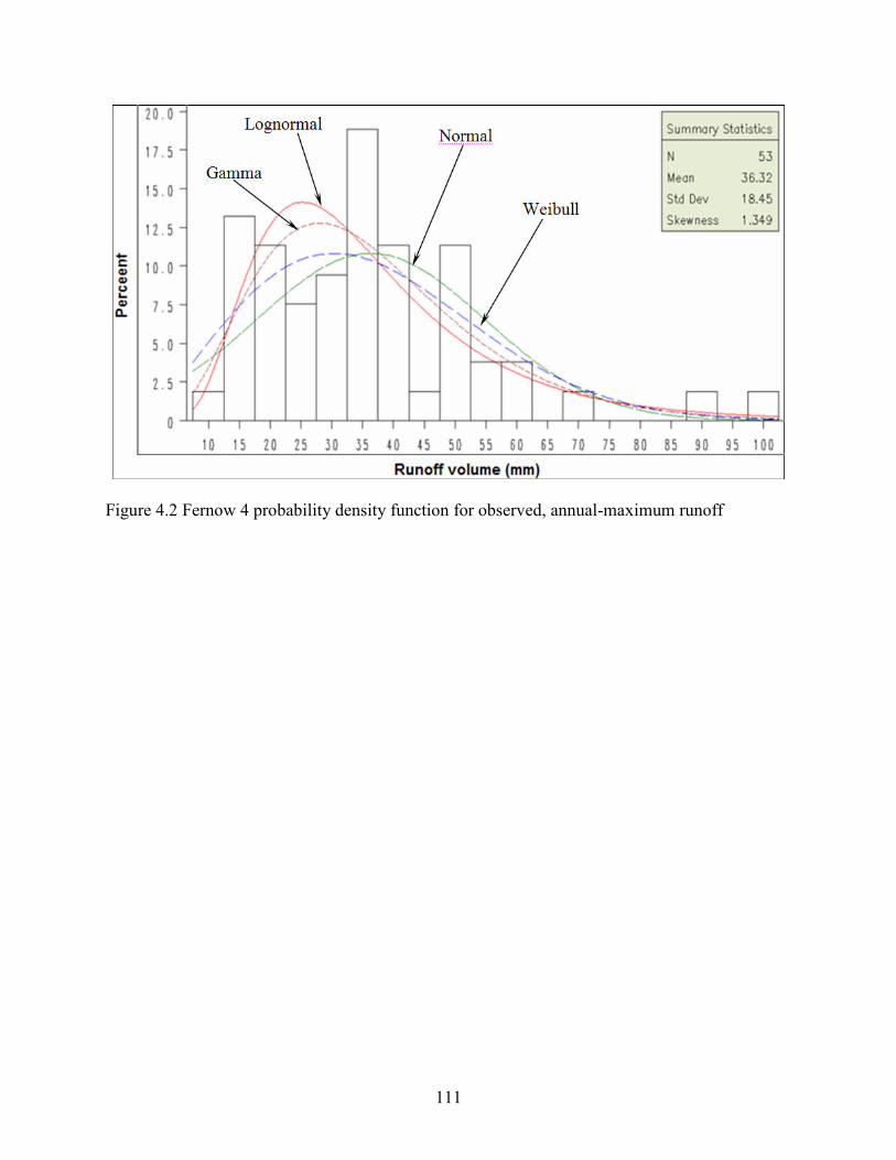
111

Figure 4.2 Fernow 4 probability density function for observed, annual-maximum runoff

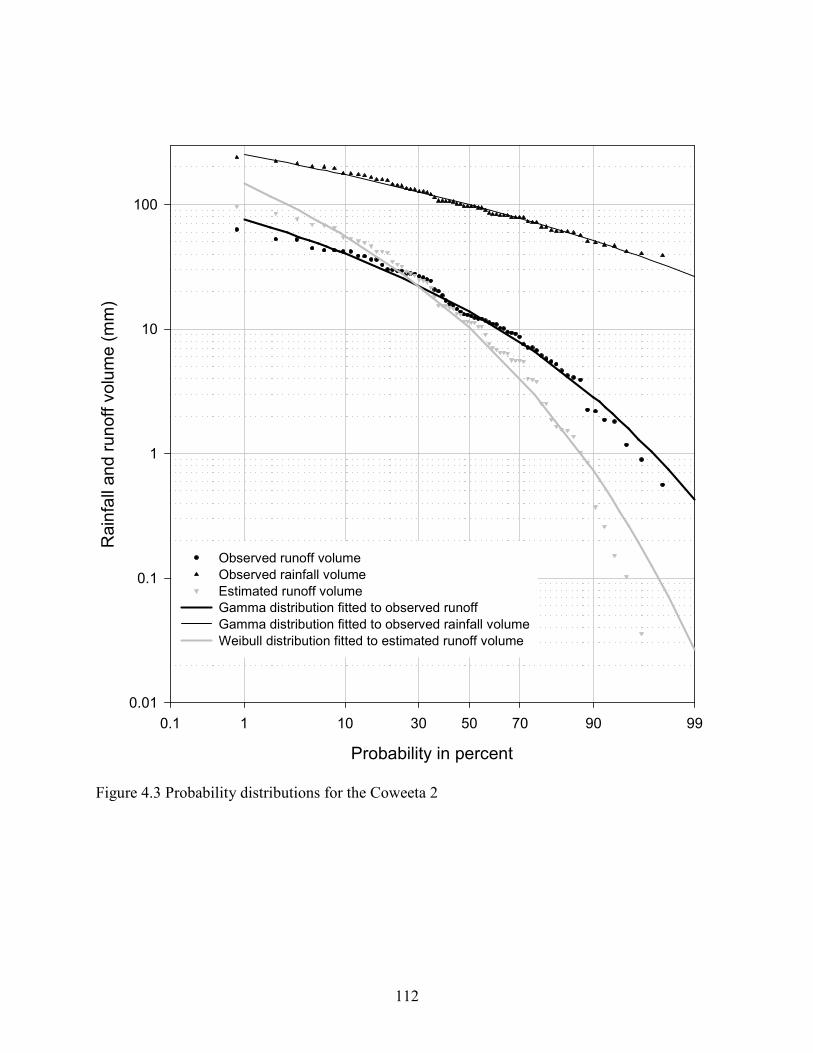
112

Probability in percent

0.1 1 10 30 50 70 90 99

Rainfall and runoff volume (mm)

0.01

0.1

1

10

100

Observed runoff volume

Observed rainfall volume

Estimated runoff volume

Gamma distribution fitted to observed runoff

Gamma distribution fitted to observed rainfall volume

Weibull distribution fitted to estimated runoff volume

Figure 4.3 Probability distributions for the Coweeta 2

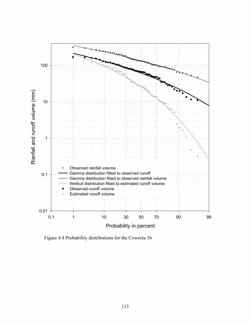
113

Probability in percent

0.1 1 10 30 50 70 90 99

Rianfall and runoff volume (mm)

0.01

0.1

1

10

100

Observed rainfall volume

Gamma distribution fitted to observed runoff

Gamma distribution fitted to observed rainfall volume

Weibull distribution fitted to estimated runoff volume

Observed runoff volume

Estimated runoff volume

Figure 4.4 Probability distributions for the Coweeta 36

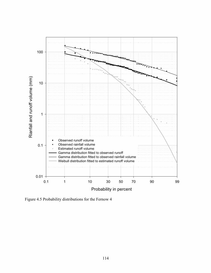
114

Probability in percent

0.1 1 10 30 50 70 90 99

Rianfall and runoff volume (mm)

0.01

0.1

1

10

100

Observed runoff volume

Observed rainfall volume

Estimated runoff volume

Gamma distribution fitted to observed runoff

Gamma distribution fitted to observed rainfall volume

Weibull distribution fitted to estimated runoff volume

Figure 4.5 Probability distributions for the Fernow 4

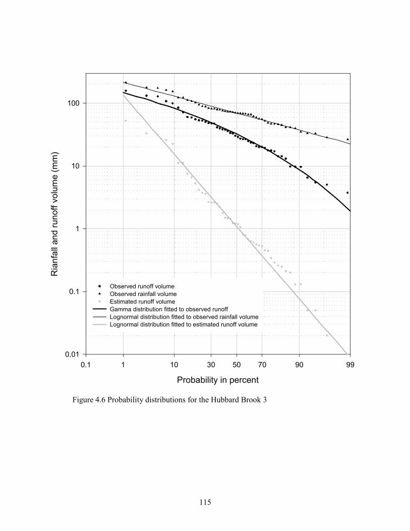
115

Probability in percent

0.1 1 10 30 50 70 90 99

Rianfall and runoff volume (mm)

0.01

0.1

1

10

100

Observed runoff volume

Observed rainfall volume

Estimated runoff volume

Gamma distribution fitted to observed runoff

Lognormal distribution fitted to observed rainfall volume

Lognormal distribution fitted to estimated runoff volume

Figure 4.6 Probability distributions for the Hubbard Brook 3

116

CHAPTER 5

RUNOFF MODELING OF FOUR SMALL, MOUNTAINOUS-FORESTED

WATERSHEDS IN THE EASTERN UNITED STATES USING TOPMODEL4

4 Negussie Tedela, Todd Rasmussen, Steven McCutcheon, John Dowd, Rhett Jackson, Earnest W. Tollner, Wayne

Swank, John Campbell, and Mary B. Adams. To be submitted to the ASCE, Journal of Hydrologic Engineering.

117

Abstract

Runoff responses of four forested watersheds in eastern United States were investigated

using the TOPMODEL, a semi-distributed watershed model that uses topographic information to

simulate runoff at the watershed outlet based on the concepts of saturation excess overland flow

and subsurface flow. The use of the TOPMODEL in single-event runoff modeling is investigated

in this study. The model utilizes a topographic index as an indicator of the likely spatial

distribution of rainfall excess generation in the watershed. The topographic index values within

the watershed are determined using the digital terrain analysis procedures in conjunction with

digital elevation model (DEM) data. Five parameter sets are evaluated on performance of the

runoff prediction using the Generalized Likelihood Uncertainty Estimation (GLUE)

methodology, which involves evaluating many different randomly chosen parameter sets based

on likelihood measures to obtain the best-fit runoff hydrograph. These parameters are calibrated

based on three storm events and tested using three additional storm events for each watershed.

The results show that the model best predict runoff for Hubbard Brook 3 and Fernow 4

watersheds. However, the model performance in predicting runoff is relatively poor for the

Coweeta 36 and generally failed to simulate runoff for Coweeta 2 watershed at an acceptable

efficiency. Overall, some of the calibration results obtained in this study are in general agreement

with the results documented from previous studies using the TOPMODEL.

Keywords: runoff; TOPMODEL; runoff modeling; topographic index; subsurface flow,

rainfall-runoff relationship, watershed, variable source area, saturation excess, GLUE, curve

number

118

Introduction

Temperate forested watersheds typically have a large infiltration capacity due to the

presence of vegetation and a thick organic horizon supported by decomposing vegetation on the

surface. These features protect the surface from compaction and dispersion due to raindrop

impact. Also, root biomass maintains the highly permeability and infiltration capacity of the

surface soil. For example, southern Appalachian watersheds are forested with soils that are

deeply weathered and generally have a large infiltration capacity. In these watersheds,

stormwater runoff is largely controlled by subsurface responses (Beven 2000). On the Fernow

experimental watersheds in West Virginia, overland flow has never been observed (Toendle

1970). Overland flow is also negligible on Hubbard Brook watersheds (Pierce, 1967). The likely

runoff mechanism in humid forests is surface saturated-excess flow (Dunne and Black 1970).

This mechanism may dynamically generate runoff during a storm in a mountainous watershed,

not just near stream channels but also in depressions or hollows (Dunne et al., 1975). Together

with return flow, this process is known as the variable source-area concept (Hewlett and Hibbert;

1967). The dynamics of this concept are controlled by the topography, soils, antecedent

moisture, and rainfall characteristics. Topographic indices were introduced in an effort to take

these factors into account (Beven and Kirkby, 1979).

The TOPMODEL (TOPography based hydrologic MODEL) was first introduced by

Kirkby and Weyman (1974) to simulate runoff from a watershed based on the concept of

saturation excess overland flow and subsurface flow (Campling et al. 2002). The TOPMODEL

(Beven and Kirkby, 1979) is a physically based rainfall-runoff model that aims to reproduce the

hydrological behavior of watersheds in a semi-distributed way, in particular, the dynamics of

surface and subsurface contributing areas (Campling, et al. 2002). The model provides a

119

compromise between the complexity of fully distributed process models and the relative

simplicity of lumped empirical models (Robson et al. 1993). In general, the model represents a

set of modeling tools that combines the computational and parametric efficiency of a lumped

modeling approach with the link to physical theory (Beven et al. 1995a).

One of the features of recent progress in hydrological modeling has been the more

widespread availability of digital terrain models and the integration of hydrological modeling

with geographical information systems. The TOPMODEL provides one of the few easy to use

model structures that can make use of digital terrain model (DTM) data (Beven, 1997) and has

been used in a wide variety of applications. Beven et al. (1995a) provide a review of the history

of the TOPMODEL, the variants, and a summary of applications. They indicate that the

TOPMODEL is not a single model structure that will be of general applicability, but more a set

of conceptual tools that can be used to simulate hydrological processes in a relatively simple

way, particularly the dynamics of surface or subsurface contributing areas. Bhaskar et al. (2005)

use the model to simulate runoff at the watershed outlet based on the concept of saturation excess

overland flow and subsurface flow. Unlike the traditional application of this model to continuous

rainfall-runoff data, they use the model in single event runoff modeling.

The development of the TOPMODEL theory (Beven, 2000) is based on three

assumptions

• There is a saturated zone in equilibrium with a steady recharge rate over an upslope

contributing area.

• The watertable is almost parallel to the surface such that the effective hydraulic gradient

is equal to the local surface slope, tan β.

120

• The transmissivity profile may be described by experimental function of storage deficit,

with the value of To when the soil is just saturated to the surface (zero deficits).

TOPMODEL theory

As Bhaskar (2005) described, the rainfall-runoff equations used by the TOPMODEL are

derived from: (1) Darcy’s law, (2) the continuity equation, and (3) the assumption that the

saturated hydraulic conductivity decreases exponentially as depth below the land surface

increases. Darcy’s law in the TOPMODEL takes the form,

( ) ( )mD

ioiieTq/tan −= β (5.1)

where the index i refers to a specific location in the watershed, qi is the downslope flow beneath

the water table per unit contour length [L2 T-1], tan βi refers to the average inflow slope angle, To

is the surface transmissivity [L2 T-1] at location i, m is a transmissivity decay parameter [L], and

Di is the moisture deficit (amount of moisture required to saturate the soil) at location i [L]. The

continuity equation is represented by the quasi-steady-state recharge rate to the water table,

iii arq = (5.2)

where ri is the recharge rate [L T-1] to the water table and ai is the upslope contributing area per

unit contour length [L2 L-1] at any location i in the watershed. Combining (Equations 5.1 and 5.2)

and rearranging gives an expression for the moisture deficit, Di, at any particular location i

within the watershed (Beven et al. 1995a),

−=

io

ii

iT

armD

βtanln (5.3)

The variable, Di in the above equation can be expressed in terms of the average moisture deficit

(D ) for the entire watershed as

121

( ) ( )[ ]eoii TTmDD lnln −−−−= λλ (5.4)

where

( )iii a βλ tanln= (5.5)

is the local topographic index and Te is defined as the average transmissivity value for the entire

watershed or subwatershed and is equal to

o

i

e TA

T ∑

= ln1

(5.6)

The watershed average topographic index value, λ, in Equation (5.4) is equal to

( )∑

=i

iiaA

βλ tanln1

(5.7)

where A is the entire area of the watershed or subwatershed. Equation (5.4) is the fundamental

equation for describing runoff production within the TOPMODEL; this equation defines the

degree of saturation for each topographic index value λi at any location within the watershed. If

one assumes Te equal to To in Equation (5.4), Di depends on D and the deviation of the local

topographic index, λi, from λ. Since small values of Di are associated with larger values of the

topographic index, λi, the higher the topographic index value at any location in the watershed, the

smaller amount of moisture that will be needed to saturate the soil profile for that location. In the

TOPMODEL version used in (Beven et al. 1995b), the hydraulic conductivity, K, decreases

exponentially with depth.

The hydraulic conductivity and transmissivity have the relation

T = Kb (5.8)

where b is the assumed average depth of the soil moisture deficit zone. Hence the transmissivity

below the watershed surface can be expressed as

122

( )mD

oieTT/−= (5.9)

where T [L2 T-1] is the transmissivity value for a local moisture deficit, Si. This relationship is

used in the development of Equation (5.4) above.

There are three main soil profile zones considered for runoff production in the

TOPMODEL. These are the root zone, the unsaturated zone, and the saturated zone (Beven et al.

1995a). When the root zone exceeds the field capacity of the soil, excess moisture contributes to

moisture storage in the unsaturated zone. Beven et al. (1995a) describe in detail the equations

describing flow through the unsaturated and saturated zones in the TOPMODEL. A brief

summary follows.

The vertical flux through the unsaturated zone is represented by

diuzvi tDq ϕ= (5.10)

where, qvi has units of [L/T], φuz is the moisture storage in the unsaturated zone at each time step

at location i [L], Si is the moisture deficit in the unsaturated zone at location i at each time step

[L], and td is the time delay per unit depth of deficit [T L-1]. In the above equation, the term in the

denominator, Si td, represents a time constant that increases with the soil moisture deficit.

The recharge rate to the saturated zone at any time step from the unsaturated zone is qvi

Ai, where Ai is the fractional area (fraction of total watershed area at location i) associated with

topographic index class i. This recharge is summed over the total number of topographic index

classes, n, to get the total recharge to the saturated zone

i

n

i

viv AqQ ∑=

=1

(5.11)

at the current time step. Once Qv [L T-1] enters the saturated zone, the flow in the saturated zone

or subsurface flow, Qb [L T-1], is

123

( )mD

ob eQQ −= (5.12)

The flow Qb can also appear at the surface when the soil profile is fully saturated, such as at the

bottom of a hillslope. Qo [L/T] in Equation (5.12) is the subsurface flow when the soil is fully

saturated (i.e., when D = 0) and is equal to A (e-γ) where A is the total watershed area and γ is the

average soil-topographic index, given by

( )[ ]∑

= ioi TaA

βγ tan/ln1

(5.13)

For constant transmissivity, To, within the watershed, γ P= 1/To.

The recharge rate to the saturated zone, Qv (Equation 5.11) and the subsurface flow from

the saturated zone, Qb, (Equation 5.12) are used to update the value of the average moisture

deficit, in the watershed at each time step ∆t [T]. This is represented by

( ) tQQDDtt vbt ∆−+=−−

−11

1 (5.14)

where the subscript t represents the current time interval. Note that the initial value ofD , (i.e.,

when t = 0) is calculated from Equation (5.12) using the initial value of the observed hydrograph

as Qb. The total contribution to the watershed outlet at any time step, Qi (simulated flow), is the

sum of the subsurface flow, Qb, and the saturation excess overland flow, Qovr. The overland flow,

Qovr is calculated as the product of the depth of saturation excess and the fractional area of the

topographic index values that are generating the saturation excess.

Similarity of TOPMODLE and curve number method

Nachabe (2006) discussed the relation between the TOPMODEL and the curve number

method based on the initial suggestion of Boughton (1987), Steenhuis et al. (1995), and Lyon et

124

al. (2004) that the curve number equation (Equation 5.15) simulates watershed runoff as an

ensemble of buckets with variable soil moisture deficit.

( )SIP

IPQ

a

a

+−−

=2

(5.15 a)

( )SP

PQ

e

e

+=

2

(5.15 b)

where Q is runoff depth, P is rainfall depth, Ia is the initial abstraction (includes interception,

depression storage, and infiltration losses prior to ponding and the commencement of overland

flow); S is the maximum retention capacity, which are typically expressed in inches, and Pe is P -

Ia. Equation (5.15 a) is valid for P > Ia and Q = 0 otherwise.

To adopt the curve number method simulate runoff from variable sources, the fraction of

watershed producing runoff should be the slope of the runoff equation (Equation 5.15 b) and

mathematically expressed as

( )22

1SP

S

A

A

dP

dQ

ew

s

e +−== (5.16)

where As and Aw are saturated and total areas of the watershed. The fraction of runoff source

area, As /Aw, increases monotonically with rainfall depth Pe; thus, as expected, the source area

fraction predicted by the curve number equation ranges from zero to a maximum of one, when Pe

approaches infinity. Equation (5.16) can be interpreted as a probability distribution function of

moisture deficit, Di (Equation 5.17) (Nachabe 2006).

( )ei

w

s PDFA

A<= (5.17)

With this interpretation, areas of the watershed with Di ≤ Pe will be the runoff sources. The

second observation made by Boughton leads to the conclusion that S in Equation (5.15)

125

approachesD , the watershed average moisture deficit, but only as Pe approaches infinity.

Therefore, assuming variable source runoff, an estimate of S can be

ii

c

i

c

ADA

dADA

DS ∆=== ∑∫11

(5.18)

Di can be estimated from available land cover, land use, and soil maps (Garbrecht et al., 2001).

Typically, Di is calculated in a particular land segment ∆Ai and then the summation is carried

over the entire watershed area. Setting S equal to potential watershed infiltration abstraction is

consistent with the definition of this term (Rallison, 1980). Nevertheless, when adapted for

variable source runoff, the curve number method implies that some water areas have infinite

storage, which cannot be physically realistic. The potential maximum retention S is equal to

D only in the limit as the entire watershed becomes runoff source area.

The curve number method can be considered similar in concept to the TOPMODEL, if

both methods simulate the expansion of a saturation source area using a probability function of

moisture deficit. For the two methods to predict a similar watershed saturation source for all

rainfall Pe, these should have similar probability distribution functions of moisture deficit. After

eliminating Pe between Equations (5.17) and (5.18), the two probability distribution functions are

matched by setting

( )( )2

2

1SD

SDF

i

i+

−= (5.19)

with Di calculated from the topographic index using

( ){ }λβ −−= tanln amDDi (5.20)

126

The cumulative histogram of topographic index can be calculated from a DEM and the moisture

deficit Di (the left-hand side of Equation 5.18), and the right-hand side of Equation 5.18 is fitted

to this cumulative histogram.

Study watersheds

The study included four watersheds (Figure 5.1) from the Coweeta Hydrologic

Laboratory, North Carolina (Coweeta 2, and 36), and one watershed each from the Fernow

Experimental Forest, West Virginia (Fernow 4), and Hubbard Brook Experimental Forest, New

Hampshire (Hubbard Brook 3). The watersheds were selected because these are controls that

have not been disturbed for many years. The size of watersheds ranges from 12.26 hectares

(30.29 acres) to 108.0 hectares (267 acres) (Table 5.1). The elevation ranges from 222 meters

(728 feet) to 1,592 meters (5,223 feet) above sea level.

The Coweeta Hydrological Laboratory is located in the Blue Ridge Physiographic

Province of the southern Appalachian Mountains, near Otto, North Carolina. The Laboratory

elevation ranges from 675 to 1,592 meters (2,215 to 5,223 feet). The Coweeta soil depth

averages approximately 7 meters (23 feet) in depth at low to mid elevations (Coweeta 2) and is

much more shallower (<2 meters, 6.6 feet) at high elevations (Coweeta 36) (McCutcheon et al.,

2006). The forest cover includes northern hardwoods, cove hardwoods, xeric oak/pine,

oak/hickory, and mixed oak (USDA, 2004). Coweeta 2 and Coweeta 36 are Control watersheds

remaining uncut and undisturbed since 1927 but Coweeta 36 was partially defoliated by fall

cankerworm infestation from 1975 to 1979 (McCutcheon et al., 2006).

The Hubbard Brook Experimental Watershed is located in the White Mountain National

Forest. The bowl-shaped Hubbard Brook Valley has hilly terrain, ranging in elevation from 222

127

meters to 1015 meters (728 to 3330 feet). Average soil depth of Hubbard Brook is 50.3

centimeters or 19.8 inches with average depth of 6.9 centimeters or 2.7 inches of humus. The

present forest cover is composed of 80 to 90 percent northern hardwoods and 10 to 20 percent

spruce-fir (USDA, 2004). Hubbard Brook watershed 3 is a hydrologic control with last cut 1890

to 1920 with some residual stands more than 200 years old, although some timber downed by

hurricane of 1938 and salvaged (McCutcheon et al., 2006).

The Fernow Experimental Forest lies in the Allegheny Mountain section of the

unglaciated Allegheny Plateau and has ten experimental watersheds. Fernow elevations range

from 533 meters to 1113 meters (1749 feet to 3652 feet) with generally steep slopes. Depths of

soils at Fernow are typically 1 meter (3 feet) with 6 centimeters (2.5 inches) of humus. The forest

cover includes: northern red oak, chestnut oak, white oak, scarlet oak, black oak, and upland

oaks (Reinhart et al. 1963). Watershed 4 was last cut for timber harvest at various times during

circa 1905 to 1910 and the watershed is untreated, undisturbed control since May 1, 1951

(McCutcheon et al. 2006). A detail description of Coweeta, Fernow, and Hubbard brook

watersheds is provided by McCutcheon et al. 2006.

Methods

Measured rainfall-runoff datasets are used for the study as input data. Continuous rainfall

and runoff data at a fixed hourly interval are used for Hubbard Brook 3, Coweeta 2, and Coweeta

36 watersheds, while the interval used for Fernow watershed 4 is 15 minutes. Six pairs of rainfall

and runoff datasets are used for each watershed because of unavailability of continuous rainfall

and runoff dataset at a fixed time step for the entire length of storm durations. All longer duration

storm runoffs were excluded from the datasets to avoid the effect of evapotranspiration. Digital

128

Elevation Model (DEM) at a resolution of 10 meter is used for Coweeta and Hubbard Brook

watersheds and a 3-meter DEM resolution is used for Fernow watershed.

The elevation data at various formats are converted to be compatible to Arc Map GIS.

The boundaries of each watershed are used to clip the DEM data specific to the corresponding

watershed (Figures 5.2 to 5.5). The clipped DEMs are converted to text file using GIS

conversion tool to be used for Digital Terrain Model (DTM) analysis. The DTM Analysis

program is utilized to derive a distribution of ln (a/tanβ) values (Equation 5.5) from a regular

raster grid of elevations for each watershed using the multiple direction flow algorithm of Quinn

et al (1995). The DTM analysis has the topographic index distribution calculation and automatic

sink removal options. The topographic index distribution calculation requires that only elevations

of points within the watershed are supplied, all other values in the matrix being set to a value of

9999.0 (m).

Output from the DTM analysis is a histogram of the distribution of the topographic index

(ln (a/tanβ)) values (Figure 5.6). A file of the topographic index values are used for map output

in the TOPMODEL programs for each watershed. A topographic index values are used in the

model as an indicator of the likely spatial distribution of rainfall excess generation in the

watershed. Three types of data files are required to run the TOPMODEL. The watershed data file

specifies the topographic index, routing and parameter data for the watershed being simulated.

The simulated event rainfall and runoff data are specified using the inputs data file. The

evapotranspiration data are not included in the input file assuming that the data has insignificant

effect in the event based simulated runoff. The map data file provided a raster map of the

topographic index value for use in the mapping of the model predictions.

129

The parameters (Table 5.2) are (1) m, the exponential transmissivity function or recession

curve [L]; (2) ln (To), the natural logarithm of the effective transmissivity of the soil when just

saturated [L2T-1]; (3) SRmax, the soil profile storage available for transpiration, i.e. an available

water capacity [L]; (4) SRinit, the initial storage deficit in the root zone [L]; and (5) ChVel, an

effective surface routing velocity for scaling the distance/area or network width function (linear

routing is assumed) [LT-1]. These parameters are calibrated using three storm events and verified

using three additional storm events for each watershed (Tables 5.4 to 5.6). The criteria used in

the calibration process determine the parameter set yielding the highest Nash and Sutcliffe

efficiency (Nash and Sutcliffe, 1970) value defined by Equation 5.21.

A large number of Monte Carlo runs have been made using uniform random samples of

the parameters chosen for inclusion in the analysis. The outputs of Monte Carlo simulation files

are compatible with the Generalised Likelihood Uncertainty Estimation (GLUE) analysis. The

GLUE package provided tools for sensitivity analysis using the results of Monte Carlo

simulations. Within GLUE, each parameter set is evaluated in terms of a likelihood measure of

agreement with the available observations. The only formal requirement of the chosen likelihood

measure as Beven and Freer (2001) indicated is that the statistic should be zero for simulations

that are not consistent with the observations and which are rejected as non-behavioral and that

should increase monotonically as the performance of the model in reproducing the required

characteristics of the available observations improves. The parameters are always treated as a set

within GLUE so that interactions between the parameters in producing a good fit to the

observations are treated implicitly in the likelihood measure associated with each parameter set

(Beven and Freer, 2001). The Nash suit cliff efficiency, which is used for the likelihood

definition in this study, is defined as

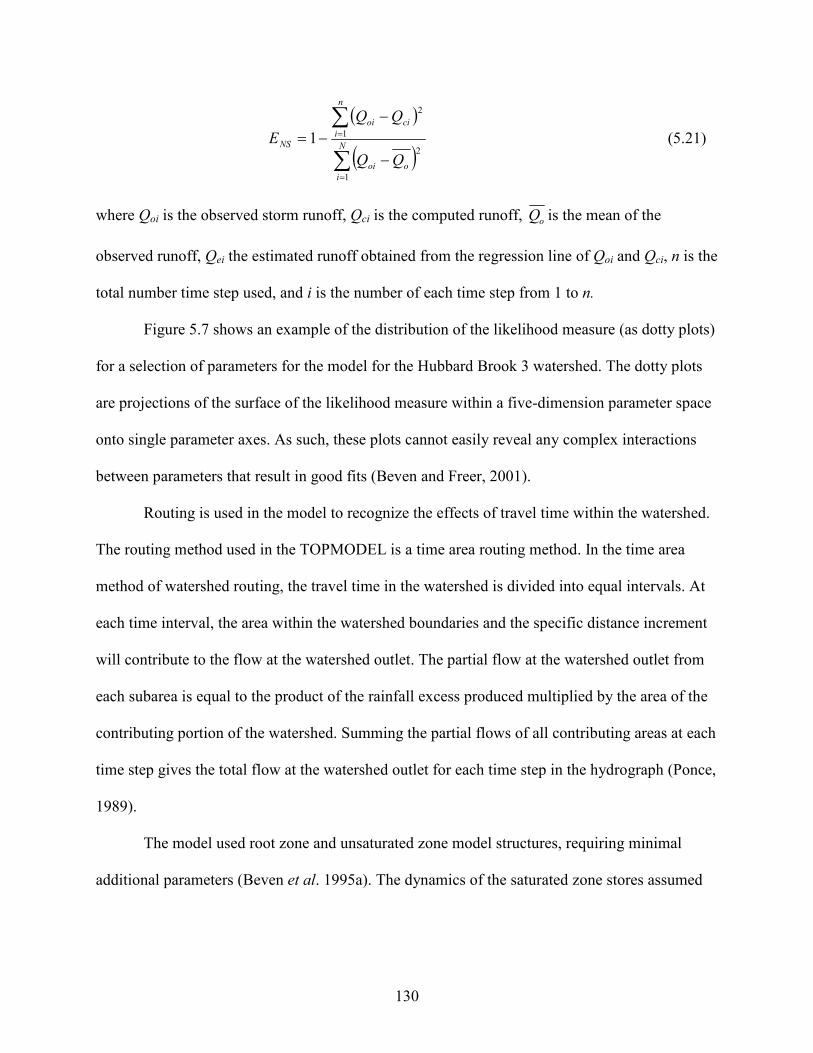
130

( )

( )∑

∑

=

=

−

−−=

N

i

ooi

n

i

cioi

NS

QQ

QQ

E

1

2

1

2

1 (5.21)

where Qoi is the observed storm runoff, Qci is the computed runoff, oQ is the mean of the

observed runoff, Qei the estimated runoff obtained from the regression line of Qoi and Qci, n is the

total number time step used, and i is the number of each time step from 1 to n.

Figure 5.7 shows an example of the distribution of the likelihood measure (as dotty plots)

for a selection of parameters for the model for the Hubbard Brook 3 watershed. The dotty plots

are projections of the surface of the likelihood measure within a five-dimension parameter space

onto single parameter axes. As such, these plots cannot easily reveal any complex interactions

between parameters that result in good fits (Beven and Freer, 2001).

Routing is used in the model to recognize the effects of travel time within the watershed.

The routing method used in the TOPMODEL is a time area routing method. In the time area

method of watershed routing, the travel time in the watershed is divided into equal intervals. At

each time interval, the area within the watershed boundaries and the specific distance increment

will contribute to the flow at the watershed outlet. The partial flow at the watershed outlet from

each subarea is equal to the product of the rainfall excess produced multiplied by the area of the

contributing portion of the watershed. Summing the partial flows of all contributing areas at each

time step gives the total flow at the watershed outlet for each time step in the hydrograph (Ponce,

1989).

The model used root zone and unsaturated zone model structures, requiring minimal

additional parameters (Beven et al. 1995a). The dynamics of the saturated zone stores assumed

131

an exponential decline in conductivity with depth. Table 5.2 lists parameters required for the

model and the ranges assigned to each for the Monte Carlo simulations.

Results and discussion

A topographic index values are determined for all grid cells using GRIDATB (a multiple

flow direction algorithm) for each watersheds. The distribution of the topographic index values

for all watersheds is illustrated in Figure 5.8 (fractional area, As /A versus Topographic index

values). Higher values of the topographic index indicate higher potential of the landscape to

generate runoff to become wet. The average values of the topographic index, λ, (see Equation

5.7) are 5.86, 5.13, 4.65, and 6.36 for Coweeta 2, Coweeta36, Fernow 4, and Hubbard Brook 3,

respectively (Table 5.3). Fernow 4 has the lowest (0.81) and the highest (13.88) topographic

index values. The high topographic index band widened from the upstream side of the streams

down towards the watershed outlet (Figure 5.8). The low topographic index classes are

associated with the upland areas, which did not contribute directly to runoff. In all cases, the

map (Figure 5.8) showed a trend of increasing topographic index values from the escarpment to

around the lower stream channel areas, indicating that the runoff-contributing areas were largely

located along the stream channel of the watersheds.

The top ranked parameter sets, out of the 10,000 randomly selected parameter sets run for

the first three storm events, used to select parameter sets having the same values for all events.

This procedure was repeated for all watersheds during the calibration process. The selected

parameter sets are tested assigning the same values of parameter sets and run the model for the

remaining three storm events. The range of the parameters used together with the efficiency of

the model during the calibration and testing procedures is given in Table 5.7.

132

Figure 5.7 shows the scatter plots of maximum likelihood versus parameter values. All

values with negative efficiency are excluded from the plots. The scatter plots show the

exponential transmissivity function or recession curve parameter (m) is the most sensitive to

model performance for all watersheds compared to the other parameters. The scatter plot had a

peaked band of dots, which meant that the best model performances occurred for parameter sets,

for example, having m values between 0.008 and 0.016 meter for Hubbard Brook watershed 3.

The scatter plot of the initial storage deficit in the root zone parameter (SRinit) indicated a

tendency of achieving better results between 0.0 and 0.01 meter, but high modeling efficiencies

are also obtained from values as high as 0.02 meter. The scatter plot of the soil profile storage

available for transpiration, i.e. an available water capacity (SRmax), the natural logarithm of the

effective transmissivity of the soil when just saturated (ln To) and an effective surface routing

velocity (ChVel) parameters were completely flat topped across the range of parameter values set.

In general, the scatter plots indicated a high degree of equifinality between parameter sets,

meaning that wide ranges of parameter values were included in the parameter sets (Beven 2000).

The simulated hydrograph during the calibrating and testing procedures compared well

with the observed hydrograph for Hubbard Brook 3 and Fernow 4 watersheds. The timing, shape

and magnitude of the simulated hydrograph during the, rising, peak, and recession periods of

each storm events was very well reproduced by the model (Figures 5.10 and 5.11). The Nash

Sutcliffe efficiency during the calibration and testing procedures are 93.4 percent and 87.9

percent for Fernow 4 and 91.0 percent and 82.7 percent for Hubbard Brook 3 (Table 5.7). All

hydrographs generated in the TOPMODEL are in units of m/time step used or (m3/time step/m2)

and the results are shown in the same units. The Coweeta 36 showed relatively poor performance

(calibrating and testing Nash Sutcliffe efficiency of 76.9 percent and 70.3 percent) compared to

133

Fernow 4 and Hubbard Brook 3 watersheds (Table 5.7 and Figure 5.9). The TOPMODEL failed

to simulate runoff for the selected storm events of Coweeta 2 watershed. During the calibration

procedure, the same values of parameter sets were not obtained for Coweeta 2. This means a

single set of parameter would not provide a good fit to the observed runoff. In most of the storm

events, the top ranked parameter sets, out of the 10,000 randomly selected parameter sets failed

to provide a good performance of the model. The unique watershed characteristic of Coweeta 2

is that the watershed has greater soil depth compared to the other watershed. The other reason

could be the shape of the watershed has longer length and narrower width compared to rest of the

watersheds. Probably, this is the reason that the model does not perform well for Coweeta 2

watershed.

Conclusions

Tests of TOPMODEL calibrations for three single rainfall events on four small, forested

watersheds showed very good hydrograph simulations for three drainages. The calibrations for

watersheds produced a common parameter set for all three, calibration rainfall events on each

drainage. Coweeta 2 required different parameter sets for each of the three calibration storms.

The deeper soil of Coweeta 2 is perhaps the reason for the poor performance.

Acknowledgments

Financial assistance provided in part by funds from The U.S. Geological Survey through

the Georgia institute of Water Resources, and Warnell School of Forest and Natural Resources.

Professor K. J. Beven from Lancaster University, UK is gratefully acknowledged for providing

initial guidance and comments on this study. The watershed characteristics, rainfall, and runoff

134

datasets required for the study are provided by Wayne Swank and Stephanie from the Coweeta

Hydrologic Laboratory; Frederica Wood, from the Fernow Timber and Watershed Laboratory;

and John Campbell, from the Hubbard Brook Experimental Forest.

References

Beven, K. J. 1996. A discussion of distributed modeling. In Distributed Hydrological Modeling,

Abbott, M. B. and J. C. Refsgaard, eds. Kluwer, Dordrecht, pp. 255-278.

Beven, K. J. 1997. TOPMODEL: a critique. Hydrological Processes 11(9): 1069-1085. doi:

10.1002/(SICI)1099-1085(199707)11:9<1069::AID-HYP545>3.0.CO;2-O.

Beven, K. J. 2000. Rainfall-runoff modeling: The primer. John Willey and Sons, New York,

New York.

Beven, K. J. and J. Freer. 2001. A dynamic TOPMODEL. Hydrological Processes 15(10): 1993-

2011. DOI: 10.1002/hyp.252.

Beven K. J. and Kirkby, M. J. 1979. A physically-based variable contributing area model of

basin hydrology. Hydrological Sciences Journal 24: 43–69

Beven, K. J., R. Lamb, P. F. Quinn, R. Romanowicz, J. Freer. 1995a. TOPMODEL. In Computer

Models of Watershed Hydrology, V. P. Singh, ed. Water Resources Publications,

Highlands Ranch, Colorado, 627–668.

Beven, K. J., P. F. Quinn, R. Romanowicz, J. Freer, J. Fisher, and R. Lamb, 1995b. TOPMODEL

AND GRIDATB: A Users Guide to the Distributed Versions (95.02). CRES Technical

Report TR110, 2nd Ed. Center for Research on Environmental Systems and Statistics,

Institute of Environmental and Biological Sciences, Lancaster, United Kingdom.

135

Bhaskar, N. R., L. K. Brummett, and M. N. French. 2005. Runoff modeling of a mountainous

catchment using TOPMODEL: A case study. Journal of the American Water Resources

Association 41(1): 107-121.

Boughton, W. C. 1987. Evaluating partial areas of watershed runoff. Journal of Irrigation and

Drainage Engineering 113(3): 356-366.

Campling, P., A. Gobin, K. Beven, and J. Feyen. 2002. Rainfall-runoff modeling of a humid

tropical catchment: the TOPMODEL approach. Hydrological Processes 16(2): 231–253.

doi: 10.1002/hyp.341.

Dunne T, and R. D. Black, 1970. Partial area contributions to storm runoff in a small New

England watershed. Water Resources Research 6(2): 478–490.

Dunne, T., T. R. Moore, and C. H. Taylor. 1975. Recognition and prediction of runoff-producing

zones in humid regions. Hydrological Sciences Bulletin 20(3): 305-327.

Garbrecht, J., F. Ogden, P. A. Barry, and D. R. Maidment. 2001. GIS and distributed watershed

models 1. Data coverages and sources. Journal of Hydrologic Engineering 6(6): 506-514.

Hewlett, J. D. and A. R. Hibbert. 1967. Factors affecting response of small watersheds to

precipitation in humid areas. In International Symposium on Forest Hydrology, W. B.

Sopper and H. W. Lull, ed. Proceedings of a National Science Foundation Advanced

Science Seminar. August 29 to September 10, 1965, Pennsylvania State University,

University Park, Pennsylvania, Pergamon Press, New York, New York, 275-290.

Kirkby, M. J. and D. R. Weyman. 1974. Measurements of contributing areas in very small

drainage basins. Seminar Series B, No. 3, Department of Geography, University of

Bristol, Bristol, United Kingdom.

136

Lyon, S. W., M. T. Walter, P. G´erard-Marchant, and T. S. Steenhuis. 2004. Using a topographic

index to distribute variable source area runoff predicted with the SCS curve-number

equation, Hydrological Processes 18: 2757–2771.

McCutcheon, S. C., Tedela N. H., Adams, M. B., Swank, W., Campbell, J. L., Hawkins, R. H.,

Dye, C. R. 2006. Rainfall-runoff relationships for selected eastern U.S. forested mountain

watersheds: Testing of the curve number method for flood analysis. Report prepared for

the West Virginia Division of Forestry, Charleston, West Virginia.

Nachabe, M. H. 2006. Equivalence between TOPMODEL and the NRCS curve number method

in predicting variable runoff source areas. Journal of the American Water Resources

Association 42(1): 225-235.

Nash, J. E. and J. V. Sutcliffe. 1970. River flow forecasting through conceptual models part I-A.

discussion of principles. Journal of Hydrology 10(3): 282-290.

Pierce, R. S. 1967. Evidence of overland flow on forest watersheds. In: International Symposium

on Forest Hydrology W. E. Sopper and H. W. Lull, eds. Proceedings of a National

Science Foundation Advanced Science Seminar, Pergamon Press, New York, New York,

247–253.

Ponce, V. M. 1989. Engineering Hydrology. Prentice-Hall, Inc., Englewood Cliffs, New Jersey,

640 pp.

Quinn, P. F., K. J. Beven, and R. Lamb. 1995. The ln (a/tan β) index: How to calculate it and

how to use it in the TOPMODEL framework. Hydrological Processes 2(9): 161-182.

Rallison, R. E. 1980. Origin and evolution of the SCS runoff equation. In Proceedings of the

Symposium on Watershed Management, American Society of Civil Engineers, New

York, New York, 912-924.

137

Reinhart, K. G., A. R. Eschner, and G. R. Tremble, Jr. 1963. Effect on streamflow of four forest

practices. U.S. Department of Agriculture Forest Service Research Paper NE-1,

Northeastern Forest Experiment Station, Upper Darby, Pennsylvania.

Robson A. J., P. G. Whitehead, and R. C. Johnson. 1993. An application of a physically based

semi-distributed model to the Balquhidder catchments. Journal of Hydrology 145(3-4):

357–370.

Steenhuis, T. S., M. Winchell, J. Rossing, J. A. Zollweg, and M. F. Walter. 1995. SCS runoff

equation revisited for variable-source runoff areas. Journal of Irrigation and Drainage

Engineering 121(3): 234-238.

Troendle, C. A. 1970b. The flow interval method for analyzing timber harvesting effects on

streamflow regimen. Water Resources Research 6(1): 328-332.

U.S. Department of Agriculture (USDA). 2004. Experimental forests and ranges of the USDA

Forest Service, General Technical Report NE-321, Northern Research Station, Newtown

Square, Pennsylvania, 178 pp.

138

Table 5.1 Characteristics of four mountainous forested watersheds in the eastern United States

Watershed Area

(hectares) Dominant aspect

Elevation

range

(meters)

Channel

length

(meters)

Average

slope

(%)

Annual

precipitation

(millimeter)

Coweeta 2 12.3 South by southeast 709 - 1004 392 60.2 1812

Coweeta 36 46.6 East by southeast 1021 - 1542 1327 65.3 2015

Fernow 4 38.7 East by southeast 740 - 865 683 20.6 1450

Hubbard Brook 3 42.4 Southwest 527 - 732 961 27.5 1370

139

Table 5.2 Parameter ranges

Parameters Symbol Units Range

Exponential transmissivity function m [L] 0.005 - 0.05

The natural logarithm of the effective transmissivity of the soil LnTo [L2T-1] 1.0 - 10.0

Soil profile storage available for transpiration SRmax [L] 0.01 - 1.0

Initial storage deficit in the root zone SRinit [L] 0.0 - 1.0

Channel velocity ChVel [LT-1] 1000 - 5000

140

Table 5.3 Range of topographic index values for all watersheds

Values of Topographic Index

Watershed Smallest Largest

Fractional area weighted average

Coweeta 2 2.68 12.12 5.86

Coweeta 36 2.26 13.00 5.13

Fernow 4 0.81 13.88 4.65

Hubbard Brook 3 2.70 13.87 6.36

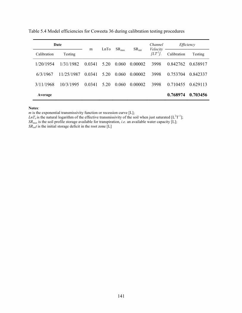
141

Table 5.4 Model efficiencies for Coweeta 36 during calibration testing procedures

Date Efficiency

Calibration Testing m LnTo SRmax SRinit

Channel

Velocity

[LT-1]. Calibration Testing

1/20/1954 1/31/1982 0.0341 5.20 0.060 0.00002 3998 0.842762 0.638917

6/3/1967 11/25/1987 0.0341 5.20 0.060 0.00002 3998 0.753704 0.842337

3/11/1968 10/3/1995 0.0341 5.20 0.060 0.00002 3998 0.710455 0.629113

Average 0.768974 0.703456

Notes: m is the exponential transmissivity function or recession curve [L]; LnTo is the natural logarithm of the effective transmissivity of the soil when just saturated [L2T-1]; SRmax is the soil profile storage available for transpiration, i.e. an available water capacity [L]; SRinit is the initial storage deficit in the root zone [L]

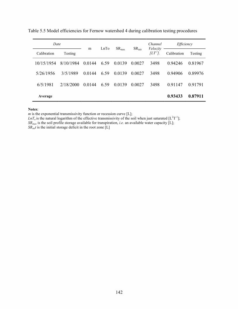
142

Table 5.5 Model efficiencies for Fernow watershed 4 during calibration testing procedures

Date Efficiency

Calibration Testing m LnTo SRmax SRinit

Channel

Velocity

[LT-1]. Calibration Testing

10/15/1954 8/10/1984 0.0144 6.59 0.0139 0.0027 3498 0.94246 0.81967

5/26/1956 3/5/1989 0.0144 6.59 0.0139 0.0027 3498 0.94906 0.89976

6/5/1981 2/18/2000 0.0144 6.59 0.0139 0.0027 3498 0.91147 0.91791

Average 0.93433 0.87911

Notes: m is the exponential transmissivity function or recession curve [L]; LnTo is the natural logarithm of the effective transmissivity of the soil when just saturated [L2T-1]; SRmax is the soil profile storage available for transpiration, i.e. an available water capacity [L]; SRinit is the initial storage deficit in the root zone [L]

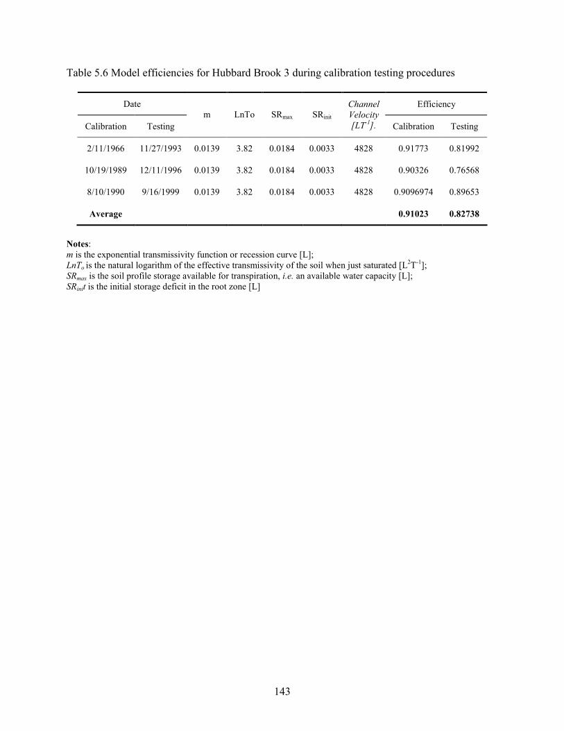
143

Table 5.6 Model efficiencies for Hubbard Brook 3 during calibration testing procedures

Date Efficiency

Calibration Testing m LnTo SRmax SRinit

Channel

Velocity

[LT-1]. Calibration Testing

2/11/1966 11/27/1993 0.0139 3.82 0.0184 0.0033 4828 0.91773 0.81992

10/19/1989 12/11/1996 0.0139 3.82 0.0184 0.0033 4828 0.90326 0.76568

8/10/1990 9/16/1999 0.0139 3.82 0.0184 0.0033 4828 0.9096974 0.89653

Average 0.91023 0.82738

Notes: m is the exponential transmissivity function or recession curve [L]; LnTo is the natural logarithm of the effective transmissivity of the soil when just saturated [L2T-1]; SRmax is the soil profile storage available for transpiration, i.e. an available water capacity [L]; SRinit is the initial storage deficit in the root zone [L]

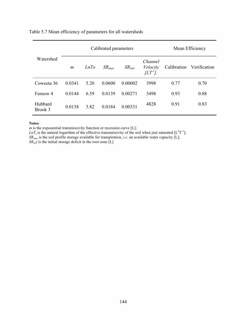
144

Table 5.7 Mean efficiency of parameters for all watersheds

Calibrated parameters Mean Efficiency

Watershed

m LnTo SRmax SRinit

Channel

Velocity

[LT-1].

Calibration Verification

Coweeta 36 0.0341 5.20 0.0600 0.00002 3998 0.77 0.70

Fernow 4 0.0144 6.59 0.0139 0.00271 3498 0.93 0.88

Hubbard Brook 3

0.0138 3.82 0.0184 0.00331 4828 0.91 0.83

Notes: m is the exponential transmissivity function or recession curve [L]; LnTo is the natural logarithm of the effective transmissivity of the soil when just saturated [L2T-1]; SRmax is the soil profile storage available for transpiration, i.e. an available water capacity [L]; SRinit is the initial storage deficit in the root zone [L]

145

Figure 5.1 Location of study watersheds

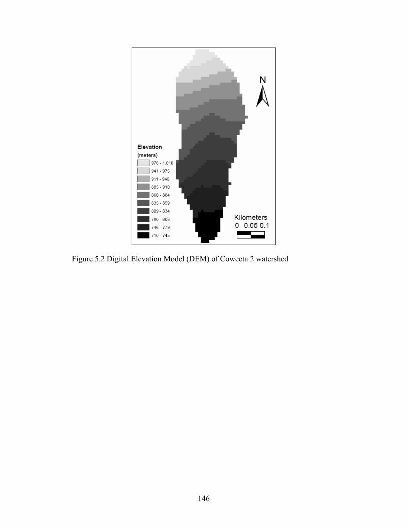
146

Figure 5.2 Digital Elevation Model (DEM) of Coweeta 2 watershed

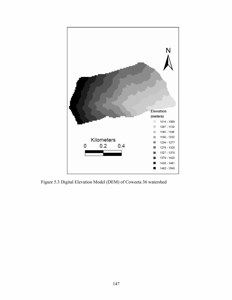
147

Figure 5.3 Digital Elevation Model (DEM) of Coweeta 36 watershed

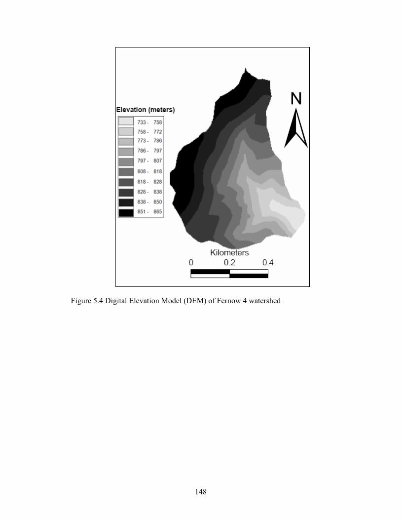
148

Figure 5.4 Digital Elevation Model (DEM) of Fernow 4 watershed

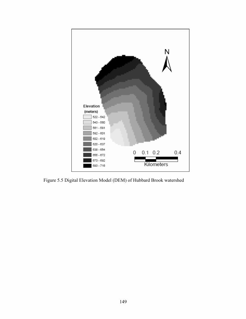
149

Figure 5.5 Digital Elevation Model (DEM) of Hubbard Brook watershed

150

.

0.00

0.02

0.04

0.06

0.08

3 4 5 6 7 8 9 11 12

Topographic Index

Histogram of fractional area (As/A)

Coweeta 2

As = Saturated area

A = Total area

0.0

0.2

0.4

0.6

0.8

1.0

2 3 4 5 6 7 8 9 10 11 12

Topographic Index

Commutative farctional area (As/A)

Coweeta 2

As = Saturated area

A = Total area

0.00

0.02

0.04

0.06

0.08

0.10

0.12

2 4 5 6 7 9 10 11 13

Topographic Index

Histogram of fractional area (As/A)

Coweeta 36

As = Saturated area

A = Total area

0.0

0.2

0.4

0.6

0.8

1.0

0 2 4 6 8 10 12 14

Topographic Index

Commutative fractional area (As/A)

Coweeta 36

As = Saturated area

A = Total area

0.00

0.02

0.04

0.06

0.08

0.10

0.12

1 2 3 4 5 6 7 8 9 10 11 12 13

Topographic Index

Histogram of fractional area (As/A)

Fernow 4

As = Saturated area

A = Total area

0.0

0.2

0.4

0.6

0.8

1.0

0 2 4 6 8 10 12 14 16

Topographic Index

Commutative fractional area (As/A)

Fernow 4

As = Saturated area

A = Total area

0.00

0.02

0.04

0.06

0.08

0.10

3 4 5 6 7 8 9 11 12 13 14

Topographic Index

Histogram of fractional area (As/A)

Hubbard Brook 3

As = Saturated area

A = Total area

0.0

0.2

0.4

0.6

0.8

1.0

0 2 4 6 8 10 12 14 16

Topographic Index

Cumulative fractional area (As/A)

Hubbard Brook 3

As = Saturated area

A = Total area

Figure 5.6 Distribution of topographic index for all watersheds

151

0

0.2

0.4

0.6

0.8

1

0.00 0.01 0.02 0.03 0.04 0.05 0.06

Exponential transmissivity function (m )

Efficiency (ENS)

Range = 0.005 - 0.05

0

0.2

0.4

0.6

0.8

1

0 2 4 6 8 10 12

Natural logatithm of the effective transmissivity

of the soil when saturated (lnT o )

Efficiency (ENS)

Range = 1 -10

0

0.2

0.4

0.6

0.8

1

0.00 0.02 0.04 0.06 0.08 0.10 0.12

Available water capacity (SR max )

Efficiency (E

NS)

Range = 0.01 - 1.0

0

0.2

0.4

0.6

0.8

1

0 0.01 0.02 0.03 0.04 0.05 0.06

Initial storage deficit in the root zone (SR int )

Efficiency (ENS)

Range = 0 - 1

0

0.2

0.4

0.6

0.8

1

0 1000 2000 3000 4000 5000 6000

Surface routing velocity (Ch Vel )

Efficiency (ENS)

Range = 1000 - 5000

Figure 5.7 Dotty plots for all parameters for the Hubbard Brook watershed 3. Each dot represents one simulation with different randomly chosen parameter values within the ranges as shown in Table 5.2.

152

(a) Coweeta 2

(c) Fernow 4

(b) Coweeta 36

(d) Hubbard Brook 3

Figure 5.8.The spatial pattern of the topographic index classes used in the TOPMODEL as determined from an analysis of surface topography.

153

Figure 5.9 Comparison of observed and simulated hydrograph for Hubbard Brook watershed 3 [(a) Calibration and (b) Testing]

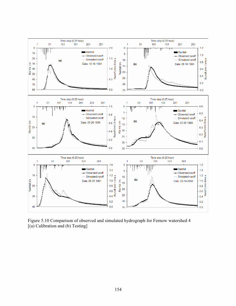
154

Figure 5.10 Comparison of observed and simulated hydrograph for Fernow watershed 4 [(a) Calibration and (b) Testing]

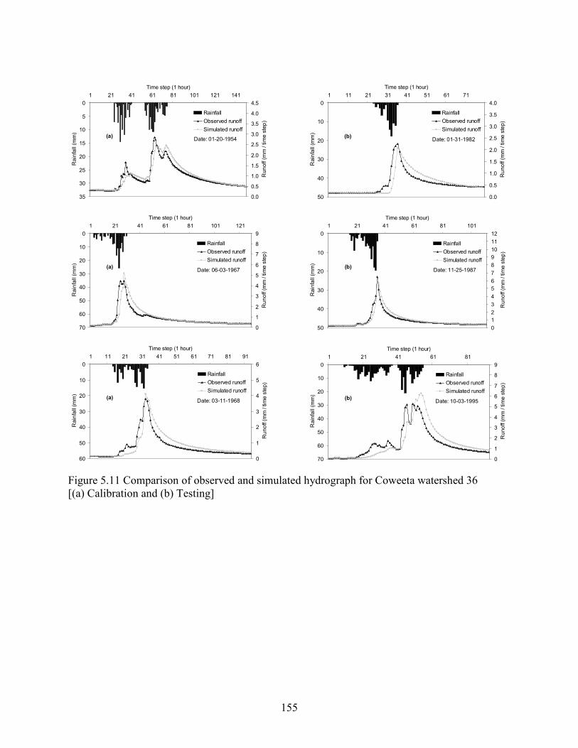
155

0

5

10

15

20

25

30

35

1 21 41 61 81 101 121 141

Time step (1 hour)

Rainfall (mm)

0.0

0.5

1.0

1.5

2.0

2.5

3.0

3.5

4.0

4.5

Runoff (mm / tim

e step)

Rainfall

Observed runoff

Simulated runoff

Date: 01-20-1954(a)

0

10

20

30

40

50

60

70

1 21 41 61 81 101 121

Time step (1 hour)

Rainfall (mm)

0

1

2

3

4

5

6

7

8

9

Runoff (mm / tim

e step)

Rainfall

Observed runoff

Simulated runoff

Date: 06-03-1967(a)

0

10

20

30

40

50

60

1 11 21 31 41 51 61 71 81 91

Time step (1 hour)

Rainfall (mm)

0

1

2

3

4

5

6

Runoff (mm / tim

e step)

Rainfall

Observed runoff

Simulated runoff

Date: 03-11-1968(a)

0

10

20

30

40

50

1 11 21 31 41 51 61 71

Time step (1 hour)

Rainfall (mm)

0.0

0.5

1.0

1.5

2.0

2.5

3.0

3.5

4.0

Runoff (mm / tim

e step)

Rainfall

Observed runoff

Simulated runoff

Date: 01-31-1982(b)

0

10

20

30

40

50

1 21 41 61 81 101

Time step (1 hour)

Rainfall (mm)

0

1

2

3

4

5

6

7

8

9

10

11

12

Runoff (mm / tim

e step)

Rainfall

Observed runoff

Simulated runoff

Date: 11-25-1987(b)

0

10

20

30

40

50

60

70

1 21 41 61 81

Time step (1 hour)

Rainfall (mm)

0

1

2

3

4

5

6

7

8

9

Runoff (mm / tim

e step)

Rainfall

Observed runoff

Simulated runoff

Date: 10-03-1995(b)

Figure 5.11 Comparison of observed and simulated hydrograph for Coweeta watershed 36 [(a) Calibration and (b) Testing]

156

CHAPTER 6

CONCLUSIONS

The Natural Resources Conservation Service (2001) tabulated curve numbers based on

soil hydrologic group, land use, and surface condition were not adequate to estimate runoff for

the ten small, mountainous-forested watersheds in the eastern United States. All runoff values

estimated from Natural Resources Conservation Service tabulated curve numbers were

significantly biased. Therefore, the current Natural Resources Conservation Service (2001)

tabulations for “woods” should not be used to estimate runoff in forested watersheds unless the

estimated curve numbers are independently confirmed using calibration data from gaged

watersheds with similar hydrologic conditions.

The curve numbers determined from annual maximum series of observed rainfall and

runoff indicate wide variability from average runoff conditions for a particular watershed and,

hence, a unique curve number does not provide an adequate estimate of runoff volume. Observed

and estimated runoff volumes were not highly correlated for six of ten-forested watersheds.

Therefore, the calibrated curve numbers for gauged, forested watersheds also contain large

uncertainties, and should only be used if statistical analyses confirm that estimated runoff

adequately agrees with observations.

No significant difference (at the 0.05 level of significance) exists in using either of the

median, geometric mean, or arithmetic mean curve number (computed from measured rainfall

and runoff events) to estimate runoff for all watersheds. However, for some watersheds the

157

estimates based on any of the central tendency based curve number did not agree with

measurements. .

The growing-season curve numbers were significantly different from that of the dormant

season curve numbers for only three of the six gaged watersheds. The lack of statistical evidence

of seasonal effects was apparently due to the large uncertainties in curve numbers

Paired studies on three watersheds suggested that timber harvesting increased streamflow

and, hence, increased curve numbers derived from observed rainfall and runoff data. However,

the increase in curve number was not significant (at the 0.05 level of significance) for one of

three clearcuts

The probability distributions of three watersheds (out of four watersheds) demonstrated

that the Natural Resources Conservation Service tabulated curve number method estimated

runoff for extreme rainfall events, occurring once in one hundred years or longer. This means,

the tabulated curve number may predict runoff for events occurring rarely and under predicts

runoff for less frequent rainfall events. In general, the four discrete distributions of estimated

runoff only crossed the discrete observed runoff distribution a single point or short interval and

these points or intervals did not consistently correspond to the two-year return intervals for the

which the tabulated curve numbers were developed. The limited intersections at different return

intervals also imply that single watershed curve numbers for these four watersheds may not be

adequate. The gamma distribution matched the observed annual maximum rainfall and runoff for

all watersheds.

The TOPMODEL provides a better prediction of runoff for three of the four watersheds

considered. However, the model failed to simulate runoff accurately for one of (Coweeta 2) the

158

watersheds at an acceptable efficiency. The TOPMODEL could only be calibrated for Coweeta 2

with three different sets of parameters for the three rainfall events selected for calibration.

159

REFERENCES

Abbott, M. B., J. C. Bathurst, J. A. Cunge, P. E. O’Connell, and J. L. Rasmussen. 1986. An

introduction to the European Hydrology System SHE, 2, Structure of a physically-based,

distributed modeling system. Journal Hydrology 87(1-2): 61-77.

Aitkin, A. S. 1973. Assessing systematic errors in rainfall-runoff models. Journal of Hydrology

20(2): 121-136.

Anderson, T. W. 1962. On the distribution of the two-sample Cramer-von Mises criterion.

Annals of Mathematical Statistics 33(3): 1148-1159.

Andrews, R. G. 1954. The use of relative infiltration indices in computing runoff. Soil

Conservation Service, Forth Worth, Texas. (unpublished).

Arnold, J. G., J. R. Williams, R. H. Griggs, and N. B. Sammons. 1990. SWRRB–A basin scale

simulation model for soil and water resources management. Texas A&M Press, College

Station, Texas.

Arnold, J. G., P. M. Allen, and G. Bernhardt. 1993. A comprehensive surface–groundwater flow

model. Journal of Hydrology 142(1-4): 47-69.

Bathurst, J. C. 1986. Sensitivity analysis of the Systéme Hydrologique Europeén for an upland

catchment. Journal of Hydrology 87(1-2): 103-123.

Beck, M. B. 1991. Forecasting environmental change. Journal of Forecasting 10(1-2): 3-19. doi:

10.1002/for.3980100103.

160

Bedient, P. B. and W. C. Huber. 1992. Hydrology and Floodplain Analysis. Addison and

Wesley, New York, New York.

Bergström, S. 1995. The HBV model. In Computer Models of Watershed Hydrology, V. P.

Singh, ed. Water Resource Publication, Highlands Ranch, Colorado.

Beven, K. J. 1983. Surface water hydrology-runoff generation and basin structure. Reviews of

Geophysics 21(3): 721-730.

Beven, K. J. 1989. Changing ideas in hydrology: The case of physically-based models. Journal

of Hydrology 105(1-2): 157–172.

Beven, K. J. 1996. A discussion of distributed modeling. In Distributed Hydrological Modeling,

Abbott, M. B. and J. C. Refsgaard, eds. Kluwer, Dordrecht, pp. 255-278.

Beven, K. J. 1997. TOPMODEL: a critique. Hydrological Processes 11(9): 1069-1085. doi:

10.1002/(SICI)1099-1085(199707)11:9<1069::AID-HYP545>3.0.CO;2-O.

Beven, K. J. 2000. Rainfall-runoff modeling: The primer. John Willey and Sons, New York,

New York.

Beven, K. J. and J. Freer. 2001. A dynamic TOPMODEL. Hydrological Processes 15(10): 1993-

2011. DOI: 10.1002/hyp.252.

Beven, K. J. and M. J. Kirkby. 1979. A physically-based, variable contributing area model of

basin hydrology. Hydrological Sciences Journal 24: 43-69.

Beven, K. J., A. Calver, and E. M. Morris. 1987. The Institute of Hydrology distributed model.

Technical Report 89, Institute of Hydrology, Wallingford, United Kingdom.

Beven, K. J., R. Lamb, P. F. Quinn, R. Romanowicz, J. Freer. 1995a. TOPMODEL. In Computer

Models of Watershed Hydrology, V. P. Singh, ed. Water Resources Publications,

Highlands Ranch, Colorado, 627–668.

161

Beven, K. J., P. F. Quinn, R. Romanowicz, J. Freer, J. Fisher, and R. Lamb, 1995b. TOPMODEL

and GRIDATB: A Users Guide to the Distributed Versions (95.02). CRES Technical

Report TR110, 2nd Ed. Center for Research on Environmental Systems and Statistics,

Institute of Environmental and Biological Sciences, Lancaster, United Kingdom.

Bhaskar, N. R., L. K. Brummett, and M. N. French. 2005. Runoff modeling of a mountainous

catchment using TOPMODEL: A case study. Journal of the American Water Resources

Association 41(1): 107-121.

Binley, A. M., and K. J. Beven. 1989. A physically based model of heterogeneous hillslopes 2.

Effective hydraulic conductivities. Water Resources Research 25(6): 1227-1233.

Blom, G. 1958. Statistical Estimates and Transformed Beta Variables. Wiley, New York, New

York.

Bonell, M. and J. Williams. 1986. The generation and redistribution of overland flow on a

massive oxic soil in eucalypt woodland within the semi-arid tropics of north Australia.

Hydrological Processes 1(1): 31-46.

Boughton, W. C. 1984. A simple model for estimating the water yield of ungauged catchments.

Civil Engineering Transactions 26(2): 83–88.

Boughton, W. C. 1987. Evaluating partial areas of watershed runoff. Journal of Irrigation and

Drainage Engineering 113(3): 356-366.

Bras, R. L. 1990. Hydrology: An Introduction to Hydrologic Science. Addison and Wesley, New

York.

Campling, P., A. Gobin, K. Beven, and J. Feyen. 2002. Rainfall-runoff modeling of a humid

tropical catchment: the TOPMODEL approach. Hydrological Processes 16(2): 231–253.

doi: 10.1002/hyp.341.

162

Chakravarti, I. M., R. G. Laha, and J. Roy. 1967. Handbook of Methods of Applied Statistics,

Volume I. John Wiley and Sons, 392-394.

Chiew, F. and T. McMahon. 1994. Application of the daily rainfall runoff model

MODHYDROLOG to 28 Australian catchments. Journal of Hydrology 153(1-4): 383-

416.

Chin, D. A. 2006. Water Resources Engineering. 2nd Ed. Prentice Hall, Upper Saddle River, New

Jersey.

Chorley, R. J. 1978. The hillslope hydrological cycle. In Hillslope Hydrology, M. J. Kirkby, ed.

John Wiley and Sons, New York, New York, 1–42.

Chow, V. T., ed. 1964. Handbook of Applied Hydrology. McGraw-Hill, New York, New York.

Crawford, N. H. and R. K. Linsley. 1966. Digital simulation in hydrology. Stanford Watershed

Model IV. Department of Civil Engineering Report 39, Stanford University, Stanford,

California.

Cunnane, C. 1978. Unbiased plotting position - a review. Journal of Hydrology 37(3-4): 205-

222. doi:10.1016/0022-1694(78)90017-3.

De Michele, C. and G. Salvadori. 2002. On the derived flood frequency distribution: Analytical

formulation and the influence of antecedent soil moisture condition. Journal of

Hydrology 262(1-4): 245-258.

Dunne T, and R. D. Black, 1970. Partial area contributions to storm runoff in a small New

England watershed. Water Resources Research 6(2): 478–490.

Dunne, T. and L. Leopold. 1978. Water in Environmental Planning. Freeman and Company,

New York, New York.

163

Dunne, T., T. R. Moore, and C. H. Taylor. 1975. Recognition and prediction of runoff-producing

zones in humid regions. Hydrological Sciences Bulletin 20(3): 305-327.

Freer, J., K. Beven, and B. Ambroise. 1996. Bayesian estimation of uncertainty in runoff

prediction and the value of data: an application of the GLUE approach. Water Resources

Research 32(7): 2161–2173.

Freeze, R. A. 1972. Role of subsurface flow in generating surface runoff 2. upstream source

areas. Water Resources Research 8(5): 1272-1283.

Freeze, R. A. 1980. A stochastic–conceptual analysis of rainfall-runoff processes on a hillslope.

Water Resources Research 16(2): 391–408.

Freeze, R. A. and J. Cherry. 1979. Groundwater. Prentice-Hall, Inc., Englewood Cliffs, New

Jersey.

Garbrecht, J. and L. Martz. 1994. Grid size dependency of parameters extracted from digital

elevation models. Computers and Geosciences 20(1): 85-87.

Garbrecht, J., F. Ogden, P. A. Barry, and D. R. Maidment. 2001. GIS and distributed watershed

models 1. Data coverages and sources. Journal of Hydrologic Engineering 6(6): 506-514.

Garen, D. C. and D. S. Moore. 2005. Curve number hydrology in water quality modeling: uses,

abuses, and future directions. Journal of the American Water Resources Association

41(2): 377-388.

Goudie, A. 1990. The Human Impact on the Natural Environment. 3rd Ed. The MIT Press

Cambridge, Massachusetts.

Grayson, R. B., I. D. Moore, and T. A. McMahon. 1992. Physically based hydrologic modeling

2. Is the concept realistic? Water Resources Research 28(10): 2659-2666.

164

Gringorten, I. I. 1963. A plotting rule for extreme probability paper. Journal of Geophysical

Research 68(3) 813-814.

Haan, C. T. 2002. Statistical Methods in Hydrology. Iowa State University Press, Ames.

Haith, D. A. and L. L. Shoemaker. 1987. Generalized watershed loading functions for stream-

flow nutrients. Water Resources Research 23(3): 471–478.

Hammer, M. J. and K. A. MacKichan. 1981. Hydrology and Quality of Water Resources. Wiley,

New York, New York.

Harbor, J. M. 1994. Practical method for estimating the impact of land-use change on surface

runoff, Groundwater Recharge and Wetland Hydrology , Journal of the American

Planning Association 60(1): 95-108.

Hawkins, R. H. 1993. Asymptotic determination of runoff curve numbers from data. Journal of

Irrigation and Drainage Engineering 119(2): 334-345.

Hawkins, R. H. 1998. Local sources for runoff curve numbers. Eleventh Annual Symposium of

the Arizona Hydrological Society, September 23-26, Tucson, Arizona.

Hawkins, R. H., E. D. Woodward, J. Ruiyun, J. E. VanMullem, and A. T. Hjelmfelt. 2005.

Runoff Curve Number method: examination of the initial abstraction ratio. ASCE

Watershed Management CN Workshop, Williamsburg, Virginia, originally given at the

Federal Interagency Hydrologic Modeling Conference, July 2002, Las Vegas, Nevada.

Hawkins, R. H., University of Arizona, Tucson, Personal communication, 2006.

Hazen, A. 1914. Storage to be provided in impounding reservoirs for municipal water supply.

Transaction of the American Society of Civil Engineers paper 1308, 77: 1547-1550. (from

Cunnane, 1978).

165

Helweg, O. J. 1991. Microcomputers Applications in Water Resources. Prentice Hall, Inc.,

Englewood Cliffs, New Jersey.

Hewlett, J. D. and A. R. Hibbert. 1967. Factors affecting response of small watersheds to

precipitation in humid areas. In International Symposium on Forest Hydrology, W. B.

Sopper and H. W. Lull, ed. Proceedings of a National Science Foundation Advanced

Science Seminar. August 29 to September 10, 1965, Pennsylvania State University,

University Park, Pennsylvania, Pergamon Press, New York, New York, 275-290.

Hibbert, A. R. 1967. Forest treatment effects on water yield. In: International Symposium on

Forest Hydrology, Sopper, W. E. and Lull, H. W. (Eds.), Proceedings of a National

Science Foundation Advanced Science Seminar, Pergamon Press, New York, New York,

527–543.

Hjelmfelt, A. T. 1980. Empirical investigation of curve number techniques. Journal of

Hydraulics Engineering Division, 106(HY9): 1471-1476.

Hope, A. S. and R. E. Schulze. 1981. Improved estimates of stormflow volume using the SCS

curve number method. In Rainfall-Runoff Relationships, V. P. Singh, ed. Water

Resources Publications, Littleton, Colorado, 419-428.

Hornbeck, J. W., C. W. Martin, and C. Eagar. 1997. Summary of water yield experiments at

Hubbard Brook Experimental Forest, New Hampshire. Canadian Journal of Forest

Research 27: 2043-2052.

Horton, R. E. 1933. The role of infiltration in the hydrologic cycle. Transactions of the American

Geophysical Union 14: 446-460.

In-na, N. and V. T. A. Nguyen. 1989. An unbiased plotting position formula for the general

extreme value distribution. Journal of Hydrology 106(3-4): 193-209.

166

Irmak, A., J. W. Jones, W. D. Batchelor, and J. O. Paz. 2001. Estimating spatially variable soil

properties for application of crop models in precision farming. Transactions of the

American Society of Agricultural Engineers 44(5): 1343-1353.

Jacobs, J. H. and R. Srinivasan. 2005. Effects of curve number modification on runoff estimation

using WSR-88D rainfall data in Texas watersheds. Journal of Soil and Water

Conservation 60(5): 274-278.

Jacobs, J. M., D. A. Myers, and B. M. Whitfield. 2003. Improved rainfall/runoff estimates using

remotely sensed soil moisture. Journal of the American Water Resources Association

39(2): 313-324.

Johnston, P. R., and D. H. Pilgrim. 1976. Parameter optimization for watershed models. Water

Resources Research 12(3): 477-486.

King, K. W., J. G. Arnold, R. L. Bingner. 1999. Comparison of Green-Ampt and curve number

methods on Goodwin Creek watershed using SWAT. Transactions of the American

Society of Agricultural Engineers 42(4): 919-925.

Kirkby, M. J. 1985. Hillslope hydrology. In Hydrological forecasting, M. G. Anderson and T. B.

Burt, eds. John Wiley and Sons, New York, New York, 37–75.

Kirkby, M. J. and D. R. Weyman. 1974. Measurements of contributing areas in very small

drainage basins. Seminar Series B, No. 3, Department of Geography, University of

Bristol, Bristol, United Kingdom.

Knisel, W. G. 1980. CREAMS: A field scale model for chemicals, runoff and erosion from

agricultural management systems. Conservation Research Report No. 26, United States

Department of Agriculture (USDA), Southeast Area, Washington, D.C.

167

Kokkonen, T. S., and A. J. Jakeman. 2001. A comparison of metric and conceptual approaches in

rainfall-runoff modeling and its implications. Water Resources Research 37(9): 2345–

2352.

Lane, P. N. J., A. E. Best, K. Hickel, and L. Zhang. 2005. The response of flow duration curves

to afforestation. Journal of Hydrology 310(1-4): 253-265.

Leopold, L. B. 1968. Hydrology for urban planning-a guidebook on the hydrologic effects of

urban land use. Circular 544, U.S. Geological Survey, U.S. Government Printing Office,

Washington, D.C.

Littlewood, I. G. and A. J. Jakeman. 1994. New method of rainfall-runoff modeling and its

applications in catchment hydrology. In Environmental Modeling, P. Zannetti, ed.

Computational Mechanics, Billerica, Massachusetts, II: 143–171.

Lyon, S. W., M. T. Walter, P. G´erard-Marchant, and T. S. Steenhuis. 2004. Using a topographic

index to distribute variable source area runoff predicted with the SCS curve-number

equation. Hydrological Processes 18: 2757–2771.

McCutcheon, S. C. 2003. Hydrologic evaluation of the curve number method for forest

management in West Virginia. Report prepared for the West Virginia Division of

Forestry, Charleston, West Virginia.

McCutcheon, S. C., Tedela N. H., Adams, M. B., Swank, W., Campbell, J. L., Hawkins, R. H.,

Dye, C. R. 2006. Rainfall-runoff relationships for selected eastern U.S. forested mountain

watersheds: Testing of the curve number method for flood analysis. Report prepared for

the West Virginia Division of Forestry, Charleston, West Virginia.

McMaster, K. J. 2002. Effects of digital elevation model resolution on derived stream network

positions. Water Resources Research 38(4): 1042, doi: 10.1029/2000WR000150.

168

Michel, C., V. Andréassian, and C. Perrin. 2005. Soil Conservation Service Curve Number

method: How to mend a wrong soil moisture accounting procedure? Water Resources

Research 41(2): 1–6 (W02011).

Mockus, V. 1949, Estimation of total (and peak rates of) surface runoff for individual storms. In

Interim survey report, Grand (Neosho) River watershed, Appendix B: Exhibit, U.S.

Department of Agriculture.

Mulungu, D. M. M., Y. Ichikawa, and M. Shiiba. 2005. A physically based distributed

subsurface–surface flow dynamics model for forested mountainous catchments.

Hydrological Process 19: 3999-4022.

Nachabe, M. H. 2006. Equivalence between TOPMODEL and the NRCS curve number method

in predicting variable runoff source areas. Journal of the American Water Resources

Association 42(1): 225-235.

Nachabe, M. H. and H. J. Morel-Seytoux. 1995. Scaling the ground water flow equation. Journal

of Hydrology 164(1-4): 345-361.

Nash, J. E. and J. V. Sutcliffe. 1970. River flow forecasting through conceptual models part I-A.

discussion of principles. Journal of Hydrology 10(3): 282-290.

National Resources Conservation Service (NRCS). 1998. Urban hydrology for small watersheds,

Version 2.1. Technical Release-55, United States Department of Agriculture,

Washington, D.C.

National Resources Conservation Service (NRCS). 2001. Section-4 Hydrology, in National

Engineering Handbook, U.S. Department of Agriculture, Washington, D.C.

Neilsen, R. D. and A. T. Hjelmfelt. 1998. Hydrologic soil group assignment. In Water Resources

Engineering 98, Proceedings of the International Water Resources Engineering

169

Conference, S. R. Abt, J. Young-Pezeshk, and C. C. Watson, eds. Memphis, Tennessee,

August 3-7, American Society of Civil Engineers, Reston, Virginia, 1297-1302.

O’Connell, P. E. 1991. A historical perspective. In: Recent Advances in the Modeling of

Hydrologic Systems, D. Bowles and P. O’Connell, eds. Kluwer Academic Publisher,

Dordrecht, The Netherlands, 3–30.

Paik, K., J. H. Kim, H. S. Kim, and D. R. Lee. 2005. A conceptual rainfall-runoff model

considering seasonal variation. Hydrological Processes 19: 3837-3850.

Patric, J. H. 1980. Effects of wood products harvest on forest soil and water relations. Journal of

Environmental Quality 9(1): 73-80.

Pierce, R. S. 1967. Evidence of overland flow on forest watersheds. In: International Symposium

on Forest Hydrology W. E. Sopper and H. W. Lull, eds. Proceedings of a National

Science Foundation Advanced Science Seminar, Pergamon Press, New York, New York,

247–253.

Pilgrim, D. H. and I. Cordery. 1993. Flood runoff. In Handbook of Hydrology, D. R. Maidment,

ed. McGraw-Hill, New York, New York, Chapter 9: 9.1-9.42.

Ponce, V. M. 1989. Engineering Hydrology. Prentice-Hall, Inc., Englewood Cliffs, New Jersey,

640 pp.

Ponce, V. M. 1996. Notes of my conversation with Vic Mockus. San Diego State University,

California, June 27, 2009. <http://mockus.sdsu.edu>

Ponce, V. M. and R. H. Hawkins. 1996. Runoff curve number: has it reached maturity? Journal

of Hydrologic Engineering 1(1): 11-19.

Quinn, P. F., K. J. Beven, and R. Lamb. 1995. The ln (a/tan β) index: How to calculate it and

how to use it in the TOPMODEL framework. Hydrological Processes 2(9): 161-182.

170

Rallison, R. E. 1980. Origin and evolution of the SCS runoff equation. In Proceedings of the

Symposium on Watershed Management, American Society of Civil Engineers, New

York, New York, 912-924.

Rallison, R. E. and N. Miller. 1982. Past, present and future SCS runoff procedure. In Rainfall-

Runoff Relationships, V. P. Singh, ed. Water Resources Publications, Littleton, Colorado,

353-364.

Reinhart, K. G., A. R. Eschner, and G. R. Tremble, Jr. 1963. Effect on streamflow of four forest

practices. U.S. Department of Agriculture Forest Service Research Paper NE-1,

Northeastern Forest Experiment Station, Upper Darby, Pennsylvania.

Roberson, J. A., J. J. Cassidy, and M. H. Chaudhry. 1988. Hydraulic Engineering. Houghton

Mifflin, Boston.

Robson A. J., P. G. Whitehead, and R. C. Johnson. 1993. An application of a physically based

semi-distributed model to the Balquhidder catchments. Journal of Hydrology 145(3-4):

357–370.

Rode, M. and K. E. Lindenschmidt. 2001. Distributed sediment and phosphorus transport

modeling on a medium sized catchment in Central Germany. Physics and Chemistry of

the Earth Part B-Hydrology Oceans and Atmosphere 26(7-8): 635-640.

Schaake, J. C., J. C. Geyer, and J. W. Knapp. 1967. Experimental examination of the rational

method. Journal of the Hydraulics Division 93(HY6): 353-370.

Schneider, L. E. and R. H. McCuen. 2005. Statistical guideline for curve number generation.

Journal of Irrigation and Drainage Engineering 131(3): 282-290.

Schuller, D. J., A. R. Rao, and G. Jeong. 2001. Fractal characteristics of dense stream networks.

Journal of Hydrology 243(1-2): 1-16.

171

Sharpley, A. N. and J. R. Williams. 1990. EPIC—Erosion/productivity impact calculator: 1.

model documentation. Technical Bulletin No. 1768, U.S. Department of Agriculture,

U.S. Government Printing Office, Washington, DC.

Sherman, L. K. 1949. The unit hydrograph method. In Physics of the Earth, O. E. Menizer, ed.

Dover Publications, Inc., New York, New York, 514–525.

Snedecor, G. W. and W. G. Cochran. 1989. Statistical Methods. 8th Ed. Iowa State University

Press, Ames.

Sneller, J. A. 1985. Computation of runoff curve numbers for rangelands from Landsat data.

Technical Report HL85-2, U.S. Department of Agriculture, Agricultural Research

Service, Hydrology Laboratory, Beltsville, Maryland, 50 pp.

Soil Conservation Service (SCS). 1975. Urban hydrology for small watersheds. Technical

Release 55, U.S. Department of Agriculture, Washington, D.C., 91 pp.

Spear, R. C., T. M. Grieb, and N. Shang. 1994. Parameter uncertainty and interaction in complex

environmental models. Water Resources Research 30(11): 3159–3169.

Steenhuis, T. S., M. Winchell, J. Rossing, J. A. Zollweg, and M. F. Walter. 1995. SCS runoff

equation revisited for variable-source runoff areas. Journal of Irrigation and Drainage

Engineering 121(3): 234-238.

Stephens, M. A. 1974. EDF statistics for goodness of fit and some comparisons. Journal of the

American Statistical Association 69(347): 730-737.

Sugawara, M. I., I. Watanabe, E. Ozaki, and Y, Katsuyame. 1983. Reference manual for the

TANK model. National Resources Center for Disaster Prevention, Tokyo, Japan.

Sun, G., S. G. McNulty, D. M. Amatya, R. W. Skaggs, L. W. Swift, J. P. Shepard, and H.

Riekerk. 2002. A comparison of the hydrology of the coastal forested wetlands/pine

172

flatwoods and the mountainous uplands in the Southern U.S. Journal of Hydrology

263(1-4): 92-104.

Swank, W. T. and J. D. Helvey. 1970. Reduction of streamflow increases following regrowth of

clearcut hardwood forests. In Symposium on the Results of Research on Representative

and Experimental Basins, International Association of Scientific Hydrology and United

Nations Educational, Scientific and Cultural Organization, Wellington, New Zealand,

346-360.

Swank, W. T., J. M. Vose, and K. J. Elliott. 2001. Long-term hydrologic and water quality

responses following commercial clearcutting of mixed hardwoods on a southern

Appalachian catchment. Forest Ecology and Management 143(1-3): 163–178.

Swanson, R. H., D. L. Golding, R. L. Rothwell, and P. Y. Bernier. 1986. Hydrologic effects of

clear-cutting at Marmot Creek and Streeter watersheds, Alberta. Northern Forestry Center

Information Report NOR-X-278, Canadian Forestry Service, Edmonton, Alberta,

Canada, 27 pp.

Swift, L. W. and W. T. Swank. 1981. Long term responses of stream-flow following clearcutting

and regrowth. Hydrological Sciences Bulletin 26(3): 245-256.

Tedela, N. H., T. C. Rasmussen, and S. C. McCutcheon. 2007. Effects of seasonal variation on

runoff curve number for selected watersheds of Georgia -- preliminary study, In

Proceedings of the 2007 Georgia Water Resources Conference, March 27-29, University

of Georgia, Athens.

Tennekoon, L., M. C. Boufadel, J. Weaver, and D. Lavallee. 2003. Multifractal anisotropic

scaling of the hydraulic conductivity. Water Resources Research 39(7): 1193, doi:

10.1029/2002 WR001645.

173

Titmarsh, G. W., I. Cordery, and D. H. Pilgrim. 1995. Calibration procedures for rational and

USSCS design flood methods, Journal of Hydraulic Engineering, 121(1): 61-70.

Troendle, C. A. 1970a. A comparison of soil moisture loss from forested and clearcut areas in

West Virginia. U.S. Forest Service Research Note NE-120, Northern Research Station,

Upper Darby, Pennsylvania, pp. 8.

Troendle, C. A. 1970b. The flow interval method for analyzing timber harvesting effects on

streamflow regimen. Water Resources Research 6(1): 328-332.

Troendle, C. A. and R. M. King. 1987. The effect of partial and clearcutting on streamflow at

Deadhorse Creek, Colorado. Journal of Hydrology 90(1-2): 145-157.

U.S. Department of Agriculture (USDA). 2004. Experimental forests and ranges of the USDA

Forest Service, General Technical Report NE-321, Northern Research Station, Newtown

Square, Pennsylvania, 178 pp.

Van Haveren, B. P. 1988. A reevaluation of the Wagon Wheel Gap forest watershed experiment.

Forest Science 34: 208-214.

Van Mullein, J. A., D. E. Woodward, R. H. Hawkins, and A. T. Hjelmfelt. 2002. Runoff curve

number method: Beyond the handbook. In Hydrologic Modeling for the 21st Century,

Second Federal Interagency Hydrologic Modeling Conference, July 28-August 1, U.S.

Geological Survey Advisory Committee on Water Information, Las Vegas, Nevada.

Weibull, W. 1939. A statistical theory of strength of materials. Ingenioers vetenskapsakad, 151

pp. (from Hirsch, 1987).

Wilcox, B. P., W. J. Rawls, D. L Brakensiek, and J. R. Wight. 1990. Predicting runoff from

rangeland catchments: A comparison of two models. Water Resources Research 26(10):

2401-2410.

174

Williams J. R., A. D. Nicks, and J. G. Arnold. 1985. Simulator for water resources in rural

basins. Journal of Hydraulic Engineering 111(6): 970-986.

Wolock, D. M. 1993. Simulating the variable-source area concept of streamflow generation with

the watershed model TOPMODEL Water-Resources Investigations Report 93-4124, U.S.

Geological Survey, Lawrence, Kansas.

Woodward, D. E., R. H. Hawkins, and Q. D. Quan. 2002. Curve number method: origins,

applications and limitations. In: Hydrologic Modeling for the 21st Century, Second

Federal Interagency Hydrologic Modeling Conference, July 28 to August 1, U.S.

Geological Survey Advisory Committee on Water Information, Las Vegas, Nevada.

Young, R. A., C. A. Onstad, D. D. Bosch, and W. P. Anderson. 1989. AGNPS–A nonpoint-

source pollution model for evaluating agricultural watersheds. Journal of Soil Water

Conservation 44(2): 168-173.

Yu, Z. B., R. A. White, Y. J. Guo, J. Voortman, P. J. Kolb, D. A. Miller, and A. Miller. 2001.

Stormflow simulation using a geographical information system with a distributed

approach. Journal of the American Water Resources Association 37(44): 957-971.

Yu, Z., M. N. Lakhtakia, B. Yarnal, R. A. White, D. A. Miller, B. Frakes, E. J. Barron, C. Duffy,

and F. W. Schwartz. 1999. Simulating the river-basin response to atmospheric forcing by

linking a mesoscale meteorological model and hydrologic model system. Journal of

Hydrology, 218(1-2); 72–91.

Yuan, P. T. 1933. Logarithmic frequency distribution. Annals of Mathematical Statistics 5(4):

30-74.

175

Yuan, Y., J. K. Mitchell, M. C., Hirschi, and R. A. Cooke. 2001. Modified SCS curve number

method for predicting subsurface drainage flow. Transactions of the American Society of

Agricultural Engineers 44(6): 1673-1682.

176

APPENDICES

APPENDIX A

CURVE NUMBER ESTIMATION PROCEDURES

The Natural Resources Conservation Service curve number tabulation: The tabulated curve

number for each watershed was determined from (1) the hydrologic soil groups (Table 2.1), (2)

“woods” land cover, and (3) good hydrologic condition (protected from grazing, with liter and

shrubs covering the soil) for an average condition as shown in Table A.1. For watersheds having

more than one hydrologic soil group, the procedure requires selection of curve numbers for each

hydrologic soil group from Table A.1 and the area-weighted-average curve number was the

tabulated watershed curve number referred to in the text. Equations (2.5) and (2.6), using the

weighted curve number, were applied to calculate runoff.

Table A.1 Runoff curve number for the hydrologic soil and land cover complex, average condition, and initial abstraction Ia = 0.2 x potential maximum retention S (NRCS, 2001)

Hydrologic soil group Land use

Hydrologic condition A B C D

Poor 45 66 77 83

Fair 36 60 73 79 Woods

Good 25 55 70 77

Arithmetic mean and median: For each pair of series of measured rainfall and measured

runoff, the procedure computed curve numbers from Equation (2.7). The curve numbers were

ranked and the value for which one-half were larger and one-half smaller was the median. The

arithmetic mean curve number was a simple average of the curve number series.

177

Geometric mean or the Natural Resources Conservation Service statistical method: The

curve number was determined for each watershed using the following procedure:

1. The potential maximum retention for each pair of runoff Q and rainfall P was computed

as

( )PQQQPS 5425 2 +−+= (A-1)

2. The mean µ and standard deviation δ of the logarithms of potential maximum retention S

was

( )N

SS

∑=log

logµ (A-2)

( )1

log2

log

log −

−= ∑

N

S S

S

µδ (A-3)

where N was the number of pairs of rainfall and runoff in the series. The mean of the

transformed potential maximum retention, the mean (log S), was equivalent to the median

of the series of the potential maximum retention if the distribution is lognormal (Yuan,

1933).

3. The geometric mean of the potential maximum retention in base 10 logarithms was

S

GMS log10µ= (A-4)

4. The geometric mean curve number was

10

000,1

+=

GM

GMS

CN (A-5)

Nonlinear Least Squares Fit: For a pair of watershed series of observed rainfall P and

observed runoff Qo, the optimal potential maximum retention S was that which minimized the

objective function

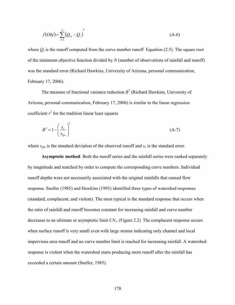
178

( ) ( )2

1

∑=

−=N

i

ioi QQObjf (A-6)

where Qi is the runoff computed from the curve number runoff Equation (2.5). The square root

of the minimum objective function divided by N (number of observations of rainfall and runoff)

was the standard error (Richard Hawkins, University of Arizona, personal communication,

February 17, 2006).

The measure of fractional variance reduction R2 (Richard Hawkins, University of

Arizona, personal communication, February 17, 2006) is similar to the linear regression

coefficient r2 for the tradition linear least squares

2

2 1

−=

Qo

e

s

sR (A-7)

where sQo is the standard deviation of the observed runoff and se is the standard error.

Asymptotic method: Both the runoff series and the rainfall series were ranked separately

by magnitude and matched by order to compute the corresponding curve numbers. Individual

runoff depths were not necessarily associated with the original rainfalls that caused flow

response. Sneller (1985) and Hawkins (1993) identified three types of watershed responses

(standard, complacent, and violent). The most typical is the standard response that occurs when

the ratio of rainfall and runoff becomes constant for increasing rainfall and curve number

decreases to an ultimate or asymptotic limit CN∞ (Figure 2.2). The complacent response occurs

when surface runoff is very small even with large storms indicating only channel and local

impervious area runoff and no curve number limit is reached for increasing rainfall. A watershed

response is violent when the watershed starts producing more runoff after the rainfall has

exceeded a certain amount (Sneller, 1985).

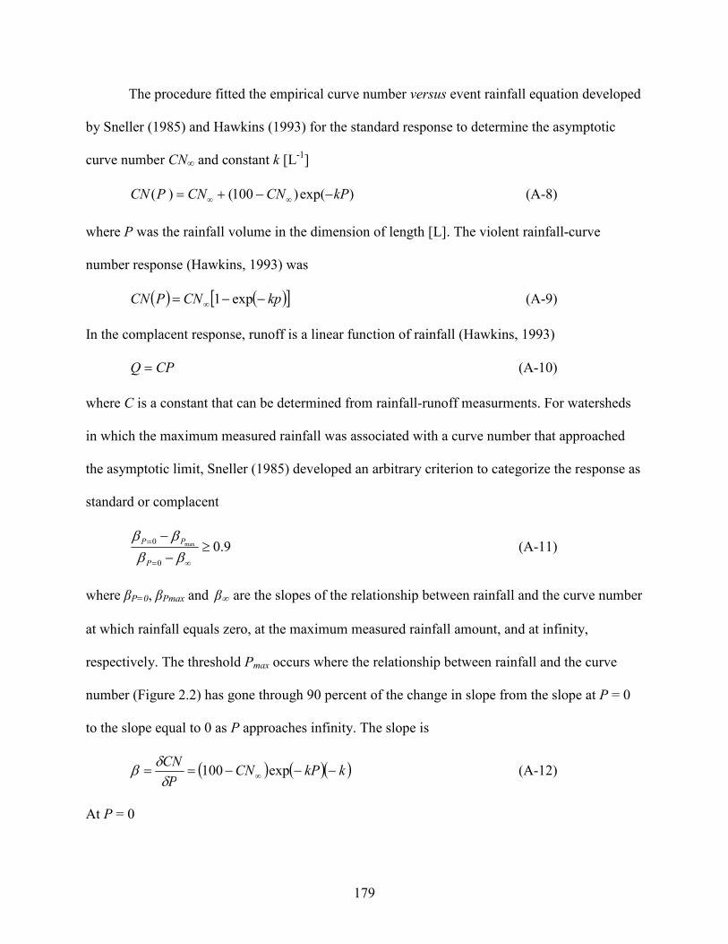
179

The procedure fitted the empirical curve number versus event rainfall equation developed

by Sneller (1985) and Hawkins (1993) for the standard response to determine the asymptotic

curve number CN∞ and constant k [L-1]

)exp()100()( kPCNCNPCN −−+= ∞∞ (A-8)

where P was the rainfall volume in the dimension of length [L]. The violent rainfall-curve

number response (Hawkins, 1993) was

( ) ( )[ ]kpCNPCN −−= ∞ exp1 (A-9)

In the complacent response, runoff is a linear function of rainfall (Hawkins, 1993)

CPQ = (A-10)

where C is a constant that can be determined from rainfall-runoff measurments. For watersheds

in which the maximum measured rainfall was associated with a curve number that approached

the asymptotic limit, Sneller (1985) developed an arbitrary criterion to categorize the response as

standard or complacent

9.00

0 max ≥−

−

∞=

=

ββ

ββ

P

PP (A-11)

where βP=0, βPmax and β∞ are the slopes of the relationship between rainfall and the curve number

at which rainfall equals zero, at the maximum measured rainfall amount, and at infinity,

respectively. The threshold Pmax occurs where the relationship between rainfall and the curve

number (Figure 2.2) has gone through 90 percent of the change in slope from the slope at P = 0

to the slope equal to 0 as P approaches infinity. The slope is

( ) ( )( )kkPCNP

CN−−−== ∞ exp100

δδ

β (A-12)

At P = 0

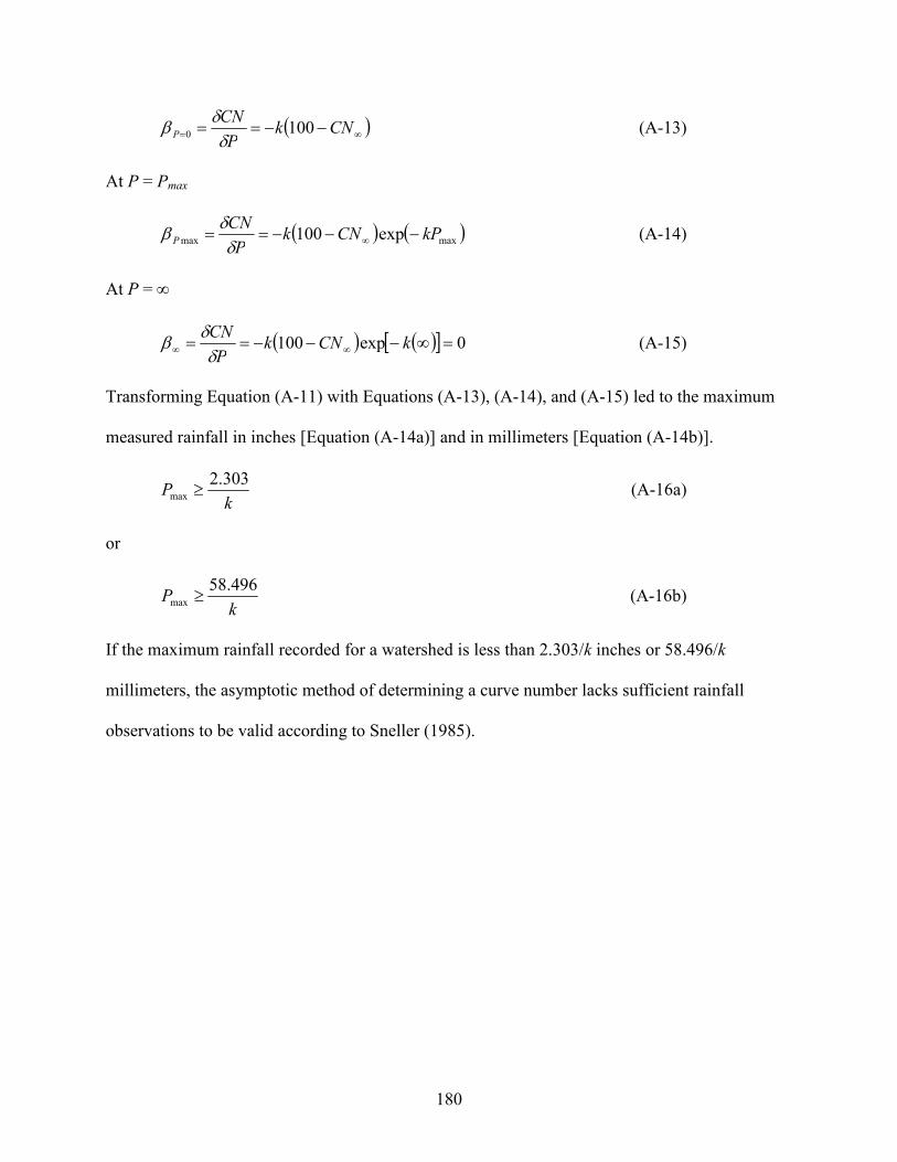
180

( )∞= −−== CNkP

CNP 1000 δ

δβ (A-13)

At P = Pmax

( ) ( )maxmax exp100 kPCNkP

CNP −−−== ∞δ

δβ (A-14)

At P = ∞

( ) ( )[ ] 0exp100 =∞−−−== ∞∞ kCNkP

CN

δδ

β (A-15)

Transforming Equation (A-11) with Equations (A-13), (A-14), and (A-15) led to the maximum

measured rainfall in inches [Equation (A-14a)] and in millimeters [Equation (A-14b)].

kP

303.2max ≥ (A-16a)

or

kP

496.58max ≥ (A-16b)

If the maximum rainfall recorded for a watershed is less than 2.303/k inches or 58.496/k

millimeters, the asymptotic method of determining a curve number lacks sufficient rainfall

observations to be valid according to Sneller (1985).

181

APPENDIX B

PROBABILITY DISTRIBUTIONS

• Probability density function (PDF) is any function f (x) that describes the probability

density in terms of the input variables in a manner described below.

f (x) is greater than or equal to zero for all values of x.

The total area under the graph is 1:

( ) 1=∫∞

∞−

dxxf (A1)

The actual probability can then be calculated by taking the integral of the function f (x) by

the integration interval of the input variable x. For example, the probability of the

variable X being within the interval [1, 5] would be

( ) ( )dxxfX ∫=≤≤5

1

51Pr (A2)

• Cumulative distribution function (CDF), also called probability distribution function

or just distribution function, describes the probability distribution for a real-valued

random variable X. For every real number x, the CDF of X is given by

( ) ( )xXPxFx x ≤=→ (A3)

where the right hand side represents the probability that the random variable X taken on a

value less than or equal to x. The probability that X lies in the interval (a, b] is, therefore,

F (b) – F (a) if a < b. A capital F for a cumulative distribution function is conventional in

contrast to the lower-case f used for probability density function. The CDF of f can be

defined in terms of the probability density function f as follows:

( ) ( ) 1== ∫∞

∞−

dttfxF (A4)

182

wher f (t) is a function which varies with time

• Empirical distribution function (EDF) is a cumulative probability distribution function

that concentrates probability (1/n) at each of the n numbers in a sample expressed as.

( ) ( )∑=

≤=n

i

in xXIn

xF1

1 (A5)

where I (Xi ≤ x) is an indicator of event (Xi ≤ x)

• Shape parameter (γ): is a parameter that allows a distribution to take on a variety of

shapes, depending on the value of the shape parameter.

• Location parameter (µ): is a parameter that simply shifts the graph left or right on the

horizontal axis

• Scale parameter (β): is a parameter that has an effect of stretching out or squeezing the

probability distribution function

• Normal distribution: is a distribution that has a general formula for the probability

density function which can be expressed as

( )( ) ( )

πβ

βµ

2

222−−

=xe

xf x ≥ µ; β > 0 (A6)

where µ is the location parameter and β is the scale parameter. The case where µ = 0 and

β = 1 is called the standard normal distribution. The equation for the standard normal

distribution is

( )π2

22xexf

−

= x ≥ 0 (A7)

Since the general form of probability functions can be expressed in terms of the standard

distribution, all subsequent formulas in this section are also given for the standard form

of the function in addition to the general form.

183

• Lognormal distribution: A variable X is lognormally distributed if Y = Ln (X) is

normally distributed with "Ln" denoting the natural logarithm. The general formula for

the probability density function of the lognormal distribution is

( )( )( )( ) ( )( )

( ) πγµ

γβµ

2

222//ln

−=

−−

x

exf

x

x ≥ µ; β, γ > 0 (A8)

where γ is the shape parameter, µ is the location parameter and β is the scale parameter.

The case where µ = 0 and β = 1 is called the standard lognormal distribution. The

equation for the standard lognormal distribution is

( )( ) ( )( )

πγ

γ

2

222/ln

x

exf

x−

= x ≥ 0; γ > 0 (A9)

• Gamma distribution: is a distribution that has a general formula for the probability

density function

( ) ( ) ( )

( )γββµ βµγ

Γ−

=−−− xex

xf

1

x ≥ µ; γ, β > 0 (A10)

where γ is the Shape parameter, µ is the location parameter β is the scale parameter, and Г

(a) is the gamma function which has the formula

( ) dteta ta −∞

−∫=Γ0

1 (A11)

The case where µ = 0 and β = 1 is called the standard Gamma distribution and described

as

( ) ( ) ( )

( )γ

γ

Γ=

−− xexxf

1

x ≥ 0; γ > 0 (A12)

• Weibull distribution: has a general form of probability density function

184

( )( )

( )( )( )γβµγ

βµ

βγ /

1

−−

−

−= xe

xxf x ≥ µ; γ, β > 0 (A13)

where γ is the shape parameter, µ is the location parameter and β is the scale parameter.

The case where µ = 0 and β = 1 is called the standard Weibull distribution. The case

where µ = 0 is called the 2-parameter or standard Weibull distribution. The equation for

the standard Weibull distribution reduces to

( ) γγγ xexxf −−= )1( x ≥ 0; γ > 0 (A14)

since the general form of probability functions can be expressed in terms of the standard

distribution.

• Goodness-of-fit tests: indicate whether a sample comes from a specific distribution.

Statistical techniques often rely on observations having come from a population that has a

distribution of a specific form (e.g., normal, lognormal, and Weibull).