Embed Size (px)
Citation preview
Rainfall Intensity in DesignRainfall Intensity in Design
Ted Cleveland University of Houston
David Thompson RO Anderson, Inc.
TRB January 2008
Ted Cleveland University of Houston
David Thompson RO Anderson, Inc.
TRB January 2008
AcknowledgementsAcknowledgements
Texas Department of Transportation– Various projects since FY 2000.– Current: 0-6070 Use of Rational and Modified
Rational Method for Drainage Design.
William H. Asquith, USGS– Research colleague who provided much of the
ideas and authored the R package that makes the simulations possible.
Texas Department of Transportation– Various projects since FY 2000.– Current: 0-6070 Use of Rational and Modified
Rational Method for Drainage Design.
William H. Asquith, USGS– Research colleague who provided much of the
ideas and authored the R package that makes the simulations possible.
IntroductionIntroduction
Result of a question:– “After all, how hard can it rain?”
Intensity has variety of uses– BMP design – Rational method
Examine use of recent tools:– Are estimated intensities consistent with
observations?
Result of a question:– “After all, how hard can it rain?”
Intensity has variety of uses– BMP design – Rational method
Examine use of recent tools:– Are estimated intensities consistent with
observations?
Data SourcesData Sources
Texas specific:– Asquith and others (2004)– Williams-Sether and others (2004)– Asquith and others (2006)
Global Maxima– Jennings (1950), Paulhus (1965), Barcelo and
others (1997), Smith and others (2001)
Texas specific:– Asquith and others (2004)– Williams-Sether and others (2004)– Asquith and others (2006)
Global Maxima– Jennings (1950), Paulhus (1965), Barcelo and
others (1997), Smith and others (2001)
Data SourcesData Sources
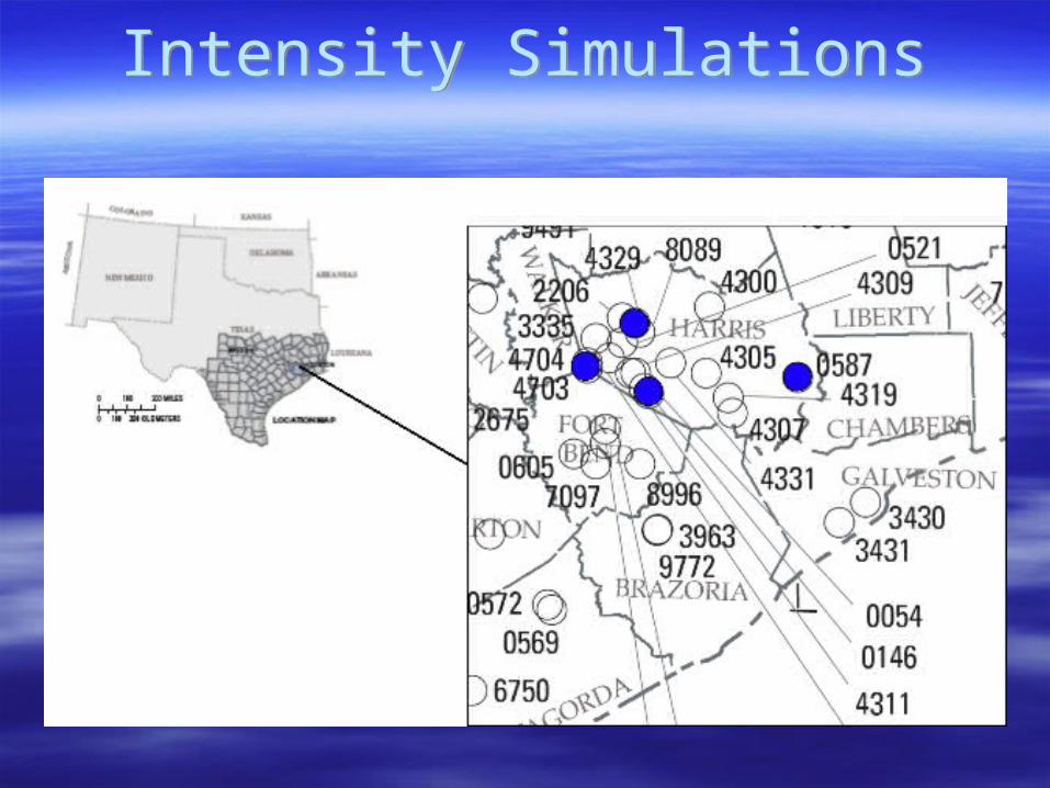
Asquith and others (2004).– 92 stations (up to 135).– 1600 paired events.
Asquith and others (2004).– 92 stations (up to 135).– 1600 paired events.
QuickTime™ and aTIFF (Uncompressed) decompressor
are needed to see this picture.
Empirical HyetographsEmpirical Hyetographs
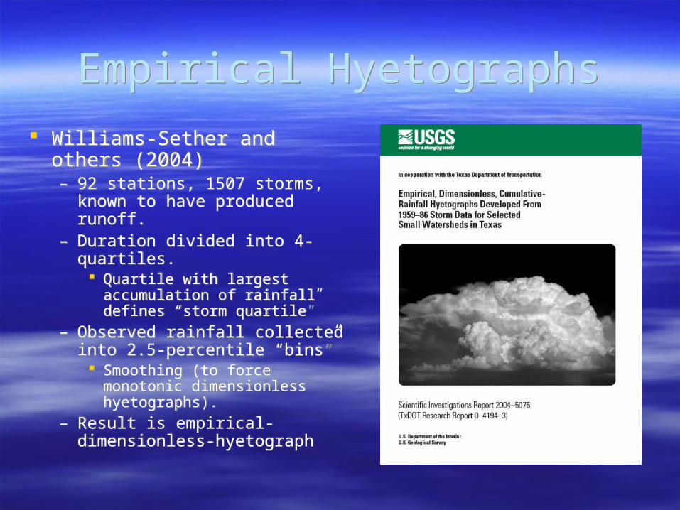
Williams-Sether and others (2004)– 92 stations, 1507 storms, known
to have produced runoff.– Duration divided into 4-quartiles.
Quartile with largest
accumulation of rainfall defines “storm quartile”
– Observed rainfall collected into 2.5-percentile “bins”
Smoothing (to force monotonic dimensionless hyetographs).
– Result is empirical-dimensionless-hyetograph
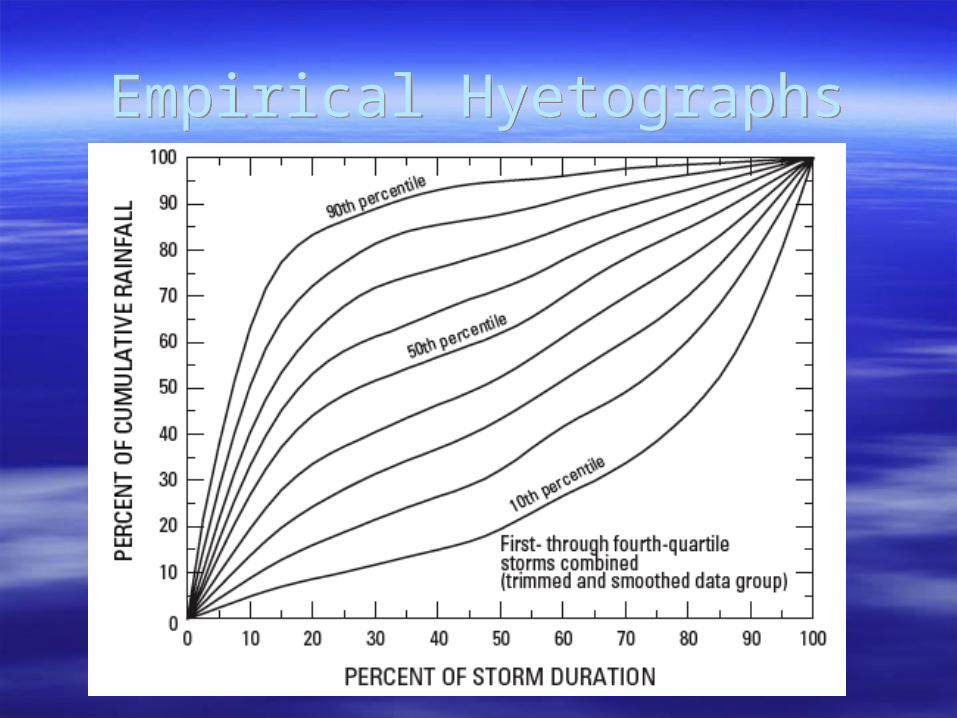
Empirical HyetographsEmpirical Hyetographs
Empirical HyetographsEmpirical Hyetographs
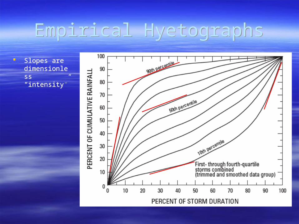
Slopes are dimensionless “intensity”
Slopes are dimensionless “intensity”
Intensity SimulationsIntensity Simulations
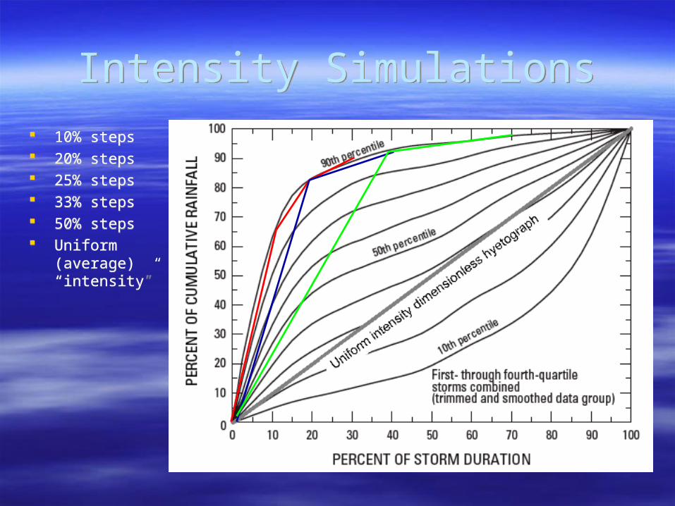
10% steps 20% steps 25% steps 33% steps 50% steps Uniform
(average) “intensity”
10% steps 20% steps 25% steps 33% steps 50% steps Uniform
(average) “intensity”
Intensity SimulationsIntensity Simulations
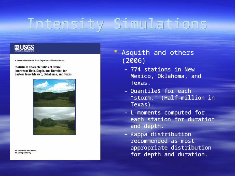
Asquith and others (2006)– 774 stations in New Mexico,
Oklahoma, and Texas.– Quantiles for each “storm.”
(Half-million in Texas).– L-moments computed for
each station for duration and depth.
– Kappa distribution recommended as most appropriate distribution for depth and duration.
Asquith and others (2006)– 774 stations in New Mexico,
Oklahoma, and Texas.– Quantiles for each “storm.”
(Half-million in Texas).– L-moments computed for
each station for duration and depth.
– Kappa distribution recommended as most appropriate distribution for depth and duration.
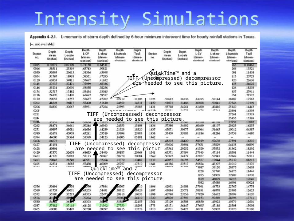
Intensity SimulationsIntensity Simulations
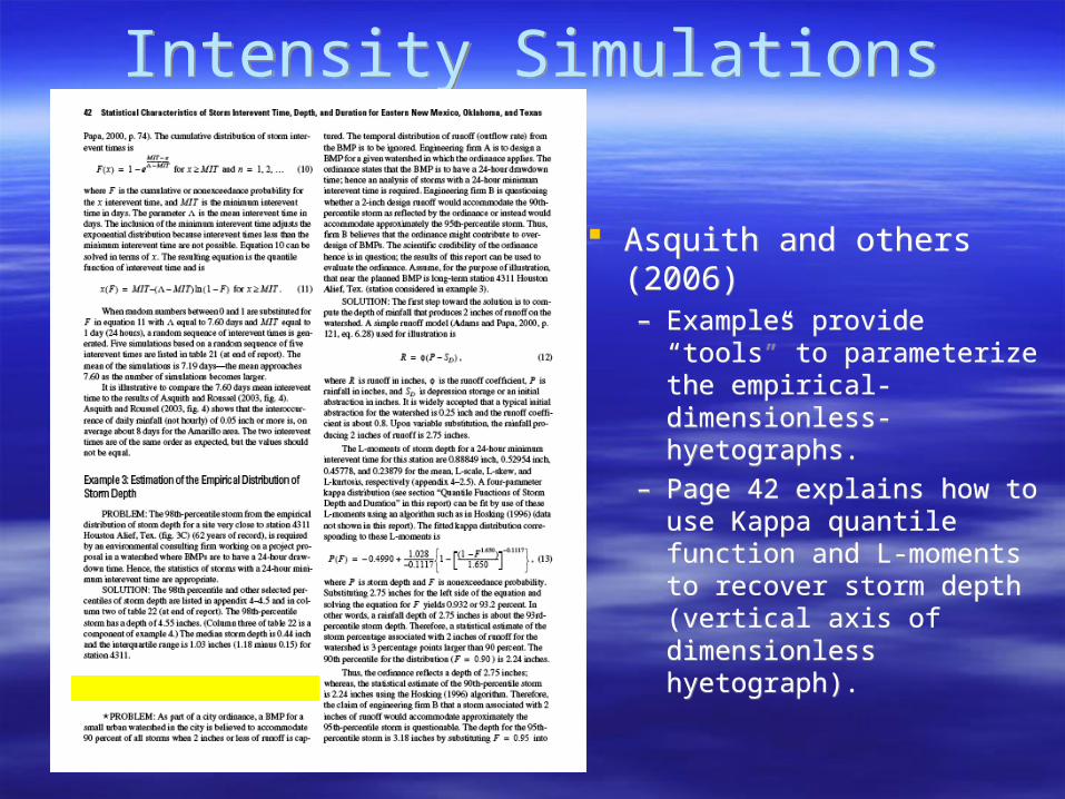
Asquith and others (2006)– Examples provide “tools” to
parameterize the empirical-dimensionless-hyetographs.
– Page 42 explains how to use Kappa quantile function and L-moments to recover storm depth (vertical axis of dimensionless hyetograph).
Asquith and others (2006)– Examples provide “tools” to
parameterize the empirical-dimensionless-hyetographs.
– Page 42 explains how to use Kappa quantile function and L-moments to recover storm depth (vertical axis of dimensionless hyetograph).
Intensity SimulationsIntensity Simulations
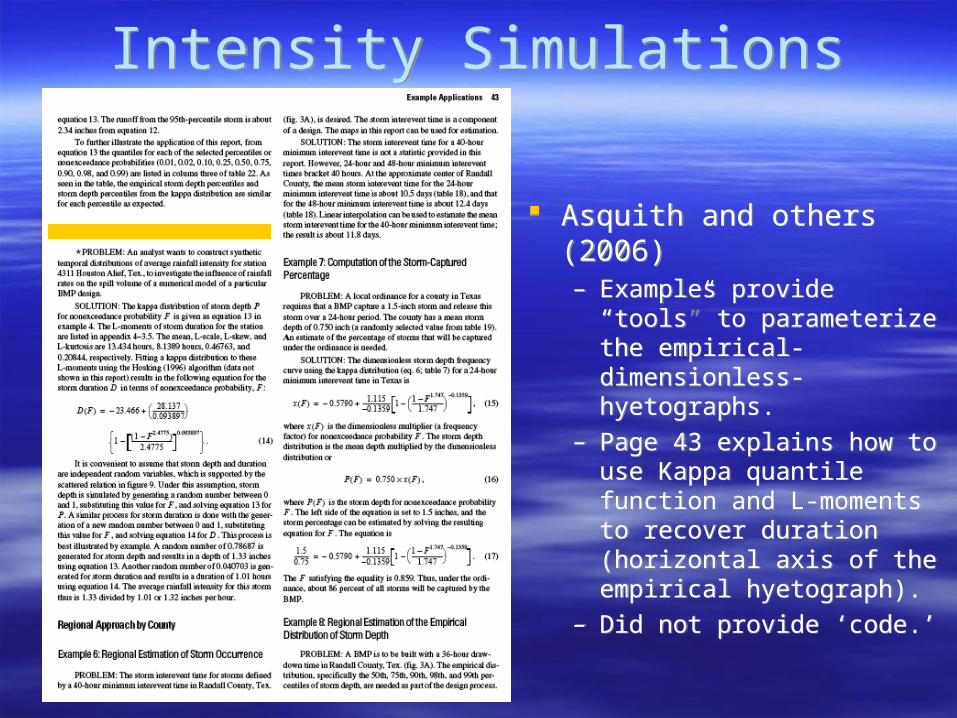
Asquith and others (2006)– Examples provide “tools” to
parameterize the empirical-dimensionless-hyetographs.
– Page 43 explains how to use Kappa quantile function and L-moments to recover duration (horizontal axis of the empirical hyetograph).
– Did not provide ‘code.’
Asquith and others (2006)– Examples provide “tools” to
parameterize the empirical-dimensionless-hyetographs.
– Page 43 explains how to use Kappa quantile function and L-moments to recover duration (horizontal axis of the empirical hyetograph).
– Did not provide ‘code.’
Intensity SimulationsIntensity Simulations
Intensity SimulationsIntensity Simulations
QuickTime™ and aTIFF (Uncompressed) decompressor
are needed to see this picture.
QuickTime™ and aTIFF (Uncompressed) decompressor
are needed to see this picture.
QuickTime™ and aTIFF (Uncompressed) decompressor
are needed to see this picture.
QuickTime™ and aTIFF (Uncompressed) decompressor
are needed to see this picture.
Intensity SimulationsIntensity Simulations
Asquith (2007) – LMOMCO package in R– Provides the necessary ‘code’ to make such computations.
Asquith (2007) – LMOMCO package in R– Provides the necessary ‘code’ to make such computations.
QuickTime™ and aTIFF (Uncompressed) decompressor
are needed to see this picture.
Intensity SimulationsIntensity Simulations
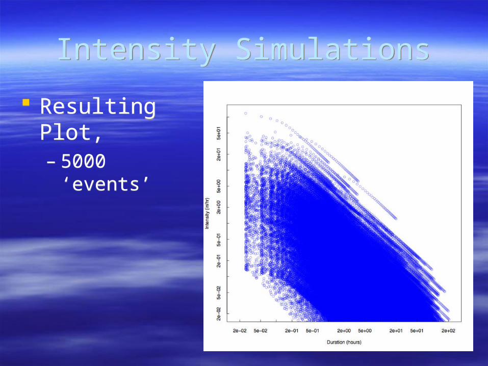
Resulting Plot,– 5000 ‘events’
Resulting Plot,– 5000 ‘events’
Comparisons to Prior WorkComparisons to Prior Work
Asquith and Roussel (2004)– L-moments
analysis.– Product similar to
TP-40; HY-35
Asquith and Roussel (2004)– L-moments
analysis.– Product similar to
TP-40; HY-35
QuickTime™ and aTIFF (Uncompressed) decompressor
are needed to see this picture.
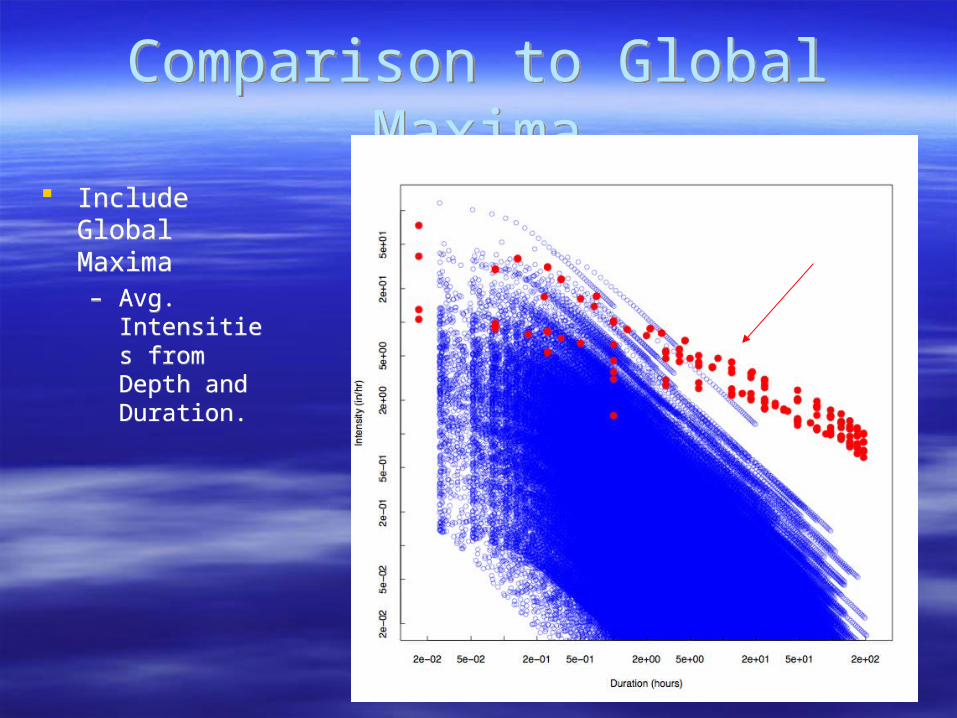
Comparison to Global MaximaComparison to Global Maxima
Include Global Maxima– Avg.
Intensities from Depth and Duration.
Include Global Maxima– Avg.
Intensities from Depth and Duration.
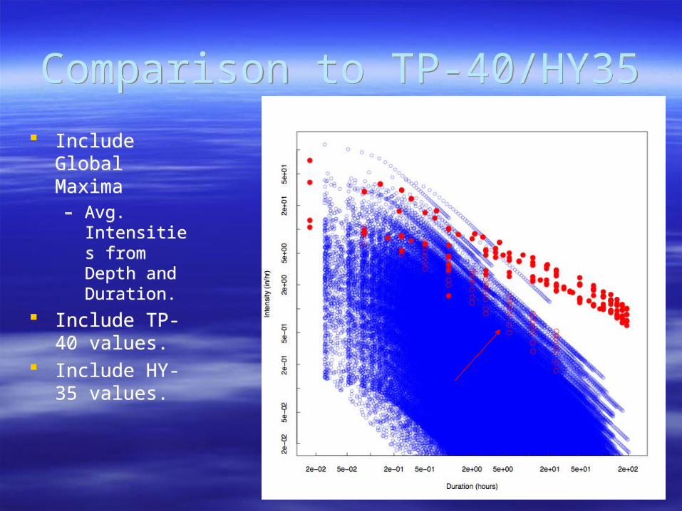
Comparison to TP-40/HY35Comparison to TP-40/HY35
Include Global Maxima– Avg.
Intensities from Depth and Duration.
Include TP-40 values.
Include HY-35 values.
Include Global Maxima– Avg.
Intensities from Depth and Duration.
Include TP-40 values.
Include HY-35 values.
Empirical PercentilesEmpirical Percentiles
Empirical ‘Percentiles’– Count fraction
above and below line.
– Fraction establishes percentile.
– Line is an ad-hoc model.
– “Design” Equation is from TxDOT manual
Empirical ‘Percentiles’– Count fraction
above and below line.
– Fraction establishes percentile.
– Line is an ad-hoc model.
– “Design” Equation is from TxDOT manual
QuickTime™ and aTIFF (Uncompressed) decompressor
are needed to see this picture.
Empirical PercentilesEmpirical Percentiles
COH IDF Overlay.– 2-year line is
about the 95% empirical percentile.
COH IDF Overlay.– 2-year line is
about the 95% empirical percentile.
QuickTime™ and aTIFF (Uncompressed) decompressor
are needed to see this picture.
ConclusionsConclusions
Results are consistent with prior work. Results are within the global envelope. Differences at higher duration - Texas
storms less intense if long. Rare (99th-percentile) estimates about the
same. Median (50th-percentile) quite different.
– Consequence of what simulations actually represent.
Results are consistent with prior work. Results are within the global envelope. Differences at higher duration - Texas
storms less intense if long. Rare (99th-percentile) estimates about the
same. Median (50th-percentile) quite different.
– Consequence of what simulations actually represent.
Future DirectionsFuture Directions
Biggest assumption is independent depth and duration.– There is evidence that these variables are
highly coupled, especially for longer durations.
Conditional dependence should be examined.– Important for water quality issues.
Biggest assumption is independent depth and duration.– There is evidence that these variables are
highly coupled, especially for longer durations.
Conditional dependence should be examined.– Important for water quality issues.