10272-101

REPORT DOCUMENTATAlION 1" REPORT NO. I 2. I. "93-'7"18 PAGE N8FIISI-HOe7

•. TIll 1IId ...... 5. AIport Oat. September 1 Ng

Nonlnear Selamlc AnaIytIs 01 Rmbced Concr .. BuIlding., PI'Iae I Technical Report

•• 7.~hor(.) MoM. Ettouney. R.P. DMdazIo •• PwdDnNnI 0IganIaII0n ""*' No.

I.,...... ~I MImI Md MnIa 10. ~1IIkIWoItI Unit No.

Wlldlng.r AMociId. 11. CorhcI(C) 01' Clrln(CI) No. 333 Seventh Avenue

Nft Yot1<, NY 10001 tel (G) 1818880254

12. _.rio .. ~ian ....... lIId ....... 13. Tp CII AIpaft • Pwriad c-.d

DI..ctorat. for EnglnHrlng. 8m" a'-n ... Innovation ReIearch (SaIR) SBIRPh ... 1

~Ion" Sc:ience Four*Ian. Wuhing'.on DC 20550 1 ••

~

15. 1uAI111MIUIy NaeIe

. 16. Aba1racr (limit: 200 words)

-S ThrM new concepII •• deecrhd: (1) an efficient ,.inforwd concnte mateMI rnoHI buec:I on pIMtlcity ttwory; (2) an anaIytk:al 8OIutlon to, the integration along the length of the nonU,.., beam d.tannatlona; and (3) a dletrbutlon 01 deformation technlqu. which aIIoM the pr ... rv.1on of local nodal bulding rotations while performing the .xpllcll dynamic anaJytls at a tim •• t.., correepondlng to the globtl floor rot.ions. Thea. dtYelopmtnts wer. impl.m.nted Into a prafOtypt PC-butd coll1P'Dr program. B.nchmark analy ... we,. performed to indlcat. the eccur.cy and .fflcitncy 01 the mathod. E:: -

17.~AnIIVIII"~

Dynamic atructu,. aMIyaIa R.Inforctd concrete 0eI0rmati0n Platlc properties

Build.

b.~T_

Sellmlc anIIIyIia Nonlinear dynamic analylil

G:eo.I~

, .. AwMay ......... NTIS ,I. ......, CIIM (TIIII AIpad) 1'.Mo. ........

10 • ......, CIIII (TIIII ,.. 12. .....

,-_ . ., - ,--- ......, ........ ru.- .,. , ... ,,,

NONLINEAR SEISMIC ANALYSIS OF REINFORCED CONCRETE BUILDINGS

Mohammed M. Ettouney and Raymond P. Daddazio Weidlinger Auociates, Inc. 333 Seventh A venue New York, NY 10001

30 September 1989

Phase I Technical Report

NSF/ISI-89061

PB93-1711118

THIS MATERIAL IS BASED UPON WORK SUPPORJ'ED BY THE NATIONAL SCIENCE FOUNDATION UNDER. AWARD NUM­

BER. ISI·Me02I4. ANY OPINIONS.FlNDINGS. AND CONCLUSIONS OR. RBCO .... BNDATIONS EXPRESSED IN THIS PUB­

LICATION ARE 11IOSE OF THE AU11IOR(S) AND DO NOT NECESSARILY IlEFLBCf THE VIEWS OF THE NATIONAL

SCIENCE FOUNDATION.

REPRODUCED BY

U.S. DEPARTMENT OF COMMERCE NATIONAL TECHNICAL NFORMATION SERVICE SPRINGFIElD. VA. 22161

1 • INTRODUCTION

Damage to reinforced concrete (RC) buildings resulting from an earthquake is a serious event. The economic los8 is always evident and in certain catastrophic cases even I08S of life may result. Many analysis techniques, that aid in the understanding and mitigation of this problem have been developed. Methods for material nonlinear seismic a.nalysis of RC buildings can be divided into two general categories. In the first category are methods specialized to high rise structures [Anag-1I0stopouios 1972; Wilson 1975], that make certain assumptions which can improve the efficiency of the calculations. In the second category are methods that use general purpose finite element programs to solve the problem. The practicing engineer usually finds it difficult to use methods in ei ther of these two categories because of the following reasons.

The specialized methods in the first category are usually developed for research purp08es. This makes them virtually inaccessible to design engineers. In addition, some of these approaches a.re based on certain assumptions which can reduce the range of applicability of such methods.

Methods in the second category which use general purp08e finite element programs are usually too costly and inefficient to be used during the design process of a typical RC structure. In a.ddition. the proper force-deformation relations for RC elements (beams. columns, shear walls or slabs) are usually not available in these programs.

The above facts show the need for a simple and accurate nonlinear seismic analysis method for RC structures which can be made readily available to practicing engineers. Although the need for such a method has existed for a some time, it was not generally perceived since in practice, a linear analysis approach combined with the popular response spectrum technique [ATC 1978; UBC 1985] has been used to analyze and design RC structures. However, several recent developments suggest that a change in this type of approach may be necessary. These developments may make it essential for cesign engineers to investigate the nonlinear behavior of the building under consideration. The following is a brief discussion of these developments.

A recent study by Seeber, 1988 suggests that the potential exists for major seismic events to occur on the east coast of the United States. It was also reported [Atkinson 1988: Somerville 1988 1 that because of different geologic conditions, these seismic events may be different in terms of frequency content, duration and acceleration amplit1lde from th08e events typical of the west coast. Hence,current design methods which are based on west cout seismic events may not be directly applicable to buildings on the east coast. These condit.ions make it very important that engineers involved in the analysis and design of buildings in the eastern US have available a sjmple, and accurate method for the material nonlinear analysis of RC buildings (especially existing ones) subjected to east coast specific seismic events.

The importance of the above mentioned facts is amplified because most residential RC build­ings in the eastern US use flat plate (slab) type construction for the flooring system [Moehle, J.P., 1988 and Weidlinger, P. and Ettouney, M.M., 19881. Using conventional nonlinear anal­ysis methods available in general purpose finite element programs for the analysis of these types of buildings is not a. practicable alternative for the practicing engineer, technically nor economically. The need for a simple method to analyze this type of construction is apparent.

Current research [Hall 1988] has focused on the applicability of the response spectra approach in the design of structures which must resist seismic shaking. Although a response spectra is a simple and elegant input to seismic design and analysis problems, it must also be recognized that the method cannot adequately represent the duration of a seismic event nor the hysteresis

2

cycles in a structure subjected to an earthquake. It is important to account for both facts jf a realistic assessment of the behavior and damage of the building during a seismic event is to be achieved. In order to evaluate equivalent hystere~is cycles for a system beyond its elastic range, a nonlinear time history analysis is needed. Sinc.~ most buildings are at present designed to dissipate energy during seismic events through lar,.e inelastic deformations the need for an efficient and accurate method for the nonlinear analysis of RC structures is clear.

Finally, advances in the capacity of personal computers coupled with their proliferation makes it practical from both a technical and economic viewpoint to develop an efficient computer program for the problem in question which can be executed on these machines. Such a pro­gram will bring the capability of nonlinear seismic analysis of RC buildings to the desktop of practicing engineers.

Current Work The problem to be addressed in Phase I is the development of a method for the damage assessment of RC buildings subjected to earthquakes. The resulting technique has to be accurate for such structures and easily usable by engineers.

The specific objectives are:

1. to develop the formulation for two dimensional nonlinear seh;mic analysis of reinforced concrete buildings,

2. to incorporate the formulation of step 1 in a. special purpose, prototype computer code, and

3. to perform some case study runs to investigate the formulation as well as the program.

Section 2 of this report describes an innovative methodology which accounts for the nonlin­ear behavior of RC high rise buildings during an earthquake in an accurate and efficient way. Specifically, we will introduce three new concepts, they are:

i- a new efficient nonlinear reinforced concrete material model. which couples axial and bending deformations utilizing an accurate plasticity theory approach,

ii- an analytical solution for the "integration along the length" of the nonlinear beam defor­mations, and

iii- a "distribution of deformation" technique, which allow the preservation of local nodal building rotations, yet uses a long integration time step which corresponds to the global floor rotations.

Section 3 describes the c.omputer code SNORT which was developed for the purpose of this research and which implements the above mentioned methodology. Finally, the program will be used to evaluate simple structures subjected to base motions in section 4. The relevant conclusions and suggestions for Phase II future work will be made in section 5.

3

2 . THEORETICAL BACKGROUND

"2 . 1 The BOW Plasticity Model/Integra.tion through the thickness

Nonlinear force deformation relations for reinforced concrete members have been developed by numerous authors, e.g. [Chung et al, 1987]. Several models have been recommended and used for this purpose. These material models can be divided into two main categories:

i· Continuum models: These models use plasticity theories to simulate the stress-strain be­havior in plain concrete ILevine, H.S., 1982, Baylor, J. and Wright, J., 1987, and Mould, J.C. and Levine. H.S., 1987]. The concrete body is modeled using two, or three dimensional, finite elements. Reinforcing steel is usually modeled by linear or nonlinear elements. This approach. although fairly accurate for several classes of problems, is certainly not economical for cases involving seismic loadings due to the tremendous amount of calculations needed to simulate the different members of the structures using two or three dimensional continuum elements, a.nd integrating these motions through the whole time span of the earthquake. Also, the mod­eli&g of crack opening and dosing, interaction between reinforcing steel and plain concrete, degradation of strength and stiffness of the composite reinforced concrete beam as compared to the plain concrete body, are all modeling problems which have not been sufficiently studied by the research community to date.

ii· Beam models: These models relate the nonlinear behavior of resultant forces in the cross section of beama to the pertinent beam deformations IAganostopolous, S.A., 1972 and Chung, Y.S., et al. 1987]. This approach is economical since it avoids the costly integration through the thickness which is needed for the continuum model~. The advantages of this modeling technique are that it accounts for tht: interaction between reinforcing steel and the surrounding concrete in a natural way, treatment of crack openings and closings is embodied in the model, and, the simulation of the «!egradation of both strength and stiffness of the whole composite section is straightforward. However, only scalar moment·curvature relations have been used to simula ~e the nonlinear reinforced concrete behavior. To the best of our knowledge, the coupling betwt!en axial and shearing forces with the bending moments has not been accounted for in any of these models. This can present a serious accuracy problem especially for reinforced concrete columns in the lower stories of buildings, where the axial Corces are relatively large. Also it may result in inaccurate solutions for buildings where the p.~ effects are large.

In this study we will introduce a nonlint>aT reinforced concrete beam material model which will account for the coupling between all resultant forces of a 2D beam. It is based on plasticity theory principles with an associated flow rule, which permits us to account for the coupling of forces and deformations. We will refer to this model as the "BOW" model, since the yield surface moves &f a. bow. as we wiD see later.

2 - 1 . 1 Plasticity Equations of the BOW Model

2 . 1 . 1 . 1 Incremental Relations

Consider the cross section of the 2D beam in figure 1, which shows the internal forces (N,M) and the equivalent deformations (£,4» of the cross section, where N, M. l and 4> are the axial force, the bending moment, axial deformation and curvature, respectively. We will also use the following definitions:

4

For incremental loading, we have:

ST = [N,M)

= Total force vector

e T = [£,4» = Total deformation vector

de = de~ + de'

de~ = Incremental elastic deformation vector

de" = Incremental plastic deformation vector

(1)

with de representing the total incremental deformation vector. The weU known elastic law [Martin, J .B .• 19751 can be stated as:

dS= D(de-de'} (2)

D = Current elastic matrix

= K~ [: ~] where A and I represent the equivalent area and moment of inertia of the cross section under consideration, respectively. Note that Ke is the current elastic modulus. It is allowed to vary in order to simulate the degradation of stiffness in the BOW model.

2 . 1 - 1 - 2 Yield Surface

The yield surface( s), F = 0, figure 2, will be represented by a family of curves ill the form of:

F = F(M,N,a-) = 1 + ala-M + ala-M'l + a3N + a4N'l + asa-M N (3)

where a- is a hardening parameter which completely defines the location of the current yield surface. The parameters al, ... as are constants which define the shape of the yield surface family, their values depend on the beam cross sectional geometry and reinforcement. Note that the choice of this specific shape of yield surface achieves the foUowing goals:

I - It allows hardening only for bending moment, no axial force hardening. ii - Accurate simulation of different force combinations which are shown in figure 2 (points 'a'

through 'e' on the yield curve) ; these points represent the following force combinations regions:

a- Axial tension. b- Pure bending. c- Axial compression, below balance point. d- Balance point. e- Axial compression, above balance point.

5

For the purpose of this study, the factors 41, ••• 45 were calculated using the interaction diagram [Winter, G. and NilllOn, A. H., 1972] for the cross section under -:onsideration. For non­symmetric beam reinforcement, two families of yield surfaces F+. F" will be used, figure 2. The derivatives of F can be expressed as:

F,j = [F,N F,M] = [(43 + 2a. .. N + 4,0- M) (410- + 2C120-2 M + 4,0-N)]

F,o- = (aiM + 262Q* M2 + 4,M N)

2 . 1 . 1 . 3 Flow Rule

We will enforce now the well known flow rule:

for F=O and

and

for or F=O and

(4)

(5)

(6)

(7)

where ..\ is a scalar value[Martin, J.B., 1975]. It can be shown that, using the condition F = 0, ..\ can be expres'led as:

..\ [ F,iD 1 d = F,iDF.s-F,o-AF,M e (8)

where A = A (0*) will be discussed later. It will be used in a fashion similar to [Bieniek,M.P. and Funaro, J. R. 1976], except that they were considering meta.llic type materials.

2 • 1 • 1 - 4 Tangent Stiffness

The nonlinear tan,gent stiffness of the crosa section can be written as:

dS = D (de - ..\F,s )

= Dtde

and the expression for the tangent stiffness, D t , is:

Dt - D [1- [ F .iD 11 - F,iDF,s -FlO- AF,M

2 - 1 . 2 Hardening Parameter

(9)

(10)

Numerous results are available [Clough. R.W., and Johnson, S.B., 1966, and Wakabayuhi, M., 1986] from testa of the behavior of reinforced concrete beams. Moet of thoee tests are for uniaxial bending (N = 0) loading. Hence we can design our pluticity "BOW" model to be consistent with

6

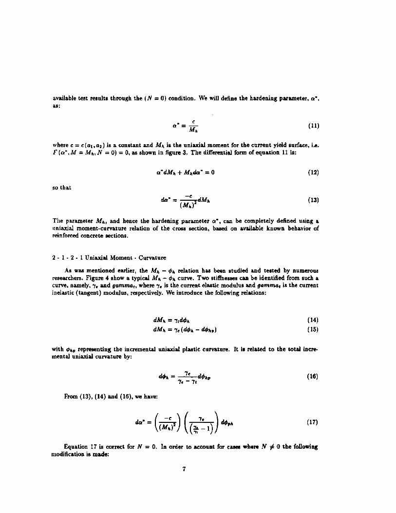
available test results through the (N = 0) condition. We will define the hardening parameter, 0", as:

" C Q =-

Mia (11)

where c = c (aI, a2) is a constant and M" is the uniaxial moment for the current yield surface, i.e. F (0" ,M = Mia, N = 0) = 0, as shown in figure 3. The differential form of equation 11 is:

(12)

so that

(13)

The parameter M", and hence the hardening parameter 0", can be completely defined using a uniaxial moment-curvature relation of the cross section, based on available known behavior of reinforced concrete sections.

2 - 1 - 2 - 1 Uniaxial Moment - Curvature

As was mentioned earlier, the M" - ,pia relation has been studied and tested by numerous researchers. Figure 4 show a typical M" - t/JIa curve. Two stiffnesses can be identified from such a curve. namely, "'fe and gammA" where "'fe is the current elastic modulus and gAmmA, is the current inelastic (tangent) modulus, respectively. We introduce the following relations:

dM" = 'Ttdt/J" dM" = 'Te (dtPIa - diP",)

(14)

(15)

with ,pia, representing the incremental uniaxial plastic curvature. It i. related to the total incre­mental uniaxial curvature by:

(16)

From (13), (14) and (16), we have:

(17)

Equation 17 is correct for N = O. In order to account for cases where N ;. 0 the followiq modification i. made:

7

CJ'088 section is in compresaion

Croes section is in tension

(18)

(19)

(20)

(21)

(22)

Note that {3 is a calibration factor which is unity in the present study. Figure 3 shows Nc aad NT. which are the ultimate axial compressive and tensile forces for the crOll section, respectively. Finally. equation 18 can be summarized as:

(23)

where A is the factor which was introduced in equation 8.

2 • 1 . 2· 2 Composition of M,. - q,,. Rel&tion

The plasticity equatioaa of the "BOW" model make it simple to introduce different features of the nonlinear behavior of reinforced concrete beams into the model without undue difficulty. Figure 5 show a typical M" - q,,, curve with the different f'eatures which have been incorporated in the "BOW" in the present study. It illustrates the first hysteresis loop. A brief discussion of each of these features will follow:

i· Degradation of Stiffness The elastic moduli 7ea. 7d and 7e3 are such that 711 ~ 7c2 ~ 7.3 which insure the simulation of the required loss of stiffness. The current elastic modulus 7. is evaluated as:

where 7e1 iI the virgin elastic modulus, 1.+ and 1.- are the smallest secant moduli in the latest positive and negative loading conditioaa, respectively. The conditions:

el +!2 +e3 = 1 el::S; 1

e2::S; 1

e:s ::s; 1

(25)

(26)

(27)

(28)

will insure the required degradation of stiffness. The parameters el,2,3 can be evaluated by ue of test results.

ii - Degradation of Strength A method similar to [Chung, Y.S., et ai, 1987J will be folloncl in this work to insure degradation of strength of' the cross section. The main &Alvant .. of tlUl method it that the resulting 1011 of' Itreqth il dependent on the total foree • deformation

8

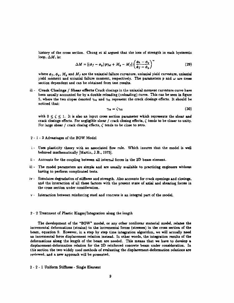
history of the cross section. Chung et al argued that the loss of strength in each hysteretic loop, ~M, is:

~M = [(<1>,- </),,)1'1., + M" - MIl (!; = ::) eM (29)

where tPI' tPlI' My and MI are the uniaxial failure curvature, uniaxial yield curvature, uniaxial yield moment and uniaxial failure moment, respectively. The parameters p and w are croes section dependent and can be obtained from test results.

iii - Crack Closings / Shear eff'eet. Crack closings in the uniaxial moment curvature curve have been usually accounted for by a double reloading (unloading) curve. This can be seen in figure 5, where the two slopes denoted 'Yt4 and 'YtS repretlent the cra.ck closings effects. It should be noticed that:

'Yt4 = ('Yt5 (30)

with 0 ~ ( ~ 1. It is also an input cross section parameter which represents the shear and crack closings effects. For negligible shear I crack dosing effects, ( tends to be closer to unity. For large shear I crack closing effects, ( tends to be close to zero.

2 - 1 . 3 Advantages of the BOW Model

i-Uses plasticity theory with an associated flow rule. Which insures that the model is well behaved mathematically [Martin, J.B., 1975).

ii - Accounts for the coupling between all intern'" forces in the 2D beam element.

iii - The model parameters are simple and are usually available to practicing engineers without having to perform complicated tests.

iv - Simula.tes degradation of stiffness and strength. Also accounts for crack openings and closings, and the interaction of all these factors with the present state of axial and shearing forces in the cross section under consideration.

v - Interaction between reinforcing steel and concrete is an integral part of the model.

2· 2 Treatment of Plastic Hinges/Integration along the length

The development of the "BOW" model, or any other nonlinear material model, relates the incremental deformations (strains) to the incremental forces (stresses) in the cross section of the beam, equation 9. However, in a step by step time integration algorithm, we will actually need an incremental force displacement relation instead. In other words, the integrat.ion results of t.he deformations along the length of the beam are needed. This means that we have to develop a displacement-deformation relation for the 2D reinforced concrete beam under consideration. In this section the two widely used methods of evaluating the displacement-deformation relations are reviewed, and a new approach will be presented.

2 - 2 - 1 Uniform Stiffness· Single Element

9

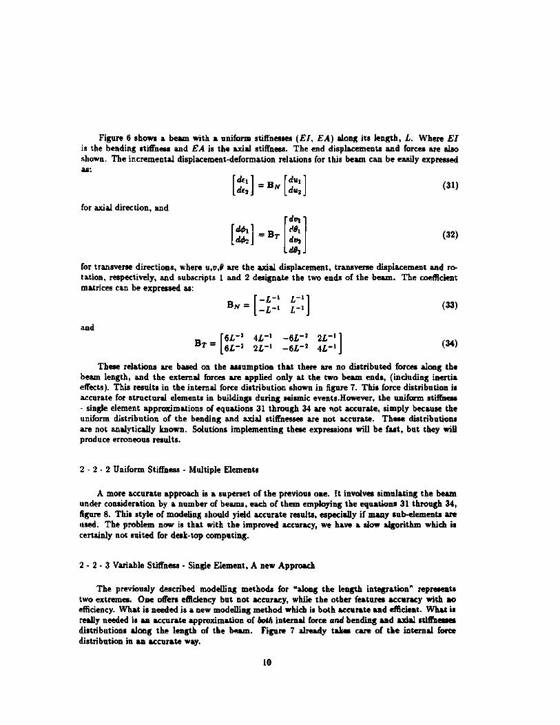
Figure 6 shoWl a beam with a uniform stiffneues (EI, EA) along its length, L. Where EI is the bending stiffness and EA is the axial stiffness. The end displa.cements and forces are also shown. The incremental displacement-deformation relations for this beam can be easily expressed as:

(31)

for axial direction, and

(32)

for transverse directions, where u,v,9 are the axial displacement, transverse displacement and r0-

tation, respectively, and subscripts 1 and 2 designate the two ends of the beam. The coefficient matrices can be expressed as:

and

L-l] L-l (33)

(34)

These relations are based. on the assumption that there are no distributed forces aim! the beam length, and the external forces are applied only at the two beam ends, (including inertia effects). This results in the internal force distribution shown in figure 7. This force distribution is accurate for structural elements in buildings during seismic events. However, the uniform stifl'neu - single element approximations of equations 31 through 34 are not accurate, simply because the uniform distribution of the bending and axial stifFnesses are not accurate. These distributions are not analytically known. Solutions implementing these expressions will be fast, but they wiD produce erroneous results.

2 - 2 . 2 Uniform Stiffness - Multiple Elements

A more accurate approach is a superset of the previous one. It involves simulating the beam under consideration by a number of beams, each of them employing the equations 31 through 34, figure 8. This style of modeling should yield accurate results, especially if many sub-elements are used. The problem now is that with the improved accuracy, we have a slow algorithm which is certainly not suited for desk-top computing.

2 - 2 - 3 Variable Stiffness - Single Element, A new Approach

The previously described modelling methods for "along the length in~ation" repreaents two extremes. One offen efficiency but not accuracy, while the other features accuracy with no efficiency. What is needed is a new modelli~ method which is both accurate and efficient. What is really needed is an accurate approximation of boUa internal force Grad bending and axial stifFn_ distri butions alm! the length of the hfo.am. Figure 7 already takes care of the internal force distribution in an accurate way.

10

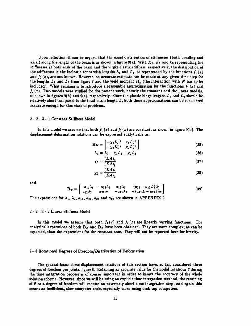
Upon reflection. it can be argued that the exact distribution of stiffnesses (both bending and axial) along the length of the beam is as shown in figure 9(a). With Kl. K2 and ko representing the stiff'nesses at both ends of the beam and the virgin elastic stiffness, respectively, the distribution of the stiff'nesses in the inelastic zones with lengths Ll and L2 • as represerlted by the functions h (x) and h (x), are not known. However, an accurate estimate can be made at any given time step for the lengths Lt and L2 from figure 7 and the yield moment AI" (the interaction with N has to be included). What remains is to introduce a reasonable approximation for the functions 11 (x) and h (x). Two models were studied for the present work. namely the constant and the linear models. as shown in figures 9(b) and 9(c), respectively. Since the plastic hinge lengths Ll and L2 should be relatively short compared to the total beam length L, both these approximations can be tOnsidered accurate enough for this class o( problems.

2 - 2 - 3 - 1 Constant Stiffness Model

In this model we assume that both h (x) and h (x) are constant. as shown in figure 9( b ). The displacement-deformation relations can be expressed analytically as;

and

B _ [-;\1L;I\:1L;I] N - -X2L;l X2L;l

L. = Lo + XtL) + X2L2 (EA)o

XI = (EAh

(EA)o X2 = (EAh

BT - [-at2~1 -a22~l a12..\l {a22 - a12L)..\l ] - all..\2 a21..\2 -all..\2 - (allL - a21)..\2

The expressions (or .\10 '\2, all, a22, an and a12 are shown in APPENDIX I.

2 - 2 . 3 - 2 Linear Stiffness Model

(35)

(36)

(37)

(38)

(39)

In this model we assume that both h (;t) and h (x) are linearly varying functions. The analytical expressions of both BN and BT have been obtained. They are more complex, as can be expected, than the expressions for the constant case. They will not be reported here for brevity.

2 - 3 Rotational Degrees of Freedom/Distribution of Deformation

The general beam force-displacement relations of this section have, 50 far. considered three degrees of freedom per joints, figure 6. Retaining an accurate value (or the nodal rotations (J during the time integration process is of course important in order to insure the accuracy of the whole solution scheme. However, since we will be using an explicit time integration method, the retaining of (J as a degree of freedom will require an extremely short time integration step. and again this means an inefficient, slow computer code, especially when using desk top computers.

11

It is possible to find an accurate solution to this apparant problem by studying the behavior of buildings during seismic motions. First we make use of the following two approximations:

i· No out of plane displacements for nodes within the floor under consideration. ii· Horizontal motions of all nodes within a floor are equal.

These a.te widely used (Anagn08topoul08, S.A., 1972 and Wilson, E.L., 1975) and acceptable assumptions for this class of problems. Following these assumptions, and defining the jt,. floor motions ~ Uj, "i and +j where:

Uj = horizontal floor displacement

Vj = vertical floor displacement at center of mass

+ j = floor rotation,

and using figure 10, the motions of the nodes within this floor can be expressed as:

Uij = Uj (40)

Vi; = Vj + +jTij (41)

the distance Tij is measured from the center of mass of the floor to the it" node, figure 10.

The relationship between the rotations 8ij and +j are more complex. It is possible to express 8ii as:

(Ji; = +j + fJii (42)

where fJij is the rela.xed nodal rotation, which results from three distinct sources:

i· Relative horizontal floor motions, figure l1(a). ii - Relative rotations of floors, figure UCb).

iii· Effects of rela.xed rotations of adjacent nodes (carryover effects, using the terminology of mo­ment distribution methodology). These effects are of secondary nature, especially for inelastic behavior of members and will be neglected.

Using figure 11 we define the elements of the matrix BT, equation 32. as B~" with t. = 1 ..• 4 indicating the element numbering with respect to the node. as shown in figure 11, m = 1,2, the row number, and n = 1 ... 4, the column number. The un'>alanced fixed end moment, M /' and the joint stiffness, 5" can be defined as:

and

T

5e = E5t t

51 = Bt, 52 = B~4 53 = B~l 54 = B~4

12

Uj+l

+j+l

Ui +j

Ui-l +i-I

(43)

(44)

the relaxed nodal rotation can the be expressed as:

(45)

Equations 40,41,42 and 45 completely define in an accurate manner the relations between nodal and floor displacements. It is possible now to write the equations of motion in terms of floor degrees of freedom, utilizing the larger time integration steps, then evaluate the nodal motions using the above equations.

2 - 4 Total Equations of Motion

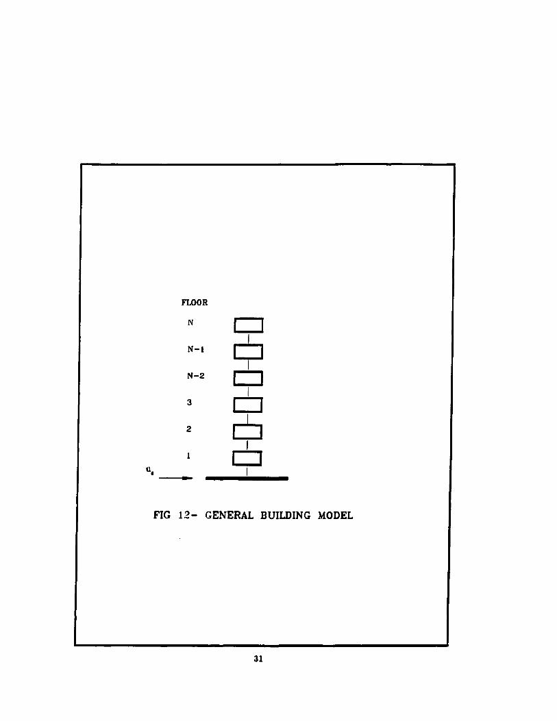
Consider the 20 mathematical model of a typical building with N floors, figure 12. Ea.c:h floor has 3 degrees of freedom as in figure 10. The equations of motion of this model is:

MU +CU + Fi = -MUg

M = Mass matrix

C = Damping matrix, proportional to mass

=AM U, U = Floor acceleration and displacements

F i = Internal force vector

ii, = Ground accelerations

I = Identity vector

(46)

(47)

The mass matrix is diagonal, for simplicity. The components of the matrix are the linear and rotational floor masses. The damping part of equation 46 is Rayleigh type damping [Clough, R.W. and Penzien, J., 1975). The parameter A can be adjusted so as to have the required fraction of critical damping at a. particular forcing frequency. The internal floor force vector, F i , can be • calculated from the internal forces of the individual element which intersect with the floor under consideration. Only columns (out of floor plane members) will have a contribution to this vector.

The marching time intergration algorithm can be established using the following finite differ­ence equations:

- -2 Uta = (~t) (U"H - 2U" + Uta-I) • -1

Uta = (~t) (U" - U,,-d,

which, when combined with equations 46 and 47 result in the time marching relation:

Equation 48 represent the main equation of this study. It links the nonlinear material "BOW" concepts, the integration along the length expressions and the distribution of deformations tech­niques, all in a simple, extremely fast yet accurate algorithm.

13

3 - "SNORT" COMPUTER CODE

3 - 1 General Description

The SNORT (Seismic NOnlinear Research Tool), computer code was written using the popular BASIC computer language. It was debugged using a desktop computer (an MSDOS machine, using a DOS version 3.30). The program implement aU the analytical features which were discussed in the previous chapters. In addition, it has the following features:

• It can handle for initial forces. A feature which is important for accounting for the coupling between the dynamic seismic effect!! and the static gravity loads in buildings, especially when the building materials a.re nonlinear.

• The program outputs both time histories of displacements and forces, as well as force-deformations relations of members.

• The input parameters are minimized through the use of floor information instead of nodal information. whenever possible.

The input to the program is arranged in a file named "TB.INP". A brief description of the input requirements follows.

3 - 2 Input to the Program

The following is a description of the input file "TB.INP". As we stated earlier, the program "SNORT" is written in BASIC. The input format is free form, with commas as the delimiters. The input line are:

READ IN MAIN:

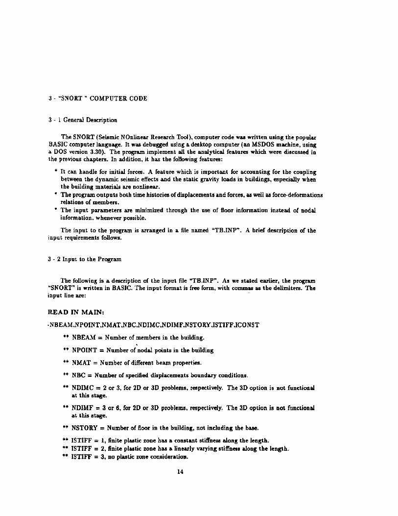
-NBEAM.NPOINT,NMAT,NBC,NDIMC,NDIMF.NSTORY,ISTIFF.ICONST

•• NBEAM = Number of members in the building .

•• NPOINT = Number of nodal points in the building

•• NMAT = N umber of different beam properties .

•• NBC = Number of !!pecified displacements boundary conditions .

•• NDIMC = 2 or 3, for 2D or 3D problems, respectively. The 3D option is not functional at this stage.

•• NDIMF = 3 or 6, for 2D or 3D problems. respectively. The 3D option is not functional at this stage .

•• NSTORY = Number of floor in the building, not including the base .

•• ISTIFF = 1, finite plastic zone has a constant stiffness along the length. •• ISTIFF = 2. finite plastic zone has a linearly varying stiffness along the length. •• ISTIFF = 3, DO plastic zone consideration.

14

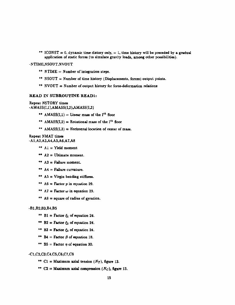
•• ICONST = 0, dynamic time distory only, = 1, time history will be preceded by a gradual application of static forces (to simulate gravity loads, among other possibilities).

-NTIME,NSOUT ,NVO UT

** NTIME = Number of integration steps.

** NSOUT = Number of time history (Displacements, forces) output points .

•• NVOUT = Number of output history for force-deformation relations

READ IN SUBROUTINE READ1:

Repeat NSTORY times -AMASS(I.1 ),AMASS(I,2 ),AMASS(I,3)

•• AMASS(I,I) = Linear mass of the It" floor

•• AMASS(I,2) = Rotational mass of the P" floor

•• AMASS(I,3) = Horizontal location of center of mass.

Repeat NMAT times ·A1,A2,A3,A4,A5,A6,A1,A8

•• A 1 = Yield moment

•• A2 = Ultimate moment.

•• A3 = Failure moment .

•• A4 = Failure curvature.

** AS = Virgin bending stiffness.

•• A6 = Factor p in equation 29 .

•• A7 = Factor w in equation 29.

•• AS = square of radius of gyration.

·81,82,83,84,85

•• Dl = Factor ~l of equation 24 .

•• D2 = Factor ~2 of equation 24.

•• 83 = Factor ~ of equation 24 .

•• B4 = Factor {J of equation 18.

•• 85 = Factor " of equation 30.

·C1,C2,C3,C4,C5,C6,C7,C8

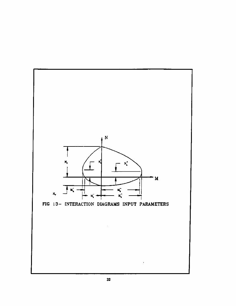
•• C1 = Maximum axial tension (NT), figure 13.

•• C2 = Maximum axial compression (N c), figure 13.

15

•• C3 = Uniaxial moment, +ve face in the interaction diagram, figure 13 .

•• C4 = Uniaxial moment. - t'e face in the interaction diagram, figure 13.

•• C5 = Balance moment, + ve face in the interaction diagram, figure 13.

•• C6 = Balance moment, - ve face in the interaction diagram. figure 13.

u C3 = Balance a.xial compression, +ve face in the interaction diagram, figure 13.

•• C3 = Balance axial compression, - ve face in the interaction diagram, figure 13.

Repeat NBEAM times

·IX(I.1 ),IX(I,2),IX(I,3),IMATNO

•• IX(I,l) = Node number of the start of the member .

•• IX(I,2) = Node number of the end of the member .

•• IX(I,3) = 0 or I, for beams or columns. respectively.

•• IMATNO = Material number of this member.

Repeat NPOINT times

.XCORD,YCORD,STORYNO

•• XCORD = Horizontal coordinate of this node .

•• YCORD = Vertical coordinate of this node .

•• STORYNO = Story number in which this node is located.

Repeat NBC times

·NODE.DOF

•• NODE = Node number where displacements are constrained .

•• DOF = Degree of freedom.

READ IN SUBROUTINE READ2:

If NSOUT > 0 otherwise, skip these lines

Repeat NSOUT

-LSO UTe 1,1 ),LSO UT(I,2),LSO UT(I,3 ),LSO UT(I,4)

•• LSOUT(I,l) = Node number (if LSOUT(I,3) is 2), or member number (if LSOUT(I,3) is 1) .

•• LSOUT(I,2) = Degree of freedom.

•• LSOUT(I,3) = 2 or 3, for displacement or force time histories, respectively.

16

•• LSOii"f(I,4, = 0 if LSOUT(I,3) is 2. For force time histories (LSOUT(I,3) is 1), input the required member end ( 1 or 2).

If NVO UT > 0 otherwise, skip these lines Repeat NVOUT

·LVQ UT(I,l ),LVQUT(i,'2),LVOUT(I,3)

.. LVOUT(I,I) = Member number .

•• LVOUT(I,2) = Degree offreedom, 1 for axial relations or 3 for moment-curvature relations .

•• LVOUT(I,3) = End of member, 1 or 2.

READ IN SUBROUTINE READ3:

-DT,DAMP,OMEGA,NTI

•• DT = Time integration step.

•• DAMP = Critical damping ration .

•• OMEGA = Forcing frequency at which DAMP is to be realized (HZ) .

•• NTI = Number of input a.cceleration steps. Note that NTI Ie NTIME.

If ICONST = 1 otherwise, skip these lines

-TC1,TC2,DAMPC

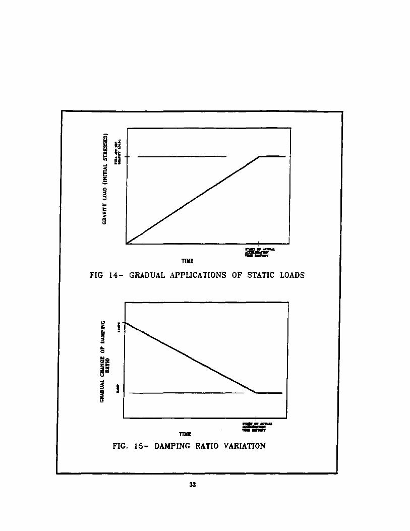
•• TC1 = Time of rise of static loads, figure 14.

•• TC2 = Time of duration of static loads, before the application of the dynamic loads, figure 14 .

•• DAMPC = Critical damping ratio at the start of the integration process, figure 15.

-LDlR(1),LDIR(2),LDIR(3)

•• LDIR( 1) = Ratio of floor mus which is applied as a static force in tbe I-direction.

•• LDIR(2) = Ratio of floor mus which is applied as a static force in tbe 2-direction .

•• LDIR(3) = Ratio of floor mus which is applied as a static force in tbe 3-direction.

Repeat NTI times -ACC(I)

•• ACC(I) = Acceleration time bistory, in "g" units.

3 - 3 Output Description

17

The output time histories are all written in a file named "TB.OUT". A complete description of the time history is included at the start of each time history. Post processing the output information should be fairly easy.

18

-l - RESULTS

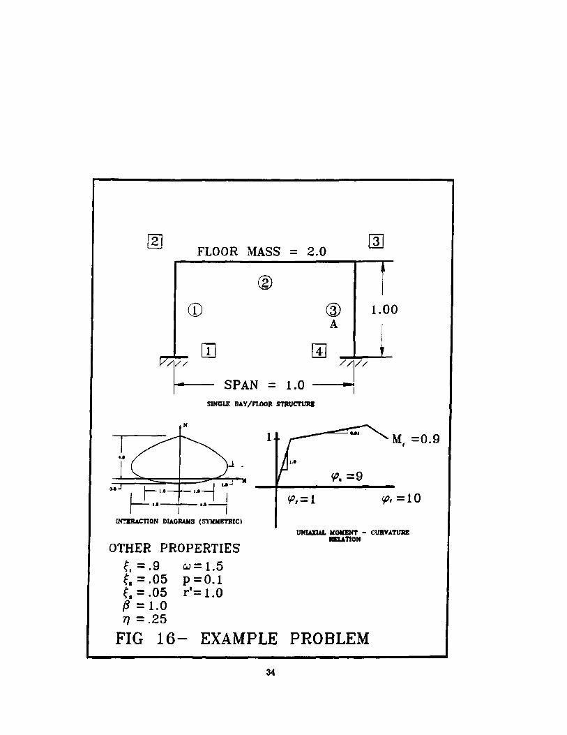
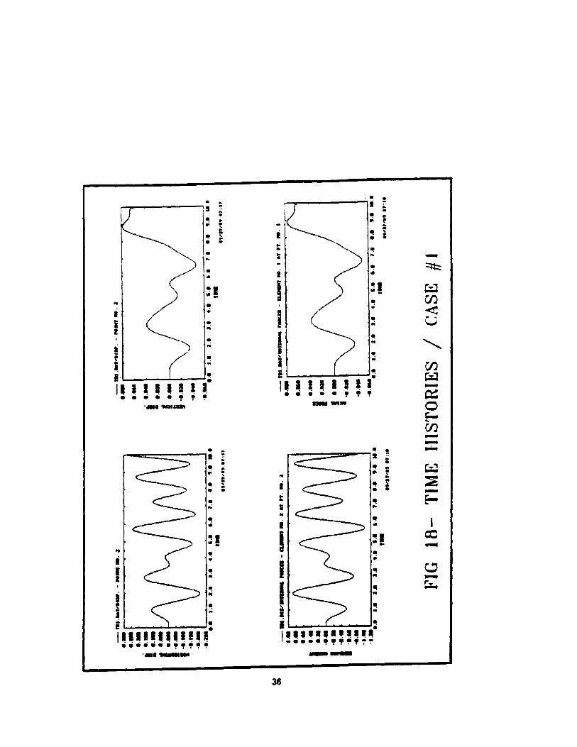
The program SNORT of the previous section was used to analyze a reinforced concrete frame subjected to a ground motion. Figure 16 shows the different parameters of the problem. The struc­ture itself is a single bay single story system. The base motion is applied at the two support points. The members of the structure were assumed to be identical and symmetrically reinforced, with their interaction diagrams, also shown, reflecting this symmetry. The uniaxial moment-curvature curve of the cross sections is also shown. The different parameters controlling shear reinforcements, strength and stiffness degradation are given in the same figure.

The base accelerations for this case are shown in figure 17. The vertical and horizontal acceler­ations have similar wave forms. The amplitudes of the two accelerations time histories are different. Two cases were considered. The first case (case I) we applied a factor of 0.75 to the horizontal wavE' form of figure 17 and a factor of 0 to the vertical vertical wave form. The second case (case II) w€ applied a factor of 0.75 to the horizontal wave form of figure 17 and a factor of 0.3 to the vertical vertical wave form. The choices of these factors reflect the desire to investigate the BOW model for conditions where the structural columns will be subjected to an almost uniaxial bending (case I), and a more realistic combinations of bending moments and axial forces (case II). It is also of importance to note that we decided to use an almost sine wave form with increasing amplitude for this study instead of a regular seismic wave form since the sine wave motions, because of its regularity, will be more suited to show the features of the BOW model than the irregular wave forms of the conventional seismic events. In addition, the purpose of this study is to investigate the different analytical techniques and the program's capabilities, rather than investigating specific structure subjected to a specific seismic motion. Based on these reasons, it was decided to use the wave forms of figure 17 for this study.

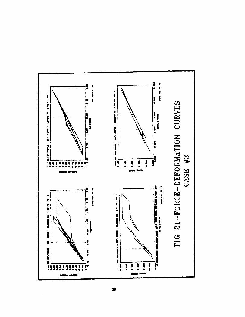
Figure 18 shows the displacements and forces at different locations in the structure and figure 19 shows some force deformation relations for two cross sections in the system for case 1. Figures 20 and 21 show similar information for case II. The axial force-axial strain curves of case I (figure 19) show an almost linear behavior. This is expected since the vertical deformations of the columns are due only to the overturning effects which are not Jargt' for a single story building. When we include a finite vertical acceleration, case II. figure 21. the nonlinear behavior of the axial direction becomes clear. A hysteric loop was formed in the axial force-axial strain curve of member number 1. Also the inclusion of the vertical accelerations has a clear reduction of strength in the moment-curvature curves. It is of interest to note that the yield moments changes during the motion in the moment curvature curves of figure 21. This is due to the coupling effects with the axial forces. Both of figures 19 and 21 show the different features of the BOW model such as degradation of strength and stiffness, coupling between axial forces and bending moments and crack opening and clcsing effects, among other things.

19

.5 - CONCLUSIONS

This Phase I resea.rch project had a general goal of the development of a method for treatment of RC buildings subjected to earthquakes. The resulting technique was to be accura.te for such structures a.nd easily usable by practicing engineers.

The specific objectives of Phase I were:

1. development of the methodology,

2. coding it in a computer program, and

3. making some computer runs to investigate both the program and the methodology.

We presented an innovative set of methods for treatment of RC structures which are subjected to seismic loads. The innovative methods addressed RC members on the cross sectional level, with the introduction of the BOW material model. We thel\ introduced a new simple and accurate method for integration along the length of the member. Finally the concept of distribution of deformation allowed us to retain the accuracy of joint rotations. without sacrificing the efficiency of calculations.

The computer code SNORT was prepa.red to perform these tasks. It was designed from ground up to run on desk top computers so that computational efficiency was essential, in addition to the accuracy of solution. Finally, some test runs were performed, and the different features of the new methodologies were observed and discussed.

To summarize, we have developed a theoretically sound, qualitatively effective yet efficient method for the nonlinea.r seismic analysis of RC buildings, and implemented it on a desk top computer. Making this kind of a tool accessible to practicing engineers, will certainly have a broad base of interest and commercial potential. Such a tool can be used for designing new RC structures, or investigating the safety existing buildings. In either application, it should be useful in construction, consulting engineering and architectural practices.

Possible Phase II program activities i- Generalization of the methodology, including the BOW model, the integration along the length

and the distribution of deformation, to three dimensional geometries. ii· Treatment of torsion, both on local element level, and on global structural level. iii- Addition of p-~ effects. iv- The user interface (input and output) of the program SNORT needs to be improved to be more

user friendly. Also the innards of the program can be changed to improve the calculational efficiency. Porting the program from the MS-DOS 3.3 operating system into the more capable OS/2 operating system will also be performed.

Acknowledgments This work was inspired by the many conversations we have had with P. Wei­dlinger. J. Baylor, I.Sandier and J. Wright provided many helpful suggestion during different stages of this study.

20

6 - REFERENCES

Anagnostopoulos, S. A., "Nonlinear Dynamic Response and Ductility Requirements of Building Structures Subjected to Earthquakes," Research Report Number R72-5., Civil Engineering Dept., Massachusetts Institute of Technology, Cambridge, MA, 1972.

Applied Technology Council, "Tentative Provisions for the Development of Seismic Regulatiofl8 for Buildings," ATC Publication, ATC-3, 1978.

Atkinson, G. M., "Implications of Eastern Ground Motion Characteristics for Seismic Hazard Assessment in Eastern North America," Proceedings, Conference on Earthquake Hazards and the Design of Constructed Facilities in the Eastern United States, sponsored by National Center of Earthquake Engineering research (NCEER) and New York Academy of Sciences (NYAS). Feb. 1988.

Baylor, J. and Wright, J., "Theoretical Background and User's Guide for the TRANAL Computer Program." Defense Nuclear Agency Report Number DNA-TR-87-212. Weidlinger Associates. New York. NY. July 1987.

Bieniek. M. P. and Funaro, J. R .. "Elaste-Plastic Behavior of Plates and Shells", Defence Nuciear Agency Report Number DNA-995iT, Weidlinger Assoc., New York, NY, March 1976.

Chung, Y.S., Meyer, C., Shlnozuka, M., "Seismic Damage Assessment of Reinforced Concrete Mem­bers," Technical Report NCEER-87-0022. National Center for Earthquake Engineering Research, State University of New York at Buffalo, Buffalo, NY, 1987.

Clough, R. W. and Johnston, S. B., "Effect of Stiffness Degradation on Earthquake Ductility Requirements," Procet!dings, Japan Earthquake Engineering Symposium, October 1966.

Clough, R. W. and Penzien, J., Dynamics of Structures, McGraw Hill Book Co., New York, 1975.

Hall, W., "Current Design Spectra: Background and Trends," Proceedings, Conference on Earth­quake Hazards and the Design of Constructed Facilities in the Eastern United States, sponsored by National Center of Earthquake Engineering research (NCEER) and New York Academy of Sciences (NYAS), Feb. 1988.

Levine. 11.5., "A Two Surface Plastic and Microcracking Model for Plain Concrete," Nonlinear Numerical Analysis of Reinforced Concrete. Winter Annual Meeting, ASME, Phoenix, AZ, Nov., 1982.

Martin, J. B., PltJ8ticity, The MIT Press, Cambridge, Mass., 1975.

Moehle, J. P., "Concrete Structures," Proceedings, Conference on Earthquake Hazards and the Design of Constructed Facilities in the Eastern United States, sponsored by National Center of Earthquake Engineering research (NCEER) and New York Academy of Sciences (NYAS), Feb. 1988.

Mould, J.C. and Levine, H.S., "A Three Invariant Viscoplastic Concrete Model," Proceeding" Second Interna.tional Conference on Constitutive Laws for Engineering Materials: Theory and Applications, Tucson, AZ, Jan., 1987.

Seeber, L., "Seismicity and Techtonics in the Eastern US," Proceedings, Conference on Earthquake Hazards and the Design of Constructed Facilities in the Eastern United States, sponsored by N a­tional Center of Earthquake Engineering research (NCEER) and New York Academy of Sciences (NYAS), Feb. 1988.

Somerville. P., "Earthquake Source and Ground Motion Characteristics in Eastern North America," Proceeding', Conference on Earthquake Hazards and the Design of Constructed Facilities in the

21

Eastern United States, sponsored by National Center of Earthquake Engineering research (N CEER) and New York Academy of Sciences (NYAS). Feb. 1988.

Uniform Building Code, "Earthquake Regulations," Chapter 23, Section 2312, 1985.

Wakabayashi, M, Design of Earthquake Resistant Buildings, McGraw-Hill, Inc., New York, NY, 1986.

Weidlinger, P. and Ettouney, M. M., "Seismic Behavior of High Rise RIC, Flat Plate Structures." Report to NCEER, National Center for Earthquake Engineering Research, BuffaJo, NY, 1988.

Wilson, E. L., "Three dimensional analysis of building systems (extended version)," Earthquake Engineering Reseo.rch Center Report No. EERC 75-13. University of California at Berkeley, April 1975.

Winter, G. and Nilson, A. H., Design of Reinforced Concrete Structures, McGra.w Hill Book Com­pany, New York, 1972.

22

APPENDIX I

EXPRESSIONS FOR DISPLACEMENT - DEFORMATIONS RELATIONS

U sing figure 9, define the following variables:

23

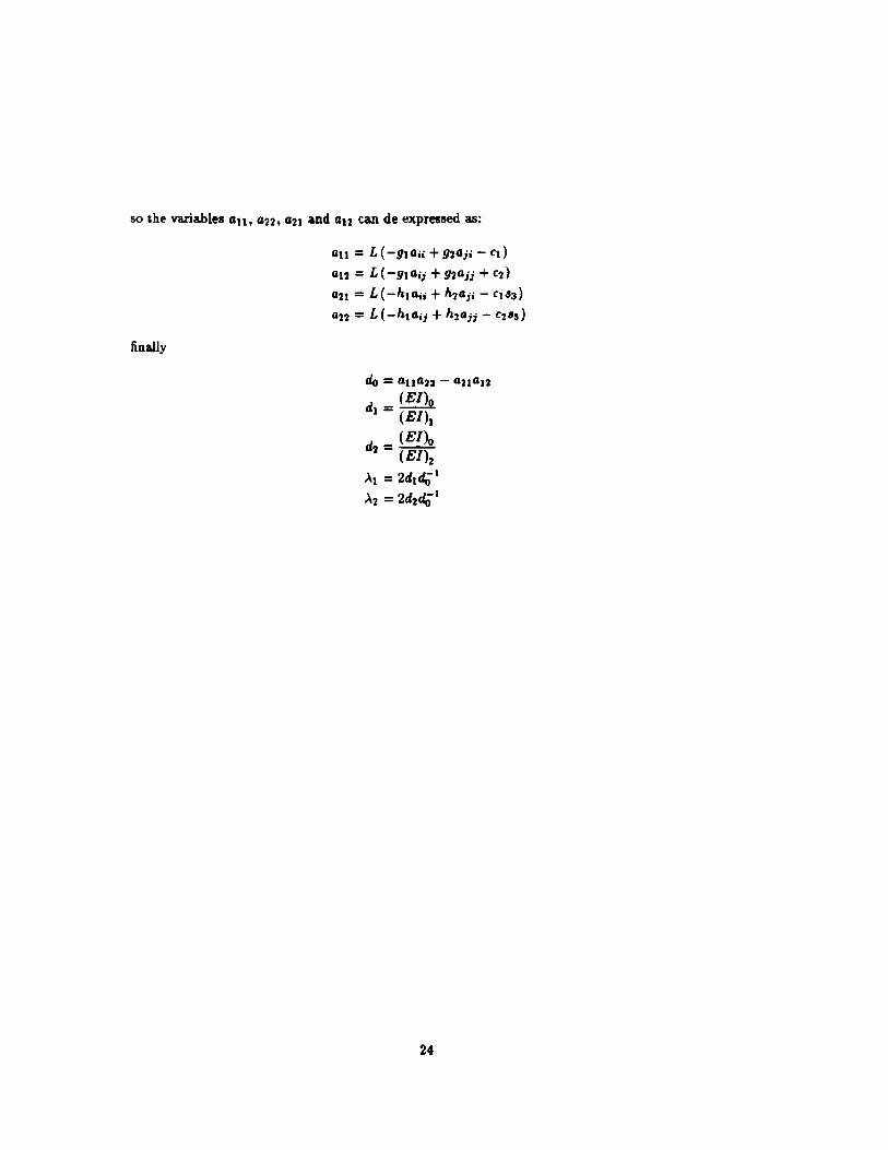
so the variables au, a22, a21 and au can de expressed as:

finally

an = L (-91 aii + 92aji - cd al2 = L(-9Iaij + 92 ajj + C2)

au = L (-hlaii + h2aji - CI"3)

a22 = L (-hi aii + h2ajj - C2"S)

do = I1Ua22 - a2l 1112

d _ (El)o I - (El)1

d (El)o 2 = (EI),

AI = 2dl dO l

A2 = 2d,dO l

24

FIG. 1- FORCES AND DEFORMATIONS OF 20 BEAM

N

FIG 2- YIELD CURVES( + / -) OF THE BO" MATERIAL MODEL

N

.- CURRINT V[EIJ) SURFACE

Ne

~ M

:::1 J M. NT

FIG 3- HARDENING PARAMETER IN THE BOW FORCE SPACE

26

M a

FIG 4- UNIAXIAL MOMENT - CURVATURE CURVE

M a

M 1

1'\1 FIG 5- FEATURES OF MOMENT - CURVATURE

RELATION

27

,Va ,VI

N,,~~

EI I I BENDING L-. __________ --". STIFFNESS

EA! I ~NESS

FIG 6- SINGLE ELEMENT APPROACH

~--------------~O

BENDING oc::::::::::::: MOMENT Y,

V=_V.=vJr--------------,j ~g:g

N=-NI=N( ~E FIG 7- INTERNAL FORCE DISTRIBUTION

END #1 END #2

FIG 8- MULTIPLE ELEMENT APPROACH

28

G~--------------------~ fJ!)

~~"I"I"!"I"!~~'I"I'!m"!"m~ ~

a- EXACT

~J

~--..II b-CONSTANT

K, J ~

c-UNEAR

~~ I

FIG 9- IMPROVED STIFFNESS DISTRIBUTION

29

..

---=~

'fl

FLOOR j-l

-I

FIG 10-FLOOR AND NODAL DISPLACEMENTS

a - DUE TO FLOOR DISPLACEMENTS

b - DUE TO FLOOR ROTATIONS

FIG 11- RELAXED NODAL ROTATIONS

30

FLOOR

N D I

N-l D I

N-2 D 3 6 2 ¢ 1 0

0. , .. FIG 12- GENERAL BUILDING MODEL

31

N

M

FIG 13- INTERACTION DIAGRAMS INPUT PARAMETERS

32

__ ACIUAL

"..- '11M ,..-

FIG 14- GRADUAL APPLICATIONS OF STATIC LOADS

~ I ::I c Q .. o

~2 ~5 y

... :! ! ~

FIG. 15- DAMPING RATIO VARIATION

33

~ FLOOR MASS 2.0 ~ -

© cD ® 1.00

A

~ W ~ Vr:-SPAN :: 1.0

~/ SINOLE BAY/FLOOR STRUCTURE

N

1N":'IRAcnON DIAGRAMS (SYMMETRIC)

OTHER PROPERTIES

t =,9 C!J=1.5 ~.=,05 p=O.l ~. = .05 rl= 1.0 p = 1.0 71 = .25

1 M, =0.9

<p. =9

~,= 1 <p, =10

UNIAXIAL MOMENT - CUJtVATURE RlLATlON

FIG 16- EXAMPLE PROBLEM

34

HORIZONTAL ACCELERATIONS c, UNIT'I)

&

3

2

.. I

~ 0

-1

-2

-3

-& 0 2 4 , • 10

,..(SIC)

VERTICAL ACCELERATIONS 0.4

(, UMTI)

O~

002

0.1 .. I

~ 0

-0.1

-002

~

-G.4 0 2 • • • 10

,..(SIC)

FIG 17- nMe HISTORY INPUTICASES STUDIED

• .. :

• i ,. .. J

. • • .. .. .. ~ ..

~ I .

I! I! ,

• • • I! ... ...

I! • • I .- -~I ! ~I ..... .....

.. II! , II! .. I ..

i .. II! I "! I

... '" • I II!

II .. ..

i / "!

• "! .. ·

i 'II! .. •

• e I-'I I • I • I I I I. I • • I • I • • • - • ,; ,

'" • • • • • , .; .;

. _.-- .... .....

--• • i !II

: ;

..... • III! .. .. .. • .. , .. I! i • •

~ • - • -II! t II! .. =

.. E-..

~ • I! • •

". I ..... " . .. .. .. i " I I!

• I

• I • II!

I ,.; ..

a • I " .; .. $ I! ~ I!

I .. I

.. i • i • I~ •• ~~' •• I~.~

.- .-I···~~···~··" .......•• ,., ...... ,.,.,~':' ._.--- --

36

:: II! :: ... .. .. • • N .. • ..

• i ~

I " II! .. .. • t ~ S t

N C • .. • to en

C C

N .. II .. ~

i • i -'I >-i -. I

• 0:: I III ~

.1 •• I

, ~

I I • .; III

a • - z , -. ,

I I II ~ -~ ,. -, , ~ .. ..

~ ~ <: e II! e • ::a -11I!1I!··~I11··~·I11~~ I~ II! II! II! II! II! II':' c:: =::;:t: ........... -- N - • - , ':'

I , • I I I I , --- to" mIIU 'WI_ 0

~ ~ ~ en

I Q ~

: U I • Ii I ..

i I : ~ " .. ,. .. - " i

,; " --II! • • : ~

,; to -• - c - • -. ~ .. • i - ~

I ~

i ! •• - II ! ~I I . •• ~

I I II I -

i ,

• • I ~ • I

I I , -

I II! I ~

'" I

, ..; I ~ I .. II I • • • I I I; = II! I ~ I! I! ~ ~ ~ II! ~ ~ • ~ I!':' • • • • • , , ,

-- ••••• '!t"'~ _'WI_

---37

• ~ • ~ I I .. .. • • II! t II! .. .. • t :; .. .. i II! : II! , • • t •

= N .. ~

? • i •

I ~ "'!I rn .... .. , II! < II! ..

i .. I u II! i ~

II! .. f

.. I • .......... ') • ) .;

l N

~ II! • • i .. r:n i i II! ~

i • • .. • I~ ! ! • I • I -I~ ! ! • • I ! ~ , , • • • • • ~ ~ • • • • • 0 ........ ... -- E-rn -• • • - -I !! Ii !! ...... .. ..

• •

< • • t .- t .. ~ .. N :; • ! i II! , ::: • •

~ II! r II! -,. .. • .. -c ..

N • i • I

I I II! I 0 .. ... N II! N i • .. I I 'II! C-' f

.. • I -II! c.:.. • .; ..

S II! II! I i .. i • i • .. • I~ ~ ~ I • I I ~ I~~S!~~~"~~~~ • • • • • '!'

, '!' ...... ,,""",,":''l' ... --- --38

• • .. !! .. .. - : • •

I c i i , .. ..

t I ,; I E ... ,. .. ; ,.

UJ c .. .. W i • i

•• ;> .. I ! -. •• Q:! ~ , .1 , .1 I I u , ,.

• • Z , I I 0

I • I .,. , -E-I I < ! I i I :e N

I··~~"·"~~··~ I~ ! I • I •• ;;;;t: .' ~ ·····"""':'i • • • • , , --- --- 0 C;;J '- r.n C;;J <

I Q U

~ . . I '.!

'.! N : i :

f i f ~ i • • .. U .. I • ,; .. i t S f"V ... i -.. ,. 0 c II . . i - '-i i ..

!I I i l I I .1 ....

I III I II N

I • I i' i ·11 i i '" ..... -I • I I r-.

I , ....

II • '!' • i • i I

I"II.~~~.~~~I!~ ,- • I I • I If -_ ..... ",,,-:- • • • Ii • , , --- -,..-

39