2

SAND2000-1256Unlimited ReleasePrinted May 2000

RADTRAN 5 Technical Manual

K. S. Neuhauser, F. L. Kanipe and R. F. WeinerTransportation Safety and Security Analysis Department

Sandia National LaboratoriesP.O. Box 5800

Albuquerque, New Mexico 87185-0718

ABSTRACTThis Technical Manual contains descriptions of the calculational models and mathematical andnumerical methods used in the RADTRAN 5 Computer Code for transportation risk andconsequence assessment. The RADTRAN 5 code combines user-supplied input data with valuesfrom an internal library of physical and radiological data to calculate the expected radiologicalconsequences and risks associated with the transportation of radioactive material. Radiologicalconsequences and risks are estimated with numerical models of exposure pathways, receptorpopulations, package behavior in accidents, and accident severity and probability.

3

Acknowledgements

The authors wish to acknowledge the contributions of Robert E. Luna and Jeremy Sprung, whocritically reviewed the manuscript, of David Chanin, who provided health effects data consistent withMACCS2, and of Mona Aragon, who created many of the graphics in this manual. The authorsalso wish to thank Jolene Manning and Patricia Tode for their secretarial assistance.

4

1 INTRODUCTION...................................................................................................................8

1.1 DEFINITION OF RISK...............................................................................................................81.2 CALCULATIONS PERFORMED IN RADTRAN 5.........................................................................9

1.2.1 Incident-Free Dose Calculation....................................................................................91.2.2 Accident Dose-Risk Calculation....................................................................................91.2.3 Other Calculations.....................................................................................................12

1.3 ORGANIZATION OF TECHNICAL MANUAL ....................................................................................12

2 SCOPE OF RADTRAN 5.....................................................................................................14

2.1 OVERVIEW OF RADIOACTIVE MATERIALS TRANSPORTATION.....................................................142.2 LIMITATIONS OF RADTRAN 5............................................................................................18

2.2.1 Fixed Facilities............................................................................................................182.2.2 Wind Direction...........................................................................................................182.2.3 Atmospheric Stability..................................................................................................192.2.4 Chronic Releases Cannot be Analyzed.......................................................................192.2.5 Chemical Hazards Cannot be Analyzed.....................................................................19

2.3 MATHEMATICAL SOLUTION STRATEGY...................................................................................192.4 RADTRAN 5 MODELS.......................................................................................................20

2.4.1 Package Models..........................................................................................................202.4.2 Transportation Models...............................................................................................212.4.3 Population Distribution Models.................................................................................232.4.4 Accident-Severity and Package-Behavior Models.......................................................242.4.5 Accident Probability Model.........................................................................................252.4.6 Meteorological Model.................................................................................................252.4.7 Exposure Pathways Models........................................................................................262.4.8 Health Effects Model...................................................................................................262.4.9 Non-Radiological Fatality Model................................................................................26

2.5 PRIMARY RADTRAN 5 CALCULATIONS ..............................................................................272.5.1 Incident-Free Transportation Dose Calculation........................................................272.5.2 Importance Analysis...................................................................................................272.5.3 Non-Radiological Fatalities........................................................................................272.5.4 In-Transit Individual Dose.........................................................................................272.5.5 Accident Risk Calculation...........................................................................................28

3 RADTRAN 5 ANALYSES OF TRANSPORTATION UNDER INCIDENT-FREECONDITIONS..............................................................................................................................29

3.1 INTRODUCTION TO INCIDENT-FREE TRANSPORTATION CALCULATIONS .......................................293.2 POPULATION DOSE FORMULATION.........................................................................................29

3.2.1 Gamma Radiation......................................................................................................293.2.2 Neutron Radiation......................................................................................................323.2.3 Summary of Final Expressions for Gamma and Neutron Radiation..........................34

3.3 DOSE TO MEMBERS OF THE PUBLIC........................................................................................363.3.1 Dose to Persons Along the Transport Link While the Shipment is Moving – Highway,Rail and Barge Modes.............................................................................................................363.3.2 Dose to Persons in Conveyances Sharing the Transport Link – Highway Modes.....423.3.3 Dose to Airline Passengers – Passenger-Air Mode...................................................46

3.4 DOSE TO POPULATION AT SHIPMENT STOPS – ALL MODES .......................................................473.4.1 Option 1 – Average-Distance Method........................................................................473.4.2 Option 2. Annular-Area Method................................................................................483.4.3 Use of Stop Model to Estimate Storage-Related Dose................................................49

3.5 DOSE TO WORKERS..............................................................................................................503.5.1 Dose to Crew Members – Highway and Air Modes...................................................503.5.2 Dose to Workers – Rail Mode....................................................................................513.5.3 Dose to Cargo Inspectors on Waterborne Vessels....................................................52

5

3.5.4 Dose to Flight Attendants – Passenger Air Mode.......................................................533.5.5 Dose to Handlers.......................................................................................................53

4 ATMOSPHERIC DISPERSION..........................................................................................56

4.1 BASIC PRINCIPLES OF ATMOSPHERIC DISPERSION...................................................................564.1.1 Atmospheric Dispersion Inputs to RADTRAN 5.........................................................584.1.2 Other Types of Dispersion.........................................................................................61

4.2 ATMOSPHERIC DISPERSION CALCULATIONS............................................................................634.2.1 General theory............................................................................................................63

4.3 RADTRAN CALCULATIONS................................................................................................684.3.1 Input Data..................................................................................................................684.3.2 First introduction of Vd ...............................................................................................684.3.3 Second introduction of Vd ...........................................................................................694.3.4 Amount of Material Deposited....................................................................................694.3.5 Calculation of IF.........................................................................................................69

5 CALCULATION OF ACCIDENT DOSES AND DOSE-RISKS....................................71

5.1 INTRODUCTION TO ACCIDENT CONSEQUENCE CALCULATIONS....................................................715.1.1 Exposure Pathways....................................................................................................715.1.2 Accident Severity and Package Response....................................................................715.1.3 Dose Calculation Outline...........................................................................................71

5.2 MATHEMATICAL MODEL FOR DOSE IN LOSS-OF-SHIELDING ACCIDENTS....................................725.2.1 LOS Gamma Dose for Small Packages.....................................................................735.2.2 LOS Neutron Dose for Small Packages.....................................................................745.2.3 Exposure Fraction (EF)..............................................................................................755.2.4 LOS Model Options for Type B Packages and Special Form Materials....................755.2.5 Exposure Times..........................................................................................................765.2.6 Early-Effects Calculation............................................................................................76

5.3 MATHEMATICAL MODELS FOR DOSE IN DISPERSION ACCIDENTS ..............................................785.3.1 Mathematical Model for Dose to an Individual from Inhalation of DispersedMaterials..................................................................................................................................785.3.2 Derivation of Mathematical Model for Integrated Population Dose from DirectInhalation of Dispersed Material.............................................................................................785.3.3 Derivation of Mathematical Models for Integrated Population Dose fromResuspension...........................................................................................................................805.3.4 Mathematical Model for Integrated Population Dose from Cloudshine.....................805.3.5 Mathematical Model for Integrated Population Dose from Groundshine..................81

5.4 ACTION LEVELS ...................................................................................................................845.5 CALCULATION OF DOSE FOR NO-ACTION DECISION.................................................................845.6 CALCULATION OF DOSE FOR EVACUATION AND CLEAN-UP .......................................................85

5.6.1 Ingestion Dose [optional]..........................................................................................865.7 ACCIDENT PROBABILITY AND DOSE-RISK...............................................................................86

5.7.1 Probabilities of Accidents...........................................................................................875.7.2 Dose-Risk for Loss-of-Shielding (LOS) Accidents......................................................875.7.3 Dose-Risk for Accidents with Dispersal.....................................................................875.7.4 Overall Dose-Risk from Dispersion...........................................................................89

6 HEALTH EFFECTS.............................................................................................................90

6.1 ACUTE HEALTH EFFECTS ......................................................................................................906.1.1 Mathematical Model for Number of Expected Early Fatalities and Early Morbiditiesfor Loss-of-Shielding (LOS) Accidents....................................................................................916.1.2 Mathematical Model for Number of Acute Health Effects from Inhalation ofDispersed Material..................................................................................................................96

6.2 LATENT HEALTH EFFECTS.....................................................................................................976.2.1 Calculation of Latent Cancer Fatalities and Genetic Effects for NondispersalAccidents..................................................................................................................................97

6

6.2.2 Calculation of Latent Cancer Fatalities and Genetic Effects for Dispersal Accidents986.3 TOTAL HEALTH RISK FROM ACCIDENTS................................................................................1006.4 EXPECTED NUMBER OF ACCIDENTS......................................................................................1016.5 IMPORTANCE ANALYSIS......................................................................................................1026.6 REGULATORY CHECKS........................................................................................................103

6.6.1 Exclusive-Use Designation.......................................................................................104

7 SPECIAL TOPICS..............................................................................................................107

7.1 RADTRAN 5 VALIDATION ...............................................................................................1077.1.1 Source Representation in Incident-Free Dose Calculations.....................................1077.1.2 Health Effects Conversion Factors...........................................................................1077.1.3 Package Behavior and Accident Probabilities..........................................................107

7.2 VERIFICATION AND SOFTWARE QUALITY ASSURANCE............................................................1077.3 NON-RADIOLOGICAL RISK - FATALITY RISK.........................................................................1087.4 RADDOG INPUT FILE GENERATOR ...................................................................................1087.5 GEOGRAPHICAL INFORMATION SYSTEM (GIS) DATA............................................................1087.6 LATIN HYPERCUBE SAMPLING (LHS) INTERFACE.................................................................1097.7 POPULATION RESIDENCE TIME.............................................................................................1097.8 ENVIRONMENTAL JUSTICE...................................................................................................110

8 LITERATURE CITED.......................................................................................................111

9 APPENDIX A - INDEX OF VARIABLES IN RADTRAN 5.........................................117

10 APPENDIX B- DERIVATION OF B FACTOR FOR RAIL TRANSPORTATION128

10.1 INTRODUCTION...................................................................................................................12910.2 CLASSIFICATION PROCEDURES ............................................................................................130

10.2.1 Shove-to-Rest FLAT..................................................................................................13010.2.2 Shove-to-Rest Low Hump.........................................................................................13010.2.3 Shove over Hump.....................................................................................................13010.2.4 Shove from Trim End...............................................................................................132

10.3 INSPECTION .......................................................................................................................13410.4 REPAIRS............................................................................................................................13510.5 CALCULATION OF B FACTORS ..............................................................................................137

10.5.1 General Freight (b1 – b7)..........................................................................................13710.5.2 B.5.2 Dedicated Rail (b8 – b11)................................................................................145

10.6 LITERATURE CITED.............................................................................................................147

7

8

1 INTRODUCTION

RADTRAN 5 is an ANSI FORTRAN 77 computer code for analysis of the consequences andrisks of radioactive-material (RAM) transportation. The first release of the RADTRAN code wasdeveloped by Sandia National Laboratories (SNL), under contract to the Nuclear RegulatoryCommission (NRC), as an analytical tool during preparation of the “Final Environmental Statementon the Transportation of Radioactive Material by Air and Other Modes" (NRC, 1977). The codewas subsequently modified to accept free-format data and issued as RADTRAN II (Taylor andDaniel, 1982). The Department of Energy (DOE) has sponsored development of the secondrelease and of all subsequent releases. With each release, the code's capabilities have been updatedand expanded (Taylor and Daniel, 1982; Madsen, Wilmot and Taylor, 1986; Neuhauser andKanipe, 1992).

RADTRAN 5 is to be used for the estimation of risks associated with incident-free transportationof RAM and with accidents that might occur during transportation. The U.S. Department ofTransportation (DOT) defines incident-free (or normal) transportation as “transportation duringwhich no accident, packaging, or handling abnormality or malevolent attack occurs.”1 ThisTechnical Manual describes the mathematical and numerical models used in RADTRAN 5. Thismanual is intended to be used with a companion document, the RADTRAN 5 User Guide(Neuhauser and Kanipe, 2000), which describes input data and RADTRAN 5 input and outputfiles. Throughout this document, bold italics identify important points.

All major modes of commercial transport may be analyzed with RADTRAN 5: highway, rail, barge,ship, cargo air, and passenger air.2 The NRC and the U.S. Department of Transportation (DOT)regulate carriage of RAM by all modes in the United States. Regulations promulgated by the NRCare primarily contained in the Code of Federal Regulations (CFR), specifically Title 10 CFR Parts71-73; regulations promulgated by the DOT are primarily contained in Title 49 CFR Parts171-178. These regulations establish maximum permissible package dose rates, maximumpermissible dose rates to vehicle crew members, exclusive-use shipment criteria, packagingcertification conditions and other features of radioactive materials transportation. Compliance withthese regulations of the package variables input by the user may be assessed with RADTRAN 5.

1.1 Definition of Risk

A common "shorthand" definition of risk is the product of consequence and probability. However,transportation risks, like the risks associated with carrying out any complex process, must bedecomposed into "what can happen . . ., how likely things are to happen . . ., and theconsequences for each set" of things that can happen (Helton, 1991). As the terminology in thisdescription implies, set theory provides an ideal framework for formal expressions of risk. "Whatcan happen" may be defined as disjoint sets of similar occurrences (Si, i = 1, ...nS) -- that is, eachset contains events with outcomes (consequences) that are similar. The sets are often scaled fromminimum to maximum consequence. "How likely things are to happen" can be defined as theprobability that an occurrence in set Si will take place; and "the consequences for each set" consist

1 Minor incidents (e.g. citation for improper placarding) and accidents below the reporting threshold may be excluded from

the statistical data. 49 CFR 225.5 and 49 CFR 390.5 both identify a fatality, an injury that requires medical treatment,and damage exceeding some calculated dollar amount as reasons an incident/accident must be reported. 49 CFR 171.15identifies evacuation of the public and transportation artery closure as additional reporting criteria. The radiologicalconsequence of a subthreshold event usually is limited to increased stop time.

2 Excludes minor modes such as horse-drawn vehicles, bicycles, motorcycles, air-cushion vehicles, etc.

9

of one or more specified consequence results (e.g., population dose) (Helton, 1991). One of thefirst steps in a risk analysis is definition of the sets of occurrences. In RADTRAN 5, this processis carried out separately for incident-free transportation and accidents. Since consequences mustbe calculated in order to calculate risk, RADTRAN 5 may also be used as for consequenceassessment.

RADTRAN 5 also may be used in conjunction with a Latin Hypercube Sampling (LHS) code toperform probabilistic risk assessments (PRAs). LHS is a structured-sampling method rather than arandom Monte Carlo method. In PRA applications, values of input variables are selected fromdistributions that represent the range of values that each variable may assume. The resultingoutputs (usually more than 50 and less than 500) may be displayed graphically as a CumulativeComplementary Density Function or CCDF, which is the method of choice for displaying riskresults. The subject of PRA is discussed further in Chapter 7.

1.2 Calculations Performed in RADTRAN 5

1.2.1 Incident-Free Dose Calculation

In calculations for incident-free transportation, the probability term is set equal to 1.0 even though itis actually equal to 1.0 minus the small probability of an accident. Thus, consequences rather thanrisks are calculated. In theory, the result could also be thought of as a dose-risk derived from arounded-off estimate of probability. However, if the incident-free value were added to the results ofthe appropriate accident dose-risk calculation (see Section 1.2.2), the sum would seldom appear tobe different from the incident-free value alone at the two- or even three-significant-digit level ofresolution. Thus, the two values always should be reported separately. The radiologicalconsequences of incident-free transportation are population doses of the various populationgroups that might be exposed to radioactivity from the package(s) being analyzed. Certainindividual doses are also calculated. RADTRAN 5 allows analysis of all population groupspotentially exposed during incident-free transportation (Table 1-1). The user selects only thosepopulations that are potentially involved for the problem under analysis and enters the requiredproblem-specific data. For example, population groups usually associated with incident-freemovement of a truck along a highway route-segment are:• persons beside the route (off-link population),• persons sharing the route (on-link population),• persons at stops, and• truck crewmembers.The magnitudes of the calculated doses depend on variables such as population density, distancetraveled, vehicle speed, and crew size. These variables are among those for which the user mustenter problem-specific values. The numerical models used to describe these sets of occurrences aredescribed in Chapter 3. The calculated doses for each population group are printed in the output. The printed results can have up to six significant digits, but this is a common artifact ofcomputational results in many codes and should not be interpreted to mean, for example, that smalldifferences in two results are significant. The unavoidable uncertainties in many input valuesclearly preclude such an assumption. It is strongly recommended that no more than twosignificant digits be used when reporting the results of a RADTRAN analysis.

1.2.2 Accident Dose-Risk Calculation

Dealing with Infinite Sets

10

In accident-risk analysis with RADTRAN 5, the analyst begins with the set of all accidents thatmight occur during the transportation event being analyzed and that might involve one or more ofthe RAM transportation conveyances being analyzed. This set and most of its subsets are infinitelylarge. In order to make the problem manageable (i.e., finite), the analyst must do several things. The first step is to remove highly improbable events (e.g., transportation vehicle struck bymeteorite) from consideration. This is generally accomplished by establishing a probability cut-off,and all risk analyses employ either an explicit or an implicit probability cut-off.

There are at least three methods of establishing a cut-off value. The most common method involvesthe use of historical statistics. To illustrate this method, consider the set of all possible accidents inwhich only a fender is dented. This set, like the set of all possible accidents of which it is a subset,is infinitely large. To reduce it to finite terms, five years of historical statistics on fender dentingmight be used to estimate the probability of such an accident. The historical data yield a set that canbe defined as the set of all previous transportation accidents in which only a fender is dented andthat are listed in the particular five years of historical data being used. When the number of suchaccidents is divided by the total vehicle-kilometers traveled in the same time period, the result is anestimate of the probability of occurrence of fender denting. This definition contains an implicit cut-off in that it excludes ways in which a fender could be dented that are so uncommon as to not haveoccurred in a five-year period. Events with probabilities of 10-12 to 10-13 per year or less usuallywould be excluded by this method.

Table 1-1- Potentially Exposed Population Groups by Mode

Truck Rail Ship & Barge AirPersons besidehighway

Persons besiderailroad

Persons besidewaterway (inlandwaterways only)

N/A

Persons sharinghighway

Passengers on passingtrains

usually N/A N/A

Public at stops Workers at railyards;public at other stops

Workers at ports Public and workers atairports

Truck crew Crew (at railyards andpullovers)

Ship or Barge crew Air crew; flightattendants

Handlers at intermodaltransfer

Handlers at intermodaltransfer

Handlers at intermodaltransfer

Handlers at intermodaltransfer

Interim storageworkers & public

Interim storageworkers & public

Interim storageworkers & public

Interim storageworkers & public

N/A N/A Passengers on vessel Passengers on airplaneInspectors atintermodal transfers,state borders, etc.

Inspectors at yards,intermodal transfers,state borders, etc.

Inspectors at ports,including intermodaltransfer

Inspectors at airports,including intermodaltransfer

A second means of establishing a cut-off value for RAM transportation accidents is the one-in-a-million criterion. For example, any scenario with an associated probability of inducing a latentcancer fatality less than one in a million per year (10-6 yr-1) might be excluded. This criterion hasbeen used in risk-based standards for benzene exposure, for example, promulgated by theEnvironmental Protection Agency (Cohrssen and Covello, 1989). The third method is to establishan explicit cut-off by excluding probabilities equal to or less than the probability of some rare but

11

catastrophic natural event such as the meteorite strike mentioned above (e.g., about 2E-18 peryear).3

An implicit cut-off established by historical statistics is the most commonly encountered type inaccident-risk assessment. Probability estimates derived from historical accident data always containan implicit cut-off in that they exclude types of accidents so rare as to never have appeared in thedata set. Clearly, the larger the data set used to estimate accident probabilities, the fewer rare eventsare excluded.

However, including rare events (especially classes of events that are so improbable that none has yetoccurred) has little effect on overall risk and consequence calculations. The reason for this is thatthe product of an extremely small probability and even a large consequence value is itself quitesmall. Transportation risk analyses performed by Sandia National Laboratories usually include oneor two such categories in order to extend the accident consequence categories somewhat beyondthose that can be predicted by historical data alone. This is routinely done for transportation riskanalyses that are included in an Environmental Impact Statement (EIS) or EnvironmentalAssessment (EA) prepared under the National Environmental Policy Act (NEPA) in order to ensurethat a full range of outcomes has been covered.

Accident-Severity CategoriesThe accidents remaining after application of a cut-off will still represent a wide range ofconsequences from little or none to quite severe. Therefore, they must be divided into new sets. Tosatisfy the “what can happen” criterion, each set must represent a logical grouping (accident-severity category) of accident outcomes.

Severity FractionsTo satisfy the “how likely is it” criterion, the overall probability of occurrence of an accident in aparticular severity category must be estimated. A two-step process does this:

1. The base probability (accident rate) is derived, usually from the historical record for each modebeing analyzed, although other methods are not excluded.

2. The base probability (accident rate) is multiplied in turn by the conditional probabilities(severity fractions) of the various accident-severity categories. Each product represents the totalprobability of occurrence of that accident-severity category. Severity fractions are usuallyderived by event-tree analysis although other methods are not excluded.

Radiological ConsequencesThere are two main types of radiological consequence: dispersion of contents and loss of shielding. Dispersion is analyzed in RADTRAN 5 with numerical models that represent:• package response(s) to particular accident environments;• form and nature of the direct radiation and/or the dispersed material that might escape a package

following a particular accident;• dispersion of any material released as airborne particulates or gases,• distribution and density of downwind population; and• exposure pathways via which released or dispersed material could cause human radiation doses.Loss-of-shielding is analyzed in RADTRAN 5 with numerical models that represent:• package contents as a source of radiation exposure;• strength of the source as a function of contents and shielding damage;• density of population in annular areas centered on the accident site.Consequences and probabilities are printed in the output.

3 Chapman (1998) estimates chance of a destructive (but not Extinction Level) impact at as much as 10-5 yr-1 for the earth as

a whole. The probability of striking any particular 100 m2 area (i.e., the vicinity of a loaded cask) is 100 m2 divided bythe earth’s surface area (5.1x10-14 m2) multiplied by 10-5 yr -1 , which is approximately equal to 2x10-18 per year)

12

Number of Significant Digits in OutputAs was noted in the discussion of incident-free results (Section 1.2.1), the number of significantdigits in the printed output cannot be taken as an indication of calculational accuracy. It is stronglyrecommended that no more than two significant digits be used when reporting the results of aRADTRAN analysis.

1.2.3 Other Calculations

In addition to the core capabilities discussed in the previous sections, RADTRAN has severaladditional features, some of which are automatically performed and some of which are optional. Among the former are the individual dose calculations. First, an individual dose for a person near atransportation route as shipments pass is calculated from user-defined input. Second, individualdoses for persons located at various distances downwind from dispersion accidents areautomatically calculated. One of the requested input values in the matrix of atmospheric dispersiondata is maximum downwind distance of each concentration isopleth, and individual doses, summedover all exposure pathways, are calculated as part of the population dose calculation. Theseindividual dose estimates are preserved, associated with the appropriate downwind distance, andreported in an output table. Finally, an importance analysis is automatically performed for incident-free dose calculations and printed in a table in the output. The total potentially exposed off-linkpopulation for multi-year shipping campaigns, in which migration is accounted for, also isautomatically calculated. The values are printed in a separate table in the output. The finalautomatic calculation produces a table of nonradiological accident fatalities, which is printed in theoutput. This calculation combines user-provided fatality rates and distances traveled to generatetotal fatality estimates.

RADTRAN 5 also permits an optional calculation of dose to persons downwind from a dispersionevent in which the user may enter separate population densities for each isopleth. Although theprimary outputs of RADTRAN 5 are dose and dose-risk estimates, health-effects risks may also becalculated as an alternative output option. Two separate runs of RADTRAN 5 are required toobtain results in terms of both dose and health effects.

1.3 Organization of Technical ManualChapter 2 of this Technical Manual describes the main component models in RADTRAN 5 and theprocesses and interactions represented by these component models. Chapters 3 through 5 describein detail the RADTRAN 5 computations of dose-consequences and dose-risks under incident-freeconditions and accident conditions. The equations used in RADTRAN 5 are given; each calculationand its contribution to the overall solution of the problem are discussed; and relationships withother operations in the RADTRAN 5 code are noted where necessary. Incident-free consequencemodels are discussed in Chapter 3; atmospheric dispersion is discussed in Chapter 4; and accidentdose-consequence models for dispersion and loss of shielding in Chapter 5.

The primary output of RADTRAN 5 is dose risk, and dose risk may be converted into health-effects risk either by offline calculation or by a second run of the code. Calculation of health-effectrisks is described in Chapter 6. Chapter 7 covers topics such as the user-friendly interface forgeneration of input files (RADDOG), the Latin Hypercube Sampling (LHS) method of performingprobabilistic risk analyses, non-standard applications of the code, and verification/validation. Appendix A contains a list of all variables in the equations in this manual and indicates theequations in which each variable appears. Appendix B describes the b variables used in railtransportation analysis.

13

14

2 SCOPE OF RADTRAN 5

2.1 Overview of Radioactive Materials Transportation

Transportation of radioactive materials (RAM) involves a wide range of events and operations.Transportation is not a goal in itself. We move a material from one location to another to servesome other purpose; e.g., a radiopharmaceutical may be transported from its point of origin to ahospital so that it can be used in a life-saving diagnostic procedure.

RAM must be shipped in packages that meet regulatory standards, and the radiation dose ratesoutside these packages must be calculated or measured and demonstrated to comply withestablished limits. Compliance of the package data that is input by the user with these regulatoryrequirements is assessed by RADTRAN 5. However, the code also allows the user to assess theconsequences of RAM transportation that fails to comply with regulations.

Seven modes of transportation are addressed in RADTRAN 5: two highway modes(tractor-trailer and light-duty vehicle), and rail, barge, ship, cargo air, and passenger airmodes. There are a variety of conveyances in each mode (e.g. ship mode includes break-bulkfreighters and container ships of a variety of tonnages) that may be used to transport RAM. Although not it is not entirely accurate usage in all cases, the term ‘vehicle’ is often usedinterchangeably with the term ‘conveyance.’ A shipment consists of one or more packages on asingle conveyance. A single conveyance may take a package directly from its origination point toits ultimate destination, or a package may be transported to its destination by more than oneconveyance and/or by one or more modes. RADTRAN 5 allows the user to analyze all modecombinations and associated conveyance changes (intermodal transfers). Crewmembers andinspectors may be exposed to the external radiation field around a package. If a package is shippedby more than one mode and/or conveyance, it will be handled during each transfer from oneconveyance to another and from one mode to another. Thus, package handlers are exposed notonly at route origins and destinations but also at transfer points. A package may be placed ininterim storage en route, and if so, warehouse personnel will also be exposed. Low levels of publicexposure will also occur.

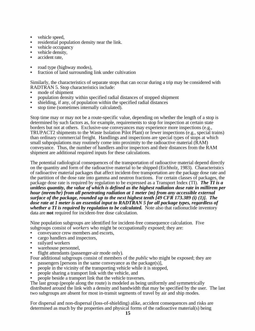
A package may be picked up or delivered to a freight forwarder and then consolidated with otherpackages into a single shipment. This single shipment may consist of packages obtained frommore than one shipper. The consolidated shipment may travel to a distribution point from which itmay be separated into individual packages that are delivered to more than one consignee. Handlingand warehouse storage can also occur during and between each of these transport phases as thepackages change modes or carriers. Figure 2-1 shows the various paths that a shipment mayundergo.

Since more than one mode may be used to transport a single package of radioactive material fromits point of origin to its final destination, RADTRAN allows each mode to be considered separatelyin assessing radiological impact. Parameters that have mode-dependent values, such as conveyancevelocity, package shielding, and population distribution, have different impacts on dose calculations. For further descriptions of general radioactive-materials transportation see Wolff (1984).

The characteristics of each segment (or link) of a transportation route may be considered withRADTRAN 5. These link characteristics include:• mode of shipment,• link length,

15

• vehicle speed,• residential population density near the link. • vehicle occupancy• vehicle density,• accident rate,

• road type (highway modes),• fraction of land surrounding link under cultivation

Similarly, the characteristics of separate stops that can occur during a trip may be considered withRADTRAN 5. Stop characteristics include:• mode of shipment• population density within specified radial distances of stopped shipment• shielding, if any, of population within the specified radial distances• stop time (sometimes internally calculated).

Stop time may or may not be a route-specific value, depending on whether the length of a stop isdetermined by such factors as, for example, requirements to stop for inspection at certain stateborders but not at others. Exclusive-use conveyances may experience more inspections (e.g.,TRUPACT2 shipments to the Waste Isolation Pilot Plant) or fewer inspections (e.g., special trains)than ordinary commercial freight. Handlings and inspections are special types of stops at whichsmall subpopulations may routinely come into proximity to the radioactive material (RAM)conveyance. Thus, the number of handlers and/or inspectors and their distances from the RAMshipment are additional required inputs for these calculations.

The potential radiological consequences of the transportation of radioactive material depend directlyon the quantity and form of the radioactive material to be shipped (Eichholz, 1983). Characteristicsof radioactive material packages that affect incident-free transportation are the package dose rate andthe partition of the dose rate into gamma and neutron fractions. For certain classes of packages, thepackage dose rate is required by regulation to be expressed as a Transport Index (TI). The TI is aunitless quantity, the value of which is defined as the highest radiation dose rate in millirem perhour (mrem/hr) from all penetrating radiation at 1 meter (m) from any accessible externalsurface of the package, rounded up to the next highest tenth [49 CFR 173.389 (i) (1)]. Thedose rate at 1 meter is an essential input to RADTRAN 5 for all package types, regardless ofwhether a TI is required by regulation to be calculated. Note also that radionuclide inventorydata are not required for incident-free dose calculation.

Nine population subgroups are identified for incident-free consequence calculation. Fivesubgroups consist of workers who might be occupationally exposed; they are:• conveyance crew members and escorts,• cargo handlers and inspectors,• railyard workers• warehouse personnel,• flight attendants (passenger-air mode only).Four additional subgroups consist of members of the public who might be exposed; they are• passengers [persons in the same conveyance as the package(s)],• people in the vicinity of the transporting vehicle while it is stopped,• people sharing a transport link with the vehicle, and• people beside a transport link that the vehicle traverses.The last group (people along the route) is modeled as being uniformly and symmetricallydistributed around the link with a density and bandwidth that may be specified by the user. The lasttwo subgroups are absent for most in-transit segments of travel by air and ship modes.

For dispersal and non-dispersal (loss-of-shielding) alike, accident consequences and risks aredetermined as much by the properties and physical forms of the radioactive material(s) being

16

transported and the specific radionuclides they contain as by the overall activity level of thematerials. Other factors that affect consequence and risk are accident probability, accident severity,package response, and dispersion environment. With RADTRAN 5, the user identifies a packagein terms of both its external dose rate and its contents (radionuclide inventory).

17

Figure 2-1. Possible Transportation Paths

18

To calculate transportation accident risks, the consequences and probabilities of vehicular accidentsmust be calculated separately and then multiplied by each other. The radiological consequences ofan accident are the potential doses (or health effects) that might occur as a result of:• dispersion of a specified quantity of radioactive material released from a compromised package,and/or• direct exposure of persons to ionizing radiation following damage to package shielding (loss ofshielding). The probability of occurrence of an accident in which radioactive material is released and/orshielding is damaged is determined from:(1) the expected frequency of all accidents and(2) the conditional probabilities of occurrence of accidents that are severe enough to result in one

ore more specified levels of damage to package integrity and/or shielding. A conditional probability is the probability, given that an accident occurs, that it will be of aspecified severity. As noted in Chapter 1, the expected frequencies of accidents by mode and routesegment are usually estimated from historical data and the conditional probabilities are usuallyderived from event trees. Up to 30 accident-severity categories may be defined for analysis withRADTRAN 5; each category must be assigned a conditional probability. Conditional probabilitiesdo not depend on the properties of the package; instead they depend on the conveyance type andtransportation mode. Package-response data (e.g., release fractions by accident-severity category)which are package-dependent are used to calculate consequences. The latter values are project-specific and must be provided by the user.

2.2 Limitations of RADTRAN 5

2.2.1 Fixed FacilitiesRADTRAN 5 is not intended for the performance of detailed location-specific consequence or riskanalyses such as are used for fixed facilities. In a location-specific analysis, the consequences andrisks associated with events or operations at a single specified location are calculated with apopulation distribution, wind roses and other weather data, etc. that are known. Nuclear powerreactors are examples of fixed facilities for which radiological risk assessments are performed. Computer codes such as MACCS2 (Chanin and Young, 1998a) are used to analyze fixed facilities. These codes require detailed weather and population data as input; such data are obtained in mostcases during the impact-analysis phase of site development. Weather data of a high level ofresolution are not available for most of the rest of the United States, including most segmentsof most highways, railroads, sea-lanes, etc.

Many of the analytical methodologies in RADTRAN differ mathematically from those used withfixed locations. RADTRAN is intended to analyze a radiation source (e.g., a RAM package)moving through a constantly varying landscape (i.e., traversing a route) in which the exact locationof any specific accident that might occur while the source is in transit cannot be known. Indeed, thenumber of possible locations of an accident is extremely large and cannot be predicted in advance. This uncertainty as to accident location sharply differentiates transportation risk analysis fromfixed-facilities risk analysis, where the landscape is invariant.

2.2.2 Wind DirectionEach route segment may be assigned a distinct population density, as noted in Section 2.1. Theassigned density is modeled in RADTRAN 5 as being uniformly distributed. In codes foranalysis of fixed locations, wind-direction data (wind roses) from weather stations are generallyused; these codes permit the analyst to calculate population exposures for each population thatmight be downwind at the time of an accident at the fixed site. However, weather stations are absenton most transportation routes, and, thus, wind-direction probabilities are unknown for most links.

19

The basic RADTRAN 5 calculational strategy for dispersal intentionally precludes the need forsuch unobtainable data by modeling the population as uniformly distributed.

A new feature of RADTRAN 5 allows non-uniform population-density data to be entered under thekeyword ISOPLETHP. The ISOPLETHP tool is useful for risk analysis only in special cases. However, it is highly useful as an analytical tool. For example, Mills and Neuhauser (1999b) usedISOPLETHP to compare the results of the approach to population modeling used in RADTRAN 5(densities uniform along each route segment) to that used in fixed-site codes (location-specificdensities by isopleth area). They confirmed that the two methods yield comparable results for across-country route.

2.2.3 Atmospheric StabilityAtmospheric-stability is a term that is used to describe the degree of turbulence and, hence, ofdilution during downwind transport in the atmosphere; it is discussed in Chapter 4. Like wind-rosedata, atmospheric-stability data and associated wind speeds are only available from fixedlocations with weather stations. Collection of data at a few such locations and extrapolation of theresults to other points in the surrounding region may be ultimately possible (so-called "mesoscale"weather), but consistently reliable methods of doing this are not yet available. National-averageatmospheric-stability data may be used (Church and Luna, 1974). A limitation of this approach isthat national-average data are not recommended for short routes. An alternative approach is the useof a single moderately conservative stability category and wind speed. See Chapter 4 for a detaileddiscussion of atmospheric dispersion.

2.2.4 Chronic Releases Cannot be AnalyzedChronic releases are often modeled in computer codes for the analysis of operations at fixedfacilities. Releases of this type cannot be analyzed with RADTRAN 5. Dispersal data enteredinto RADTRAN 5 must be for an instantaneous or “puff” release . Releases that might occurover a period of a few seconds up to a few tens of minutes are considered to be “instantaneous”for purposes of this analysis; nearly all transportation-related releases would fall into this category. The so-called Briggs equations (see Wark and Warner, 1981, Chapters 4 and 5) which modelreleases as point releases, yield erroneously high values at short downwind distances when appliedto “puff” releases. See Chapter 4 for a detailed discussion of atmospheric dispersion as modeledin RADTRAN 5.

2.2.5 Chemical Hazards Cannot be AnalyzedChemical-hazards analyses necessary to an assessment of the nonradiological consequences andrisks of shipping hazardous substances such as uranium hexafluoride are not included inRADTRAN 5.

2.3 Mathematical Solution StrategyRADTRAN 5 uses FORTRAN intrinsic functions for simple math and algebra as well asFORTRAN functions EXP, ALOG, AMIN1, and SQRT to solve mathematical equations. TheSandia Math Library (SLATEC) routines used in RADTRAN 5 are SSORT, BSKIN, BESK0,BESK1, E1, and AVINT. Additional SLATEC routines are called in RADTRAN 5 because they, inturn, are called from the five routines listed above. The FORTRAN intrinsic functions are widelyused and accepted as correct. The SLATEC routines are quality-assured solutions of variousmathematical functions and are electronically available through the NetLib website maintained byAT&T Bell Laboratories and others (www.netlib.org/slatec)

The calculational sequence of the RADTRAN 5 Computer Code is shown in Figure 2.2. Theoutside box represents the first stage of RADTRAN 5 calculations; the second box represents the

20

second stage, and so forth. The internal boxes represent the calculations RADTRAN 5 performs. They interact with the two outer boxes that supply input from the data file to produce the printedRADTRAN 5 output.

2.4 RADTRAN 5 Models

RADTRAN 5 contains nine sets of models that are used to estimate radiological consequences andrisks of radioactive material transportation. Figure 2-2 shows which models are used inincident-free and accident calculations and their relationship to each other. Variable values for thecomponent models come from user-supplied data and from internally calculated values. Theincident-free calculational sequence produces expected values of population dose with the Package,Population Distribution, and Transportation models. Similar models are used to calculate doses foraccidents involving only loss of shielding. RADTRAN 5 produces expected values of populationdose for accidents that result in dispersal by means of the Package, Transportation, PopulationDistribution, Accident-Severity, Package-behavior, and Meteorological models. The followingsections briefly summarize these models.

2.4.1 Package Models

Point- and Line-Source Models for Incident-Free Transportation

The formulation for estimating incident-free population dose from external radiation emitted bypackage(s) of radioactive materials in most cases is based on an expression for dose rate as afunction of distance from an isotropic point source of radiation (NRC, 1977). An isotropic pointsource is defined as a dimensionless source that emits radiation in all directions with equalmagnitude. For such a source, dose rate is inversely proportional to the square of the radialdistance from the source. A point-source model yields values of dose rates that agree well withactual dose rates measured at source-to-receptor distances greater than twice the characteristicpackage dimension (usually equivalent to twice the largest package dimension).

For larger packages, at exposure distances less than twice the largest package dimension, anisotropic line-source approximation is preferred. An isotropic line source is defined as aone-dimensional source that emits radiation uniformly in all radial directions along its entire length. For such a source, dose rate is inversely proportional to the distance from the source (rather thanthe square of the distance, as is the case for a point-source formulation).

Package Model: Isotopic Makeup and Properties of Package Contents

The Package Model also addresses the material(s) in the package(s) being analyzed and its (their)constituent radionuclides. These input data are used in the estimation of accident consequences. The variables for which input values must be supplied for each radionuclide in a package are:

• total number of curies per package (Ci);• average total photon energy per disintegration (MeV);• rate at which aerosol material is deposited on the ground (deposition velocity) (m/s);• cloudshine dose factors (dose factor for immersion in a cloud of dispersed material)

(rem-m3/Ci-sec);• physical characteristics (e.g., lung clearance time, which is dependent on particle size);• half-life (days); and• measures of the radiotoxicity of dispersed material (rem/Ci inhaled, etc.).

21

The internal radionuclide data library in RADTRAN 5 supplies all of the listed values except thefirst (number of curies) for all commonly shipped radionuclides. The user may use the DEFINEfunction of RADTRAN 5 to define additional radionuclides should that be necessary.

2.4.2 Transportation Models

The Transportation Models define those properties and characteristics of the transportationinfrastructure that influence the calculation of incident-free dose, accident consequences, andaccident probabilities. The two main divisions are route-segments and stops.

Route-Segment Model (LINK)

RADTRAN 5 allows separate treatment of each segment or link of a transportation route with theLINK subroutine. The LINK subroutine is a powerful analytical tool in RADTRAN 5 for analysisof route-related transportation risk factors. LINK allows the user to subdivide all or any part of aroute into a maximum of 60 separate route segments (or segment aggregates). LINK also can beused to analyze the same route segment(s) in a variety of conditions

22

Figure 2-2. RADTRAN 5 Component Models and their Interrelationships

23

such as daytime and nighttime population densities (Mills and Neuhauser, 1999a), rush hour andnon-rush-hour traffic conditions, and current and projected population densities.

The user must provide four types of input data:• link length in kilometers;• traffic-pattern data;• shipment data;• accident-rate data.Traffic-pattern data include such factors as traffic density and vehicle occupancy. Shipment datainclude the number of shipments, the number of crew and passengers, if any, occupying the RAMtransportation conveyance, the distance between the crew and the nearest package(s), etc. The firstthree categories of data are used for incident-free calculations as described in Chapter 3. The firstand fourth categories (link length and accident rate (accidents/vehicle-km)) are multiplied byuser-defined conditional probabilities of occurrence for accident-severity categories to generate amatrix of accident probabilities, as described in Chapter 5.

Stop Model (STOP LINK)

RADTRAN 5 contains a subroutine analogous to the LINK subroutine that combines user-provided data to calculate stop-related doses. The term “stop” is applied to instances in which avehicle carrying RAM is stationary with respect to its surroundings. If known, informationabout each stop may be entered as individual stop-links. Multiple stops of like nature (e.g.,refueling stops during highway-mode transportation) also may be aggregated. When stops areaggregated, total stop time and average or typical properties of the aggregated stops should be usedas input values. Since the exact location of refueling and rest stops usually cannot be predicted inadvance, the aggregation method is often used for these types of stops. Other types of stopsinclude inspections (e.g., at state or national borders), intermodal transfers, classification inrailyards, and short-term storage while en-route. The potentially exposed populations associatedwith these various types of stops are discussed in Section 2.3.3. In all cases, however, the userdefines one or more STOP LINKs and enters information on (1) the duration of each stop (or theaggregated stop time), (2) the number or density of potentially exposed persons, and (3) theirlocation relative to the location of the stopped shipment. The latter options are discussed in Section2.4.3.

2.4.3 Population Distribution Models

There are several distinct populations that may be exposed during incident-free transportation. People residing adjacent to a link are collectively referred to as the off-link population, a termcoined by the original developers of RADTRAN. This population is modeled as being uniformlydistributed on an infinite flat plane at some user-defined density. Each route segment must beassigned a population density, even though it may be zero as in the case of maritime travel on theopen seas.

For overland modes, up to three separate subpopulations may share the transport link. Collectivelyreferred to by the original developers of RADTRAN as the on-link population, they are separatelymodeled. The subgroups are:• persons in vehicles traveling in the same direction as the transport vehicle,• persons in vehicles traveling in the opposite direction, and• persons in vehicles travelling in the same direction as the transport vehicle that pass that vehicle

(highway modes only). The first two subgroups are modeled as each occupying a single lane, which is treated as an infinitestraight line along the length of which vehicles are uniformly spaced in both directions. Thespacing is determined by user-supplied vehicle-density and velocity data. The third on-link

24

subpopulation is addressed in the passing-vehicles model. In this model, persons in vehiclesoccupy the space in adjacent traffic lanes where vehicles reside while passing; a further condition ofthe passing-vehicles model is that the space is always filled by a vehicle for the duration of the trip,but not always by the same vehicle. The number of persons per vehicle is a user-defined variable. The calculated dose represents a conservative population-dose estimate rather than a dose to anindividual. It is conservative because the passing space in the real world is not always occupied.

Members of the public who may be present at stops make up a separate population subgroup. Dose to this subgroup is modeled in one of two ways (1) as a specific number of persons located ata given distance from a stationary source for a specified amount of time or (2) as a populationdensity located within an annular area for a specified amount of time.

Handlers and inspectors who may work in close proximity to a package are included in aseparate population model. For large packages, these close-proximity doses are estimated with aline-source model. For the crewmember subgroup, the number of crewmembers, their distancesfrom the package(s), and the nature of intervening shielding (if any) are user-definable, but theduration of exposure is calculated internally from speed and distance parameters. Finally, en-routestorage, if any, is treated as an ordinary stop, and dose to warehouse personnel is calculated withthe same model as public stop dose.

2.4.4 Accident-Severity and Package-Behavior Models

The Accident-Severity Model allows the user to assign all accidents to a maximum of 30 user-definable severity categories. The category definitions should be based on quantitative estimates ofthe forces potentially applied to package(s) during accidents and on the loss of shielding and/orrelease of radioactive species that may occur in response to these forces. The latter are referred toas release fractions. For loss-of-shielding situations, the analog to the "release fraction" is thefractional degradation of package shielding rather than actual release of contents. The categoriesshould be clearly related to the set of fire, crush, impact, and puncture forces encountered inaccidents and simulated in package-certification tests; however, unusual or specific abnormalenvironments associated with the problem being analyzed may be included as distinct categories. Several categorization schemes have been developed for spent fuel casks and other Type Bpackagings:• 6 categories (Wilmot, 1981);• 8 categories (NRC, 1977);• 9 categories (Sprung et al., 1998)• 20 categories (Fischer et al., 1987).The preferred method of developing severity categories is event-tree analysis, which was used bythree of the four authors cited above. The user is not required to use 30 categories, and categoriesmay be aggregated or dis-aggregated as the needs of a problem dictate. However, the categorydefinitions must cover the range of possible accidents (after taking any probability cut-off intoaccount). In mathematical terms, the sum of the probabilities of occurrence (severity fractions)of all the categories defined by the analyst must be approximately 1.0. There is no necessaryrelationship between the number of categories and the range covered. All of the schemes citedabove cover approximately the same range of accidents. However, the 9-category Sprung et al.scheme covers one scenario (severe fire without impact) that is not explicitly covered in the 20-category Fischer et al. scheme.

The Package-Behavior Model combines user-specified package-release fractions with otheruser-defined values representing, respectively, the fraction of each nuclide that becomes airborneand the fraction of an airborne radioactive material that is of respirable size as a consequence ofinvolvement in an accident of a given severity. There must be a complete set of package-behaviordata for each accident-severity category defined by the user. RADTRAN 5 contains no defaultsnor are there any recommended values for these variables; their values must be assigned by the

25

user. Other variables, such as the deposition velocity of airborne particles of each released material(an indicator of particle size), which also are used in the calculation, have defaults or recommendedvalues, but they are subordinate to the main fractional release variables. The latter are combinedwith the accident probabilities for each severity category (see Section 2.4.5), the number ofpackages, and the number of trips to determine expected values of release of each material in eachlink. Sprung et al. (1998) gives values of all these variables in a 9-category scheme for a fewspecific materials (various types of research-reactor spent fuel).

2.4.5 Accident Probability Model

This section of the code is not so much a model as an array of input data that are combined bysimple multiplication. The data consist of (1) the base accident probabilities for a given mode andlink and (2) the conditional probabilities, given that an accident occurs in a given transportationmode, that it will be of a particular severity. These conditional probabilities are called severityfractions. The base-rate values usually are derived from published historical data, but are notrequired to be. Severity-fraction values must reflect the severity-category scheme selected ordeveloped by the user (see previous section). That is, a conditional probability must be associatedwith each severity category for each mode in the analysis. They should be developed concomitantlywith the development of the severity categories themselves, preferably by generation of one or moreevent trees, as recommended in Section 2.4.4. Probabilities of fatalities from all causes are enteredin a separate array; they also are developed from published sources and are used to generateestimates of non-radiological fatalities (see Section 2.4.8).

2.4.6 Meteorological Model

The dispersal of a cloud of aerosol debris potentially released at the site of a severe accident alsomust be described in order to estimate consequences. Basic dispersion calculations are notperformed within RADTRAN 5. Instead, the user must provide either a table of time-integratedconcentration (TIC) values, with corresponding downwind areas (isopleth areas) or fractionaloccurrences of Pasquill atmospheric stability categories A through F (Pasquill, 1961).

TIC and isopleth-area values may be generated by one of the puff models now available [e.g.,AIRDOS (Moore et al, 1979), CAP88 (Beres, 1990); CAP88-PC (Parks, 1992), INPUFF (Petersenand Lavdas, 1986), etc.]. The initial “puff” must have dimension; that is, it should not bemodeled as a point source. Doing the latter leads to false and excessively high concentrationestimates in the innermost downwind isopleths. However, in the absence of specific information, itis acceptably conservative to model a “puff” as having a small diameter. “Smokestack” plumemodels for chronic releases should NOT be used to generate isopleth areas or TIC values.

The user must enter the maximum downwind extent of each isopleth. RADTRAN 5 contains atabulation of national-average values for these variables. The national averages may be used in theabsence of other information and, in the United States, will generally yield acceptable results forroutes longer than 500 km (310 mi.) (Mills and Neuhauser, 2000). As was noted in Chapter 2, itmay not be desirable to employ these values for very short routes, especially routes of only a fewkilometers.

26

Tabulated time-integrated concentration and area values for conservatively selected wind speeds alsoare included within the RADTRAN 5 code for each Pasquill category as a convenience to the user;the user is not required to employ them. The values are conservative because they represent asmall-diameter (10 m) ground-level release and the lowest wind speed consistent with each stabilitycategory. Weighted averages of the individual atmospheric stability group results are calculated byRADTRAN 5 and printed in the output.

The Meteorological Model also calculates individual doses. The dose to an individual located onthe centerline at the maximum downwind extent of each isopleth is calculated as a step in thepopulation-dose calculation (see Figure 2-2), but the values were not saved in previous releases ofRADTRAN. These calculations were originally preserved by a separate code (TICLD) that nowhas been incorporated into RADTRAN 5 (Weiner, Neuhauser and Kanipe, 1993). Theseindividual-dose values are saved and printed in the output.

2.4.7 Exposure Pathways Models

In addition to the direct exposure that may be expected from loss-of-shielding scenarios,RADTRAN 5 models five exposure pathways associated with dispersal of material from damagedpackage(s). These pathways are:• inhalation• cloudshine• resuspension• groundshine• ingestion.Minor and/or uncommon pathways such as absorption through skin or through open wounds arenot included. The impact on delayed doses from resuspension and groundshine of post-accidentactions such as evacuation and clean-up activities may be accounted for with the ExposurePathways Model.

2.4.8 Health Effects Model

Most doses calculated in RADTRAN 5 are either effective dose equivalents (E.D.E.s) or committedeffective dose equivalents (C.E.D.E.s). Prompt doses (i.e., doses from short exposures to externalradiation) are expressed as E.D.E.s. All incident-free doses are of this type, as are certain types ofaccident-related exposures. Doses that occur over long periods of time, such as doses from inhaledor ingested radionuclides that are retained in the lungs or gastrointestinal tract or are translocated toother organs are expressed as C.E.D.E.s. Dose commitments are calculated for periods of 1 year(for potential early effects) and 50 years (for latent effects). E.D.E.s and C.E.D.E.s for individualsare expressed in units of rem (see glossary). Population E.D.E.s and C.E.D.E.s are expressed inunits of person-rem. Organ doses (in rem) also are computed for internal exposures via theinhalation and ingestion pathways. In the Health-Effects Model, organ doses associated with thevarious exposure pathways are compared to dose thresholds for early mortality and morbidityderived from Evans et al. (1985). Latent effects (cancers and genetic effects) are calculated by useof published conversion factors (NAS/NRC, 1990). The “whole-body” doses (E.D.E. andC.E.D.E.) are used to estimate cancer incidence; gonad dose is used to estimate genetic effects infuture generations.

2.4.9 Non-Radiological Fatality Model

27

RADTRAN 5 contains a subroutine that calculates expected traffic fatalities from non-radiologicalcauses. These expected values are the products of published accident fatality rates (from theProbability Model) and user-specified input on distance traveled (from the Transportation Model). Unlike radiological exposures, non-radiological fatalities may occur even when the conveyance isempty. Thus, the one-way trip distance must doubled in the calculation of non-radiologicalfatalities to account for the return trip of the conveyance. In view of the extreme uncertaintiesnow known to be associated with particulate inhalation models, hypothetical fatalities from exposureto vehicle emissions are no longer estimated in RADTRAN.

2.5 Primary RADTRAN 5 Calculations

2.5.1 Incident-Free Transportation Dose Calculation

For analysis of incident-free conditions in RADTRAN 4, the package dose rate andpackaging-specific characteristics are used to model a package (or shipment) of radioactive materialas a modified point source and, for receptor distances less than two characteristic packagedimensions from large packages, as a line source. Characteristics of the transportation system arethen incorporated into mode-specific models, which use a set of input parameters to describe thepopulation along the route and at stops, and other critical mode-dependent characteristics such asvehicle velocity and stop duration. Population densities for each route segment must be defined bythe user, in addition to the characteristics of the various sub-populations that receive off-link,on-link, passenger, crew, stop, handling, and storage doses. The user-assigned values describingthese potentially exposed subgroups may be varied by mode and by population-density zone(urban, suburban, and rural). The user is given wide latitude in adjusting parameters for analysisfor a specific problem, but the quality and quantity of the available data will limit the accuracy of theresults.

2.5.2 Importance Analysis

Each incident-free consequence analysis performed by RADTRAN 5 is accompanied by animportance analysis, the results of which are printed in all forms of the output except the shortest(summary). This analysis uses partial derivatives as described in Chapter 6 to determine the effecton the overall result of a 1-% change in each input variable. The variables are listed in rank orderfrom the largest positive change to the largest negative change.

2.5.3 Non-Radiological Fatalities

Fatalities from all causes, estimated as described in Section 2.4, are printed in the output in aseparate table. These represent the deaths that would be expected to occur as a result of ordinarymechanical impacts. They include such categories as pedestrians struck by a vehicle, that result inone or more fatalities and exclude consequences associated with radiation exposure of any kindfrom hypothetical RAM package damage, which are calculated elsewhere in RADTRAN 5. Non-radiological fatalities are typically the largest fatality value calculated.

2.5.4 In-Transit Individual Dose

28

In a separate calculation, the dose to an individual located at some user-specified distance from ashipment traveling at some user-specified velocity is calculated with dose-rate data from thePackage Model. If the distance and velocity values are the smallest predicted for actualtransportation conditions, then this subroutine will calculate a maximum or bounding value ofindividual dose.

2.5.5 Accident Risk Calculation

The accident module combines user-supplied data on packaging behavior (release fractions, etc.)and accident severity to assess radiological consequences (population doses) for accidents ofvarying severity. Separate calculations are performed for each accident-severity category in eachpopulation-density zone. The consequence value is multiplied by an appropriate probability ofoccurrence derived from historical accident data to give a risk value; the sum of these individual riskcalculations weighted by segment length is the total radiological accident risk. To performconsequence calculations for release accidents, dispersal from the release point (hypotheticalaccident site) to downwind deposition areas is calculated either with Pasquill atmospheric-stabilityclasses A through F or with user-defined values for time-integrated concentrations (TICs). Consequences associated with the six exposure-pathways models (i.e., direct exposure, inhalation,cloudshine, resuspension, groundshine, and ingestion) are calculated separately and summed.

29

3 RADTRAN 5 ANALYSES OF TRANSPORTATIONUNDER INCIDENT-FREE CONDITIONS

3.1 Introduction to Incident-Free Transportation CalculationsRADTRAN 5 calculates the expected population doses or health effects, as the userchooses, for specific population groups and performs and importance analysis for each linkof the route(s) under analysis. The population groups include the following:• Off-link population• On-link population• Population in the vicinity of stops• Conveyance passengers• Transportation workers• Package handlers.

Under keyword LINK, each route segment must be designated as rural, suburban, or urbanin character. This character designation is usually based on population density, although itis not required to be. Doses are given on a link by link basis in the output along with rural,suburban, and urban subtotals. Total population doses as well as individual in-transit dosesare calculated.

The importance analysis for incident-free transportation shows the increase or decrease thatevery variable causes in the outcome of RADTRAN 5 calculations if the input variable valueis increased by one percent (see Chapter 6). Results are presented in tabular form in theoutput.

3.2 Population Dose Formulation

3.2.1 Gamma RadiationThe formulation used to assess population gamma dose during incident-free transportationis based on an expression for gamma dose rate as a function of distance from an isotropicpoint source (i.e., a source emitting gamma radiation in all directions with equal magnitude)(AEC, 1972). Reflection/absorption by the ground surface is neglected in this model. InRADTRAN 5, this type of point-source approximation is used to represent an individualpackage, shipment, or conveyance. In the absence of data allowing the specification of aneutron component of dose rate, the user should treat the entire dose rate as gammaradiation. Modifications that permit separation of the dose rate into gamma and neutroncomponents are discussed in the next section. Because neutrons are rapidly attenuated inair, the all-gamma treatment gives a slightly conservative estimate of overall population dose.

The formulation given here treats the package or shipment dose-rates as if they were 100%gamma radiation. The gamma dose-rate formula for an isotropically radiating point-source(AEC, 1972) is given by

C r)B( r)exp(-r 4

S (r)DR

2

photong ⋅⋅⋅=

(1)

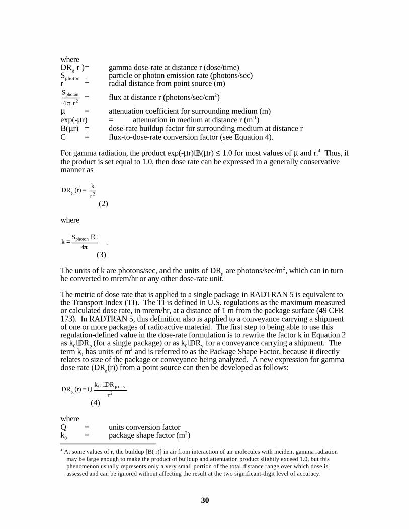
30

whereDRg r )= gamma dose-rate at distance r (dose/time)Sphoton = particle or photon emission rate (photons/sec)r = radial distance from point source (m)

2

photon

r 4

S= flux at distance r (photons/sec/cm2)

µ = attenuation coefficient for surrounding medium (m)exp(-µr) = attenuation in medium at distance r (m-1)B(µr) = dose-rate buildup factor for surrounding medium at distance rC = flux-to-dose-rate conversion factor (see Equation 4).

For gamma radiation, the product exp(-µr)⋅B(µr) ≤ 1.0 for most values of µ and r.4 Thus, ifthe product is set equal to 1.0, then dose rate can be expressed in a generally conservativemanner as

2gr

k (r)DR =

(2)

where

4

CS k photon ⋅

= .

(3)

The units of k are photons/sec, and the units of DRg are photons/sec/m2, which can in turnbe converted to mrem/hr or any other dose-rate unit.

The metric of dose rate that is applied to a single package in RADTRAN 5 is equivalent tothe Transport Index (TI). The TI is defined in U.S. regulations as the maximum measuredor calculated dose rate, in mrem/hr, at a distance of 1 m from the package surface (49 CFR173). In RADTRAN 5, this definition also is applied to a conveyance carrying a shipmentof one or more packages of radioactive material. The first step to being able to use thisregulation-defined value in the dose-rate formulation is to rewrite the factor k in Equation 2as k0⋅DRp (for a single package) or as k0⋅DRv for a conveyance carrying a shipment. Theterm k0 has units of m2 and is referred to as the Package Shape Factor, because it directlyrelates to size of the package or conveyance being analyzed. A new expression for gammadose rate (DRg(r)) from a point source can then be developed as follows:

r

DRk Q (r)DR

2

or v p0g

⋅=

(4)

whereQ = units conversion factork0 = package shape factor (m2) 4 At some values of r, the buildup [B( r)] in air from interaction of air molecules with incident gamma radiation

may be large enough to make the product of buildup and attenuation product slightly exceed 1.0, but thisphenomenon usually represents only a very small portion of the total distance range over which dose isassessed and can be ignored without affecting the result at the two significant-digit level of accuracy.

31

r = radial distance from point source (m)p = index for package andv = index for conveyance (vehicle).

When the dose rate is defined in mrem/hr, the conversion factor Q in Equation 4 takes on avalue of 2.8E-10 rem-km-hr/mrem-m-sec and is designated Q1. In RADTRAN 5, thedose-rate value measured at 1 m from the package surface is extrapolated back to thecenter of the package to achieve a true point-source configuration. In order to simplifythis extrapolation, variations in the intensity of the radiation field around a package areignored and the maximum measured or calculated dose-rate at 1 m is used to define thefield strength at a radial distance measured from the center of the package to somespecified package dimension plus 1 m. RADTRAN 5 then creates a point source thatyields this field strength at the specified radial distance. In order to define what this radialdistance should be, the actual package shape is converted into an equivalent sphericalvolume by means of an effective package dimension or de. The effective packagedimension is derived from an actual package dimension and is the diameter of the equivalentspherical volume that represents the package in the point-source formulation. The PackageShape Factor, k0, is then set equivalent to the square of _ of this diameter plus 1 m (i.e., thetotal radial distance from the center of the package to the point at which the regulatory doserate was measured). Thus,

( )2e0 0.5d 1 k += (5)

where

k0 = point-source package shape factor (m2)de = effective package or conveyance dimension (m)

For single packages, the value of de is determined by selecting a characteristic packagedimension, dp, from among the actual package dimensions such as length, width, diameter,etc. (This value is the RADTRAN input parameter CPD). It is generally recommended thatdp be the largest package dimension, since the resulting field strength estimate will beslightly conservative. For cylindrical packages, for example, dp should be the cylinderlength.

For vehicles and large packages where dv or dp might exceed 4 m, use of the largestdimension greatly overestimates the gamma dose rate, and a modified de must be calculated(Madsen, Wilmot and Taylor, 1986). Package dimensions greater than about 9 m shouldnot be used. Thus, the possible expressions for de are

<>−+

<>+

≤

≤

=

m 9 and meters 4d if ,55.0)0.5d 2(1

or m, 9 and meters 4d if 0.55, -)0.5d 2(1

or meters, 4 d if ,d

or meters, 4 d if ,d

d

v3/4

v

p3/4

p

vv

pp

e

(6)

Given the above conditions, it follows that for all values of r > 2de the point-source equationis

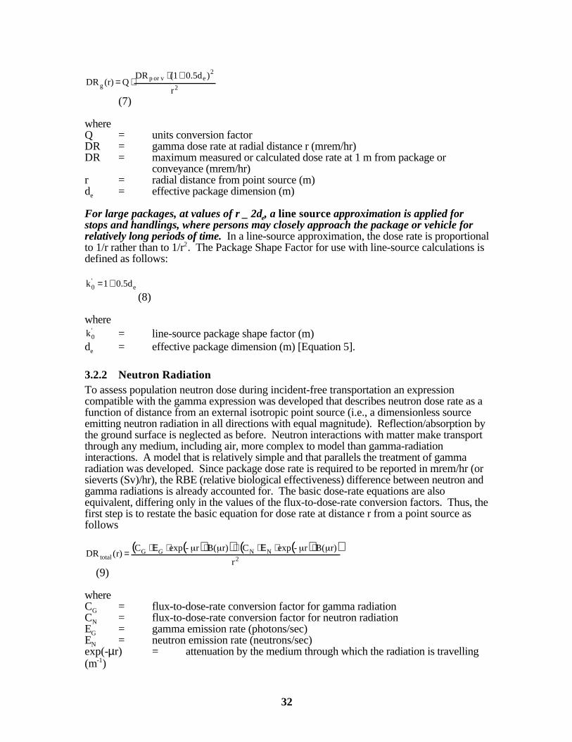
32

r

)0.5d(1 DRQ (r)DR

2

2eor v p

g

+⋅⋅=

(7)

whereQ = units conversion factorDR = gamma dose rate at radial distance r (mrem/hr)DR = maximum measured or calculated dose rate at 1 m from package or

conveyance (mrem/hr)r = radial distance from point source (m)de = effective package dimension (m)

For large packages, at values of r _ 2de, a line source approximation is applied forstops and handlings, where persons may closely approach the package or vehicle forrelatively long periods of time. In a line-source approximation, the dose rate is proportionalto 1/r rather than to 1/r2. The Package Shape Factor for use with line-source calculations isdefined as follows:

e'0 0.5d 1 k +=

(8)

where'0k = line-source package shape factor (m)

de = effective package dimension (m) [Equation 5].

3.2.2 Neutron RadiationTo assess population neutron dose during incident-free transportation an expressioncompatible with the gamma expression was developed that describes neutron dose rate as afunction of distance from an external isotropic point source (i.e., a dimensionless sourceemitting neutron radiation in all directions with equal magnitude). Reflection/absorption bythe ground surface is neglected as before. Neutron interactions with matter make transportthrough any medium, including air, more complex to model than gamma-radiationinteractions. A model that is relatively simple and that parallels the treatment of gammaradiation was developed. Since package dose rate is required to be reported in mrem/hr (orsieverts (Sv)/hr), the RBE (relative biological effectiveness) difference between neutron andgamma radiations is already accounted for. The basic dose-rate equations are alsoequivalent, differing only in the values of the flux-to-dose-rate conversion factors. Thus, thefirst step is to restate the basic equation for dose rate at distance r from a point source asfollows

( )( ) ( )( )

r

r)B(r-expC r)B(r-expC r)(DR

2NNG

total⋅⋅Ε⋅+⋅⋅Ε⋅= G

(9)

whereCG = flux-to-dose-rate conversion factor for gamma radiationCN = flux-to-dose-rate conversion factor for neutron radiationEG = gamma emission rate (photons/sec)EN = neutron emission rate (neutrons/sec)exp(-µr) = attenuation by the medium through which the radiation is travelling(m-1)

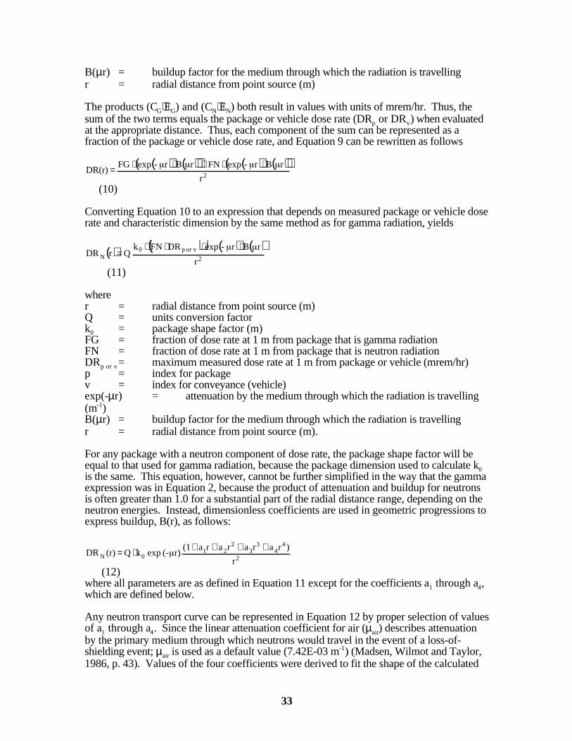
33

B(µr) = buildup factor for the medium through which the radiation is travellingr = radial distance from point source (m)

The products (CG⋅EG) and (CN⋅EN) both result in values with units of mrem/hr. Thus, thesum of the two terms equals the package or vehicle dose rate (DRp or DRv) when evaluatedat the appropriate distance. Thus, each component of the sum can be represented as afraction of the package or vehicle dose rate, and Equation 9 can be rewritten as follows

( ) ( )( ) ( ) ( )( )

r

rBr-expFN rBr-expFG DR(r)

2

⋅⋅+⋅⋅=

(10)

Converting Equation 10 to an expression that depends on measured package or vehicle doserate and characteristic dimension by the same method as for gamma radiation, yields

( ) ( ) ( ) ( )

r

rBr-expDRFNk Q rDR

2

or v p0N

⋅⋅⋅⋅=

(11)

wherer = radial distance from point source (m)Q = units conversion factork0 = package shape factor (m)FG = fraction of dose rate at 1 m from package that is gamma radiationFN = fraction of dose rate at 1 m from package that is neutron radiationDRp or v = maximum measured dose rate at 1 m from package or vehicle (mrem/hr)p = index for packagev = index for conveyance (vehicle)exp(-µr) = attenuation by the medium through which the radiation is travelling(m-1)B(µr) = buildup factor for the medium through which the radiation is travellingr = radial distance from point source (m).

For any package with a neutron component of dose rate, the package shape factor will beequal to that used for gamma radiation, because the package dimension used to calculate k0is the same. This equation, however, cannot be further simplified in the way that the gammaexpression was in Equation 2, because the product of attenuation and buildup for neutronsis often greater than 1.0 for a substantial part of the radial distance range, depending on theneutron energies. Instead, dimensionless coefficients are used in geometric progressions toexpress buildup, B(r), as follows:

r

)ra ra rar a (1r)(- exp kQ (r)DR

2

44

33

221

0N++++⋅=

(12)where all parameters are as defined in Equation 11 except for the coefficients a1 through a4,which are defined below.

Any neutron transport curve can be represented in Equation 12 by proper selection of valuesof a1 through a4. Since the linear attenuation coefficient for air (µair) describes attenuationby the primary medium through which neutrons would travel in the event of a loss-of-shielding event; µair is used as a default value (7.42E-03 m-1) (Madsen, Wilmot and Taylor,1986, p. 43). Values of the four coefficients were derived to fit the shape of the calculated

34

dose-vs.-distance curve in air to the shape of the selected neutron transport curve (Figure 3-1). These values are

a1 = 2.02E-02; (13)a2 = 6.17E-05;a3 = 3.17E-08;a4 = 0.

Significant levels of neutron radiation are seldom encountered in radioactive materialstransportation. The coefficient values provided here are intended to facilitate neutron doserate calculation in the main case for which such calculations might be appropriate – spentnuclear fuel transportation. The data are for fission neutrons; they were obtained withneutron cross section data from the ENDF/B-V cross section data library (Kinsey andMagurno, 1983) generated with the NJOY code (McFarlane et al., 1982). The source wasassigned an energy spectrum obtained from Oak Ridge National Laboratory calculations ofthe neutron flux at the surface of a lead-shielded spent fuel shipping cask. Neutrontransport calculations were performed with the ONEDANT code, which solves the one-dimensional (cylindrical) multigroup Bolttzmann transport equation by the discreteordinates method (O’Dell et al., 1982). The ENDF library, NJOY, and ONEDANT arediscussed and evaluated by Parks et al. (1988). A neutron transport curve through air at50% humidity was calculated because air molecules and water vapor significantly attenuateneutrons (but not gamma radiation). These default data are generally acceptable forapplications of RADTRAN 5 involving spent fuel. However, the user may carry out newneutron transport calculations and derive new coefficients that fit the resulting curve.

For a line source, the derivation is again similar to that for gamma radiation. It yields

r

)ra ra rar a (1r)(- exp k Q (r)DR

44

33

221'

0N++++⋅=

(14)

whereDRN(r)= neutron dose rate at distance r (mrem/hr)r = radial distance from source (m)Q = units conversion factor

'0k = line-source shape factor as defined above (m)

µ = linear attenuation coefficient (m-1); default is value for air, 7.42E-03 m-1

a1, a2 a3, a4 = dimensionless coefficients.

3.2.3 Summary of Final Expressions for Gamma and Neutron Radiation

Gamma and Neutron FractionsThe fractions of the dose rate that are gamma and neutron radiation are represented as fGand fN, respectively, throughout this technical manual, and the sum of the two must be unity(fG + fN = 1.0). Since the relative fractions of gamma and neutron change with distancefrom the package, values of fG and fN must be determined at the same 1-m distance fromthe package or vehicle surface as the dose-rate metrics DRp and DRv.

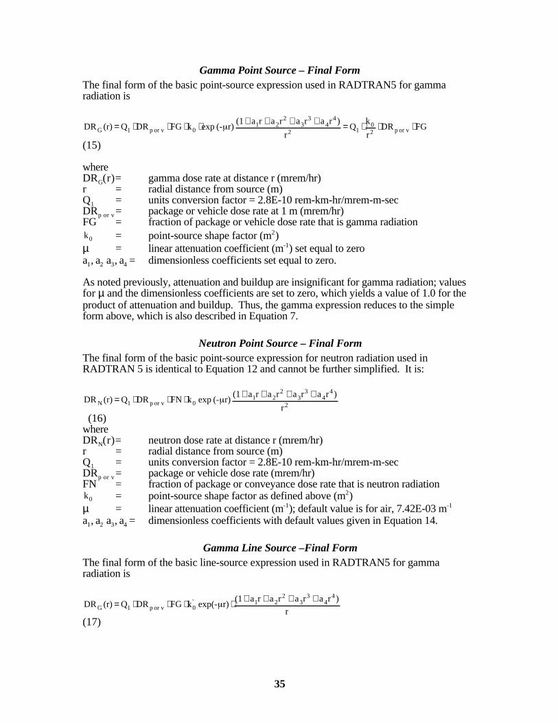
35

Gamma Point Source – Final FormThe final form of the basic point-source expression used in RADTRAN5 for gammaradiation is

FG DR r

kQ

r

)ra ra rar a (1r)(- exp kFGDRQ (r)DR or v p2

012

44

33

221

0or v p1G ⋅⋅⋅=++++⋅⋅⋅⋅=

(15)

whereDRG(r)= gamma dose rate at distance r (mrem/hr)r = radial distance from source (m)Q1 = units conversion factor = 2.8E-10 rem-km-hr/mrem-m-secDRp or v = package or vehicle dose rate at 1 m (mrem/hr)FG = fraction of package or vehicle dose rate that is gamma radiation

0k = point-source shape factor (m2)µ = linear attenuation coefficient (m-1) set equal to zeroa1, a2 a3, a4 = dimensionless coefficients set equal to zero.

As noted previously, attenuation and buildup are insignificant for gamma radiation; valuesfor µ and the dimensionless coefficients are set to zero, which yields a value of 1.0 for theproduct of attenuation and buildup. Thus, the gamma expression reduces to the simpleform above, which is also described in Equation 7.

Neutron Point Source – Final FormThe final form of the basic point-source expression for neutron radiation used inRADTRAN 5 is identical to Equation 12 and cannot be further simplified. It is:

r

)ra ra rar a (1r)(- exp k FNDRQ (r)DR

2

44

33

221

0or v p1N++++⋅⋅⋅=

(16)whereDRN(r)= neutron dose rate at distance r (mrem/hr)r = radial distance from source (m)Q1 = units conversion factor = 2.8E-10 rem-km-hr/mrem-m-secDRp or v = package or vehicle dose rate (mrem/hr)FN = fraction of package or conveyance dose rate that is neutron radiation

0k = point-source shape factor as defined above (m2)µ = linear attenuation coefficient (m-1); default value is for air, 7.42E-03 m-1

a1, a2 a3, a4 = dimensionless coefficients with default values given in Equation 14.

Gamma Line Source –Final FormThe final form of the basic line-source expression used in RADTRAN5 for gammaradiation is

r

)ra ra rar a (1 r)exp(- kFGDRQ (r)DR

44

33

221'

0or v p1G++++⋅⋅⋅⋅=

(17)

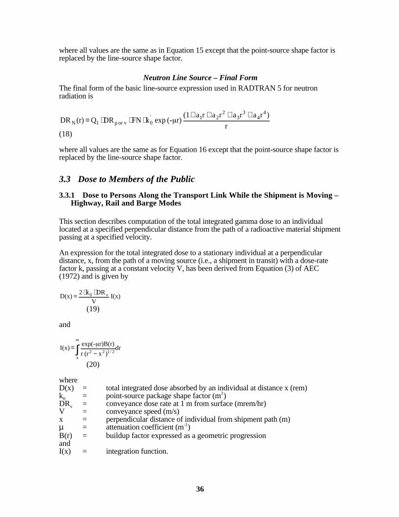
36

where all values are the same as in Equation 15 except that the point-source shape factor isreplaced by the line-source shape factor.

Neutron Line Source – Final FormThe final form of the basic line-source expression used in RADTRAN 5 for neutronradiation is

r

)ra ra rar a (1r)(- exp k FNDRQ (r)DR

44

33

221'

0or v p1N++++

⋅⋅⋅=

(18)

where all values are the same as for Equation 16 except that the point-source shape factor isreplaced by the line-source shape factor.

3.3 Dose to Members of the Public

3.3.1 Dose to Persons Along the Transport Link While the Shipment is Moving –Highway, Rail and Barge Modes

This section describes computation of the total integrated gamma dose to an individuallocated at a specified perpendicular distance from the path of a radioactive material shipmentpassing at a specified velocity.

An expression for the total integrated dose to a stationary individual at a perpendiculardistance, x, from the path of a moving source (i.e., a shipment in transit) with a dose-ratefactor k, passing at a constant velocity V, has been derived from Equation (3) of AEC(1972) and is given by

I(x)V

DRk2 D(x) v0 ⋅⋅=

(19)

and

dr)x(rr

r)B(r)exp(- I(x)

x2/122∫

∞

−=

(20)

whereD(x) = total integrated dose absorbed by an individual at distance x (rem)k0 = point-source package shape factor (m2)DRv = conveyance dose rate at 1 m from surface (mrem/hr)V = conveyance speed (m/s)x = perpendicular distance of individual from shipment path (m)µ = attenuation coefficient (m-1)B(r) = buildup factor expressed as a geometric progressionandI(x) = integration function.

37

To obtain the integrated population dose along a unit length of travel, Equation 19 ismultiplied by the population density and integrated over strips of width d on both sides ofthe transportation path:

∫⋅⋅=max

min

off D(x)dx PD Q 2 D

(21)where all variables are as defined in Equations 19 and 20 except for the following:Doff = integrated population dose per km of strip (person-rem)Q = units conversion factorPD = population density (persons/km2)min = minimum distance from population to shipment centerline (m)max = maximum distance perpendicular to shipment route over which exposure is

evaluated (m).

The value of max is usually set to 800 m (~ 0.5 mi.) because that is the value historicallyused in AEC (1972), and in earlier releases of RADTRAN. The value is not tied to anyanalytical results indicating that it is appropriate; indeed, dose rates generally fall belowdetectable levels well before a distance of 800 m from the source. However, retaining the800-m value is slightly conservative and does preserve parallelism and comparability witholder analyses. It is recommended that this value be used to establish a baseline forcomparison purposes even when the user selects another value of max for his or heranalysis.

By inserting the expression for D(x) [Equation 19] into Equation 21, the latter can berewritten as

∫⋅⋅⋅⋅⋅=max

min

v01off I(x)dx

V

PDDR k 4Q D

(22)where all variables are defined in Equations 20 and 21 and the units conversion factor, Q1, isevaluated as 2.8E-10 rem-km-hr/mrem-m-sec.

For incident-free transportation, the total population dose for persons along a transport linkis obtained in RADTRAN 5 by multiplying Equation 22 by the number of shipments of thetype being analyzed.

The integration of Equation 22 is performed by use of a Gaussian quadrature, GAUS8,which is a Sandia National Laboratories’ SLATEC math routine that integrates a realfunction of one variable over a finite interval (min to d, in this case).

The function integrated by GAUS8 is

dr) x(rr

r)r)B(exp(- (x)I

x2/122∫

∞

⋅=′

(23)

( ) 0 if ;eBESK1xa3

xa2 BESKO xa3 - a1 x

BSKIN s

x-sx

s

sssx

2ss

xss ≠⋅

⋅

⋅+⋅+⋅⋅+= ⋅⋅⋅

⋅

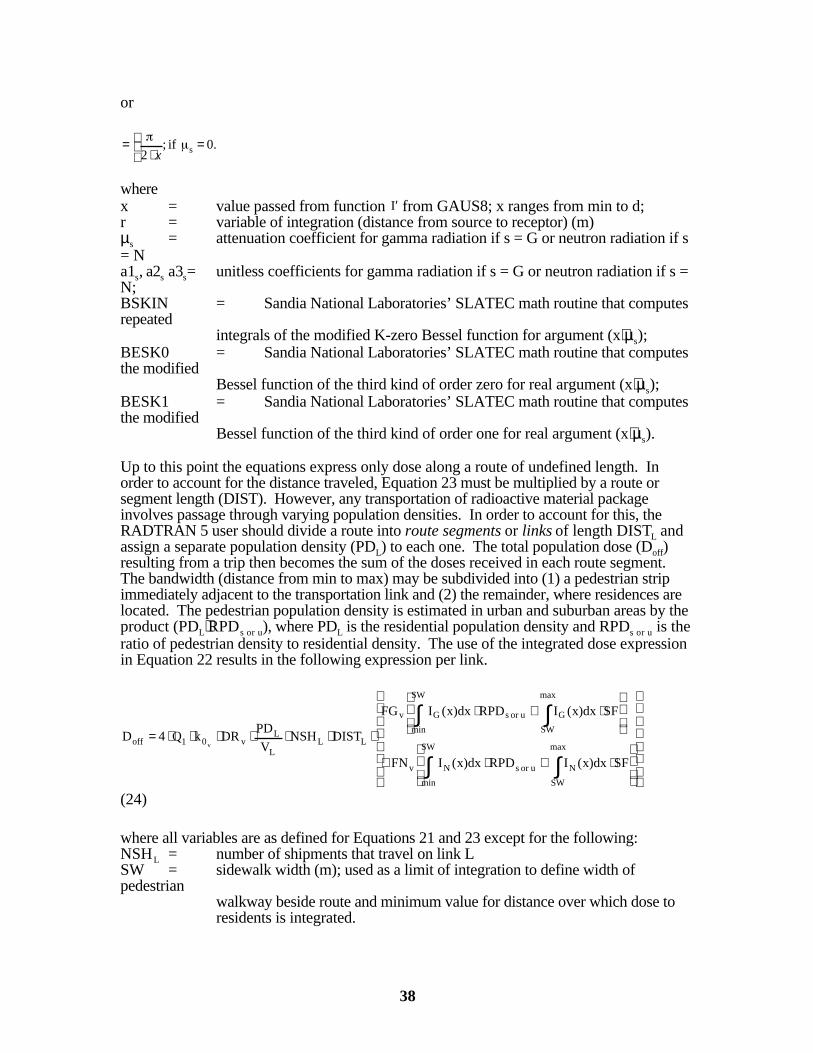
38

or

0. if ;2 s =

⋅=

x

wherex = value passed from function I′ from GAUS8; x ranges from min to d;r = variable of integration (distance from source to receptor) (m)µs = attenuation coefficient for gamma radiation if s = G or neutron radiation if s= Na1s, a2s a3s= unitless coefficients for gamma radiation if s = G or neutron radiation if s =N;BSKIN = Sandia National Laboratories’ SLATEC math routine that computesrepeated

integrals of the modified K-zero Bessel function for argument (x⋅µs);BESK0 = Sandia National Laboratories’ SLATEC math routine that computesthe modified

Bessel function of the third kind of order zero for real argument (x⋅µs);BESK1 = Sandia National Laboratories’ SLATEC math routine that computesthe modified

Bessel function of the third kind of order one for real argument (x⋅µs).

Up to this point the equations express only dose along a route of undefined length. Inorder to account for the distance traveled, Equation 23 must be multiplied by a route orsegment length (DIST). However, any transportation of radioactive material packageinvolves passage through varying population densities. In order to account for this, theRADTRAN 5 user should divide a route into route segments or links of length DISTL andassign a separate population density (PDL) to each one. The total population dose (Doff)resulting from a trip then becomes the sum of the doses received in each route segment. The bandwidth (distance from min to max) may be subdivided into (1) a pedestrian stripimmediately adjacent to the transportation link and (2) the remainder, where residences arelocated. The pedestrian population density is estimated in urban and suburban areas by theproduct (PDL⋅RPDs or u), where PDL is the residential population density and RPDs or u is theratio of pedestrian density to residential density. The use of the integrated dose expressionin Equation 22 results in the following expression per link.

⋅+⋅+

⋅+⋅

⋅⋅⋅⋅⋅⋅⋅=

∫ ∫

∫ ∫SW

min

max

SW

Nuor sNv

SW

min

max

SW

Guor sGv

LLL

Lv01off

SFx)dx(I RPDx)dx(IFN

SFx)dx(I RPDx)dx(IFG

DISTNSH V

PDDRkQ4 D

v

(24)

where all variables are as defined for Equations 21 and 23 except for the following:NSHL = number of shipments that travel on link LSW = sidewalk width (m); used as a limit of integration to define width ofpedestrian

walkway beside route and minimum value for distance over which dose toresidents is integrated.

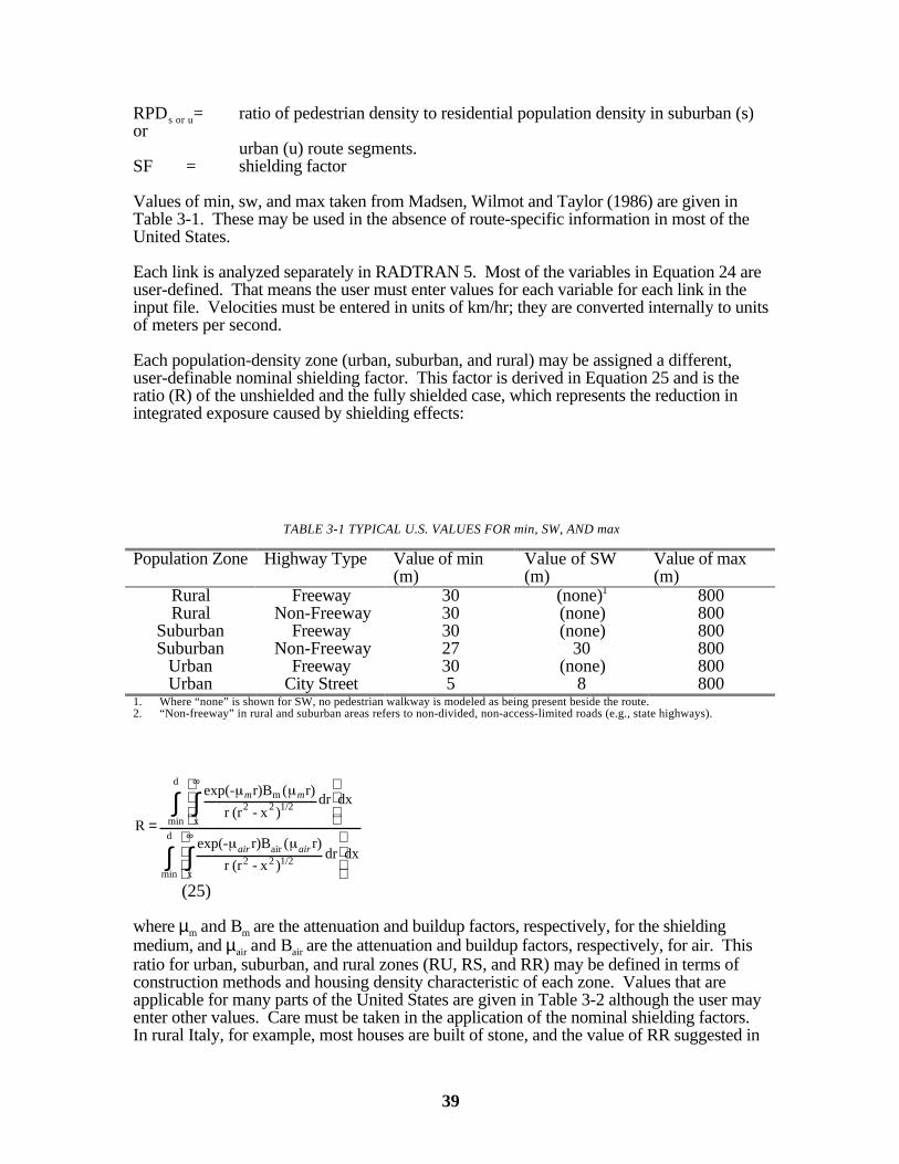
39

RPDs or u= ratio of pedestrian density to residential population density in suburban (s)or

urban (u) route segments.SF = shielding factor

Values of min, sw, and max taken from Madsen, Wilmot and Taylor (1986) are given inTable 3-1. These may be used in the absence of route-specific information in most of theUnited States.

Each link is analyzed separately in RADTRAN 5. Most of the variables in Equation 24 areuser-defined. That means the user must enter values for each variable for each link in theinput file. Velocities must be entered in units of km/hr; they are converted internally to unitsof meters per second.

Each population-density zone (urban, suburban, and rural) may be assigned a different,user-definable nominal shielding factor. This factor is derived in Equation 25 and is theratio (R) of the unshielded and the fully shielded case, which represents the reduction inintegrated exposure caused by shielding effects:

TABLE 3-1 TYPICAL U.S. VALUES FOR min, SW, AND max

Population Zone Highway Type Value of min(m)

Value of SW(m)

Value of max(m)

Rural Freeway 30 (none)1 800Rural Non-Freeway 30 (none) 800

Suburban Freeway 30 (none) 800Suburban Non-Freeway 27 30 800

Urban Freeway 30 (none) 800Urban City Street 5 8 800

1. Where “none” is shown for SW, no pedestrian walkway is modeled as being present beside the route.2. “Non-freeway” in rural and suburban areas refers to non-divided, non-access-limited roads (e.g., state highways).

∫ ∫

∫ ∫

=∞

∞

d

min x1/222

air

d

min x

1/222m

dxdr)x-(rr

r)(r)Bexp(-

dxdr)x-(rr

r)(r)Bexp(-

R

airair

mm

(25)

where µm and Bm are the attenuation and buildup factors, respectively, for the shieldingmedium, and µair and Bair are the attenuation and buildup factors, respectively, for air. Thisratio for urban, suburban, and rural zones (RU, RS, and RR) may be defined in terms ofconstruction methods and housing density characteristic of each zone. Values that areapplicable for many parts of the United States are given in Table 3-2 although the user mayenter other values. Care must be taken in the application of the nominal shielding factors. In rural Italy, for example, most houses are built of stone, and the value of RR suggested in

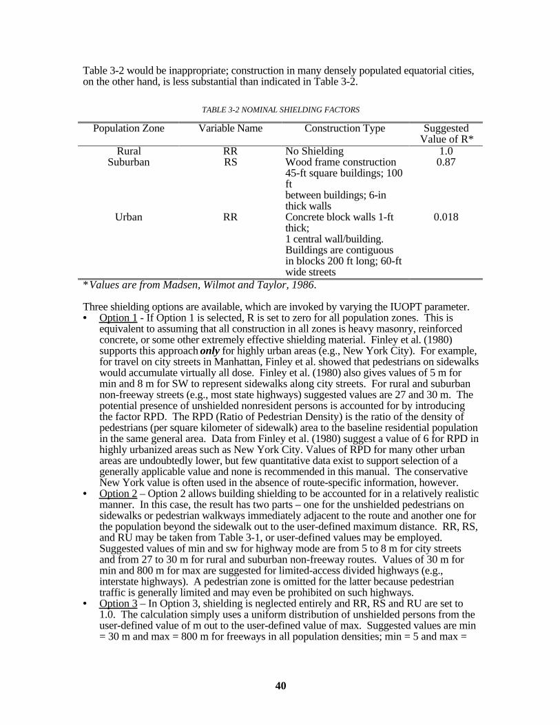
40

Table 3-2 would be inappropriate; construction in many densely populated equatorial cities,on the other hand, is less substantial than indicated in Table 3-2.

TABLE 3-2 NOMINAL SHIELDING FACTORS

Population Zone Variable Name Construction Type SuggestedValue of R*

Rural RR No Shielding 1.0Suburban RS Wood frame construction

45-ft square buildings; 100ftbetween buildings; 6-inthick walls

0.87

Urban RR Concrete block walls 1-ftthick;1 central wall/building. Buildings are contiguousin blocks 200 ft long; 60-ftwide streets

0.018

*Values are from Madsen, Wilmot and Taylor, 1986.

Three shielding options are available, which are invoked by varying the IUOPT parameter.• Option 1 - If Option 1 is selected, R is set to zero for all population zones. This is

equivalent to assuming that all construction in all zones is heavy masonry, reinforcedconcrete, or some other extremely effective shielding material. Finley et al. (1980)supports this approach only for highly urban areas (e.g., New York City). For example,for travel on city streets in Manhattan, Finley et al. showed that pedestrians on sidewalkswould accumulate virtually all dose. Finley et al. (1980) also gives values of 5 m formin and 8 m for SW to represent sidewalks along city streets. For rural and suburbannon-freeway streets (e.g., most state highways) suggested values are 27 and 30 m. Thepotential presence of unshielded nonresident persons is accounted for by introducingthe factor RPD. The RPD (Ratio of Pedestrian Density) is the ratio of the density ofpedestrians (per square kilometer of sidewalk) area to the baseline residential populationin the same general area. Data from Finley et al. (1980) suggest a value of 6 for RPD inhighly urbanized areas such as New York City. Values of RPD for many other urbanareas are undoubtedly lower, but few quantitative data exist to support selection of agenerally applicable value and none is recommended in this manual. The conservativeNew York value is often used in the absence of route-specific information, however.

• Option 2 – Option 2 allows building shielding to be accounted for in a relatively realisticmanner. In this case, the result has two parts – one for the unshielded pedestrians onsidewalks or pedestrian walkways immediately adjacent to the route and another one forthe population beyond the sidewalk out to the user-defined maximum distance. RR, RS,and RU may be taken from Table 3-1, or user-defined values may be employed. Suggested values of min and sw for highway mode are from 5 to 8 m for city streetsand from 27 to 30 m for rural and suburban non-freeway routes. Values of 30 m formin and 800 m for max are suggested for limited-access divided highways (e.g.,interstate highways). A pedestrian zone is omitted for the latter because pedestriantraffic is generally limited and may even be prohibited on such highways.

• Option 3 – In Option 3, shielding is neglected entirely and RR, RS and RU are set to1.0. The calculation simply uses a uniform distribution of unshielded persons from theuser-defined value of m out to the user-defined value of max. Suggested values are min= 30 m and max = 800 m for freeways in all population densities; min = 5 and max =

41

800 m for city streets; and min = 27 and max = 800 m for rural and suburban non-freeway links.

When a Highway-Route-Controlled Quantity (HRCQ) of radioactive material is shipped bytruck, the truck is required by USDOT regulations to travel on interstate highways or state-designated alternative routes. HRCQ and routing regulations for highway shipments aredefined and described in 49 CFR 171-177. In RADTRAN 5, interstate highways andsimilarly engineered highways are referred to as freeways. As already noted, freewaysare modeled as having no pedestrians. It is also recommended that the same averagevelocity be used for all freeway segments, regardless of population density.

“Virtual route segments” can be constructed to account for time spent in rush-hour trafficin urban or suburban areas. That is, route segments on which rush hour traffic is expectedcan be entered twice, once with a “normal” velocity and traffic density and once with arush-hour velocity and traffic density. The fractional representation of the rush-hoursegment (i.e., the fraction of time rush-hour conditions are encountered on the routesegment) is then accounted for by properly apportioning the total actual segment lengthbetween the two virtual segments. For example, if rush-hour traffic occurs for 4 hours perday on route segment x, then the fractional occurrence of rush-hour conditions is 4/24 or~0.17. If segment x is 40 km in length, then 40 x 0.17 = 6.8 km is the length of the virtualsegment to which the higher traffic density and lower average speed of rush-hour trafficshould be assigned, and the remainder (33.2 km) is the length of the “non-rush-hour”segment. In the absence of specific data, it is recommended that the traffic density bedoubled and the average velocity halved to represent rush-hour conditions. Route-specificdata are usually only available from state or local authorities (e.g., Brogan, Cashwell, andNeuhauser, 1989). State or local regulations such a time-of-day restrictions on RAMshipments through certain cities, may affect the choice of values for these parameters.

Rail, Ship and Barge ModesThe population doses received by persons along a rail transport link or waterway arecomputed in a manner identical to that used for highway modes. The limits of integration(values of min, SW, and max) vary by mode. For rail mode, value of 30 and 800 for minand max, respectively, are often used in the absence of route-specific information. The valueof sw is always zero for rail and water modes.

The 30-m value of min generally is a conservative representation of railroad right-of-waywidth, although larger and smaller values may be indicated by route-specific information. The 800-m value of max provides consistency and comparability with truck mode analysesand with earlier RADTRAN analyses. The user may select any value, but modal alternatives(e.g., truck mode versus rail mode) can only be meaningfully compared if the limits ofintegration are the same or if differences (e.g., differences between modes) have logicalexplanations and are accounted for in the analysis.

All open ocean travel and travel on certain inland waterways (e.g., the Great Lakes) takeplace in uninhabited areas. Portions of a route passing through these areas may be eitherremoved from the analysis or (preferably) assigned an off-link population density of zero. Passage on rivers, canals, congested port waters, etc. where a populated shoreline is within800 m of the vessel should be represented as segments with non-zero population densities. The value of min in such areas is dictated by the minimum distance from the navigablechannel to the shoreline. A suitable value for min in congested waterways in the absence oflocation-specific data is 200 m. The maximum limit of integration should remain the sameas that used for other modes if more than one mode is being analyzed; the standard valuefor all modes is 800 m.

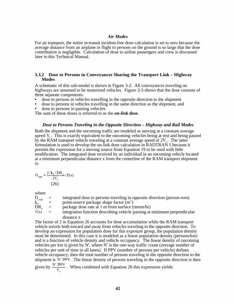
42

Air ModesFor air transport, the entire in-transit incident-free dose calculation is set to zero because theaverage distance from an airplane in flight to persons on the ground is so large that the dosecontribution is negligible. Calculation of dose to airline passengers and crew is discussedlater in this Technical Manual.

3.3.2 Dose to Persons in Conveyances Sharing the Transport Link – HighwayModes

A schematic of this sub-model is shown in Figure 3-2. All conveyances traveling onhighways are assumed to be motorized vehicles. Figure 3-3 shows that the dose consists ofthree separate components:• dose to persons in vehicles travelling in the opposite direction to the shipment• dose to persons in vehicles travelling in the same direction as the shipment, and• dose to persons in passing vehicles.The sum of these doses is referred to as the on-link dose.

Dose to Persons Traveling in the Opposite Direction – Highway and Rail ModesBoth the shipment and the oncoming traffic are modeled as moving at a constant averagespeed Vv. This is exactly equivalent to the oncoming vehicles being at rest and being passedby the RAM transport vehicle traveling at a constant average speed of 2Vv. The latterformulation is used to develop the on-link dose calculation in RADTRAN 5 because itpermits the expression for a moving source from Equation 19 to be used with littlemodification. The integrated dose received by an individual in an oncoming vehicle locatedat a minimum perpendicular distance x from the centerline of the RAM transport shipmentis:

(x)I2V

DRk2 D

v

v0opp ′⋅⋅⋅=

(26)

whereDopp = integrated dose to persons traveling in opposite direction (person-rem)k0 = point-source package shape factor (m2)DRv = package dose rate at 1 m from surface (mrem/hr)

(x)I′ = integration function describing vehicle passing at minimum perpendiculardistance x

The factor of 2 in Equation 26 accounts for dose accumulation while the RAM transportvehicle travels both toward and away from vehicles traveling in the opposite direction. Todevelop an expression for population dose for this exposure group, the population densitymust be determined. In this case it is modeled as a linear population density (persons/km)and is a function of vehicle density and vehicle occupancy. The linear density of oncomingvehicles per km is given by N′, where N′ is the one-way traffic count (average number ofvehicles per unit of time in all lanes). If PPV (number of persons per vehicle) definesvehicle occupancy, then the total number of persons traveling in the opposite direction to theshipment is PPVN ⋅′ . The linear density of persons traveling in the opposite direction is then

given by vV

PPVN ⋅′. When combined with Equation 26 this expression yields:

43

vLvv

v0opp NSHDISTPPV

VN

(x)IV

DRk2 D ⋅⋅⋅

′⋅′⋅⋅⋅= .

(27a)

This expression simplifies to:

vL2v

v0opp NSHDISTPPV(x)I

V

NDRk2D ⋅⋅⋅′⋅′⋅⋅⋅=

(27b)

whereDopp = integrated dose to persons in vehicles traveling in opposite direction (person-rem)k0 = point-source package shape factor (m2)DRv = dose rate at 1 m from surface of vehicle (mrem/hr)N′ = one-way traffic count (average number of vehicles per hour in all lanes)Vv = average velocity of all traffic (m/s)I′(x) = dose integration function from Equation 26PPV = vehicle occupancy (average number of persons per vehicle)DISTL = distance traveled on link LNSHv = number shipments of vehicle v.

The values of x in Table 3-3 are suggested values for common types of highway and raillinks. The values are user-definable, however, and may be changed as necessary toappropriately model the user’s problem. The primary distinction between freeways and theother two road classes is that interstates are built to engineering standards that prescribeminimum lane widths, etc., which translates into a somewhat larger value of x.

Table 3-3 Minimum Perpendicular Lane-Separation Distances by Link Type

Type of Link Value of x (meters)Freeway (Interstate Highway) 15

Two-Lane Highway (e.g. State Hwy.) 3City Street 3

Rail (double track) 3

By reference to Equation 24, a final expression for Dopp may be given as:

( ) ( )[ ])x(IFN)x(IFGV

NPPVDISTNSHDRkQ D NGv2

LLLv02 ′⋅+′⋅⋅′⋅⋅⋅⋅⋅⋅=

(28)where all variables are as given in Equations (24) and (27) excepting the following:Q2 = units conversion factor = 7.7E-08 rem-hr2-m/mrem-sec2-km.I′G = dose integration function for gamma radiationI′N = dose integration function for neutron radiation.

44

Figure 3-2 Illustration of Highway Traffic for Calculation of On-Link Dose

Dose to Persons Traveling in the Same Direction – Highway Mode Only

Trucks carrying radioactive material are modeled as moving at the same average velocity asthe rest of the traffic. Thus, vehicles traveling in the same direction as the RAM shipmentcan be considered to be stationary with respect to the RAM vehicle and can be modeled as alinear continuum of vehicles beginning at some minimum distance beyond the RAMvehicle. The dose received by a person located at distance r from the shipment vehicle iscomputed by multiplying the dose rate from Equation 4 by the duration of exposure t (hr):

2v0

sdirr

tDRkD

⋅⋅=

(29)

where all values are the same as in Equation 4 except for t, which is exposure time (hr).

For a given mode and link, the total exposure time t is given by the quotient of total distanceand average velocity (V); total distance traveled is, in turn, the product of distance pershipment and number of shipments. Thus,

L

LL

V

NSHDIST t

⋅=

(30)

45

People are modeled as being distributed uniformly among the vehicles with a linearpopulation density given by (N′⋅PPV)/V. The dose to persons traveling in the samedirection as the shipment is, therefore, the product of the dose expression in Equation 29and the linear population density (Equation 30) integrated from some minimum distance(min-sdir) to infinity:

∫∞

⋅

⋅⋅

⋅′⋅⋅⋅=

sdir-min2v0sdir dr

r

r)r)B((- exp

V

NSHDIST

V

PPVNDRk2 D

(31)

where all values are the same as in Equations 29 and 30 except for the integral, which is thebasic dose integration function for the RAM shipment. The factor of 2 in Equation 31accounts for the fact that traffic is modeled as extended in two directions – both in front ofand behind the RAM shipment.

In addition to persons in vehicles both in front of and behind the RAM shipment, the caseof a passing vehicle is considered. The full value of the traffic count N′ is used in Equation31 to estimate dose to the former. This in effect counts all vehicles in all lanes but treatsthem as though they were all in the same lane as the RAM shipment. The minimumexposure distance (min-sdir) depends on the average velocity, V, and therefore on the on-link population density, because the closest vehicle is modeled a being within 2 sec of travelof the RAM shipment. Thus, min-sdir (in meters) is given by the absolute value of 2V,where V is in units of m/sec. The average velocity is a user-defined input value and isentered in units of km/hr. RADTRAN 5 internally converts this value to m/sec. Theintegration in Equation 31 is performed with a Gaussian quadrature. Let the integral fromEquation 31 be represented as Yv. Then:

( ) ( ) ( ) ( )[ ]NV,GV,

2V2

Nr-

2V2

Gr-

v PFNPFGdr r

rBeFNdr

r

rBeFG Y

NG

⋅+⋅=

⋅⋅+

⋅⋅= ∫∫∞∞

(32)

whereFG = fraction of DRv that is gamma radiationFN = fraction of DRv that is neutron radiationV = average velocity (m/s)µG, µN = attenuation coefficients for gamma and neutron radiation (m-1)PV,G or PV,N = value of integral passed from Equation 31.

The value of P is determined as follows:

+

⋅++

⋅+++⋅+⋅=≠ ⋅⋅

SS

S23

S

S2

S

S3

S

S2

S

S

S

SV2-2V)(SSv,S

a4V2

a42a32V

a42a3a2

V2

1e E1) - (a1 P 0; If S

or

2V

1 P 0; If Sv,S ==

(33)

whereS = subscript for gamma (S = G) or neutron (S = N) radiation

46

E1 = Sandia National Laboratories SLATEC math routine that computes thesingle-

precision exponential integral for positive, single-precision argument (µS⋅2V)

V = average velocity (m/sec)2V = absolute value of minimum separation between vehicles (m)µS = attenuation coefficient for gamma (S = G) or neutron (S = N) radiation (m-1)a1S,...a4S= coefficients for gamma (S = G) or neutron (S =N) radiation.

By use of the same traffic characteristics as in the calculation of dose to persons traveling inthe opposite direction and by incorporation of the results of this integration, the followingexpression is obtained for the dose received by persons traveling in the same direction asthe shipment:

( )21vLL2L

Lv02sdir F FNSHDISTPPV

V

NDRkQ D +⋅⋅⋅⋅′⋅⋅⋅=

(34)

whereQ2 = units conversion factor = 7.7E-08 rem-hr2-m/mrem-sec2-kmk0 = point-source shape factor (m2)DR = dose rate at 1 m for the surface of vehicle v (mrem/hr)N′L = one-way traffic count on link L (vehicles/hr)VL = average velocity on link L (m/sec)PPVL = vehicle occupancy on link L (persons/vehicle)DISTL = distance traveled on link L (km)NSHv = number of shipments of vehicle vF1, F2 = traffic factors defined below.

F1 accounts for all vehicles except those passing the RAM shipment, while F2 accounts forpersons in vehicles in the passing lane immediately adjacent to the RAM shipment.

F1 = 2YvVL (35a)

and

Lv2 VYx

1 F ⋅=

(35b)

wherex = minimum perpendicular distance to adjacent vehicle.

A dose is computed for each shipment and route segment (link) with Equation 34, and theresults are summed over all shipments and links to obtain a total dose to persons travelingalong the route in the same direction as the RAM shipment(s) being analyzed.

3.3.3 Dose to Airline Passengers – Passenger-Air Mode

47

The following equations are used to formulate dose to air passengers under normalconditions of transport. The formulation of the dose to air passengers is based in part onempirical data developed by Barker et al. (1974). In Barker’s analysis, an empirical value of3E-05 rem/hr/TI for air passengers was derived (where Barker’s variable TI is the same asDRp). Thus, the integrated dose formulation becomes

L

Lpassvp3airpass V

DISTNSHNDRkQ D ⋅⋅⋅⋅⋅=

(36)

whereDairpass = integrated population dose to air passengers (person-rem)Q3 = units conversion factor = 0.28 m-hr/km-seckp = empirical dose-rate conversion factor (3E-05 rem/hr/TI)DRv = dose rate at 1 m from surface of shipment on aircraft v (mrem/hr)Npass = number of air passengers on boardNSHv = number of shipments by aircraft vDISTL = distance traveled on link L (km)VL = average velocity on link L (m/sec).

3.4 Dose to Population at Shipment Stops – All Modes

If a transport conveyance stops for a crew change, passenger transfer, crew meals, refueling,storage, inspection, or any other cause, then persons at or near the stop point can be exposedto radiation from the shipment. RADTRAN 5 presents the user with a choice of twodistinct ways to represent persons at stops.

3.4.1 Option 1 – Average-Distance MethodThe first option is a simple model based on the number of nearby persons and a specifiedaverage distance. This method has been used to model truck stops (Madsen and Wilmot,1983) and intermodal transfers at maritime ports (Neuhauser and Weiner, 1992). Theequation for integrated population dose (D) for Option 1 is:

( ) ( )[ ]( )

( )

source liner

k

sourcepoint r

k

TRFNTRFGSFPTNSH DR Q D

st

o

2st

o

rN,vrG,vstststvv4v

v

stst

′⋅⋅+⋅⋅⋅⋅⋅⋅⋅=

or

(37)whereQ4 = units conversion factor = 1.0E+03 rem/mrem

v0k = point-source conveyance shape factor (m2)

v0k′ = line-source conveyance shape factor (m)DRv = conveyance dose rate at 1 m from surface (mrem/hr)NSHv = number of shipmentsTst = average stop time (hr)Pst = average number of exposed personsSFst = shielding factor for stop population

48

FGv = fraction of vehicle dose rate from gamma radiation at origin pointFNv = fraction of neutron dose rate from neutron radiation at origin pointTRG = term for gamma radiation source strength at distance rTRN = term for neutron radiation source strength at distance rrst = average radial source-to-receptor distance at stops (m).

Ostmeyer (1986a) derived a shielding factor of 0.1 for rail stops, which reflects gammaattenuation by other railcars and structures in classification yards. The source-strengthterms, TRG and TRN, used in Equation 37 were derived from Equations 17 and 18. Theirexpanded form can be written as follows:

( ) [ ][ ]43G

2G

r-G ra4 ra3ra2 r a1 1e TR ⋅+⋅+⋅+⋅+⋅= ⋅

GGG

(38a)

and

( ) [ ][ ]4N

3N

2NN

r-N ra4 ra3ra2 r a1 1e TR ⋅+⋅+⋅+⋅+⋅= ⋅N

(38b)

whereµ = attenuation coefficient for gamma (µG) or neutron (µN) radiation (m-1)r = radial distance from source (m)a1...a4 = coefficients for gamma or neutron radiation.

Option 1 may be used for all transportation modes, although Option 2 is preferred for rail-mode calculations (see below).

3.4.2 Option 2. Annular-Area Method

In this option, dose is calculated for a population density within an annular area. Thisalternative is preferred for railyards and similar situations (Ostmeyer, 1986a). Many railstops occur in railyards, and the vast majority of total train stop time occurs in railyards. InOption 2, the population in and near a railyard is modeled as a uniformly distributedpopulation around the rail shipment; dose is then integrated over this population. Doses torailyard personnel who are involved in the inspection and maintenance of railcars (i.e.,persons who are exposed at short distances from the shipment) are dealt with separately. Data developed by Griego, Smith and Neuhauser (1996) also allow Option 2 to be appliedto truck stops.

The first step in calculation of stop dose with Option 2 involves integration over an annulararea from radial distance xmin to some radial distance xmax while accounting for buildup andattenuation. These values will be used to modify the initial source strength (DRv). This term(IRS) is evaluated for gamma (S = G) and neutron (S = N) radiation as follows:

( )( )

( ) ( )xE1 e 6x63xx

a

22xxa 1x

a

a

xIR Sx-

432S

23

4

3S

2SS

3SS

2

S

1

SS

S

S

SS

⋅+

+++

+

+++++

= ⋅

SSS

(39)

49

whereµS = attenuation coefficients for gamma (S = G) or neutron (S = N) radiation inair (m-1)a1...a4 = curve-fitting coefficients (see Equations 17 and 18) for gamma (S = G) orneutron (S = N)x = radial distance from source to receptor (m)E1 = SLATEC routine that computes the single precision exponential integral

for positive, single precision argument (µS⋅x).

The second step is to subtract the evaluation of the integral at xmax from the evaluation of theintegral at xmin, where max and min are the maximum and minimum radii, respectively, of theannular area. This is accomplished as follows:

{ ( ) ( )[ ] ( ) ( )minlnmaxln min

maxln 0; or maxIRminIR 0; C SSSSS −=

=−≠=

(40)

whereCS = source-strength modifier over defined intervalµS = attenuation coefficient for gamma (µG) or neutron (µN) radiation (m-1)IRS = value from Equation 39min = xmin = minimum value of radial distance from source (inner radius ofannulus) (m)max = xmax = maximum value of radial distance from source (outer radius ofannulus) (m)

When the values CG and Cn are used in place of TRG and TRN from Equation 38, the Option2 stop-dose equation results, as is shown:

( ) ( )[ ] CFNCFG SF NSH T PD DR k Q2 D NGstvststv04stopv

+⋅⋅⋅⋅⋅⋅⋅⋅=

(41)

whereQ4 = units conversion factor = 1.0E-03 rem/mrem

v0k = point-source shape factor for vehicle v (m2)DRv = vehicle dose rate at 1 m from surface (mrem/hr)PDst = population density of annular area at stop (persons/km2)Tst = duration of stop (hr)NSHv = number of shipments by vehicle vSFst = shielding factor at stopFG = fraction of DRv that is gamma radiationFN = fraction of DRv that is neutron radiation.

Evaluation for a line source is identical to that shown in Equation 41 except that the line-source shape factor

v0k′ is substituted for the point-source shape factor.

3.4.3 Use of Stop Model to Estimate Storage-Related DoseUnlike its predecessors, RADTRAN 5 does not contain a separate mathematical model forstorage dose. A period of storage that may occur during the course of transportation is infact simply a prolonged stop. Either of the two stop-dose models described above (Sections3.4.1 and 3.4.2) may be used to estimate dose to storage warehouse personnel. With each

50

option, a shielding factor may be entered to account for shielding by other packages instorage in the same warehouse, and by other barriers, if any. No value can be recommendedfor the shielding factor. The user may estimate a value from location and shipment specificdata, if available; otherwise, the shielding factor may be set to 1.0 (no shielding).

3.5 Dose to Workers

3.5.1 Dose to Crew Members – Highway and Air ModesThis section considers only crew members on conveyances while the shipment is en route. Other transportation workers, such as handlers and inspectors, are considered in thefollowing sections. Since crewmembers remain stationary with respect to the package(s) ona vehicle during all or most of a trip, the dose calculation is similar to that for a stop. However, the position of crewmembers with respect to a package may dictate that a differentcharacteristic package dimension should be used. This is the case, for example, with trucktransportation of spent fuel; the package dimension most appropriate for calculation of crewdose is cask diameter rather than cask length.

The calculation of dose to crewmembers is analogous to that given in Section 3.4. Thesurface of the package or “vehicle” (e.g., end of semi-trailer) nearest to the crew area ismodeled as a point source with the following situation-specific attributes:• k0,end, calculated for characteristic dimension, de,end; • source-to-worker distance, rend.• shielding factor to account for shielded crew compartments.

Thus,

( ) ( )[ ]rN,vrG,vvLL

crewvv2end

end0,1crew TRFNTRFGCSFDIST

V

1NNSHDR

r

k Q D ⋅+⋅⋅⋅⋅⋅⋅⋅⋅⋅=

(42)whereDcrew = integrated dose to crew (person-rem)Q1 = units conversion factor (2.8E+10 rem-m-hr/mrem-km-sec)ko,end = “crew-view” point-source package shape factor for de, end, where de, end is the

characteristic dimension of the package surface nearest to the crew (m2)rend source-to-worker distance (m)DRv = vehicle dose rate at 1 m from surface (mrem/hr)NSH = number of shipmentsNcrew = number of crew membersVL = average velocity on link LDISTL = distance traveled on link LCSFv = crew shielding factor for vehicle vFGv = fraction of vehicle dose rate from gamma radiationFNv = fraction of vehicle dose rate from neutron radiationTRG,r = dose-distance relationship factor for gamma radiationTRN,r = dose-distance relationship factor for neutron radiation.

51

3.5.2 Dose to Workers – Rail Mode

In-Transit Doses that are not Explicitly ModeledRADTRAN 5 does not contain an explicit model for calculating dose to the operating crewof a train while in transit because of:1. The massive amount of shielding provided by engines,2. The shielding provided by the intervening buffer cars required by regulation, and3. The relatively large separation distances between a RAM-carrying railcar and the engine

crew.Analysts with a need to examine such doses may treat the crew as persons at a stop with thestop time set equal to the time in transit of the train and the distance set equal to the crew-to-railcar distance. Accounting for shielding, perhaps by hand calculation, is necessary,however, to generate a realistic dose estimate.

Doses to Workers in Rail YardsDoses are estimated for rail workers who are in close proximity to the casks duringinspection and classification of cars at rail yards (Ostmeyer, 1986a). Two cases arediscussed: general freight and dedicated train shipment of radioactive material.

Because this dose is estimated for an inspector, classifier or other worker who is close to therailcars, which are large with respect to the worker, line-source geometry applies. The dosereceived by a worker for each classification and/or inspection operation is given by

( ) ( )[ ]NvGvvv01 workerrail RFNRFGNSHDRk Q D ⋅+⋅⋅⋅⋅′⋅= (43)

whereDrailworker = rail worker dose (person-rem)Q1 = units conversion factor (2.8E+10 rem-m-hr/mrem-km-sec)

ok′ = line-source rail-car shape factor (m)DRv = dose rate at 1 m of rail car v (mrem/hr)NSHv = number of shipments by rail car vFG = fraction of rail-car dose rate from gamma radiationFN = fraction of rail-car dose rate from neutron radiationand

⋅+⋅+⋅+⋅⋅+⋅+⋅+⋅+⋅+⋅+⋅

= train dedicated if :bTRbTRbTRbTR

freight general if ;bTRbTRbTRbTRbTRbTR bTR R

11S,9.010S,8.09S,4.08S,3.0

7S,20.06S,9.05S,8.04S,7.03S,5.02S,4.01S,3.0S

where S is G (gamma) or N (neutron) and bn is an exposure factor (person-hr/m).

Values of bn are calculated from data given in Wooden (1986) (see Appendix B). The totaldose to workers during classification and inspection in rail yards (DCL) is given by

NCL D D workerrailCL ⋅= (44)

whereDrail worker= dose to rail worker per classification or inspection from Equation 43NCL = number of classifications or inspections per trip

52

The total number of classifications per trip (NCL) is determined as follows

( )L

links all

DISTDDC DIC NCL ⋅+= ∑

(45)

whereDIC = the number of distance-independent classifications per tripDDC = the number of distance-dependent classifications per kmDISTL = length of link (km)

DIC represents the inspections that occur regardless of total trip distance. That number isdetermined by railroad company practices and is usually equal to two – one at the beginningand one at the end of each trip (Wooden, 1986). Federal regulations (49 CFR) require thatrailcars carrying hazardous material, including radioactive material, be inspected atinterchanges. The number of interchanges per link is dependent on the length of the link(DISTL). The recommended value for DIC is 2; the recommended value for DDC isderived from Ostmeyer (1986) and is 0.0018 inspections per km.

3.5.3 Dose to Cargo Inspectors on Waterborne Vessels

As in the rail case, crewmembers aboard waterborne vessels are shielded by ship structuresand generally are separated from the source locations (usually ship holds) by largedistances. Therefore, no general crew dose is calculated in RADTRAN 5 for these modesof transport. However, periodic inspections of the packages are required. Since radioactivematerial must be physically separated from other types of cargo, the vehicle subscript (v)applies to a cargo hold of a ship or a deck stowage area of a barge rather than to the entirevessel. The inspector is modeled as being an average of 2 m away from the package orpackage array during the inspection, which requires the package or package array to betreated as a line source for all but very small packages. Since the latter are seldom, if ever,shipped by waterborne modes, the following relationship applies to all cases.

day-m

min-person 0.5

m 2

1min 1

day

person 1 =⋅⋅

(46)

The integrated dose to cargo inspectors aboard waterborne vessels is given on a per-cargo-hold basis by

( ) ( )[ ]NvGvvV

NSHDISTDRend0,5inspector cargo TRFNTRFGCSFkQ 0.5 D

L

vLv ⋅+⋅⋅⋅⋅′⋅⋅= ⋅⋅

(47)

where0.5 = value from Equation 46 (person-min/m-day)Q5 = units conversion factor = 2.0E-07 m-hr-day/km-sec-min

end 0,k′ = “crew-view” line-source shape factor (m)DRv = cargo-hold dose rate at 1 m from surface (mrem/hr)DISTL = distance traveled on link L (km)NSHv = number of shipments by conveyance v (cargo-hold)VL = average velocity on link L (m/sec)

53

CSFv = crew shielding factor for cargo hold vFGv = fraction of cargo-hold dose rate from gamma radiationFNv = fraction of cargo-hold dose rate from neutron radiationTRG,2 = dose-distance relationship factor at 2 m for gamma radiationTRN,2 = dose-distance relationship factor at 2 m for neutron radiation.

The choice of shape factor deserves discussion. Equation 47 uses end 0,k′ , a line-sourcepackage shape factor, which is calculated with a characteristic package dimensionappropriate to the “view” of a worker. The latter can vary from being equal to that forpersons farther from the shipment (for a cubical or spherical package) to being less thanone-half of the dimension used to develop a k0 for the general public (for a long cylindricalpackage such as a spent-fuel cask). The actual view(s) presented to a ship-hold inspectordepends on package shape, ship size, and stowage practices. The user is cautioned tocarefully select an “inspector-view” package dimension when entering data for aRADTRAN analysis of transportation by water mode. In most cases the crew-shieldingfactor (CSF) will be 1.0, but the user has the option of altering the parameter in cases whereinspectors are partially shielded by intervening structures (e.g., a cask inside a steeltransportainer).

3.5.4 Dose to Flight Attendants – Passenger Air Mode

The following equations are used to formulate dose to flight attendants under normalconditions of transport. The flight-attendant dose should be added to the crew dose (pilot,co-pilot and/or navigator) to give total occupational dose for passenger-air mode. Theformulation of the dose to flight attendants is based in part on empirical data developed byBarker et al. (1974). In Barker’s analysis, an empirical value of 3E-05 rem/hr/TI for flightattendants was derived (where Barker’s term, TI, is synonymous with DRv as used here). Thus, the integrated dose formulation becomes

L

Lvflattvp3air V

DISTNSHNDRkQ D ⋅⋅⋅⋅⋅=

(48)

whereDair = integrated population dose to flight attendants (person-rem)Q3 = units conversion factor = 0.28 m-hr/km-seckp = empirical dose-rate conversion factor (3E-05 rem/hr/DRp)DRv = dose rate at 1 m from shipment surface in cargo hold of aircraft (mrem/hr)Nflatt = number flight attendants on boardNSHv = number of shipments by aircraft vDISTL = distance traveled on link L (km)VL = average velocity on link L (m/sec)

3.5.5 Dose to Handlers

Packages are handled during transportation primarily at intermodal transfers and duringtrips involving multiple deliveries (e.g., a van carrying many small packages ofradiopharmaceuticals from a central distribution point to several hospitals in a city). Handling is defined to include all operations concerned with the following:• transfer from one mode to another;• transfer from the originator’s shipping dock or other facility to the first conveyance;

54

• transfer from the final conveyance to the destination shipping dock or other facility.

To evaluate dose to package handlers, packages are divided into two groups according totheir size and the equipment necessary to move them. The two basic types are:• small packages that are readily manipulated by a single person;• all other packages (intermediate to large sizes).

To discern which type should be indicated, the input value for package size, dp, is comparedwith a package-threshold value (SMALLPKG). If SMALLPKG is not exceeded, then thepackage is of the first type; if SMALLPKG is exceeded, then the package is of the secondtype. The recommended value for SMALLPKG is 0.5 m. Although it is unlikely that thisvalue will need to be altered, the user may do so.

Small Packages (dp _ SMALLPKG)

Shapiro (1977) concludes that the average dose received by workers handling smallpackages of radioactive material is 2.5E-04 rem/handling/TI (where Shapiro’s TI is thesame as DRp). The absorbed dose per handling to handlers of small packages is given by:

( ) ( )[ ]HdN,pdG,pvpHHsmall TRFNTRFGNSHPPSDRk D

H⋅+⋅⋅⋅⋅⋅=

(49)

whereDHsmall = integrated dose to handlers of small packages (person-rem)kH = handling-to-dose conversion factor for small packages = 2.5E-04

rem/handling/DRpDRp = package dose rate at 1 m from surface (mrem/hr)PPS = number of packages per shipmentNSHv = number of shipments by vehicle vFGv = fraction of cargo-hold dose rate from gamma radiationFNv = fraction of cargo-hold dose rate from neutron radiationTRG,d = dose-distance relationship factor at distance d for gamma radiationTRN,d = dose-distance relationship factor at distance d for neutron radiationdH = average package-to-handler distance (m).

Point-Source for Intermediate- and Large-Sized Packages (dp SMALLPKG)

This calculation is used when the package-to-handler distance is greater than 2 times thecharacteristic package dimension. Handling of intermediate-sized packages such as 55-galdrums or large crates may require heavy equipment such as fork lifts or power assists andseveral people working simultaneously. The package is modeled as being stationary withrespect to the handler(s). This situation is similar to the stop-dose calculation in that acertain number of persons are modeled as being at a fixed distance from the package for acertain period of time:

( ) ( )[ ]HH dN,vdG,vvH2

H

p04H TRFNTRFGNSHPPHT

d

PPSDRkQ D ⋅+⋅⋅⋅⋅⋅

⋅⋅⋅=

(50)

whereDH = integrated dose to handlers of medium and large packages (person-rem)

55

Q4 = units conversion factor = 1.0E-03 rem/mremk0 = point-source shape factor (m2)DRp = package dose rate at 1 m from package surface (mrem/hr)TH = average exposure time of handlers (hr)PPS - number of packages per shipmentdH = average package-to-handler distance (m)NSHv = number of shipments of vehicle vFGv = fraction of cargo-hold dose rate from gamma radiationFNv = fraction of cargo-hold dose rate from neutron radiationTRG,dH = dose-distance relationship factor at distance dH for gamma radiationTRN,dH = dose-distance relationship factor at distance dH for neutron radiation.

Line-Source Calculation for Intermediate- and Large-Sized Packages (dp SMALLPKG)

This calculation is used when the package-to-handler distance is less than twice thecharacteristic package dimension. When radiological inspection, the attachment/detachmentof rigging equipment, etc. require inspectors and/or handlers to closely approach thepackage, a point-source geometry is inappropriate. Line-source geometry is used instead(Weiner and Neuhauser, 1992). Thus,

( ) ( )[ ]HH

d N,vdG,vvHH

vp04Hline TRFNTRFGNSHPPHT

d

PPSDRkQ D ⋅+⋅⋅⋅⋅⋅

⋅⋅′⋅=

(51)

where all parameters are the same as in Equation 50 except that k0 is replaced by 0k′ and the

denominator is Hd rather than 2Hd .

56

4 ATMOSPHERIC DISPERSION

An accident involving a shipment of radioactive material does not pose a hazard beyond theimmediate vicinity of the accident unless material is released from the package(s) in adispersible form. Atmospheric dispersion of aerosols and gases (dispersible forms) ismodeled in RADTRAN 5. Principles of atmospheric dispersion are summarized in thischapter. Consequences of dispersal are evaluated in Chapter 5.

4.1 Basic Principles of Atmospheric Dispersion

Materials released into the air in particulate or gaseous form at the scene of an accident aredispersed as they are transported downwind, and diffuse vertically and laterally (crosswind)according to the degree of turbulence in the atmosphere. Although other representations arepossible, most commonly used mathematical representations of atmospheric dispersion arebased on a Gaussian plume model, developed by Pasquill (1961), in which gases or particlesreleased into the atmosphere and dispersed exhibit ideal gas behavior. The principles onwhich the model is based are:

• The predominant force in plume transport is the wind; i.e., gases, aerosols, and particlesdispersed in the air move predominantly downwind.

• The greatest concentration of material in a plume is along the plume centerline.

• Aerosols, gases, and other materials in a plume diffuse spontaneously from regions ofhigher concentration to regions of lower concentration.

In Gaussian models for a “puff” release (i.e., for an idealized instantaneous, perfectlyspherical release), the concentration of the material in the puff has a normal distributionalong the two axes perpendicular to wind direction (Figure 4-1). With few exceptions,source clouds for releases associated with transportation accidents should be modeled aspuff releases. Unless a fire or other heat source lofts released material more than 10 meters,releases from transportation accidents occur at ground level and should be modeledaccordingly. Source clouds for severe fires that might loft material above an accident siteare sometimes modeled as cylinders (e.g., as done in the DIFOUT dispersion code; Lunaand Church, 1969). The Gaussian models for continuous releases such as those fromsmokestacks (elevated releases) or pipeline leaks (ground-level releases) are inappropriatefor use in transportation risk analysis.

Persons in the path of such an aerosol plume inhale material as the plume passes, andinhaled particles are deposited in their lungs in proportion to the time-integratedconcentration [denoted by Χ (Greek letter chi) and having units of Ci-sec/m3 or Sv-sec/m3]of the aerosol. For radioactive materials, the value of Χ at any point downwind of therelease location is directly proportional to the total activity of the released aerosol species[Q, with units of activity; curies (Ci) in RADTRAN 5] and is inversely proportional to thewind speed (u with units of m/sec). One way of describing the behavior of Χ as one movesaway from a release location is to tabulate values of the dilution factor Χ/Q (referred to as“chi over Q”) for a given wind speed versus downwind distance or versus isopleth area. Isopleths, or curves representing constant concentrations, are areas bounded by lines ofequal Χ/Q. Graphical display of isopleths is essentially a “plan view” of downwinddispersion.

57

A puff release becomes increasingly diluted as it travels downwind. Therefore, isoplethswith larger values of Χ/Q are nested within isopleths with smaller Χ/Q values (Figure 4-2). In the case of an elevated release, the area of highest Χ/Q may be displaced some distancedownwind. The shapes of the isopleths vary with atmospheric stability and other factors butare usually elliptical (see Section 4.2.1). Atmospheric stability, as classified by Pasquill,ranges from Highly Stratified (Class A) and Extremely Unstable (Class B) to ModeratelyStable (Class F) (Pasquill, 1961).

Figure 4-1 Diagram of Gaussian dispersion

Table 4-1 Pasquill Stability Classes as related to solar radiation and wind speed.

DAY NIGHTIncoming Solar Radiation Cloud Cover

Surface windspeed at 10

m(m/sec)

Strong Moderate Slight Overcast Clear

<2 A A-B B E F2-3 A-B B C E F3-5 B B-C C D E5-6 C C-D D D D>6 C D D D D

x

yz

u

u = wind velocity

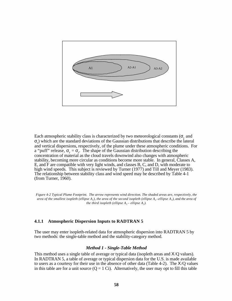
58

Each atmospheric stability class is characterized by two meteorological constants (σy andσz) which are the standard deviations of the Gaussian distributions that describe the lateraland vertical dispersions, respectively, of the plume under these atmospheric conditions. Fora “puff” release, σy = σz. The shape of the Gaussian distribution describing theconcentration of material as the cloud travels downwind also changes with atmosphericstability, becoming more circular as conditions become more stable. In general, Classes A,E, and F are compatible with very light winds, and classes B, C, and D, with moderate tohigh wind speeds. This subject is reviewed by Turner (1977) and Till and Meyer (1983). The relationship between stability class and wind speed may be described by Table 4-1(from Turner, 1960).

Figure 4-2 Typical Plume Footprint. The arrow represents wind direction. The shaded areas are, respectively, thearea of the smallest isopleth (ellipse A1), the area of the second isopleth (ellipse A2 –ellipse A1), and the area of

the third isopleth (ellipse A3 – ellipse A2).

4.1.1 Atmospheric Dispersion Inputs to RADTRAN 5

The user may enter isopleth-related data for atmospheric dispersion into RADTRAN 5 bytwo methods: the single-table method and the stability-category method.

Method 1 - Single-Table MethodThis method uses a single table of average or typical data (isopleth areas and Χ/Q values). In RADTRAN 5, a table of average or typical dispersion data for the U.S. is made availableto users as a courtesy for their use in the absence of other data (Table 4-2). The Χ/Q valuesin this table are for a unit source (Q = 1 Ci). Alternatively, the user may opt to fill this table

A1 A2-A1 A3-A2

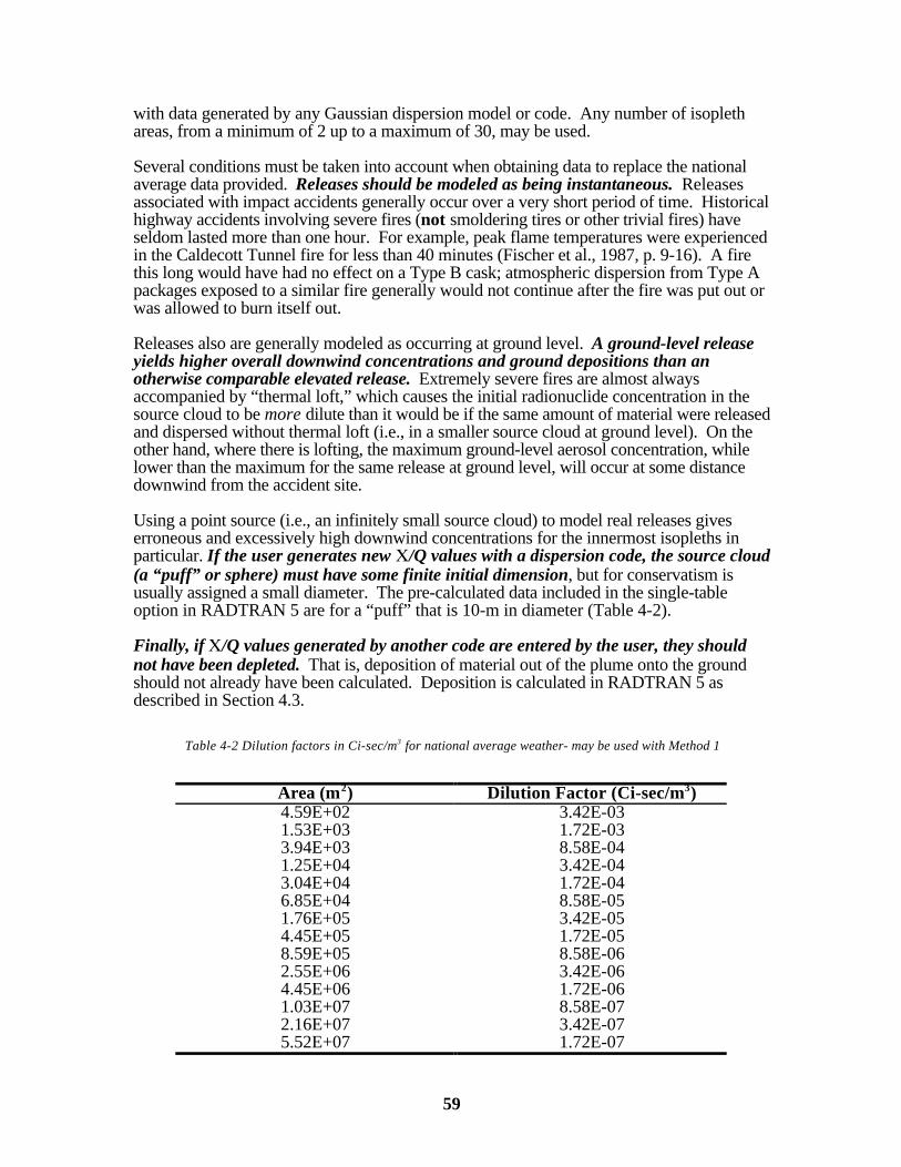
59

with data generated by any Gaussian dispersion model or code. Any number of isoplethareas, from a minimum of 2 up to a maximum of 30, may be used.

Several conditions must be taken into account when obtaining data to replace the nationalaverage data provided. Releases should be modeled as being instantaneous. Releasesassociated with impact accidents generally occur over a very short period of time. Historicalhighway accidents involving severe fires (not smoldering tires or other trivial fires) haveseldom lasted more than one hour. For example, peak flame temperatures were experiencedin the Caldecott Tunnel fire for less than 40 minutes (Fischer et al., 1987, p. 9-16). A firethis long would have had no effect on a Type B cask; atmospheric dispersion from Type Apackages exposed to a similar fire generally would not continue after the fire was put out orwas allowed to burn itself out.

Releases also are generally modeled as occurring at ground level. A ground-level releaseyields higher overall downwind concentrations and ground depositions than anotherwise comparable elevated release. Extremely severe fires are almost alwaysaccompanied by “thermal loft,” which causes the initial radionuclide concentration in thesource cloud to be more dilute than it would be if the same amount of material were releasedand dispersed without thermal loft (i.e., in a smaller source cloud at ground level). On theother hand, where there is lofting, the maximum ground-level aerosol concentration, whilelower than the maximum for the same release at ground level, will occur at some distancedownwind from the accident site.

Using a point source (i.e., an infinitely small source cloud) to model real releases giveserroneous and excessively high downwind concentrations for the innermost isopleths inparticular. If the user generates new /Q values with a dispersion code, the source cloud(a “puff” or sphere) must have some finite initial dimension, but for conservatism isusually assigned a small diameter. The pre-calculated data included in the single-tableoption in RADTRAN 5 are for a “puff” that is 10-m in diameter (Table 4-2).

Finally, if /Q values generated by another code are entered by the user, they shouldnot have been depleted. That is, deposition of material out of the plume onto the groundshould not already have been calculated. Deposition is calculated in RADTRAN 5 asdescribed in Section 4.3.

Table 4-2 Dilution factors in Ci-sec/m3 for national average weather- may be used with Method 1

Area (m2) Dilution Factor (Ci-sec/m3)4.59E+02 3.42E-031.53E+03 1.72E-033.94E+03 8.58E-041.25E+04 3.42E-043.04E+04 1.72E-046.85E+04 8.58E-051.76E+05 3.42E-054.45E+05 1.72E-058.59E+05 8.58E-062.55E+06 3.42E-064.45E+06 1.72E-061.03E+07 8.58E-072.16E+07 3.42E-075.52E+07 1.72E-07

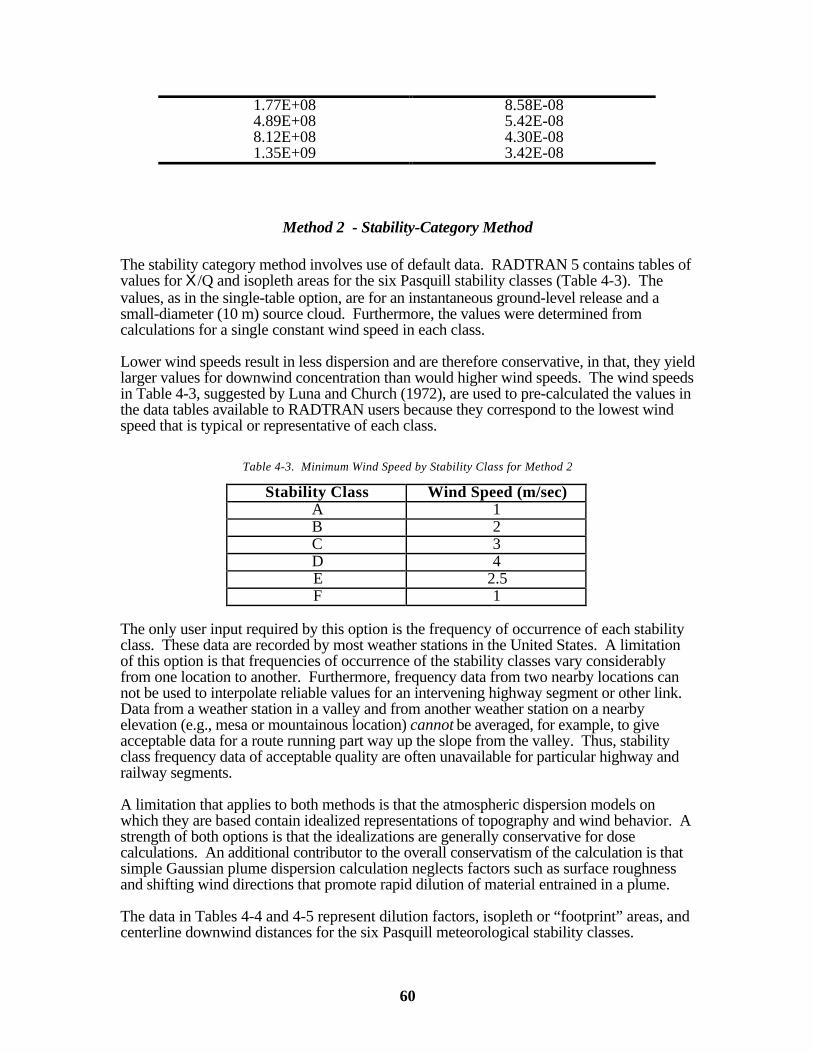
60

1.77E+08 8.58E-084.89E+08 5.42E-088.12E+08 4.30E-081.35E+09 3.42E-08

Method 2 - Stability-Category Method

The stability category method involves use of default data. RADTRAN 5 contains tables ofvalues for Χ/Q and isopleth areas for the six Pasquill stability classes (Table 4-3). Thevalues, as in the single-table option, are for an instantaneous ground-level release and asmall-diameter (10 m) source cloud. Furthermore, the values were determined fromcalculations for a single constant wind speed in each class.

Lower wind speeds result in less dispersion and are therefore conservative, in that, they yieldlarger values for downwind concentration than would higher wind speeds. The wind speedsin Table 4-3, suggested by Luna and Church (1972), are used to pre-calculated the values inthe data tables available to RADTRAN users because they correspond to the lowest windspeed that is typical or representative of each class.

Table 4-3. Minimum Wind Speed by Stability Class for Method 2

Stability Class Wind Speed (m/sec)A 1B 2C 3D 4E 2.5F 1

The only user input required by this option is the frequency of occurrence of each stabilityclass. These data are recorded by most weather stations in the United States. A limitationof this option is that frequencies of occurrence of the stability classes vary considerablyfrom one location to another. Furthermore, frequency data from two nearby locations cannot be used to interpolate reliable values for an intervening highway segment or other link. Data from a weather station in a valley and from another weather station on a nearbyelevation (e.g., mesa or mountainous location) cannot be averaged, for example, to giveacceptable data for a route running part way up the slope from the valley. Thus, stabilityclass frequency data of acceptable quality are often unavailable for particular highway andrailway segments.

A limitation that applies to both methods is that the atmospheric dispersion models onwhich they are based contain idealized representations of topography and wind behavior. Astrength of both options is that the idealizations are generally conservative for dosecalculations. An additional contributor to the overall conservatism of the calculation is thatsimple Gaussian plume dispersion calculation neglects factors such as surface roughnessand shifting wind directions that promote rapid dilution of material entrained in a plume.

The data in Tables 4-4 and 4-5 represent dilution factors, isopleth or “footprint” areas, andcenterline downwind distances for the six Pasquill meteorological stability classes.

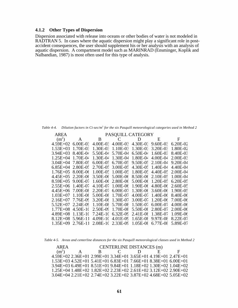
61

4.1.2 Other Types of DispersionDispersion associated with release into oceans or other bodies of water is not modeled inRADTRAN 5. In cases where the aquatic dispersion might play a significant role in post-accident consequences, the user should supplement his or her analysis with an analysis ofaquatic dispersion. A compartment model such as MARINRAD (Ensminger, Koplik andNalbandian, 1987) is most often used for this type of analysis.

Table 4-4. Dilution factors in Ci-sec/m3 for the six Pasquill meteorological categories used in Method 2

AREA PASQUILL CATEGORY(m2) A B C D E F

4.59E+02 6.00E-03 4.00E-03 4.00E-03 4.30E-03 9.60E-03 6.20E-021.53E+03 1.70E-03 1.30E-03 1.10E-03 1.30E-03 3.20E-03 1.80E-023.94E+03 8.40E-04 5.50E-04 5.70E-04 6.50E-04 1.60E-03 8.40E-031.25E+04 1.70E-04 1.30E-04 1.30E-04 1.80E-04 4.00E-04 2.00E-033.04E+04 7.80E-05 6.00E-05 6.70E-05 9.50E-05 2.10E-04 9.20E-046.85E+04 2.80E-05 2.70E-05 3.00E-05 4.30E-05 1.40E-04 4.40E-041.76E+05 8.00E-06 1.00E-05 1.00E-05 1.80E-05 4.40E-05 2.00E-044.45E+05 2.20E-06 3.50E-06 5.00E-06 8.50E-06 2.10E-05 1.00E-048.59E+05 9.00E-07 1.60E-06 2.80E-06 5.00E-06 1.20E-05 6.20E-052.55E+06 1.40E-07 4.10E-07 1.00E-06 1.90E-06 4.80E-06 2.60E-054.45E+06 7.00E-08 2.20E-07 6.00E-07 1.30E-06 3.60E-06 1.90E-051.03E+07 1.10E-08 5.00E-08 1.70E-07 4.00E-07 1.40E-06 8.40E-062.16E+07 7.76E-09 3.20E-08 1.30E-07 3.00E-07 1.20E-06 7.00E-065.52E+07 2.24E-09 1.10E-08 5.70E-08 1.50E-07 6.00E-07 4.00E-061.77E+08 4.50E-10 2.50E-09 1.70E-08 5.50E-08 2.80E-07 2.00E-064.89E+08 1.13E-10 7.24E-10 6.32E-09 2.41E-08 1.38E-07 1.09E-068.12E+08 5.96E-11 4.09E-10 4.01E-09 1.65E-08 9.97E-08 8.22E-071.35E+09 2.76E-11 2.08E-10 2.33E-09 1.05E-08 6.77E-08 5.89E-07

Table 4-5. Areas and centerline distances for the six Pasquill meteorological classes used in Method 2

AREA CENTERLINE DISTANCES (m)(m2) A B C D E F

4.59E+02 2.36E+01 2.99E+01 3.34E+01 3.65E+01 4.19E+01 2.47E+011.53E+03 4.52E+01 5.41E+01 6.83E+01 7.66E+01 8.38E+01 6.00E+013.94E+03 6.49E+01 8.51E+01 9.84E+01 1.18E+02 1.30E+02 1.04E+021.25E+04 1.48E+02 1.82E+02 2.23E+02 2.61E+02 3.12E+02 2.90E+023.04E+04 2.21E+02 2.74E+02 3.22E+02 3.87E+02 4.68E+02 5.05E+02

62

6.85E+04 3.74E+02 4.17E+02 5.03E+02 6.33E+02 6.05E+02 8.57E+021.76E+05 5.89E+02 7.04E+02 9.25E+02 1.09E+03 1.26E+03 1.51E+034.45E+05 8.99E+02 1.23E+03 1.36E+03 1.73E+03 2.00E+03 2.48E+038.59E+05 1.21E+03 1.85E+03 1.87E+03 2.40E+03 2.85E+03 3.49E+032.55E+06 2.22E+03 3.80E+03 3.31E+03 4.37E+03 5.09E+03 6.51E+034.45E+06 2.78E+03 5.27E+03 4.40E+03 5.53E+03 6.11E+03 8.15E+031.03E+07 5.11E+03 1.15E+04 8.85E+03 1.15E+04 1.19E+04 1.46E+042.16E+07 5.71E+03 1.46E+04 1.03E+04 1.37E+04 1.35E+04 1.67E+045.52E+07 8.65E+03 2.56E+04 1.62E+04 2.11E+04 2.37E+04 2.49E+041.77E+08 1.46E+04 5.59E+04 3.17E+04 3.92E+04 4.39E+04 4.09E+044.89E+08 2.31E+04 1.08E+05 5.50E+04 6.56E+04 7.70E+04 6.29E+048.12E+08 2.82E+04 1.45E+05 7.07E+04 8.12E+04 1.01E+05 7.76E+041.35E+09 3.62E+04 2.06E+05 9.61E+04 1.06E+05 1.38E+05 9.71E+04

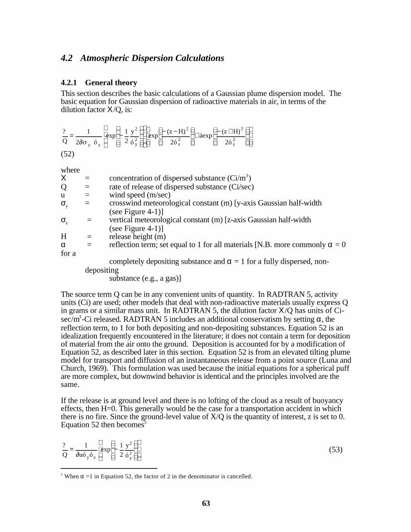
63

4.2 Atmospheric Dispersion Calculations

4.2.1 General theoryThis section describes the basic calculations of a Gaussian plume dispersion model. Thebasic equation for Gaussian dispersion of radioactive materials in air, in terms of thedilution factor Χ/Q, is:

+−+

−−

−=2z

2

2z

2

2y

2

zy 2ó

H)(záexp

2ó

H)(zexp

ó

y

2

1exp

ó2∂1

Q

?

(52)

whereΧ = concentration of dispersed substance (Ci/m3)Q = rate of release of dispersed substance (Ci/sec)u = wind speed (m/sec)σy = crosswind meteorological constant (m) [y-axis Gaussian half-width

(see Figure 4-1)]σz = vertical meteorological constant (m) [z-axis Gaussian half-width

(see Figure 4-1)]H = release height (m)α = reflection term; set equal to 1 for all materials [N.B. more commonly α = 0for a

completely depositing substance and α = 1 for a fully dispersed, non-depositing

substance (e.g., a gas)]

The source term Q can be in any convenient units of quantity. In RADTRAN 5, activityunits (Ci) are used; other models that deal with non-radioactive materials usually express Qin grams or a similar mass unit. In RADTRAN 5, the dilution factor Χ/Q has units of Ci-sec/m3-Ci released. RADTRAN 5 includes an additional conservatism by setting α, thereflection term, to 1 for both depositing and non-depositing substances. Equation 52 is anidealization frequently encountered in the literature; it does not contain a term for depositionof material from the air onto the ground. Deposition is accounted for by a modification ofEquation 52, as described later in this section. Equation 52 is from an elevated tilting plumemodel for transport and diffusion of an instantaneous release from a point source (Luna andChurch, 1969). This formulation was used because the initial equations for a spherical puffare more complex, but downwind behavior is identical and the principles involved are thesame.

If the release is at ground level and there is no lofting of the cloud as a result of buoyancyeffects, then H=0. This generally would be the case for a transportation accident in whichthere is no fire. Since the ground-level value of X/Q is the quantity of interest, z is set to 0. Equation 52 then becomes5

−=2y

2

zy ó

y

2

1exp

ó∂uó

1

Q

? (53)

5 When α =1 in Equation 52, the factor of 2 in the denominator is cancelled.

64

Figures 4-3a and 4-3b (from Turner, 1969) show the relationship between σy and σz anddownwind distance. From the figures, it is evident that Χ/Q decreases rapidly as one moveslaterally away from the plume centerline. The “footprint” of the plume, shownschematically in Figure 4-2 is thus an ellipse with the semi-major axis in the direction of thewind and a relatively small semi-minor axis. As meteorological stability increases fromClass A to Class F, σy decreases and the semi-minor axis lengthens relative to the semi-major axis, yielding a shorter, “fatter” footprint. The ellipses of Figure 4-2 are isopleths –curves of constant Χ/Q that may be obtained by solving Equation 53 for each Pasquillstability class for different values of downwind and crosswind distance. Both σy and σz arefunctions of the downwind distance. The areas in Tables 4-3 and 4-4 are the areas insidethe isopleths.

At ground level along the plume centerline (y=0), Equation 53 reduces to

zyó∂uó1

Q? =

(54)

Deposition of particles from an airborne plume is calculated by incorporating the depositionvelocity of the particle, Vd (m/sec), into Equation 54, which yields:

zy

d

ó∂uó

V

Q

? =

(55)

In Equations 54 and 55, Χ/Q is expressed in units of Ci/m2-Ci released. The RADTRANuser can substitute Χ/Q values and footprint areas for an elevated release, if desired, by off-line calculation with Equation 53.

−

−=2z

2

2y

2

zy 2ó

Hexp

2ó

yexp

ó∂uó

1

Q

?

(56)where all variables are previously defined.

If user-generated isopleths for the case of deposition only are substituted, then α = 0 andEquation 56 becomes

−

−=2z

2

2y

2

y 2ó

Hexp

2ó

yexp

u2

1

Q

?

z

(57)where all variables are previously defined.

Calculation of deposition requires incorporation of the settling velocity into Equation 57,6

which yields:

6 For a derivation of this equation see Chapter 5, Sections 5.5 and 5.6 of Wark and Warner (1981).

65

−

−

−=2

z

d

2y

2

y

d

2ó

u

xVH

exp2ó

yexp

u2

V

Q

?

z

(58)

where x is the downwind distance along the plume centerline (m) and all other variables areas previously defined.

66

Figure 4-3a. Crosswind Gaussian half-width ( y) as a function of downwind distance and meteorological stability. A, B, C, D, E, and F are the six Pasquill meteorological stability classes. From Turner (1969) as cited in Wark andWarner, (1981).

1.E+00

1.E+01

1.E+02

1.E+03

1.E+04

0.1 0.2 0.4 0.7 1 2 4 7 10 20

Kilometers Downwind

sig

ma

(y)

-- m

eter

s

A

BCD

EF

67

Figure 4-3b. Vertical Gaussian half-width ( z) as a function of downwind distance and meteorological stability. A,B, C, D, E, and F are the six Pasquill meteorological stability classes. From Turner (1969) as cited in Wark andWarner, 1981).

1.E+00

1.E+01

1.E+02

1.E+03

1.E+04

0.1 0.2 0.4 0.7 1 2 4 7 10 20

Kilometers Downwind

Sig

ma(

z) -

- m

eter

s

A

B CD

E

F

68

4.3 RADTRAN Calculations

4.3.1 Input DataIn RADTRAN 5, either Table 4-2 or Table 4-4 or an appropriate user-generatedsubstitution, is used as input data. Advantage is taken of the fact that for a unit release (Q =1 Ci), Χ/Q is equal to Χ. The remaining discussion applies to a unit release. For eachmeteorological stability class, the value of Χ at the downwind edge of A1 is initially taken tobe Χ (from the top line of Table 4-2 or Table 4-4) and set equal to 1Χ . The area of the firstisopleth A1 must be small, so that the resulting underestimate of 1Χ will not be significant. The initial value of Χ for other isopleth areas is also taken to be the value Χ at thedownwind end of the area.

The dilution factor for the area A2-A1 (see Figure 4-2) is the geometric mean of the largestand smallest dilution factors for that area:

1202 ?? ? −=

(59)

The nth dilution factor is thus

1-nn0n Χ−Χ=Χ

(60)

Equations 59 and 60 are used in RADTRAN 5 for non-depositing materials (e.g., gases). Deposition velocity is introduced into the calculation in two places, as described below.

4.3.2 First introduction of Vd

The amount deposited (Ci/m2) in the first isopleth area 01DEP is:

1d1

__0

1 AV?DEP ⋅⋅= (61)whereΧ = concentration of dispersed material (Ci/m3)Vd = deposition velocity (m/s)A1 = isopleth area (m2).

The amount of material deposited in the nth area, n≥2, is

[ ]1nndn

__0n AAV?DEP −−⋅⋅=

(62)

where all variables are previously defined.

The total amount of material deposited out to An is then

∑=

+=n

2i

0i

01

0n DEPDEPDEP

(63)

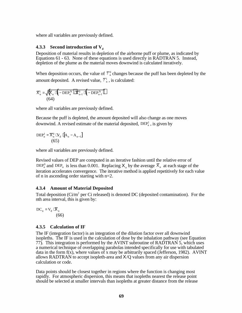
69

where all variables are previously defined.

4.3.3 Second introduction of Vd

Deposition of material results in depletion of the airborne puff or plume, as indicated byEquations 61 - 63. None of these equations is used directly in RADTRAN 5. Instead,depletion of the plume as the material moves downwind is calculated iteratively.

When deposition occurs, the value of 0n? changes because the puff has been depleted by the

amount deposited. A revised value, 1n? , is calculated:

( ) ( )( )N1-n

01-n

Nnn

1n DEP1DEP1 −⋅Χ⋅−⋅Χ=Χ

(64)

where all variables are previously defined.

Because the puff is depleted, the amount deposited will also change as one movesdownwind. A revised estimate of the material deposited, 1

nDEP , is given by

[ ]1nnd0n

1n AAVDEP −−⋅⋅Χ=

(65)

where all variables are previously defined.

Revised values of DEP are computed in an iterative fashion until the relative error of0nDEP and nDEP is less than 0.001. Replacing Χn by the average nΧ at each stage of the

iteration accelerates convergence. The iterative method is applied repetitively for each valueof n in ascending order starting with n=2.

4.3.4 Amount of Material DepositedTotal deposition (Ci/m2 per Ci released) is denoted DC (deposited contamination). For thenth area interval, this is given by:

ndn V DC Χ⋅= (66)

4.3.5 Calculation of IFThe IF (integration factor) is an integration of the dilution factor over all downwindisopleths. The IF is used in the calculation of dose by the inhalation pathway (see Equation77). This integration is performed by the AVINT subroutine of RADTRAN 5, which usesa numerical technique of overlapping parabolas intended specifically for use with tabulateddata in the form f(x), where values of x may be arbitrarily spaced (Jefferson, 1982). AVINTallows RADTRAN to accept isopleth-area and Χ/Q values from any air dispersioncalculation or code.

Data points should be closest together in regions where the function is changing mostrapidly. For atmospheric dispersion, this means that isopleths nearest the release pointshould be selected at smaller intervals than isopleths at greater distance from the release

70

point.7 Thus, when isopleths are selected so that A1 of Figure 4-3 is relatively small,underestimation of 1Χ will be minimal. The only constraints on isopleth selection are thoseimposed by the AVINT subroutine:• Each isopleth area should be at least 6% larger than the preceding area;

• Each isopleth area should be no more than 4 times larger than the preceding area; and

• Since AVINT requires at least two data pairs, input data for at least two isopleth areasmust be entered (if only a single pair of dispersion parameters is entered, then an errormessage appears and the calculation does not proceed).

7 If data points are spaced too far apart, the AVINT routine will produce incorrect results. The user intending to

generate problem-specific dispersion data is directed to Jefferson (1982) for more information.

71

5 CALCULATION OF ACCIDENT DOSES ANDDOSE-RISKS

5.1 Introduction to Accident Consequence Calculations

Radiation dose is the primary consequence calculated with RADTRAN 5. Dose values aremultiplied by probabilities to yield dose-risk values. Varying types of accident havevarying consequences. The following sections describe how accidents are categorized bydose level and how doses are calculated for the various exposure pathways. Shieldingdamage and actual releases may be modeled separately.

5.1.1 Exposure PathwaysSix potential radiation exposure pathways may be modeled in RADTRAN 5:• Direct Radiation (Loss of Shielding)• Cloudshine• Inhalation• Groundshine• Resuspension• Ingestion.

5.1.2 Accident Severity and Package ResponseIn RADTRAN 5, the spectrum of accidents is described in terms of package response. Theuser may define up to 30 accident-severity categories. Accident categorization is somewhatflexible. Most commonly, each category represents all transportation accident outcomesthat result in a specified package response, regardless of how that response is elicited. However, differing means of arriving at the same outcome may also be treated separately. Severity-categories are best derived by means of event-tree analysis, and the RADTRANapproach allows several branches of an event tree that lead to a similar package response tobe grouped together and their probabilities summed.

For a given level of package response, actual releases, if any, are determined in part by thephysical-chemical properties of the contents. Technically, the term “release” isdistinguished from the term “loss of shielding” (LOS) by the fact that in the former somepart of the contents is expelled from the packaging. However, any scenario in which someor all of the contents of a package merely end up outside the packaging, without downwinddispersal of particulates, should be treated as a LOS event because it involves an unshieldedsource. Only when material is dispersed away from the immediate vicinity of theaccident are dispersion models and pathways appropriate. When material is released ingaseous or aerosol form, then the atmospheric-dispersion calculations discussed in Chapter4 are used to estimate downwind concentrations and depositions of the material onto theground.

5.1.3 Dose Calculation OutlineConsequences are calculated in a step-wise fashion. The first step is to develop anexpression for an individual dose or dose rate for a particular exposure pathway. Forexample, a general expression for inhalation dose to an individual in the nth downwindisopleth for an accident of severity j is developed. This expression is then multiplied by thetotal number of persons in the same dose group [i.e., the product of the area (An – An-1 in

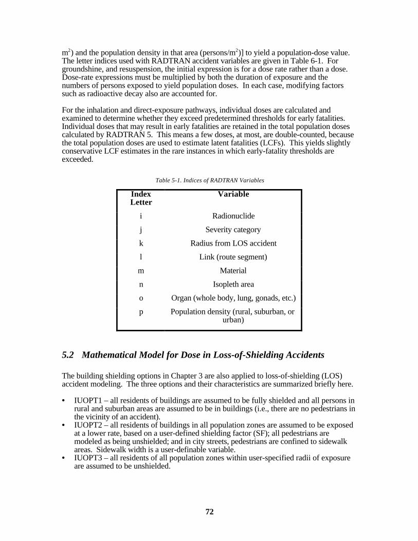
72

m2) and the population density in that area (persons/m2)] to yield a population-dose value. The letter indices used with RADTRAN accident variables are given in Table 6-1. Forgroundshine, and resuspension, the initial expression is for a dose rate rather than a dose. Dose-rate expressions must be multiplied by both the duration of exposure and thenumbers of persons exposed to yield population doses. In each case, modifying factorssuch as radioactive decay also are accounted for.

For the inhalation and direct-exposure pathways, individual doses are calculated andexamined to determine whether they exceed predetermined thresholds for early fatalities. Individual doses that may result in early fatalities are retained in the total population dosescalculated by RADTRAN 5. This means a few doses, at most, are double-counted, becausethe total population doses are used to estimate latent fatalities (LCFs). This yields slightlyconservative LCF estimates in the rare instances in which early-fatality thresholds areexceeded.

Table 5-1. Indices of RADTRAN Variables

IndexLetter

Variable

i Radionuclide

j Severity category

k Radius from LOS accident

l Link (route segment)

m Material

n Isopleth area

o Organ (whole body, lung, gonads, etc.)

p Population density (rural, suburban, or urban)

5.2 Mathematical Model for Dose in Loss-of-Shielding Accidents

The building shielding options in Chapter 3 are also applied to loss-of-shielding (LOS)accident modeling. The three options and their characteristics are summarized briefly here.

• IUOPT1 – all residents of buildings are assumed to be fully shielded and all persons inrural and suburban areas are assumed to be in buildings (i.e., there are no pedestrians inthe vicinity of an accident).

• IUOPT2 – all residents of buildings in all population zones are assumed to be exposedat a lower rate, based on a user-defined shielding factor (SF); all pedestrians aremodeled as being unshielded; and in city streets, pedestrians are confined to sidewalkareas. Sidewalk width is a user-definable variable.

• IUOPT3 – all residents of all population zones within user-specified radii of exposureare assumed to be unshielded.

73

In many cases, the vast majority of the radionuclide inventory of a package will notcontribute to the LOS source strength because of self-shielding, regardless of how muchshielding is degraded. Modeling of such materials is discussed in Section 5.2.3.

5.2.1 LOS Gamma Dose for Small PackagesThe following dose-rate formula, which is adapted from Equation (1) for a uniformlyradiating source may be used to calculate gamma dose for LOS accidents involving smallpackages.

2

rì

gr

r)B(e EFPPSCi Q(r)DR

⋅⋅⋅⋅⋅⋅=−

(67)

whereDRg(r ) = gamma dose rate at distance r (mrem/hr)Q = units conversion constantCi = number of curies per packagePPS = number of packages per shipmentEF = exposure fraction (see Section)ε = photon energy (Mev)µ = linear absorption coefficient (m-1)B(µr) = dose-rate buildup factorr = distance from source (m)

For gamma radiation, the simplifying assumption that [e-µr ⋅ B(r)] = 1.0 reduces theexpression to

2k

iji,ml,i6ml,k,j,i,g

r

EFPPSCiQ(r)DR

⋅⋅⋅⋅=

(68)

whereDRg(r ) = gamma dose rate at distance r (mrem/hr)Q6 = 0.5 rem-m/hr-Ci-MevCii = number of curies of isotope iPPS l,m = number of packages of material m traveling on link lEFi,j = exposure fraction of isotope i in severity category j (see next section)εi = photon energy of isotope i (Mev)rk = radial distance from source to annular area k (meters); rk = RADISTk –RADISTk-1

for k = 2...NRAD; r1 defines the innermost circle (exclusion area)

Drivers of cars potentially caught in a traffic jam near a LOS accident in highway mode arenot modeled separately. The pedestrian (unshielded) population in the innermost annulus(first term in brackets in Equation 69 below) is adjusted with the RPD (ratio of pedestriandensity to baseline population density) because it is assumed the first annulus encompassespedestrian walkways or sidewalks adjacent to the roadway. Persons at greater distances arerepresented as enjoying some degree of shielding from intervening buildings, automobiles,etc., which is accounted for by assigning appropriate values to the SF (shielding fraction)coefficient in the second term.

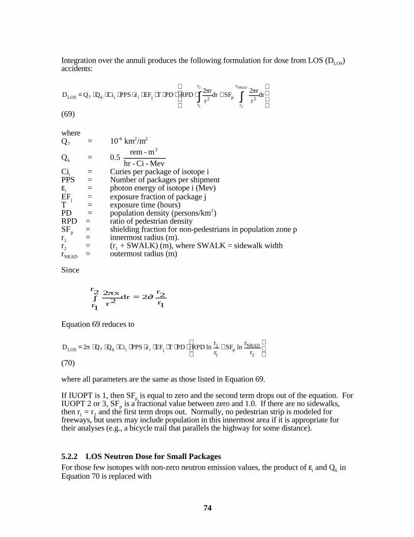
74

Integration over the annuli produces the following formulation for dose from LOS (DLOS)accidents:

+⋅⋅⋅⋅⋅⋅⋅⋅⋅= ∫∫ dr

r

r2 SFdr

r

r2 RPDPD TEF PPS Ci QQ D

NRAD

2

2

1

r

r2p

r

r2ji67LOS i

(69)

whereQ7 = 10-6 km2/m2

Q6 = 0.5 Mev-Ci-hr

m-rem 2

Cii = Curies per package of isotope iPPS = Number of packages per shipmentεi = photon energy of isotope i (Mev)EFj = exposure fraction of package jT = exposure time (hours)PD = population density (persons/km2)RPD = ratio of pedestrian densitySFp = shielding fraction for non-pedestrians in population zone pr1 = innermost radius (m).r2 = (r1 + SWALK) (m), where SWALK = sidewalk widthrNRAD = outermost radius (m)

Since

Equation 69 reduces to

+⋅⋅⋅⋅⋅⋅⋅⋅⋅=

2

NRADp

1

2ji67LOS r

rln SF

r

rln RPDPD T EF PPS Ci QQ2 D i

(70)

where all parameters are the same as those listed in Equation 69.

If IUOPT is 1, then SFp is equal to zero and the second term drops out of the equation. ForIUOPT 2 or 3, SFp is a fractional value between zero and 1.0. If there are no sidewalks,then r1 = r2 and the first term drops out. Normally, no pedestrian strip is modeled forfreeways, but users may include population in this innermost area if it is appropriate fortheir analyses (e.g., a bicycle trail that parallels the highway for some distance).

5.2.2 LOS Neutron Dose for Small PackagesFor those few isotopes with non-zero neutron emission values, the product of εi and Q6 inEquation 70 is replaced with

1r2

r2∂dr

2r

1r2r

x2=∫

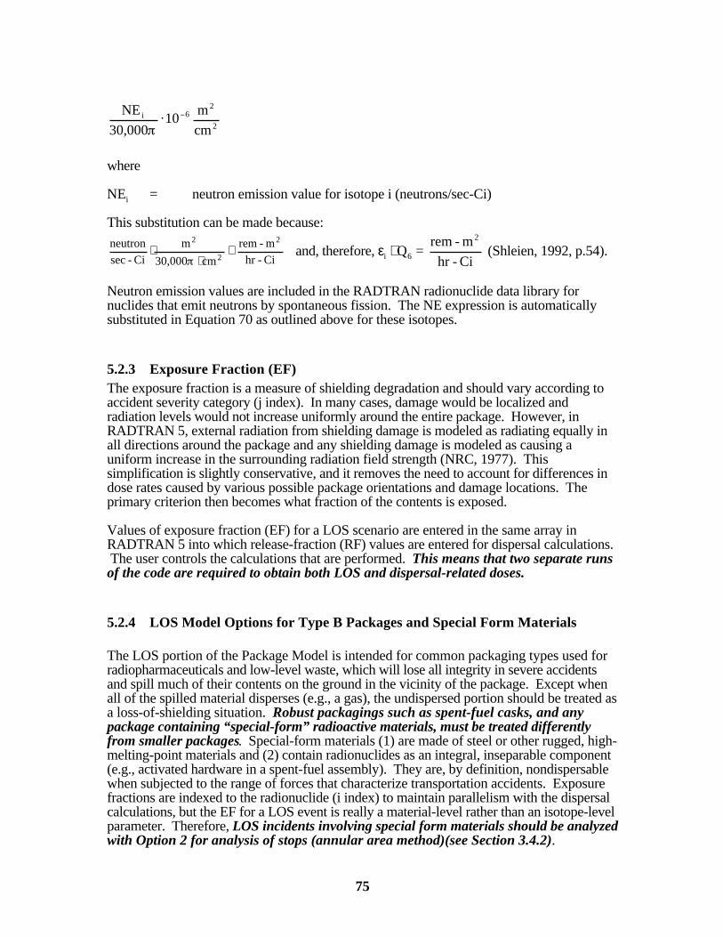
75

2

26i

cm

m10

30,000

NE

where

NEi = neutron emission value for isotope i (neutrons/sec-Ci)

This substitution can be made because:

Ci-hr

m-rem

cm30,000

m

Ci-sec

neutron 2

2

2

≅⋅

⋅ and, therefore, εi ⋅ Q6 = Ci-hr

m-rem 2

(Shleien, 1992, p.54).

Neutron emission values are included in the RADTRAN radionuclide data library fornuclides that emit neutrons by spontaneous fission. The NE expression is automaticallysubstituted in Equation 70 as outlined above for these isotopes.

5.2.3 Exposure Fraction (EF)The exposure fraction is a measure of shielding degradation and should vary according toaccident severity category (j index). In many cases, damage would be localized andradiation levels would not increase uniformly around the entire package. However, inRADTRAN 5, external radiation from shielding damage is modeled as radiating equally inall directions around the package and any shielding damage is modeled as causing auniform increase in the surrounding radiation field strength (NRC, 1977). Thissimplification is slightly conservative, and it removes the need to account for differences indose rates caused by various possible package orientations and damage locations. Theprimary criterion then becomes what fraction of the contents is exposed.

Values of exposure fraction (EF) for a LOS scenario are entered in the same array inRADTRAN 5 into which release-fraction (RF) values are entered for dispersal calculations. The user controls the calculations that are performed. This means that two separate runsof the code are required to obtain both LOS and dispersal-related doses.

5.2.4 LOS Model Options for Type B Packages and Special Form Materials

The LOS portion of the Package Model is intended for common packaging types used forradiopharmaceuticals and low-level waste, which will lose all integrity in severe accidentsand spill much of their contents on the ground in the vicinity of the package. Except whenall of the spilled material disperses (e.g., a gas), the undispersed portion should be treated asa loss-of-shielding situation. Robust packagings such as spent-fuel casks, and anypackage containing “special-form” radioactive materials, must be treated differentlyfrom smaller packages. Special-form materials (1) are made of steel or other rugged, high-melting-point materials and (2) contain radionuclides as an integral, inseparable component(e.g., activated hardware in a spent-fuel assembly). They are, by definition, nondispersablewhen subjected to the range of forces that characterize transportation accidents. Exposurefractions are indexed to the radionuclide (i index) to maintain parallelism with the dispersalcalculations, but the EF for a LOS event is really a material-level rather than an isotope-levelparameter. Therefore, LOS incidents involving special form materials should be analyzedwith Option 2 for analysis of stops (annular area method)(see Section 3.4.2).

76

With Option 2, persons who might be in the vicinity of a LOS accident are represented asbeing uniformly distributed within a set of annular areas surrounding the accident location. The inner radius of the innermost annular area (r1) must define a circular exclusionarea around the accident location within which there are no people. Beyond this radius,the incremental dose area is given by (2πr)dr. Dose is the product of integration of thisincremental dose area, integrated dose rate, time of exposure, and population density withinthe dose area. The dose rate normally should be the surface dose rate of the special formmaterial or spent fuel that is exposed and may be treated as 100% gamma or entered asgamma and neutron fractions, as desired. If the shielding is only partially compromised orreduced (e.g., lead slump in a steel-lead-steel spent-fuel cask), then the shielding factor(SFst) in the Option 2 stop equation (Equation 41) can be made equivalent to the EF.

5.2.5 Exposure TimesIn rural and suburban areas, the recommended exposure time (T or ∆T) is 0.67 hours; inurban areas, it is 0.42 hour. Exposure time is the sum of the time required for firstresponders to (a) arrive at the accident site, (b) decide on a course of action and (c) movepersons away from the immediate area (Mills, Neuhauser and Smith, 1995).

5.2.6 Early-Effects Calculation

Gamma RadiationA variation of the IUOPT1 model is also used to assess early effects, since only unshieldedpersons (i.e., persons out of doors) located at relatively short distances from a LOS accidentlocation could potentially receive doses above the early-effects thresholds. Exposure time(Texp) is defined as the time elapsed before first responders arrive and establish a cordonaround the accident site.8 If the Option 2 Stop Model is being used to analyze LOSscenarios for large packages, then early effects will not be calculated by RADTRAN 5.

The modifying parameter, RPD (see Chapter 3), is used to estimate the number of personsout of doors for accidents that occur on city streets. The expected number of exposedpersons (EXPk,u) in each annular area on a city street is given by

EXPk, u = Q7 ⋅rk ⋅ SEG ⋅ SWALK ⋅ [RPD ⋅ PDu] (71)

whereQ7 = units conversion factor = 1.0E-6 km2/m2

rk = annular radius for nondispersal accidents defined by input variableRADIST;

rk = RADISTk – RADISTk-1 for k =2...NRAD, where r1 defines theinnermost

circle (the radius of the exclusion area). SWALK = width of segment where pedestrians are located (e.g., sidewalks) (m)

8 The recommended value of Texp in urban areas is ~25 min. Rush hour situations could involve greater response

times, for example, while the presence of an imminent hazard reduces decision time. Thus, Texp is eminentlysuitable for uncertainty analysis by means of Latin Hypercube Sampling (LHS). Mills, Neuhauser and Smith(1995) discuss this topic.

77

SEG = number of segments per annulus = 8RPD = multiplier of PDu that accounts for non-residents (acronym of ratio ofpedestrian density)PDu = urban population density (persons/km2).

For urban areas without sidewalks (e.g., interstate passing through an urban area),

2ku7uk, rRUUBFPDQEXP ⋅⋅⋅⋅⋅=

(72)

where all variables are the same as in Equation 71 except forUBF = fraction of persons indoors (acronym of urban building fraction)RU = building shielding factor for urban areasrk = annular radius for nondispersal accidents defined by input variableRADIST;

2kr = (RADISTk)

2-(RADISTk-1)2

In suburban and rural areas, EXPs and EXPr, are given by

2ksor r 7sor r rPDQEXP ⋅⋅⋅=

(73)

where all variables are the same as in Equations 71 and 72.

The LOS-related dose (DLOS) to the population in the kth annular area is

2k

jii6LOS

r

TEFPPSCiQD

⋅⋅⋅⋅⋅=

(74)

whereQ6 = units conversion factor = 0.5E-06 rem-m2/hr-Ci-MevCii = number of curies of ith isotope (Ci)PPS = number of packages per shipmentεi = photon energy of ith isotope (Mev)T = exposure time (hr)EFj = exposure fraction for accident of severity jrk = annulus radius k for non-dispersal accidents (m)

Neutron RadiationIf one or more neutron emitters are among the isotopes in a package, then Equation 74 ismodified as follows.9

2k

jii8LOS

r30,000

EFTPPSCiNEQD

⋅⋅⋅⋅⋅⋅

=

(75)

9 Note on units:

hr

rem

sec 2cm

neutron ≅⋅

78

whereQ8 = units conversion factor = 1.0E-06 m2/cm2

NEi = neutron emission factor for radionuclide i (neutrons/sec-Ci)Cii = number of curies of ith radionuclide (Ci)PPS = number of packages per shipmentEFj = exposure fraction for accident of severity jT = exposure time (hr)rk = annulus radius k for non-dispersal accidents (m)

5.3 Mathematical Models for Dose in Dispersion Accidents

5.3.1 Mathematical Model for Dose to an Individual from Inhalation of DispersedMaterials

In RADTRAN 5, the average individual inhalation dose attributed to a released amount ofrespirable aerosol of isotope i in material m within each downwind isopleth area, (An-An-1),is computed as follows:

( )BRRPCRESPAER RF PPS CiD noi,ji,ji,ji,Li

organs all

o

desradionucli all

i

materials all

minh ⋅Χ⋅⋅⋅⋅⋅⋅= ∑∑∑

(76)

whereDinh = individual inhalation dose (rem)Cii = number of curies of isotope i in package (Ci)PPSL = number of packages on link LRFi,j = fraction of package contents released in accident of severity jAERi,j = fraction of released material that is in aerosol form in accident of severity jRESPi,j = fraction of aerosol material that is respirable in accident of severity jRPCi,o = dose conversion factor (rem per Ci) for ith isotope and oth organ (lung,marrow,

and thyroid)nΧ = dilution factor (chi) in nth isopleth area (Ci-sec/m3 per Ci released; see

Chapter 4)BR = breathing rate (m3/sec)

5.3.2 Derivation of Mathematical Model for Integrated Population Dose fromDirect Inhalation of Dispersed Material

The integrated population dose ( popinhD ) from direct inhalation following a release of material

in aerosol form is given by

nLiji,ji,ji,Li7popinh APDBR IF RPC RESP AERRFPPS Ci Q D ⋅⋅⋅⋅⋅⋅⋅⋅⋅⋅=

(77)

where,Q7 = units conversion factor = 10-6 km2/m2

Cii = number of curies of radionuclide i per package (Ci)

79

PPSL = number of packages per shipment on link LRFi,j = release fraction of radionuclide i in accident of severity jAERi,j = fraction of released radionuclide i that is aerosol in accident of severity jRESPi,j = fraction of aerosolized radionuclide i that is respirable in accident of severityjRPCi = dose conversion factor for radionuclide i (rem per curie inhaled)10

IF = integral of time-integrated atmospheric dilution factors, Χ, over all downwindareas

BR = breathing rate (m3/min)PDL = population density on link L (persons/km2)An = area of nth isopleth (m2)

The calculation of IF is described in Chapter 4. In urban areas, persons inside and personsoutside of buildings may accumulate inhalation dose. To account for this, the populationdensity term in Equation 77 is multiplied by the following term:

[(UBF ⋅ BDF) + (USWF ⋅ RPD)]whereUBF = fraction of persons indoors (or urban building fraction)BDF = building dose factorUSWF= fraction of persons out of doors (or urban sidewalk fraction)RPD = ratio of pedestrian density to residential density.

The reasons this term is used are:(1) For persons in buildings, an additional measure of protection is provided by the

structure itself (Engelmann, 1990). This effect is accounted for by a Building DoseFactor (BDF).

(2) The total number of persons located in buildings in an urban area is modeled as theproduct of the potentially exposed population and the Urban Building Fraction (UBF),which is the fraction of the population in buildings.11 Thus, the first term in theexpression (UBF⋅BDF), acts as a modifier of the product of population density (PDu)and area (An) and yields number of persons in buildings, who are exposed a lower rateaccording to the value of BDF.

(3) Persons out of doors (USWF) are modeled as being completely unshielded. While thisis a user-supplied input value, it should equal 1 – UBF.

(4) The Pedestrian Density Ratio (RPD) is the ratio of pedestrian density to residentialdensity. It is used to account for persons out of doors who are not residents (e.g.,shoppers). It is used as a multiplier of the basic urban population density. The RPD isa user-supplied value, but city-specific data are difficult to obtain. The default value of 6is from New York City (Finley et al., 1980) and is likely to be conservative for manyother urban areas.

The basic inhalation dose calculation can also be manipulated to yield dose to persons inenclosed spaces. This specialized technique was developed to examine potential doses topersons onboard an aircraft from a hypothetical leaking radioactive materials container(Neuhauser, 1992).

10 May be reset to zero for special-form materials with the DEFINE function of RADTRAN 5.

11 In previous releases of RADTRAN, this variable was defined as the fraction of the urban area occupied bybuildings, but new GIS-based methods of determining population density already account for the unequaldistribution of population within the urban area, and UBF + USWF should equal 1.

80

5.3.3 Derivation of Mathematical Models for Integrated Population Dose fromResuspension

Population dose via the inhalation pathway may also result from deposited materialsbecause particulates can be resuspended by various mechanisms, such as wind, andsubsequently be inhaled. The additional dose from this exposure pathway is accounted forby using a Resuspension Dose Factor (RDF). The RDF is a nondimensional factor that isapplied to the direct inhalation dose. Resuspension dose (Dres) can thus be expressed as

( )1-RDFD D inhres ⋅= , (78)

whereDinh = direct inhalation dose (from Equation 77)RDF = resuspension dose factor

The resuspension dose factor is a nondimensional value that is applied to the inhalationdose, following NRC, 1975.

( ) ( ) ( )

−+−⋅+=

−−21 18250-

2

918250-

1

54

d e110

e110

x1064.8V 1 RDF

(79)

whereVd = deposition velocity (m/sec)λ1 = 0.693[1/RT1/2 + 1/t1/2]λ2 = 0.693/t1/2

RT1/2 = resuspension half-life (days)t1/2 = radioactive half-life (days).

For consistency with other RADTRAN dose models, a value of 50 years (18250 days) isused for the period of dose integration. The resuspension half-life is set to 365 days (NRC,1975) and the radioactive half-life is radionuclide-specific.

5.3.4 Mathematical Model for Integrated Population Dose from Cloudshine

Cloudshine is defined as radiation emitted directly by airborne particulates. As a generalrule, cloudshine dose is not large and seldom contributes significantly to totaltransportation-accident dose (Finley et al., 1980). However, dose from an aerosol release ofcertain radionuclides could be significant, particularly those that emit high-photon-energygamma radiation such as 24Na and 60Co, which are used in radiomedicine. CloudshineDose Factors (CDFs) are calculated for both photon- and neutron-emitting radioisotopes(DOE, 1988; Eckerman & Ryman, 1993).12 The CDF gives dose from immersion in asemi-infinite hemispherical cloud of unit concentration of a radionuclide, which can be usedto calculate total dose when actual concentration, time of cloud passage, and involvedradionuclides are considered.

The basic equation for individual dose from cloudshine from gamma-emitters is

12 CDFs can be reset to zero for constituents of special-form materials with the DEFINE function of RADTRAN 5.

81

materials isotopes organs

ji,ji,nicld AERRFCDFPPSCiD Χind

(80)

whereCii = number of curies of radionuclide i (Ci)PPS = number of packages per shipmentCDF i = cloudshine dose factor for radionuclide i (rem-m3/Ci-sec)

nΧ = time-integrated concentration of radionuclide i in nth isopleth (Ci-sec/m3)RFi,j = release fraction of radionuclide i in accident severity jAER = fraction of released radionuclide i that is in aerosol form in accident severityj.

The equation for integrated population dose from cloudshine ( popcldD ) is

Liji,ji,mL,i7cldPDIF CDF AER RF PPS Ci Q D

mL,j,i,⋅⋅⋅⋅⋅⋅⋅=pop

(81)

whereQ7 = units conversion factor = 10-6 km2/m2

Cii = number of curies of radionuclide i per package (Ci)PPSL,m = number of packages of material m per shipment on link LRFi,j = fraction of radionuclide i released from package in accident severity jAERi,j = fraction of released radionuclide i that is in aerosol form in accident severityjCDF i = cloudshine dose factor (rem-m3/Ci-sec)IF = integral of time-integrated atmospheric dilution factors over all downwindareasPDL = population density on link L (persons/km2).

Equation 81 is used without modification in rural and suburban areas. In urban areas, thefactor (UBF⋅BDF + USWF⋅RPD) is applied to account for air filtration in buildings andexposure of pedestrians. This yields the following equation:

( )RPD USWF BDF UBF PD IF CDF AER RF PPS Ci Q D Liji,ji,mL,i7cld um,L,j,i,⋅+⋅⋅⋅⋅⋅⋅⋅⋅⋅=

(82)

where all variables are as defined in Equation 81 except for the last term, which is defined inSection 5.3.2. The index L must define an urban link.

5.3.5 Mathematical Model for Integrated Population Dose from Groundshine

Groundshine is defined as radiation emitted from particulate material that has beendeposited on surfaces. As an aerosol cloud disperses downwind, some the particulates inthe cloud deposit on the ground. The amount of deposition is calculated as described inChapter 4. Persons living or working in the plume “footprint” will receive a dose from thisdeposited material. This section describes the derivation of equations that relate gamma fluxto dose rate and then expresses gamma flux in terms of deposited radionuclideconcentrations calculated in Chapter 4.

82

The basic equation for uncollided (unscattered) gamma flux at some distance, r, above auniformly contaminated infinite-plane source is taken from Glasstone and Sesonske (1991;Equation 10:17)

r E2

S1g

(83)

whereφg = uncollided photon flux from uniformly contaminated, infinite plane source atsome

distance r above the plane (photons/cm2/sec)S = source strength (photons/cm2/sec)E1 = first-order exponential integralµ = linear attenuation coefficient (m-1)r = distance above plane source (m)

At distances within a few meters of a planar gamma source, the rate of energy deposition perunit mass (i.e., the dose rate) is mainly a function of photon flux, photon energy, andattenuation by the medium through which the radiation is traveling. In order to derive anexpression for dose rate of gamma emitters from Equation (83), each decay event isassumed to behave as a single photon decay with an energy equal to ε, the average photonenergy per disintegration, regardless of whether the actual decay is a single photon or acascade (Glasstone and Sesonske, 1991). The source-strength term, S, in Equation (83) canthen be converted from photons/cm/sec to microcuries per m2 (1 disintegration/sec =2.703E-5 microcuries). If E1(µ r) is evaluated at 1 m above the ground (i.e., at r = 1) for µair

and for εi (the photon energy in Mev of radionuclide i), then the following expressionrelating dose rate (DR) to deposited concentration follows from NRC (1975; Equation VI-C-1).

iii GDF CL DR ⋅= (84)

whereCL = contamination level of radionuclide i (µCi/m2)GDF = groundshine dose factor for radionuclide i (rem-m2/day-µCi)

Groundshine dose factor values are taken from Federal Guidance Report 12 and areincluded in the RADTRAN radionuclide library for all radionuclides listed.1314 Equation83 describes the dose rate from a uniformly contaminated, infinite plane source with nosurface roughness. The dose rate from radionuclides deposited on irregular or roughsurfaces such as asphalt and soil will generally be lower. In addition, the source strengthwill decrease with time as a result of factors such as downward mixing into the soil,radioactive decay, and the effects of rain and wind. The NRC (1975, Appendix V) suggests 13 This formulation neglects neutron emissions from spontaneous fission; they are not included in the dose factors

from Federal Guidance Report 12. Underestimation of groundshine dose might occur if large amounts of one ormore neutron emitters (e.g., Cm-242, Cm-244, Cf-252) are present. The neutron contribution may becalculated external to RADTRAN with a slab geometry code (e.g., NITRAN2; Takahashi and Rusch, 1979).

14 Groundshine dose factors should be reset to zero by the user (with the DEFINE function) for constituents ofspecial-form materials.

83

a model for the time-dependence of groundshine dose rate. The values are empirical and arebased on studies of cesium-137 and other radionuclides in fallout on various types of soil. The resulting equation for groundshine dose rate at time T [DR(T) in rem/day] is:

DR(T) = [ ] 2/12/12/1

-0.693ET

000021.00.0031-i ee37.00.63e GDFCL ttt ⋅+⋅ −

(85)

whereCLi = contamination level of radionuclide i (µCi/m2)GDF i = groundshine dose factor for radionuclide i (rem-m2/day-µCi)t1/2 = half-life of radionuclide i (days)ET = elapsed time (days)

The term CL is derived from the deposited concentration (DCi,j: see Equation 66), which hasunits of Ci/m2 per Ci released, as follows:

ji,ji,9ji, CiDC PPSQ CL ⋅⋅⋅= (86)

whereQ9 = units conversion factor = 1.0E+6 µCi/CiPPS = number of packages per shipmentDCi = deposited concentration of radionuclide i from a single package in anaccident of

severity j (Ci/m2 per Ci released)CRi = number of curies of radionuclide i released from package in an accident of

severity j (Ci) = Cii ⋅ RFi,j (inventory and release fraction of radionuclide i inan

accident of severity j)

The first two exponential terms in Equation 85 describe physical removal processes such asweathering and suspension; and the third exponential term describes loss from radioactivedecay.

The groundshine dose model allows the user to account for post-accident clean up. Theratio between the initial contamination level (CL) and the level after clean-up (CU) is used todescribe the level of action taken. The Total Decontamination Factor (TDF) is calculatedover all radionuclides as follows:

TDF = CU

CL desradionucli all

i

materials all

∑∑

(87)

The basic groundshine dose model outlined above is modified to account for additionalinfluential factors:

• An initial period of exposure to full level of deposition, which occurs regardless of theaction chosen.

• Decisions regarding interdiction level after clean up (CU), or no-action alternatives.

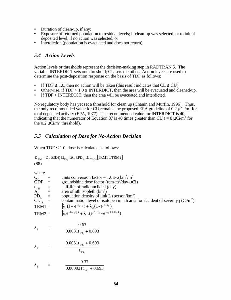
84

• Duration of clean-up, if any;• Exposure of returned population to residual levels; if clean-up was selected, or to initial

deposited level, if no action was selected; or• Interdiction (population is evacuated and does not return).

5.4 Action Levels

Action levels or thresholds represent the decision-making step in RADTRAN 5. Thevariable INTERDICT sets one threshold; CU sets the other. Action levels are used todetermine the post-deposition response on the basis of TDF as follows:

• If TDF ≤ 1.0, then no action will be taken (this result indicates that CL ≤ CU)• Otherwise, if TDF > 1.0 ≤ INTERDICT, then the area will be evacuated and cleaned-up.• If TDF > INTERDICT, then the area will be evacuated and interdicted.

No regulatory body has yet set a threshold for clean up (Chanin and Murfin, 1996). Thus,the only recommended value for CU remains the proposed EPA guideline of 0.2 µCi/m2 fortotal deposited activity (EPA, 1977). The recommended value for INTERDICT is 40,indicating that the numerator of Equation 87 is 40 times greater than CU ( = 8 µCi/m2 forthe 0.2 µCi/m2 threshold).

5.5 Calculation of Dose for No-Action Decision

When TDF ≤ 1.0, dose is calculated as follows:

[ ]TRM2 TRM1CLPDAtGDF Q D ij,n,Ln1/2i7gnd i+⋅⋅⋅⋅⋅=

(88)

whereQ7 = units conversion factor = 1.0E-6 km2/m2

GDF i = groundshine dose factor (rem-m2/day-µCi)t1/2i = half-life of radionuclide i (day)An = area of nth isopleth (km2)PDL = population density of link L (person/km2)CLn,j,i = contamination level of isotope i in nth area for accident of severity j (Ci/m2)TRM1 = )e-(1 )e1( E4E2 T-

3T-

1

TRM2 = )e-(e e 41.83E-T-3

)T(1

4S4S2

λ1 =0.6930.0031t

0.63

i1/2

λ2 =i

i

1/2

1/2

t

0.693 0.0031t

λ3 =693.00.000021t

0.37

i1/2

85

λ4 =i

i

1/2

1/2

t

0.693 0.000021t

TRM 1 in Equation 88 represents the pre-evacuation time period and the exponent TErepresents the elapsed time (days) before evacuation, which the user specifies underkeyword EVACUATION. The second term (TRM2) represents the doses incurred duringthe time in which the area is surveyed (TS exponent) and for a subsequent 50-year period(1.83E+4 days = 50 years) after the evacuated population returns. Doses calculated withEquation 88 are summed over all radionuclides to yield total dose per isopleth area. In theno-action case, there is no difference in the level of deposited concentration because noclean up is performed, and both terms are multiplied by CLi.

5.6 Calculation of Dose for Evacuation and Clean-Up

When 1.0 <TDF≤INTERDICT, the period of time between deposition and the decision toevacuate would precede clean-up efforts and would be the only time inhabitants of thecontaminated area would be exposed to the total amount of radionuclides deposited on theground. The pre-evacuation dose is calculated in the same way as the no-action dose exceptthat TRM2 is multiplied by CU instead of CL, to reflect the lower level of residualradioactivity.

Dgnd = ( ) [ ]CUTRM2CL TRM1 tPDPPSA-AGDF Q i1/2LL1-nni7 i⋅+⋅⋅⋅⋅⋅⋅

(89)whereQ7 = units conversion factor = 1.0E-06 km2/m2

GDF i = groundshine dose factor for isotope i (rem-m2/day-µCi)An = area of nth isopleth (km2)PDL = population density (persons/km2)PPSL = number of packages per shipment on link Lt1/2i = half-life of isotope i (days)TRM1 = see Equation 88TRM2 = see Equation 88

The period of time actually required to carry out a clean-up operation would most likely beprolonged because of regulatory issues, but a relatively short clean-up time may be used forconservatism. The reason a short clean-up period is conservative for public-dose estimationis that a realistic clean-up time (e.g., months or years) permits additional radioactive decay tooccur. As a result, short and moderate half-life radionuclides would decay to quite lowlevels before clean up was completed. This class of radionuclides includes importantgamma producers (e.g., cobalt-60; 1.3 Mev gamma; t1/2 = 5.27 y). The residual radioactivityafter clean up would be depleted in these radionuclides if realistic clean-up times were used. Short clean-up times (e.g., days), on the other hand, would give a proportionalrepresentation of the remaining radionuclide mix, similar to that of the originally depositedmaterial, and would include the short and medium half-life radionuclides. The radionuclidemix will always be depleted in very short half-life isotopes such as I-131 (t1/2 = 8.034 days),regardless of how optimistically the clean-up time is estimated.

Calculation of Dose for Interdiction Decision

86

When TDF > INTERDICT, the deposited concentration of radioactivity in an isopleth areaexceeds the interdiction threshold. The dose is determined by the following.

( ) ij,n,L1-nn2/1i7gnd CLTRM1PDA-A PPS tGDF Q D ⋅⋅⋅⋅⋅⋅⋅=i

(90)

whereQ7 = units conversion factor = 1.0E-06 km2/m2

GDF i = groundshine dose factor for radionuclide i (rem-m2/day-µCi)An = area of nth isopleth (km2)PPS = number of packages per shipment

PDL = population density on link L (persons/km2)t1/2i = half-life of radionuclide i (days)TRM1 = see Equation (88)CLn,j,i = contamination level of radionuclide i in nth area for accident of severity j

In this case, TRM2 is omitted, thereby removing a post-clean-up component of groundshinedose.

Calculation of Total Dose

The decision process for selecting among the triad of options discussed in this section isrepeated for each downwind isopleth. The total dose from groundshine (per accident) iscalculated by summing the results for all isotopes in each isopleth.

Dgnd-Total = ∑=

NAREAS

n 1gndD

(91)

whereDgnd-Total = Total groundshine doseDgnd = Groundshine dose (person-rem) for the ith radionuclide in the nth isoplethin

accident of severity j on link l

5.6.1 Ingestion Dose [optional]

Food supplies may become contaminated by radionuclide deposited in the environment. This pathway is limited to accidents that result in the contamination of agricultural (i.e.,rural) areas. Because the marketing and distribution systems for agricultural products resultin widespread dissemination of contaminated foodstuffs, potentially exposed persons aredistributed throughout the population as a whole and are not restricted to persons living inthe plume deposition “footprint.” The COMIDA computer code (Abbot and Rood, 1993,1994), specifically the second release, COMIDA2, which was developed for use withMACCS2 (Chanin and Young, 1998b) has been used to develop estimates of ingestion dosefor most isotopes in the internal data library.

5.7 Accident Probability and Dose-Risk

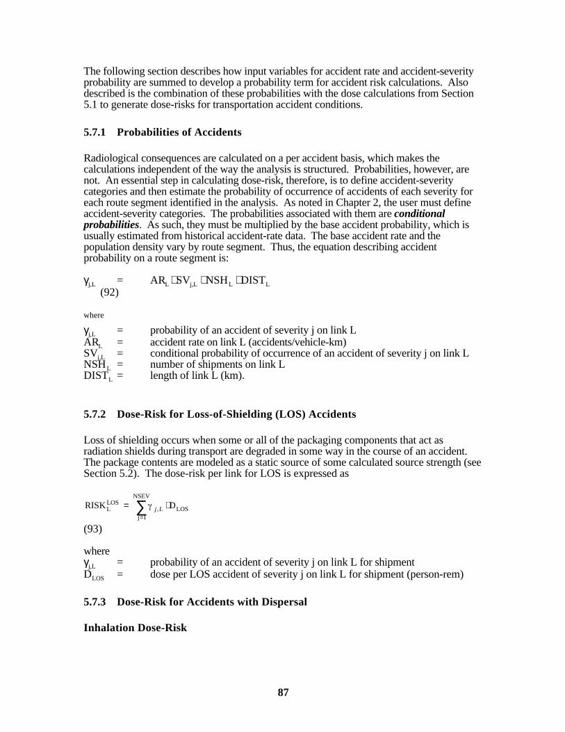
87

The following section describes how input variables for accident rate and accident-severityprobability are summed to develop a probability term for accident risk calculations. Alsodescribed is the combination of these probabilities with the dose calculations from Section5.1 to generate dose-risks for transportation accident conditions.

5.7.1 Probabilities of Accidents

Radiological consequences are calculated on a per accident basis, which makes thecalculations independent of the way the analysis is structured. Probabilities, however, arenot. An essential step in calculating dose-risk, therefore, is to define accident-severitycategories and then estimate the probability of occurrence of accidents of each severity foreach route segment identified in the analysis. As noted in Chapter 2, the user must defineaccident-severity categories. The probabilities associated with them are conditionalprobabilities. As such, they must be multiplied by the base accident probability, which isusually estimated from historical accident-rate data. The base accident rate and thepopulation density vary by route segment. Thus, the equation describing accidentprobability on a route segment is:

γj,L = ARL ⋅ SVj,L ⋅ NSHL ⋅ DISTL (92)

where

γj,L = probability of an accident of severity j on link LARL = accident rate on link L (accidents/vehicle-km)SVj,L = conditional probability of occurrence of an accident of severity j on link LNSHL = number of shipments on link LDISTL = length of link L (km).

5.7.2 Dose-Risk for Loss-of-Shielding (LOS) Accidents

Loss of shielding occurs when some or all of the packaging components that act asradiation shields during transport are degraded in some way in the course of an accident. The package contents are modeled as a static source of some calculated source strength (seeSection 5.2). The dose-risk per link for LOS is expressed as

∑=

⋅=NSEV

1jLOS,

LOSL D RISK Lj

(93)

whereγj,L = probability of an accident of severity j on link L for shipmentDLOS = dose per LOS accident of severity j on link L for shipment (person-rem)

5.7.3 Dose-Risk for Accidents with Dispersal

Inhalation Dose-Risk

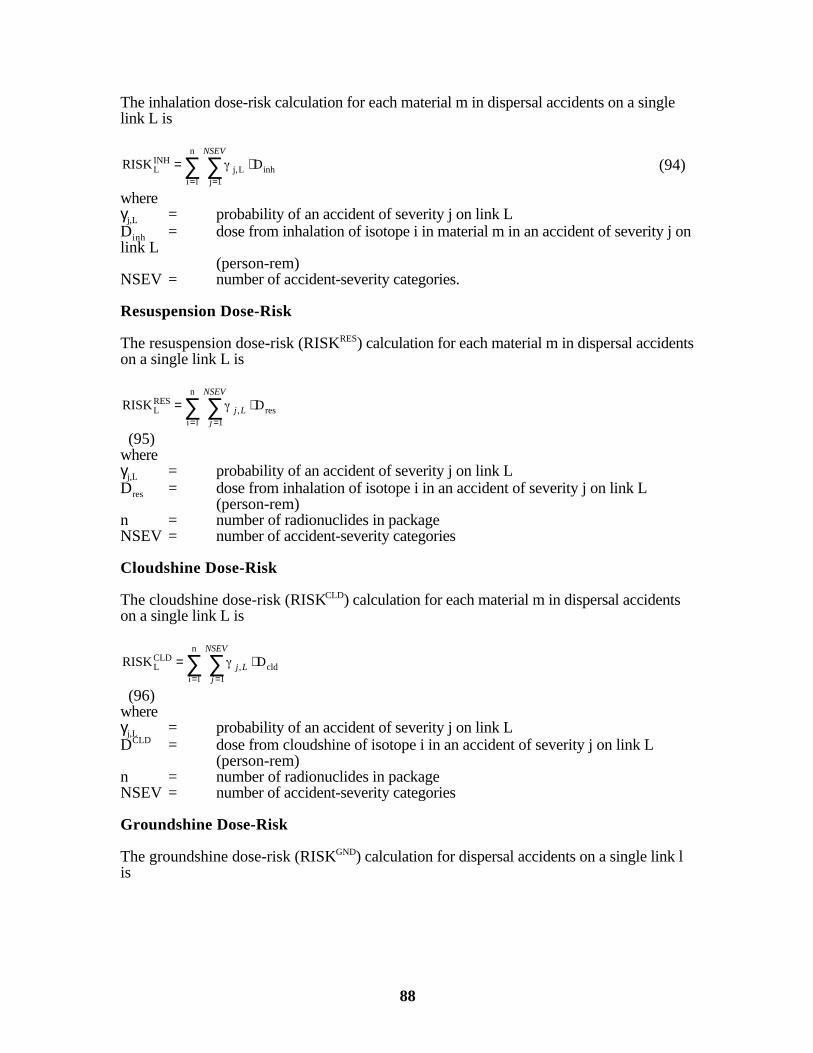
88

The inhalation dose-risk calculation for each material m in dispersal accidents on a singlelink L is

∑ ∑= =

⋅=n

li 1jinhLj,

INHL D RISK

NSEV

(94)

whereγj,L = probability of an accident of severity j on link LDinh = dose from inhalation of isotope i in material m in an accident of severity j onlink L

(person-rem)NSEV = number of accident-severity categories.

Resuspension Dose-Risk

The resuspension dose-risk (RISKRES) calculation for each material m in dispersal accidentson a single link L is

∑ ∑= =

⋅=n

li 1res,

RESL D RISK

NSEV

jLj

(95)whereγj,L = probability of an accident of severity j on link LDres = dose from inhalation of isotope i in an accident of severity j on link L

(person-rem)n = number of radionuclides in packageNSEV = number of accident-severity categories

Cloudshine Dose-Risk

The cloudshine dose-risk (RISKCLD) calculation for each material m in dispersal accidentson a single link L is

∑ ∑= =

⋅=n

li 1cld,

CLDL D RISK

NSEV

jLj

(96)whereγj,L = probability of an accident of severity j on link LDCLD = dose from cloudshine of isotope i in an accident of severity j on link L

(person-rem)n = number of radionuclides in packageNSEV = number of accident-severity categories

Groundshine Dose-Risk

The groundshine dose-risk (RISKGND) calculation for dispersal accidents on a single link lis

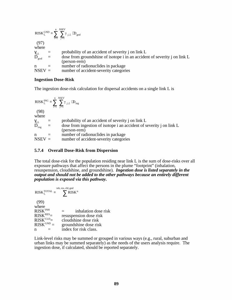
89

∑ ∑= =

⋅=n

li 1gnd,

GNDL D RISK

NSEV

jLj

(97)whereγj,L = probability of an accident of severity j on link LDgnd = dose from groundshine of isotope i in an accident of severity j on link L

(person-rem)n = number of radionuclides in packageNSEV = number of accident-severity categories

Ingestion Dose-Risk

The ingestion dose-risk calculation for dispersal accidents on a single link L is

∑ ∑= =

⋅=n

li 1ing,

INGL D RISK

NSEV

jLj

(98)whereγj,L = probability of an accident of severity j on link LDing = dose from ingestion of isotope i an accident of severity j on link L

(person-rem)n = number of radionuclides in packageNSEV = number of accident-severity categories

5.7.4 Overall Dose-Risk from Dispersion

The total dose-risk for the population residing near link L is the sum of dose-risks over allexposure pathways that affect the persons in the plume “footprint” (inhalation,resuspension, cloudshine, and groundshine). Ingestion dose is listed separately in theoutput and should not be added to the other pathways because an entirely differentpopulation is exposed via this pathway.

∑=gnd cld, res, inh,

nTOTALL RISK RISK

(99)whereRISKINH = inhalation dose riskRISKRES= resuspension dose riskRISKCLD= cloudshine dose riskRISKGND = groundshine dose riskn = index for risk class.

Link-level risks may be summed or grouped in various ways (e.g., rural, suburban andurban links may be summed separately) as the needs of the users analysis require. Theingestion dose, if calculated, should be reported separately.

90

6 Health Effects

6.1 Acute Health EffectsThe nature of health effects that may result from exposure to radiation depends on both thetotal dose and the dose rate. Acute health effects are those that occur when individual doseexceeds some threshold value. Acute effects are also referred to as deterministic effects. Another term that is used is prompt effects since the symptoms appear shortly afterexposure rather than after a long latent period as for most cancers.

A dose sufficient to cause acute health effects must be delivered in a short period of time;varying from a few seconds to a few days depending on the source strength. Such a dosemay be delivered by external radiation and/or by inhalation or ingestion of large amounts ofradioactive material. In the latter case, the lung or intestinal tract, respectively, is the organmost directly irradiated.

Variability in radiation response within a population and variability in the type of medicalcare available mean there is not a single dose threshold for mortality. This has led to the useof LD (lethal dose) metrics. The LD50 , which represents the dose that yields 50% mortalityof an exposed population, is an example. For a single short whole-body exposure toexternal low-LET15 radiation and minimal post-exposure medical treatment, the ReactorSafety Study gave an LD50 of 345 rem (NRC, 1975). More recent data have confirmed thisvalue. The National Council on Radiation Protection (NCRP) gives an LD50/30

16 as a range

of doses with a median of 340 rem whole-body dose for minimal medical care (NCRP,1989). Above this dose, the chance of early mortality increases until it reaches 99% above400 rem with minimal care. The survival rate at this dose level can be almost doubled withintensive medical treatment (e.g., bone marrow transplants), but death is virtually certainabove 1000 rem even with intensive medical care (NRC, 1975; Evans et al., 1985; NCRP,1989). Most thresholds for non-fatal effects, which are referred to as early morbidities, areorgan-based. Some organs, such as the lung, are considerably more radiation resistant thanothers , such as bone marrow. One-year bone marrow doses are calculated and used tomodel the effects of external whole body radiation.

Doses large enough to result in acute effects are so rare in RAM transportation that nonehas yet occurred. In RADTRAN 5 the potential occurrence of early effects is estimated for(a) exposure to external penetrating radiation in LOS scenarios and (b) internal exposurefrom inhaled particulates. The ongoing reassessment of dosimetry for Hiroshima andNagasaki survivors and data from other smaller groups of individuals exposed to highdoses of radiation have resulted in the publication of new models (Evans et al., 1985; NRC,1990; ICRP, 1991) that have replaced the Reactor Safety Study (NRC, 1975). Early effectsvalues in previous releases of RADTRAN were taken from the Reactor Safety Study forminimal care. The early-effects values used in RADTRAN 5 for acute effects are takenfrom Evans et al. (1985) for an intermediate level of care since no values were calculated forminimal care.

15 LET refers to Linear Energy Transfer; low-LET radiations include beta, gamma, and X-rays. Neutrons are the

only types of high-LET external radiation assessed in RADTRAN.

16 LD50/30 is a dose that causes 50% lethality within 30 days.

91

Thresholds for acute effects must be applied at the level of individual dose. In RADTRAN,individual dose estimates by isopleth area or by annular area (for LOS accidents) areexamined to determine whether a threshold has been exceeded. Estimation of acute effectspotentially associated with LOS accidents is discussed in Section 6.1.1. Estimation of acuteeffects potentially associated with inhalation of particulates is discussed in Section 6.1.2. Ifthe RADTRAN stop model was used to calculate LOS dose, then the calculations inSections 6.1.1 and 6.1.2 are not performed automatically and must be performed externallyby the user.

6.1.1 Mathematical Model for Number of Expected Early Fatalities and EarlyMorbidities for Loss-of-Shielding (LOS) Accidents

Early FatalitiesOnce organ doses have been computed as described in Chapter 5 (Equations 74 and 75), theprobability of an early fatality (PEF) is determined. It is the product of a computed dose andthe probability of death as a result of receiving such a dose when receiving an intermediatelevel of medical care (Table 6-1). The expected number of people in each annular area(EXPk), as calculated in Equations 71 through 73, is also a variable. Bone is used torepresent external radiation effects because of the low threshold dose for the organ. Lungdose is used to assess acute mortality from inhalation of particulates following dispersion. The values are derived from Evans et al. (1985). The “old values” from the Reactor SafetyStudy are given in Table 6-2 strictly for comparison purposes.

The expected number of early fatalities (NEF) for each population-density class (rural,suburban, or urban) is then given by:

( )∑=

⋅=NRAD

2k

EFLk,j,k

EFLj, PEXP N

(100)

whereEXPk = expected number of people in kth annular area (from Equations 71 through73)

EFLk,j,P = probability of early fatality for accident of severity j in kth annular area on

link L(computed dose x probability from Table 6-1)

NRAD= number of annular areas (k index).

The summation in Equation 100 starts with k=2 because the innermost annular area ismodeled as an exclusion area, as described in Chapter 5. A severe fire is part of many high-severity accident scenarios. Such a fire usually would force people to leave the 2 or 3innermost annular areas because of the extreme heat. Since it is only within relatively shortradial distances of a shipment that large prompt doses can be incurred as a result of LOS,treating these annuli as being populated in all accident severities leads to early-effectsestimates for LOS that are somewhat conservative. A certain amount of conservatism isderived from the intermediate-care assumption; the number of fatalities can be reduced byintensive medical treatment.

Early Morbidities

92

The approach to estimation of early morbidities is to use a step probability function, PEM,which assumes a value of unity for doses above the threshold and a value of zero for dosesbelow the threshold. The thresholds listed in Table 6-3 represent acute doses above whichsome type of debilitating physiological response is likely (Evans et al., 1985). InRADTRAN 5, the probability of an early morbidity in a LOS accident is determined bycomparison of the calculated individual dose from Equations 74 and 75 in each annular areawith the threshold for external whole-body exposure (bone marrow). The expected numberof early morbidities (NEM-LOS) per accident is then given by:

( )∑=

⋅=NRAD

2k

EMLk,j,k

LOS-EMLj, PEXP N

(101)

Table 6-1. Probabilities of Early Fatality – Marrow and Lung Doses(derived from Evans et al. 1985)

MarrowDose(rem)

FatalityIncidenc

e

MarrowDose(rem)

FatalityIncidenc

e

LungDose(rem)

FatalityIncidenc

e<160 0.00000 570 0.99482 <500 0.00000160 0.00913 580 0.99679 525 0.00759170 0.01234 590 0.99808 550 0.01050180 0.01639 600 0.99889 575 0.01430190 0.02143 610 0.99938 600 0.01922200 0.02761 620 0.99967 625 0.02549210 0.03510 630 0.99983 650 0.03341220 0.04408 640 0.99992 675 0.04329230 0.05475 650 0.99996 700 0.05548240 0.06729 660 0.99998 725 0.07038250 0.08188 6700 0.99999 750 0.08837260 0.09872 >670 1.00000 775 0.10988270 0.11797 800 0.13529280 0.13977 825 0.16498290 0.16425 850 0.19925300 0.19150 875 0.23830310 0.22155 900 0.28218320 0.25438 925 0.33077330 0.28990 950 0.38372340 0.32798 975 0.44042350 0.36838 1000 0.50000360 0.41078 1025 0.56130370 0.45481 1050 0.62293380 0.50000 1075 0.68335390 0.54583 1100 0.74095400 0.59172 1125 0.79420410 0.63706 1150 0.84178420 0.68123 1175 0.88274

93

430 0.72363 1200 0.91656440 0.76371 1225 0.94326450 0.80096 1250 0.96331460 0.83499 1275 0.97755470 0.86552 1300 0.98709480 0.89237 1325 0.99306490 0.91551 1350 0.99653500 0.93502 1375 0.99840510 0.95111 1400 0.99933520 0.96406 1425 0.99974530 0.97423 1450 0.99991540 0.98199 1475 0.99997550 0.98776 1500 0.99999560 0.99192 >1500 1.00000

94

Table 6-2 Comparison of RADTRAN 5 Values withPrevious Fatality Values (abbreviated listing)

Dose(rem)

BoneMarrow

old values

BoneMarrow

new values

Lungold

valuesa

Lungnew values

100,000 1.0 1.0 1.0 1.0 80,000 1.0 1.0 1.0 1.0 70,000 1.0 1.0 1.0 1.0 40,000 1.0 1.0 1.0 1.0 30,000 1.0 1.0 1.0 1.0 25,000 1.0 1.0 1.0 1.0 20,000 1.0 1.0 1.0 1.0 10,000 1.0 1.0 0.60 1.0 8,000 1.0 1.0 0.10 1.0 6,000 1.0 1.0 0.06 1.0 4,000 1.0 1.0 0.03 1.0 3,000 1.0 1.0 0 1.0 2,000 1.0 1.0 0 1.0 1,000 1.0 1.0 0 0.50000 800 0.996 1.0 0 0.13529 700 0.900 1.0 0 0.05548 600 0.400 1.0 0 0.01922 500 0.05 0.999

1.0 if > 6800 0

400 0 0.978 0 0 300 0.770 0 200 0.356 0 150 0 0.083 0 0 100 0 0.012 0 0 <100 0 0 0 0

a. For Lung Type 1 with minimal care; all other values for intermediate level ofcare.

whereEXP = number of people in kth annular areaPEM = probability of early morbidity in accident of severity j in kth annular area onlink L,

whereP = 1 if individual dose is greater than or equal to the threshold, andP = 0 if individual dose is less than the threshold

NRAD = number of annular areas.

Early fatalities are subtracted from early morbidities to prevent double counting of acutehealth effects.

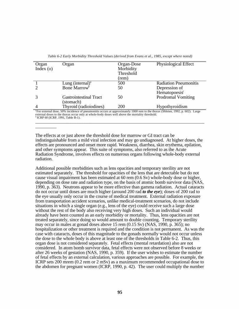
95

Table 6-2 Early Morbidity Threshold Values (derived from Evans et al., 1985, except where noted)

OrganIndex (o)

Organ Organ-DoseMorbidityThreshold(rem)

Physiological Effect

1 Lung (internal)a 500 Radiation Pneumonitis2 Bone Marrowb 50 Depression of

Hematopoesisc

3 Gastrointestinal Tract(stomach)

50 Prodromal Vomiting

4 Thyroid (radioiodines) 200 Hypothyroidisma For external dose, 50% incidence of pneumonitis occurs at approximately 1000 rem to the thorax (Shleien, 1992, p. 602). Largeexternal doses to the thorax occur only at whole-body doses well above the mortality threshold.b ICRP 60 (ICRP, 1991, Table B-1). _________________________________________________________________________________

The effects at or just above the threshold dose for marrow or GI tract can beindistinguishable from a mild viral infection and may go undiagnosed. At higher doses, theeffects are pronounced and onset more rapid. Weakness, diarrhea, skin erythema, epilation,and other symptoms appear. This suite of symptoms, also referred to as the AcuteRadiation Syndrome, involves effects on numerous organs following whole-body externalradiation.

Additional possible morbidities such as lens opacities and temporary sterility are notestimated separately. The threshold for opacities of the lens that are detectable but do notcause visual impairment has been estimated at 60 rem (0.6 Sv) whole-body dose or higher,depending on dose rate and radiation type, on the basis of atomic bomb survivor data (NAS,1990, p. 363). Neutrons appear to be more effective than gamma radiation. Actual cataractsdo not occur until doses are much higher (around 200 rad to the eye); doses of 200 rad tothe eye usually only occur in the course of medical treatment. External radiation exposurefrom transportation accident scenarios, unlike medical-treatment scenarios, do not includesituations in which a single organ (e.g., lens of the eye) could receive such a large dosewithout the rest of the body also receiving very high doses. Such an individual wouldalready have been counted as an early morbidity or mortality. Thus, lens opacities are nottreated separately, since doing so would amount to double counting. Temporary sterilitymay occur in males at gonad doses above 15 rem (0.15 Sv) (NAS, 1990, p. 365); nohospitalization or other treatment is required and the condition is not permanent. As was thecase with cataracts, doses of this magnitude to the gonads normally would not occur unlessthe dose to the whole body is above at least one of the thresholds in Table 6-2. Thus, thisorgan dose is not considered separately. Fetal effects (mental retardation) also are notconsidered. In atom bomb survivor data, fetal effects were not observed before 8 weeks orafter 26 weeks of gestation (NAS, 1990, p. 359). If the user wishes to estimate the numberof fetal effects by an external calculation, various approaches are possible. For example, theICRP sets 200 mrem (0.2 rem or 2 mSv) as a maximum recommended occupational dose tothe abdomen for pregnant women (ICRP, 1990, p. 42). The user could multiply the number

96

of exposed individuals in annuli with total individual doses >200 mrem, if any, (value takendirectly from RADTRAN 5 output) by an appropriate factor17 to generate an estimate.

The primary mechanism for exposure of the thyroid to above-threshold doses is inhalationor ingestion of radioiodine. Hypothyroidism is a non-fatal consequence of radioiodineinhalation or ingestion that results following the death of hormone-producing cells in thethyroid.

6.1.2 Mathematical Model for Number of Acute Health Effects from Inhalation ofDispersed Material

Early FatalitiesThe probability of early fatalities from inhaled radionuclides is calculated in a manneranalogous to the nondispersal case. For each downwind isopleth, An, the lung and bonemarrow organ doses from Equation 76 are compared to the PEF, the probability of earlyfatality (see Table 6-1). The PEF for the lung accounts for dose to the lung itself. The PEF

for bone-marrow accounts for irradiation of the rest of the body by radiation emitted by theinhaled particulates lodged in the lung and for translocation of particles out of the lung andinto other, more radiation-sensitive organs. The expected number of early fatalities is givenby

( )∑∑==

⋅=NAREAS

1n

EFio,n,L,j,n

2

1o

INH-EFLj, PEXP N

(102)where

INH-EFL j,N = number of early fatalities per dispersal accident of severity j on link L

NAREAS= nth isopleth areaEXP = expected number of persons in nth isopleth areaPDn = population density of nth isopleth area (persons/km2)An = area of nth isopleth (km2)EXPn = expected number of people in nth isopleth [PDn⋅(An-An-1)]PEF = probability of early fatality in accident of severity j in nth isopleth for organo

on link L for radionuclide i

Early MorbiditiesEarly morbidity doses are estimated by reference to Equation 76 and by comparison of theorgan doses with the thresholds in Table 6-3. The organs included are the lung, bonemarrow, gastrointestinal tract, and thyroid (radioiodines only). Table 6-3 gives thresholddose values for manifestation of physiological effects. The number of early morbidities isestimated by summing over these organs.

17 E.g., for a pregnancy rate of 3%, the factor would be equal to: chance of being female (~0.5) x chance of female

being pregnant (0.03) x chance of being in week 8 – 26 (~0.53) = 0.008 ≅ 0.01.

97

( )∑ ∑= =

⋅=4

1o

NAREAS

1n

EMon,L,j,n

INH-EMLj, PEXP N

(103)

where

INH-EMLj,N = number of early morbidities per dispersal accident in accident of severity j

NAREAS= nth isopleth areaEXP = expected number of people in nth isopleth area [PDn⋅(An-An-1)]

EMio,n,L,j,P = probability of early morbidity in accident of severity j in nth isopleth area on

link Lfor organ o and radionuclide i, whereP = 1 if individual dose is greater than or equal to the threshold, andP = 0 if individual dose is less than the threshold

PDn = population density in nth isopleth area (persons/km2)An = area of nth isopleth (km2)

6.2 Latent Health Effects

The occurrence of radiogenic cancers and genetic effects is stochastic; that is, theprobability of occurrence increases as dose increases, but the severity of the cancer orgenetic effect does not. RADTRAN 5 uses the linear, no-threshold (LNT) model of thestochastic dose-effect relationship. In the LNT model, the probability of a latent effect isassumed to be a linear function of dose for all doses no matter how small the dose may be. The LNT model is widely regarded as being highly conservative for doses equal to or lessthan background (approximately 300 mrem/year in the United States) (Muckerheide, 1995). The vast majority of doses for incident-free transportation and for most accidents lie in thisrange.

The dose-effect conversions factors used in RADTRAN 5 are taken from BEIR V (NAS,1990) for low doses and low dose-rates; they are consistent with ICRP 60 (ICRP, 1991). They are:1. 5.0E-04 LCF/person-rem for the public2. 4.0E-04 LCF/person-rem for workers.3. 1.0E-04 Genetic Effects/person-rem.

6.2.1 Calculation of Latent Cancer Fatalities and Genetic Effects forNondispersal Accidents

Once integrated population dose is determined, dose-effect conversion factors can beapplied. The expected total dose equivalent and the gonad dose are used to estimateincidence of latent cancers and genetic effects, respectively, giving

LOSLOS-LCF

Lj,i, D LCFC N ⋅= (104)

98

and

gonadLOS

LOS-GELj,i, D GEC N ⋅=

(105)

whereLOS-LCF

Lj,i,N = expected number of latent cancer fatalities per accident of severity jLOS-GE

Lj,i,N = expected number of genetic effects per accident of severity jDLOS = total dose equivalent (person-rem) for accident of severity j

gonadLOSD = organ dose (person-rem) for accident of severity j

LCFC = latent cancer fatalities conversion factor (LCF/person-rem)GEC = genetic effects conversion factor (GE/person-rem).

6.2.2 Calculation of Latent Cancer Fatalities and Genetic Effects for DispersalAccidents

InhalationLatent effects from inhalation are considered for the inhalation dose equivalent and for thegonad dose. The former is given by

inhINH-LCF

ml,j,i, D LCFC N ⋅= (106)

whereNLCF-INH = expected number of latent cancer fatalities from inhalation perdispersal accidentLCFC = dose-effect conversion factor (LCF/person-rem)Dinh = dose equivalent from inhalation (person-rem)

Expected numbers of genetic effects are obtained with the dose-conversion factor forgenetic effects.

gonadinh

INH-GEml,j,i, D GEC N ⋅=

(107)

whereNGE-INH = expected number of genetic effects from inhalation per dispersal accidentGEC = dose-effect conversion factor for genetic effects (LCF/person-rem)

gonadinh

D = gonad organ dose from inhalation (person-rem)

ResuspensionLatent effects from inhalation of resuspended particulates are considered for the inhalationdose equivalent and for the gonad dose. The former is given by

resRES-LCF

ml,j,i, D LCFC N ⋅= (108)

99

whereNLCF-RES = expected number of latent cancer fatalities from resuspension

per dispersal accidentLCFC = dose-effect conversion factor (LCF/person-rem)Dres = dose equivalent from resuspension (person-rem).

Expected numbers of genetic effects are obtained with the dose-conversion factor forgenetic effects.

gonadres

RES-GEml,j,i, D GEC N ⋅=

(109)

whereNGE-RES = expected number of genetic effects from resuspension per dispersal accidentGEC = dose-effect conversion factor for genetic effects (LCF/person-rem)

gonadresD = gonad dose from resuspension (person-rem).

CloudshineLatent effects from exposure to external penetrating radiation during passage of a cloud ofdispersed radioactive material are calculated as follows.

cldCLD-LCF

ml,j,i, D LCFC N ⋅= (110)

and

gonadcld

CLD-GEml,j,i, D GEC N ⋅=

(111)

whereNLCF-CLD = expected number of latent cancer fatalities per accident of severity jNGE-CLD = expected number of genetic effects per accident of severity jDcld = total dose equivalent (person-rem) for accident of severity j from cloudshine

pathwaygonadcldD = gonad organ dose (person-rem) for accident of severity j from cloudshine

pathwayLCFC = latent cancer fatalities conversion factor (LCF/person-rem)GEC = genetic effects conversion factor (GE/person-rem).

GroundshineLatent effects from exposure to external penetrating radiation from deposited radioactivematerial are calculated as follows.

gndGND-LCF

ml,j,i, D LCFC N ⋅= (112)

and

gonadgnd

GND-GEml,j,i, D GEC N ⋅=

(113)

100

whereNLCF-GND= expected number of latent cancer fatalities per accident of severity jNGE-GND= expected number of genetic effects per accident of severity jDgnd = total dose equivalent (person-rem) for accident of severity j fromgroundshine

pathwaygonadgndD = gonad organ dose (person-rem) for accident of severity j from groundshine

pathwayLCFC = latent cancer fatalities conversion factor (LCF/person-rem)GEC = genetic effects conversion factor (GE/person-rem).

IngestionLatent effects from exposure to internal radiation following ingestion of radioactive materialare calculated as follows.

ingING-LCF

ml,j,i, D LCFC N ⋅= (114)

and

gonading

ING-GEml,j,i, D GEC N ⋅=

(115)

whereNLCF-ING = expected number of latent cancer fatalities per accident of severity jNGE-ING = expected number of genetic effects per accident of severity jDing = total dose equivalent (person-rem) for accident of severity j from ingestion

pathwaygonadingD = gonad organ dose (person-rem) for accident of severity j from ingestion

pathwayLCFC = latent cancer fatalities conversion factor (LCF/person-rem)GEC = genetic effects conversion factor (GE/person-rem).

6.3 Total Health Risk from Accidents

Calculation of the expected number of health effects per accident was discussed in Section6.2. For non-dispersal and dispersal accidents alike, the effects are combined with accidentprobabilities to give a total health-effect risk (RISKHE).

ml,j,i,

NSEV

1jlj,

HEml,i, N RISK

(116)

whereNSEV = jth accident-severity categoryγ = probability of occurrence of an accident of severity j on route segment lN = expected number of morbidities, or mortalities, or latent cancer fatalities

101

(LCFs) from all pathways per accident of severity j on route segment linvolving material m

For each route segment, the LCF values calculated by Equation (116) are summed for allmaterials (m index) in the shipment and printed in the RADTRAN 5 output as the health-effects risk for each route segment identified by the analyst. Morbidities and mortalities, ifany, are reported in separate tables.

6.4 Expected Number of Accidents

The formulation for the expected number of accidents is discussed in this section. Thecomputed values are given in a separate table in the RADTRAN 5 output. Calculation ofaccident probability (γ) was described in Chapter 5. The values of γ that are associated witheach specific number of health effects can be combined to give the total expected number ofaccidents for each discrete number of health effects. Because health-effect-inducingaccidents are very infrequent, a Poisson probability density function may be used with theexpected number of accidents as the parameter of the distribution:

B!

eB P(B)

-⋅=

(117)

whereP(B) = probability of exactly B accidentsγ = expected number of accidentsB! = B factorial [=1⋅2⋅3⋅.....⋅(B-1)(B)]. 0! is defined as being equal to 1.

Accidents with zero health effects per accident can be investigated by examining the case ofB=0. To account for the possibility of one accident with exactly zero health effects, theprobability that accidents with zero health effects will occur is computed by use of Equation(117) where B=0 and γ = the probability of accidents with no health effects. Theappropriate value of γ can be obtained by subtracting the expected number of accident withone or more health effects from the total expected number of accidents.

By subtracting the probability of an accident with zero health effects from one (1.0), theprobability of one or more accidents with zero health effects is obtained:

P(1 or more accidents with 0 health effects) = 1 – P(0 health effects) = 1 - eγ (118)

where γ = [probability of no health effects].

In addition, zero health effects can be obtained by having zero accidents. The probabilityassociated with this outcome of transportation is obtained by computing the total expectednumber of accidents of all severities for shipment of material m:

γ = ∑=

⋅⋅NPOP

p

1LmL,L DIST NSH AR

(119)

102

whereARL = accident rate on link L (accident/vehicle-km)NSHL = number of shipments on link L of material mDISTL = length of link L (km)

By applying the Poisson distribution to this value of γ with B=0, the probability of zeroaccidents can be calculated. The results are printed in the output.

6.5 Importance Analysis

RADTRAN 5 performs an importance analysis summary for incident-free transportationfor each link of the route. The importance analysis summary shows the increase ordecrease that every parameter value causes in the outcome of RADTRAN calculations if thevalue is increased by one percent (1%). It measures the relative importance of all theparameters used in a particular input file.

Consider the total incident-free dose, D, given by

a bc21b x,...,x,xd D

(120)

Here, the first summation represents all shipments and the second summation represents alldose subgroups. The importance measure, Ic, is defined as the person-rem change in D,given a one-percent (1%) change in the value of parameter xc. The value of ∆D isapproximated by the product of one percent of each parameter and the first partial derivativeof the dose expression with respect to that parameter. The Importance (I) of the cthparameter is calculated according to

a b c

bc

ccc x

dx

x

D x I

(121)

This can be rewritten as,

ba b bc

cb

ccc d

d x

xd

x

DxI

(122)

or as

ba b c

b

ccc d

ln x d

dln d

x

DxI

(123)

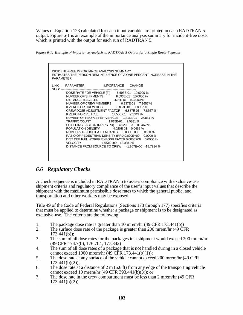
103

Values of Equation 123 calculated for each input variable are printed in each RADTRAN 5output. Figure 6-1 is an example of the importance analysis summary for incident-free dose,which is printed with the output for each run of RADTRAN 5.

Figure 6-1. Example of Importance Analysis in RADTRAN 5 Output for a Single Route-Segment

6.6 Regulatory Checks

A check sequence is included in RADTRAN 5 to assess compliance with exclusive-useshipment criteria and regulatory compliance of the user’s input values that describe theshipment with the maximum permissible dose rates to which the general public, andtransportation and other workers may be exposed.

Title 49 of the Code of Federal Regulations (Sections 173 through 177) specifies criteriathat must be applied to determine whether a package or shipment is to be designated asexclusive-use. The criteria are the following:

1. The package dose rate is greater than 10 mrem/hr (49 CFR 173.441(b))2. The surface dose rate of the package is greater than 200 mrem/hr (49 CFR

173.441(b));3. The sum of all dose rates for the packages in a shipment would exceed 200 mrem/hr

(49 CFR 174.7(b), 176.704, 177.842)4. The sum of all dose rates of a package that is not handled during in a closed vehicle

cannot exceed 1000 mrem/hr (49 CFR 173.441(b)(1));5. The dose rate at any surface of the vehicle cannot exceed 200 mrem/hr (49 CFR

173.441(b)(2));6. The dose rate at a distance of 2 m (6.6 ft) from any edge of the transporting vehicle

cannot exceed 10 mrem/hr (49 CFR 393.441(b)(3)); or7. The dose rate in the crew compartment must be less than 2 mrem/hr (49 CFR

173.441(b)(2))

INCIDENT-FREE IMPORTANCE ANALYSIS SUMMARYESTIMATES THE PERSON-REM INFLUENCE OF A ONE PERCENT INCREASE IN THEPARAMETER

LINK PARAMETER IMPORTANCE CHANGESEG1----------------------------------------------------------------

DOSE RATE FOR VEHICLE (TI) 8.693E-01 10.0000 %NUMBER OF SHIPMENTS 8.693E-01 10.0000 %DISTANCE TRAVELED 8.693E-01 10.0000 %NUMBER OF CREW MEMBERS 6.837E-01 7.8657 %K ZERO FOR CREW DOSE 6.837E-01 7.8657 %CREW DOSE ADJUSTMENT FACTOR 6.837E-01 7.8657 %K ZERO FOR VEHICLE 1.855E-01 2.1343 %NUMBER OF PEOPLE PER VEHICLE 1.815E-01 2.0881 %TRAFFIC COUNT 1.815E-01 2.0881 %SHIELDING FACTOR (RR,RS,RU) 4.020E-03 0.0462 %POPULATION DENSITY 4.020E-03 0.0462 %NUMBER OF FLIGHT ATTENDANTS 0.000E+00 0.0000 %RATIO OF PEDESTRIAN DENSITY (RPD)0.000E+00 0.0000 %DIST DEP RAIL WORKR EXPOSR FACTR 0.000E+00 0.0000 %VELOCITY -1.051E+00 -12.0881 %DISTANCE FROM SOURCE TO CREW -1.367E+00 -15.7314 %

104

The regulatory checks that RADTRAN 5 performs tell the user whether the variables for ashipment of radioactive material that he or she has entered in a RADTRAN 5 input filecomply with Federal regulations for maximum permissible dose rates to population or crew,and with exclusive-use criteria. RADTRAN 5 does not allow the user to perform acomputer run for a shipment that fails to meet these regulations without a printed messagebeing inserted in the output file. Should the user choose to ignore the regulatory checks, amessage stating that the regulatory checks have been disabled will be printed in the output.

6.6.1 Exclusive-Use DesignationAn exclusive-use package is one that must be transported in a vehicle exclusively assignedto that shipment (i.e., shipped without other freight or cargo present in the same vehicle orship hold). There are three criteria, and if any one of them is exceeded, then the packagemust be designated as exclusive-use. 1. Any package with a DRp greater than 10 (mrem/hr);2. Any package with a surface dose rate greater than 200 mrem/hr;3. Any shipment (vehicle) consisting of more than one package in which the summed dose

rate of all packages is greater than 50 (mrem/hr).

A shipment not originally designated exclusive-use by the RADTRAN 5 user will be re-designated as exclusive-sue (i.e., the exclusive-use flag in the input file may be reset to true),if any of the test results are true. That is, if• DRp > 10

• dimension package sticcharacteri theis d where200, 0.5d

0.5d 1DR

p

p

p

ee

ep >

+

• shipment. in the i typeof packages ofnumber theis PPS where50, PPSDR i

n i

1 ip i

>⋅∑=

=

The second formula extrapolates the package dose rate to the surface on the basis of theradial distance from the line-source representation of the package by use of thecharacteristic package dimension and the line-source model.

If one of these regulatory criteria is exceeded, execution of RADTRAN 5 is not stopped, butan informational message describing the exceedance is printed in the output. This allowsthe user to analyze shipments that may exceed the criteria. Some radiopharmaceuticalshipments, for example, may take place under a waiver of the third rule. If all three tests aresatisfied, then the shipment meets the nonexclusive-use requirements, the calculationproceeds, and no informational message is printed in the output.

Satisfying these tests does not mean that the shipment cannot be exclusive-use, only that itis not required to be. However, if a particular shipment is designated exclusive-use by theanalyst, then it must comply with exclusive-use regulations, which involve additionalregulatory checks described below.

By regulation, the dose rate at any point on the outer surface of the exclusive-use vehiclecannot exceed 200 mrem/hr [10 CFR 71.47 and 49 CFR 173.441(b)]. In addition to thepackage-surface check described above, RADTRAN 5 performs a check of the dose rate atthe outer surface of the vehicle (under the assumption that there is no intervening spacebetween the vehicle surface and package surfaces). The vehicle is treated as a line source atdistances closer than 1 m. The surface dose rate is given by

105

v

v

e

evsurface 0.5d

0.5d 1 DR DR

+=

(124)whereDRsurface = dose rate a vehicle surface (mrem/hr)DRv = vehicle dose rate at 1 m from surface (mrem/hr)

ved = effective dimension of shipment vehicle (m)

In this case, if the regulatory limit of 200 mrem/hr for vehicle surface dose rate is exceeded,then DRv is reset to the result of the following expression for all subsequent calculations

+

=v

v

e

ev 0.5d 1

0.5d200 DR

(125)

The following message is printed in the output to inform the user:FOR [vehicle label] THE SURFACE DOSE RATE COULD EXCEED 200MREM/HR.THE VEHICLE DOSE RATE HAS BEEN RESET TO EQUAL [y]where y = result of Equation 125.

Once the surface dose rate check is satisfied, then the dose rate in the crew compartment(DR) is examined to determine whether the calculated value is less than or equal to theregulatory limit of 2 mrem/hr by evaluating the following expression.

⋅+

⋅⋅⋅=

2end

rN,v2end

rG,vvvend 0,crew

r

TRFN

r

TR FGCSF DR k DR

(126)

whereDRcrew = dose rate in the crew compartment (mrem/hr)k0,end = point-source crew-view shape factor (m)DRv = vehicle dose rate (mrem/hr)CSFv = crew shielding factor for vehicle vFGv = fraction of vehicle dose rate from gamma radiationFNv = fraction of vehicle dose rate from neutron radiationTRG,r = gamma dose-distance relationship at distance rTRN,r = neutron dose-distance relationship at distance rrend = distance from source to crew (m)

The crew-view shape factor (k0,end) is determined by use of Equation to a de derived from thecharacteristic dimension of the package surface closest to the crew compartment. For spent-fuel truck shipments, for example, this dimension would usually be the cask diameter. If thedose rate is acceptable, then the actual value is used for calculating dose to crewmembers. Ifthe dose rate is calculated to be greater than 2 mrem/hr, then the value is reset to 2 mrem/hrfor the calculation of crew dose because measures (e.g., added shielding) must have beentaken to ensure regulatory compliance before transportation is permitted. The followingmessage is printed in the output to inform the user.

106

FOR THE SHIPMENT OF [vehicle label] THE DOSE RATE IN THE CREWCOMPARTMENT COULD EXCEED 2 MREM/HR. THE DOSE RATE HAS BEENRESET FROM [x] TO 2 FOR CREW DOSE CALCULATIONSwhere x = result of Equation 21.

If this test is satisfied, then RADTRAN 5 examines the dose rate at 2 m from the edge ofthe vehicle. Packages are modeled as being located at the edge of the vehicle, and the loadedvehicle is assigned a line source configuration. The expression for this dose rate is

,0.5d 2

0.5d 1 DR m) (2DR

v

v

e

evv

++

⋅=

(127)

whereDRv(2 m)= total dose rate at 2 m from the vehicle surface (mrem/hr)DRv = total dose rate at 1 m from the vehicle surface (mrem/hr)

ved = effective dimension of shipment vehicle (m)

If the vehicle dose rate at 2 meters exceeds 10 mrem/hr, then DR is set equal to

−+

v

v

e

e

0.5d1

d5.02 10 for the calculation of dose to persons along the transport link, dose to

persons sharing the transport link, and dose while stopped. This is done in anticipation ofregulatory compliance, and the following informational message is printed:FOR THE SHIPMENT OF [vehicle label], THE DOSE RATE A 2 METERS COULDEXCEED 10 MREM/HR. THE VEHICLE DOSE RATE HAS BEEN RESET TOEQUAL [z].

where z =

−+

v

v

e

e

0.5d1

d5.02 10

Otherwise, DRv is used directly. In addition, several quantitative criteria must be satisfied. These criteria are:A. For all modes except air, if a shipment is designated as exclusive-use but is not

required to be, then the following message is printed:THE SHIPMENT BY [vehicle label] IS DESIGNATED AS EXCLUSIVE USE BUTIS NOT REQUIRED TO BE SO DESIGNATED BY REGULATIONS.

B. If a shipment is designated as exclusive-use and is by air mode, then the followingmessage is printed:

!!!! WARNING !!!! 49 CFR 173 DOES NOT PERMIT EXCLUSIVE USE AIRSHIPMENTS, COMPUTATIONS PROCEED...

C. Conversely, if a shipment has not been designated as exclusive-use, but is requiredto be, then the following message is printed in the output:

[vehicle label] HAS BEEN DESIGNATED AS EXCLUSIVE USE.

107

7 Special Topics

7.1 RADTRAN 5 ValidationValidation is the process of ensuring that a model embodied in a code is an

acceptable representation of the process it is intended to replicate.

7.1.1 Source Representation in Incident-Free Dose CalculationsThe incident-free dose calculations in RADTRAN 5 are based on idealized models of RAMpackages and conveyances. The models do not directly account for secondary factors suchas reflection and shielding by the conveyance itself and, in some cases, intervening objects. The models conservatively estimate the influence of build-up and attenuation. Thus, theyare somewhat conservative in all situations. The degree of conservatism has not been fullyquantified, but preliminary empirical results indicate that RADTRAN yields values for off-link dose that are a factor of eight to ten higher than measured values (McFadden, Boles,and Steinman, 1999). This is consistent with earlier studies with the INTERTRAN code(based on RADTRAN II) (Permattei et al., 1985; DeMarco et al., 1983). The latter authorsfound that the INTERTRAN/RADTRAN II predictions were larger than measured dosesfor several classes of incident-free dose. In fact, Permattei et al. had difficulty detecting ameasurable dose at locations immediately adjacent to the transport route for actual spent fuelshipments in Italy.

7.1.2 Health Effects Conversion FactorsThe validity of the calculations that RADTRAN performs also depends on the health-physics community’s understanding of radiological health effects causation and on theaccuracy and completeness of user-supplied data. The health-effects model from the“Reactor Safety Study” (NRC, 1975), which is obsolete, was formerly hard-coded intoRADTRAN. It is absent from RADTRAN 5; and the equations have been modified topermit currently accepted dose-effect conversion factors to be used as direct multipliers ofthe dose-consequence calculations. The factors now used calculate LCFs for a linear, no-threshold (LNT) model, modified for low-dose, low-dose-rate situations. The factors are5E-04 LCFs per person-rem for the general public and 4E-10 LCFs per person-rem forworkers (ICRP 60, 1990; NRC, 1989)). A recently empanelled BEIR (Biological Effects ofIonizing Radiation) committee of the National Research Council will be criticallyreexamining the LNT model. RADTRAN 5 may require modification following thepublication of their report.

7.1.3 Package Behavior and Accident ProbabilitiesRADTRAN 5 does not contain a specific model of package behavior for any given packagetype. The user must define these values for the problem at hand, but recommended inputvalues, based on package test data, event trees, DOT data, etc. are available for manyproblems and are included in the sample files at the TRANSNET Internet site. All suchvalues are subject to ongoing re-evaluation. For example, a recent major reassessment ofmaritime transportation (Sprung et al., 1998) supercedes earlier analyses (e.g., DOE, 1986);the newer values yield somewhat lower risk estimates than the older work.

7.2 Verification and Software Quality Assurance

108

Verification is the process of ensuring that the equations formulated by a code’sdevelopers are faithfully executed in the program. The method of verification used isdescribed in Kanipe and Neuhauser (1995) and in the RADTRAN 5 Software QualityAssurance Plan (SQAP) (Kanipe and Neuhauser, 2000). The RADTRAN 5 SQAP followsANSI guidance and standard reporting outlines. As part of the QA plan, all code revisionsare logged; this log is made available on the Internet at the TRANSNET site.

7.3 Non-Radiological Risk - Fatality Risk

Risk of fatality associated with transportation accidents but having non-radiological causes(e.g., physical trauma, fire) is calculated by RADTRAN 5 and printed in the output for eachroute-segment in the analysis.The expected number of non-radiological fatalities (FATAL) is calculated by

LLuor s, r,L NSH DIST NONRAD 2 FATAL ⋅⋅⋅= (124)

whereNONRAD = rural, suburban, or urban nonradiological fatality rate (fatalities/km)DIST = length of Lth route segment (km)NSH = number of shipments on Lth route segment

The factor of two is included to account for return trips when the vehicle is traveling withoutradioactive material cargo. The appropriate value of NONRAD is determined by the user’sdesignation of each route segment as being rural, suburban, or urban in nature.

7.4 RADDOG Input File Generator

RADDOG is a PC-compatible code written in C+ and developed for use with RADTRAN. It allows the user to build a RADTRAN input file ‘from scratch’ or by editing a previousfile. RADDOG applications are discussed extensively in the RADTRAN 5 User Guide(Neuhauser and Kanipe, 2000)

7.5 Geographical Information System (GIS) Data

A Geographical Information System or GIS can be an important source of data for aRADTRAN input file (Ganter and Neuhauser, 1995). A GIS is particularly well suited toroute-segment definition and to development of data on population density and populationsubgroups (e.g., environmental justice). The underlying data generated by a GIS can beconverted into one or more spreadsheets (e.g., with Microsoft Excel®). The relevant datacan then be extracted and placed in a RADTRAN input file. A GIS has been developed atSandia National Laboratories that currently uses 1990 census-block data (with updates) toestimate population densities within specified population bandwidths around atransportation link and under a plume footprint anywhere in the United States. Thedevelopment of data with the Sandia GIS has been automated (Mills and Neuhauser,1999c).

109

It is anticipated that data and graphics developed from the Sandia GIS will be made availableon the TRANSNET site along with the input files routinely published on the site for allanalyses performed by Sandia National Laboratories. The actual GIS cannot be madeinteractive, of course, because the very large graphics files make transmission over phonelines virtually impossible. Many states, counties and cities have developed similar GISs fortheir own areas. These are powerful sources of high-resolution data and users areencouraged to seek them out. Recent applications of the Sandia GIS include:• examination of urban-area avoidance in truck routing (Mills and Neuhauser, 1998);• diurnal variation in off-link population density (Mills and Neuhauser, 1999a);• comparison of methods of estimating population under a dispersion plume (Mills and

Neuhauser, 1999b); and• development of environmental-justice methods for transportation (Mills and Neuhauser,

2000).

7.6 Latin Hypercube Sampling (LHS) Interface

Latin Hypercube Sampling (LHS) is a method of Monte Carlo analysis that relies onstructured sampling from one or more parameter probability distributions (e.g., emergency-response-time distribution). With LHS, a relatively small number of samples (usually 50 to100) can be used to generate a meaningful CCDF (Complementary Cumulative DensityFunction). CCDFs are used to graphically illustrate the results of a probabilistic riskanalysis. LHS is also ideally suited to sensitivity analysis applications, as was demonstratedwith RADTRAN 4 (Mills, Neuhauser, and Kanipe, 1995). A semi-automated interface withthe Sandia National Laboratories’ LHS code (Wyss and Jorgensen, 1998) has beendeveloped for RADTRAN 5. Its use is discussed in detail in the RADTRAN 5 User Guide(Neuhauser and Kanipe, 1999).

7.7 Population Residence Time

Demographic data from the U.S. Bureau of the Census indicate that approximately 80% ofthe U.S. population relocate every three years (Israeli and Nelson, 1992). One ramificationof this phenomenon is that for multi-year shipping campaigns (e.g., shipments to a spent-fuel repository) potentially exposed populations living near the transportation route wouldnot consist in subsequent years entirely of the same people as those who resided there in thefirst year. The Census Bureau data were used to develop an algorithm to account for this(Smith, Neuhauser, and Kanipe, 1996). The RADTRAN 5 output contains a section thatgives the estimated total number of persons residing within a designated bandwidth duringthe user-specified number of years over which the shipments will occur (specified bykeyword CAMPAIGN). One limitation of the calculation is that it does not explicitlyaccount for situations in which occupancy is less than 100%, although a “background”level of vacancies is part of the original demographic data. Persons who move in and out ofan area are modeled as replacing each other, so the same size of population is modeled asbeing exposed for each trip. Thus, this calculation has no effect on the off-link populationdose calculated by RADTRAN 5, only on the size of the affected population.

èAlthough it is tempting to divide the cumulative off-link population dose by the totalpopulation to obtain an average individual incident-free dose, the resulting value ismeaningless. The decrease in radiation intensity with the square of distance from the

110

source and the wide variation in residence time at the individual level (for long shippingcampaigns) jointly dictate that such an “average dose” would tell one little about theradiological status of the potentially exposed population. The individual dose subroutine isrecommended instead for calculation of doses to receptors at various distances from and/orwith varied frequencies of exposure to multiple shipments.

Another aspect of demographic change is increases/decreases in population density overtime (most commonly seen as an increase in areas of suburban density). This phenomenonis not explicitly modeled in RADTRAN 5. However, projections of growth may be used tocompare hypothetical future route-related risk predictions with present (baseline) values inexactly the same manner as that used to compare two distinct routes.

7.8 Environmental Justice

Environmental justice in transportation must be addressed in environmental impactstatements (EISs) and environmental assessments (EAs). Bullard and Johnson (1997)discuss examples of environmental justice issues in transportation. RADTRAN 5 may usedin conjunction with a GIS (see Section 7.4) to objectively and quantitatively analyzepotential differences in impacts on population subgroups that may occur as a result of arouting decision. Two types of analysis may be performed. The first type involvescomparisons of two or more routes. Either the relative frequency of occurrence or the actualresident population sizes of racial, economic, or other minority groups may be compared. For these comparisons to be meaningful, the routes should be broken up into segments thatreflect the socio-economic zones through which the route passes, and the results for eachsegment should be calculated separately. The second type of analysis involves comparisonsof the minority make-up of populations residing within various distances (bandwidths) of asingle transportation link. This can be used, for example, to determine whether minorityrepresentation near a transportation corridor is higher than in other areas of the same city,county, etc. Examples of both types of analyses are examined in Mills and Neuhauser(2000).

111

8 Literature Cited

Abbot, M. L. and A. S. Rood, 1993, “COMIDA: A Radionuclide Food Chain Model forAcute Fallout Deposition,” EGG-GEO-10367, Idaho National Engineering Laboratory,Idaho Falls, ID.

Abbot, M. L. and A. S. Rood, 1994, “COMIDA: A Radionuclide Food Chain Model forAcute Fallout Deposition,” Health Physics 66(1), p. 17-29.

AEC (U.S. Atomic Energy Commission), 1972, “Environmental Survey of Transportationof Radioactive Materials to and from Nuclear Power Plants,” WASH-1238, AEC,Washington, DC.

Barker, R., D. Hopkins, A. Tse, 1974, “Radiation Dose to Population (Crew andPassengers) Resulting from the Transportation of Radioactive Material by PassengerAircraft in the United States,” IAEA-SM-184/15, International Atomic Energy Agency,Vienna, Austria.

Beres, D. (Editor), 1990, "The Clean Air Act Assessment Package - 1988 (CAP-88) A Doseand Risk Assessment Methodology for Radionuclide Emissions to Air", Volume 1, User'sManual, U.S. EPA (U.S. Environmental Protection Agency), Washington, DC.

Brogan, J. D., J. W. Cashwell, and K. S. Neuhauser, 1989, “Demographic andTransportation Parameters in RADTRAN,” 9th International Symposium on the Packagingand Transportation of Radioactive Materials (PATRAM’89), Washington, DC, p. 1611-1617.

Boughton, B. S. and J. M. DeLaurentis, 1992, “Description and Validation of ERAD: AnAtmospheric Dispersion Model for High Explosive Detonations,” SAND92-2069, SandiaNational Laboratories, Albuquerque, NM.

Bullard, R. D. and G. S. Johnson (Eds.), 1997, Just Transportation, New SocietyPublishers, Gabriola Island, BC, Canada.

Chanin, D. and M. L. Young, 1998a, "Code Manual for MACCS2, User's Guide,"NUREG/CR-6613, Vol. 1, (SAND97-0594), Nuclear Regulatory Commission,Washington, DC.

Chanin, D. and M. L. Young, 1998b, “Code Manual for MACCS2: Preprocessor CodesCOMIDA2, FGRDCF, IDCF2,” NUREG/CR-6613, Vol. 2, (SAND97-0594), NuclearRegulatory Commission, Washington, DC.

Chapman, C. R., 1998, “Statement on the Threat of Impact of Near-Earth Asteroids by Dr.Clark R. Chapman, Southwest Research Institute,” U.S. Congressional Hearings on Near-Earth Objects and Planetary Defense, May 21, 1998, Washington, DC.

Cohrssen, J. J. and V. T. Covello, 1989, Risk Analysis: A Guide to Principles andMethods for Analyzing Health and Environmental Risks, Chapter 2, U. S. Council onEnvironmental Quality, Washington DC.

112

DeMarco, I., S. Mancioppi, S. Permattei, and G. Scarpa, 1983, “Evaluation of Doses toWorkers and General Public from the Carriage of Radiopharmaceuticals – An Applicationof the INTERTRAN Code,” 7th International Symposium on Packaging and Transportationof Radioactive Materials (PATRAM ’83), New Orleans, LA, p. 173-183.

DOE, 1988, "External Dose-Rate Conversion Factors for Calculation of Dose to thePublic," DOE/EH-0070, U.S. Department of Energy, Washington, D.C.

DOE, 1986, “Environmental Assessment on Shipment of Taiwanese Research Reactorspent Nuclear Fuel." DOE/EA-0321, U.S. Department of Energy, Washington, DC.

Eckerman, K.F., A.B. Wolbarst, and A.C.B. Richardson, 1988, "Limiting Values ofRadionuclide Intake and Air Concentration and Dose Conversion Factors for Inhalation,Submersion, and Ingestion," Federal Guidance Report No. 11, EPA-520/1-88-020, U.S.Environmental Protection Agency, Washington, D.C.

Eckerman, K.F. and J.C. Ryman, 1993, "External Exposure to Radionuclides in Air, Water,and Soil," Federal Guidance Report No. 12, EPA-402-R-93-081, U.S. EnvironmentalProtection Agency, Washington, D.C.

Eicholz, G.G., 1983, “Source terms for nuclear facilities and medical and industrial sites.''in Radiological Assessment, J. E. Till and H. R. Meyer (eds.), NUREG/CR-3332, ORNL-5968. U.S. Nuclear Regulatory Commission, Washington, D. C

Engelmann, R.J., 1990, “Effectiveness of Sheltering in Buildings and Vehicles forPlutonium,” DOE/EH-0159T, U.S. Department of Energy, Washington, D.C.

Ensminger, D.A., C.M. Koplik, and J.Y. Nalbandian, 1987, “User’s Guide to MARINRADIV: Model for Assessing the Consequences of Release of Radioactive Material into theOceans,” SAND87-7067, Sandia National Laboratories, Albuquerque, NM

Environmental Protection Agency (EPA), 1977, “Summary Report: Proposed Guidance onDose Limits for Persons Exposed to Transuranium Elements in the General Environment,”EPA 520/4-77-016, Washington, DC.

Evans, J. S., D. W. Moeller and D. W. Cooper, 1985, “Health Effects Model for NuclearPower Plant Accident Consequence Analysis,” NUREG/CR-4214 (SAND85-7185), USNuclear Regulatory Commission, Washington, DC.

Finley, N. C., et al., 1980, “Transportation of Radionuclides in Urban Environs – DraftEnvironmental Assessment,” NUREG-CR/0743 (SAND79-0369), Nuclear RegulatoryCommission, Washington, DC.

Fischer, L. et al., 1987, "Shipping Container Response to Severe Highway and RailwayAccident Conditions." Volume 1 - Main Report, NUREG/CR-4829, UCID-20733, USNuclear Regulatory Commission, Washington, DC

Ganter, J. H. and K. S. Neuhauser, 1995, “Development of a Geographic InformationSystem (GIS) Application for RADTRAN Input Data Extraction and Display,” 11th

International Conference on the Packaging and Transportation of Radioactive Materials(PATRAM’95), Las Vegas, NV.

Glasstone, S. and A. Sesonske, 1991, “Nuclear Reactor Engineering,” 3rd Edition, KriegerPublishing Co., Malabar, FL.

113

Griego, N. R., J. D. Smith, and K. S. Neuhauser, 1996, “Investigation of RADTRAN StopModel Input Parameters for Truck Stops,” Waste Management ’96, Tucson, AZ.

ICRP (International Commission on Radiological Protection), 1991, “1990Recommendations of the International Commission on Radiological Protection,” ICRPPublication 60, published as Volume 21(1 –3) of the Annals of the ICRP, Pergamon Press,Oxford, England, UK

ICRP (International Commission on Radiological Protection), 1994, “Dose Coefficients forIntakes of Radionuclides by Workers,” ICRP Publication 68, published as Volume 24(4)of the Annals of the ICRP, Pergamon Press, Oxford, England, UK

Israeli, M. and C. B. Nelson, 1992, “Distribution and Expected Time of Residence for U.S.Households,” Risk Analysis 12(1).

Helton, J. C., 1991, “Performance Assessment Overview,” in “Preliminary Comparisonwith 40 CFR Part 191 Subpart A for the Waste Isolation Pilot Plant, December 1991,”SAND91-0893, Sandia National Laboratories, Albuquerque, NM.

Jefferson, T. H., 1982, “MATHDOC AND SLATEC – A USER’S GUIDE,” SAND82-8767, Sandia National Laboratories, Albuquerque, NM.

Kanipe, F. L., 2000, “RADTRAN 5 Programmer’s Manual,” (in press)

Kanipe, F. L. and K. S. Neuhauser, 1995, “Verification of RADTRAN,” 11th InternationalSymposium on Packaging and Transportation of Radioactive Materials (PATRAM ’95), p.713, Las Vegas, NV

Kanipe and Neuhauser, 2000, “RADTRAN 5 Software Quality Assurance Plan,” (inpreparation)

Kinsey, R. and B. A. Magurno, Eds., 1983, “Data Formats and Procedures for theEvaluated Nuclear Data File, ENDF/B-V,” BNL-NCS-50496 (ENDF-102), BrookhavenNational Laboratory, Brookhaven, NY.

Luna, R. E. and H. W. Church, 1969, “DIFOUT: A Model for Computation of AerosolTransport and Diffusion in the Atmosphere,” SC-RR-68-555, Sandia NationalLaboratories, Albuquerque, NM 1969.

Luna, R. E. and H. W. Church, 1972, “A Comparison of Turbulence Intensity and StabilityRatio Measurements to Pasquill Stability Classes,” Journal of Applied Meteorology 11(4),p. 663-669.

Luna, R. E. and H. W. Church, 1974, “Estimation of Long-Term Concentrations Using a“Universal” Wind Speed Distribution,” Journal of Applied Meteorology 15(8), p. 910-916.

McFadden, J. G., Boles, and J. L., Steinman, R. L., 1999, “Final Progress Report forRADTRAN Benchmarking FY99,” Waste Management Technical Services, ENG-RPT-026, Rev. 0, Richland, WA.

114

McFarlane, R. E., D. W. Muir, and R. M. Boicourt, 1982, “The NJOY Nuclear DataProcessing System, Vol. I: User’s Manual,” LA-9303-M, Los Alamos NationalLaboratory, Los Alamos, NM

Madsen, M. M. and E. L. Wilmot, 1983, “Truck Transportation of Radioactive Materials,”7th International Symposium on Packaging and Transportation of Radioactive Materials(PATRAM ’83), New Orleans, LA

Madsen, M. M., E. L. Wilmot and J. M. Taylor, 1986, “RADTRAN II User Guide,”SAND82-2681, Sandia National Laboratories, Albuquerque, NM.

Mills, G. S. and K. S. Neuhauser, 1998, “Urban Risks of Truck Transport of RadioactiveMaterial,” Risk Analysis 18(6), 781-785.

Mills, G. S. and K. S. Neuhauser, 1999a, “Comparison of Daytime and Night-TimePopulations Adjacent to Interstate Highways in Metropolitan Areas,” RAMTRANS(International Journal of Radioactive Materials Transport) 10(2), p.101-104,Nuclear Technology Publishing, UK

Mills, G. S. and K. S. Neuhauser, 1999b, “Statistical Evaluation of Population Data forCalculation of Radioactive Material Transport Accident Risks,” Risk Analysis 19(4), 613-619.

Mills, G. S. and K. S. Neuhauser, 1999c, Automation of GIS-Based Population Data-Collection for Transportation Risk Analysis,” SAND99-2676, Sandia NationalLaboratories, Albuquerque, NM

Mills, G. S. and K. S. Neuhauser, 2000, “Quantitative Methods for Environmental JusticeAssessment of Transportation,” Risk Analysis (accepted for publication in early 2000)

Mills, G. S., K. S. Neuhauser, and F. L. Kanipe, 1995, “RADTRAN 4 Truck Accident-Risk Sensitivity Analysis,” Waste Management ’95, Tucson, AZ.

Mills, G.S., K. S. Neuhauser, and J. D. Smith, 1995, “Study of Evacuation Times Based onGeneral Accident History,” 11th International Conference of the Packaging andTransportation of Radioactive Materials (PATRAM ’95), Las Vegas, NV, p. 719-723.

Muckerheide, J., 1990, “The Health Effects of Low-Level Radiation: Science, data andcorrective action." Nuclear News 38(11), publication of the American Nuclear Society.

Moore, R. E., C. F. Baes III, L. M. McDowell-Boyer, A. P. Watson, F. O. Hoffman, J. E.Pleasant, and C. W. Miller, 1979, "AIRDOS-EPA: A Computerized Methodology forEstimating Environmental Concentrations and Dose to Man from Airborne Releases ofRadionuclides," ORNL-5532, Oak Ridge National Laboratory, Oak Ridge, TN.

NAS/NRC (National Academy of Science/National Research Council), 1990, “HealthEffects of Exposure to Low Levels of Ionizing Radiation,” BEIR V, Committee on theBiological Effects of Ionizing Radiation, NAS/NRC, National Academy Press, Washington,DC.

Neuhauser, K. S., 1992, “Application of RADTRAN to Estimation of Dose to Persons inEnclosed Spaces,” 10th International Symposium on the Packaging and Transportation ofRadioactive Materials, PATRAM ’92, Yokohama City, Japan.

115

Neuhauser, K. S. and F. L. Kanipe, 1992, “RADTRAN 4: User Guide,” SAND89-2370,Sandia National Laboratories, Albuquerque, NM.

Neuhauser, K. S. and F. L. Kanipe, 2000, “RADTRAN 5 User Guide,” SAND2000-1257,Sandia National Laboratories, Albuquerque, NM.

Neuhauser, K. S. and R. F. Weiner, 1992, “Intermodal Transfer of Spent Fuel,” 10th

International Symposium on the Packaging and Transportation of Radioactive Materials,PATRAM ’92, Yokohama City, Japan.

NRC, 1975, “Reactor Safety Study,” WASH-1400, U.S. Nuclear Regulatory Commission,Washington, DC.

NRC, 1977, “Final Environmental Statement on the Transportation of Radioactive Materialby Air and Other Modes,” NUREG-1070, U.S. Nuclear Regulatory Commission,Washington, DC

O’Dell, R. D., F. W. Brinkley, and D. R. Marr, 1982, “User’s Manual for ONEDANT: ACode Package for One-Dimensional, Diffusion-Accelerated, Neutral-Particle Transport,”LA-9184-M, Los Alamos National Laboratory, Los Alamos, NM.

Ostmeyer, 1986, "A Revised Rail-Stop Exposure Model for Incident-Free Transport ofNuclear Waste." SAND85-2149, TTC-0606, February 1986, Sandia National Laboratories,Albuquerque, NM.

Parks, B. S., 1992, “User’s Guide for CAP88-PC Version 1, EPA-402-B-92-001, U.S.Environmental Protection Agency, Washington, DC.

Parks, C. V., B. L. Broadhead, O. W. Hermann, J. S. Tang, S. N. Cramer, J. C. Gauthey, B.L. Kirk, and R. W. Roussin, 1988, “Assessment of Shielding Analysis Methods, Codes,and Data for Spent Fuel Transport/Storage Applications,” ORNL/CSD/TM-246, OakRidge National Laboratories, Oak Ridge, TN.

Pasquill, F., 1961, “Estimation of the Dispersion of Windborne Material,” TheMeteorology Magazine 90, p. 33-49.

Permattei, S., S. Mancioppi, and G. Scarpa, 1985, “Assessment of Individual and CollectiveDoses to Transport Workers and Population from Transport of Irradiated Fuels” in“Chairman’s Report, Technical Committee on the Assessment of the Radiological Impactfrom the Transport of Radioactive Materials,” TC-556, Addendum, International AtomicEnergy Agency, Vienna, Austria.

Petersen, W. B. and L. Lavdas, 1986, “INPUFF2.0: A Multiple Source Gaussian PuffDispersion Algorithm,” EPA-600/8-86/024, U.S. Environmental Protection Agency,Research Triangle Park, NC.Shleien, B. (Ed.), 1992, The Health Physics and Radiological Health Handbook, RevisedEdition, Scinta, Inc., Silver Spring, MD

Smith, J. D., K. S. Neuhauser and F. L. Kanipe, 1996, “Expected Residence Time Model,”Waste Management ’96, Tucson, AZ.

Sprung, J. L. et al., 1998, “Data and Methods for the Assessment of the Risks Associatedwith the Maritime Transport of Radioactive Materials – Results of the SeaRAM Program

116

Studies,” Volume I – Main Report, SAND98-1171/1, Sandia National Laboratories,Albuquerque, NM.

Takahashi, A. and D. Rusch, 1979, “Fast Rigorous Numerical Method for the Solution ofthe Anisotropic Neutron Transport Problem and the NITRAN System for FusionNeutronics Application,” Part II, KfK 2832/II, KFK, Karlsruhe, Germany.

Taylor, J. and S. Daniel, 1982, “RADTRAN II-A Revised Computer Code to AnalyzeTransportation of Radioactive Material,” SAND76-0243, Sandia National Laboratories,Albuquerque, NM

Till, J. E. and H. R. Meyer, 1983, “Radiological Assessment – A Textbook onEnvironmental Dose Analysis,” NUREG/CR-3332, U.S. Nuclear Regulatory Commission,Washington, DC.

Turner, D. B., 1969, “Workbook of Atmospheric Dispersion Estimates,” Office of AirPrograms Publication No. AP-26, U.S. Environmental Protection Agency, Washington,DC.

Wark, K. and C. F. Warner, 1981, “Air Pollution: Its Origin and Control,” Harper andRow, New York, NY.

Weiner, R. F. and K. S. Neuhauser, 1992, “Conservatism of Line-Source Model forEstimating Worker Exposures,” 10th International Symposium on the Packaging andTransportation of Radioactive Materials (PATRAM ’92), Yokohama City, Japan.

Weiner, R. F., K. S. Neuhauser, and F. L. Kanipe, 1993, “Maximum Individual Risks fromTransported Spent Nuclear Fuel,” High Level Radioactive Waste Management,Proceedings of the 4th Annual International Conference, Las Vegas, NV, p. 490-494.

Wilmot, E. L., 1981,”Transportation Accident Scenarios for Commercial Spent Fuel,”SAND80-2124, Sandia National Laboratories, Albuquerque, NM

Wolff, T. A., 1984, “The Transportation of Radioactive Materials,” SAND84-0062, SandiaNational Laboratories, Albuquerque, NM

Wooden, D. G., 1986, “Railroad Transportation of Spent Nuclear Fuel,” SAND86-7083,Sandia National Laboratories, Albuquerque, NM.

Wyss, G. D. and K. H. Jorgensen, 1998, “A User’s Guide to LHS: Sandia’s LatinHypercube Sampling Software,” SAND98-0210, Sandia National Laboratories,Albuquerque, NM.

117

9 APPENDIX A - Index of Variables in RADTRAN 5

118

VARIABLE LIST

Variable Description Equations

α reflection term (set equal to 1 for all materials) 52a1 dimensionless coefficient = 2.02E-02 12, 13, 14, 15,16

17, 18a2 dimensionless coefficient = 6.17E-05 12, 13, 14, 15,16

17, 18a3 dimensionless coefficient = 3.17E-08 12, 13, 14, 15,16

17, 18a4 dimensionless coefficient = 0 12, 13, 14, 15,16

17, 18a1s, a2s a3s unitless coefficients for gamma radiation if s = G or neutron 23, 33,38a, 38b,

radiation if s = N; 39A isopleth area (m2) 61, 62,65, 88,

89, 90AER aerosol fraction 76, 77,80, 81,

82AR accident rate (accidents/vehicle-km) 92, 119b1, ..., b11 railyard worker exposure factors 43

B number of accidents 117

B(µr) dose-rate buildup factor for surrounding medium at distance r1, 9, 10, 11, 20,

23, 25, 31, 32,67,

BDF building dose factor 82BESK0 Sandia National Laboratories’ SLATEC math routine that

23computes the modified Bessel function of the third kind of order zerofor real argument (x⋅µs);

BESK1 Sandia National Laboratories’ SLATEC math routine that 23

computes the modified Bessel function of the third kind of order onefor real argument (x⋅µs).

BR breathing rate (m3/sec) 76, 77,

BSKIN Sandia National Laboratories’ SLATEC math routine that 23

computes repeated integrals of the modified K-zero Bessel functionfor argument (x⋅µs);

119

Χ greek letter ‘chi;’ concentration of a dispersed substance(Ci/m3) 52, 53,54, 55,

56, 57, 58, 59,60, 61, 62, 64,65, 66, 76, 80

C flux-to-dose-rate conversion factor 1, 3CG flux-to-dose-rate conversion factor for gamma radiation 9CN flux-to-dose-rate conversion factor for neutron radiation 9CS source-strength modifier over defined interval where S = G for

40gamma and S = N for neutron radiation

CDF cloudshine dose factor (rem-m3/Ci-sec) 80, 81,82Ci curies (Ci) 67, 68, 69, 70,

74, 75, 76, 77,80, 81, 82

CL contamination level (µCi/m2) 84, 85, 86, 87,88, 89, 90

CSFv crew shielding factor for vehicle v 42, 47,126CU contamination level after clean-up (µCi/m2) 87, 89de effective package or conveyance dimension (m) 5, 7, 8,124, 125,

127dH average package-to-handler distance (m) 49, 50,51

dp characteristic package dimension (m) 6dv characteristic conveyance (vehicle) dimension (m) 6D incident-free dose 120,121, 122,

123Doff integrated off-link population dose per km (person-rem) 21, 22,24Dair integrated population dose to flight attendants (person-rem) 48

Dairpass integrated dose to air passengers (person-rem) 36Dcargoinspector dose to cargo inspectorDCL total integrated dose from classification and inspection (person-rem) 44Dcld integrated dose from cloudshine pathway (person-rem) 80, 81,82, 96,

110gonadcldD integrated dose to gonads from cloudshine pathway (rem) 111

Dcrew integrated dose to crew members (person-rem) 42Dgnd integrated dose from groundshine pathway (person-rem) 88, 89,90, 91,

97, 112gonadgndD integrated dose to gonads from groundshine pathway (rem) 113

DH integrated dose to handlers of medium & large packages (person-rem)50

DHline integrated dose to handlers for line-source geometry (person-rem) 51

120

DHsmall integrated dose to handlers of small packages (person-rem) 49Dinh integrated dose from inhalation pathway (person-rem)

76, 77, 78, 94,106

gonadinhD integrated dose to gonads from inhalation pathway (rem) 107

Ding integrated dose from ingestion pathway (person-rem) 98, 114gonadingD integrated dose to gonads from ingestion pathway (rem) 115

DLOS integrated dose to public from loss of shielding (person-rem) 69, 70,74, 75,

93, 104gonadLOSD integrated dose to gonads from loss of shielding (rem)

105Dopp integrated on-link population dose to persons in vehicles 26, 27a,27b

traveling in the opposite direction (person-rem)Drailworker integrated rail worker dose (person-rem)

43, 44Dres integrated dose from resuspension pathway (person-rem) 78, 95,108

gonadresD integrated dose to gonads from resuspension pathway (rem) 109

Dsdir integrated on-link population dose to persons in vehicles 29, 31traveling in the same direction (person-rem)

Dstop integrated population dose at a stop (person-rem) 41

D(x) total integrated dose absorbed by an individual at distance x (rem) 19, 21DC deposited concentration (Ci/m2 per curie released) 66, 86DDC the number of distance-dependent classifications per km 45DEP amount deposited in an isopleth area (Ci) 61, 62,63, 64,

65,DIC the number of distance-independent classifications per trip 45DIST length of link (km) 24, 31DISTL length of link L (km) 27a, 27b, 28,30,

34, 36, 45, 47,48, 92, 119

DR dose rate (mrem/hr) 84DRcrew dose rate in crew compartment (mrem/hr) 126DR(r) dose-rate at distance r (dose/time); may have subscripts (e.g., DRg(r))

1, 2, 4, 7, 10, 11,12, 14, 15, 16,17, 18, 67, 68,

DR(T) dose rate at time T following deposition (rem/day) 85DRp dose rate of package at 1 m from surface (mrem/hr) 4, 7, 11,15, 16,

17, 18, 49, 50,51

DRsurface surface dose rate (mrem/hr) 124DRv dose rate of conveyance at 1 m from surface (mrem/hr) 4, 7, 11,15, 16,

29, 31, 34

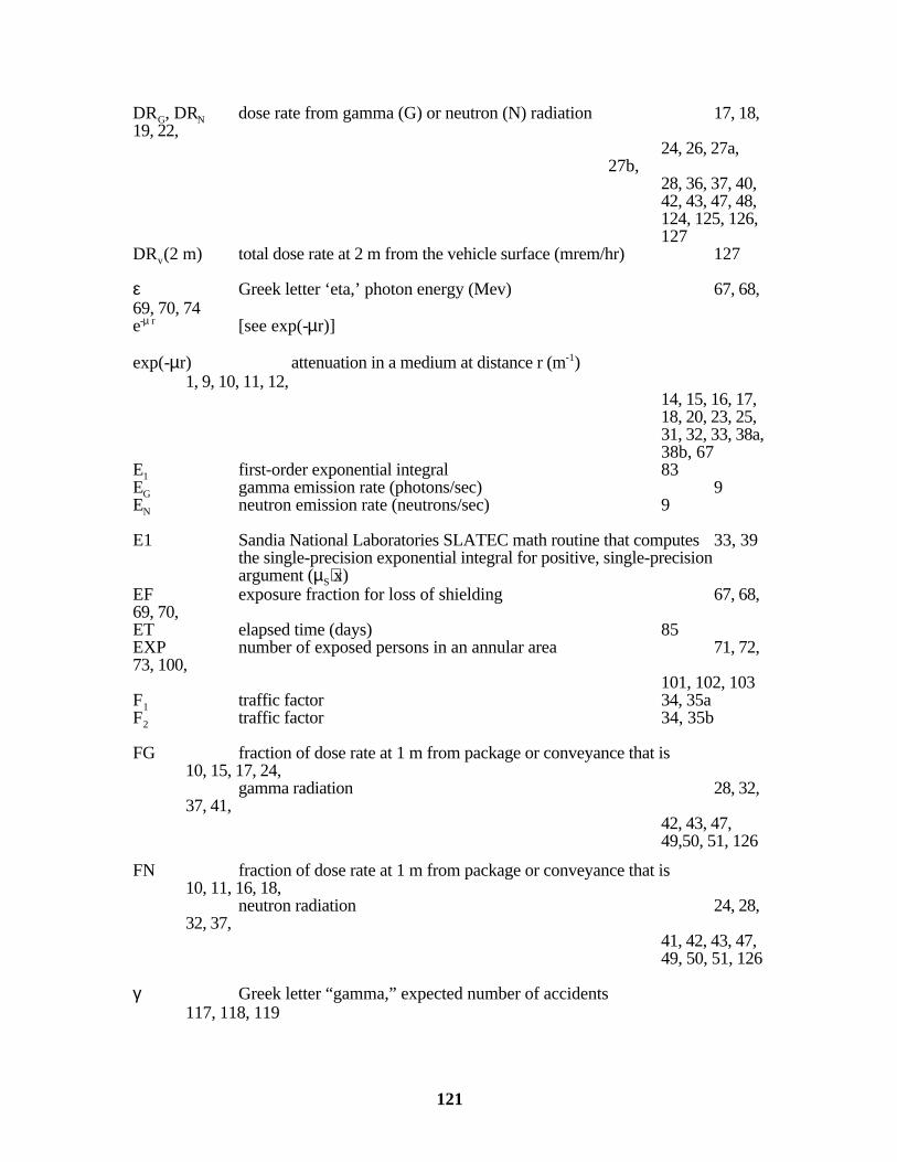
121

DRG, DRN dose rate from gamma (G) or neutron (N) radiation 17, 18,19, 22,

24, 26, 27a,27b,

28, 36, 37, 40,42, 43, 47, 48,124, 125, 126,127

DRv(2 m) total dose rate at 2 m from the vehicle surface (mrem/hr) 127

ε Greek letter ‘eta,’ photon energy (Mev) 67, 68,69, 70, 74e-µ r [see exp(-µr)]

exp(-µr) attenuation in a medium at distance r (m-1)1, 9, 10, 11, 12,

14, 15, 16, 17,18, 20, 23, 25,31, 32, 33, 38a,38b, 67

E1 first-order exponential integral 83EG gamma emission rate (photons/sec) 9EN neutron emission rate (neutrons/sec) 9

E1 Sandia National Laboratories SLATEC math routine that computes 33, 39the single-precision exponential integral for positive, single-precisionargument (µS⋅x)

EF exposure fraction for loss of shielding 67, 68,69, 70,ET elapsed time (days) 85EXP number of exposed persons in an annular area 71, 72,73, 100,

101, 102, 103F1 traffic factor 34, 35aF2 traffic factor 34, 35b

FG fraction of dose rate at 1 m from package or conveyance that is10, 15, 17, 24,

gamma radiation 28, 32,37, 41,

42, 43, 47,49,50, 51, 126

FN fraction of dose rate at 1 m from package or conveyance that is10, 11, 16, 18,

neutron radiation 24, 28,32, 37,

41, 42, 43, 47,49, 50, 51, 126

γ Greek letter “gamma,” expected number of accidents 117, 118, 119

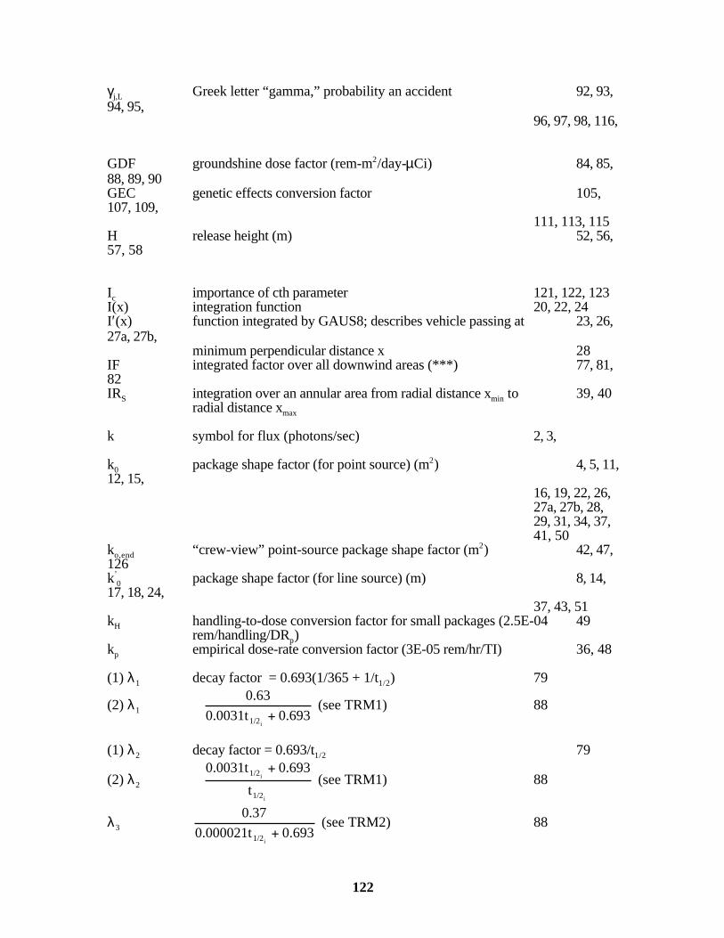
122

γj,L Greek letter “gamma,” probability an accident 92, 93,94, 95,

96, 97, 98, 116,

GDF groundshine dose factor (rem-m2/day-µCi) 84, 85,88, 89, 90GEC genetic effects conversion factor 105,107, 109,

111, 113, 115H release height (m) 52, 56,57, 58

Ic importance of cth parameter 121, 122, 123I(x) integration function 20, 22, 24I′(x) function integrated by GAUS8; describes vehicle passing at 23, 26,27a, 27b,

minimum perpendicular distance x 28IF integrated factor over all downwind areas (***) 77, 81,82IRS integration over an annular area from radial distance xmin to 39, 40

radial distance xmax

k symbol for flux (photons/sec) 2, 3,

k0 package shape factor (for point source) (m2) 4, 5, 11,12, 15,

16, 19, 22, 26,27a, 27b, 28,29, 31, 34, 37,41, 50

ko,end “crew-view” point-source package shape factor (m2) 42, 47,126k’

0 package shape factor (for line source) (m) 8, 14,17, 18, 24,

37, 43, 51kH handling-to-dose conversion factor for small packages (2.5E-04 49

rem/handling/DRp)kp empirical dose-rate conversion factor (3E-05 rem/hr/TI) 36, 48

(1) λ1 decay factor = 0.693(1/365 + 1/t1/2) 79

(2) λ1 0.6930.0031t

0.63

i1/2

(see TRM1) 88

(1) λ2 decay factor = 0.693/t1/2 79

(2) λ2

i

i

1/2

1/2

t

0.693 0.0031t (see TRM1) 88

λ3 693.00.000021t

0.37

i1/2

(see TRM2) 88

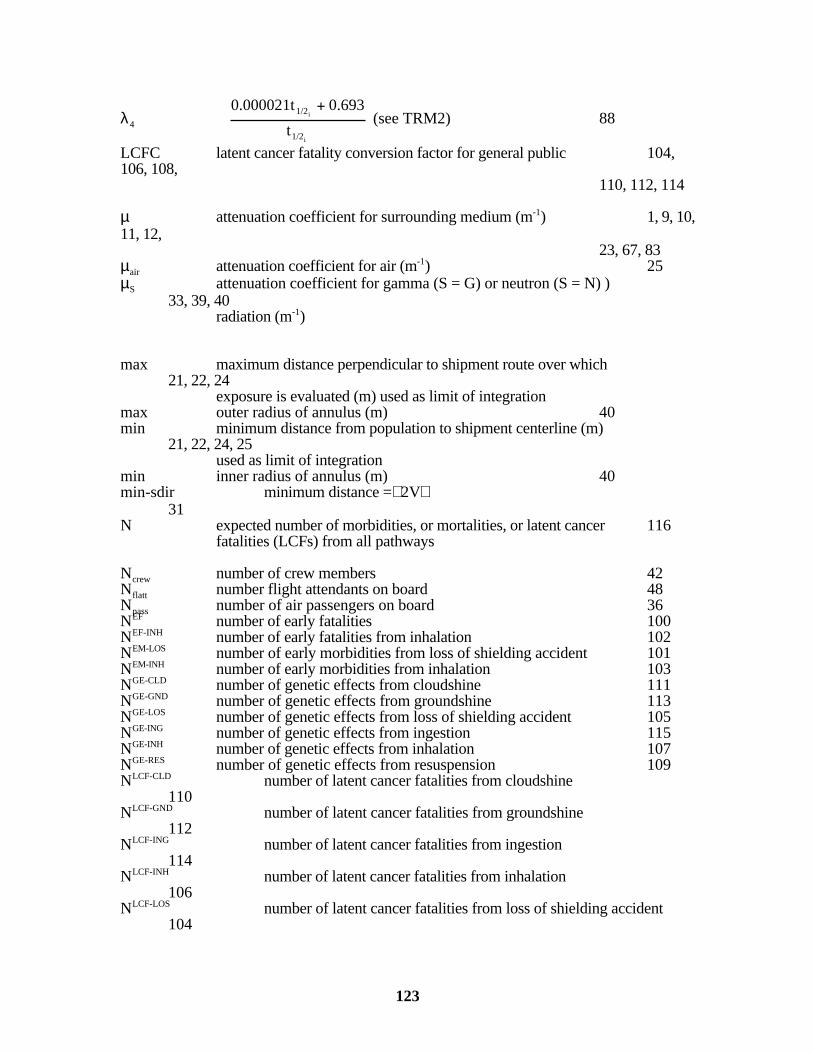
123

λ4

i

i

1/2

1/2

t

0.693 0.000021t (see TRM2) 88

LCFC latent cancer fatality conversion factor for general public 104,106, 108,

110, 112, 114

µ attenuation coefficient for surrounding medium (m-1) 1, 9, 10,11, 12,

23, 67, 83µair attenuation coefficient for air (m-1) 25µS attenuation coefficient for gamma (S = G) or neutron (S = N) )

33, 39, 40radiation (m-1)

max maximum distance perpendicular to shipment route over which21, 22, 24

exposure is evaluated (m) used as limit of integrationmax outer radius of annulus (m) 40min minimum distance from population to shipment centerline (m)

21, 22, 24, 25used as limit of integration

min inner radius of annulus (m) 40min-sdir minimum distance =2V

31N expected number of morbidities, or mortalities, or latent cancer 116

fatalities (LCFs) from all pathways

Ncrew number of crew members 42Nflatt number flight attendants on board 48Npass number of air passengers on board 36NEF number of early fatalities 100NEF-INH number of early fatalities from inhalation 102NEM-LOS number of early morbidities from loss of shielding accident 101NEM-INH number of early morbidities from inhalation 103NGE-CLD number of genetic effects from cloudshine 111NGE-GND number of genetic effects from groundshine 113NGE-LOS number of genetic effects from loss of shielding accident 105NGE-ING number of genetic effects from ingestion 115NGE-INH number of genetic effects from inhalation 107NGE-RES number of genetic effects from resuspension 109NLCF-CLD number of latent cancer fatalities from cloudshine

110NLCF-GND number of latent cancer fatalities from groundshine

112NLCF-ING number of latent cancer fatalities from ingestion

114NLCF-INH number of latent cancer fatalities from inhalation

106NLCF-LOS number of latent cancer fatalities from loss of shielding accident

104

124

NLCF-RES number of latent cancer fatalities from resuspension10

N′ one-way traffic count (average number of vehicles per hour 27a,27b, 28, 31

in all lanes)NL′ traffic count on link L 34NCL number of rail classifications per trip 44, 45

NE neutron emission factor (neutrons/sec-Ci) 75NRAD number of annular areas 68, 71,100NSH number of shipments 24, 27a, 27b,28,

36NSHL number of shipments on link L 30, 92,119NSHv number of shipments by conveyance v 34, 37,41, 42,

43, 47, 48, 49,50, 51

π Greek letter ‘pi;’ = 3.1415 1, 3, 41,52, 53,

54, 55, 56, 57,58, 69, 70, 72,73, 75

φ Greek letter ‘phi,’ uncollided flux (photons/cm2/sec) 83Pst average number of exposed persons at stop 37PEF probability of early fatality 100, 102PEM probability of early morbidity 101, 103PV,G or PV,N form of integral from Equation 31

PD population density (persons/km2) 21, 22,69, 70,

71, 72, 73PDL population density on link L (persons/km2) 24, 77,81, 82,

88, 89, 90PDst population density at a stop (persons/km2) 41PPS number of packages per shipment 49, 50,51, 67,

68, 69, 70, 74,75, 76, 77, 80,81, 82, 86, 89,90

PPV vehicle occupancy (ave. number of persons per vehicle) 27a,27b, 31PPVL vehicle occupancy on link L 28, 34

(1) Q units conversions factor 4, 7, 11,12, 14,

21, 67(2) Q rate of release of dispersed substance (Ci/sec) 52, 53, 54, 55,

125

56, 57, 58

Q1 units conversion factor = 2.8E-10 rem-km-hr/mrem-m-sec 15, 16,17, 18,

22, 24, 42, 43Q2 units conversion factor = 7.7E-08 rem-hr2-m/mrem-sec2-km. 28, 34Q3 units conversion factor = 0.28 m-hr/km-sec 36, 48Q4 units conversion factor = 1.0E-03 rem/mrem 37, 41,50, 51Q5 units conversion factor = 2.0E-07 m-hr-day/km-sec-min 47Q6 units conversion factor = 0.5 rem-m/hr-Ci-Mev 68, 69,70, 74Q7 units conversion factor = 1.0E-06 km2/m2 69, 70,71, 72,

73, 77, 81, 82,88, 89, 90

Q8 units conversion factor 1.0E-06 m2/cm2 75Q9 units conversion factor = 1.0E+6 µCi/Ci 86

r radial distance from point source (m) 1, 2, 4, 7, 9, 10,11, 12, 14, 15,

1617, 18, 20, 23,25, 29, 32, 67,

6970, 83

rend source-to-worker distance for truck crew members (m) 42, 126rk radial distance from source for annular area determination (m)

68, 71, 72, 73,74, 75

rst average radial source-to-receptor distance at stops (m) 37

R ratio of unshielded and shielded cases for calculation of 25off-link dose

RS railyard worker dose factor for gamma (S = G) and neutron (S = N) 43RDF resuspension dose factor 78, 79RESP respirable fraction 76, 77,RF release fraction 76, 77, 80, 81,

82RISKHE health-effects risk

116RISKCLD cloudshine dose-risk 96, 99RISKGND groundshine dose-risk 97, 99RISKING ingestion dose-risk 98RISKINH inhalation dose-risk 94, 99RISKLOS dose-risk for loss of shielding 93RISKRES resuspension dose-risk

95, 99RISKTOTAL total dose-risk from dispersion 99RPC dose conversion factor (rem/Ci) 76, 77,RPDs or u ratio of pedestrian density to residential population density in

24, 69, 70, 71, 82suburban (s) or urban (u) route segments.

126

RU building shielding factor for urban areas 72

σy crosswind meteorological constant (m) 52, 53,54, 55,

56, 57, 58σz vertical meteorological constant (m) 52, 53, 54, 55,

56, 57, 58S source strength (photons/cm2/sec) 83Sphoton particle or photon emission rate (photons/sec) 1, 3

2

photon

r 4

Sflux at distance r (photons/sec/cm2) 1

SEG number of segments per annulus = 8 71

SF shielding factor 24SFp shielding factor in population zone p 69, 70,SFst shielding factor for stop population 37, 41

SVj,L fraction of accidents of severity j on link L 92sw sidewalk width (m); used as a limit of integration 24SWALK width of sidewalk (m) 71t exposure time for on-link dose calculation 29, 30t1/2 half-life (days) 85, 88, 89, 90T exposure time (hr) 69, 70, 74, 75TE time before evacuation begins (days) (see TRM1) 88TH average exposure time of handlers (hr) 50, 51TS survey time (days) (see TRM2) 88Tst average stop time (hr) 37, 41

TDF total decontamination factor 87

TRG term for gamma radiation source strength at distance r 37, 38a,42, 43,

49, 50, 51TRG,2 dose-distance relationship factor at 2 m for gamma radiation 47TRG,r dose-distance relationship factor at r m for gamma radiation 126TRN term for neutron radiation source strength at distance r 37,38b, 42, 43,

49, 50, 51TRN,2 dose-distance relationship factor at 2 m for neutron radiation 47TRN,r dose-distance relationship factor at r m for neutron radiation 126

TRM1 )e-(1 )e1( E4E2 T-3

T-1 88, 89, 90

TRM2 = )e-(e e 41.83E-T-3

)T(1

4S4S2 88, 89

u wind speed (m/sec) 52, 53, 54, 55,56, 57, 58

UBF urban fraction of persons indoors 72, 82,USWF urban sidewalk fraction 82

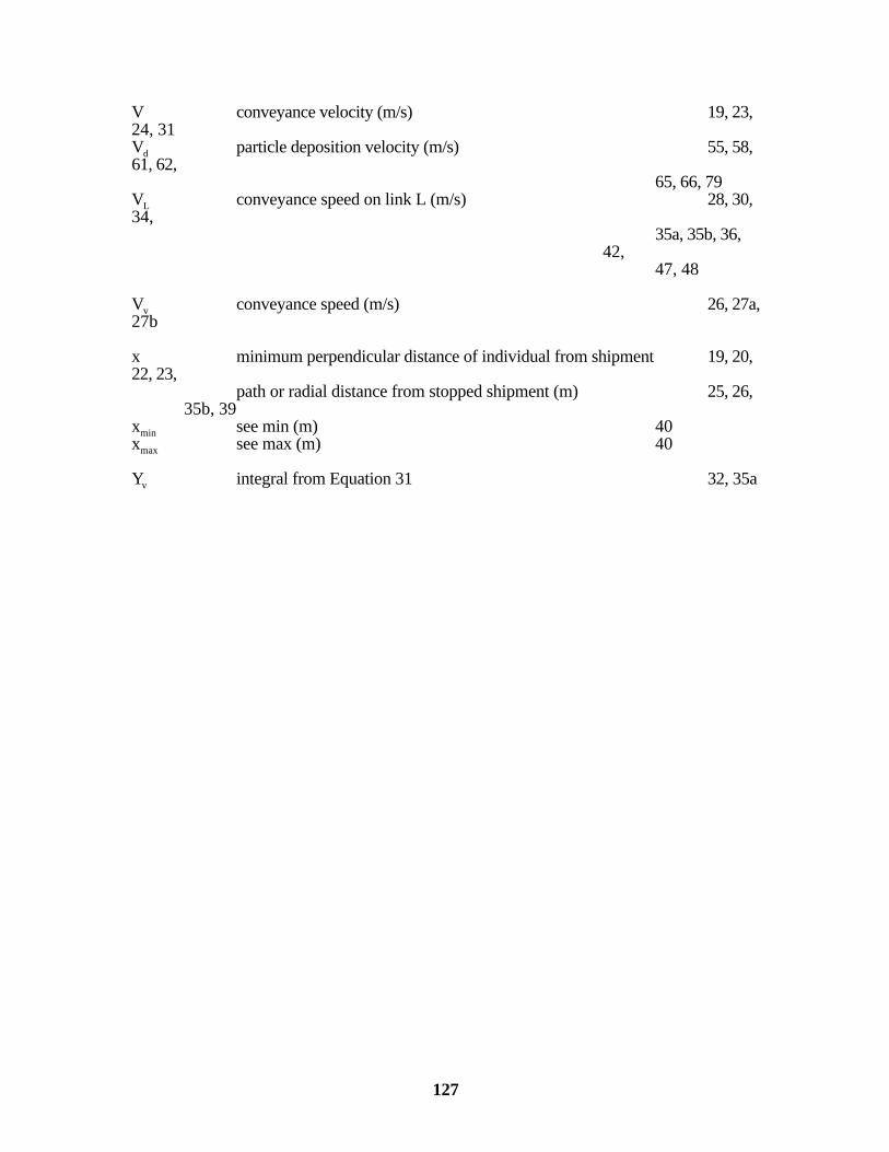
127

V conveyance velocity (m/s) 19, 23,24, 31Vd particle deposition velocity (m/s) 55, 58,61, 62,

65, 66, 79VL conveyance speed on link L (m/s) 28, 30,34,

35a, 35b, 36,42,

47, 48

Vv conveyance speed (m/s) 26, 27a,27b

x minimum perpendicular distance of individual from shipment 19, 20,22, 23,

path or radial distance from stopped shipment (m) 25, 26,35b, 39

xmin see min (m) 40xmax see max (m) 40

Yv integral from Equation 31 32, 35a

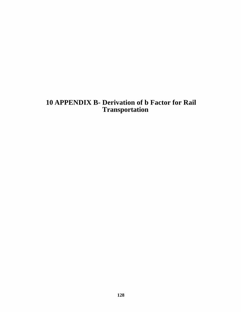
128

10 APPENDIX B- Derivation of b Factor for RailTransportation

129

10.1 Introduction

This appendix documents the derivation of the factors b1 through b11 that are used incalculating incident-free dose to rail workers (Section 3.5.2, Equation 43).

The b factors were developed from time and motion data reported in Wooden (1986). Wooden conducted “a detailed analysis of rail operations that are important for assessingthe risk of transporting high-level nuclear waste.” Wooden identified three categories ofactivities that take place in rail operations, mainly in railyards, during which rail workersroutinely would come into proximity to a spent-fuel shipment or similar large-quantity TypeB shipment. These activity categories are:• Classification• Repair• Inspection.

The emphasis of the Wooden report was on “general freight” shipments, which includesall three categories. Only Inspection is routinely practiced for dedicated rail shipments. Foreach operation in a category, Wooden estimated the average number of person-hoursnecessary to perform a task and the average distance from a hypothetical RAM car. Wooden derived these values from actual observations of worker numbers and elapsedtimes. In some cases, elapsed time was determined by velocity of the railcar(s). Theresulting values, given below, give person-hours for each task and average worker distance. At all distances except 20 m, a line-source formulation is applied; at 20 m a point-sourceformulation is required. The units of b are person-hr/m in all cases, however, so the k0 inthe usual point-source formulation was set equal to 3.5 0k′ and the 20-m case was treatedmathematically in the same manner as a line-source (Wooden, 1986, Appendix A).

Section B.2 contains tables that list the person-hours and distances for each step in each offour possible classification operations. The type of classification operation actually useddepends on the layout of the railyard. Section B.3 describes similar steps for performing arailcar inspection; and Section B.4 addresses the four types of railcar-repair facilities. Finally, in Section B.5, b factors are derived from the foregoing data.

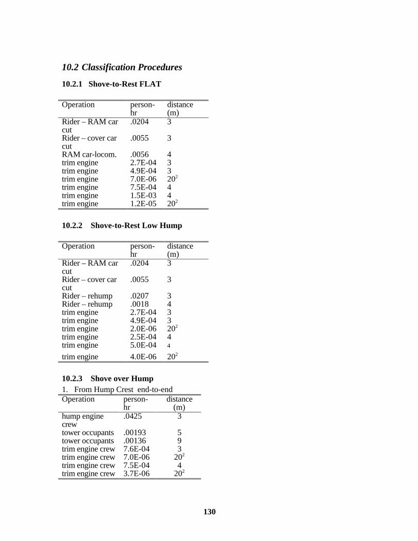
130

10.2 Classification Procedures

10.2.1 Shove-to-Rest FLAT

Operation person-hr

distance(m)

Rider – RAM carcut

.0204 3

Rider – cover carcut

.0055 3

RAM car-locom. .0056 4trim engine 2.7E-04 3trim engine 4.9E-04 3trim engine 7.0E-06 202

trim engine 7.5E-04 4trim engine 1.5E-03 4trim engine 1.2E-05 202

10.2.2 Shove-to-Rest Low Hump

Operation person-hr

distance(m)

Rider – RAM carcut

.0204 3

Rider – cover carcut

.0055 3

Rider – rehump .0207 3Rider – rehump .0018 4trim engine 2.7E-04 3trim engine 4.9E-04 3trim engine 2.0E-06 202

trim engine 2.5E-04 4trim engine 5.0E-04 4

trim engine 4.0E-06 202

10.2.3 Shove over Hump1. From Hump Crest end-to-endOperation person-

hrdistance

(m)hump enginecrew

.0425 3

tower occupants .00193 5tower occupants .00136 9trim engine crew 7.6E-04 3trim engine crew 7.0E-06 202

trim engine crew 7.5E-04 4trim engine crew 3.7E-06 202

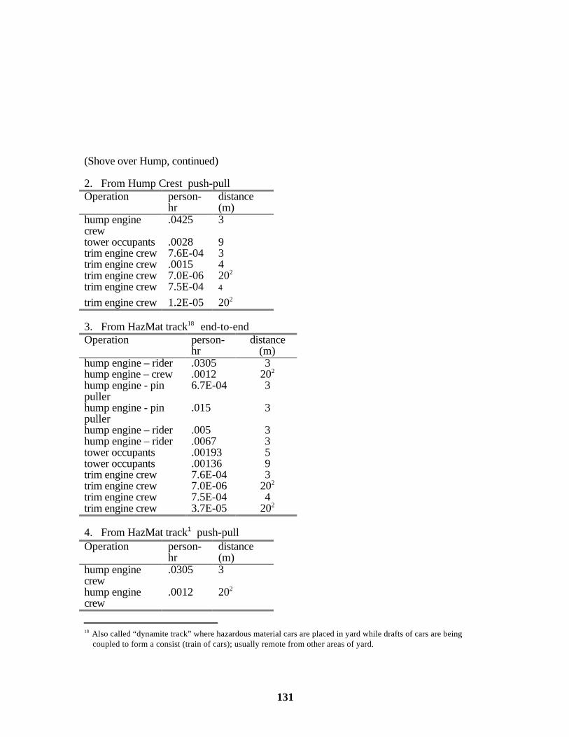
131

(Shove over Hump, continued)

2. From Hump Crest push-pullOperation person-

hrdistance(m)

hump enginecrew

.0425 3

tower occupants .0028 9trim engine crew 7.6E-04 3trim engine crew .0015 4trim engine crew 7.0E-06 202

trim engine crew 7.5E-04 4

trim engine crew 1.2E-05 202

3. From HazMat track18 end-to-endOperation person-

hrdistance

(m)hump engine – rider .0305 3hump engine – crew .0012 202

hump engine - pinpuller

6.7E-04 3

hump engine - pinpuller

.015 3

hump engine – rider .005 3hump engine – rider .0067 3tower occupants .00193 5tower occupants .00136 9trim engine crew 7.6E-04 3trim engine crew 7.0E-06 202

trim engine crew 7.5E-04 4trim engine crew 3.7E-05 202

4. From HazMat track1 push-pullOperation person-

hrdistance(m)

hump enginecrew

.0305 3

hump enginecrew

.0012 202

18 Also called “dynamite track” where hazardous material cars are placed in yard while drafts of cars are being

coupled to form a consist (train of cars); usually remote from other areas of yard.

132

hump enginecrew

.02737 3

tower occupants .0028 9trim engine crew 7.6E-04 3trim engine crew 7.0E-06 202

trim engine crew 7.5E-04 4trimengine crew .0015 4trim engine crew 1.2E-05 202

10.2.4 Shove from Trim End1. Shove from trim end; from hump crest; end-to-endOperation person-hr distance

(m)hump personnel .0186 (p. 65) 5hump personnel .0131 (p. 65) 9hump personnel 5.9E-04 (p.

49)3

hump personnel 4.4E-04 (p.49)

4

hump personnel 9.5E-04 (p.51)

4

tower occupants .00193 5tower occupants .00136 9trim engine - classifying(rider)

.0383 (p.65) 3

trim engine – classifying(crew)

.1189 4

trim engine – assembly .00954 3trim engine – assembly .00938 4trim engine – assembly .00102 (p.

54)202

2. Shove from trim end; from hump crest push-pullOperation person-hr distance

(m)hump personnel .0334 (p. 65) 9hump personnel -pin puller .0012 (p. 49) 3hump personnel - pin puller 9.0E-04 (p.55) 4hump personnel .0019 (p. 51 & 4

133

55)hump personnel .0028 (p. 55) 9trim engine – classifying(rider)

.0383 (p. 65) 3

trim engine – classifying(crew)

.1189 4

trim engine – assembly .00954 3trim engine – assembly .00039 202

trim engine – assembly .0469 4

3. Shove from trim end; from HazMat track; end-to-endOperation person-hr distance

(m)hump personnel – shoving–cab

.0500 (p.66) 3

hump personnel – shoving –cab

.0750 (p.66) 4

hump personnel – cut .00067 (p.67)

3

hump personnel – placement .015 (p. 67) 3hump personnel – pickup .0075 (p.

67)3

hump personnel – cab .01125 (p.67)

4

tower occupants .00193 5tower occupants .00136 9trim engine – classifying(rider)

.0383 (p. 65) 3

trim engine – classifying(crew)

.0439 (p. 66) 4

trim engine – assembly .00954 3trim engine – assembly .00938 4trim engine – assembly .00102 202

(Shove from Trim End, continued)

4. Shove from trim end; from HazMat track; push-pullOperation person-hr distance

(m)hump personnel – shoving–cab

.0500 (p.66) 3

hump personnel – shoving –cab

.0750 (p.66) 4

hump personnel – cut .6.7E-04 (p.67)

3

hump personnel – placement .015 (p. 67) 3hump personnel – pickup .0075 (p. 67) 3hump personnel – cab .01125 (p. 67) 4

134

tower occupants .0028 (p.55) 9trim engine – classifying(rider)

.0383 (p. 65) 3

trim engine – classifying(crew)

.0439 (p. 66) 4

trim engine – assembly .00954 3trim engine – assembly .0469 4trim engine – assembly 3.9E-04 202

10.3 Inspection

Operation person-hr

distance(m)

RAM train inspection .0220 3Adjacent track inspection –nearside

.0078 4

Adjacent track inspection – farside

.0025 8

Inspection 2 tracks away .0030 9

135

10.4 Repairs

1. Large Intermediate Terminal - One Spot Repair Facility (Wooden, p. 73-75)

Operation person-hr

distance(m)

Repair in coveredfacility

.0077 3

Repair in coveredfacility

.0046 5

Repair in coveredfacility

.0029 5

Repair on cleaningtracks

.0012 3

Repair on cleaningtracks

.0008 5

Repair in arrival yard .0083 3Repair in arrival yard .0058 5Repair in arrival yard .0017 3Repair in arrival yard .0012 5

2. Very Large Intermediate Terminal - One Spot Repair Facility (Wooden, p. 73, 75, & 77)

Operation person-hr

distance(m)

Repair in coveredfacility

.0111 3

Repair in coveredfacility

.0067 5

Repair in coveredfacility

.0042 5

Mini rip track .0037 3Mini rip track .0026 5

3. Interchange Terminal – One Spot Repair Facility (p. 73 & 77)

Operation person-hr

distance(m)

Repair in coveredfacility

.0233 3

Repair in coveredfacility

.014 5

Repair on adjacenttrack

.0089 5

4. Small Terminal – Rip Track Repair Facility (3 parallel tracks) p. 77 & 78)

136

Operation person-hr

distance(m)

Repair on RAM car .0132 3Repair on adjacent car .0091 5Repair on adjacent track(near)

.0050 7

Repair on adjacent track(far)

.0043 9

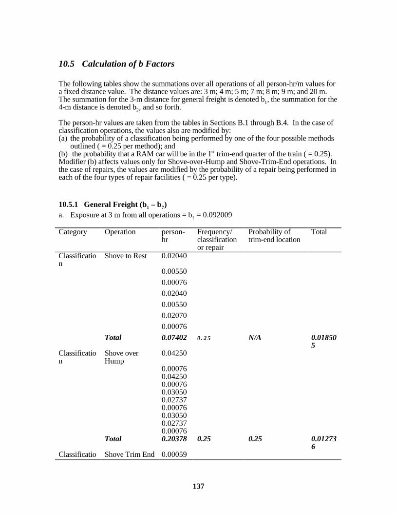
137

10.5 Calculation of b Factors

The following tables show the summations over all operations of all person-hr/m values fora fixed distance value. The distance values are: 3 m; 4 m; 5 m; 7 m; 8 m; 9 m; and 20 m. The summation for the 3-m distance for general freight is denoted b1, the summation for the4-m distance is denoted b2, and so forth.

The person-hr values are taken from the tables in Sections B.1 through B.4. In the case ofclassification operations, the values also are modified by:(a) the probability of a classification being performed by one of the four possible methods

outlined ( = 0.25 per method); and(b) the probability that a RAM car will be in the 1st trim-end quarter of the train ( = 0.25). Modifier (b) affects values only for Shove-over-Hump and Shove-Trim-End operations. Inthe case of repairs, the values are modified by the probability of a repair being performed ineach of the four types of repair facilities ( = 0.25 per type).

10.5.1 General Freight (b1 – b7)a. Exposure at 3 m from all operations = b1 = 0.092009

Category Operation person-hr

Frequency/classificationor repair

Probability oftrim-end location

Total

Classification

Shove to Rest 0.02040

0.00550

0.00076

0.02040

0.00550

0.02070

0.00076

Total 0.07402 0 . 2 5 N/A 0.018505

Classification

Shove overHump

0.04250

0.000760.042500.000760.030500.027370.000760.030500.027370.00076

Total 0.20378 0.25 0.25 0.012736

Classificatio Shove Trim End 0.00059

138

n0.038300.009540.001200.038300.009540.050000.023170.038300.009540.050000.023170.038300.00954

Tota l 0.33949 0.25 0.25 0.021218

Inspection Inspection 0.0220 0.022

Tota l 0.0220 1 N/A 0.022Repairs Repairs 0.0077

0.0012

0.00830.00170.01110.00370.02330.0132

Total .0702 0.25 N/A 0.01755TOTAL .092009

139

b. Exposure at 4 m from all operations = b2 = 0.049201

Category Operation person-hr

Frequency/classification or repair

Probability of trim-end location

Total

Classification

Shove-to-Rest 0.00560

0.000750.001500.001800.00075

Total 0.01040 0.25 N/A 0.0026Classification

Shove overHump

0.00075

0.00075

0.001500.00075

0.000750.00150

Total 0.0060 0.25 0.25 0.000375

Classification

Shove Trim End 0.00044

0.000950.118900.009380.000900.001900.118900.046900.075000.011250.043900.009360.075000.01125

0.043900.04690

Total 0.61483 0.25 0.25 0.038426

Inspection Inspection 0.0078

Total 0.0078 N/A N/A 0.007800

140

TOTAL 0.049201

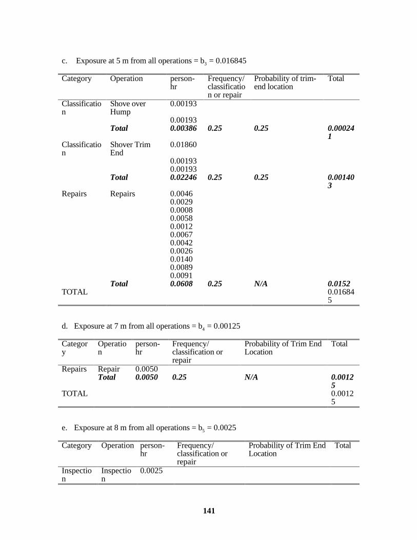
141

c. Exposure at 5 m from all operations = b3 = 0.016845

Category Operation person-hr

Frequency/classification or repair

Probability of trim-end location

Total

Classification

Shove overHump

0.00193

0.00193Total 0.00386 0.25 0.25 0.00024

1Classification

Shover TrimEnd

0.01860

0.001930.00193

Total 0.02246 0.25 0.25 0.001403

Repairs Repairs 0.00460.00290.00080.00580.00120.00670.00420.00260.01400.00890.0091

Total 0.0608 0.25 N/A 0.0152TOTAL 0.01684

5

d. Exposure at 7 m from all operations = b4 = 0.00125

Category

Operation

person-hr

Frequency/classification orrepair

Probability of Trim EndLocation

Total

Repairs Repair 0.0050Total 0.0050 0.25 N/A 0.0012

5TOTAL 0.0012

5

e. Exposure at 8 m from all operations = b5 = 0.0025

Category Operation person-hr

Frequency/classification orrepair

Probability of Trim EndLocation

Total

Inspection

Inspection

0.0025

142

Total 0.0025 N/A N/A 0.0025TOTAL 0.0025

143

Exposure at 9 m from all operations = b6 = .008023

Category Operation person-hr

Frequency/classification orrepair

Probability ofTrim EndLocation

Total

Classification

Shove overHump

0.00136

0.002800.001360.00280

Total 0.00832 0.25 0.25 0.00052Classification

Shove Trim End 0.01313

0.001360.033400.00280

0.001360.00280

Total 0.05485 0.25 0.25 0.003428

Inspection Inspection 2tracks away

0.0030

Total 0.0030 N/A N/A 0.0030Repairs Repair 0.0043

Total 0.0043 0.25 N/A 0.001075

TOTAL 0.008023

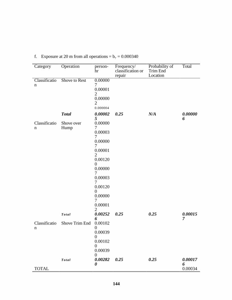
144

f. Exposure at 20 m from all operations = b7 = 0.000340

Category Operation person-hr

Frequency/classification orrepair

Probability ofTrim EndLocation

Total

Classification

Shove to Rest 0.0000070.0000120.0000020.000004

Total 0.000025

0.25 N/A 0.000006

Classification

Shove overHump

0.0000070.0000370.0000070.0000120.0012000.0000070.0000370.0012000.0000070.000012

Tota l 0.002526

0.25 0.25 0.000157

Classification

Shove Trim End 0.0010200.0003900.0010200.000390

Tota l 0.002820

0.25 0.25 0.000176

TOTAL 0.00034

145

0

10.5.2 B.5.2 Dedicated Rail (b8 – b11)

For dedicated rail, only exposures from inspections are included because the consist (trainof cars) is not broken down and reassembled at each railyard as it is for ordinary freight. Thus, there are no proximate worker exposures associated with classification operations inrailyards. Further, only emergency repairs are performed in the course of dedicated railtransportation.

a. Exposure at 3 m from inspections = b8 = 0.022

Category Operation person-hr

Frequency/classification or repair

Probability of trim-endlocation

Total

Inspection

Inspection 0.0220 0.022

Tota l 0.0220 N/A N/A 0.022TOTAL 0.022

b. Exposure at 4 m from inspections = b9 = 0.0078

Category Operation person-hr

Frequency/classification orrepair

Probability of trim-endlocation

Total

Inspection

Inspection 0.0078

Total 0.0078 N/A N/A 0.0078TOTAL 0.0078

c. Exposure at 8 m from inspections = b10 = 0.0025

Category Operation person-hr

Frequency/

classification orrepair

Probability of Trim EndLocation

Total

Inspection

Inspection

0.0025

Total 0.0025 N/A N/A 0.0025TOTAL 0.0025

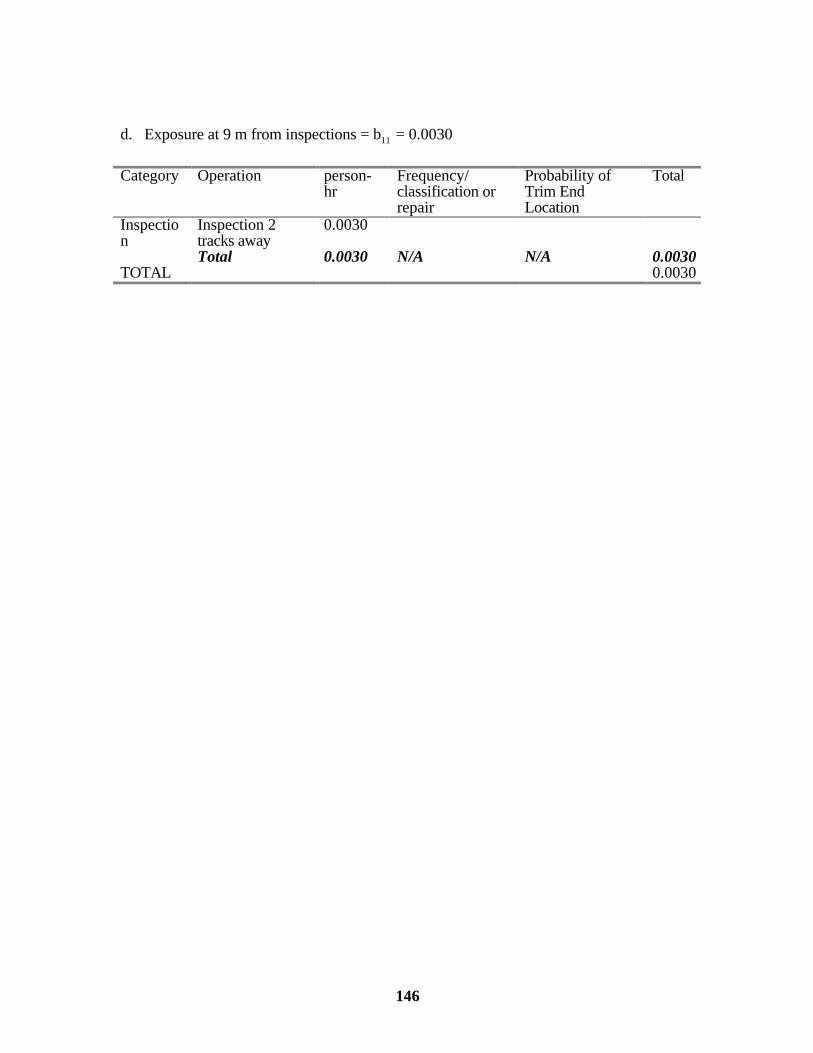
146

d. Exposure at 9 m from inspections = b11 = 0.0030

Category Operation person-hr

Frequency/classification orrepair

Probability ofTrim EndLocation

Total

Inspection

Inspection 2tracks away

0.0030

Total 0.0030 N/A N/A 0.0030TOTAL 0.0030

147

10.6 Literature Cited

Wooden, D.G., 1986, “Railroad Transportation of Spent Nuclear Fuel,” SAND86-7083,Sandia National Laboratories, Albuquerque, NM.

148