Radiosity vs. Ray Tracing Radiosity - MIT CSAILgroups.csail.mit.edu/graphics/classes/6.837/F01/Lecture20/lecture... · Ray Tracing vs. Radiosity Ray tracing is an image-space algorithm,

1

Slide 1Lecture 20 6.837 Fall ‘01

Radiosity

References:

Cohen and Wallace, Radiosity and Realistic Image Synthesis

Sillion and Puech, Radiosity and Global Illumination

Thanks to Leonard McMillan for the slides

Thanks to François Sillion for images

An early application of radiative heat transfer in stables.


Why Radiosity?

A powerful demonstration introduced by Goral et al. of the differences between radiosity and traditional ray tracing is provided by a sculpture by John Ferren. The sculpture consists of a series of vertical boards painted white on the faces visible to the viewer. The back faces of the boards are painted bright colors. The sculpture is illuminated by light entering a window behind the sculpture, so light reaching the viewer first reflects off the colored surfaces, then off the white surfaces before entering the eye. As a result, the colors from the back boards “bleed” onto the white surfaces.

eye


Radiosity vs. Ray Tracing

Original sculpture litby daylight from the rear.

Image rendered with radiosity. note color bleeding effects.

Ray traced image. A standardRay tracer cannot simulate theinterreflection of light between diffuse Surfaces.


Ray Tracing vs. Radiosity

Ray tracing is an image-space algorithm, while radiosity is computed in object-space.

Because the solution is limited by the view, ray tracing is often said to provide a view-dependent solution, although this is somewhat misleading in that it implies that the radiance itself is dependent on the view, which is not the case. The term view-independentrefers only to the use of the view to limit the set if locations and directions for which the radiance is computed.

2


Radiosity Introduction

The radiosity approach to rendering has its basis in the theory of heat transfer. This theory was applied to computer graphics in 1984 by Goral et al.

Surfaces in the environment are assumed to be perfect (or Lambertian) diffusers, reflectors, or emitters. Such surfaces are assumed to reflect incident light in all directions with equal intensity.

A formulation for the system of equations is facilitated by dividing the environment into a set of small areas, or patches. The radiosity over a patch is constant.

The radiosity, B, of a patch is the total rate of energy leaving a surface and is equal to the sum of the emitted and reflected energies:

Radiosity was used for Quake II


Solving the rendering equation

L is the radiance from a point on a surface in a given direction ωE is the emitted radiance from a point: E is non-zero only if x’ is emissiveV is the visibility term: 1 when the surfaces are unobstructed along the direction ω, 0

otherwise G is the geometry term, which depends on the geometric relationship between the two

surfaces x and x’

Photon-tracing uses sampling and Monte-Carlo integrationRadiosity uses finite elements:

project onto a finite set of basis functions (piecewise constant)

Ray tracing computes L [D] S* EPhoton tracing computes L [D | S]* ERadiosity only computes L [D]* E

( ) ( ) ( ) ( ) ( ) ( ), , , ,s

L x E x x L x G x x V x x dAω ρ ω′ ′ ′ ′ ′ ′= + ∫� �


+ ∫

Continuous Radiosity Equation

x

x’

+= xxx’x’ BG(x,x’)V(x,x’)EB ρ

Form factor

•G: geometry term •V: visibility term

•No analytical solution, even for simple configurations

For an environment composed of diffuse surfaces, we have the basic radiosity relationship:

reflectivity

x


Discrete Radiosity Equation

A

iA

j ∑+=j=1

jijiii BFEB ρ

Form factor

• discrete representation• iterative solution• costly geometric/visibilitycalculations

For an environment that has been discretized into n patches, over which the radiosity is constant, (i.e. both B and E are constant across a patch), we have the basic radiosity relationship:

reflectivityn

3


The Radiosity Matrix

A solution yields a single radiosity value Bi for each patch in the environment – a view-independent solution. The Bi values can be used in a standard renderer and a particularview of the environment constructed from the radiosity solution.

1

2

n

BB

B

�

1

2

n

EE

E

�=

1 11 1 12 1 1

2 21 2 22

1

11

1

n

n n n nn

F F FF F

F F

ρ ρ ρρ ρ

ρ ρ

− − − − − − −

�

� �

� �

Such an equation exists for each patch, and in a closed environment, a set of n simultaneousequations in n unknown Bi values is obtained:

iBiB


Standard Solution of the Radiosity Matrix

1

2

1

2

1

1 1

2

i i ii i i i i in

nn n

BB

B E BF

B EB

F F

B

E

B E

ρ ρ ρ

= +

��

� � �

�

�

The radiosity of a single patch i is updated for each iteration by gathering radiosities from all other patches:

This method is fundamentally a Gauss-Seidel relaxation


Computing Vertex Radiosities

�Recall that radiosity values are constant over the extent of a patch.

�A standard renderer requires vertex radiosities (intensities). These can be obtained for a vertex by computing the average of the radiosities of patches that contribute to the vertex under consideration.

�Vertices on the edge of a surface can be allocated values by extrapolation through interior vertex values, as shown on the right:


Stages in a Radiosity SolutionInput of

scene geometry

Input of reflectance properties

Viewing conditions

Visualization

Solution to the systemof equations

Radiosity solution

Form factorcalculation

Radiosity image

4


Progressive Refinement

� The idea of progressive refinement is to provide a quickly rendered image to the user that is then gracefully refined toward a more accurate solution. The radiosity method is especially amenable to this approach.

� The two major practical problems of the radiosity method are the storage costs and the calculation of the form factors.

� The requirements of progressive refinement and the elimination of precalculation and storage of the form factors are met by a restructuring of the radiosity algorithm.

� The key idea is that the entire image is updated at every iteration, rather than a single patch.


Reordering the Solution for PR

Shooting: the radiosity of all patches is updated for each iteration:

1 1 1 1

2 2 2 2

i

i

i

n n n ni

B B FB B F

B

B B F

ρρ

ρ

= +

�

� �

�

�

�

�

� �

�

�

This method is fundamentally a Southwell relaxation


Progressive Refinement Pseudocode

}i;element ofintensity the as B using imagedisplay

0B}

rad;BB rad;BB;B rad

{ element)(every for ;largest is Bthat such i, pick

{ converged)(not while

i

i

jj

jj

i

i

=∆

∆+=∆+∆=∆ρ∗∆=∆

∗∆

jij

i

F

A


Progressive Refinement w/out Ambient Term

5


Progressive Refinement with Ambient Term


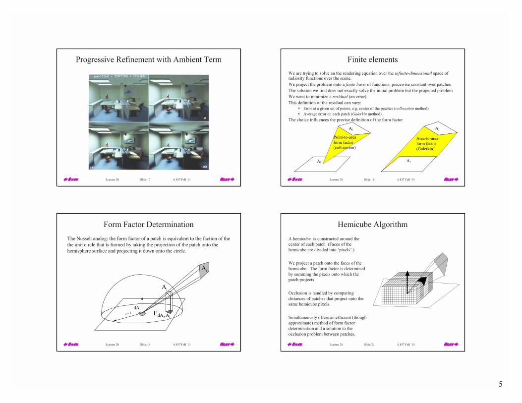
Finite elementsWe are trying to solve an the rendering equation over the infinite-dimensional space of radiosity functions over the scene.We project the problem onto a finite basis of functions: piecewise constant over patchesThe solution we find does not exactly solve the initial problem but the projected problemWe want to minimize a residual (an error).This definition of the residual can vary:

� Error at a given set of points, e.g. center of the patches (collocation method)� Average error on each patch (Galerkin method)

The choice influences the precise definition of the form factor

Ai

Aj

Area-to-area form factor(Galerkin)

Ai

Aj

Point-to-area form factor(collocation)


Form Factor Determination

Aj

Aj

r = 1 FdAi,Aj

dAi

The Nusselt analog: the form factor of a patch is equivalent to the faction of thethe unit circle that is formed by taking the projection of the patch onto the hemisphere surface and projecting it down onto the circle.


Hemicube AlgorithmA hemicube is constructed around the center of each patch. (Faces of thehemicube are divided into ‘pixels’.)

We project a patch onto the faces of the hemicube. The form factor is determined by summing the pixels onto which the patch projects

Occlusion is handled by comparing distances of patches that project onto the same hemicube pixels.

Simultaneously offers an efficient (though approximate) method of form factor determination and a solution to the occlusion problem between patches.

6


Form factor using ray-casting

Cast n rays between the two patches� n is typically between 4 and 32� Compute visibility� Integrate the point-to-point form factor

Monte-Carlo quadrature of the form-factorPermits the computation of the patch-to-patch form factor, as opposed to point-to-patch (i.e. permits Galerkin simulation)

Ai

Aj


Increasing the Accuracy of the Solution

�The quality of the image is a function of the size of the patches.

�In regions of the scene, such as shadow boundaries, that exhibit a high radiosity gradient, the patches should be subdivided. We call this adaptive subdivision.

�The basic idea is as follows:Compute a solution on a uniform initial mesh; the mesh is then refined by subdividing elements that exceed some error tolerance. What’s wrong with this picture?


Adaptive Subdivision of Patches

Coarse patch solution (145 patches)

Improved solution(1021 subpatches)

Adaptive subdivision(1306 subpatches)


Adaptive Subdivision PseudocodeAdaptive_subdivision (error_tolerance) {

Create initial mesh of constant elements;

Compute form factors;Solve linear system;do until (all elements within error tolerance

or minimum element size reached) { Evaluate accuracy by comparing adjacent element radiosities;

Subdivide elements that exceed user-specified error tolerance;for (each new element) {

Compute form factors from new element to all other elements;

Compute radiosity of new element based on old radiosity values;}

}

}

7


Structure of the Solution

� Calculation of form factors(> 90 %)

� Solution to the system of equations( < 10 %)

� Rendering the image(0 %)

Radiosity image

Input of scene geometry

Input of reflectance properties

Viewing conditions

Visualization

Radiosity solution

Solution to the systemof equations

Form factorcalculation


Examples

Factory simulation. Program of Computer Graphics, Cornell University.30,000 patches.


Museum simulation. Program of Computer Graphics, Cornell University.50,000 patches. Note indirect lighting from ceiling.


Lightscape http://www.lightscape.com

8







Combined with ray-tracing


Discontinuity meshing

Limits of umbra and penumbra� Captures nice shadow boundaries� Complex geometric computation� The mesh is getting complex

penumbrapenumbra umbraumbra

sourcesource

blockerblocker

9


Discontinuity meshing


Comparison

[Gibson 96]

With visibilityskeleton & discontinuitymeshing10 minutes 23 seconds 1 hour 57 minutes


Hierarchical approach

Group elements when the light exchange is not important� Breaks the quadratic complexity� Control non trivial, memory cost


Other basis functions

Higher order (non constant basis)� Better representation of smooth variations� Problem: radiosity is discontinuous

Directional basis� For non-diffuse finite elements� E.g. spherical harmonics

10


Next Time: Animation

Documents

Radiosity vs. Ray Tracing Radiosity - MIT CSAILgroups.csail.mit.edu/graphics/classes/6.837/F01/Lecture20/lecture... · Ray Tracing vs. Radiosity Ray tracing is an image-space algorithm,