RRADIO PULSARSADIO PULSARSJoeri van Leeuwen

RA

DIO

PU

LSA

RS

ISBN 90-393-3735-7

RADIO PULSARSRADIO PULSARS(met een samenvatting in het Nederlands)

Proefschrift ter verkrijging van de graad van doctor aan de Universiteit Utrechtop gezag van de Rector Magnificus, Prof. Dr. W.H. Gispen,

ingevolge het besluit van het College voor Promoties in het openbaar te verdedigen opmaandag 10 mei 2004 des middags te 2.30 uur

door

Albert Gerardus Johannes van Leeuwen

geboren op 11 januari 1975, te Waardenburg

Promotor:

Promotiecommissie:

Dit onderzoek werd mede mogelijk gemaakt door de Nederlandse organisatie voor wetenschappelijk onderzoek NWO.

Prof. Dr. F.W.M. VerbuntFaculteit Natuur- en Sterrenkunde, Universiteit Utrecht

Prof. Dr. Ir. J.A.M. BleekerProf. Dr. J. HeiseProf. Dr. E.P.J. van den HeuvelProf. Dr. M.B.M. van der KlisProf. Dr. J. Kuijpers

12345678

Nederlandse inleiding en samenvattingIntroductionNull-induced mode changes in PSR B0809+74Probing drifting and nulling mechanisms through their interaction in PSR B0809+74Intermittent nulls in PSR B0818-13, and the subpulse-drift alias modeUnusual subpulse modulation in PSR B0320+39Pulsar drifting-subpulse polarization: No evidence for systematic polarization-angle rotations|V|: New insight into the circular polarization of radio pulsarsMagnetic field decay versus period-dependent beamingFinding pulsars with LofarBibliographyDank jullie wel - ThanksCurriculum vitae

19

13253545576573839399

101

CONTENTSINHOUD-

NEDERLANDSE INLEIDING EN SAMENVATTINGNEDERLANDSE INLEIDING EN SAMENVATTING

3

Radio pulsars blijven over als sterren aan het eind van hun leven ontploffen. Zelijken nauwelijks nog op de sterren waar ze uit ontstaan: radio pulsars zijn wel evenzwaar als sterren, maar bij de ontploffing zijn ze zo samengeperst dat ze 100.000 keerkleiner zijn geworden. Verder maken radio pulsars vooral radiostraling, terwijl sterrenvooral licht maken.

De afgelopen jaren heb ik onderzocht hoe pulsars radiostraling maken, hoe zeveranderen als ze ouder worden en hoe je zoveel mogelijk nieuwe pulsars kunt ont-dekken met verschillende radiotelescopen. Dat onderzoek wordt in de rest van ditproefschrift specifiek en uitgebreid beschreven. Hier geef ik een wat algemenere in-leiding en vat ik de belangrijkste resultaten samen.

Ik begin met de ontdekking van de eerste radio pulsar, veertig jaar geleden.Daarna zien we dat radio pulsars bij de ontploffing van bepaalde sterren ontstaan.Niet alle sterren worden radio pulsars. Ik vertel ook hoe de andere sterren eindigen:sommige worden ‘witte dwergsterren’, de resterende worden ‘zwarte gaten’. Net alsradio pulsars blijken die allebei te zijn gemaakt van bijna onvoorstelbaar zwaar materi-aal. Ik ga wat dieper in op de bijzondere eigenschappen van radio pulsars en beschrijften slotte wat ik in mijn eigen onderzoek voor nieuws heb gevonden.

Hoe onderzoek je sterren?

Bij onderzoek aan sterren is er een altijd terugkomend probleem: sterren staan zover weg dat je ze niet in detail kunt bekijken. Alleen uit het beetje licht dat ze onzekant op stralen, kunnen we leren hoe sterren werken. Dat begint heel eenvoudig: alsje ’s avond naar de sterrenhemel kijkt, zijn sommige sterren wat roder van kleur enandere wat witter. Dat kleurverschil vertelt je iets over de temperatuur van de ster:de rode zijn redelijk heet (roodgloeiend) maar de witte zijn heter (witheet). Zo kunje met je blote oog al iets te weten komen over een ster. Naast ‘licht’ (de straling dieje kunt zien met je oog) zenden sterren ook nog andere soorten straling uit, zoalsradiostraling, infraroodstraling, ultravioletstraling en rontgenstraling. Al deze soortenstraling lijken erg veel op gewoon licht, alleen zijn onze ogen er niet gevoelig voor.

Figuur 1. Iedere keer als een van de bundels radiostraling over de aarde zwiept, zie je een flits.

Om die straling toch op te kunnen vangen, gebruiken we apparaten als radioantennes,infraroodcamera’s en rontgenfoto’s. Wanneer je met deze apparaten bijvoorbeeld naaronze eigen zon (de dichtstbijzijnde ster) kijkt, krijg je vrijwel hetzelfde plaatje van dezon als met je oog.

In tegenstelling tot sterren maken radio pulsars eigenlijk alleen maar radiostralingen je kunt ze dus niet met het blote oog of een gewone telescoop zien. Daaromduurde het ook lang voor ze ontdekt werden.

Hoe zijn radio pulsars ontdekt?

Eind jaren ’60 werd er in Engeland een nieuwe radiotelescoop gebouwd, gewoon eengroot veld vol radioantennes, allemaal met elkaar verbonden. Met die telescoop werdde hemel afgezocht naar sterren (alleen of in grote groepen ver weg) die radiostralingmaken. Zoals wij sterren zien als lichtpunten aan de hemel, zo ‘ziet’ een radiotele-scoop sterren als radiostralingspunten aan de hemel. Na een paar maanden waren er alveel radiostralingspunten gevonden. De meeste waren altijd even fel (dat bleken heelgrote groepen sterren te zijn, heel ver weg), andere werden ieder paar weken felleren minder fel (dit waren sterren als de zon, niet zo ver weg). Maar er was ook eenpunt dat snel knipperde, ongeveer een keer per seconde. Dat is vreemd, want sterrenkunnen helemaal niet zo snel veranderen, daar zijn ze veel te groot voor. De zon isbijvoorbeeld al 100 keer zo groot als de aarde.

Het was snel duidelijk dat er iets nieuws was ontdekt, al wist nog niemand precieswat. Vanwege de pulserende radiostraling werd het onbekende ding ‘radio pulsar’gedoopt. De meest waarschijnlijke, maar even schokkende uitleg was dat er eindelijksignalen van buitenaardse wezens waren ontdekt, die probeerden contact met ons temaken. Een tijdje geleden vertelde de intussen 70-jarige ontdekker (die de Nobelprijsheeft gekregen voor deze vondst) me over de spannende tijd die aanbrak. Omdat hetonderzoekers nog niet zeker waren van hun zaak, hielden ze het nieuws geheim. Zebegrepen wel dat de stormloop van leger, bevolking en pers hen het werk andersonmogelijk zou maken. In stilte onderzochten ze het knipperende ding verder. Alshet signaal door buitenaardse wezens werd gemaakt, moest het vanaf een planeet rondeen andere ster worden uitgezonden. Die planeet zou je dan, heel zwak, in het signaalmoeten kunnen ‘zien’. Na een paar weken continue meten was het duidelijk: hetplaneetsignaal zat er niet in. Toch geen planeet en toch geen buitenaards leven dus.

Wat zijn radio pulsars dan wel?

Toen eenmaal duidelijk was dat het geen buitenaardse wezens konden zijn, werd deontdekking van de nieuwe ‘stersoort’ bekend gemaakt. De vondst was direct grootnieuws. Veel andere onderzoekers probeerden nu ook te bepalen wat de vreemdeknipperster dan wel was. Na een tijdje werd duidelijk dat radio pulsars veel kleinerzijn dan gewone sterren en dat ze, omdat ze relatief klein zijn, snel kunnen draaien.

4

Daarbij zwiepen ze twee felle bundels radiostraling rond. Iedere keer als een vandie bundels radiostraling over de aarde zwiept zie je een radioflits, precies zoals eenvuurtoren dat doet met gewoon licht (zie figuur 1).

Op dit moment zijn er ongeveer 2000 verschillende radio pulsars bekend.Sommige daarvan draaien een paar honderd keer per seconde rond. Ze draaien zogelijkmatig dat je er een atoomklok op gelijk kunt zetten. Dat kan allemaal alleenmaar omdat radio pulsars heel klein zijn, rond de 20 km doorsnede, maar toch meerwegen dan de zon (terwijl de zon zelf 1.400.000 km doorsnede is). Dat betekent datzo’n radio pulsar 500 keer kleiner is dan de aarde, maar toch 500.000 keer zo zwaar.Radio pulsars zijn dan ook gemaakt van het zwaarste materiaal dat we kennen: eenliter ‘radio pulsar’ zou op aarde maar liefst 1 biljard (miljoen miljard) kilo wegen. Datis ongeveer net zoveel als de hele Mt. Everest. Dat zware materiaal kan alleen wordengemaakt wanneer een grote ster aan het eind van haar leven ontploft.

Sterren ontploffen?

Sommige sterren ontploffen als hun brandstof op is en sommige van die ontploffendesterren worden dan radio pulsars. Ik beschrijf eerst kort hoe sterren hun licht makenen daarna wat er gebeurt als ze ermee ophouden: sommige sterren, de lichte, ont-ploffen niet maar worden ‘witte dwergen’. Witte dwergen lijken al vrij veel op radiopulsars. Andere sterren, de zware, ontploffen wel en worden of een radio pulsar ofeen zwart gat.

Alle sterren die je overdag (de zon) en ’s nachts (de andere sterren) aan de hemelziet, werken hetzelfde. Ze maken hun straling (infraroodstraling, licht, ultravioletstra-ling, enz.) diep van binnen, waar ze lichte gassen ombouwen tot zwaardere. Grote,zware sterren zijn heter en zetten per jaar veel meer gas om dan kleine, lichte sterren.Daarom schijnen zware sterren feller. Dat betekent wel dat ze korter leven, want als

Figuur 2. Schema van de verschillen in de dichtheid van de zon (links), een witte dwergster(midden) en een neutronenster (rechts). In het echt zijn de verschillen in ‘leegheid’ veel groter.

alle lichte gassen op zijn, dooft de ster uit. De allerzwaarste sterren die we kennen(100 keer zwaarder dan de zon), leven ‘maar’ 10 miljoen jaar. De zon zelf is eenvrij lichte ster. Toch weegt de ze al 300.000 keer zoveel als de aarde. De zon leeftongeveer 1000 keer langer dan de zwaarste sterren en wordt dus 10 miljard jaar oud.Ze is nu ongeveer halverwege haar leven en gaat over grofweg 5 miljard jaar uit. Tervergelijking, 5 miljoen jaar geleden (dus dat is 1000 keer korter) waren mensen enchimpansees nog hetzelfde; in vergelijking met mensenlevens doet de zon het dus nogvrijwel oneindig lang.

Hoe eindigen lichte sterren?

Wanneer zware sterren geen licht meer maken, ontploffen ze. Daarna gaan ze somsals radio pulsar verder. Lichte sterren als de zon ontploffen niet en worden geen radiopulsar. Hoe ze wel aan hun einde komen beschrijf ik ter vergelijking hieronder, aande hand van de zon.

Over een paar miljard jaar wordt de zon veel groter dan nu. De buitenste lagendrijven weg en vormen een nevel om de zon. De zon krimpt weer, tot er een vrijklein maar zwaar en fel sterretje overblijft, een ‘witte dwergster’. Zo’n witte dwergis ongeveer net zo groot als de aarde, maar ongeveer 300.000 keer zo zwaar (net zozwaar als de zon). Sommige andere sterren die op de zon leken zijn al eerder tot wittedwerg verschrompeld. Met het blote oog zijn ze net niet te zien, maar met telescopenzijn er een paar duizend ontdekt (zie bijvoorbeeld figuur 3). Ooit waren dat allemaalsterren als de zon, waarschijnlijk zelfs met planeten zoals de aarde.

Witte dwergen: kleine broertjes van radio pulsars

Witte dwergen zijn dus net zo zwaar als de zon, maar veel kleiner. Een liter ‘wittedwerg’ zou op aarde ongeveer 1 miljoen kilo wegen (ongeveer evenveel als een heelbinnenvaartschip). Dat is veel meer alle materialen die we op aarde kunnen maken,maar nog steeds 1 miljard keer minder dan een liter ‘radio pulsar’. Hoe kunnen wittedwergen en radio pulsars zoveel zwaarder zijn dan alles op aarde? Dat komt doordatalles wat wij uit het dagelijks leven kennen (waaronder dit boekje, en jijzelf) vooralbestaat uit lege ruimte. Al het materiaal op aarde is gemaakt uit atomen en op zijnbeurt is ieder atoom weer opgebouwd uit protonen en neutronen in een atoomkern,met ver daarbuiten wat elektronen. Zo’n atoom is voor 99,9999999999999% leeg,en wijzelf en alle andere dingen op aarde dus ook (als in figuur 2, linker paneel).In een witte dwerg zijn al deze deeltjes onder grote druk en hitte op elkaar geperst(als in figuur 2, middenpaneel). Dat materiaal is veel zwaarder omdat de protonen enneutronen daarin veel dichter op elkaar zitten dan in jou.

Om radio pulsar materiaal te maken, moeten de deeltjes nog verder op elkaarworden geperst. Dat kan alleen bij ontzettend hoge druk en temperatuur, en voor-

5

(AURA/STScI/NASA)

Figuur 3. Een wegdrij-vende nevel rond een wittedwerg (het withete puntjein het midden).

zover we weten gebeurt het alleen maar middenin een ‘supernova’, de ontploffingvan een zware ster.

Waarom ontploffen zware sterren?

Alle sterren geven licht omdat ze diep van binnen lichtere gassen omzetten inzwaardere gassen. Grote, zware sterren doen dat in verschillende rondes; eerst wordt alhet lichtste gas omgezet in iets zwaarder gas. Als het lichtste gas op is, wordt al het ietszwaardere gas omgezet in nog zwaarder gas, enzovoort. Uiteindelijk is de binnenkantvan de ster helemaal gemaakt van ijzergas. Dan is de koek op, want de ster kan hetijzer niet tot nog zwaarder gas omzetten. Voor het eerst in honderden miljoenen jarenkan de ster nu plotseling geen licht meer maken. Dat licht hield de ster in evenwichten daarom stort ze nu het wegvalt opeens helemaal in. Maar als alles in het middenaankomt, kan het niet verder en met een gigantische klap stuitert een groot deel vande ster weer weg naar buiten. Deze ontploffing produceert een heel felle flits, diewel een paar weken kan duren (zie figuur 4). De meeste van de miljarden sterren inhet heelal staan zo ver weg dat de flitsen van hun ontploffing niet zo opvallen, maarwanneer het een nabije ster is die ontploft, wordt ze een paar weken lang zo helderdat je haar zelfs overdag kunt zien. We weten uit oude Chinese geschriften dat ditongeveer 1000 jaar geleden nog gebeurd is.

Bij een supernova vervormt het binnenste van de ster tot een radio pulsar of eenzwart gat. Ik leg kort uit wat zwarte gaten zijn en bespreek daarna de radio pulsarszelf.

Zwarte gaten

Bij de allergrootste sterren is de klap zo hard dat de hele ijzeren kern, zelf al meerdan twee keer zo zwaar als de zon, in elkaar wordt gedrukt tot ze kleiner is dan alleswat je kunt bedenken. De zwaartekracht om dit superzware punt is zo groot dat zelfslicht er niet weg kan komen: een zwart gat. Zwarte gaten zijn in principe vrijwelonzichtbaar, maar omdat ze een grote invloed om hun omgeving hebben, kun je zetoch vinden. De buitenste lagen van de oude ster vallen namelijk langzaam weer terugnaar het zwarte gat, en draaien er met een grote kolk in, als in figuur 5. Dat maaktveel warmte en licht en dat is dan weer te zien met een telescoop. Op het ogenblikzijn er op die manier ongeveer 10 zwarte gaten gevonden.

(Anglo-Australian Observatory, David Malin)

Figuur 4. In 1987 ging er een melkwegstelsel verderop een supernova af. Links een foto vande ster, twee jaar voor de ontploffing, rechts een foto uit de week erna.

6

(NASA/CXC/SAO)

Figuur 5. Een impressievan de storm die rond veelzwarte gaten woedt.

Een ontploffing met een verrassing

Lichte sterren worden dus witte dwergen en de zwaarste sterren worden zwarte gaten.Bij middelzware sterren is er weliswaar een ontploffing, maar er blijft toch wat over:een radio pulsar. Veel sterren die wel zwaar genoeg zijn om te ontploffen, hebbennamelijk een ijzerkern die net niet groot genoeg is om helemaal in te storten toteen zwart gat. In het laatste stadium voor de vorming van het zwarte gat, wanneerde oude ijzerkern al is samengeperst tot een grote bol van tegen elkaar aanzittendeneutronen (als in het rechterpaneel van figuur 2), stopt de kern van de ster plotselingmet instorten. Er blijft dan een bol over van maar 20 km diameter, maar zwaarderdan de zon en 500.000 keer zwaarder dan de aarde. Dat is de radio pulsar. Zo’n radiopulsar is ook gemaakt bij de laatste nabije supernova (die van 1000 jaar geleden, ziefiguur 6).

Door de klap van het instorten wordt de radio pulsar weggeschoten uit de restenvan de ster, met een snelheid van ongeveer 500.000 km per uur. De klap zorgt erook voor dat de radio pulsar snel draait en een sterk magneetveld krijgt. Dit sterkemagneetveld, ongeveer een miljoen keer sterker dan het sterkste veld dat we op hetogenblik in aardse laboratoria kunnen maken, produceert de twee felle bundels ra-diostraling die rondzwiepen door de ruimte. Er zijn waarschijnlijk miljoenen radiopulsars in het heelal, maar alleen als de aarde toevallig in het pad van een van hunbundels staat, zien wij ze als knipperende radiostralingspunten aan de hemel.

Dit proefschrift

Na 40 jaar weten we al veel over radio pulsars: waar ze ongeveer van gemaakt zijn,hoe ze geboren worden en hoeveel er ongeveer zijn. Er zijn ook nog hoop zakenonduidelijk: waar ze precies van gemaakt zijn bijvoorbeeld, maar ook hoe de felleradiostraling wordt gemaakt en waarom er wel veel jonge pulsars worden ontdekt,

maar maar weinig oudere. Ik heb me vooral gericht op de laatste twee problemen, inwisselende samenwerkingsverbanden met andere onderzoekers. Ik heb onze resultatengebundeld in dit proefschrift en vat ze hieronder samen.

In hoofdstuk 1 tot en met 6 proberen we beter te begrijpen hoe pulsars stra-ling maken. We onderzoeken waarom pulsars op uiteenlopende manieren knipperen.Daarin zijn pulsars te vergelijken met vuurtorens op aarde, die ter herkenning vaakallemaal een verschillend aantal lichtbundels hebben: een bepaalde vuurtoren heeftbijvoorbeeld een enkele lichtbundel, terwijl de volgende er twee vlak naast elkaarheeft. De eerste vuurtoren produceert dan iedere keer een enkele flits, de tweedemaakt steeds twee flitsen vlak na elkaar. Nu blijken sommige pulsars vrijwel hetzelfdete doen: in plaats van een lange puls per seconde, produceren ze iedere keer een paarkorte pulsen vlak na elkaar. Blijkbaar hebben niet alle pulsars een brede radiobundel(als in figuren 1 en 7a), maar maken sommige pulsars meerdere smalle, opeenvolgenderadiobundels. Volgens de meest gebruikte theorie worden die radiobundels gemaaktdoor grote vonken vlakbij het oppervlak van de radio pulsar (zoals in figuur 7b).Iedere vonk is waarschijnlijk enkele tientallen meters in doorsnede. De radiostralingvan de vonken wordt door het magneetveld versterkt, tot de vonken zo helder zijn datze hier op aarde te zien zijn, een paar biljard kilometer verderop. Het vreemde is nudat die vonken rond de magnetische pool lijken te draaien, als een soort draaimolen(zie figuur 7b).

Figuur 6. De restanten vande laatste nabije supernova:een ring van gas en stof,ooit de buitenste lagen vande oude ster maar nu doorde ontploffing naar buitengeslingerd. In het middenvan deze nevel staat een ra-dio pulsar. De pieken aande rechterkant geven hetknipperen van de radiostra-ling aan, gemeten met deWesterbork radiotelescoop.

(van Leeuwen/Stappers/ESA)

7

Figuur 7. Schets van twee verschillende opstellingen van de radiobundels. De bollen stellenradio pulsars voor. Alleen de lichte stippen maken straling. Terwijl de pulsar draait, ziet ons oogwat in de band ligt. Als een een lichte stip de band kruist, zien we een flits. a) een enkele bundelb) meerdere bundels. De vonken (lichte stippen) draaien om de magnetiche pool. Ons oogvolgt de rode band; ze gaat over de vonken, en ziet dan een tijd niets bijzonders. Ondertussendraaien de vonken door. Als ons oog weer bij de vonken is (de pulsar is dan eenmaal rond), zijnde vonken verschoven.

In de hoofdstukken 1 tot en met 3 beschrijven we ons onderzoek naar dezeverschuivende vonken. Soms maken pulsars bijvoorbeeld even geen straling meer,maar wanneer ze na een paar seconden weer aangaan, bewegen de vonken anders.Uit die interactie proberen we meer te leren over de vonken; hoeveel er zijn en hoesnel ze ronddraaien bijvoorbeeld. Zo hebben we voor het eerst laten zien dat devonken veel langzamer bewegen dan verwacht werd.

Nadat de vonken de straling hebben gemaakt, reist de straling door het gas enmagneetveld rond de radio pulsar. Daarbij wordt de straling veranderd en afgebogen,vooral door het magneetveld. In hoofdstukken 4 tot en met 6 gebruiken we dieveranderingen om eigenschappen van het gas en magneetveld te bepalen.

In hoofdstuk 7 verklaren we waarom er meer jonge pulsars gevonden wordendan oude. Omdat het energie kost om een sterk magneetveld door de ruimte teslepen, gaan pulsars steeds langzamer draaien. Pulsar leeftijden volgen daarom uit hunronddraaisnelheden. De meeste pulsars blijken rond de 1 miljoen jaar oud te zijn. Erzijn er al een stuk minder van 10 miljoen jaar oud, en bijna geen van 100 miljoenjaar. Daarom is vroeger geopperd dat het magneetveld bij het ouder worden verzwakt.Daardoor zouden pulsars steeds minder helder worden, tot ze uitdoven. Eenmaaluitgedoofd zijn oude pulsars onvindbaar. Hoe magneetveld uberhaubt uit zichzelfzwakker zou kunnen worden, bleef onduidelijk. In hoofdstuk 7 laten we zien dathet tekort aan oude pulsars eenvoudiger kan worden verklaard: er is bewijs dat jongepulsars bredere stralingsbundels hebben dan oude, waardoor de kans dat de aarde

toevallig in de radio bundel ligt voor jonge pulsars groter is dan voor oude. En omdatpulsars alleen maar kunnen worden ontdekt als hun radio bundel over de aarde zwiept,worden er meer jonge pulsars ontdekt dan oude, zelfs als er eigenlijk evenveel zijn.

Voor het onderzoek in hoofdstukken 1 tot en met 6 hebben we gebruik gemaaktvan de Westerbork radiotelescoop. In Westerbork, Drente, staan veertien grote meta-len spiegels die de straling van radio pulsars bundelen (figuur 8). Daarmee kan heelprecies bepaald worden hoe een bepaald radiostralingspuntje aan de hemel helderderof zwakker wordt, net zoals een oog dat kan met een lichtpuntje. Over een paarjaar wordt er in Nederland een nieuwe radiotelescoop gebouwd. Deze telescoop,Lofar genaamd, wordt de meest geavanceerde telescoop ter wereld. In hoofdstuk 8berekenen we hoe we met Lofar zoveel mogelijk nieuwe radio pulsars kunnen ont-dekken. Lofar is ongeveer 20 keer zo groot als Westerbork en kan dus veel radio-straling bundelen. Daardoor kunnen we veel nieuwe, lichtzwakke pulsars vinden, wel1500. Daarmee zal het aantal bekende pulsars in een klap worden verdubbeld.

(Cees Bassa)

Figuur 8. In Westerbork, Drente, staat de radiotelescoop die we hebben gebruikt voor veelonderzoek in dit proefschrift.

INTRODUCTION

11

The discovery of radio pulsars

At a radio-pulsar conference in Crete, two years ago, Anthony Hewish (the manresponsible for the discovery of the first four pulsars in 1967) related on how it allcame about. He had a new radio telescope built, operating at a frequency of 80Mhz,with which he wanted to determine the angular sizes of a large number of galaxiesfrom their scintillation properties. As this scintillation can be rapid, the telescopehad a fast response time, and to survey large numbers of galaxies, all sources weretracked systematically. In hindsight, the new combination of these two features wasresponsible for recognising the first pulsars. Hewish’ graduate student Jocelyn Bell,who followed the different sources on the sky, noticed that the intensity of one ofthe sources varied more strongly than would be expected just from scintillation. Ona faster chart recorder, installed to further investigate the source type, the radiationappeared to be a series of short pulses, all only little more than a second apart. Suchfast signals are usually man-made, but as the emission was linked to a fixed position onthe sky, this now seemed unlikely. Hewish eliminated all terrestrial origins one afterthe other and it became more and more probable that the signal came from outsidethe solar system. The pulse period (roughly a second) was much shorter than thetime scale on which normal stars can vary, and because the recurrence of the pulseswas extremely regular, the most probable source appeared to be extra-terrestrial lifesignaling. Over the next few thrilling weeks, Hewish dared not make his discoverypublic; first for fear of finding his research taken over by the military; second for theuproar it would create in the world and for “all the madmen that would immediatelystart signalling back, while we had no clue on the intentions of the senders”.

They did realise that, if the signal came from a planet around another star, it wouldhave to be Doppler-shifted by the motion of that planet. After several weeks of timingpulse arrivals, the changing delays in these arrival times could be exactly accountedfor by the motion of the earth alone: the source could not be on a planet, and wasprobably not artificial after all.

Still, for the source to vary on a time-scale of seconds, it had to be small. Only thealready observed white dwarfs or the hypothetical neutron stars could oscillate withthe 1-second period observed. Over the next weeks, Bell found three other pulsars.The shortest period found in these new pulsars, 0.25 seconds, was already unnervinglyshort for a white dwarf oscillation. 1

Rotating neutron stars

The oscillating white dwarf model remained popular at first (Hewish et al. 1968).White dwarfs were observable and understood, in contrast to neutron stars. The de-tection of a second periodicity in the original pulsar (the drifting subpulses we will

1 For Hewish’ written account, see Hewish (1975); for historical overviews, see Manchester& Taylor (1977) and Lyne & Smith (1998)

discuss again later) supported the white dwarf model even more, as it could be a higherorder of the oscillation (Drake & Craft 1968). But in late 1968, two new pulsars werediscovered that would quickly change the situation: in the Vela supernova remnant a0.089s pulsar was found (Large et al. 1968), and the Crab nebula turned out to hosta 0.033s pulsar (Staelin & Reifenstein 1968). First of all, the rapidity of the pulsationsruled out oscillating white dwarfs; secondly pulsars were now linked clearly to su-pernovae. In 1934, Baade & Zwicky had already suggested that stars might end theirlives as neutron stars. The discovery that the Crab pulsar slowed down then firmlyestablished the rotating neutron-star model originally proposed by Gold (1968). Thecombination of the known age of 920 years and the measured slowdown rate couldbe well explained by a dipolar magnetic field, which had to be strong to power theCrab nebula (Pacini 1967).

Acceleration

The outline of the radio-pulsar functioning was now complete. A radio pulsars is arotating neutron star, progeny of a massive star, formed in a supernova, with a strongmagnetic field.

Particles accelerated in this field had to be instrumental in forming emission higherup in the magnetosphere, that much was clear. Over the next ten years, the ground-work for two types of models for the acceleration of the particles was laid. In both,the combination of rotation and magnetic field creates an electric field parallel to themagnetic field, that accelerates the particles outward. If the pulsar magnetic field androtation axes are aligned, the electric field they produce will extract electrons from theneutron star crust; if they are anti-parallel, the electric field will try to pull out ionsin stead. In the ‘polar gap’ model, the ions in the crust are so tightly bound that theelectric field cannot extract them, and when the particles previously present in themagnetosphere are expelled, a vacuum forms over both magnetic poles. As the electricfield over the poles is now no longer screened out by the plasma, it increases with thevacuum buildup. When a particle pair is formed in this vacuum, the vacuum breaksdown in a cascade of particles, half of which are accelerated outwards (Sturrock 1971;Ruderman & Sutherland 1975). The difference between this model and the ‘steadyspace-charge-limited-flow’ model is that in the latter model the binding energy of theions in the crust is lower; ions as well as electrons can be continuously pulled out ofthe crust, independent of the alignment of the rotation and magnetic field axes. Thepulsar rotation and the magnetic field create an electric field parallel to the field lines,that accelerates the particles outward (Arons & Scharlemann 1979).

The polar gap model qualitatively explains different phenomena (microstructure,drifting subpulses, plasma instabilities from the non-stationary flow) and can be usedto make some quantitative predictions. Yet in the population of radio pulsars, magneticfield strengths range over 5 orders of magnitude, and rotation periods over more than3; that the ions remain bound to the crust in all these pulsars seems problematic. Also,

12

in polar gap models only half of the pulsars (those with opposite rotation and magneticaxes) emit, increasing the already uncomfortably high neutron-star birthrate neededto explain the number of pulsars observed.

The steady flow models appear more sound physically, but cannot begin to ex-plain the phenomena mentioned above. Especially the so-called ‘subpulse drift’ is aproblem; in many pulsars each single pulse is composed of several subpulses, and whencomparing subsequent pulses, these subpulses move slowly through the pulse window(cf. figure 2, chapter 1). In the polar gap model, each of these subpulses is producedby a ‘spark’, a series of subsequent particle cascades at a fixed position over the polarcap. The magnetic field forces these sparks to move around the magnetic pole, whichtranslates to a drift of subpulses through the pulse window. In chapters 1–3 we in-vestigate observationally how the subpulse drift behaves after the ‘nulls’ (stops of allemission) that some pulsars show. We find that the drifting-nulling interaction tellsmuch about the true motion of the sparks; the spread in the inferred velocities of thesparks is much larger than previously thought possible.

Emission

The radio emission probably originates from a height of several tens of neutron-star radii, quite far from the particle-acceleration region, probably by some kind ofplasma instability or maser action (cf. Melrose 2003); the intensity of the radiationrequires some kind of coherent emission process. The polarisation of the radiationfollows the local magnetic field (Radhakrishnan & Cooke 1969). The radiation isrefracted as it travels farther out through the pulsar magnetosphere. In chapters 4–6we investigate the interaction of drifting subpulses, refraction and polarisation. Weshow how refraction changes subpulse patterns (chapter 4); we find that the largepolarisation-angle changes observed within single subpulses can be explained in termsof orthogonal polarisation modes (chapter 5); and we demonstrate that, in contrast tothe handedness, the amount of circular polarisation in pulse profiles is independent offrequency (chapter 6).

Evolution

If pulsars were neutron stars vibrating, the vibration amplitude might change in time,but the pulse period would remain constant. If caused by rotation, the pulsationsshould slow down; and indeed such a slowdown, first detected in the Crab pulsar, hasbeen found to be a common feature of all radio pulsars.

As the magnetic field is the braking force in the pulsar rotation, one can estimatethe field strength from the pulsar period and period derivative. Although more andmore neutron stars with high magnetic fields are observed (mostly from their X-rayand gamma-ray emission) the field strength in most normal radio pulsars is roughly1012G. Ever since the discovery of pulsars the longevity of the magnetic field has been

questioned (cf. Gunn & Ostriker 1970). In chapter 7 we show that field decay is notneeded to explain the observed relative lack of long-period pulsars; furthermore, wefind that the scarcity of high-field radio pulsars does not have to mean that high-fieldpulsars (‘magnetars’) do not emit in radio: even if many are born, their evolution is sofast that only few, if any, are visible at a given time.

Detection

All of chapters 1–6 use data taken with the Westerbork Synthesis Radio Telescope.Within several years, Westerbork will be superseded by Lofar, the new low-frequencyradio telescope. For chapter 7 we already simulated several different telescopes andsurveys; in chapter 8 we do the same for Lofar. We simulate and compare strategiesfor finding new pulsars and find that a 60-day all-sky survey can find 1500 new radiopulsars, doubling the currently known population.

Chapter 1

NULL-INDUCED MODE CHANGES IN PSR B0809+74NULL-INDUCED MODE CHANGES IN PSR B0809+74

with Marco Kouwenhoven, Ramachandran, Joanna Rankin and Ben StappersWe have found that there are two distinct emission modes in PSR B0809+74. Beside its normal and most common mode, the pulsar emits in a significantly different quasi-stable mode after most or possibly all nulls, occasionally for over 100 pulses. In this mode the pulsar is brighter and the subpulse separation is less. The subpulses drift more slowly and the pulse window is shifted towards earlier longitudes. We can now account for several previously unexplained phenomena associated with the nulling-drifting interaction: the unexpected brightness of the first active pulse and the low post-null driftrate. We put forward a new interpretation of the subpulse-position jump over the null, indicating that the speedup time scale of the post-null drifting is much shorter than previously thought. The speedup time scale we find is no longer discrepant with the time scales found for the subpulse-drift slowdown and the emission decay around the null.

15

1. Introduction

Lately, it has been quiet around bright PSR B0809+74, once the canonical exampleof regular subpulse drifting and the centre of lively discussions.

In the thirty years since their discovery by Drake & Craft (1968), drifting sub-pulses feature in many discussions about the nature of pulsars and the pulsar’s emissionmechanism. The subpulse-drifting phenomenon in itself is simple: when comparingadjacent individual pulses, the subpulses that comprise them are seen to shift regularlythrough the average pulse window. The left panel of Fig. 2, for example, shows arecent observation in which these subpulses form their driftbands.

In 1968, the interpretation of Drake & Craft that the subpulse drifting is thepulsation of the neutron star, is ground zero for much debate. Over the followingyears, the ever increasing quality and volume of observations of subpulses in differentpulsars continue to limit possible models and require their refinement. It is in thisprocess that observations of PSR B0809+74 take the lead.

Alexeev et al. (1969) and Vitkevich & Shitov (1970) are the first to detect thedriftbands of PSR B0809+74. Cole (1970) then notes that the driftrate of the sub-pulses occasionally changes, without being able yet to identify the nulls as the trigger.One year later, Taylor & Huguenin (1971) do find that this occasional cessation of thepulsar’s emission precedes a changing driftrate, lasting a few driftbands.

In his paper solely devoted to the drifting in PSR B0809+74, Page (1973) findsthat the subpulse separation changes through the profile. He also introduces the ‘sub-pulse phase’, the difference between the actual position of the subpulse and its pre-dicted position. While this makes it easier to plot long series of subpulse positions hor-izontally, it also introduces the notion that the subpulse position dramatically jumpsin phase over a null. From the data however, it is clear that the subpulse position overthe null does not change much at all – on the contrary, it is the preservation of phasethat is the astonishing phenomenon.

Unwin et al. (1978) are the first to note this. They find that the position of thesubpulses is identical before and after the null and conclude that, even though there isno emission from the pulsar, the emitting structures survive the null. Five years later,Lyne & Ashworth (1983) use a method devised by Ritchings (1976) to find the nullsof PSR B0809+74 and investigate the time scales associated with the change in driftpattern around a null. The first time scales they look into are those of the decay andrise of emission around a null. A finite decay and rise time would cause the pulsesneighbouring a null to be less bright than the average. A relative dimness of the lastpulse before the null is found indeed, pointing at a decay time shorter than 5% of thepulse period. Contrary to the expectations, however, the first pulses after the nulls arefound to outshine the average ones.

The next time scales considered are those of the slowdown and speedup of thesubpulse drift around the null. Lyne & Ashworth notice that, contrary to the findingsof Unwin et al., there is a some change in subpulse positions over the null. Theysuggest that this change originates in subpulse drift that is caused by a gradual speedup

of the drifting during the null. Being several tens of pulse periods, this speedup timescale is much larger than the time scales found for the emission decay and rise, andthe subpulse drift slowdown.

In 1984, simultaneous observations at 102 and 1412 MHz by Davies et al. confirmthe curvature of the driftbands found by Page (1973) and show that the subpulse widthvaries across the pulse profile.

Although work on PSR B0809+74 quiets down after this intense period, signif-icant observational progress for the understanding of subpulse drifting in general ismade on 0943+10. Deshpande & Rankin (1999, 2001) are able to detect periodici-ties in the subpulse strengths that lead to a determination of the recurrence time ofindividual subpulses.

On the theoretical front, the initial hypothesis that the subpulse drifting origi-nates in pulsations of the neutron star (Drake & Craft 1968) is soon abandoned. Thesubpulses are now thought to be formed in the magnetosphere of the pulsar, and thetopic of debate changes to the exact location of their formation. The observed peri-odicity is first thought to be caused by quasi-periodic fluctuations in the plasma nearthe co-rotation radius of the pulsar. The polarisation and beaming of the subpulses,however, later tie the emission mechanism to the surface of the pulsar.

In 1975, Ruderman & Sutherland build on the Goldreich & Julian (1969) andSturrock (1971) models to propose a theory that incorporates the drifting subpulsesand the nulling. They suggest that the pulsar emission is formed in discrete loca-tions around the magnetic pole. These locations would rotate around the pole like acarousel. In one of many revisions of the Ruderman & Sutherland model, Filippenko& Radhakrishnan (1982) propose a model that explains the survival of the subbeamstructure over the null. The work of Deshpande & Rankin (1999, 2001) visualisesthese models by mapping the observed subpulses onto their original positions on thecarousel.

In this paper we investigate the behaviour of the pulsar emission around nulls. Wewill use observations of two extraordinary long sequences of post-null behaviour toexplain the features of general subpulse drifting around nulls in a new framework.

2. Observations

Data

Over a period of about 18 months we have observed PSR B0809+74 with PuMa,the Pulsar Machine, at the Westerbork Synthesis Radio Telescope (WSRT) in theNetherlands. Most observations lasted several times the scintillation time scale of thispulsar. We have only used the data in which the pulsar was bright, amounting to atotal of 13 hours. With a pulse period of 1.29 seconds, this comes down to 3.6×104

pulses.The collecting area of WSRT and the low system noise made it possible for

PuMa to record the data with a high timing resolution and a high signal-to-noise

16

ratio (SNR). The WSRT consists of fourteen 25-meter dishes arranged in east-westdirection. For our observations, signals from all the fourteen dishes were added aftercompensating for the relative geometrical delay between them, so that the array couldbe used like a single dish with an equivalent diameter of 94 meters. The pulsar wasobserved with PuMa (Kouwenhoven 2000; Voute 2001; Voute et al. 2002) at centrefrequencies between 328 MHz and 382 MHz, with bandwidths of 10 MHz. Each10-MHz band was split into 64 frequency channels, and the data was recorded, afterbeing digitised to represent each sample by four bits (sixteen levels). After inspectionfor possible electrical interference, we corrected for the interstellar dispersion duringour off-line analysis.

Finding nulls

Normally, the energy of individual pulses varies from about 0.5 to 2 times the average.When the pulsar is in the null state however, which it is for about 1.4% of the time, itis does not emit. In this case, very little energy is found where the pulse is expected.We have used this difference in on-pulse energies to identify the nulls. To do this, wecompared the on-pulse energies with the energy found in off-pulse region, where noemission is expected.

To calculate the on-pulse and off-pulse energies, we split each pulse period P1

(360◦ in longitude) into three sections. The first section, 0.15 P1 wide, was centred

Fig. 1. Histogram of the energy in 1000 consecutive pulses, each scaled with the average energyof the 100 pulses that surround it. In the foreground (light gray) we show the distribution ofthe energies found in the on-pulse window. In the background (dark gray) the energies foundin an equally large section of the off-pulse window are shown, peaking far off the scale aroundN=900.

around the peak of the average profile. The second section, equally wide, consistedof a part of the off-pulse region. A third section, 0.5 P1 wide, contained a different,independent part of the off-pulse data and was used to estimate the noise and baselineof the signal. This baseline was subtracted from both the on-pulse and off-pulse data.

To calculate the energy in each pulse, we determined the central range in longi-tude that on average contained 90% of the power the pulsar emitted in the on-pulsesection. For this region we summed the amplitudes of the signal to get the energycontent. We did the same for an equally large piece of the off-pulse section. To cor-rect for long term variations in the pulse energy due to scintillation, we subsequentlyscaled both energies with the average energy of the 100 surrounding pulses.

We defined that, in the null state, there is no observable radiation from the pulsar.This means that noise is all one observes at the time a new pulse is expected. Theenergy distribution of the null-state is then identical to that of the off-pulse region(high distribution in the background of Fig. 1). For our data this meant that all pulseswith energies less than the highest energy found in the off-pulse distribution werenulls (small peak around zero energy in Fig. 1). Furthermore, the off-pulse distributiongives a better estimate of the expected spread in null energies than the null distributionitself, due to the larger number of pulses included.

This method, originally devised by Ritchings (1976), was first used onPSR B0809+74 by Lyne & Ashworth (1983). In their case, there was considerableoverlap between the on-pulse and off-pulse distributions, hindering their identifica-tion of the nulls. We wanted to be certain that the set of nulls we found was genuineand complete; therefore we only used the 60% of our observations in which theon-pulse and off-pulse distribution were separated by more than 0.1 E/<E>.

With a 3-sigma point at 15 mJy, the low noise makes it possible to fully distinguishbetween pulses in the normal state on the one side, and those in the null state on theother, giving unprecedented insight into the nature of the null state.

Fitting subpulses

The major step in our data reduction was to extract the four basic elements of theindividual pulses: the number of subpulses and their respective positions, widths andheights. By doing so we greatly increased the speed of subsequent operations, but atthe same time kept a handle on the physics by retaining the parameters most importantfor visualising the data.

The high SNR of our observations showed a wealth of microstructure in the in-dividual subpulses, which on average were Gaussian in shape. Plainly fitting Gaussiansto the intricate, many featured subpulses did not immediately result in locating themreliably. Due to the changing amplitude of the signal throughout the window, themicrostructure of the brightest subpulses was often more important to the goodness-of-fit than complete, weaker subpulses near the edge of the pulse window. In orderto still find these weak subpulses, we devised a two-step approach of first finding

17

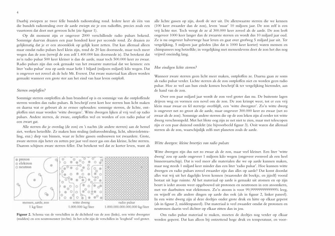
Fig. 2. Example of the fitting of the subpulses.Left panel: stacked pulses in the on-pulse re-gion. Right panel: after finding nulls (lightercolour), and fitting subpulses (crosses at thebase of the fitted Gaussians), we fit the drift-bands (black lines). In this and all other fig-ures, 0◦ longitude is defined as the centre ofthe best Gaussian fit to the average profile.

the strong subpulses and then using their driftpath to suggest the position of weakersubpulses. This approach worked very well.

For our fitting, we assumed the subpulses to be Gaussian in shape, non overlap-ping, and to have a full width at half maximum (FWHM) less than 15◦. We used aLevenberg-Marquadt method (Press et al. 1992) with multiple starting configurationsto produce goodness-of-fit values for different numbers of subpulses. By comparingthese χ2 values, we located the subpulses that had high significance levels.

Upon finding these normal to strong subpulses, we set out to detect the weakerones over the noise. For this purpose we composed driftbands out of the individualsubpulses already identified. On a one-by-one basis, a subpulse was either added to apath that had predicted its position to within P2/4 (P2 being the average separationbetween two subpulses within a single pulse, about 11◦ longitude), or taken to be thestart of a new path. Paths ended if no subpulse fitted the path for more than 5 pulses, orupon reaching a null. On the first run, only paths longer than ten pulses were allowedto survive, so as to eliminate the interference of short run-away paths. This allowed a

18

Fig. 3. Horizontal residuals to straight line fits to the driftbands, individual and binned, for2000 pulses.

steady pattern of long paths to grow, incorporating about 90% of the subpulses found.On the second run, paths longer than 5 pulses were allowed to form: these shorterpaths occur only around nulls, where the normal, long paths are interrupted.

The drifting pattern thus formed predicted the locations of the weaker subpulses.Around each predicted position, we isolated a section of the data. This section wastaken as large as possible without interfering with other, previously fitted subpulses.We checked the significance of fitting a single Gaussian to indicate the presence of asubpulse. In the same way as described above, the final driftpattern was then identifiedusing the extended set of subpulses. To check the method, we compared the observedaverage profile with the one recreated from the Gaussians fits to the subpulses. Fromtheir match, we concluded that the fitting procedure was effective.

3. Results

Driftband fitting

The driftbands are not straight, but show a systematic curvature (Davies et al. 1984).This is seen most strikingly when we plot the residuals to straight line fits: Figure3 shows the longitudinal offset between the actual and predicted positions of thesubpulses. Near the edges of the profile the subpulses arrive later than is to be expectedbased on a linear driftband, in the middle they arrive sooner.

This probably explains the results of Popov & Smirnova (1982). After fittingstraight lines to all driftbands, they find that the driftrate of the last driftband be-fore the null is 20% higher than that of a normal driftband. As seen in the curvature

of the driftbands, however, a normal driftband consists of a fast drifting first half anda slow drifting second half. If a driftband is cut by a null, the part before the nullconsists only of the fast drifting first half, resulting in a higher average driftrate overthis shorter driftband.

To make our results independent of the longitude, the non-linearity of the drift-bands is taken into account in all the following driftrate calculations. In these cases, thepositions of individual subpulses are corrected by subtracting the appropriate residualvalue.

Shortest nulls

The main criterion used to decide whether or not to include certain datasets was thecomplete separation of the on-pulse and off-pulse energy distributions. Therefore,the set of null identified is genuine and complete. This allows us to investigate theunderlying statistics of null occurrence and length, and estimate the influence of shortnulls.

The chance of finding PSR B0809+74 in the null state is on average about 1.4%.If the null lengths were distributed in a Poissonian fashion, we would find a prepon-derance of one-pulse nulls and very few longer ones. However, in the null-lengthhistogram (Fig. 4) we find a peak at nulls of length 2, a significant decrease towardsshorter lengths and a considerable number of long nulls, showing that the occurrenceof nulls is not governed by pure chance.

Comparing this histogram with the one previously found by Lyne & Ashworth(1983), we see that we identify about twice as many one-pulse nulls in the data. Still,many nulls shorter than one period must pass unnoticed, as they occur when the

Fig. 4. Length histogram for the 180 nulls.

19

pulsar faces away from us. We know that nulls, especially long ones, have a distinctimpact on the drifting pattern in their vicinity. Although the impact of shorter nullsis less, a large number of unnoticeable, short nulls (<P1) might seriously influence thedrifting pattern we are trying to understand.

Using the null-length histogram we can estimate the number of these short nulls.It peaks at two-pulse nulls, and the distribution decreases towards shorter lengths.Assuming that the underlying distribution of null-lengths is continuous, this tendencyof decreasing occurrence towards shorter nulls implies that there is a small number ofnulls shorter than one pulse period. Extrapolating the decrease leads to an estimateof about 15 unnoticeable short nulls in the null-length interval from 0 to 0.5 pulses.The low frequency of their occurrence (0.04%) indicates the influence of short nullson the drifting pattern is negligible.

Null versus burst length

The next question we address involves the interval between adjacent nulls (the so-called burst) and the duration of the nulls. Does waiting longer for a null mean it willlast longer, too? We have checked these relationships and have found that the lengthsof neighbouring nulls and bursts are independent.

Position jump over nulls

If the nulling mechanism is independent of the position of the subpulses, we expectthat the distribution of subpulse positions is the same for the normal pulses and thepulses that immediately precede a null. We find no proof of differences in these distri-butions and conclude that there is no preference for a null to start at a certain subpulseposition.

The positions of subpulses change over a null. We derived this shift of the sub-pulse pattern for each null in our sample. As the positions of the individual subpulseswere already identified, this shift was simply extracted. Each subpulse before the nullmatched a subpulse after the null, if the latter fell within −3P2/4 to P2/4 of the for-mer. This range is symmetric around the average expected jump over a null, so asto minimise the number of ambiguous cases. In the following analysis, we used theaverage of all individual subpulse shifts within one pulse.

Figure 5 shows this shift in the subpulse position over a null, corrected for the non-linear behaviour of the driftband. If the motion of the subpulses were independent ofthe emission, the subpulses would continue to drift invisibly throughout the null state,and reappear at a very different position. The associated shift in positions would thenbe spread around the diagonal dashed line in Fig. 5. If, on the other hand, the subpulsedrift would cease abruptly and completely during the null, the jump in position wouldbe between zero and two times the average shift in longitude between normal pulses.The uncertainty in this estimate arises from the fact that neither the start nor end of

the null are known more accurately than to one pulse period. The mean jump inposition over the null would then follow the horizontal dash-dotted line in Fig. 5.

After discarding the three ambiguous cases (points near the top edge of Fig. 5), wecomputed averages for each null length. These averages follow neither of the two casesoutlined above. There is too much change in position over the null to be accountedfor by just an abrupt stop of the drift, and there is no evidence for steady (albeit slowerthan regular) drift during the null. We do see that for nulls longer than one, the jumpis constant, 1.47±0.16◦ above the offset value that we would expect in the case of nodrift. This independence of null length and subpulse jump over the null is shown asthe dotted horizontal line in Fig. 5.

Driftrate around the null

We have computed the driftband slope around nulls, correcting for their general cur-vature.

For the driftrate before the null, we fitted straight lines to the last six subpulses ofeach driftband the ended with the null. We find that this driftrate just before a nulldoes not deviate from the normal driftrate.

The driftrate after nulls is different from the normal driftrate, though. Althoughthere is some spread, all the driftrates we find after longer nulls are lower than thenormal average value (Fig. 6).

Fig. 5. Jump in subpulse position against null length. The bottom of the plot falls at P2/4, thetop at −3P2/4. The diagonal dashed line is the predicted subpulse path if the drifting wereindependent of the nulls. The horizontal dash-dotted line is the predicted path for a suddenand complete stop of drifting during the null. The horizontal dotted line is the average jumpfound for the nulls longer than 1 period.

20

Fig. 6. Drift after the null versus the length of the null. We show the average driftrate ofthe first 6 pulses for each driftband after a null (gray points). The average per null length (blackpoints) with its error is also plotted. The normal driftrate, corrected for the driftband curvature,is indicated by the horizontal dashed line. The stars denote the driftrate for the slow driftingmode sequences. One pulse often consists of more than one subpulse, so after many nulls wesee several driftbands reappear. The number of driftrates plotted here is therefore larger thanthe total number of nulls.

Average pulse profile around null

To investigate whether the change from normal emission to the null state is suddenor more gradual, Lyne & Ashworth (1983) compared the energies of the pulses neara null. The finite chance that the emission from the pulsars drops or rises within thepulse window would influence the brightness of the pulses around the null. The lastpulse before the null was indeed found to be less bright than a normal pulse. The firstpulse after the null, however, was considerably more bright than a normal pulse.

We have not just looked at the energies of these neighbouring pulses, but also attheir profiles. To this end, we have averaged all the last pulses before nulls longer than1 period, and all the first pulses after these nulls. The results, shown in Fig. 7 andcondensed in Table 1, are surprising. Not only do we find the expected differences inbrightness, we also see a significant offset in the pulse position for the first pulses afternulls.

Slow drifting mode

Although we had set out to quantify the normally very regular drifting behaviour ofPSR B0809+74, we unexpectedly found two occasions in which the pulsar clearlydeviates from its normal drifting mode. We will refer to these sequences by the year

in which they were observed, 1999 and 2000. In Fig. 8a we have plotted the derivedlongitude (Lyne & Ashworth 1983) of subsequent pulses around the mode changes.The derived longitude of the subpulses effectively converts the different short drift-bands into one long one. Figure 9 shows a grayscale plot of the two slow driftingseries.

The most striking difference, as the drifting pattern is concerned, is clearly thedecrease of the driftrate by about 50%. We see that in both the observations thedrifting mode changes during or immediately following a long null. After these nullsof length 10 and 5 respectively, almost all drifting properties reappear at new values,as laid out in Table 2. As some of these properties normally already show change overtime, we compare the slow drifting sequences (labeled ‘slow’) to the 600 pulses thatsurround them (labeled ‘normal’).

In the first three columns of Table 2, we investigate the parameters of the in-dividual subpulses in both modes. Immediately we see a very interesting change inthe relative average position of the subpulses. Right after the null, there is a definiteshift in position towards earlier arrival, that can already be seen in a plot like Fig. 9.Interestingly, this shift of the pulse window is similar to the average jump in subpulseposition we see over a normal null.

In the slow drifting mode, the subpulses are slightly wider, but their heights remainthe same. Next, we explore the driftband characteristics in the last three columns ofTable 2. The average longitude separation of two adjacent driftbands, P2, decreasessignificantly by about 15%. Hence, in the slow drifting mode the subpulses withineach pulse are spaced closer together than normal.

Fig. 7. Average profiles for the pulses adjacent to nulls, for all 131 nulls longer than 1 pulse.Shown are: the first active pulse after the null, the last active pulse before the null and, forreference, the normal average profile.

21

Fig. 8. a) Derived longitudes of three pulse sequences. The gaps in the curves are nulls. Thesequences are aligned on the ends of the long nulls around pulse 200. The top line shows thenormal drifting behaviour around nulls of lengths 13, 9, 3 and 2, respectively. The middle lineshows the 1999 slow drifting sequence (offset −150◦), the bottom line shows the 2000 sequence(offset −300◦). b) Deviation of the derived longitude from normal drifting for the 1999 andthe normal sequence shown in panel (a). The transitions from slow to normal drifting havebeen aligned.

When we compare the driftrates of the subpulses between the two modes, wefind that the driftrate in the slow drifting mode is almost halved. This puts the newdriftrate right in the range of driftrates we usually find after a longer null. We haveindicated these driftrate values with black stars in Fig. 6. Being dependent on P2

and the driftrate, the fractional change in P3 (the recurrence time of a driftband) iscomparably large.

In both cases the new drifting mode is stable for about 120 pulses and then changesback to normal. To illustrate this change, we have plotted the deviation of the derivedlongitude from normal drifting in Fig. 8b. For the 1999 observation, we see a normal

driftrate up to the null at pulse 200. After this null, the driftrate is smaller, up to pulse330. In about 20 pulses, the drift then speeds up back to its normal value.

For reference, we have also plotted the drifting behaviour after the longest nullin our sample. Again, we see a speedup to the normal driftrate in about 20 pulses atpulse 330, very similar to the slow drifting speedup time scale.

The slow drifting interval in the 2000 observation (right panel of Fig. 9) is fol-lowed and stopped by a series of frequent, longer than average nulls, out of which thepulsar emerges in its normal drifting pattern.

These surprising changes in subpulse positions, widths and separations must influ-ence the average pulse profile during the slow drifting mode. Noting the many simi-larities between slow drifting pulses and the pulses that follow nulls (halved driftrate,similar offsets, similar speedup) we are interested in the possible similarities betweenthe average profiles of these pulses, especially since the average profile of the pulsesafter the null is singularly bright and shifted in longitude.

In Fig. 10 and Table 1 we compare the pulsar’s normal average profile with theaverage profile in the slow drifting mode. In both observations, the slow driftingmode average profile is much brighter than the normal profile and offset towardsearlier arrival – exactly the two peculiarities we found in the average pulse profileafter a null as well.

4. Discussion

Driftband fitting

We find that the number of invisible nulls is low. That means we can study of thedrifting properties of PSR B0809+74 straightforwardly.

height position (◦) fwhm (◦)normal 1.000 ± 0.003 0.000 ± 0.016 13.33 ± 0.04last active 0.875 ± 0.005 0.27 ± 0.12 13.96 ± 0.09first active 1.112 ± 0.005 −0.77 ± 0.12 13.84 ± 0.08slow 1999 1.272 ± 0.005 −1.51 ± 0.3 11.99 ± 0.06slow 2000 1.311 ± 0.008 −0.75 ± 0.3 10.52 ± 0.08

Table 1. Comparison of the pulsar’s average emission profiles for different sets of pulses. Weshow the height, full width at half maximum (fwhm) and position of the Gaussians that fittedthe profiles best. The ‘normal’ subset consist of all non-null pulses in the dataset. All heights andpositions in this table are relative to the height and position of this ‘normal’ set. The set labeled‘last active’ contains all 131 pulses that preceded a null that was longer than 1 pulse period. Thecharacteristics of the pulses that followed these nulls are labeled ‘first active’. The subsets ‘slow1999’ and ‘slow 2000’ contain the 120 pulses that form the slow drifting sequences observed in1999 and 2000, respectively.

22

Fig. 9. Grayscale plots of the pulses composing the two slow drifting sequences. The grayscalelinearly depicts the intensity of a sample. The left series was observed in 1999, the right seriesin 2000. After a null of length 10 (1999 series) and 5 (2000 series) around pulse number 100,the driftrate and driftband separation are steadily different for about 120 pulses. From pulse 240on, the drifting changes back to normal.

The non-linearity of the driftbands was already noted by Page (1973), who inte-grated several hundreds of pulses to compare the shape of the driftbands in differentobservations. He found considerable differences between these driftband shapes. We

compare the average drift path over several thousands of pulses however, and find thatthe curvature of the driftbands remains the same.

The curvature of the driftband can be a direct consequence of the curved ge-ometry of the emission region (Krishnamohan 1980). In that case, the shape of thedriftband is expected to be point-symmetric: the curve will then be unchanged aftermirroring it in both axes. This point-symmetry would then return in the residuals tostraight line fits (Fig. 3). The shape of the driftbands we find, however, is not point-symmetric but axisymmetric: the curve is unchanged after mirroring in the y-axis.

We could still tie the curvature of the driftbands to the emission-region geometry,by assuming that part of the pulse profile of this pulsar is missing. In that case, thedriftband shape we find would represent only part of the total expected shape. Thissuggestion that part of the profile of PSR B0809+74 is missing fits in with multi-frequency observations (Bartel et al. 1981; Kuzmin et al. 1998) that imply ‘absorption’of part of the profile at lower frequencies.

Slow drifting mode and nulling

With our investigation of PSR B0809+74 still ongoing, we discuss here only thephenomena themselves and defer their interpretation to a subsequent paper.

The similarity between this pulsar’s behaviour in the slow drifting mode andaround nulls is striking:

– The slow drifting sequences start at nulls.– The driftrate of the slow drifting mode is a lower limit to the driftrates found after

all nulls.– The speedup from slow drifting to normal is identical to the speedup after a null.– The average profiles of both the post-null and slow drifting pulses are brighter

than normal.– These average profiles are both displaced to earlier arrival.– This displacement of the average profile is caused by offsets in the individual

subpulses.– These offsets are identical to the jump of the subpulses over the null.

The natural conclusion is that the behaviour after a null and the slow driftingmode are the same, quasi-stable phenomenon. Normally the pulsar reappears fromthe null in the slow drifting mode. After a variable time, it quickly evolves to thenormal mode. Therefore, right after a normal null we see either a short sequence ofslow drifting, or the transition back to normal drifting. In the case of the long slowdrifting mode sequences, the metamorphosis back to the normal mode is delayed.

This would explain all the similarities we found above. After a normal null, thepulsar is in the slow drifting mode or changing back to the normal mode. All thecharacteristics of the slow drifting mode can then be identified in the post-null be-haviour, although they will be less pronounced; the transition to normal drifting mayalready be taking place.

23

Table 2. Subpulse and driftband properties for the slowdrifting mode sequences and the surrounding normal drift-ing pattern.

averages from Gaussian fits to subpulses averages from straight line fits to driftbandsrelative height relative position (◦) fwhm (◦) P2 (◦) driftrate (◦/P1) P3 (P1)

normal 1999 1.00 ± 0.02 0.00 ± 0.11 5.39 ± 0.06 11.61 ± 0.14 1.086 ± 0.011 10.72 ± 0.13slow 1999 1.06 ± 0.05 −1.2 ± 0.3 5.75 ± 0.11 9.9 ± 0.5 0.606 ± 0.019 16.5 ± 0.5

normal 2000 1.00 ± 0.02 0.0 ± 0.2 5.22 ± 0.06 11.33 ± 0.14 1.043 ± 0.014 10.88 ± 0.13slow 2000 0.99 ± 0.04 −1.8 ± 0.2 5.55 ± 0.11 9.63 ± 0.3 0.54 ± 0.02 17.6 ± 0.5

When the driftrate increases at the end of a slow drifting sequence, this speedupis quick and identical to the speedup seen after a normal null (see Fig. 8b).

The post-null driftrate values are found in between the slow drifting and normaldriftrate value, depending on how soon the transition back to normal takes place (seeFig. 6). Although the return from the low to the normal driftrate will be quick, thetime the driftrate is low may vary for different nulls of the same length. The averageof these different sequences will then resemble the slow exponential decay found byLyne & Ashworth (1983).

Comparing average pulse profiles, the increased brightness and the pulse offset ofthe post-null average profile are attenuated versions of similar deviations seen in theslow drifting mode profile (see Table 1, Figs. 7 and 10). The average profile offsetwe see in the slow drifting mode is caused by a shift of the window in which thesubpulses appear (Tables 2 and 1).

The change in position of the post-null average pulse profile must then be causedby this shift of the pulse window as well. The magnitude of this shift is identical tothe subpulse-longitude jump over normal nulls. This means that the subpulse-positionjump over a null is caused by a displacement of the pulse window as a whole, like inthe slow drifting mode.

Previously, this jump was thought to be the effect of the subpulse-drift speedupduring the null. For this speedup to produce the observed jump in subpulse position,the time scale involved had to be long, contrasting the short time scales found for theslowdown of the subpulse drift and the rise and fall of the emission around a null.

With the displacement of the subpulses over the null accounted for, the estimatedspeedup time of the subpulse drifting is negligible: the preservation of the position ofthe subpulses over the null now only allows for a quick speedup of the subpulse drift,putting all time scales of emission and drift rise and decay around the nulls in the samerange.

5. Conclusions

After many or all nulls, PSR B0809+74 emits in a mode different from the normalone. This mode is quasi-stable, normally changing back to normal in several pulses.This is seen as the normal behaviour after a null, of which the reduced driftrate is themost striking characteristic. Occasionally, the quasi-stable slow drifting configurationpersists for over a hundred pulses before changing back to the normal mode.

The pulses in the slow drifting mode and, consequently, all pulses after the null,are brighter than normal pulses. In the slow drifting mode, the subpulses are closertogether, they drift more slowly through the profile and the window in which theyappear is offset towards earlier arrival.

This offset of the pulse window accounts for the displacement of subpulses overthe null. When taking this shift of the window into account, we find that the longi-tude of the subpulses is perfectly conserved over a null. This indicates that the speeduptime for the subpulse drift is short.

Fig. 10. Average profiles for the slow drifting mode sequences. The ‘slow 1999’ and ‘slow 2000’profiles are averaged over the 120 pulses that composed the slow drifting sequences observed in1999 and 2000, respectively. The normal average profile is plotted for comparison.

Chapter 2

PROBING DRIFTING AND NULLING MECHANISMSPROBING DRIFTING AND NULLING MECHANISMSTHROUGH THEIR INTERACTION IN PSR B0809+74THROUGH THEIR INTERACTION IN PSR B0809+74

with Ben Stappers, Ramachandran and Joanna RankinBoth nulling and subpulse drifting are poorly understood phenomena. We probe their mechanisms by investigating how they interact in PSR B0809+74. We find that the subpulse drift is not aliased but directly reflects the actual motion of the subbeams. The carousel-rotation time must then be over 200 seconds, which is much longer than theoretically predicted. The drift pattern after nulls differs from the normal one, and using the absence of aliasing we determine the underlying changes in the subbeam-carousel geometry. We show that after nulls, the subbeam carousel is smaller, suggesting that we look deeper in the pulsar magnetosphere than we do normally. The many strikingsimilarities with emission at higher frequencies, thought to be emitted lower too, confirm this. The emission-height change as well as the striking increase in carousel-rotation time can be explained by a post-null decrease in the polar gap height. This offers a glimpse of the circumstances needed to make the pulsar turn off so dramatically.

27

1. Introduction

In pulsars, the emission in individual pulses generally consists of one or more peaks(‘subpulses’), that are much narrower than the average profile and the brightness,width, position and number of these subpulses often vary from pulse to pulse.

In contrast, the subpulses in PSR B0809+74 have remarkably steady widths andheights and form a regular pattern (see Fig. 1a). They appear to drift through the pulsewindow at a rate of −0.09 P2/P1, where P2 is the average longitudinal separation oftwo subpulses within one rotational period P1, which is 1.29 seconds. Figure 1a alsoshows how the pulsar occasionally stops emitting, during a so-called null.

In this paper, we will interpret the drifting subpulse phenomenon in the rotatingcarousel model (Ruderman & Sutherland 1975). In this model, the pulsar emissionoriginates in discrete locations (‘subbeams’) positioned on a circle around the magneticpole. The circle rotates as a whole, similar to a carousel, and is grazed by our line ofsight. In between successive pulses, the carousel rotation moves the subbeams throughthis sight line, causing the subpulses to drift.

Generally, the average profiles of different pulsars evolve with frequency in a sim-ilar manner: the profile is narrow at high frequencies and broadens towards lowerfrequencies, occasionally splitting into a two-peaked profile (Kuzmin et al. 1998).This is usually interpreted in terms of ‘radius to frequency mapping’, where the highfrequencies are emitted low in the pulsar magnetosphere. Lower frequencies originatehigher, and as the dipolar magnetic field diverges the emission region grows, causingthe average profile to widen.

The profile evolution seen in PSR B0809+74 is different. The movement of thetrailing edge broadens the profile as expected, but the leading edge does the opposite.The profile as a whole decreases in width as we go to lower frequencies until about 400MHz. Towards even lower frequencies the profile then broadens somewhat (Davieset al. 1984; Kuzmin et al. 1998). Our own recent observations of PSR B0809+74,simultaneously at 382, 1380 and 4880 MHz, confirm these results (Rankin et al.2002). Why the leading part of the expected profile at 400 MHz is absent is not clear.While Bartel et al. (1981) suggest cyclotron absorption, Davies et al. (1984) concludethat the phenomenon is caused by a non-dipolar field configuration. We will referto this non-standard profile evolution as ‘absorption’, but none of the arguments wepresent in this paper depends on the exact mechanism involved.

In Chapter 1 (van Leeuwen et al. 2002) we investigated the behaviour of thesubpulse drift in general, with special attention to the effect of nulls. We found thatafter nulls the driftrate is less, the subpulses are wider but more closely spaced, andthe average pulse profile moves towards earlier arrival. Occasionally this post-null driftpattern remains stable for more than 150 seconds.

For a more complete introduction to previous work on PSR B0809+74, as wellas for information on the observational parameters and the reduction methods used,we refer the reader to Chapter 1. In this paper we will investigate the processes thatunderly the post-null pattern changes. We will quantify some of the timescales asso-

Fig. 1. Observed and fitted pulse sequences. A window on the pulsar emission is shown for150 pulses. One pulse period is 360◦. The centre of the Gaussian that fits the pulse profile bestis at 0◦. a) The observed pulse sequence, with a null after pulse 30. b) The Gaussian curvesthat fitted the subpulses best. Nulls are shown in lightest gray, driftbands fitted to the subpulsepattern are medium gray.

ciated with the rotating carousel model and map the post-null changes in the driftpattern onto the emission region.

28

One of the interesting timescales is the time it takes one subbeam to complete arotation around the magnetic pole. This carousel-rotation time is predicted to be ofthe order of several seconds in the Ruderman & Sutherland model. Only recently acarousel-rotation time was first measured: Deshpande & Rankin (1999) find a peri-odicity associated with a 41-second carousel-rotation time for PSR B0943+10.

The second goal is to determine the changes in the emission region that underlythe different drift pattern we see after nulls. Mapping this emission region couldincrease our insight into what physically happens around nulls.

Achieving either goal requires solving the so-called aliasing problem: as the sub-pulses are indistinguishable and as we observe their positions only once every pulseperiod, we cannot determine their actual speed.

2. Solving the aliasing problem

The main obstacles in the aliasing problem are the under sampling of the subpulsemotion and our inability to distinguish between subpulses. The pulsar rotation onlypermits an observation of the subpulse positions once every pulse period. Followingthem through subsequent pulses might still have led to a determination of their realspeed, but unfortunately the subpulses are so much alike that a specific subpulse inone pulse cannot be identified in the next, making it impossible to learn its real speed.

In Fig. 2 we show a simulation of subpulse drifting, where we have marked allsubpulses formed by a particular subbeam with a darker colour. We use these simu-lations to discuss how the driftrate, which is the observable motion of the subpulsesthrough subsequent pulses, is related to the subbeam speed, which cannot be deter-mined directly. In Fig. 2a the speed of the subbeams is low (−0.09 P2/P1) and identicalto the driftrate. In Fig. 2b the subbeam speed is higher (0.91 P2/P1), but the drift-rate is identical to the one seen in Fig. 2a. When the differences between subpulsesformed by various subbeams are smaller than the fluctuations in subpulses from onesingle subbeam, these two patterns cannot be distinguished from one another. In thatcase the subpulses within one driftband, which seem to be formed by one subbeam,can actually be formed by a different subbeam each pulse period (‘aliasing’).

To solve the aliasing problem for PSR B0809+74 we follow driftrate changes afternulls to determine the subbeam speed. Nulls last between 1 and 15 pulse periods, andin Chapter 1 we have shown that for each null the positions of the subpulses beforeand after the null are identical if we correct for the shift of the pulse profile. So, asthere is no apparent shift in subpulse position, either the subbeams have not moved atall, or their movement caused the new subpulses to appear exactly at the positions ofthe old ones.

As the lengths of the nulls are drawn from a continuous sample it is highly unlikelythat the subbeam displacement is always an exact multiple of the subpulse separation:only a total stop of the subbeam carousel can explain why the subpulse positions arealways unchanged over the null. At some point after the null, however, the subbeams

Fig. 2. Different alias orders illustrated. We show two series of stacked simulated drifting sub-pulses. We have marked the subpulses formed by one particular subbeam with a darker colour.a) At a low subbeam speed, a single subbeam traces an entire driftband by itself. The driftrate isidentical to the subbeam speed: alias order 0. b) At alias order −1, the subbeam speed is higherthan the driftrate and in opposite direction.

have accelerated, and the drift pattern has returned to normal. In Fig. 1 we see how,after a null, the driftrate increases to its normal value in about 50 pulses.

There are two scenarios for this subbeam acceleration. The first we will call grad-ual speedup. Here the changes in the subbeam speed occur on timescales larger thanP1. The second we will call instantaneous, as the entire acceleration happens within1P1, effectively out of sight.

In Fig. 3 we show four simulated pulse sequences with different speedup param-eters. In all cases, we simulate a drift pattern like that of PSR B0809+74. During anull, from pulses 30 to 45, there is no subbeam displacement. Immediately after thenull the subbeams build up speed, and each pulse period we translate the subbeam

29

displacement to a change in subpulse position. Although the final driftrate is the samefor all scenarios (−0.09 P2/P1), the subbeam speeds differ considerably. The bottomfour graphs show these speeds for each scenario. In the top four diagrams we havemarked the subpulses from one subbeam with a darker colour for clarification.

Let us look at the case of gradual speedup to alias order 0, where the subbeamspeed is the same as the driftrate (Fig. 3a). In this case the driftrate will graduallyincrease and form a regular driftband pattern, much like the pattern found in theobservations.

Next, we investigate a subbeam acceleration to a slightly higher speed. At 0.91P2/P1, Fig. 3b shows alias mode −1, which is the simplest configuration in whichthe subbeams move opposite to the subpulse drift. Right after the null the drift con-sequently commences in this opposite direction. When the subbeam speed nears thefirst aliasing boundary 0.5 P2/P1, the subpulses seem to move erratically through thewindow. After the subbeam speed passes the first alias boundary, the subpulse driftresumes its normal direction, and as the subbeam speed approaches 0.91 P2/P1, thedrift pattern returns to normal.

Also in the ‘alias order 1’ scenario (Fig. 3c), which is the simplest aliased modein which the subbeams move in the same direction as the subpulses, the subpulseswander when the subbeam speed nears an alias boundary. Such a disturbance of thedrift pattern turns out to be present in all simulations of non-zero alias orders. Becausethe observed pulse sequences always show smooth, non-wandering driftbands (like inFig. 1a), we conclude that the subbeams cannot accelerate gradually to a high speed.

With instantaneous acceleration the subbeam speed switches suddenly. Most likelyit will do so when the pulsar beam faces away from us. After we see pulse number n,the subbeams will move slowly for a certain time, quickly speed up, and then movefast until we see the subpulses of pulse n + 1 appear. The actual speedup can occurany moment between seeing pulses n and n + 1. This means that the displacementof the subbeams can vary from very little (speedup just before pulse n + 1) to a lot(speedup right after pulse n). The accompanying changes in subpulse position willthen be evenly distributed between 0 and P2; the subpulse positions after the speedupwill not be related to those before.

If the subbeams accelerate instantaneously at the end of a null, before the firstpulse can be observed, the subpulse phases are not preserved over the null. As this isopposite to what is observed, this possibility is ruled out.

If the subbeam acceleration occurs a few pulses after a null, we expect that thechange in driftrate will nearly always be accompanied by a sudden change in thelongitude of the driftband, as illustrated in Fig. 3d for a final subbeam speed of −1.09P2/P1. The absence of a significant number of such sudden shifts in the data indicatesthat the subbeam carousel of PSR B0809+74 does not speed up instantaneously to ahigh speed.

As only the gradual speedup to alias order 0 can explain the observed drift patterns,the drift seen in the subpulses of PSR B0809+74 directly reflects the movement ofthe subbeams, without any aliasing.

3. Discussion

Alias order of other pulsars

The subbeam speedup in PSR B0809+74 follows the simplest scenario possible: it isgradual, and the subpulse drift is not aliased. In other pulsars this might not be thecase, and for those we predict drift-direction reversals or jumps in driftband longitudeduring the subpulse-drift speedup phase after nulls.

Subbeam-carousel rotation time

Having resolved the aliasing of the subpulses’ representation of the subbeams, weknow that the subbeams move at −0.09 P2/P1. Such a low rotation rate means itwill take each subbeam 11P1 to move to the current position of its neighbour. Thefollowing estimate of the number of subbeams then leads directly to the carousel-rotation time.

Towards the edges of the profile the sight line and the carousel move away fromeach other, and a subbeam will cease to be visible when the sight line no longercrosses it. When the subbeams are small, or widely spaced compared to the curvatureof the carousel, the sight line will cross only few. In that case there will not be manysubpulses visible in one pulse. If, however, the subbeams are large and closely spacedcompared to the carousel curvature, the sight line passes over more subbeams in onetraverse, leading to many subpulses per pulse.

In most of the pulses of PSR B0809+74 we observe two subpulses, occasionallywe discern three. By combining this with the ratio of the subpulse width and separa-tion we find there must be more than 15 subbeams on the carousel. As one subbeamreaches the position of its neighbour in 11P1, a 15-subbeam carousel rotates in over200 seconds.

Persistent differences in the properties of individual subbeams should introduce along term periodicity in the pulse sequences, at the carousel-rotation frequency. Thusfar, no such periodicity has been found, which is not surprising as the periodicitycan only be measured if the lifetime of the subbeam characteristics is longer than thecarousel-rotation time.

In PSR B0943+10, the only pulsar for which we know how the subbeams vary(Deshpande & Rankin 1999, 2001), the associated timescales are in the order of 100seconds. If we assume their lifetimes are comparably long in PSR B0809+74, thesubbeams will have lost most of their recognisable traits once they return into viewafter one carousel rotation. Having regular pulse sequences that contain several tensof rotation times might still show some periodicity at the carousel-rotation frequency.

30

Fig. 3. Simulated scenarios for subbeamspeedup. The top panels show the result-ing drift patterns. Nulls are shown in light-est gray, driftbands fitted to the subpulse pat-tern are overdrawn in medium gray. We havemarked the subpulses formed by one partic-ular subbeam with a darker colour. The bot-tom panels show the subbeam speed versusthe pulse number. a) Gradual acceleration toa subbeam speed equal to the driftrate (aliasorder 0). b) Gradual acceleration to a sub-beam speed larger than the driftrate and inopposite direction (alias order -1) c) Gradualacceleration to a subbeam speed larger thanthe driftrate and in the same direction (aliasorder 1) d) Instantaneous acceleration, againto alias order 1.

Unfortunately nulls have a destructive influence on the driftband pattern and possiblyon the subpulse characteristics. This has thus far made it impossible to observe brightsequences longer than 3 times our lower limit on the rotation time of 200 seconds.

After the prediction that the rotation time in most pulsars would be on the or-der of several seconds (Ruderman & Sutherland 1975), the observation that it is 41

seconds in PSR B0943+10 was somewhat surprising. The suggested dependence ofthe carousel-rotation time on the magnetic field strength and the pulse period pre-dicts that the rotation time in PSR B0809+74 should be roughly 4 times smaller. Thecirculation time we observe, several hundreds of seconds, shows that the theoretical

31

Fig. 4. Pulse profiles for the normal mode and the two longest slow drifting sequences afternulls described in Chapter 1. The broadening of the subpulses causes the slow-drifting profileto outshine the normal one. Here all three profiles have been scaled to the same height to showthe change in the pulse location and shape.

predictions are incorrect in absolute numbers as well as in the scaling relations theypropose.

Emission region geometry

In Chapter 1 we found many interesting changes in the driftband pattern after nulls.The subpulses reappear 5−10% broader and 15% closer together, which results in abrighter average profile. The individual subpulses move 1.5◦ towards earlier arrival, asdoes their envelope, the average profile, with 1.1◦ (Fig. 4). The subpulses drift 50%more slowly than usual. Occasionally, this slow drifting pattern remained stable forover 100 pulses.

Knowing, as we do now, that there is no aliasing involved, we can identify singlesubpulses with individual subbeams. This implies that we can interpret the drift pat-tern changes in terms of the subbeam-carousel geometry (Fig. 5). We will do so foreach of the altered characteristics.

The first thing we note is that, relative to the shift of the average profile, thepositions of the subpulses are unchanged over nulls. This means that the subbeamcarousel has not rotated during the null.

After nulls, the subpulses are positioned about 15% closer together. In principle,this could be the result from a change in subbeam speed. At a certain moment, aparticular subbeam will be pointing towards the observer. It takes some time beforethe pulsar has rotated the next subbeam into the observer’s view, and during this time

the subbeams themselves have moved, too. This motion translates directly to a changein the longitudinal subpulse separation. Yet, as we have shown that subbeam speed islow, this effect is negligible.

A more significant change in P2 could be caused by an increase in the number ofsubbeams on a carousel of unchanged size. The other option is that a decrease in thecarousel radius moves the subbeams closer together.

In the first scenario the number of subbeams would have to change during thenull, causing the subbeam placement to change considerably. This would lead tosubpulse-position jumps over the null. In that case, we would not expect the phasesof the subpulses to be as unchanged over the nulls as is observed. Secondly, some timeafter the null the new configuration would have to return to normal. This meanssubbeams would have to appear or disappear. We see no evidence of this in any of the200 nulls we observed. The change in the subbeam separation P2 can therefore notbe due to a changed number of subbeams.

In the second scenario the carousel radius decreases by 15%, but the number ofsubbeams remains the same. As the subbeams now share a reduced circumference,their separation also decreases.

The contraction of a carousel causes all subpulses to move towards the longitudeof the magnetic axis. If we combine this contraction with the aforementioned absorp-tion, we can immediately explain the observed shift to earlier arrival of the subpulsesand their envelope, the average profile: with only the trailing part unabsorbed, allvisible subpulses move towards earlier arrival (Figs. 4 and 5).

In general, the subpulses farthest from the longitude of the magnetic axis willmove most, while those at it, if visible, will remain at their original positions.Enlargement of our sample of subpulse positions can therefore indicate were the mag-netic axis of PSR B0809+74 is located. This would immediately indicate how muchof the pulse profile is ‘absorbed’ and illuminate the thus far much debated alignmentof the pulse profiles at different frequencies.

Normally, the edges of a pulse profile indicate where the overlap of the sight lineand the subbeam carousel begins and ends. The contraction of a carousel will thenmove both edges inward. Yet when the first part of the profile is absorbed, the leadingedge reflects the end of the absorption. If this edge is near the middle of the sight-linetraverse over the carousel, it will not be affected by a reduction of the carousel size.In that case we will see a change in the position of the trailing edge but not in theleading one, which is exactly what we observe in PSR B0809+74 (Fig. 4).

The wider subpulses we see after a null translate directly to wider subbeams. Wedo note that a change in carousel radius leads to a new sight-line path, which mayhave an impact as well.

The significant chance that a null starts or ends within the pulse window of thepulses that surround it, would on average make these pulses dimmer than normalones (Lyne & Ashworth 1983). Quite unexpectedly however, the pulses after nullswere found to be brighter than average. This is easily explained in our model: the

32

Fig. 5. Subbeam carousel geometry in thenormal and the post-null configuration. a)The normal configuration, with a sight linethat is partially obscured by the absorption.b) After nulls the carousel is smaller. Astheir number is unchanged, the subpulseshave moved closer together. On the non-absorbed, trailing edge, the pulse windowmoves inward. The leading edge of the pro-file is located where the absorption ends anddoes not move. The subpulses are wider andrevolve less fast.

change in the carousel geometry causes the subpulses to broaden and become moreclosely spaced, while their peak brightness remains the same. This leads to the post-null pulse-intensity increase that is observed.

Post-null polar gap height

If we follow the radius-to-frequency-mapping argument discussed in the introduc-tion, then the reduction of the carousel size implies that the emission after a nullcomes from lower in the pulsar magnetosphere than it does normally. The reductionof the subbeam separation supports this idea, but the broadening of the subpulsesseems inconsistent.

At this stage a comparison with the pulse profiles and drift patterns observed athigher frequencies seems promising. Emission at higher frequencies is also supposedto originate lower in the pulsar magnetosphere, so similar effects may point at onecause: a decrease in emission height.

Much like the post-null profile, the average profile at higher frequencies movestowards earlier arrival (Rankin et al. 2002). Comparing drift patterns, we see that athigher frequencies the driftrate decreases and that the subpulses broaden and movecloser to one another (Davies et al. 1984), strikingly similar to the behaviour we findafter nulls.

Only one anomaly remains: when comparing drift patterns at different frequen-cies, the changes in driftrate and subpulse separation P2 always counterbalance, leavingthe carousel rotation time P3 unchanged. This means that the subbeams we observeat a certain frequency are cuts through rods of emission, intersections at the emissionheight associated with that frequency. The rods rotate rigidly but diverge with in-

creasing height. At each height P3 is the same, while the speed and separation of thesubbeams do change.

In contrast to this normal invariance of P3, we see it change considerably afternulls, an increase that cannot be explained by a change in viewing depth. We thereforeexpect that the disturbance that caused the change in this depth, can also account forthe 50% increase in P3.

Usually, both the subbeam separation P2 and the emission height are assumed toscale with the polar gap height h (Ruderman & Sutherland 1975; Melikidze et al.2000). The 15% decrease in P2 would thus be due to a identical fractional decrease inthe gap height, which should also cause an equal decrease in emission height.

If this change in gap height could also account for the observed increase of thecarousel rotation time P3, all post-null drift-pattern changes can be attributed to onesingle cause.

P3 is thought to scale as h−2. For the inferred 15% gap height decrease this predictsa 40% increase in P3, nicely similar to the 50% we find.

With one single cause we can therefore explain both the puzzling well-knownphenomena (the driftrate decrease after nulls, the bright first active pulse) and thenewly discovered subtle ones (the change in the position of the average profile, thedecrease of the subpulse separation and the subpulse-width increase). This post-nulldecrease in gap height offers a glimpse of the circumstances needed to make the pulsarturn off so dramatically.

4. Conclusions

We have shown that the drift of the subpulses directly reflects the actual motion ofthe subbeams, without any aliasing.

33

In other pulsars with drifting subpulses this may be different: for those we predictdrift-direction reversals or longitude jumps in the post-null drift pattern.

We find that the carousel-rotation time for PSR B0809+74 must be long, prob-ably over 200 seconds. The expected lifetime of the subbeam characteristics is less,which explains why thus far no periodicity from the carousel rotation could be foundin the pulse sequence.

The rotation time we find is larger than theoretically predicted, not only in abso-lute numbers but also after extrapolating the rotation time found in PSR B0943+10.Both the magnitude and the scaling relations that link the carousel-rotation time tothe magnetic field and period of the pulsar are therefore incorrect.

When the emission restarts after a null the drift pattern is different, and havingdetermined the alias mode, we identify the underlying changes in the geometry ofthe subbeam carousel. A combination of a decrease in carousel size and ‘absorption’already explains many of the changes seen in the post-null drift pattern.

The resemblance between the drift pattern after nulls and that seen at higherfrequencies, thought to originate at a lower height, is striking. Assuming that similareffects have identical causes leads us to conclude that after nulls we look deeper in thepulsar magnetosphere, too.

Both this decrease in viewing depth and the striking increase in the carousel rota-tion time can be quantitatively explained by a post-null decrease in gap height.

Chapter 3

INTERMITTENT NULLS IN PSR B0818INTERMITTENT NULLS IN PSR B0818-13,AND THE SUBPULSEAND THE SUBPULSE-DRIFT ALIAS MODEDRIFT ALIAS MODE

with Gemma JanssenWe show that all long nulls in PSR B0818-13 are trains of rapidly alternating nulls and pulses (each shorter than one pulse period). Sometimes only the nulls coincide with our pulse window, resulting in one of the apparently long nulls seen occasionally.We show these are seen as often as expected if during such a train the probability for nulls is 1.2 times less than for pulses. During nulls, the subpulse drift-speed appears to increase. We assume that the carousel of sparks that possibly underlies the subpulses actually slows down, as it does in similar pulsars like PSR B0809+74, and conclude that the subpulse-drift in this pulsar must be aliased. The carousel must then rotate in 30 seconds or less, making it the fastest found to date.

37

1. Introduction

Observations of drifting subpulses are a nice example of undersampling: in someradio pulsars the positions of the pulse components change regularly (as in fig. 1), butas these positions are determined only once per pulse period, the exact underlyingmotion remains unknown.

Finding this underlying motion, and its relation to other pulsar parameters, couldbe helpful in determining which, if any, of the proposed mechanisms to generatedrifting subpulses (Ruderman & Sutherland 1975; Wright 2003) is correct. We willassume the subpulses are formed by discrete locations of emission (‘sparks’) that ro-tate around the magnetic pole of the pulsar, causing the pulse components to movethrough the pulse windows (‘drifting subpulses’). Different directions and speeds ofthis rotation can produce identical subpulse positions at the observer, so-called alias-ing (see also fig. 2 in Chapter 2). To determine the actual speed of the spark carousel,one can check for the periodicity caused as brighter or offset sparks re-appear af-ter one carousel rotation. Deshpande & Rankin (1999) did so for PSR B0943+10,and found a carousel rotation time of around 41 seconds, longer than expected fromtheory (Ruderman & Sutherland 1975). With the rotation time known, Deshpande& Rankin (1999) could track individual sparks. They noted that sparks retain theircharacteristic brightness and positions for about 100 seconds. If this number were thesame in other pulsars, carousel rotation times longer than 100 seconds could not befound by a periodicity search, as the characteristic traits of the subpulses will havechanged before they return into view. For such long carousel rotation periods a dif-ferent technique is needed.

In some pulsars there is a mechanism that can be used to circumvent the under-sampling problem and hence determine the underlying carousel-speed: nulling. Inthese pulsars, a few percent of the pulses are missing as the pulsars suddenly turns off(‘nulls’). After these nulls, the subpulse drift is often affected. In Chapter 1 and 2, vanLeeuwen et al.) investigated this drifting-nulling interaction in PSR B0809+74 andfind it can only be explained if the underlying carousel rotates in over 200 seconds,again much longer than expected. They predict that in pulsars with shorter carouselrotation times the drift direction should reverse after nulls.

In their 1983 paper, Lyne & Ashworth mention the nulling-drifting interaction ofPSR B0818−13 and show the post-null drift behaviour (their fig. 14). For long nulls,there appears to be a reversed drift direction. Combining this with the prediction ofChapter 2 (van Leeuwen et al. 2003) we decided to further investigate the drifting-nulling interaction in PSR B0818−13.

2. Observations and data reduction

We have observed PSR B0818−13 from 2000 to 2003 with PuMa, the Pulsar Machine(Voute et al. 2002) at the Westerbork Synthesis Radio Telescope (WSRT). The 11observations amount to 20 hours in total or, using the 1.238s period, 5.8×104 indi-

vidual pulses. All observations were conducted at a time resolution of 0.4096ms andaround frequencies in between 328 and 382 MHz, with a bandwidth of several times10MHz, depending on interference. Each 10MHz band was split in 128 channels anddedispersed offline.

The data were searched for nulls and subpulses in the way described in Chapter 1(van Leeuwen et al. 2002): for each observation we compose a histogram of the energyof individual pulses, like fig. 2. The discrete population around zero-energy pulses islabeled ‘nulls’. We then fit Gaussian profiles to each individual pulse, determine whichsubpulse-fits are significant and store the subpulse positions, widths and heights alongwith the raw pulse data. As the subpulse-drift bands form regular structures, we usethe predictive capability of the thus-found strong subpulses to detect weaker subpulsesover the noise.

3. Results: analysis of nulls and subpulse drift

Statistics of short and long nulls

PSR B0818−13 nulls about 1% of the time. As the histogram of null lengths fig. 3shows, most of these nulls are very short, with lengths of only one or two periods.What the histogram doesn’t show however, is that although roughly 2/3 of theseshort nulls occur by themselves, many are observed in groups of intermittent pulsesand nulls, like the groups seen in fig. 1. As this behaviour is uncommon, Lyne &

Fig. 2. Energy histogram for PSR B0818−13. In light grey we show the energy distribution ofthe energies found in the on-pulse window. In black we show the energies found in an equallylarge off-pulse window, caused by system noise. The set of low-energy pulses detached fromboth the normal and the null distribution are probably half-nulls.

38

Fig. 1. Stacked single pulses with two inter-mittent nulls in lighter grey.

Ashworth (1983) chose to disregard all intermittent short nulls, and only investigatelonger nulls. But has the pulsar really turned off during such a long null? Or are thelong nulls in PSR B0818−13 actually intermittent nulls where the series of short nullshappen to line up with our line of sight? This is the question we investigate.

If we assume that, during a train, the pulsar quickly and successively turns on andoff, we can use the statistics of the null/pulse occurrence within a train to determinethe likeliness ratio of null and pulse occurrence. To classify the different pulse trains,we have defined the first and last nulls of a train to be the start and end of the group.

In fig. 4 we give an overview of all event lengths. From this figure it is clear that theoccurrence of null-groups as a whole is not governed by chance: there are too manylong events. Within an event the pulsar blinks fairly quickly, but the change back tothe normal pulse state usually takes several seconds.

The null group in the left panel of fig. 1, for example, we classify as an event oflength 5, while the one in the right panel is an event of length 6. As the first andlast nulls act as markers, there are only 6−2=4 positions in the rightmost of fig. 1group that can be either nulls or pulses. In this case, there are two nulls and two pulses

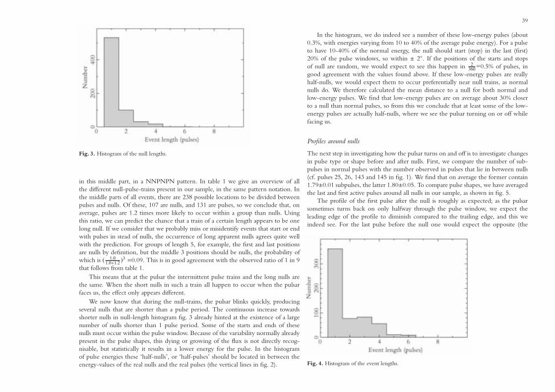
39

Fig. 3. Histogram of the null lengths.

in this middle part, in a NNPNPN pattern. In table 1 we give an overview of allthe different null-pulse-trains present in our sample, in the same pattern notation. Inthe middle parts of all events, there are 238 possible locations to be divided betweenpulses and nulls. Of these, 107 are nulls, and 131 are pulses, so we conclude that, onaverage, pulses are 1.2 times more likely to occur within a group than nulls. Usingthis ratio, we can predict the chance that a train of a certain length appears to be onelong null. If we consider that we probably miss or misidentify events that start or endwith pulses in stead of nulls, the occurrence of long apparent nulls agrees quite wellwith the prediction. For groups of length 5, for example, the first and last positionsare nulls by definition, but the middle 3 positions should be nulls, the probability ofwhich is ( 1.0

1.0+1.2 )3 =0.09. This is in good agreement with the observed ratio of 1 in 9that follows from table 1.

This means that at the pulsar the intermittent pulse trains and the long nulls arethe same. When the short nulls in such a train all happen to occur when the pulsarfaces us, the effect only appears different.

We now know that during the null-trains, the pulsar blinks quickly, producingseveral nulls that are shorter than a pulse period. The continuous increase towardsshorter nulls in null-length histogram fig. 3 already hinted at the existence of a largenumber of nulls shorter than 1 pulse period. Some of the starts and ends of thesenulls must occur within the pulse window. Because of the variability normally alreadypresent in the pulse shapes, this dying or growing of the flux is not directly recog-nisable, but statistically it results in a lower energy for the pulse. In the histogramof pulse energies these ‘half-nulls’, or ‘half-pulses’ should be located in between theenergy-values of the real nulls and the real pulses (the vertical lines in fig. 2).

In the histogram, we do indeed see a number of these low-energy pulses (about0.3%, with energies varying from 10 to 40% of the average pulse energy). For a pulseto have 10-40% of the normal energy, the null should start (stop) in the last (first)20% of the pulse windows, so within ± 2◦. If the positions of the starts and stopsof null are random, we would expect to see this happen in 2

360 =0.5% of pulses, ingood agreement with the values found above. If these low-energy pulses are reallyhalf-nulls, we would expect them to occur preferentially near null trains, as normalnulls do. We therefore calculated the mean distance to a null for both normal andlow-energy pulses. We find that low-energy pulses are on average about 30% closerto a null than normal pulses, so from this we conclude that at least some of the low-energy pulses are actually half-nulls, where we see the pulsar turning on or off whilefacing us.

Profiles around nulls

The next step in investigating how the pulsar turns on and off is to investigate changesin pulse type or shape before and after nulls. First, we compare the number of sub-pulses in normal pulses with the number observed in pulses that lie in between nulls(cf. pulses 25, 26, 143 and 145 in fig. 1). We find that on average the former contain1.79±0.01 subpulses, the latter 1.80±0.05. To compare pulse shapes, we have averagedthe last and first active pulses around all nulls in our sample, as shown in fig. 5.

The profile of the first pulse after the null is roughly as expected; as the pulsarsometimes turns back on only halfway through the pulse window, we expect theleading edge of the profile to diminish compared to the trailing edge, and this weindeed see. For the last pulse before the null one would expect the opposite (the

Fig. 4. Histogram of the event lengths.

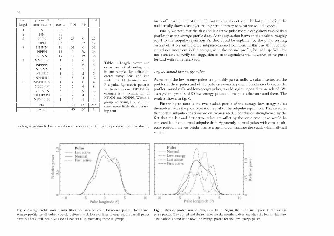
40

Event pulse–null # of totallength combinations events # N # P

1 N 3612 NN 763 NNN 27 27 0 27

NPN 52 0 52 524 NNNN 16 32 0 32

NPPN 13 0 26 26NPNN 19 19 19 38

5 NNNNN 1 3 0 3NPPPN 2 0 6 6NPPNN 1 1 2 3NPNPN 1 1 2 3NPNNN 4 8 4 12

6 NNNNNN 1 4 0 4NPPPNN 2 2 6 8NPPNPN 3 3 9 12NPNPNN 2 4 4 8NPNNNN 1 3 1 4

total: 107 131 238fraction .45 .55 1

Table 1. Length, pattern andoccurrence of all null-groupsin our sample. By definition,events always start and endwith nulls. N denotes a null,P a pulse. Symmetric patternsare treated as one: NPNN forexample is a combination ofNPNN and NNPN. Within agroup, observing a pulse is 1.2times more likely than observ-ing a null.

leading edge should become relatively more important as the pulsar sometimes already

Fig. 5. Average profile around nulls. Black line: average profile for normal pulses. Dotted line:average profile for all pulses directly before a null. Dashed line: average profile for all pulsesdirectly after a null. We have used all (500+) nulls, including those in groups.

turns off near the end of the null), but this we do not see. The last pulse before thenull actually shows a stronger trailing part, contrary to what we would expect.

Finally we note that the first and last active pulse more clearly show two-peakedprofiles than the average profile does. As the separation between the peaks is roughlyequal to the subpulse separation P2, they could be explained by the pulsar turningon and off at certain preferred subpulse-carousel positions. In this case the subpulseswould not smear out in the average, as in the normal profile, but add up. We havenot been able to verify this suggestion in an independent way however, so we put itforward with some reservation.

Profiles around low-energy pulses

As some of the low-energy pulses are probably partial nulls, we also investigated theprofiles of these pulses and of the pulses surrounding them. Similarities between theprofiles around nulls and low-energy pulses, would again suggest they are related. Weaveraged the profiles of 80 low-energy pulses and the pulses that surround them. Theresult is shown in fig. 6.

First thing to note is the two-peaked profile of the average low-energy pulsesthemselves, with the peak separation equal to the subpulse separation. This indicatesthat certain subpulse-positions are overrepresented, a conclusion strengthened by thefact that the last and first active pulses are offset by the same amount as would beexpected based on normal subpulse drift. Apparently, normal pulses with certain sub-pulse positions are less bright than average and contaminate the equally dim half-nullsample.

Fig. 6. Average profile around lows, as in fig. 5. Again, the black line represents the averagepulse profile. The dotted and dashed lines are the profiles before and after the low in this case.The dashed–dotted line shows the average profile for the low–energy pulses.

41

Fig. 7. Subpulse-pattern longitudejumps over continuous nulls. Each markis the jump over one null.a) Mapped into a region from − 3

4 P2

to 14 P2 around the expected location

in the continuous-drift case. b) Thesame data, duplicated to show subpulsegrouping, with simulated pre-nullsubpulse positions added for clarity.The vertical dashed-dotted line predictssubpulse positions for a total stop of alldrift during the null. The dashed linesare the prediction if drifting continuousduring the null as it did before, fornon-aliased drift. The dotted lines showwhich subpulses one spark makes ifthe drift is aliased. c) The same data,now with the predicted aliased subpulsepath (dotted line), and the actual lowerdriftrate.

Position jumps over nulls

Looking at the subpulse drift in PSR B0818−13 in fig. 1, the drift direction seems ob-vious (slowly towards earlier arrival) but in reality it might be different. The subpulseslack clear, recognisable traits (width, height or spacing) so instead of moving slowlytowards earlier arrival, the subpulses might actually move more quickly towards laterarrival, and still produce the same image as fig. 1. As we only observe the subpulseposition once per pulse period, we undersample the subpulse movement and cannotdetermine the underlying speeds immediately (also see fig. 2 in Chapter 2).

By focusing on drift behaviour around nulls, we hope to obtain more informationabout the subpulse-drift alias mode and the rotation speed of the underlying carousel,like we previously did for PSR B0809+74 (Chapter 2). For each null in our sample,we determine the positions of the preceding and following subpulses and calculate thephase jump of the subpulse system over each null.

In fig. 7a we plot the longitude jump of the subpulse system versus null length,for all nulls in our sample. As the subpulses are indistinguishable, it is not clear whichpre-null subpulse corresponds to which post-null subpulse. Therefore, in fig. 7a, allthe data is mapped into one region that is P2 (the average subpulse separation) wide.

To visualise the data better, we have recreated the subpulse pattern by duplicating thedata-points with offsets of N×P2 in fig. 7b. The real grouping of the subpulses is nowmuch more apparent. This diagram is analogous to fig. 1, but is now thought to showthe drifting of the subpulses during the null, when they are not actually visible. Wehave also added some simulated pre-null subpulse positions in the lower half of thediagram, for clarity.

If, during the null, the subpulse would stop drifting, the subpulses should followthe vertical dashed-dotted line in fig. 7b. If the subpulses continue to drift during thenull, they should follow the dashed line. Neither of the two is a particularly goodfit. After the null, the subpulses appear to outrun the prediction-line, which wouldindicate the drift-speed has increased during the null.

The subpulse drift alias mode

For the dashed line in fig. 7b we have assumed that the drifting is not aliased, i.e. thatone driftband is made by only one spark. Another option would be that the carouselis rotating the other way (as in fig. 2b in Chapter 2). In this case, a single spark does

42

not move towards earlier arrival and follow the dashed line in fig. 7b. It moves towardslater arrival and follows one of the dotted lines.

Compared to these dotted lines of expected positions, the post-null subpulses arelagging, which means the drifting slows down during a null. This would be consistentwith the behaviour of the only other well-studied case of drifting-nulling interaction,in PSR B0809+74. There the spark-carousel unambiguously decelerates during anull, even to the point of a total stop. If we assume that our two-pulsar sample behavessimilarly instead of oppositely, the spark carousels in both should slow down duringnulls, and therefore the real drift direction in PSR B0818−13 must be towards laterarrival. It could do so as illustrated by the dotted lines in fig. 7b, but faster too. Ifwe assume the carousel consists of 20 sparks, similar to PSR B0943+10 Deshpande &Rankin (1999) and PSR B0809+74 (Chapter 2), we can place an upper limit on thecarousel rotation time. In the slowest aliased case, it takes a subpulse 1.3 pulse periodsP to reach the position of its neighbour (i.e. the vertical spacing of the dotted linesin fig. 7b). The whole carousel then rotates in 1.3×P×Nsparks ∼30s. This alreadymakes PSR B0818−13 the pulsar with the fastest carousel rotation time known; if thesubpulse drift is more strongly aliased, the rotation time is even smaller.

Subpulse drift during intermittent nulls

If the carousel in PSR B0818−13 slows down during a null, then why doesn’t it stoplike the carousel in PSR B0809+74 does? Again, the answer is in the intermittentnature of the apparent long nulls. What appears to be a long null is actually a series ofshort nulls: during each of these the carousel may slow down, only to speed up againin between. On average, this comes down to a steady lower carousel speed duringnulls. In fig. 7, this would translate to a straight line through the post-null subpulsegroups, and this is in good agreement with the data, as the full line in fig. 7c shows.If we assume the alias mode as illustrated by the dotted line in fig. 7c, the averagedriftrate (full line) during a long apparent null is about 0.87±0.05 of the normaldriftrate (dotted line). Using the pulse/null ratio of 1.2 we found previously, thismeans that during the short nulls that compose this long apparent null, the drift mustbe less than half the normal driftspeed to produce the apparent driftspeed observed.

If this is correct, and the slow drift-rate seen in the apparent long nulls is due tothe subpulse drift starting and stopping every time a short null changes into a shortburst, we must find the same lower driftrate over the intermittent null-groups. In fig.8 we show the subpulse pattern over these intermittent nulls in the same fashion asfig. 8 did for continuous nulls. Again we note that the subpulses arrive earlier thanexpected. The similarity in figures 7 and 8 is striking; even in their drift-rate, thecontinuous and intermittent nulls behave identically.

Fig. 8. As fig. 7, but now for intermittent nulls.

4. Discussion

In a rotating-carousel model, the groups of subsequent short nulls and pulses can beexplained in two ways. In the one we have thus far focussed on, the entire carouselquickly stops and starts emitting. In this model all subbeams pause at the same time. Ina different model, only some subbeams in a carousel stop emitting while the carouselrotation continues, creating pulse-null patterns similar to those observed. When theoff-part of the carousel rotates into view, one observes a null. One pulse period later,an on-part might have moved into the pulse window to produce a normal pulse.Such a configuration would have to meet some very specific criteria, though. If thepattern is caused by on and off-parts of the carousel turning in and out of view, oneshould also observe half-on half-off pulses, with fewer subbeams. Yet we have foundthat the pulses in pulse-null groups contain exactly as many subpulses as normal pulsesdo. Only a carousel with many subbeams (roughly several hundreds) at a very highrotation speed could begin to explain this lack of observed on- to off-part transitions,but with a subpulse separation of 4◦, the inferred size of the total carousel appearsunrealistic.

43

When we compare pulsars B0809+74 and B0818−13, the similarities are striking.Both shine normally for 98-99% of the time, to be occasionally interrupted for severalseconds and then resume their normal emission. Both show similar changes in driftrateduring nulls. It seems clear we see the same mechanism at work in these two pulsars.Yet for PSR B0809+74 we know the long nulls must be real, as the subpulse driftstops during these nulls (Chapter 2), while in PSR B0818−13 we never see longnulls. There we observe periods of intermittent emission and quietude, in groupsabout as long as the nulls in PSR B0809+74.

Apparently, the mechanism that causes the emission in PSR B0809+74 to fullyturn off, only reaches a border-line state in PSR B0818−13. Why the chances fornull or pulse occurrence within such a state should be almost equal is unclear. Thelong timescales involved (even in the intermittent nulls) remains the biggest problem.In a polar-gap model (the basic physics of which are already debatable) for example,the potential gap over the magnetic pole can build up or discharge in microseconds(Ruderman & Sutherland 1975). Why the pulsar would flicker on a timescale ofseconds, for 10 seconds in total, as it does in PSR B0818−13 remains unclear; wehave not been able to explain this behaviour with any current pulsar theory. Whatone can do, is study the behaviour of different pulsars to find underlying patterns,which is what we have now done for PSR B0809+74 and PSR B0818−13.

The carousel rotation times found in PSR B0943+10 (41 seconds) andPSR B0809+74 (> 200 seconds) pose a similar time-scale problem; in a simple polar-gap theory, the rotation times are roughly several seconds (Ruderman & Sutherland1975) and the rotation times found thus-far are much larger. The upper limit of 30seconds we find for PSR B0818−13 extends the sample, back towards the previouslyexpected values. A theory like the abovementioned also predicts that the rotationtimes scale with pulse period P and magnetic field strength B as B

P2 , which im-plies that the rotation time of PSR B0818−13 should be 3 times longer than that ofPSR B0809+74, instead of the more than 10 times shorter we find. Our determina-tion of the carousel rotation time in PSR B0818−13 is therefore a step to finding thedependencies of carousel rotation times on other pulsar parameters empirically.

5. Conclusions

Both the apparently long nulls and the groups of intermittent nulls can be quantita-tively explained by trains of short nulls and pulses. The subpulse-drift behaviour overthe two is identical: during the nulls, the subpulse drift appears to speed up. Assumingthe underlying sparks slow down, as they do in PSR B0809+74, we conclude thatthe subpulse drift in PSR B0818−13 is aliased. This then leads to a carousel-rotationtime of less than 30 seconds, the fastest one found to date.

Chapter 4

UNUSUAL SUBPULSE MODULATION IN PSR B0320+39UNUSUAL SUBPULSE MODULATION IN PSR B0320+39

with Russell Edwards and Ben StappersWe report on an analysis of the drifting subpulses of PSR B0320+39 that indicates a sudden step of ~180 degrees in subpulse phase near the centre of the pulse profile. The phase step, in combination with the attenuation of the periodic subpulse modu-lation at pulse longitudes near the step, suggests that the patterns arise from the addition of two superposed components of nearly opposite drift phase and differing longitudinal dependence. We argue that since there cannot be physical overlap of spark patterns on the polar cap, the drift components must be associated with a kind of multiple imaging of a single polar cap carousel spark pattern. One possibility is that the two components correspond to refracted rays originating from opposite sides of the polar cap. A second option associates the components with emission from two altitudes in the magnetosphere.

' '''

47

1. Introduction

For a number of pulsars it is known that each pulse is composed of a number ofsubpulses, and that for each successive pulse the subpulses appear to ‘drift’ by a givenamount across the profile (Drake & Craft 1968). The rate at which subpulses driftacross the profile is not constant but rather depends on their pulse longitude. Thiscan be understood in the context of the widely adopted ‘carousel’ model of driftingsubpulses (Ruderman 1972), which postulates the existence of a ring of equally spaced‘sparks’ above the polar cap that give rise to ‘tubes’ of plasma streaming upward fromthe surface, ducted along magnetic field lines. At a certain altitude these particles emitmicrowave radiation that is beamed along tangents to the local field lines, giving rise toa beam pattern that consists of a ring of ‘subbeams’ (bright spots), reflecting the polarcap spark configuration. As the pulsar rotates the distant observer samples emissionalong a certain path in the beam pattern. Under the right viewing geometry, the sight-line makes a tangential pass along the ring of subbeams, giving rise to the receptionof a sequence of one to a few subpulses every time the star rotates. Due to the non-linear mapping between (spin) longitude and magnetic azimuth, the subpulses shouldappear more closely spaced around the point at which the sight-line makes its closestapproach to the magnetic pole. As the carousel slowly rotates about the magnetic pole,the longitude at which the emission from a given spark is seen exhibits a monotonicdrift with time, which by extension of the above argument is greater in magnitudefurther from the magnetic pole.

By stacking the intensity time series modulo the pulse period to produce a two-dimensional array in pulse number and pulse longitude, and taking Fourier trans-forms along constant-longitude columns (forming a longitude-resolved fluctuationspectrum; LRFS), Backer (1970a,b) was able to measure not only the characteristicperiodicity in pulse number (P3, the time taken for one subpulse to drift to the for-mer position of its neighbour), but also its amplitude and phase as a function of pulselongitude. Many subsequent studies employed this method but ignored the phase in-formation, however those that examined the longitude-phase relation (Backer 1970a;Wright 1981; Davies et al. 1984; Biggs et al. 1987; Ashworth 1988) found behaviourqualitatively consistent with that expected under the carousel model.

The longitude-phase relationship expected under the carousel model depends onthe number of sparks present, the misalignment angle between the spin and magneticaxes, and their orientation with respect to the line of sight. Hence studies of therelationship have the potential to provide valuable information about the pulsar, par-ticularly in comparison to the observed longitudinal dependence of the polarisationposition angle which, under the magnetic pole model of Radhakrishnan & Cooke(1969), depends on the same geometric parameters.

Motivated by these goals, we embarked on a program of analysis of several pulsarswith drifting subpulses using the Westerbork Synthesis Radio Telescope (WSRT).One of the target sources was PSR B0320+39. This pulsar was discovered indepen-dently by Damashek et al. (1978) and Izvekova et al. (1982) in surveys of the northern

sky at 400 and 102.5 MHz respectively. Further observations revealed the emissionof very regular drifting subpulses (Izvekova et al. 1982) which occur in two dis-tinct pulse longitude intervals, with a non-drifting component present in the averageprofile (Izvekoza et al. 1993; Kouwenhoven 2000). In this paper we report a mostunexpected result from our study of the longitude-phase relationship of the driftingsubpulses of PSR B0320+39.

2. Observations and analysis

We observed PSR B0320+39 on 2000 November 3 with the Westerbork SynthesisRadio Telescope (WSRT). Signals from fourteen telescopes were added (after ap-propriate delays) in each sense of linear polarisation in a 10MHz band centred at328MHz. These were processed using the Dutch Pulsar Machine (PuMa), operatingas a digital filterbank with 64 channels and 819.2µs sampling in total intensity (StokesI). For details of the system see Voute et al. (2002).

In offline analysis we de-dispersed the data and binned the resultant time se-ries into an array in pulse longitude and pulse number using the ephemeris ofArzoumanian et al. (1994). A total of 3400 pulses in 3701 longitude bins was recorded,with a region of 512 bins including the on-pulse used in further analysis. The samples

Fig. 1. First 100 pulses of 328 MHz timeseries for PSR B0320+39, binned in pulse longitudeand pulse number.

48

were normalised to produce an average profile with a zero baseline and a peak valueof unity. The first 100 pulses are shown in a greyscale form in Fig. 1.

The techniques employed in the further analysis are based on those presented indetail by Edwards & Stappers (2002). We computed the two-dimensional DiscreteFourier Transform (DFT) of the first 2048 pulses of the pulse longitude – pulse num-ber array to yield what we call the two-dimensional fluctuation spectrum (2DFS). Thisis mathematically equivalent to the harmonic resolved fluctuation spectrum (HRFS;Deshpande & Rankin 1999; Edwards & Stappers 2002)1, and the form of the powerspectrum found here for PSR B0320+39 matches that found by Kouwenhoven (2000)for the HRFS. For the purposes of clear display we also computed a spectrum usingdata from which we subtracted the average profile from each pulse, and padded withzeros in the longitude axis, in order to improve the resolution. The resolution inthe time-associated axis was unnecessarily high (2048 elements), so to improve thesignal-to-noise ratio we smoothed the power spectrum by convolution with a 7×1-bin (νt × νl) boxcar before plotting the relevant portion of the spectrum2 in Fig. 2.The spectrum is dominated by a pair of components associated with the drift mod-ulation; two are present because the spectrum derives from the Fourier transform ofreal-valued data (see Edwards & Stappers 2002). Also present with high significanceare a pair of responses corresponding to the second harmonic of the subpulse response.The features near νt = 0.02 and 0.04 cycles/period are significant, however they alsoappear in an analysis of off-pulse data, indicating that they are caused by periodicinterference.

After performing the 2D DFT, the complex spectrum was shifted in both axesby an amount which placed the primary response to the drifting subpulses at zerofrequency. We then masked other components present in the spectrum (namely thecomplex conjugate ‘mirror’ of the primary response, the pair of second harmonicsand the DC component) by multiplication of the coefficients with a transfer function:

f (νt) =

⎧⎪⎪⎪⎨⎪⎪⎪⎩0 |νt − νtc|/w < 0.52|νt − νtc|/w − 1 0.5 ≤ |νt − νtc|/w ≤ 11 |νt − νtc|/w > 1

(1)

where νt is the time-associated axis, νtc is the centre frequency of the component tomask, and w is the frequency extent of the region of zero transmission. The resultsthat follow derive from filters with w = 0.05 cycles/period, although as expected theywere found to be insensitive to w unless it becomes too small to mask adequately orso large that it masks some of the desired signal. We then computed the inverse DFTof the result.

1 Without the use of ‘twiddle factors’ (Cooley & Tukey 1965), the 2DFS will differ fromthe HRFS. However, it is easily shown that this merely amounts to the provision of slightlydifferent sampling lattices over the same continuous function, due to the assignment of integerpulse numbers (2DFS) versus integer harmonic numbers (HRFS).

2 The sampling interval used allows longitude-associated frequencies up to 1850 cy-cles/period, however all significant power is present in the portion of the spectrum shown.

Fig. 2. Main panel: Two-Dimensional Fluctuation Power Spectrum of PSR B0320+39. Thegreyscale saturates at 0.05 times the peak power, while the contours show the same spectrum atlevels 0.05 and 0.5 times the peak. Left panel: ‘collapsed’ spectrum formed by averaging rowsof the 2D spectrum. Bottom panel: power as a function of νl for νt = −0.118.

We represent the subpulse signal as the real part of the product of a pure two-dimensional sinusoid and a two-dimensional complex modulation envelope. By theconvolution theorem, this envelope is the result of the inverse transform performedabove. It describes the deviations from a pure periodicity of constant amplitude thatarise due to amplitude modulation at the pulse period, scintillation or nulling, non-uniform spacing of subpulses in pulse longitude (e.g. due to sight-line curvature) andslow variations in the drift rate. Using the iterative scheme of Edwards & Stappers(2002) we decomposed the two-dimensional envelope into the product of two mod-ulation envelopes that vary in pulse longitude and pulse number respectively. Such adecomposition is able to model the behaviour of a rotating carousel, where the ge-ometry defines the longitude-phase dependence and the carousel rotation determines

49

Fig. 3. Inferred modulation envelope (solid line and filled circles) and average pulse profile(dotted line). Also shown is the phase envelope computed by coherent addition of a set of 69rows (0.108 < νt < 0.128) of the 3400-pt LRFS over which significant power was seen (unfilledcircles), and the phase envelope computed by coherent addition of the peak row from each oftwenty-six 128-pt LRF spectra resulting from time-segmentation of the sequence (with thistransform length the majority of modulation power falls in a single row). The nominal phaseslope of 1/P2 = 60◦/◦ has been subtracted from the phase envelopes before plotting.

the time-phase dependence, and its basic assumptions – that the longitudinal spacingof the subpulses is time invariant, and that the time spacing of the subpulses is longi-tude independent – are in agreement with previous studies; see Edwards & Stappers(2002). The validity of this approach in the case of PSR B0320+39 was confirmedby computation of the 2DFS of the difference between the observed signal and thatpredicted using the real part of product of the two one-dimensional envelopes. Nosignificant power remained in the portion of the spectrum previously occupied by theprimary drifting subpulse response.

The spectral shifting performed earlier has the effect of removing a constant phaseslope in each of the envelopes. Since the slope varies over the envelope, the choiceof value to use in the shifting is somewhat arbitrary and was refined after viewingthe resultant envelopes. The periodicity with pulse number was well defined and avalue of P3 = −P1/0.118 was used. The response to the drifting component in theother axis is very broad, and in fact extends well into negative frequencies (Fig. 2).This complicates the choice of value for 1/P2 to be used in shifting the spectrum inthe longitude axis. We chose a value of P2 = P1/60 to give the resultant envelope arelatively small phase slope over most of the pulse3.

The inferred longitude-dependent envelope (Fig. 3) shows that nearly linear sub-pulse modulation occurs in two distinct longitude intervals, with a striking phaseoffset of ∼180◦ between them. In terms of the longitude-time diagram, the effect ofthe offset is to cause the drift band peaks in one component to extrapolate to troughsin the other and vice versa. To check this result we computed the (complex) LRFSand examined the amplitudes and phases in frequency bins near P3 = P1/0.118. Sincethe modulation is not a pure periodicity, the power is spread over several bins in thespectrum. Although of a much lower signal-to-noise ratio, the shape of the phaseenvelope in each bin was consistent with that inferred with our preferred technique,which makes optimal use of all modulation power. Similarly, division of the observa-tion into segments in time (which results in wider frequency bins and potentially alsoin reduced frequency drift in each segment) and examination of the phase relation inthe peak bin of each segment also gave consistent results (regardless of the segmentsize). In order to improve the signal-to-noise ratio of these other methods, we alsoused an iterative algorithm based on multiplication with the complex conjugate of atemplate envelope to determine the correct phases with which to add envelopes fromdifferent frequency bins or time segments (producing in effect coarse-grained versionsof the algorithm of Edwards & Stappers 2002). The resultant summed envelopes wereagain consistent with the result of our preferred algorithm (Fig. 3). As a final check,we folded the longitude-time data about the pulse number axis (modulo 1/0.118pulses) to produce an average profile as a function of drift phase and pulse longitude(Fig. 4). As with the LRFS methods, much of the modulation was lost due to the

3 Since this value does not lie on the natural grid of the DFT, the shift was actually performedin the time-longitude domain by multiplication with a complex exponential.

50

Fig. 4. Data folded at P3, as a function of pulse longitude and drift phase. Maxima and minimain each longitude bin are indicated with black and white crosses respectively. The data areplotted four times to guide the eye.

unstable drift motion, however some residual modulation remained and is sufficientto confirm the unusual phase behaviour.

Knowing that there is a ∼180◦ offset between the two halves of the subpulse phaseenvelope, we may explain two otherwise curious facts about PSR B0320+39. Thefirst concerns the values of P2 previously reported, which are around P1/120 (Izvekozaet al. 1993 report 3.1◦ of longitude, i.e. P2 � P1/116 at 406 MHz; Kouwenhoven2000 reports 24.5 ms, i.e. P2 � P1/123, at 328 MHz). These strongly differ fromour nominal P2 = P1/60 because they are based on measurements of actual subpulseseparations, which will nearly always be taken between subpulses on opposite sides ofthe phase shift. Since the subpulse in the trailing component leads (or lags) the positionit would take in a continuous linear phase envelope by ∼180◦ of subpulse phase, thederived spacing differs from that expected from the typical phase slope by a factorof 1/2 (and probably sometimes 3/2). The second curiosity explained by the phaseoffset is the local minimum in the subpulse HRFS response at around 60 cycles/period(Fig. 2). The complex longitude-dependent modulation envelope (once the constantphase slope is subtracted) is quite close to an odd real-valued function, which causesits Fourier transform to have local minimum in its power at DC. This is the cause ofthe local minimum around 60 cycles/period, the typical longitudinal drift frequency.

Without the phase offset the envelope would be close to a real-valued even functionand its Fourier transform would not have a strong minimum at its centre.

Furthermore, we note that the equivalence of the 2DFS and HRFS provides anexplanation for the apparent ‘secondary’ component at 0.118 cycles/period, suggestedby Kouwenhoven (2000) to be due to the ambiguity between which drift band joinsto which between the two components. In fact, the subpulse response is very broadin the longitude-associated frequency axis, and extends significantly into negativefrequencies. The symmetry of the two dimensional Fourier transform of real functionsis such that the power at any frequency pair νl, νt is equal to that at −νl,−νt (whereνl and νt are the frequencies in the longitude-associated and time-associated axesrespectively). If only the positive frequencies in νl are plotted, as is the case with theHRFS, no information is lost but individual components that span the νl = 0 axis willappear as two spatially separated components at νt values of opposite sign. When thefull spectrum is plotted as in Fig. 2 the proper interpretation becomes apparent.

3. Discussion and interpretation

Polar cap models

The phenomenon of drifting subpulses has been used repeatedly in investigationsof pulsar emission as a potentially strong clue about the geometry of the system.The fact that those pulsars that show nearly linear drifting subpulses tend to have adouble, ‘unresolved double’ or ‘single’ average pulse profile morphologies, with manyshowing a transition from resolved to unresolved double as the observing frequencyis increased, is usually seen as strong support for some form of ‘hollow-cone’ polarcap model (Radhakrishnan & Cooke 1969; Ruderman & Sutherland 1975; Backer1976; Rankin 1983, 1986; Lyne & Manchester 1988). PSR B0320+39 shares thesecharacteristics of regular drifting subpulses and a transition from a resolved double toan unresolved double average profile morphology between 102 MHz (Izvekova et al.1982)4 and 328 MHz (this work; also Damashek et al. 1978; Izvekoza et al. 1993).

The local steepening of the phase envelope of PSR B0320+39 in the transitionregion is inconsistent with the carousel model in its most basic form. For a single ringof ‘sparks’, as long as the sparks are elongated in either magnetic azimuth or openingangle (or neither, but not both), the subpulse modulation seen in a ring of constantopening angle has the same phase as that in any other ring, if measured from thesame fiducial azimuth. Therefore, the observed longitude-dependent subpulse phaseenvelope is directly tied to to the magnetic azimuth sampling of the sight-line viamultiplication by the number of sparks N (Edwards & Stappers 2002). The only wayto produce a sudden swing in magnetic azimuth (and hence subpulse phase) is to passclose to the magnetic pole. Such a configuration is inconsistent with the usual in-terpretation of unresolved double profile morphologies, and with the gradual linear

4 Due to an improved system response the profile of Kuz’min & Losovskii (1999) showsmuch stronger component separation than that of Izvekova et al. (1982); see fig. 6.

51

Fig. 5. Inferred subpulse phase envelope, including the 60◦/◦phase slope previously removed(indicated by the straight line). The data are plotted twice with an offset of 180◦ to facilateevaluation of the central feature as the transition between two offset regions of linear drift.Two-sigma error bars are included. The curved line represents the best fit to the data under thestandard carousel model, given the polarimetric constraint (see text).

polarisation position angle swing observed in this pulsar (Suleimanova & Pugachev2002). To prove this assertion we attempted to fit the observed subpulse phase swingwith the geometric formula of Edwards & Stappers (2002), using a χ2 minimisationalgorithm. From the figure provided by Suleimanova & Pugachev (2002) we conser-vatively estimate the range of polarization position angle gradients consistent with thedata as dχ/dφ = 12±3◦/◦(where χ and φ are the position angle and pulse longituderespectively). The parameters of the fit were required to be consistent with this gradi-ent via the geometric model of Radhakrishnan & Cooke (1969). The result (Fig. 5)clearly fails to describe the observed behaviour.

One way to produce a jump in subpulse phase is to adopt a nested ring polar capspark configuration (Gil & Sendyk 2000) and to assign the two halves of the profile torings of different opening angles and numbers of sparks. However, this would resultin a measurably different P3 unless the circulation rates of the two carousels weredifferent by a fortuitous ratio (i.e. the inverse of the ratio of the numbers of sparksin the rings). In addition, the transition from resolved to unresolved double profilewith increasing frequency could not be explained by standard radius-to-frequencymapping (RFM; Cordes 1978). Some other mechanism such as the finite beam-widthof the elementary emission mechanism (2γ−1), the finite band-width of emission at agiven radius (with attendant RFM in the effective range of radii visible), or refractivebroadening would be required to produce the profile evolution.

Double imaging of magnetospheric origin

Given the failure of the standard model to account for the observed subpulse driftbehaviour of PSR B0320+39, we develop in this section a pair of explanations basedon a simple and plausible extension of the model. Namely, we argue that the mostimportant features of the longitude-dependent subpulse modulation envelope – a lo-cal reduction of amplitude accompanied by a rapid swing in the phase angle – arethe result of destructive interference between two superposed drifting subpulse signalsof nearly opposite phase. The observed behaviour and this explanation of it can beunderstood by analogy with the phenomenon of orthogonal polarisation mode tran-sitions, where the pulsar signal is seen to consist of the incoherent sum of two signalswith nearly orthogonal polarisation states (e.g. Manchester et al. 1975; Stinebringet al. 1984). In both cases the total intensity of the two signals simply add in the aver-age profile, while the near anti-parallel nature of the vectors representing the complexsubpulse modulation signal (in the Argand plane) or the polarised part of the signal(in the Poincare sphere) explains the reduction in magnitude (subpulse amplitude,polarised intensity) and the swing in orientation (subpulse phase, polarisation positionangle) during a transition of dominance from one mode to the other. Other than theobvious features of the shift in phase and the attenuation in amplitude, the continu-ity of both the average profile and the absolute value of the gradient of the subpulseamplitude envelope serve as supporting evidence for this hypothesis.

Since the polar cap cannot be physically populated with overlapping spark systems,we argue that the superposed drifting components of PSR B0320+39 are associatedwith a form of ‘double imaging’ of the polar cap excitation pattern. Whereas thepolar cap may consist of a single, drifting ring of excitation points (e.g. sparks), thephysics that map this to a radiated beam pattern must do so under two different trans-formations that are received in incoherent addition by the observer. This gives rise toa subpulse pattern that is the sum of two overlapping components with differing peakpulse longitudes, and phases that differ in their contribution at a given pulse longitudeby a constant offset of ∼180◦. This also implies that the average pulse profile is the

52

Fig. 6. Average total intensity pulse profiles of PSR B0320+39 over a frequency range of102–1408 MHz. The profiles are normalised to the same peak intensity and (in the absenceof timing information) were aligned by eye to match the model proposed here. The 328 MHzprofile is from this work. The 102 MHz profile is that of Kuz’min & Losovskii (1999), andthe remaining profiles are from Gould & Lyne (1998). All profiles other than the 328 MHzone were obtained via the EPN profile database.

simple sum of two overlapping components approximately equal to the correspondingsubpulse amplitude envelopes.

In this section we discuss two potential mechanisms for such an effect. The firstassociates the images with different ray paths in a refractive magnetosphere (Petrova& Lyubarskii 2000), while the second attributes them to emission originating at twodiscrete altitudes in the magnetosphere (Rankin 1993). Before going into the detailsof each scenario, given that they both produce a beam consisting of a pair of nestedcones, we are are in a position to examine the consistency between these modelsand the observed pulse profile morphology. This is important because, in assigningthe two components of PSR B0320+39 to cones of different opening angles, weare abandoning the standard ‘single cone’ explanation favoured for most pulsars withregular drifting subpulses. We suggest instead that a cut through an outer cone (fromthe outside to the inside) produces a leading component, while a trailing componentis produced by a pass along the edge of the inner cone. At most radio frequencies thedifference in the opening angles of the cones is small and the components overlap, butradius-to-frequency mapping causes the outer cone to expand at lower frequencies,giving the components sufficient separation to be resolved at 100 MHz. Clearly oneshould also expect a third component to be present on the trailing edge of the profileas the sight-line passes across the outer cone for the second time. This is actuallyobserved at frequencies at and above 600 MHz (Gould & Lyne 1998), giving furthersupport to our assertion that more than one cone of emission is visible from this pulsar.As shown in Fig.6, the pulse profiles observed for PSR B0320+39 match this picturewell. We now turn to the specifics of the two mechanisms.

Refraction

Refractive effects have long been considered potentially important in pulsar magneto-spheres (e.g. Melrose 1979; Barnard & Arons 1986), particularly in the production ofcircular polarisation (Allen & Melrose 1982) and superposed orthogonally polarisedradiation (McKinnon 1992). Only recently, however, has the potential for refractionto explain pulse profile morphologies seen detailed study (Lyubarskii & Petrova 1998;Petrova & Lyubarskii 2000; Petrova 2000). Based on the simple argument that themagnetospheric plasma density has minima both at the magnetic pole and at theedges of the cone defined by the last open magnetic field lines, Petrova & Lyubarskii(2000) showed that rays emitted poleward of the peak of the plasma distribution couldbe refracted across the pole to exit with an angle to the pole of the opposite sign to thatwith which they were emitted. Rays emitted outward of the plasma peak are simplyrefracted to somewhat greater opening angles. This is illustrated schematically in Fig.7. Clearly, at any pulse longitude the observer may potentially receive two rays, onefrom either side of the magnetic pole.

In an axisymmetric plasma distribution, refraction occurs purely in the plane ofthe magnetic field lines. Petrova (2000) shows that the magnetosphere tends to con-centrate rays from within a given set of co-planar field lines into two components ofdifferent peak opening angle, corresponding to the different ray paths described above.

53

Fig. 7. Schematic illustration of the simulta-neous observability of rays from opposite sidesof the polar cap, via magnetospheric refrac-tion. The ’active’ field lines mark the peak ofthe plasma distribution at a given altitude. Thedotted lines indicate the approximate edge ofthe emitting flux tubes. The left hand ray orig-inates outside the peak of the plasma distri-bution, and is refracted further outward. Theright hand ray originates inward of the peakplasma density but is refracted across the poleto exit at the same angle as the other ray. Acarousel-like intensity pattern with 5 subbeamsis shown to illustrate the origin of the subpulsephase difference between the two componentsassociated with these ray paths.

These are associated with inner and outer components of the conal beam, which interms of explaining the morphology of pulsar average profiles serves the same pur-pose as the double cone of Rankin (1993). This grouping of rays occurs within agiven plane of field lines; all possible origins for visible rays must be co-planar, alongwith the line of sight and the magnetic axis. Therefore, to the extent that the plasmadistribution is axisymmetric, the geometric conveniences of the basic magnetic polemodel (Radhakrishnan & Cooke 1969) are preserved, including the polarisation be-haviour, and the mapping of azimuthal intensity modulations (e.g. from a plasma flowinitiated by a polar cap spark carousel) to observable drifting subpulses.

Moreover, if the polar cap pattern consists of a ring of an odd number of points ofexcitation, the subpulse pattern seen in the component associated with pole-crossingrays should be close to 180◦ out of phase with that in the other component. Theslight deviation from purely out of phase signals required to explain the finite lon-

gitude interval over which the phase transition occurs might be explained as a re-tardation effect or a refractive delay. Alternatively, inclusion of magnetospheric rota-tion effects or refraction under a moderately non-axissymmetric plasma distribution(Petrova & Lyubarskii 2000 model both but only in the context of polarisation wavemode coupling; see also Blaskiewicz et al. 1991) could potentially provide the kind ofsymmetry-breaking needed to produce subpulse phase offsets other than 0 or 180◦.The form of the beam pattern and the manner in which a rotating carousel polar capsystem maps to drifting subbeams under such conditions is yet to be investigated, toour knowledge.

We note that this model can also explain a related result concerning the drift-ing subpulses of PSR B0809+74. In chapter 5 we find that over the course of eachsubpulse, the polarisation state jumps in a regular manner from one polarisation stateto another, almost orthogonal state. This is similar to the behaviour seen in PSRB0320+39, in that the observed total intensity drifting subpulse pattern can be un-derstood as the sum of two components with a phase offset between them. However,in PSR B0320+39 the drift components cannot be associated with orthogonal polari-sation modes since the linearly polarised average profile at 408 MHz peaks in intensityat the centre of the profile (Gould & Lyne 1998), where maximal depolarisation oughtto take place, were the components orthogonally polarised. The single-pulse polari-metric work of Suleimanova & Pugachev (2002) confirms that the situation is similarat 103 MHz: significant power is present in two modes only in the profile wings.The model of Petrova (2001) for the origin of orthogonal polarisation modes offersa simple explanation for this disparity. Under that model the secondary polarisationmode is produced via the conversion of power from the ordinary mode in regions ofpropagation that are quasi-longitudinal to the magnetic field. If radiation in one ofthe conal components experiences significant conversion while the other does not,as could well occur since the ray trajectories involved are very different between thetwo, the situation is as seen in PSR B0809+74. If the configuration is not conduciveto conversion then both components have similar polarisation, as in PSR B0320+39.Since the conversion process also alters the orientation (i.e. position angle, ellipticity)of the modes, the longitude-dependent non-orthogonality of the polarisation modesreported in Chapter 5 might also receive an explanation via this effect.

Dual emission altitudes

A second potential explanation for how we receive the sum of two related subpulsesignals is that the two signals arise at different altitudes in the magnetosphere. Thisis the essence of the ‘double conal’ model of Rankin (1993), so-called because theproduction of radiation cones at two distinct altitudes in the magnetosphere givesrise to a beam pattern that consists of two nested cones. The radial separation of theemitting regions and the differential tangent angle between the active field lines andthe magnetic axis that arises as a result causes the polar cap plasma flux cone to produce

54

a wider radiation beam at the upper emission region, compared to the lower one. Ifthe height difference is large, up to four well-resolved conal profile components areproduced, while reduced vertical separation causes the components to overlap andproduce a ‘boxy’ profile shape. Fig. 8 illustrates this model as it might apply for PSRB0320+39 at 102 MHz, with the conal beams overlapping to a lesser degree than athigher frequencies.

Clearly this model is able to explain how we see superposed drifting patterns, butwe have not yet offered an explanation for why there should be a subpulse phase offsetbetween them. They arise from the same pattern of sparks (or plasma flux production)on the polar cap, yet we observe a phase difference of ∼180◦ near the profile centre.For the subpulse pattern to be delayed by P2/2 � 30 ms due to simple retardation(Cordes 1978) requires that the emission regions are separated by ∼9000 km, 1–2 or-ders of magnitude greater than the values typically inferred from profile morphologies(e.g. Gangadhara & Gupta 2001; Mitra & Rankin 2002; Gupta & Gangadhara 2003).Including differential aberration reduces this by no more than a factor of 2 (Cordes1978). Hence we consider this explanation unlikely. An alternative explanation worthpursuing in the future, but outside the scope of this work, is that a significant elec-tric field exists throughout the magnetosphere, causing particles to accelerate upwardmostly along magnetic field lines, but with some azimuthal E × B drift (e.g. Wright2003). The drift would cause the beam pattern radiated at a given height to be rotatedin magnetic azimuth by a certain amount, which may account for the subpulse phaseoffset seen here.

In any case, under this model the phase difference must ultimately be due to thedifferent altitudes at which the components originate. Since RFM must apply to theouter (i.e. upper) component to explain the 102 MHz pulse profile, the difference insubpulse phase between the components ought to be a strong function of frequency.Although this is the first study to examine the longitude dependence of subpulse phasein this pulsar, the fact that the longitude-dependent subpulse amplitude envelopesmeasured at 102 MHz and 408 MHz by Izvekoza et al. (1993) drop to close to zeroin the profile centre, just as at 328 MHz, suggests that at all three frequencies thesubpulses add destructively in this interval, and therefore that the phase differencebetween them is close to 180◦, regardless of frequency. The origin of the phase offsettherefore remains a mystery under this scenario.

4. Conclusions

The drifting subpulses of PSR B0320+39 occur in two distinct intervals of pulselongitude. Using a sensitive new technique we have shown that the extrapolation ofsubpulse drift from a given longitude interval is ∼180◦ out of phase with the subpulsesof the other. This was confirmed by analysis of the longitude-resolved fluctuationspectrum and by folding the data into profiles corresponding to different phases of thesubpulse drift.

Fig. 8. Schematic illustration of the simulta-neous observability of rays from two differ-ent emission heights (see also Fig. 7). Due tothe curvature of the magnetic field lines alongwhich the radiating particles stream, the rayfrom the upper region must come from a moreinward field line that that from the lower re-gion, if the two are to make the same angle tothe magnetic axis.

This suggests the presence of two components of nearly opposite drift phase, andbased on the forms of the average pulse profile and the longitudinal dependence ofthe amplitude of subpulses, we argued that the modes are superposed at all longitudes.The adding of intensity contributions from the two modes results in attenuation ofthe modulations in the longitude interval where the modes are of similar intensity,and produces a steep transition of ∼180◦ in the longitudinal subpulse phase envelopeat the point where the component intensities are equal.

Two specific models are suggested to explain this behaviour. Both produce anested pair of conal beams, one via magnetospheric refraction, the other via emis-sion at two distinct altitudes. The leading and trailing components are associated withouter and inner cones respectively. The second cut of the outer cone does not giverise to a component at 102 MHz or 328 MHz, but does produce a third, trailing com-ponent at frequencies above 600 MHz. The component separation increases rapidly

55

at frequencies below 328 MHz, in accordance with the expectations of radius to fre-quency mapping. The refractive scenario can explain the observed phase offset as asimple consequence of having an odd number of subbeams in the carousel, whilst un-der the dual-altitude emission model the phase offset is more difficult to understand.Planned observations of the time and frequency dependence of the phase offset, andthe behaviour of subpulses in the third component present at and above 600 MHz,should prove most helpful in the further evaluation of these models.

with Ramachandran, Joanna Rankin, Ben Stappers and Marco KouwenhovenPolarization-angle density displays are given for pulsars B0809+74 and B2303+30, which exhibit no evidence of the systematic polarization-angle rotation within individual subpulses previously reported for these two stars. The drifting subpulses of both pulsars exhibit strikingly linear and circular polarization which appears to reflect the characteristics of two nearly orthogonally polarized emission modes - alongwith the severe average-profile depolarization that is characteristic of their admixture at comparable overall intensities.

Chapter 5

PULSAR `DRIFTING PULSAR `DRIFTING -SUBPULSE POLARIZATION:SUBPULSE POLARIZATION:NO EVIDENCE FOR SYSTEMATICNO EVIDENCE FOR SYSTEMATIC

POLARIZATION-ANGLE ROTATIONSANGLE ROTATIONS

`

''

''

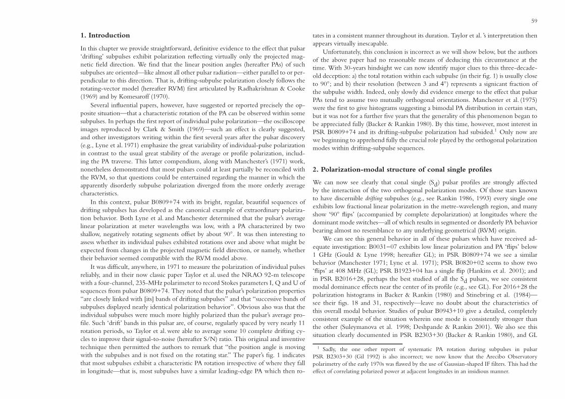
59

1. Introduction

In this chapter we provide straightforward, definitive evidence to the effect that pulsar‘drifting’ subpulses exhibit polarization reflecting virtually only the projected mag-netic field direction. We find that the linear position angles (hereafter PAs) of suchsubpulses are oriented—like almost all other pulsar radiation—either parallel to or per-pendicular to this direction. That is, drifting-subpulse polarization closely follows therotating-vector model (hereafter RVM) first articulated by Radhakrishnan & Cooke(1969) and by Komesaroff (1970).

Several influential papers, however, have suggested or reported precisely the op-posite situation—that a characteristic rotation of the PA can be observed within somesubpulses. In perhaps the first report of individual pulse polarization—the oscilloscopeimages reproduced by Clark & Smith (1969)—such an effect is clearly suggested,and other investigators writing within the first several years after the pulsar discovery(e.g., Lyne et al. 1971) emphasize the great variability of individual-pulse polarizationin contrast to the usual great stability of the average or profile polarization, includ-ing the PA traverse. This latter compendium, along with Manchester’s (1971) work,nonetheless demonstrated that most pulsars could at least partially be reconciled withthe RVM, so that questions could be entertained regarding the manner in which theapparently disorderly subpulse polarization diverged from the more orderly averagecharacteristics.

In this context, pulsar B0809+74 with its bright, regular, beautiful sequences ofdrifting subpulses has developed as the canonical example of extraordinary polariza-tion behavior. Both Lyne et al. and Manchester determined that the pulsar’s averagelinear polarization at meter wavelengths was low, with a PA characterized by twoshallow, negatively rotating segments offset by about 90◦. It was then interesting toassess whether its individual pulses exhibited rotations over and above what might beexpected from changes in the projected magnetic field direction, or namely, whethertheir behavior seemed compatible with the RVM model above.

It was difficult, anywhere, in 1971 to measure the polarization of individual pulsesreliably, and in their now classic paper Taylor et al. used the NRAO 92-m telescopewith a four-channel, 235-MHz polarimeter to record Stokes parameters I, Q and U ofsequences from pulsar B0809+74. They noted that the pulsar’s polarization properties“are closely linked with [its] bands of drifting subpulses” and that “successive bands ofsubpulses displayed nearly identical polarization behavior”. Obvious also was that theindividual subpulses were much more highly polarized than the pulsar’s average pro-file. Such ‘drift’ bands in this pulsar are, of course, regularly spaced by very nearly 11rotation periods, so Taylor et al. were able to average some 10 complete drifting cy-cles to improve their signal-to-noise (hereafter S/N) ratio. This original and inventivetechnique then permitted the authors to remark that “the position angle is movingwith the subpulses and is not fixed on the rotating star.” The paper’s fig. 1 indicatesthat most subpulses exhibit a characteristic PA rotation irrespective of where they fallin longitude—that is, most subpulses have a similar leading-edge PA which then ro-

tates in a consistent manner throughout its duration. Taylor et al. ’s interpretation thenappears virtually inescapable.

Unfortunately, this conclusion is incorrect as we will show below, but the authorsof the above paper had no reasonable means of deducing this circumstance at thetime. With 30-years hindsight we can now identify major clues to this three-decade-old deception: a) the total rotation within each subpulse (in their fig. 1) is usually closeto 90◦; and b) their resolution (between 3 and 4◦) represents a signicant fraction ofthe subpulse width. Indeed, only slowly did evidence emerge to the effect that pulsarPAs tend to assume two mutually orthogonal orientations. Manchester et al. (1975)were the first to give histograms suggesting a bimodal PA distribution in certain stars,but it was not for a further five years that the generality of this phenomenon began tobe appreciated fully (Backer & Rankin 1980). By this time, however, most interest inPSR B0809+74 and its drifting-subpulse polarization had subsided.1 Only now arewe beginning to apprehend fully the crucial role played by the orthogonal polarizationmodes within drifting-subpulse sequences.

2. Polarization-modal structure of conal single profiles

We can now see clearly that conal single (Sd) pulsar profiles are strongly affectedby the interaction of the two orthogonal polarization modes. Of those stars knownto have discernible drifting subpulses (e.g., see Rankin 1986, 1993) every single oneexhibits low fractional linear polarization in the metre-wavelength region, and manyshow ‘90◦ flips’ (accompanied by complete depolarization) at longitudes where thedominant mode switches—all of which results in segmented or disorderly PA behaviorbearing almost no resemblance to any underlying geometrical (RVM) origin.

We can see this general behavior in all of these pulsars which have received ad-equate investigation: B0031−07 exhibits low linear polarization and PA ‘flips’ below1 GHz (Gould & Lyne 1998; hereafter GL); in PSR B0809+74 we see a similarbehavior (Manchester 1971; Lyne et al. 1971); PSR B0820+02 seems to show two‘flips’ at 408 MHz (GL); PSR B1923+04 has a single flip (Hankins et al. 2001); andin PSR B2016+28, perhaps the best studied of all the Sd pulsars, we see consistentmodal dominance effects near the center of its profile (e.g., see GL). For 2016+28 thepolarization histograms in Backer & Rankin (1980) and Stinebring et al. (1984)—see their figs. 18 and 31, respectively—leave no doubt about the characteristics ofthis overall modal behavior. Studies of pulsar B0943+10 give a detailed, completelyconsistent example of the situation wherein one mode is consistently stronger thanthe other (Suleymanova et al. 1998; Deshpande & Rankin 2001). We also see thissituation clearly documented in PSR B2303+30 (Backer & Rankin 1980), and GL

1 Sadly, the one other report of systematic PA rotation during subpulses in pulsarPSR B2303+30 (Gil 1992) is also incorrect; we now know that the Arecibo Observatorypolarimetry of the early 1970s was flawed by the use of Gaussian-shaped IF filters. This had theeffect of correlating polarized power at adjacent longitudes in an insidious manner.

60

Fig. 1. Polarisation-angle-density diagram for PSR B0809+74 at328 MHz. The top panel gives the usual average Stokes parame-ters: total power I (solid line); average linear power L (=

√Q2 + U2),

corrected for the statistical bias (dashed curve); and average circularlypolarized power V (dotted curve). The usual box showing the reso-lution and off-pulse noise rms level has not been plotted because itwould be almost invisible. The central panel displays (in grey scale)the polarization position-angle distibution, where the values in eachpixel are weighted properly by the square of their S/N level (seetext). Note the two distinct ‘tracks’ corresponding to the two or-thogonal polarization modes (separated by about 90◦). A sequence oflength 3600 pulses was used. The bottom panel shows (again in grayscale) the fractional linear polarization distribution for those samplesfalling above a five standard-deviation noise threshold and weightedas in the central panel. The peak of the distribution is some 60%.

and Hankins et al. ’s work on PSRs B1540+06, B1612+07, B1923+04, B1940−12,B2110+27, and B2303+30 reveals compatible behavior. Indeed, that PSR B1923+04exhibits both behaviors (modal flips in some observations and not in others) suggeststhat modal power variations are probably common in Sd stars, where they are oftencomparable in intensity—and slight changes in their relative amplitude would producedifferent average polarization effects.

3. Observations and analysis

Our 328-MHz observation of PSR B0809+74 was conducted with the WesterborkSynthesis Radio Telescope (WSRT), using its pulsar backend, PuMa. WSRT is aneast-west array with fourteen equatorially mounted 25-m dishes. For this observation(which was made on the 26th November 2000), the delays between the dishes werecompensated, and the signals were added in phase to construct an equivalent 94-m

single dish having a sensitivity of about 1.2 K Jy−1. We also calibrated the telescopearray for polarisation measurements following the procedure given by Weiler (1973)and Weiler & Raymond (1976; 1977). With a bandwidth of 10 MHz, centred around328 MHz, the signals were Nyquist-sampled, and Fourier transformed to synthesizea filterbank of 64 complex frequency channels. Stokes parameters were computedon-line in this frequency domain. Finally, after some averaging, 2-bit (4-level) datasamples were recorded for all Stokes parameters and frequency channels, with a timeresolution of 819.2 µsec. During the offline analysis, we removed the interstellar-despersion delay between the signals of various frequency channels, producing multi-bit, floating-point sample values. For this purpose, we used a dispersion measure (DM)of 5.7513±0.0002 pc cm−3 as determined by Popov et al. (1987).

The 1380-MHz observations were also conducted with the WSRT with its pulsarbackend, PuMa. All the Stokes parameters were recorded as mentioned above, with abandwidth of 80 MHz and 512 frequency channels.

61

Fig. 2. Polarisation-angle histograms.left) PSR B0809+74 at 1365 MHz. Thetop panel gives the usual average Stokesparameters: total power I (solid line);linear power L (=

√Q2 + U2) (dashed

curve); and circularly polarized powerV (dotted curve). A box showing theresolution and off-pulse noise rms levelis just visible at the left of the dia-gram. The lower panel represents thehistogram of sample position angles withestimated errors less than 30◦ (see text),together with the superposed averagePA traverse. Note the two distict trackscorresponding to the two orthogonalpolarization modes (separated by about90◦). A 2708-pulse sequence was used.right) PSR B2303+30 at 430 MHz.Again, note the two well separatedmodal PA tracks. The display used 2370pulses and a polarization-angle thresholdof 8◦.

The 430-MHz observation of PSR B2303+30 was recorded at Arecibo on 15October 1992, using the 40-MHz correlator, which dumped the ACF/CCF’s ofthe right- and left-handed channel voltages at 1206 µsec intervals. Using 10-MHzbandwidth and retaining 32 lags, dispersion delays were reduced to negligible val-ues. The time resolution was then about 0.◦276 longitude (one rotation period equals360◦ longitude). After 3-level correction, the ACF/CCFs were calibrated and Fourier

transformed to produce Stokes parameters, which were then corrected for dispersiondelays, Faraday rotation, and feed effects (see Suleymanova et al. 1998).

Figures 1 & 2 (at 328 and 1385 MHz, respectively) represent the first availablepolarization PA histograms for pulsar B0809+74. The top and top-left panels in thesetwo figures show the usual average polarization properties: total power (Stokes pa-rameter I; solid curve), linear power, corrected for the statistical bias (dashed curve),and circular power (V ; dotted curve). The middle panel of Fig. 1 and the bottom-left

62

panel of Fig. 2 then give the PA distribution information: in the former as a grey scalewith the values contributing to each pixel carefully weighted in order to maximizetheir significance; and in the latter as a display of sample values comprising a densityplot. In the first figure, the values contributing to a pixel were weighted accordingthe square of their S/N values—after taking care to estimate the PA error accordingto the procedure given in Rankin & Rathnasree (1997; see footnote 11); whereas inthe latter the PA values are given as dots corresponding to all data samples for whichthe error in the PA, σχ (= σon/L) was less than 30◦. The on-pulse noise level σon

was estimated as σoff(Isys + L)/Isys, where Isys is the total power corresponding tothe system temperature and σoff is the standard deviation of the noise in Stokes pa-rameter I well away from the pulse window. (Clearly, σoff/Isys = (2τ∆ν)−

12 , where

∆ν is the total bandwidth and τ the effective integration time.). Finally, the bottompanel of Fig. 1 gives the density of the fractional linear polarization, also as a greyscale—where a fully black pixel represents a value of about 60%. Here, in addition toS/N weighting as above, a threshold of 5 σon was imposed to improve the quality ofthe display. This detailed analysis and display was possible for the 328-MHz sequence,because the average S/N was relatively high, but was not practical for the other twosequences.

For both pulsars in Fig. 2 the two parallel tracks—corresponding to thetwo orthogonal modes, separated by about 90◦—can be very clearly seen. ForPSR B0809+74 at the lower frequency, the two modes have comparable powerthroughout much of the pulse, resulting in severe depolarization; whereas at the higherfrequency we see little secondary-mode (herafter SPM) emission during the first halfof the pulse, so that most of the depolarization occurs after the peak of the aver-age profile. We can also see here that the PA-traverse rate associated with this SPMemission is −2◦/◦ or steeper, a fact that cannot readily be determined from the usualaverage polarimetry (e.g., the otherwise very well measured profiles recently of GL)as well as one having considerable importance for future efforts to understand theconfiguration of this pulsar’s rotating subbeam system. These PA tracks can now beassessed and interpreted according to the RVM of Radhakrishnan & Cooke (1969)—and the initial evidence here is that they are nearly, but not precisely, orthogonal.

We further note that while the PA histograms clearly exhibit the modal nature ofthe polarized power in pulsars B0809+74 and B2303+30, these distributions remainremarkably complex. The widths of the primary polarization-mode (hereafter PPM)and SPM distributions is very different. When the two modal contributions haveabout equal power, some of the radiation will be randomly polarised (as can be clearlyseen in the figures); whereas, when one dominates the other, its PA determines theensemble PA. Statistical theory discussions of this phenomenon are rather complex(see Davenport & Root 1958; Moran 1976; and especially McKinnon & Stinebring1998).

Finally, the color polarization display in Figure 3 provides a completely differentway of looking at the polarization characteristics of the subpulses. The four columns

give the total power, fractional linear polarization (corrected for statistical bias), po-larization angle, and fractional circular polarization of the first 200 pulses of the 328-MHz sequence of Fig. 1—all color-coded according to the respective color scalesat the far left of the display. Immediately, we see the drift bands—with the individ-ual subpulses drifting from left to right (the pulses are numbered from the bottomto top), the three nulls, and the fairly consistent, about 40% level of fractional lin-ear polarization. More arresting, however, are the associated polarization angle andcircular-polarization behavior, where we find two strongly preferred values for boththe PAs—nearly orthogonal values coded chartreuse and magenta, respectively, andrespective 40% negative and positive fractional circular values, coded purple and or-ange.

Careful inspection of the pulse-sequence PA behavior in the figure shows thatthere are very frequent 90◦ flips —usually from about −20◦ (magenta) to +70◦(chartreuse)—but no good example of systematic rotation. Of course, we see vari-ations which may be partly modal and partly the effect of the noise, but were thepulsar subpulses are strongest (e.g., between number 18 and 27) the modal flips areclearly seen in every pulse. We do see the longitude of these flips occuring at pro-gressively earlier phases, so as to remain approximately parallel to the drift-band andthus within the subpulses as they drift—and it was a smeared out signature of thisphenomenon which Taylor et al. recorded 30 years ago.

The full story is, however, much more complex: there is a progressive mixingof the two polarization modes as the subpulses drift across the profile window—assubpulses at the extreme edges tend to exhibit only one of the modes. In this context,the constancy of the fractional linear polarization is striking; indeed, one gets theimpression that most of individual samples are not modally depolarized—only thecontrasting (dark blue) ones which usually lie close to the PA flips. Also intriguing isthe circular, which is highly correlated with the modal linear power, while exhibitinga slightly displaced distribution along the drift bands. We will return to these questionsin much more detail in subsequent papers on PSR B0809+74.

4. Discussion

Polarisation position-angle displays for PSR B0809+74 and PSR B2303+30, com-puted from well measured sequences and given above, show clearly that the PAs traceout two well defined, nearly parallel trajectories (separated by approximately 90◦) asa function of longitude. As such, they individually trace curves which are completelycompatible (within their errors) with the Radhakrishnan & Cooke (1969) RVM,and thus entirely exclude the large (∼90◦), extraordinary, subpulse-related PA rota-tions previously reported for these two stars. If such systematic rotations occurred, thecharacter of the distributions would have to be very different—and the Taylor et al.result—about 90◦ PA rotation across subpulses occurring over a subpulse-width-orderinterval of longitude is completely explained by the the prominent, stongly longitude-segregated regions of modal power, together with their subpulse-width-order instru-

63

Fig. 3. Color display of a 200-pulse portion of the 328-MHzobservation in Fig. 1. The first column of the displays givesthe total intensity (Stokes parameter I), with the vertical axisrepresenting the pulse number and the horizontal axis pulselongitude, colour-coded according to the left-hand scale ofthe top bar to the left of the displays. The second and thirdcolumns give the corresponding fractional linear polarisation(L/I =

√Q2 + U2/I) and its angle (χ = 1

2 tan−1U/Q), ac-cording to the scales at the top-right and bottom-left of theleft-most panel. The last column gives the fractional circu-lar polarisation (V/I), according to the scale at the bottom-right of the left-hand panel. Plotted values have met a thresh-old corresponding to 2.5 standard deviations of the off-pulsenoise level. Note the strikingly modal character of the po-larized power, with the linear assuming nearly orthogonalangles—color-coded as either chartreuse or magneta—andwith the corresponding circular falling at about 40% negative(purple) and positive (orange), respectively. It is also notablethat the PAs exhibit (apart from noise variations) virtuallyonly these angle values, so that with a single pulse or sub-pulse, we see not primarily rotation, but modal 90◦ flips. Canit be any wonder that polarization behavior of such remark-able complexity caused so much early confusion?

64

mental resolution. Of course, we can say nothing about any small extraordinary PArotation within the respective PPM and SPM tracks—but this question is well beyondthe limited scope of our paper.

Nonetheless, we also see here that the character of the modal emission is exceed-ingly complex, entailing at least four factors: a) its overall angular and/or temporaldistribution—probably following from its generation within a rotating subbeam sys-tem, b) our viewing geometry, which determines the manner in which the profilewindow weights the various contributions, and c) the level of instrumental noise.The PA distributions for PSR B0809+74’s two modes at 328 MHz, for instance, arequite different; the PPM’s PA width is much broader than the SPM and their separa-tion may not be just 90◦. For all these reasons the depolarization in this pulsar is verycomplex, such that the individual pulse polarization—which is typically 40% linearand circular—is reduced in their aggregation to hardly 5 and 10%, respectively.

Consequently, it should perhaps neither be surprising that PSR B0809+74’s sub-pulses appeared to exhibit the extraordinary PA rotation on the basis of early obser-vational and analytical methods, nor that it has taken fully 30 years to discern thatthis interpretation was incorrect. Thus, we now hope and trust that this truer, moreuniversal characterization of the pulsar’s polarized emission will facilitate broader andmore comprehensive physical explanations of its overall nature.

with Aris Karastergiou, Simon Johnston, Dipanjan Mitra and Russell EdwardsWe present a study of single pulses from nine bright northern pulsars to investigate the behaviour of circular polarization, V. The observations were conducted with the Effelsberg 100-m radio telescope at 1.41 and 4.85 GHz and the Westerbork radio telescope at 352 MHz. For the first time, we present the average profile of the absolute circular polarization |V| in the single pulses. We demonstrate that the average profile of |V| is the distinguishing feature between pulse components that exhibit low V in the single pulses and components that exhibit high V of either handedness, despite both cases resulting in a low mean. We also show that the |V| average profile remains virtually constant with frequency, which is not generally the case for V, leading us to the conclusion that |V| is a key quantity in the pulsar emission problem.

Chapter 6

|V|: NEW INSIGHT INTO THE CIRCULAR|: NEW INSIGHT INTO THE CIRCULARPOLARIZATION OF RADIO PULSARSPOLARIZATION OF RADIO PULSARS

67

1. Circular polarisation in pulsars

Radio emission from pulsars is highly polarised. Occasionally the linear polarisationL is extraordinarily high, sometimes close to 100% of the total radio emission, andthe circular polarisation V is amongst the highest observed in natural sources of elec-tromagnetic radiation. Typically, however, it is only a small fraction of the total pulsaremission, although in some cases it can be much larger (i.e. ∼60% in PSR B1702−03in Radhakrishnan & Rankin 1990). The polarisation of pulsar emission has beenattributed to the emission mechanism itself and to propagation effects in the pul-sar magnetosphere (e.g. Melrose 2000). Simultaneous, multi-frequency observationsin full polarisation have shown irregularities in the polarisation of single pulses atdifferent frequencies, which have been considered direct observational evidence ofpropagation effects (Karastergiou et al. 2001, 2002; Karastergiou, Johnston & Kramer2003).

Average pulse profiles of radio pulsars are known to stabilise after the integrationof a sufficient number of pulses. This also holds for the polarisation profile, althoughthe stabilising time-scales for polarisation are longer than for total power (Rathnasree& Rankin 1995). Inspecting such average profiles, Rankin (1983a, b, 1986) claimedthat there is a difference in the circular polarisation in central or core components fromthat in outer, cone components, thought to originate in cones of emission around themagnetic axis. More specifically, core components exhibit a higher degree of V in theintegrated profile than cone components, often characterised by an “S”-shaped swingfrom one to the other handedness (Clark & Smith 1969). On the other hand, conecomponents are weakly circularly polarised in comparison to their core counterparts.In fact, it was such differences, combined with a difference in the spectral behaviourof core and cone components, that led Rankin to suggest that there is a fundamentaldifference in the emission mechanism between core and cone components.

Despite the efforts, it remains unclear whether V is intrinsic to the emission mech-anism, propagation generated, or even both. Cordes, Rankin & Backer (1978) discov-ered that in PSR B2020+28, the handedness of circular polarisation was associatedwith the polarisation position angle of the linear polarisation. In individual pulsesfrom this pulsar, where the position angle occasionally jumps abruptly by 90◦ at cer-tain pulse longitudes, these jumps where accompanied by a sense reversal in V . Theidea that V is tied to the orthogonal polarisation mode (OPM) phenomenon in pul-sars was taken further by Stinebring et al. (1984a, b) and more recently McKinnon &Stinebring (2000) and McKinnon (2002). An investigation of the same issue in PSRB1133+16 using simultaneously observed single pulses at 1.41 GHz and 4.85 GHz,demonstrated that the V - OPM association can be seen at both these frequencies, itis however stronger at the lowest of the two (Karastergiou et al. 2003).

In many cases, the longitude-resolved distributions of V in the single pulses aremuch broader than the instrumental noise, despite having a mean very close to zero.It can be easily inferred that such broad V distributions with an almost zero mean,denote a number of highly circularly polarised single pulses. Integrated profiles of

pulsars with a very low mean V , however, obscure the information that single pulsesmay be individually highly circularly polarised.

In this letter we present high quality single-pulse data from 9 pulsars, observed at3 widely spaced frequencies. We investigate the behaviour of V , by defining |V | in thesingle pulses and looking at differences between V and |V | in components that havebeen classified in the literature as of core and cone origin. We also take advantage ofthe three observed frequencies and discuss the frequency evolution of |V | as comparedto V .

2. The data

The observations

The data presented here were obtained with the 100-m radio telescope in Effelsbergand the Westerbork Synthesis Radio Telescope. They consist of single pulse sequencesfrom nine bright northern sky pulsars. The Effelsberg observations were made at 4.85GHz and 1.41 GHz between July and September 2002. Details of the receivers andthe calibration procedures of the multiplying polarimeters used can be found in vonHoensbroech & Xilouris (1997). In short, both systems have an equivalent system fluxdensity of ≈20 Jy. For the 4.85 GHz observations a bandwidth of 500 MHz was used,imposing restrictions on the resolution due to dispersion smearing. At 1.41 GHz,where dispersion smearing is significantly greater, bandwidths of 10, 20 and 40 MHzwere used depending on the dispersion measure of the pulsar.

The 352 MHz observations, 30 minutes per pulsar, were conducted with theWSRT on March 8th and 9th, 2003. The WSRT consists of fourteen 25-m dishes inan east-west array, which can be combined to form a 94-m single dish equivalent. Theequivalent flux density of the system was ≈120 Jy. We applied the schemes describedby Weiler (1973) and Edwards et al. (2003) to calibrate the data. Bandwidths of 10MHz were processed by the backend system PuMa (Voute et al. 2002), acting as adigital filter-bank. The data were 4-bit sampled at between 0.2048 and 0.8192 ms,for between 32 and 1024 channels, depending on the pulsar period and dispersionmeasure, and de-dispersed offline.

Absolute circular polarisation

We define the quantity |V | in the single pulses as the absolute value of V in everyphase bin of every individual pulse (Karastergiou et al. 2001). By taking the absolutevalue of the V data stream, we are also altering the statistics of the instrumental noise,which is no longer normally distributed and has a non-zero mean. We subtract thispositive mean from every single pulse and integrate |V | in all the pulses to produce anaverage |V | profile. Subtracting the aforementioned offset from the single pulses hasthe result of an |V | profile which can be closer to zero than the profile of V . Thishappens in cases of low |V | in the single pulses, where subtracting the offset has the

68

Fig. 1. Profiles of PSRs B0450+55,B0950+08 and B1133+16 observed atthree frequencies. The solid line repre-sents the total power, the dashed line rep-resents V and the dotted line |V |. For clar-ity, the linear polarisation is not plotted.

effect of removing part of the signal. Full details of the data analysis and the statisticsof |V | are outlined in Karastergiou et al. (2004).

3. Results

The nine pulsars that we observed display a variety of features in both their totalpower profiles and their polarimetric properties. Our single-pulse observations at

three, widely-spaced frequencies give us the opportunity to trace the properties ofV in the single pulses as a function of frequency. Figs. 1, 2 and 3 show the integratedpulse profiles of the observed pulsars, together with the profiles of V and |V |. Positiveand negative values of V denote left and right handed circular polarisation respectively.The alignment of the profiles at the three frequencies observed is only approximate.

69

Fig. 2. Same as Fig. 1 for PSRsB1237+25, B1508+55 and B1933+16.

Circular polarisation in core components

PSRs B0450+55, B1237+25, B1508+55, B1933+16 and B2111+46 (in Figs. 1, 2 and3) all have identifiable core components, demonstrating steep position angle swings(Lyne & Manchester 1988) and, in most cases, a swing in the V profile from one tothe other handedness located at the same pulse phase. This can be seen most clearly inPSRs B1933+16 and B2111+46. In both these pulsars, the swing in the V profile is

evident at all three frequencies. The profile of |V | shows a minimum which coincidesexactly with V changing handedness. This is evidence that V in the single pulsesnot only has a mean of zero, but is also tightly distributed around its mean, becausea broad distribution would include pulses of high S/N of either handedness whichwould inevitably increase |V |. This indicates that the V =0 phase remains fixed in thesingle pulses. We interpret this as direct evidence that the V swing is a constant featureof the single pulses.

70

Fig. 3. Same as Fig. 1 for PSRsB2016+28, B2020+28 and B2111+46.

We also notice that the swing in V in the core component of both these pulsarssweeps across a wider pulse phase range with frequency. Apart from the two afore-mentioned pulsars, the V and |V | signature described here can also be seen in all butthe highest frequency in PSR B1508+55.

Circular polarisation in cone components

PSRs B0950+08 and B1133+16 in Fig. 1 both consist of cone components accordingto Lyne and Manchester (1988). The fact that the V profiles at 1.41 and 4.85 GHzare very weak is in accordance with the statement that V is generally low in conecomponents (e.g. Radhakrishnan & Rankin 1990). However, as can be seen in Fig.1, |V | is quite high in these components at these frequencies, making it comparable to

71

V in the core components of other pulsars in our sample. The mechanism, therefore,that is responsible for circular polarisation in the single pulses appears to be almostequally efficient between core and cone components.

Frequency dependence of V and |V |Apart from the observation that the cone components in PSRs B0950+08 andB1133+16 show high |V |, our data permit an investigation of V and |V | as a functionof frequency. At the lowest frequency, V is negative in both pulsars and the profile of|V | is approximately a mirror image of that of V . At 1.41 GHz, V is significantly lessthan at 352 MHz. The profile of |V | however is similar to that at 352 MHz. This canbe caused by V in the single pulses being symmetrically distributed around zero, albeitwith cases of large deviation from the mean. The fraction |V |/I in the single pulses isapproximately the same between these two frequencies and it is the symmetrical dis-tribution of V around zero in the single pulses, that causes the V profile to be almostzero. Moving further up in frequency, the 4.85 GHz profile of V has a more complexstructure, with a number of phases of transition between left and right handedness.Despite this, the profile of |V | remains the same even at this frequency for both pul-sars. The constance of the |V | profile with frequency regardless of the changes in Vconstitutes evidence that |V |, the flux density of the circularly polarised componentof the radiation, is a fundamental quantity of the emission process.

PSR B2016+28 in Fig. 3 shows the |V | profile to be wider than the V profile atthe two lowest frequencies. Especially at 1.41 GHz, at either side of the V componentthe |V | component drops to zero slower. In the leading edge of the component, itappears as thought V is slightly left handed, but despite the change in handedness,the |V | profile is approximately the same fraction of I as at 352 MHz. This change ofhandedness appears to be part of a smooth change with frequency, which is responsiblefor the 4.85 GHz profile being on average slightly left handed across the pulse. Itseems, therefore, that this pulsar resembles PSRs B0950+08 and B1133+16. In fact,Figs. 1, 2 and 3 show that |V | is much less dependent on frequency than V itself. The4.85 GHz data may be slightly harder to interpret, because of a lack of S/N in thesingle pulses, but there is no pulsar that behaves contradictory to the above statementat 4.85 GHz.

The orthogonal polarisation mode phenomenon and |V |Both PSR B0950+08 and B1133+16 are pulsars that show OPM jumps in the in-tegrated polarisation profiles. The OPM phenomenon has been shown to be moreprominent at higher frequencies (Stinebring et al. 1984a, b, Karastergiou et al. 2002)and it is our opinion that the V profile changes seen in these two and other pulsarsfrom our sample, are OPM related. A full discussion on this is beyond the scope ofthis letter, it is however part of the more detailed approach to the behaviour of |V | in

Karastergiou et al. (2004). The orthogonal modes have been shown to be associatedto a particular handedness of circular polarisation (Cordes et al. 1978 Stinebring et al.1984 a, b), however it has been shown recently that this association becomes weakerat higher frequencies for PSR B1133+16 (Karastergiou et al. 2003). This results ina randomisation of the handedness of the circular polarisation which effectively re-duces the mean V , but leads to a relatively high |V |. The relevance of the OPMphenomenon can be also seen in PSR B2020+28 in Fig. 3, especially at 352 MHz.In the trailing component of the pulse, V sharply turns from positive to negative andback to being slightly positive. These sudden swings, which do not seem to affectthe wider component of the |V | profile occur together with OPM jumps in the PAswing. It therefore seems that also in this case the OPM phenomenon has the effect ofreducing the mean V while |V | remains largely unaffected. This is also a good exampleof a V swing without a |V | minimum at the cross-over point, as is the case in the corecomponents. Obviously, in PSR B2020+28, at the pulse phase of the change in thesign of the mean V , the single pulses will be somewhat circularly polarised, with casesof either handedness and a mean of zero.

4. Conclusions

We have demonstrated that accompanying the integrated profile of V with the profileof |V | provides important information on the behaviour of circular polarisation inpulsar radio emission. Making use of this simple quantity, which requires single pulseobservations, has immediately revealed new properties in a group of otherwise wellstudied bright stars. We have shown that:

1. In the pulsars that exhibit a sign change signature in the core components, a min-imum in the |V | profile is seen to coincide with the point V changes handedness.We consider this direct evidence that the phase where the mean V is 0, must haveV ≈0 also in the single pulses and, subsequently, that the swing signature is alsoconstant in the single pulses. Multiple frequency observations demonstrate thatthis fact is true at all observed frequencies.

2. In a number of cases, the profile of |V | resembles the profile of I, regardless ofthe complicated structure seen in V . This is also seen to be frequency indepen-dent. Complicated V profiles are seen in pulsars where the OPM phenomenon isobserved, and, as such, appear predominantly towards the higher frequencies.

3. In pulsars with cone components, we have shown that the very weak V profilesthat may be due to the OPM phenomenon, show comparatively high |V |. Thisdemonstrates that the single pulses may occasionally be highly circularly polarised,but average out to zero.

Points (i) and (iii) indicate that the difference in terms of V between core and conecomponents is related to how constant the V features are in the single pulses. Thisis also in accordance with the observation that core components are more stationary

72

in phase with respect to their cone counterparts that often tend to jitter. Suchjittering of a component which is partially left- and partially right-hand circularlypolarised will have the effect of reducing V , while |V | should survive. All threepoints mentioned above warrant further investigation using |V | to determine moreaccurately the nature of V in pulsars. They convincingly suggest once again, that inthe effort for progress in solving the pulsar emission mechanism problem, single pulseobservations carry vital information that should not be underestimated and lost dueto integration.

with Frank VerbuntSeveral recent papers conclude that radio-pulsar magnetic fields decay on a time-scale of 10 Myr, apparently contradicting earlier results. We have implemented the methods of these papers in our code and show that this preference for rapid field decay is caused by the assumption that the beaming fraction does not depend on the period. When we do include this dependence, we find that the observed pulsar properties are reproduced best when the modelled field does not decay. When we model the magnetic fields of new-born neutron stars by a single distribution sufficiently wide to explain magnetars, the magnetic field and period distri-butions we predict for radio pulsars are wider than observed. A bimodal distribution does explain the observed period and magnetic field distributions, independent of the use of a critical field line.

Chapter 7

MAGNETIC FIELD DECAY VERSUSMAGNETIC FIELD DECAYVERSUSPERIOD-DEPENDENT BEAMINGDEPENDENT BEAMING

75

1. Introduction

Already before the first pulsars were discovered, the theoretical prediction was madethat a neutron star with a strong magnetic field would lose rotation energy by theemission of electro-magnetic radiation, and thus that its rotation period would in-crease (Pacini 1967). The subsequently observed increase in the periods of all four firstdetected pulsars supported the idea that pulsars are neutron stars with strong (∼>1012 G)dipolar magnetic fields. Neutron stars in high-mass X-ray binaries also showed evi-dence of such high fields (e.g. Trumper et al. 1978).

Soon after, several lines of evidence appeared to indicate that the strength of themagnetic field disappears on a time scale of several million years: the lack of old, long-period pulsars and the weaker magnetic fields seen in pulsars with higher characteristicages τc ≡ P/(2P) (Gunn & Ostriker 1970); pulsars apparently stopped emitting beforethey reached a large distance from the galactic plane (Taylor & Manchester 1977); theaccreting neutron stars in low-mass X-ray binaries, which are generally old, show nosigns of strong magnetic fields. Subsequently, however, all of these lines of evidencewere shown to be misleading. The absence of long-period pulsars can be explained bythe decrease of luminosity and beaming fraction (Lyne & Manchester 1988; Rankin1993) with period. The large range of period derivatives P compared to a relativelynarrow range of periods P fully explains the anti-correlation of derived field strength B∝√

PP with characteristic age τc (Lyne et al. 1975). The apparent maximum distanceof pulsars to the galactic plane is an artifact of the distance determination from thedispersion measure caused by an electron layer with a finite scale height (Bhattacharya& Verbunt 1991). Several neutron stars with strong magnetic fields were discovered toreside in old binaries, in particular Her X−1 (Lamb 1981; Verbunt et al. 1990).

The main remaining argument was the careful population study of pulsars byNarayan & Ostriker (1990), which found that a single population of pulsars whosefield does not decay cannot explain the observed distributions of periods and period-derivatives. A re-investigation of this population synthesis by Bhattacharya et al.(1992), however, contradicted this result. Various other arguments led to a grow-ing perception that the magnetic field of neutron stars does not decay spontaneouslyduring the observed life time of radio pulsars: the pulsars with the highest characteris-tic ages move towards the plane, indicating their field is retained during the ∼>70 Myrit took the galactic gravitational field to reverse their initial velocity away from thegalactic plane, where they were born (Lorimer et al. 1997; Hartman et al. 1997). Thebirth rate of neutron stars derived from the observed number of pulsars is uncom-fortably high if they can be observed for a few million years only (Blaauw 1985); alonger life time solves this (Hartman et al. 1997). The birth rate problem is much ex-acerbated if the few pulsars with very low radio luminosity (such as PSR J0108−1431,Tauris et al. 1994) represent a numerous, hitherto undetected population. The an-gular momentum of pulsars with respect to the galactic center shows that pulsarswith high characteristic age are also old dynamically (Hansen & Phinney 1997). Thefield strengths of several accreting neutron stars have been estimated from their cy-

clotron resonance scattering features, and the results lie in a narrow range between(1-4)×1012 G for both young systems and systems as old as 108 years (Makishima et al.1999).

Thus, observations both of radio pulsars and of neutron stars in X-ray binariesappeared compatible with the idea that the magnetic field of a neutron star does notdecay spontaneously on a time scale shorter than ∼30−100 Myr, or alternatively thatits decay may be induced by mass transfer in a binary. It is therefore interesting that inthe last few years several studies challenge this idea, and suggest a return to the originalidea of rapid spontaneous field decay. A population synthesis by Gonthier et al. (2002)finds decay times of around 10 Myr, as does a pulsar velocity study by Cordes &Chernoff (1998) that is used for input in the population synthesis of Arzoumanian,Chernoff, & Cordes (2002). In this paper, we investigate whether we can reproducethese new results, and whether we can explain the differences with earlier results. InSect. 2, we describe the adaptations made to the computer code used in Hartmanet al. (1997) to address the new investigations. In Sect. 3 we apply the renewed codeto radio pulsars only, in Sect. 4 to both normal radio pulsars and high magnetic field‘magnetars’. A discussion of our results is given in Sect. 5.

2. The pulsar population synthesis code

The method of our population synthesis code for pulsars is as follows. We assume dis-tributions for the parameters of newly born pulsars, in particular their location in thegalaxy, their velocity, their pulse period and their magnetic field strength (or equiva-lently, period derivative). We then choose an age of the pulsar between zero and theHubble time and evolve the pulsar properties. The pulsar position and velocity changeunder the influence of the gravitational field of the galaxy. The pulsar period and pe-riod derivative change according to PP = 1039B(t)2, where B is the magnetic field,which we assume to decay exponentially on a time scale τ: B(t) = B(0) exp−t/τ. Fromthe new period we derive a beaming fraction, and compare it with a random numberto decide whether the pulsar is retained. If so, we compute the radio luminosity fromthe period and period derivative. If the pulsar is above the death line in the period vs.period derivative diagram, the flux is computed from luminosity and position in thegalaxy, and it is then checked whether any of four large surveys would have detectedthe pulsar. This procedure is repeated until we have simulated 2000 detections, andthe properties of this simulated population are compared with those of the real pulsarpopulation. An important feature is that we also test the real pulsars against out surveyssimulations. Only the detected set is used for comparison. This reduces the impact ofthe simplification one necessarily makes in describing the surveys.

Our assumptions for the initial distributions and for the laws of their evolution canbe varied to search for an optimum solution. To determine the optimum we comparespecifically the observed and simulated distributions of the pulse period, the magneticfield strength, the projected dispersion measure DMsin b and the radio luminosity

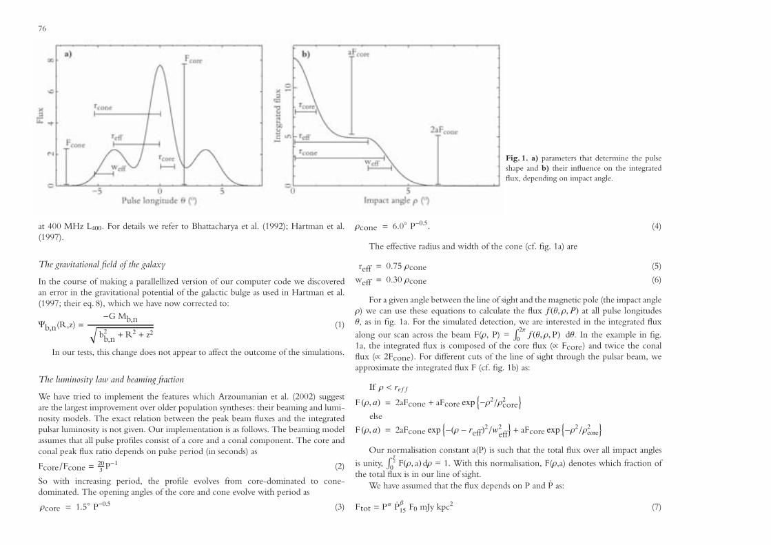
76

Fig. 1. a) parameters that determine the pulseshape and b) their influence on the integratedflux, depending on impact angle.

at 400 MHz L400. For details we refer to Bhattacharya et al. (1992); Hartman et al.(1997).

The gravitational field of the galaxy

In the course of making a parallellized version of our computer code we discoveredan error in the gravitational potential of the galactic bulge as used in Hartman et al.(1997; their eq. 8), which we have now corrected to:

Ψb,n(R,z) =−G Mb,n√

b2b,n +R2 + z2

(1)

In our tests, this change does not appear to affect the outcome of the simulations.

The luminosity law and beaming fraction

We have tried to implement the features which Arzoumanian et al. (2002) suggestare the largest improvement over older population syntheses: their beaming and lumi-nosity models. The exact relation between the peak beam fluxes and the integratedpulsar luminosity is not given. Our implementation is as follows. The beaming modelassumes that all pulse profiles consist of a core and a conal component. The core andconal peak flux ratio depends on pulse period (in seconds) as

Fcore/Fcone = 203 P−1 (2)

So with increasing period, the profile evolves from core-dominated to cone-dominated. The opening angles of the core and cone evolve with period as

ρcore = 1.5◦ P−0.5 (3)

ρcone = 6.0◦ P−0.5. (4)

The effective radius and width of the cone (cf. fig. 1a) are

reff = 0.75 ρcone (5)

weff = 0.30 ρcone (6)

For a given angle between the line of sight and the magnetic pole (the impact angleρ) we can use these equations to calculate the flux f (θ, ρ, P) at all pulse longitudesθ, as in fig. 1a. For the simulated detection, we are interested in the integrated flux

along our scan across the beam F(ρ, P) =∫ 2π

0f (θ, ρ,P) dθ. In the example in fig.

1a, the integrated flux is composed of the core flux (∝ Fcore) and twice the conalflux (∝ 2Fcone). For different cuts of the line of sight through the pulsar beam, weapproximate the integrated flux F (cf. fig. 1b) as:

If ρ < re f f

F (ρ, a) = 2aFcone + aFcore exp{−ρ2/ρ2

core}

else

F (ρ, a) = 2aFcone exp{−(ρ − reff)

2/w2eff

}+ aFcore exp

{−ρ2/ρ2

core

}

Our normalisation constant a(P) is such that the total flux over all impact angles

is unity,∫ π

2

0F(ρ, a) dρ = 1. With this normalisation, F(ρ,a) denotes which fraction of

the total flux is in our line of sight.We have assumed that the flux depends on P and P as:

Ftot = Pα Pβ15 F0 mJy kpc2 (7)

77

We take α=−1.3 and β=0.4, in accordance with Arzoumanian et al. (2002). We trieda range of values for F0 from 10−3 to 103 and determined that a value of F0=2produces the best results for our simulated period, magnetic field, dispersion measureand luminosity distributions.

Arzoumanian et al. (2002) then state they apply the effects of interstellar dispersionand scattering, without giving further information. From their fig. 2 we deduce thatthe ‘standard candle’ luminosity L is smeared by a wide Gaussian distribution σlog L= 0.7. We apply the same smearing to the fluxes from eq. 7.

For each simulated pulsar, we draw random angles between the rotational axisand the magnetic pole, and between the rotational axis and observer’s direction to thedetermine the impact angle ρ. We calculate which fraction of the flux is emitted inour line of sight. From the pulsar P and P, we determine the total flux. We combinethe two with the distance to get the flux at the telescope.

Quantum critical field strength

Regimbau & de Freitas Pacheco (2001) evaluated whether wide neutron-star initialmagnetic fields distributions could explain both the properties of radio pulsars and‘magnetars’. To test whether we can reproduce these results, we have incorporatedthe quantum critical field strength of 9.5×1013G that could stop neutron stars withhigher fields from shining in radio (Baring & Harding 2001).

3. Effects of beaming models in pulsar studies.

Core-conal beam models

We have used our code, with the implementation of the beaming model ofArzoumanian et al. (2002), to search for the fits to the observed pulsar populationfor a range of decay times. We will refer to this core-cone model as model CC.Magnetic field decay times of 10 and 100 Myr produce fits of similar quality, bothacceptable (see fig. 2). As in Hartman et al. (1997), we use a Kolmogorov-Smirnovtest to determine the probability that the modelled and real distributions are the same,and use the product Qks of the probabilities for the periods, magnetic field strengths,projected dispersion measure (DMsin b) and luminosity as a figure of merit for theoverall solution.

We note that the figure of merit for the best models CC for decay times 10 and100 Myr are about a factor 10 times less likely then the best model, model A for100 Myr, from Hartman et al. (1997). Similarly, the distribution of characteristic agesτc for models CC is acceptable, but is by itself about a factor of 10 less likely thatin the best model A for 100Myr. All models A that had decay times of 10Myr werefound by Hartman et al. (1997) to be rather less likely.

As their period evolution is slowest at long periods, one expects many pulsars tohave long periods, more than observed (Lyne et al. 1985). This shortage can be ex-

plained by any mechanism that makes it harder to detect pulsars at long periods. Lyne& Manchester (1988), Rankin (1993) and Kramer et al. (1998) all find that pulsarswith longer periods have significantly narrower beams. The volume from which theyare visible (the beaming fraction) is therefore smaller, making it less likely for themto be detected. In models A with long decay times, this period-dependent beamingexplains the relative dearth of long period pulsars; models A which combine mag-netic field decay and a period-dependent beaming fraction find too few long periodpulsars.

The reason that models CC do not favour long decay times, is that their beamingfraction dependence on period is less than in models A. Models A use isotropic beamsthat scale as P−0.5. Although the opening angles of the narrow core and wide conalbeam also diminish with period as P−0.5, their combined behaviour is different in thismodel. At short periods, the beam will be core dominated and narrow. Yet towardslonger periods, the wider conal components become more prominent: at periodslonger then 0.6 seconds, all profiles will have conal components stronger than 10% ofthe peak flux, substantially increasing the volume from which they can be detected. Infig. 3b we plot the impact of this transition from core-dominated to cone-dominatedon the pulse width (and hence the beaming fraction). In fig. 3a we plot the observeddistribution of pulse width versus period, as determined by Gould & Lyne (1998) at600 and 1400MHz. These authors note the widths of the observed profiles do notchange in this range, so we assume them be applicable to the pulse widths at 400MHzas simulated by Arzoumanian et al. (2002) in fig. 3b.

Apparently, the strong preference for a short torque decay time found by Cordes &Chernoff (1998) is no longer present in their recent work (Arzoumanian, Chernoff, &Cordes 2002). This could be because Cordes & Chernoff (1998) did not take selection

Fig. 3. Pulse width versus period for a) observed sample (Gould & Lyne 1998) b) the simulateddetected pulsars using the beaming model of Arzoumanian et al. (2002).

78

Fig. 2. Comparison of period and mag-netic field distributions of real and simulatedpulsars for model CC with decay times of10Myr (top row) and 100Myr (bottom row)

effects into account, or because of the uncertainties in the proper motion, velocity andscale-height distributions they used to determine the decay time.

Apart from the different beaming models, models CC and A differ also in theirdescription of pulsar luminosities. Model A follows the Narayan & Ostriker (1990)luminosity function in computing the luminosity as the product of a model luminosity,which is a function of P and P, and a random number chosen from a distributiondescribing the spread. Arzoumanian et al. (2002) argue that all pulsars with the sameP and P have the same intrinsic (angle-averaged) luminosity and that the observedluminosity depends on the observation angle and interstellar scintillation. This wehave used in model CC (see eq. 7). As the width of the resulting observed luminositydistribution is of the same magnitude as the intrinsic spread from Narayan & Ostriker(1990), the two descriptions are computationally very similar. We therefore think thatthe different results of models CC and A are not due to the different descriptions ofthe luminosity, but to the different beaming models.

Period-independent beaming

Gonthier et al. (2002) simulate the detection of galactic populations of radio andgamma-ray pulsars and conclude that magnetic fields decay in 5 Myr. They assumethat the beaming fraction of all radio pulsars is identical. If we follow them and elim-

inate the period dependence of the beaming fraction from model A (Hartman et al.1997) we find that this variant of model A also favours short decay times (see fig. 4).In this case, magnetic field decay is needed to make pulsars turn off towards longerperiods. Yet if we do allow for a beaming fraction that decreases with period as P−0.5,as is commonly accepted (Vivekanand & Narayan 1981; Lyne & Manchester 1988;Rankin 1993), models without magnetic field decay are favoured (see fig. 5).

4. Effect of initial magnetic field distributions in studies of pulsarsand magnetars

In their model for the formation of neutron stars, Duncan & Thompson (1992) pro-pose that in some neutron stars, those born spinning faster than P∼3 ms, dynamoprocesses are efficient enough to amplify the magnetic field. These high-field pul-sars (B>1014G) they call ‘magnetars’. They are observed mostly as soft gamma-rayrepeaters and anomalous x-ray pulsars. In the neutron-star initial magnetic field func-tion this dichotomy leads to two distinct components, one for radio pulsars and onefor magnetars.

To investigate what the influence of such a bimodal distribution would be on theradio pulsar populations, we have tested scenarios in which half of the pulsars are born

79

Fig. 4. Comparison of period and magneticfield distributions of real and simulated pul-sars for a model with period-independentbeaming, with decay times of 10Myr (toprow) and 100Myr (bottom row)

with a magnetic field of 1012.3±0.3G (the best fit from model A), while the magneticfield for the other half is 1014.0±0.8G.

The absence of radio pulsars with fields over roughly 1013−1014G seems to sup-port models in which neutron stars with field strengths higher than the quantum crit-ical field strength of 9.5×1013G do not emit in radio (Baring & Harding 2001). Yetfig. 6a shows how a model without such a quantum critical field limit still producesalmost only normal-field pulsars and actually predicts very acceptable distributionsof our test quantities. The explanation lies in the rapid evolution of these high-fieldpulsars to long periods, where their luminosity and beaming fraction are low. Due tothis rapid evolution, only very few high-field pulsars are visible at any given time, butsome are. Indeed, only recently PSR J1847-0130, a pulsar with a very high inferredmagnetic field of 9.4×1013G was discovered, challenging all but the highest quantumcritical field predictions.

Regimbau & de Freitas Pacheco (2001) evaluate a similar model, using a contin-uous field input distribution of 1013.5±0.9G, no quantum critical field strength cutoffand no deathline. They find that, using such a wide input distribution, the simulationsfit the observed period and magnetic field distributions quite well. Yet when we usethe input distribution they propose, the outcome does not fit the observed samplewell (see fig. 6b). In particular, this model predicts a much wider distribution of mag-netic fields than is observed. The reason for this is that the shorter lifetime of pulsars

with Bi=1013G (compared to those with Bi=1012G) is compensated by their largerinitial numbers. As a result, the simulated distribution contains too many long-periodand high-B pulsars.

5. Discussion

As described in the Introduction, a variety of studies of radio pulsars and neutron starsin X-ray binaries indicates that the magnetic field of a neutron star does not decayspontaneously on a time scale of less than ∼100 Myr. In this paper we have investigatedwhy several recent population studies of radio pulsars suggest a shorter time scale forspontaneous field decay.

Our main result is that the models allow a trade-off between the period depen-dence of beaming of the radio emission on one hand, and the decay of the magneticfield on the other hand. The reason behind this is as follows. In a diagram where thesame magnetic field B2 ∝ PP is plotted as a function of pulse period P, the numberof pulsars does not increase with period as follows from the equation for B whichindicates a lower P, hence longer life time at large P. The observed number of pulsarsat long periods can be suppressed either by field decay, which moves pulsars to lowerB before they reach long periods, or by a reduction of the detection probability atlonger periods, e.g. by more narrow beams at longer periods. Thus we can explain

80

Fig. 5. Comparison of period and magneticfield distributions of real and simulated pul-sars for model A with decay times of 10Myr(top row) and 100Myr (bottom row)

the difference between the strong preference for rapid field decay in the studies byCordes & Chernoff (1998) and Gonthier et al. (2002), who do not include a pe-riod dependence of beaming, and the absence of such a preference in the study byHartman et al. (1997) and Arzoumanian et al. (2002), who do.

It appears to us that beaming as a function of the period is the preferred solution,both because observations of radio pulsars indicate such a dependence (e.g. Lyne &Manchester 1988; Kramer et al. 1998), and because a long time scale for field decay isin better agreement with studies of X-ray sources. However, we do think that a moredetailed study into the period dependence of beaming of radio emission, through thestudy of pulse profiles of individual pulsars, is required before definite conclusions canbe drawn. Such a study can also address the question whether the axis of the magneticfield aligns closer with the rotation axis as a pulsar evolves towards longer periods, andprovide an important handle for the discrimination between field decay and torquedecay, in the equation B2 ∝ PP sinα, with α the angle between rotation and dipoleaxis. It is worth noting that the distribution of characteristic ages τc ≡P/(2P) is re-produced acceptably only in the models with period dependent beaming and longdecay time, even though this distribution – which essentially provides the correlationbetween P and B – does not enter our figure of merit (see fig. 5). We consider thisanother argument in favour of a long time scale for field decay.

A reduced detection probability for radio pulsars at longer periods may also bethe consequence of a reduced luminosity. Such an effect is partially included in ourpopulation synthesis studies, through the dependence of the luminosity on period.However, we find that the best figure of merit of the models is determined mainlyby the distributions of the periods P and the magnetic field strengths B, and muchless so by the distributions of the projected dispersion measures DMsin b and lumi-nosities L. The reason for this is that the distribution of DMsin b also depends on thevelocity distribution of the pulsars at birth, whereas the distribution of L shows a verywide range at the same P,P combination, due to either an intrinsic spread (as in oursimulations) and/or to a wide range of interstellar scintillation (as in the simulationsby Arzoumanian et al. 2002). With suitable changes in the assumed velocity distribu-tion and in the luminosity law, one can therefore adapt the population synthesis toproduce acceptable fits to the distributions of DMsin b and of L. A more accuratelyobserved distribution of current pulsar velocities, as is coming into existence thanksto improved measurements (e.g. Brisken et al. 2002), will provide a better constraintof the population synthesis.

Contrary to what one might expect, we do not find a strong dependence of thebirth rate on the time scale of field decay. A more important factor in the birth ratecould be the number of pulsars at very low luminosity. That such pulsars exist is indi-cated both by single nearby pulsars as PSR J0108−1431 (Tauris et al. 1994) and by the

81

Fig. 6. The magnetic field distribution of real and simulated radio pulsars, using a bimodal(top) or a wider single (bottom) initial magnetic field distribution.

detections in very long observations of central pulsars in supernova remnants (Camilo2003). That they do not represent very large numbers is indicated by the failure ofdeeper surveys to detect many more nearby, faint pulsars like PSR J0108−1431. Thisis important because the birth rates that we find in the models are compatible with theobserved rates (see e.g. the discussion in Hartman et al. 1997); much higher predictedbirth rates would be unacceptable.

The population synthesis computations assume, through the relation B2 ∝ PP, thatthe period derivative P can be derived from the dipole model. Recently this assump-tion has been questioned on the basis of the observation of young (<105 yr) pulsarswith appreciable discrepancies between real age and characteristic age (e.g. Kaspi &Helfand 2002). We note that the discrepancy for young pulsars is easily explained ifthe period Po of the pulsar at birth is too close to the current period P to warrant theimplicit assumption Po

2 P2. Hence it is not obvious that the discrepancy is impor-tant for the much longer time scales (>Myr) in population synthesis. However, if thediscrepancy indicates a strong deviation of a dipole equation for P – as indicated by

the measured values less than 3 for the braking index n ≡ 2-PP/(P)2 – which persistsat higher ages, this would invalidate any population synthesis.

Finally, the observed distribution of the magnetic fields of radio pulsars peaksnear B�1012 G (see fig. 6), i.e. well below the critical field strength. We have shownthat this implies that the magnetars, neutron stars with magnetic field in excess ofthe critical field, can not be formed from a single, broad Gaussian distribution ofthe magnetic field strengths of neutron stars at birth. This contradicts the result byRegimbau & de Freitas Pacheco (2001); we have not been able to find an explanationfor this. In this respect, it is worth noting that our population synthesis is the onlyone in which the detection routines are tested directly with the observed pulsars,i.e. it is verified that our simulation would detect the actually observed pulsars. Ifwe assume a bimodal distribution of the initial magnetic field strengths as suggestedby theory (Duncan & Thompson 1992), we find that the models can explain theobserved period and magnetic field distributions. This is independent of the use ofa critical-field line or of a photon-splitting line as a limit to the detectability, i.e. thepopulation synthesis of radio pulsars at the moment does not constrain the presenceor absence of such limiting lines in the B−P diagram.

with Ben StappersWe investigate the number and type of pulsars that will be discovered with the low-frequency radio telescope Lofar. We consider di fferent search strategies for the Galaxy, globular clusters and other galaxies. An all-sky Galactic survey can be optimally carried out by incoherently combining a large number of Lofar stations (large groups of dipoles coherently combined to form a number of beams) at an observing frequency of 140MHz. In a 60-day all-sky Galactic survey, Lofar will find approximately 1500 new pulsars, probing the local population of pulsars to a very deep luminosity limit. For targets of smaller angular size, like globular clusters and galaxies, the Lofar stations can be combined coherently, increasing the sensitivity even further. Searches of nearby globular clusters can find large numbers of low luminosity millisecond pulsars (eg. over 10 new millisecond pulsars in a 10-hour observation of M15). If the pulsar population in nearby galaxies is similar to that of the Milky Way, a 10-hour observation can find the 10 brightest pulsars in M33, or pulsars in other galaxies out to a distance of 1.2Mpc. Giant pulses from Crab-like extragalactic pulsars can be detected out to several Mpcs.

Chapter 8

FINDING PULSARS WITH LOFARFINDING PULSARS WITH LOFAR

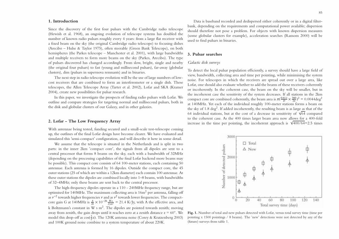
85

1. Introduction

Since the discovery of the first four pulsars with the Cambridge radio telescope(Hewish et al. 1968), an ongoing evolution of telescope systems has doubled thenumber of known radio pulsars roughly every 4 years: from a large flat receiver witha fixed beam on the sky (the original Cambridge radio telescope) to focusing dishes(Arecibo – Hulse & Taylor 1975), often steerable (Green Bank Telescope), on bothhemispheres (the Parkes telescope – Manchester et al. 2001), with large bandwidthsand multiple receivers to form more beams on the sky (Parkes, Arecibo). The typeof pulsars discovered has changed accordingly. From slow, bright, single and nearby(the original four pulsars) to fast (young and millisecond pulsars), far-away (globularclusters), dim (pulsars in supernova remnants) and in binaries.

The next step in radio telescope evolution will be the use of large numbers of low-cost receivers that are combined to form an interferometer or a single dish. Thesetelescopes, the Allen Telescope Array (Tarter et al. 2002), Lofar and SKA (Kramer2004), create new possibilities for pulsar research.

In this paper, we investigate the prospects of finding radio pulsars with Lofar. Weoutline and compare strategies for targeting normal and millisecond pulsars, both inthe disk and globular clusters of our Galaxy, and in other galaxies.

2. Lofar - The Low Frequency Array

With antennae being tested, funding secured and a small-scale test-telescope comingup, the outlines of the final Lofar design have become clearer. We have evaluated andsimulated this ’semi-compact’ configuration, and will describe it here in some detail.

We assume that the telescope is situated in the Netherlands and is split in twoparts: in the inner 2km ’compact core’, the signals from all dipoles are sent to acentral processor that forms 8 beams on the sky, each with a bandwidth of 32MHz(depending on the processing capabilities of the final Lofar backend more beams maybe possible). This compact core consists of 64 100-meter stations, each containing 50antennae. Each antenna is formed by 16 dipoles. Outside the compact core, the 45outer stations (25 of which are within a 12km diameter) each contain 100 antennae. Atthese outer stations the dipoles are combined locally into 1–8 beams, with bandwidthsof 32–4MHz; only these beams are sent back to the central processor.

The high-frequency dipoles operate in a 110 - 240MHz frequency range, but areoptimised for 140MHz. The maximum collecting area is 16m2 per antenna, falling offas ν−2 towards higher frequencies ν and as ν2 towards lower frequencies. The compact-core gain G at 140MHz is A

2k × 10−26 W sJym2 = 21.4 K/Jy, with A the effective area, and

k Boltzmann’s constant in W s m2. The dipoles are pointed towards zenith; movingaway from zenith, the gain drops until it reaches zero at a zenith distance z = 60◦. Wemodel this drop-off as cos( 3

2 z). The 120K antenna noise (Corey & Kratzenberg 2003)and 100K ground noise combine to a system temperature of about 220K.

Data is baseband recorded and dedispersed either coherently or in a digital filter-bank, depending on the requirements and computational power available; dispersionshould therefore not pose a problem. For objects with known dispersion measures(some globular clusters for example), acceleration searches (Ransom 2000) will beused to find pulsars in binaries.

3. Pulsar searches

Galactic disk surveys

To detect the local pulsar population efficiently, a survey should have a large field ofview, bandwidth, collecting area and time per pointing, while minimising the systemnoise. For telescopes in which the receivers are spread out over a large area, likeLofar, one should also evaluate whether to add the beams of these receivers coherentlyor incoherently. In the coherent case, the beam on the sky will be smaller, but inthe incoherent case the sensitivity of the system decreases. If all stations in the 2kmcompact core are combined coherently, the beam area is π( 0.61λ

D × 3602π )2 = 0.0044deg2

at 140MHz. Yet each of the individual roughly 100-meter stations forms a beam onthe sky of 1.8 deg2. If added incoherently, the resulting beam is as large as that of the64 individual stations, but at the cost of a decrease in sensitivity of

√64 compared

to the coherent case. As the 400 times larger beam area now allows for a 400-foldincrease in the time per pointing, the incoherent approach is

√400/64=2.5 times

Fig. 1. Number of total and new pulsars detected with Lofar, versus total survey time (time perpointing x 1500 pointings / 8 beams). The ’new’ detections were not detected by any of the(future) surveys from table 1.

86

Fig. 2. Number of total and new pulsars detected with Lofar in a 60-day survey, versus fre-quency observed at. The antenna optimisation for frequencies of 140MHz is the dominantfactor. To higher (lower) frequencies, the effective collecting area decreases as ν−2 (ν2).

more sensitive than the coherent approach, for the same total amount of time (alsosee Backer 1999).

In the incoherent case, one can also add the signal of the outer stations to increasethe sensitivity, without loss of field of view. While the stations in the compact coreproduce 8 beams each 32MHz wide, the 45 outer stations are limited to 32MHzbandwidth in total. To ensure uniform final beam-patterns, we split the 45 stations in8 group of 5 stations. We divide these eight groups over the eight compact core beams,each group producing a different 32MHz beam. This again increases the sensitivity by

a factor of(

64×50+5×10064×50

) (6469

) 12 = 11%. It is unclear if this increase justifies the added

complexity; the antennae could also be used for radio interference mitigation.Choosing the optimum observing frequency presents a new trade-off. To higher

frequencies, the beam size decreases as ν−2. The Lofar effective collecting area fallsoff as ν−2 above 140MHz and as ν2 below. At these low frequencies the spectralindex of the pulsar luminosity function is −1.5 (Malofeev et al. 2000), so towardshigher frequencies the pulsar brightness decreases as ν−1.5, but the sky backgrounddecreases even faster as ν−2.6 (Lawson et al. 1987). At the low frequencies, the dis-persion smearing of the pulses increases. This dispersion smearing has forced recentsurveys to observe at higher frequencies, around 1400MHz. As we coherently dedis-perse the signal, we can remove the dispersion smearing even at frequencies as lowas 140MHz. A different, but in this case more important, effect is scatter broadening:the signal passes through the interstellar medium using different paths, resulting in asignificant broadening of the pulse profile. Currently this scatter broadening cannot

be removed. The degree of scattering increases sharply towards lower frequencies, asν−4.5 (Ramachandran et al. 1997; Shitov 1994). At 140MHz, this scatter broadeningtscatt depends on the dispersion measure DM as (Shitov 1994):

tscatt = 5.2×10−7 DM3.8 ms (1)

When pulses are smeared out, the number of harmonics in the Fourier transform ofthe pulse signal decreases, causing the detection probability to drop. Although thesky background and scatter broadening increase towards lower frequency, the totalsensitivity is mainly determined by the effective collecting area: 140MHz is the mostefficient frequency to observe at (cf. fig. 2).

The minimum detectable flux Smin depends on the signal-to-noise ra-tio at which one accepts a signal as real (SNR), the system temperature(Tsys=Tantenna+Tground+Tsky), the zenith-distance dependent gain (Gz), the numberof polarisations (Npol), the bandwidth (dν), the integration time (t), the number ofincoherently added beams (N) and the pulse width (W) and period (P). As it dependson zenith distance and sky noise, Smin varies per pointing, but a typical value for Lofarusing a 60 minute integration time is

Smin = SNR(Tsys

Gα

) (N

Npol dν t

) 12 ( W

P −W

) 12

= 10

(1000K24K/Jy

) ( 69

2 32 × 106Hz 3600s

) 12(0.05s0.45s

) 12

= 2.4 mJy (2)

To determine the number and type of pulsars Lofar can find, we have used theabove characteristics to model the detection of a large number of simulated pulsars.For this, we have used a population synthesis code that simulates the birth, evolu-tion, death and possible detection of radio pulsars, as described more extensively in

Survey Year N ν (MHz)Jodrell 1972 51 408UMass-Arecibo 1974 50 430MolongloII 1978 224 408UMass-NRAO 1978 50 400Parkes Multibeam 1997-2000 1050 1374GBT 340LOFAR 140

Table 1. Name, year, number of detected pulsars (N) and frequency observed at (ν) of the sevensurveys simulated. The time per pointing for the GBT is chosen such that the total survey timeis equal to that of a Lofar survey with 1-hour pointings. Data from Davies et al. (1977); Hulse& Taylor (1975); Manchester et al. (1978); Damashek et al. (1978); Manchester et al. (2001);Hobbs & Manchester (2004).

87

Fig. 3. Pulsars discovered with theParkes Multibeam and Lofar surveys, for1-hour Lofar pointings. Left) projectedon the Galactic plane. Right) projectedon the plane through the Galactic centreand sun, perpendicular to the disk.

Hartman et al. (1997). We choose initial positions and velocities and calculate theorbits through the Galaxy (van Leeuwen & Verbunt 2004). We evolve magnetic fieldsand periods, determine whether the pulsar is still above the death-line and estimatethe luminosity at 400MHz, which we scale to the observing frequency as ν−1.5. Wedetermine the sky background for the simulated position on the sky using the skymap of Haslam et al. (1982) and the abovementioned power law with spectral index−2.6. We use the Taylor & Cordes (1993) model to estimate the dispersion measureand, using eq. 1, the scatter broadening. We then determine which of these pulsarsis detected by any of the 7 simulated pulsar surveys specified in table 1. These aremodelled using their sky coverage and sensitivity function. By comparing the sim-ulated pulsar sample with the real one, Hartman et al. (1997) have determined themost probable model parameters using the first four surveys mentioned. We use thisbest model with one modification: the number of pulsars born per unit area drops offexponentially with galactocentric radius, so the initial radius distribution is:

p(R)dR =RRw

exp(− RRw

)dR (3)

with the scale length Rw as in Hartman et al. (1997). This distribution does not peakas strongly towards the galactic centre as eq. 4 in Hartman et al. (1997) does; forthe local population there is no significant change, but surveys that reach the galactic

centre, like the Parkes Multibeam survey, are better reproduced. We use this bestmodel to determine the yield of future surveys like Lofar. As a test, we also predict thenumber of pulsars the Parkes Multibeam survey can find: our model predicts roughly1000 pulsars, which compares quite well to the actual number of 1050 (Hobbs &Manchester 2004).

We have evaluated surveys with pointings of 5, 15, 30, 45, 60, 90 and 120 minutesduration (see fig. 1). With 60-minute pointings of the whole sky available over theNetherlands, Lofar could detect 1500 new pulsars in a total survey time of 60 dayswith 8 beams on the sky. If pulsar luminosity is the limiting factor in the detections, alarger time per pointing t decreases the minimum detectable flux Smin as t−

12 , increas-

ing the distance d out to which pulsars can be detected as t14 . At the scale of the Galaxy

pulsars are located in a disk; if one could observe pulsars throughout the Galaxy, thenumber of detectable pulsars is N ∼ d2 ∼ t

24 . Locally, pulsars are distributed roughly

isotropically; then N ∼ d3 ∼ t34 . We find that for Lofar surveys, N is less dependent on

t than N ∼ t12 (fig. 1) because scatter broadening is the limiting factor, not luminosity

(cf. Cordes 2002).

Compared to the Parkes Multibeam survey, the pulsars found with Lofar are dif-ferent in several ways. The Parkes’ focus on the Galactic centre is evident (fig. 3). Thecontours of the population detected by Lofar are determined by scatter broadening,

88

Fig. 4. Given sufficient computa-tional power, dispersion smearing isnot problematic, but scatter broad-ening is the limiting factor for alow-frequency survey like Lofar. Theamount of scatter broadening fol-lows from the dispersion measureDM through eq. 1. Here we showthe 1500 pulsars discovered with aGalactic Lofar survey, for 1-hourpointings, overlaid on the lines ofequal DM (and hence scatter broad-ening) in the plane of projection.The steps in dispersion measure are20 pc/cm3. Left) projected on theGalactic plane. Right) projected onthe plane through the Galactic cen-tre and sun, perpendicular to the disk.Clearly Lofar probes the local pop-ulation very well. (Dispersion mea-sure modelled after Taylor & Cordes1993.)

and therefore follow lines of equal dispersion measure (fig. 3), to which the scatterbroadening is closely related (eq. 1).

Because of its higher sensitivity, Lofar detects more low-luminosity nearby pulsars(fig. 3a). A lower limit to pulsar luminosity of 1mJy kpc2 (at 400MHz) has been sug-gested (Lyne et al. 1998); with a spectral index of −1.8, this compares to a luminosityat 140MHz of 7mJy kpc2. If this lower limit exists, Lofar can see all pulsars that arebeamed towards us, up to 1.7kpc. If it does not, then such a survey will certainlyilluminate how many low-luminosity pulsars exist: a number of great importance ifone wants to understand the neutron-star birthrate.

Furthermore, Lofar finds more pulsars out of the Galactic disk (fig. 3b). As pulsarsare born in the plane (z=0), their observed z-distribution discloses their birth velocity,which is much debated (Hartman 1997; Arzoumanian et al. 2002).

Our Galactic pulsar survey will also be sensitive to millisecond pulsars, but herethe scatter broadening (eq. 1) plays a more significant role. For DMs higher than25 pc/cm3, the sensitivity for the fastest millisecond second pulsars is reduced: therethe scatter broadening is more than 0.1ms. In the Galactic plane, this means thefastest millisecond pulsars are visible up to 1kpc from the earth (see fig. 3). As manyof the currently known Galactic-disk millisecond pulsars are within this range of1kpc in which scatter broadening does not hinder detection, Lofar could probe the

local population to a much lower flux limit, investigating the current lack of sub-millisecond pulsars.

Name d DM rc Γ Nkpc pc/cm3 arcmin

M15 10.3 67.3 0.07 665 8M92 8.2 29+ 0.23 106M5 7.5 30.0 0.42 79 2Pal 2 27.6 97+ 0.24 209M 3 10.4 17+ 0.55 66 3M 13 7.7 30.4 0.78 39 2NGC 6934 15.7 53+ 0.25 23M 71 4.0 74+ 0.63 3NGC 6229 30.4 26+ 0.13 22NGC 4147 19.3 17+ 0.10 7

Table 2. Name, distance (d), dispersion measure (DM) observed or +modelled after Taylor &Cordes (1993), core radius (rc), collision number (Γ) and number of detected pulsars (N) forthe ten highest-ranking candidates for a Lofar globular cluster survey. Data from Harris (1996).

89

Galactic globular cluster surveys

In a Galactic disk survey, one trades field of view for sensitivity by adding the signal ofthe stations incoherently in stead of coherently. For large areas, this trade-off increasesthe number of detectable pulsars because it allows for more time per pointing. If therewere specific, smaller regions on the sky with higher densities of radio pulsars, wecould target these with smaller field of view, but significantly higher sensitivity.

Globular clusters fit the description well; they are compact and form regions onthe sky with high stellar densities. Furthermore these high densities cause globularclusters to contain more binaries and binary-products than are found in the disk. Thismakes globular clusters very good candidates for specific millisecond pulsar searches.To estimate which clusters are most promising for a Lofar search, we evaluated severalof their properties: location on the sky, dispersion measure (DM), distance (d), angleon the sky (a), and the probable number of radio pulsars present.

Only globular clusters with declinations higher than 0◦ were considered. Thenext concern is the scatter broadening which, as mentioned above, makes far-awaymillisecond pulsars hard or impossible to detect, especially the fastest ones. Most glob-ular cluster pulsars have periods of around 2–5 ms (see fig. 5). At 140MHz, these aredetectable up to a DM of about 50 pc/cm3. Observing at 200MHz extends this limitto 80 pc/cm3. For the longer period pulsars also present in these clusters, these limitsare less of a problem. Therefore we only consider globular clusters with DMs smallerthan 100 pc/cm3. We then rate the candidate clusters by the expected number ofdetectable pulsars. This number scales as d−2, but also as a−1 as a larger angle on thesky increases the number of pointings needed to cover the cluster, decreasing the time

Fig. 5. Periods of the 63 millisecond pulsars in globular clusters with periods less than 10seconds. There are another 17 pulsars, with longer periods. (Freire 2004).

Fig. 6. Two different beam setups for a millisecond pulsar survey of M15, the globular clusterwith the highest success probability in table 2. The cluster core-radius (0.07 arcmin) falls wellwithin the middle 12-km baseline beam (0.35 arcmin). The crosses mark the 8 pulsars currentlyknown (Anderson 1992).

per pointing (assuming unchanging total time) and consequently the minimum de-tectable flux. Assuming dlogL

dlogN = −1 (Anderson 1992), the maximum flux depends on

the number of radio pulsars present, which scales as the collision number Γ ≡ ρ3/2c r2

c ,where ρc and rc are the central density and the core radius, respectively (Verbunt2003). The most promising sources are listed in table 2. Highest-ranking cluster M15is very compact and fits well into a coherent compact-core beam (see fig. 6). Wecan now use the full gain of the coherent addition, which makes Lofar at least twiceas sensitive as the Arecibo survey that found the other milliseconds pulsars in M15(Anderson 1992), in the same integration time, at 140MHz, assuming a millisecondspectral index of −1.8. The weakest pulsar in M15 is 0.97mJy; in a 10-hour pointingwith the compact core at 140MHz the minimum detectable flux (eq. 2 for a zenithdistance of 40◦) is 0.18mJy. Thus far, the luminosities of the pulsars in M15 followdlogLdlogN = −1. If this relation extends to lower luminosities, observing up to a minimumflux of 0.18mJy should yield over 10 new millisecond pulsars. In many of the bestcandidate globular clusters listed in table 2, the first pulsars have yet to be discovered.

90

Pulsars in other galaxies

The next obviously dense regions on the sky are galaxies. Their distance is a problem,but compared to globular clusters, galaxies have several advantages for a Lofar pulsarsurvey. They are distributed equally over both hemispheres, and if visible face-on andlocated in the part of the sky that is pointed away from our Galactic disk, the scatterbroadening is relatively low. The main difference, however, is in the type of pulsarsthey host. Globular clusters contain old, spun-up pulsars, while spiral and irregulargalaxies will also host young, bright, Crab-like pulsars.

In a relatively close galaxy like M33, a 10 hour pointing with the compact coreat 140MHz could detect all pulsars brighter than 57Jy kpc2 (see eq. 2). In our ownGalaxy, ten pulsars of such brightness are known. We could observe the brightestpulsars in our Galaxy (like B1302−64, 130Jy kpc2) to distances of about 1.2Mpc.

Although the sample of pulsars with known giant pulses is very small (only twoyoung and two recycled pulsars), young pulsars appear to have relatively brighter giantpulses. If the ratio of the flux of the giant pulses to the normal pulsar flux is more thanroughly 105 (McLaughlin & Cordes 2003), the pulsar in question can be discoveredthrough its giant pulses before the normal signal becomes apparent. The flux-ratiofor the Crab, for example, is higher than this number, and it was indeed first detectedthrough its giant pulses. The distance d out to which one can detect single giant pulsesin a 1-hour pointing (McLaughlin & Cordes 2003) depends on the system noise fluxSsys, the giant-pulse flux SGP and the bandwidth dν:

d ≈ 0.85 Mpc

(5 JySsys

) 12(

SGP

105 Jy

) 12(

dν10 MHz

) 14

(4)

Name d r i gb M typeMpc arcmin deg deg Msol

M33 0.7 28.2 56. -31.33 10.10 ScM81 3.5 11.0 60. 40.91 10.73 SbM94 4.3 6.1 33. 76.02 10.78 SbNGC 4236 2.2 9.8 73. 47.35 9.82 ScNGC 4395 3.6 6.9 38. 81.55 10.07 SNGC 4244 3.1 7.9 90. 77.16 9.99 ScUGC 7321 3.8 2.5 90. 81.04 9.65 ScNGC 3077 2.1 2.7 43. 41.66 9.12 IUGC 5666 2.7 6.5 55. 43.62 9.59 dSmUGCA 205 1.3 2.2 38. 39.89 8.44 I

Table 3. Name, distance (d), radius on the sky (r), inclination angle (i), Galactic latitude (gb),mass (M) and Hubble type for the ten highest-ranking candidates for a Lofar extragalactic pulsarsurvey. Data taken from Tully (1988) and Freedman et al. (2001).

Fig. 7. Coherently formed beams from the compact core and the inner 12-km of Lofar, pro-jected on the core of M81, the second best candidate galaxy in table 3 and on supernova 1993J(Ripero et al. 1993).

The above standard values are for a 1-hour Arecibo 430MHz giant-pulse surveyfor Crab-like pulsars. For Lofar, the system temperature is composed of 120K antenna,100K ground and 800K sky noise; as shown section 2, the gain in the coherentcompact-core setup is approximately 21K/Jy, so the Lofar Ssys=47Jy. The bandwidthdν is 32MHz. If we assume a giant pulse spectral index of −3.0 (Sallmen et al. 1999;Voute 2001; Popov 2004), d=1.9Mpc; if we assume −4.5 (McLaughlin & Cordes2003), d=4.5Mpc.

Like for the globular clusters, we have ranked target galaxies for their distance, sizeon the sky and expected number of sources (here assumed to scale with their mass).In table 3, we list the 10 highest-ranked galaxies that are in the Lofar field of view,have Galactic latitudes and inclination angles larger than 30◦ (indicating little scatterbroadening) and that are within 4.5Mpc from the earth.

The two highest-ranked galaxies are large compared to lower-ranked ones, buttheir core can still be captured with a single compact-core beam (see fig. 7), or thewhole galaxy by a pattern of 7 beams. Some of the smaller galaxies could be mappedusing one inner 12km beam, which is 1.5 times more sensitive than the compact-corebeam.

91

The second ranked galaxy, M81, was also the host of SN93J, the second-closestsupernova of modern times. Using the inner 50km of Lofar, we can form a 10” beamthat has twice the sensitivity of the compact-core beam, and target such radio pulsarbirth-grounds specifically. Because of the distance (3.5 Mpc) a 10-hour observationonly measures down to a luminosity of 600Jy kpc2, on order of magnitude higher thanthe highest pulsar luminosity known. known. Furthermore, the Galactic dispersionmeasure in the direction of M81 is roughly 40 pc/cm3 and if we assume a similarcontribution of M81 itself, the scatter broadening from the young pulsar possiblyformed in SN93J would be about 10ms (see eq. 1), roughly twice the initial periodof that other young pulsar, the Crab. Periodicity searches therefore appear to have alow chance of success.

Of all signs of life seen from any pulsar, Crab-like giant pulses are the brightest.A giant pulse search is also much less affected by scatter broadening. According to eq.4, a 10-hour observation of SN93J with the inner 50km of Lofar (having a gain of 50K/Jy), assuming a Crab-like giant pulse luminosity function dN

dS = S−3.5 (McLaughlin& Cordes 2003) and spectral index of −3.0 (Voute 2001), can detect giant pulses fromSN93J even if it is 2 times weaker than the Crab; if the giant-pulse spectral index is−4.5 (McLaughlin & Cordes 2003) a pulsar up to 10 times weaker than the Crab-pulsar would be detectable. Due to its large gain, Lofar could then discover a pulsaronly 14 years old; the implications would be tremendous.

4. Discussion

Steep spectrum sources

The generally steep spectrum of pulsars typically turns over at lower frequency, be-tween 100 and 250MHz (Malofeev et al. 1994). There is, however, a small fractionof pulsars for which no such spectral break has been observed, to frequencies as lowas 50MHz. Sources with a spectral index steeper than the spectral index of the skybackground of −2.6 (e.g. PSR B0943+10, spectral index −4.0 Ramachandran &Deshpande 1994) will be more more easily detectable by a telescope like Lofar, pro-ducing quantitative input for radio emission models.

Location

The locations considered for building Lofar are sites in Western Australia,Southwestern United States and the Netherlands. Thus far we have described theresults of pulsars searches from the Dutch site (1500 new pulsars at 60 minutes perpointing). We now describe the impact of different sites on the galactic survey. TheAustralian site, at a latitude of −26◦ has the largest sky coverage of the three sites; inthe same total survey time of 60 days (thus, a smaller time per pointing) Lofar finds2200 new pulsars. Opposed to the Dutch and US sites, the Australian site points to-wards the centre of the galaxy. As the scatter broadening outside the galactic plane is

much less (cf. fig. 3) Lofar is most sensitive outside the plane. The Parkes Multibeamsurvey already scanned the galactic plane so the two surveys are still complementary.The sky coverage of the US site, located at a latitude of 34◦, falls in between thatof the two other sites, as does its galactic plane coverage. A 60-day survey now finds1700 new pulsars. As Lofar is mainly sensitive to the local population, all three surveysfind the same kind of pulsars.

For globular cluster sources, the southern locations could also be more productive.Most globular clusters are positioned towards the galactic centre. Although the scatterbroadening only allows observations of relatively nearby clusters, the Australian sitecan target more candidates, at more sensitive zenith distances.

For extragalactic searches the location is less important, as the sources are dis-tributed more evenly on the sky.

5. Conclusions

Because of its large area and wide beam on the sky Lofar can probe the local popu-lation of pulsars to a very deep luminosity limit. Assuming the Dutch site, a 60-dayGalactic survey at 140MHz would find 1500 new pulsars, doubling the known popu-lation in size. If we add all antennae coherently the sensitivity increases even further;with this setup, millisecond pulsars in nearby globular clusters can be detected tomuch lower flux limits than previously possible. Assuming the pulsar population inother galaxies is similar to that in ours, we can detect periodicities or giant pulsesfrom extragalactic pulsars up to several Mpcs away.

BIBLIOGRAPHY

95

Alexeev, Y., Vitkevich, V., & Shitov, Y. 1969, Astron. Circ. Acad. of Sci. USSR, N495, 4Allen, M. & Melrose, D. 1982, Proc. Astr. Soc. Aust., 4, 365Anderson, S. B. 1992, PhD thesis, California Institute of TechnologyArons, J. & Scharlemann, E. T. 1979, ApJ, 231, 854Arzoumanian, Z., Chernoff, D. F., & Cordes, J. M. 2002, ApJ, 568, 289Arzoumanian, Z., Nice, D. J., Taylor, J. H., & Thorsett, S. E. 1994, ApJ, 422, 671Ashworth, M. 1988, MNRAS, 230, 87Baade, W. & Zwicky, F. 1934, Proc. Nat. Acad. Sci., 20, 254Backer, D. C. 1970a, Nature, 227, 692Backer, D. C. 1970b, Nature, 228, 752Backer, D. C. 1976, ApJ, 209, 895Backer, D. C. 1999, in Perspectives on Radio Astronomy: Science with Large Antenna Arrays,

ed. M. P. van HaarlemBacker, D. C., & Rankin, J. M. 1980, ApJS, 42, 143.Baring, M. G. & Harding, A. K. 2001, ApJ, 547, 929Barnard, J. J. & Arons, J. 1986, ApJ, 302, 138Bartel, N., Kardashev, N. S., Kuzmin, A. D., et al. 1981, A&A, 93, 85Bhattacharya, D. & Verbunt, F. 1991, A&A, 242, 128Bhattacharya, D., Wijers, R. A. M. J., Hartman, J. W., & Verbunt, F. 1992, A&A, 254, 198Biggs, J. D., McCulloch, P. M., Hamilton, P. A., & Manchester, R. N. 1987, MNRAS, 228,

119Blaauw, A. 1985, in Birth and Evolution of Massive Stars and Stellar Groups, ed. W. Boland &

H. van Woerden (Dordrecht: Reidel), 211–224Blaskiewicz, M., Cordes, J. M., & Wasserman, I. 1991, ApJ, 370, 643Brisken, W. F., Benson, J. M., Goss, W. M., & Thorsett, S. E. 2002, ApJ, 571, 906Camilo, F. 2003, in ASP Conf. Ser. 302: Radio Pulsars, 145–+Clark, R. R. & Smith, F. G. 1969, Nature 221, 724.Cole, T. W. 1970, Nature, 227, 788Cooley, J. W. & Tukey, J. W. 1965, Math. Comput., 19, 297Cordes, J. M. 1978, ApJ, 222, 1006Cordes, J. M. 2002,http://www.astro.cornell.edu/∼cordes/documents/aosearch.2002.ps.gz

Cordes, J. M. & Chernoff, D. F. 1998, ApJ, 505, 315Cordes, J. M., Rankin J. M. & Backer D. C., 1978, ApJ, 223, 961Corey, B. & Kratzenberg, E. 2003,http://www.lofar.org/archive/meetings/oct2003/pdf/HBAstatus.pdf

Damashek, M., Taylor, J. H., & Hulse, R. A. 1978, ApJ, 225, L31Davenport, W. B. & Root, W. L. 1958, “Random signals and noise” (New York: McGraw

Hill)Davies, J. G., Lyne, A. G., & Seiradakis, J. H. 1977, MNRAS, 179, 635Davies, J. G., Lyne, A. G., & Smith, F. G., et al. 1984, MNRAS, 211, 57Deshpande, A. A. & Rankin, J. M. 1999, ApJ, 524, 1008Deshpande, A. A. & Rankin, J. M. 2001, MNRAS, 322, 438Drake, F. D. & Craft, H. D. 1968, Nature, 220, 231Duncan, R. C. & Thompson, C. 1992, ApJ, 392, L9Edwards, R. T. & Stappers, B. W. 2002, A&A, 393, 733Edwards, R. T. & Stappers, B. W. 2003, A&A, 407, 273

Edwards, R. T., Stappers, B. W. & van Leeuwen, A. G. J., 2003, A&A 402, 321 (Chapter 4)Filippenko, A. V. & Radhakrishnan, V. 1982, ApJ, 263, 828Freedman, W. L., Madore, B. F., Gibson, B. K., Ferrarese, L., Kelson, D. D., Sakai, S., Mould,

J. R., Kennicutt, R. C., Ford, H. C., Graham, J. A., Huchra, J. P., Hughes, S. M. G.,Illingworth, G. D., Macri, L. M., & Stetson, P. B. 2001, ApJ, 553, 47

Freire, P. C. 2004, http://www.naic.edu/∼pfreire/GCpsr.htmlGangadhara, R. T. & Gupta, Y. 2001, ApJ, 555, 31Gil, J. A. 1992, A&A 256, 495.Gil, J. A. & Sendyk, M. 2000, ApJ, 541, 351Gold, T. 1968, Nature, 218, 731Goldreich, P. & Julian, W. H. 1969, ApJ, 157, 869Gonthier, P. L., Ouellette, M. S., Berrier, J., O’Brien, S., & Harding, A. K. 2002, ApJ, 565,

482Gould, D. M. & Lyne, A. G. 1998, MNRAS, 301, 235Gunn, J. E. & Ostriker, J. P. 1970, ApJ, 160, 979Gupta, Y. & Gangadhara, R. T. 2003, ApJ, 584, 418Janssen, G. & van Leeuwen, A. G. J. 2004, A&A submitted (Chapter 3)Hankins, T. H., Rankin, J. M. & Eilek, J. A. 2001, preprint.Hansen, B. & Phinney, E. S. 1997, MNRAS, 291, 569Harris, W. E. 1996, AJ, 112, 1487Harrison, E. R. & Tademaru, E. 1975, ApJ, 201, 447Hartman, J. W. 1997, A&A, 322, 127Hartman, J. W., Bhattacharya, D., Wijers, R., & Verbunt, F. 1997, A&A, 322, 477Haslam, C. G. T., Stoffel, H., Salter, C. J., & Wilson, W. E. 1982, A&AS, 47, 1Hewish, A. 1975, Science, 188, 1079Hewish, A., Bell, S. J., Pilkington, J. D. H., Scott, P. F., & Collins, R. A. 1968, Nature, 217,

709Hobbs, G. B. & Manchester, R. N. 2004,http://www.atnf.csiro.au/research/pulsar/psrcat/

Hulse, R. A. & Taylor, J. H. 1975, ApJ, 201, L55Izvekova, V. A., Kuz’min, A. D., & Shitov, Y. P. 1982, Sov. Astron., 26, 324Izvekoza, V. A., Kuz’min, A. D., Lyne, A. G., Shitov, Y. P., & Graham Smith, F. 1993, MNRAS,

261, 865Karastergiou A., von Hoensbroech A., Kramer M., Lorimer D. R., et al. 2001, A&A, 379, 270Karastergiou A., Johnston, S. & Kramer, M. 2003, 404, 325Karastergiou A., Johnston, S., Mitra, D. & van Leeuwen, A. G. J., 2004, MNRAS in prep.Karastergiou A., Johnston, S., Mitra, D., van Leeuwen, A. G. J. & Edwards, R. T., 2003

MNRAS, 344, L69 (Chapter 6)Karastergiou A., Kramer M., Johnston S., Lyne A. G., Bhat N. D. R., Gupta Y., 2002, A&A,

391, 247Kaspi, V. M. & Helfand, D. J. 2002, in Neutron Stars in Supernova Remnants, ed. P. O. Slane

& B. M. Gaensler (San Francisco: Astronomical Society of the Pacific), 3Komesaroff, M. M. 1970, Nature, 225, 612Kouwenhoven, M. L. A. 2000, PhD thesis, Utrecht UniversityKramer, M. 2004, in UK workshop on the SKA, [astro-ph/0306456]Kramer, M., Xilouris, K. M., Lorimer, D., Doroshenko, O., et al. 1998, ApJ, 501, 270Krishnamohan, S. 1980, MNRAS, 191, 237

96

Kuzmin, A. D., Izvekova, V. A., Shitov, Y. P., et al. 1998, A&AS, 127, 255Kuzmin, A. D. & Losovskii, B. Y. 1999, Astronomy Reports, 43, 288Lamb, F. 1981, in Pulsars, IAU Symposium 95, ed. W. Sieber & R. Wielebinski (Dordrecht:

Reidel), 303–319Large, M. I., Vaughan, A. E., & Mills, B. Y. 1968, Nature, 220, 340Lawson, K. D., Mayer, C. J., Osborne, J. L., & Parkinson, M. L. 1987, MNRASLorimer, D. R., Bailes, M., & Harrison, P. A. 1997, MNRAS, 289, 592Lyne, A. G. & Ashworth, M. 1983, MNRAS, 204, 519Lyne, A. G. & Manchester, R. N. 1988, MNRAS, 234, 477Lyne, A. G., Manchester, R. N., Lorimer, D. R., Bailes, M., et al. 1998, MNRAS, 295, 743Lyne, A. G., Manchester, R. N., & Taylor, J. H. 1985, MNRAS, 213, 613Lyne, A. G., Ritchings, R. T., & Smith, F. G. 1975, MNRAS, 171, 579Lyne, A. G.,& Smith, F. G. 1971, MNRAS 153, 337.Lyne, A. G. & Smith, F. G. 1998, Pulsar Astronomy, 2nd ed. (Cambridge: Cambridge

University Press)Lyubarskii, Y. E. & Petrova, S. A. 1998, A&A, 333, 181Makishima, K., Mihara, T., Nagase, F., & Tanaka, Y. 1999, ApJ, 525, 978Malofeev, V. M., Gil, J. A., Jessner, A., Malov, I. F., Seiradakis, J. H., Sieber, W., & Wielebinski,

R. 1994, A&A, 285, 201Malofeev, V. M., Malov, O. I., & Shchegoleva, N. V. 2000, Astronomy Reports, 44, 436Manchester, R. N. 1971, ApJS, 23, 283.Manchester, R. N., Lyne, A. G., Camilo, F., Bell, J. F., et al. 2001, MNRAS, 328, 17Manchester, R. N., Lyne, A. G., Taylor, J. H., Durdin, J. M., et al. 1978, MNRAS, 185, 409Manchester, R. N. & Taylor, J. H. 1977, Pulsars (San Francisco: Freeman)Manchester, R. N., Taylor, J. H., & Huguenin, G. R. 1975, ApJ, 196, 83McKinnon, M. M. 1992, A&A, 260, 533McKinnon, M. M. 2002, ApJ, 568, 302McKinnon, M. M. & Stinebring, D. R. 1998, ApJ, 502, 883McKinnon, M. M. & Stinebring, D. R. 2000, ApJ, 529, 435McLaughlin, M. A. & Cordes, J. M. 2003, ApJ, 596, 982Melikidze, G. I., Gil, J. A., & Pataraya, A. D. 2000, AJ, 544, 1081Melrose, D. B. 1979, Aust. J. Phys., 32, 61Melrose, D. B. 2000, in ASP Conf. Ser. 202: IAU Colloq. 177: Pulsar Astronomy - 2000 and

Beyond The Status of Pulsar Emission Theory. pp 721–+Melrose, D. B. 2003, in IAU Symposium 218Mitra, D. & Rankin, J. M. 2002, ApJ, 577, 322Moran, J. M. 1976, Meth. Exp. Physics, 12C, 228Narayan, R. & Ostriker, J. P. 1990, ApJ, 352, 222Pacini, F. 1967, Nature, 216, 567Page, C. G. 1973, MNRAS, 163, 29Petrova, S. A. 2000, A&A, 360, 592Petrova, S. A. 2001, A&A, 378, 883Petrova, S. A. & Lyubarskii, Y. E. 2000, A&A, 355, 1168Popov, M. V. 2004, private communicationPopov, M. V. & Smirnova, T. V. 1982, Sov. Astron., 26, 439Popov, M. V., Smirnova, T. V. & Soglasnov, V. A. 1987, Sov. Astr., 31, 529

Press, W. H., Teukolsky, S. A., Vetterling, W. T., & Flannery, B. P. 1992, Numerical Recipes:The Art of Scientific Computing, 2nd edition (Cambridge: Cambridge University Press)

Radhakrishnan, V. & Cooke, D. J. 1969, Astrophys. Lett., 3, 225Radhakrishnan, V. & Rankin J. M., 1990, ApJ, 352, 258Ramachandran, R. & Deshpande, A. A. 1994, J. Astrophys. Astr., 15, 69Ramachandran, R., Mitra, D., Deshpande, A. A., McConnell, D. M., & Ables, J. G. 1997,

MNRAS, 290, 260Ramachandran, R., Rankin, J. M., Stappers, B. W., Kouwenhoven, M. L. A., & van Leeuwen,

A. G. J. 2002, A&A, 381, 993 (Chapter 5)Rankin, J. M., 1983a, ApJ, 274, 333Rankin, J. M., 1983b, ApJ, 274, 359Rankin, J. M., 1986, ApJ, 301, 901Rankin, J. M., 1993, ApJS, 85, 145Rankin, J. M., 1993, ApJ, 405, 285Rankin, J. M., Ramachandran, R., van Leeuwen, A. G. J., Suleymanova, S. A., & Deshpande,

A. A. 2004, A&A, in preparationRankin, J. M. & Rathnasree, N. 1995, ApJ, 452, 814Rankin, J. M. & Rathnasree, N. 1997, JAA, 18, 91Ransom, S. M. 2000, in Pulsar Astronomy - 2000 and Beyond, IAU Colloquium 177, ed.

M. Kramer, N. Wex, & R. Wielebinski (San Francisco: Astronomical Society of thePacific), 43–44

Regimbau, T. & de Freitas Pacheco, J. A. 2001, A&A, 374, 182Ripero, J., Garcia, F., Rodriguez, D., Pujol, P., Filippenko, A. V., Treffers, R. R., Paik, Y.,

Davis, M., Schlegel, D., Hartwick, F. D. A., Balam, D. D., Zurek, D., Robb, R. M.,Garnavich, P., & Hong, B. A. 1993, Supernova 1993J in NGC 3031

Ritchings, R. T. 1976, MNRAS, 176, 249Ruderman, M. A. 1972, Ann. Rev. Astr. Ap., 10, 427Ruderman, M. A. & Sutherland, P. G. 1975, ApJ, 196, 51Sallmen, S., Backer, D. C., Hankins, T. H., Moffett, D., & Lundgren, S. 1999, ApJ, 517, 460Shitov, Y. P. 1994, Bulletin of the American Astronomical Society, 26Staelin, D. H. & Reifenstein, III, E. C. 1968, Science, 162, 1481Stinebring, D. R., Cordes, J. M., Rankin, J. M., Weisberg, J. M., & Boriakoff, V. 1984, ApJS,

55, 247Stinebring, D. R., Cordes, J. M., Weisberg, J. M., Rankin, J. M., & Boriakoff V., 1984, ApJS,

55, 279Sturrock, P. A. 1971, ApJ, 164, 529Suleymanova, S. A., Izvekova, V. A., Rankin, J. M. & Rathnasree, N. 1998, JAA 19, 1.Suleimanova, S. A. & Pugachev, V. D. 2002, Astronomy Reports, 46, 309Tarter, J. C., Blitz, L., & Team, A. 2002, American Astronomical Society Meeting, 201Tauris, T. M., Nicastro, L., Johnston, S., Manchester, R. N., Bailes, M., et al. 1994, ApJ, 428,

L53Taylor, J. H. & Cordes, J. M. 1993, ApJ, 411, 674Taylor, J. H. & Huguenin, G. R. 1971, ApJ, 167, 273Taylor, J. H., Huguenin, G. R., Hirsch, R. M. & Manchester, R. M. 1971, ApLett 9, 205.Taylor, J. H. & Manchester, R. N. 1977, ApJ, 215, 885Trumper, J., Pietsch, W., Reppin, C., Voges, W., Staubert, R., & Kendziorra, E. 1978, ApJ,

219, L105

97

Tully, R. B. 1988, Nearby galaxies catalog (Cambridge and New York, Cambridge UniversityPress, 1988, 221 p.)

Unwin, S. C., Readhead, A. C. S., Wilkinson, P. N., & Ewing, M. S. 1978, MNRAS, 182,711

van Leeuwen, A. G. J., Kouwenhoven, M. L. A., Ramachandran, R., Rankin, J. M., &Stappers, B. W. 2002, A&A, 387, 169 (Chapter 1)

van Leeuwen, A. G. J., & Stappers, B. W. 2004, A&A submitted (Chapter 8)van Leeuwen, A. G. J., Stappers, B. W., Ramachandran, R., & Rankin, J. M. 2003, A&A, 399,

223 (Chapter 2)van Leeuwen, A. G. J., & Verbunt, F. W. M. 2004, A&A submitted (Chapter 7)Verbunt, F. 2003, in New horizons in globular cluster astronomy, ed. G. Piotto, G. Meylan,

G. Gjorgovski, & M. Riello (ASP Conf. Ser. 296), 245–254Verbunt, F., Wijers, R. A. M. J., & Burm, H. M. G. 1990, A&A, 234, 195Vitkevich, V. & Shitov, Y. 1970, Nature, 225, 248Vivekanand, M. & Narayan, R. 1981, J. Astrophys. Astr., 2, 315von Hoensbroech, A. & Xilouris K. M., 1997, A&AS, 126, 121Voute, J. L. L. 2001, PhD thesis, University of AmsterdamVoute, J. L. L., Kouwenhoven M. L. A., van Haren P. C., Langerak J. J., Stappers B. W.,

Driesens D., Ramachandran R. & Beijaard T. D., 2002, A&A, 385, 733Weiler, K. W., 1973, A&A, 26, 403Weiler, K. W., & Raimond, E. 1976, A&A, 52, 397Weiler, K. W., & Raimond, E. 1977, A&A, 54, 965Wright, G. A. E. 1981, MNRAS, 196, 153Wright, G. A. E. 2003, MNRAS, 344, 1041

DANK JULLIE WELTHANKYOU

Joeri van Leeuwen was born on January 11, 1975 in Waardenburg, The Netherlands. After the VWO (Rosmalen, 1987-1993) he studied physics and astronomy at Utrecht University (1993-1998) and rowed for the Dutch national team (1995-2000). A masters-thesis project with Prof. Frank Verbunt was the prelude to the PhD work of which the book before you gives an overview. The results were also presented at talks in Amsterdam, Groningen, Melbourne, Los Angeles, San Francisco, Sydney and Utrecht.

CURRICULUM VITAECURRICULUMVITAE