Embed Size (px)
Citation preview
RADIO COMMUNICATION SYSTEMS
HERTZIAN LINKS
Prof. C. Regazzoni
Sistemi di Radiocomunicazione
Dep.t of Naval, Electrical, Electronic and Telecommunications Engineering (DITEN)
References
[1] P. Mandarini, “Comunicazioni Elettriche”, Vol. I e II, EditriceIngegneria 2000, Roma: 1989.
[2] J. G. Proakis, “Digital Communications”, (TerzaEdizione), Mc.Graw-Hill, New York: 1995.
[3] G. Maral, M. Bousquet, “Satellite CommunicationsSystems” (Terza Edizione), Wiley, 1998.
[4] A. Bernardini, “Sistemi di telecomunicazione - Lezioni”,Edizioni Ingegneria 2000, 1989.
Contents
Circuit model for hertzian link. Link Budget. Multipath channel. Optimal receiver for frequency selective channels.
Generality
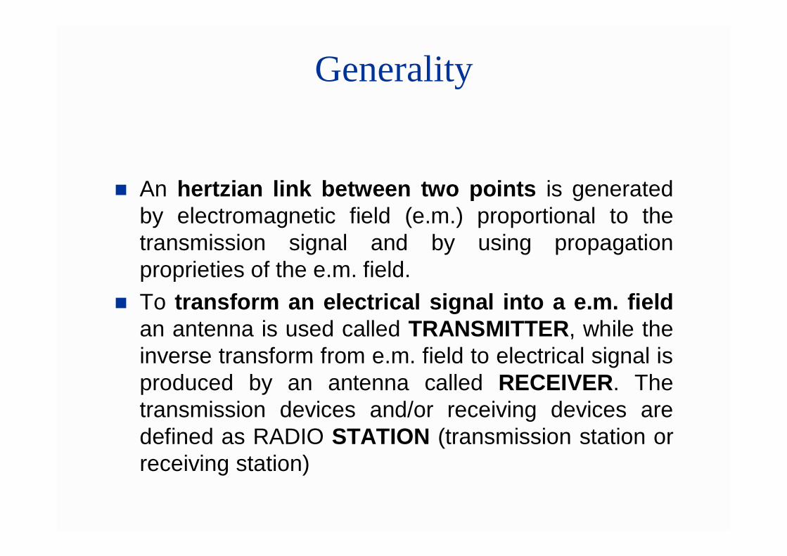
An hertzian link between two points is generatedby electromagnetic field (e.m.) proportional to thetransmission signal and by using propagationproprieties of the e.m. field.
To transform an electrical signal into a e.m. fieldan antenna is used called TRANSMITTER, while theinverse transform from e.m. field to electrical signal isproduced by an antenna called RECEIVER. Thetransmission devices and/or receiving devices aredefined as RADIO STATION (transmission station orreceiving station)
Circuit model for hertzian link (1/5)
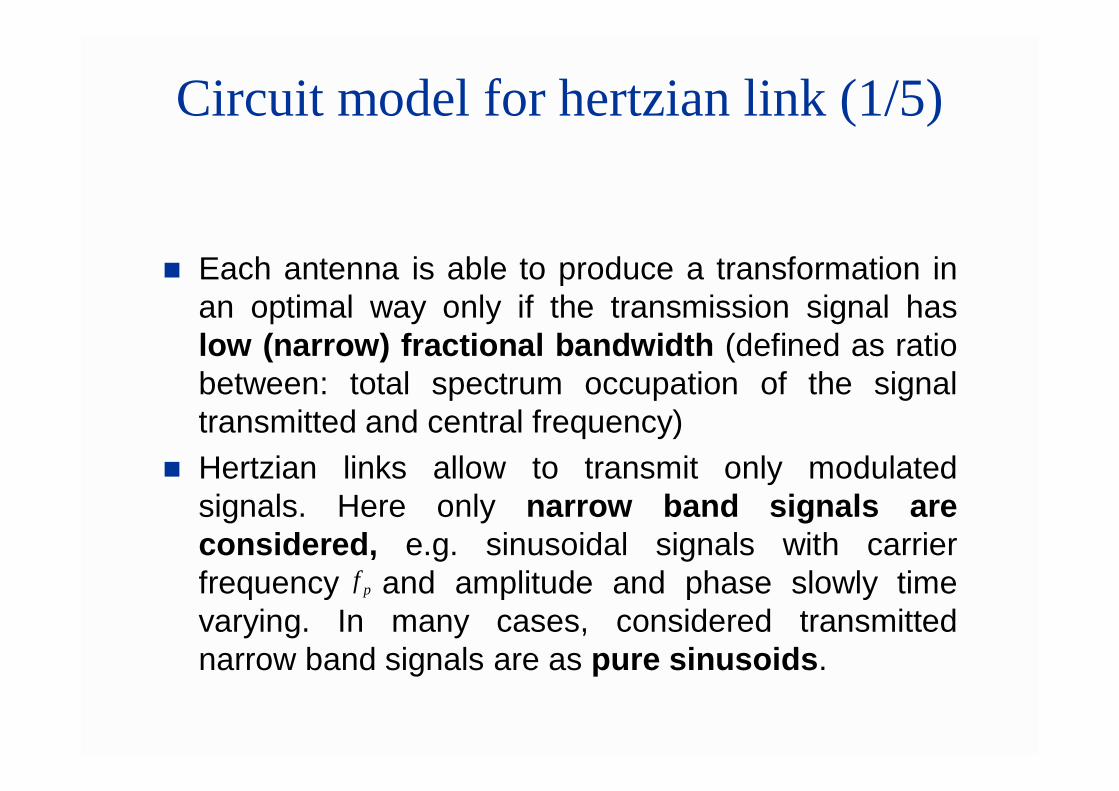
Each antenna is able to produce a transformation inan optimal way only if the transmission signal haslow (narrow) fractional bandwidth (defined as ratiobetween: total spectrum occupation of the signaltransmitted and central frequency)
Hertzian links allow to transmit only modulatedsignals. Here only narrow band signals areconsidered, e.g. sinusoidal signals with carrierfrequency and amplitude and phase slowly timevarying. In many cases, considered transmittednarrow band signals are as pure sinusoids.
pf
Circuit model for hertzian link (2/5)
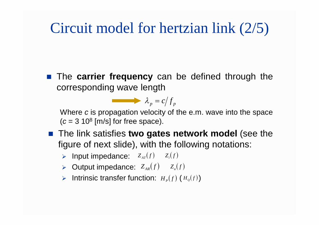
The carrier frequency can be defined through thecorresponding wave length
Where c is propagation velocity of the e.m. wave into the space(c = 3 108 [m/s] for free space).
The link satisfies two gates network model (see thefigure of next slide), with the following notations: Input impedance: Output impedance: Intrinsic transfer function: ( )
pp fc
fZ AT fZ i
fZ AR fZu
fH P fHQ
Circuit model for hertzian link (3/5)
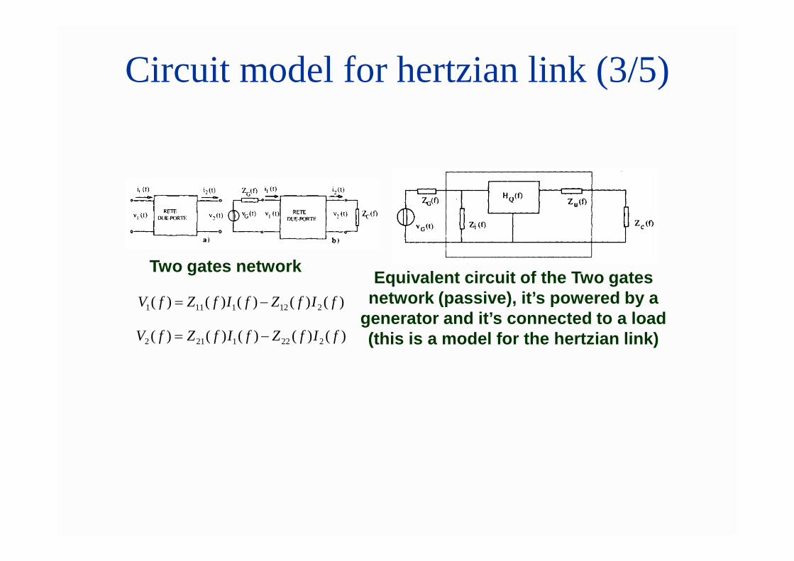
Two gates network Equivalent circuit of the Two gates network (passive), it’s powered by a
generator and it’s connected to a load (this is a model for the hertzian link)
)()()()()( 2121111 fIfZfIfZfV
)()()()()( 2221212 fIfZfIfZfV
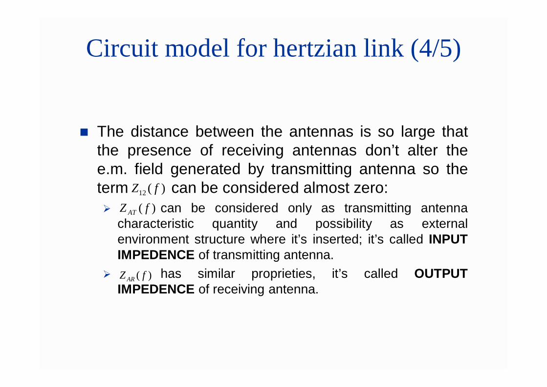
Circuit model for hertzian link (4/5)
The distance between the antennas is so large thatthe presence of receiving antennas don’t alter thee.m. field generated by transmitting antenna so theterm can be considered almost zero: can be considered only as transmitting antenna
characteristic quantity and possibility as externalenvironment structure where it’s inserted; it’s called INPUTIMPEDENCE of transmitting antenna.
has similar proprieties, it’s called OUTPUTIMPEDENCE of receiving antenna.
)(12 fZ)( fZ AT
)( fZ AR
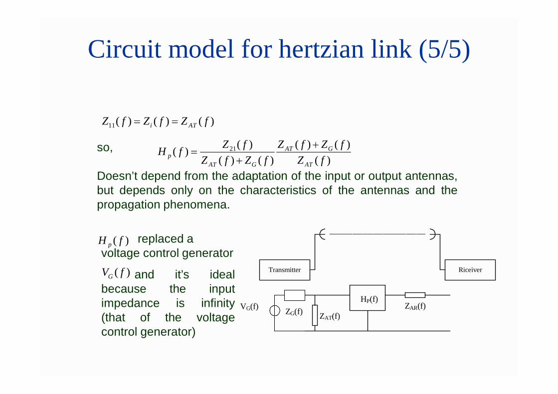
Circuit model for hertzian link (5/5)
HP(f)
ZAT(f) ZAR(f)
Transmitter Riceiver
ZG(f) VG(f)
so,
Doesn’t depend from the adaptation of the input or output antennas,but depends only on the characteristics of the antennas and thepropagation phenomena.
)()()(11 fZfZfZ ATi
)()()(
)()()()( 21
fZfZfZ
fZfZfZfH
AT
GAT
GATp
replaced a voltage control generator
and it’s idealbecause the inputimpedance is infinity(that of the voltagecontrol generator)
)( fH p
)( fVG
Characteristics of ideal free space hertzian link
Hypothesis: There aren’t other objects in the space. The space is isotropic and no-dissipative. The links between the antennas and the receiver are
adaptive to maximum power transfer (the output impedancesof the transmitter and input impedances of the receiver mustbe equal to and respectively into thebandwidth signal in transit.
Can be assumed that the hertzian link involves as perfect(ideal) channel, that introduces: Delay for finite speed of the e.m. field. Loss (amplitude reduction).
)(* fZAT
)(* fZAR
Types of antennas (1/2)
There are two basic of types of antennas: Isotropic antenna: this is ideal antenna, it radiates power
uniformly in all direction. Directional antenna: it doesn’t radiate power in uniformly
in the space, but it radiates greater (or lesser) power infunction of the direction. The antennas used in realapplication are directional
Types of antennas (2/2)
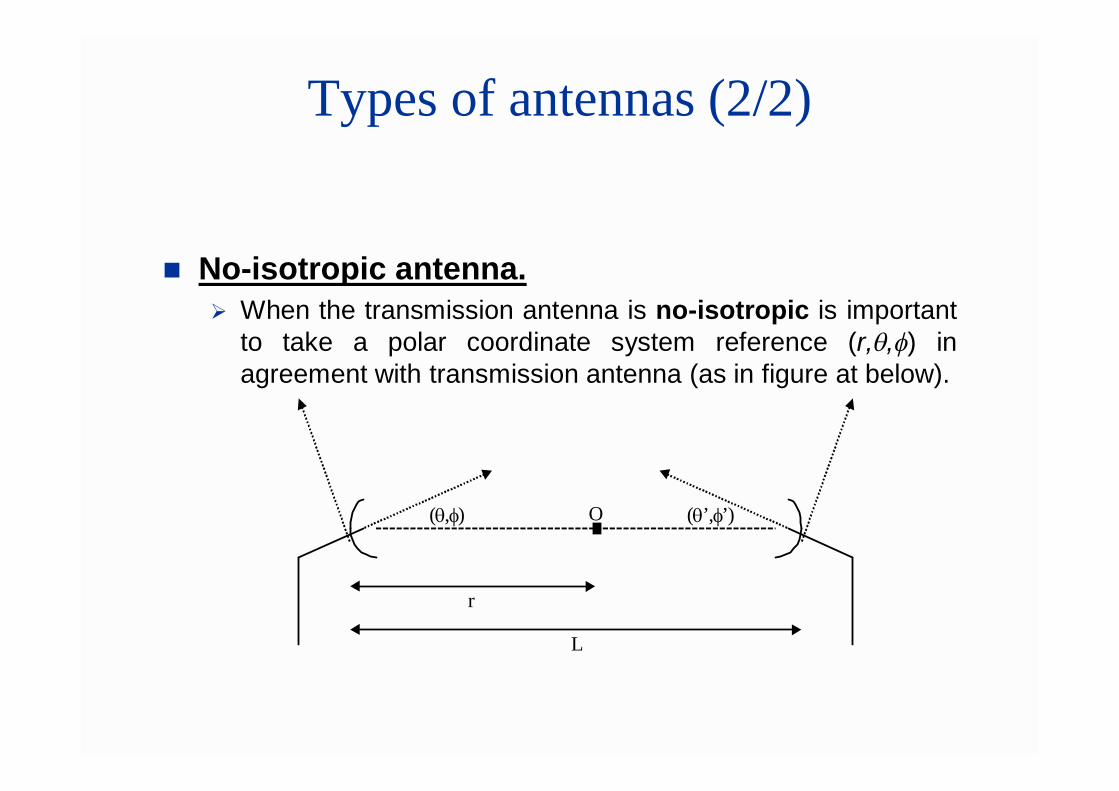
No-isotropic antenna. When the transmission antenna is no-isotropic is important
to take a polar coordinate system reference (r,q,f) inagreement with transmission antenna (as in figure at below).
O
L
r
(,) (’,’)
Antenna Gain (1/2)
It’s a parameter depends to physical characteristics of theantenna, in particular from the directionality.
Gain function GT(q,f ) is defined as a ratio betweenradiated power (or receive power) for solid angle unitfrom a directional antenna (take a given direction) andthe radiation power (or receive power) for solid angleunit from a isotropic antenna.
Antenna gain (Gmax) means the maximum value of thegain function, so the value at the direction of maximumradiation (generally it corresponds with theelectromagnetic axis of the antenna).
The gain antenna value is GT=1 for isotropic antenna.
Antenna Gain (2/2)
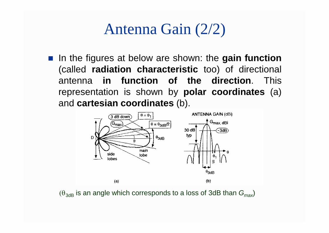
In the figures at below are shown: the gain function(called radiation characteristic too) of directionalantenna in function of the direction. Thisrepresentation is shown by polar coordinates (a)and cartesian coordinates (b).
3dB is an angle which corresponds to a loss of 3dB than Gmax)
Radiated power (1/6)
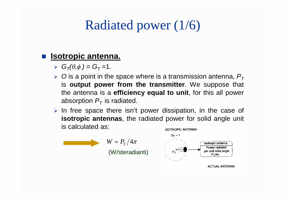
Isotropic antenna. GT(q,f ) = GT =1. O is a point in the space where is a transmission antenna, PT
is output power from the transmitter. We suppose thatthe antenna is a efficiency equal to unit, for this all powerabsorption PT is radiated.
In free space there isn’t power dissipation, in the case ofisotropic antennas, the radiated power for solid angle unitis calculated as:
4TPW
(W/steradianti)
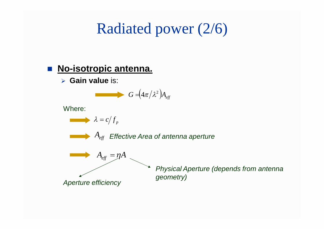
Radiated power (2/6)
No-isotropic antenna. Gain value is:
effAG 24
Where:
pfc
effA Effective Area of antenna aperture
AAeff
Physical Aperture (depends from antenna geometry)
Aperture efficiency
Radiated power (3/6)
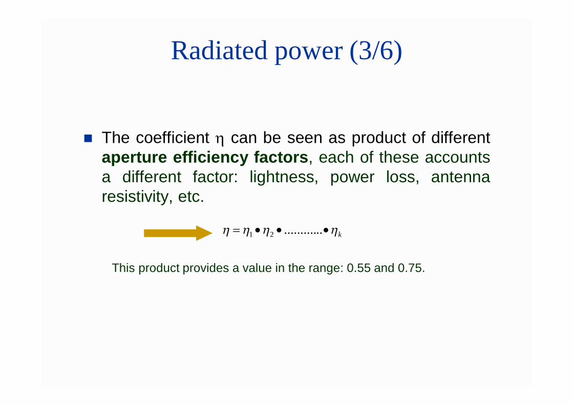
The coefficient h can be seen as product of differentaperture efficiency factors, each of these accountsa different factor: lightness, power loss, antennaresistivity, etc.
k ............21
This product provides a value in the range: 0.55 and 0.75.
Radiated power (4/6)
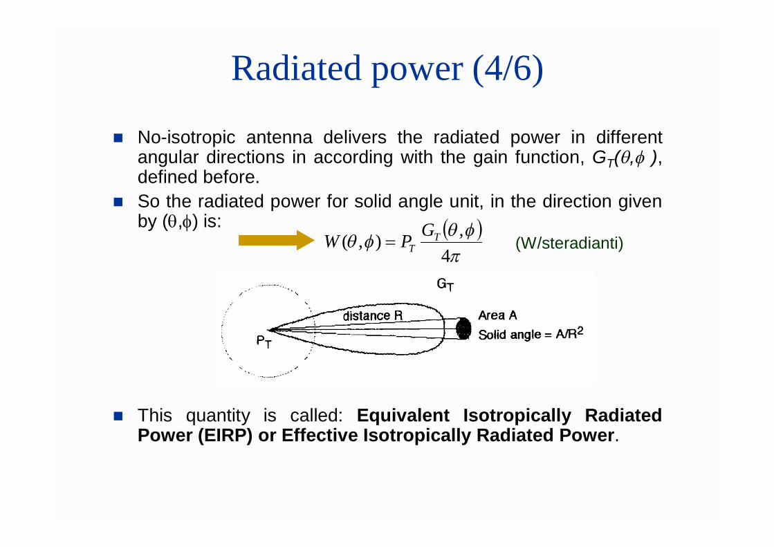
No-isotropic antenna delivers the radiated power in differentangular directions in according with the gain function, GT(q,f ),defined before.
So the radiated power for solid angle unit, in the direction givenby (,) is:
This quantity is called: Equivalent Isotropically RadiatedPower (EIRP) or Effective Isotropically Radiated Power.
fqfq
4,),( T
TGPW (W/steradianti)
Radiated power (5/6)
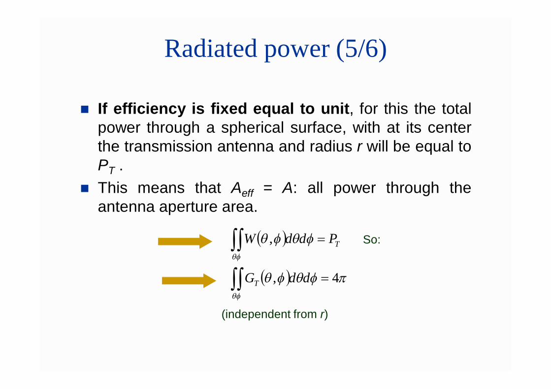
If efficiency is fixed equal to unit, for this the totalpower through a spherical surface, with at its centerthe transmission antenna and radius r will be equal toPT .
This means that Aeff = A: all power through theantenna aperture area.
fqfqqf
4, ddGT
TPddW fqfqqf
, So:
(independent from r)
Radiated power (6/6)
For the antenna gain given, the gain function GT(.,.)(ratio between radiated power from the directionalantenna and radiated power from isotropical antenna)will take values in the range 0 and Gmax.
An antenna is called directive if in a direction given(,), the gain function will take a maximum valuemuch greater than 1.
This maximum value, indicated with Gmax, is theANTENNA GAIN, already define before.
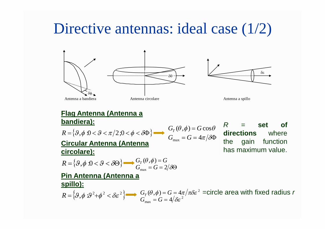
Directive antennas: ideal case (1/2)
Antenna a bandiera Antenna circolare Antenna a spillo
R = set ofdirections wherethe gain functionhas maximum value.
ff 0;20:,R 4max GG
f 0:,R 2max GG
222:, ff R 2max 4 GG
qfq cos),( GGT
GGT ),( fq
24),( fq GGT
Flag Antenna (Antenna a bandiera):
Circular Antenna (Antenna circolare):
Pin Antenna (Antenna a spillo):
=circle area with fixed radius r
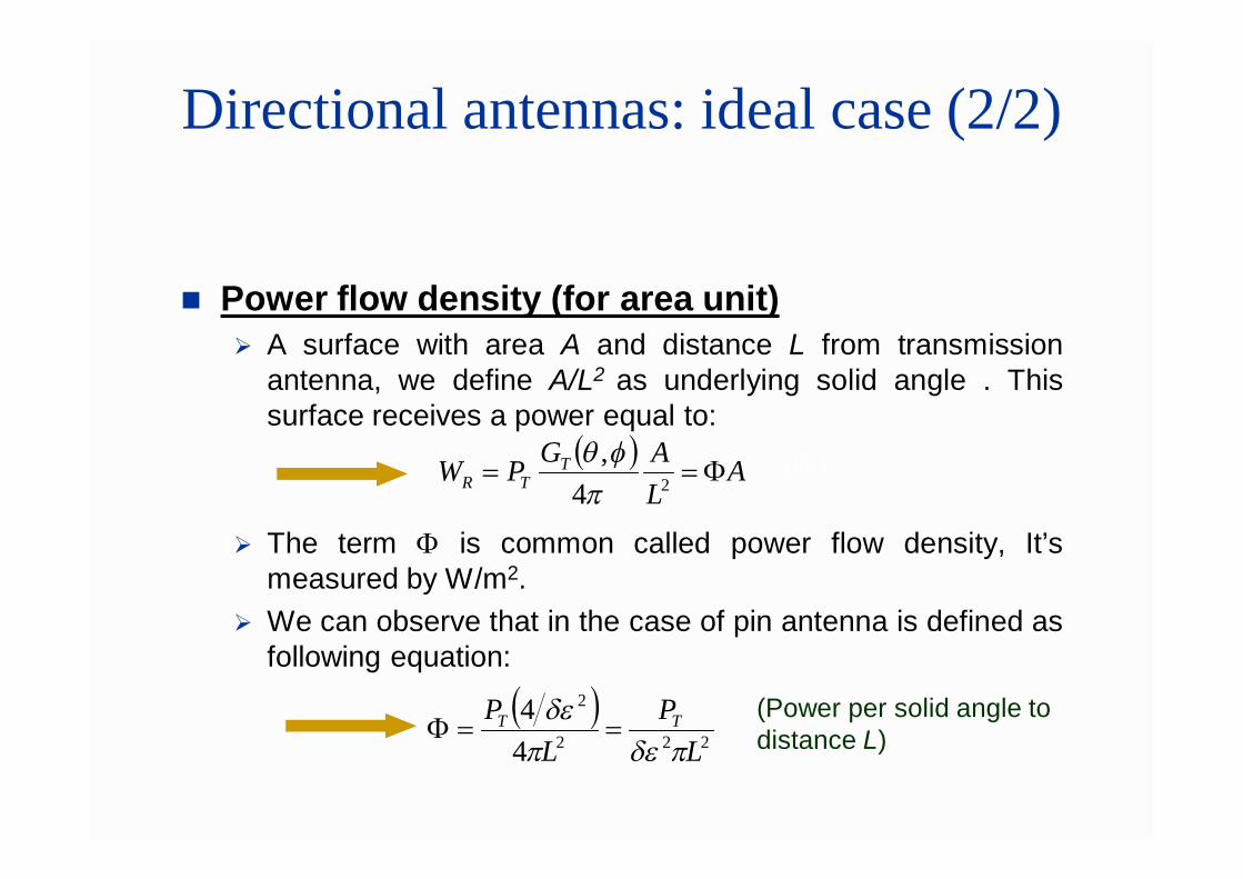
Directional antennas: ideal case (2/2)
Power flow density (for area unit) A surface with area A and distance L from transmission
antenna, we define A/L2 as underlying solid angle . Thissurface receives a power equal to:
The term is common called power flow density, It’smeasured by W/m2.
We can observe that in the case of pin antenna is defined asfollowing equation:
ALAGPW T
TR 24,fq (W)
222
2
44
LP
LP TT
(Power per solid angle to distance L)
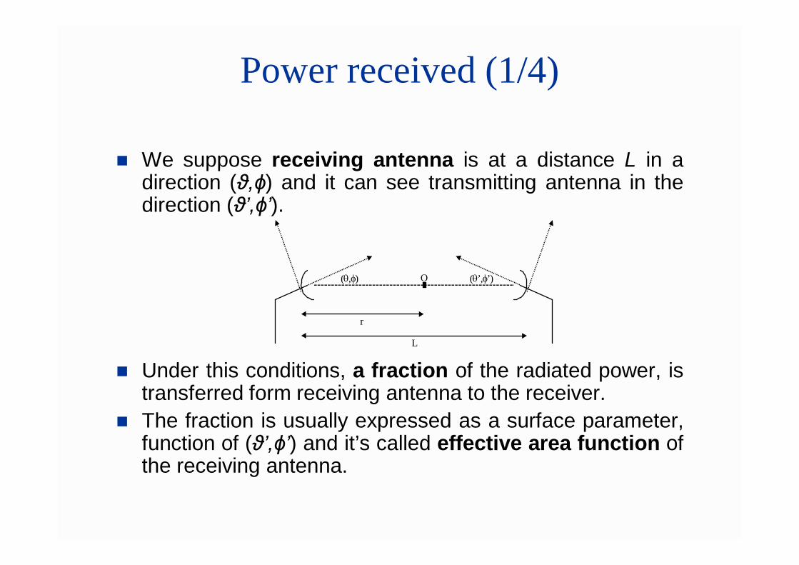
Power received (1/4)
We suppose receiving antenna is at a distance L in adirection (ϑ,ϕ) and it can see transmitting antenna in thedirection (ϑ’,ϕ’).
Under this conditions, a fraction of the radiated power, istransferred form receiving antenna to the receiver.
The fraction is usually expressed as a surface parameter,function of (ϑ’,ϕ’) and it’s called effective area function ofthe receiving antenna.
O
L
r
(,) (’,’)
Power received (2/4)
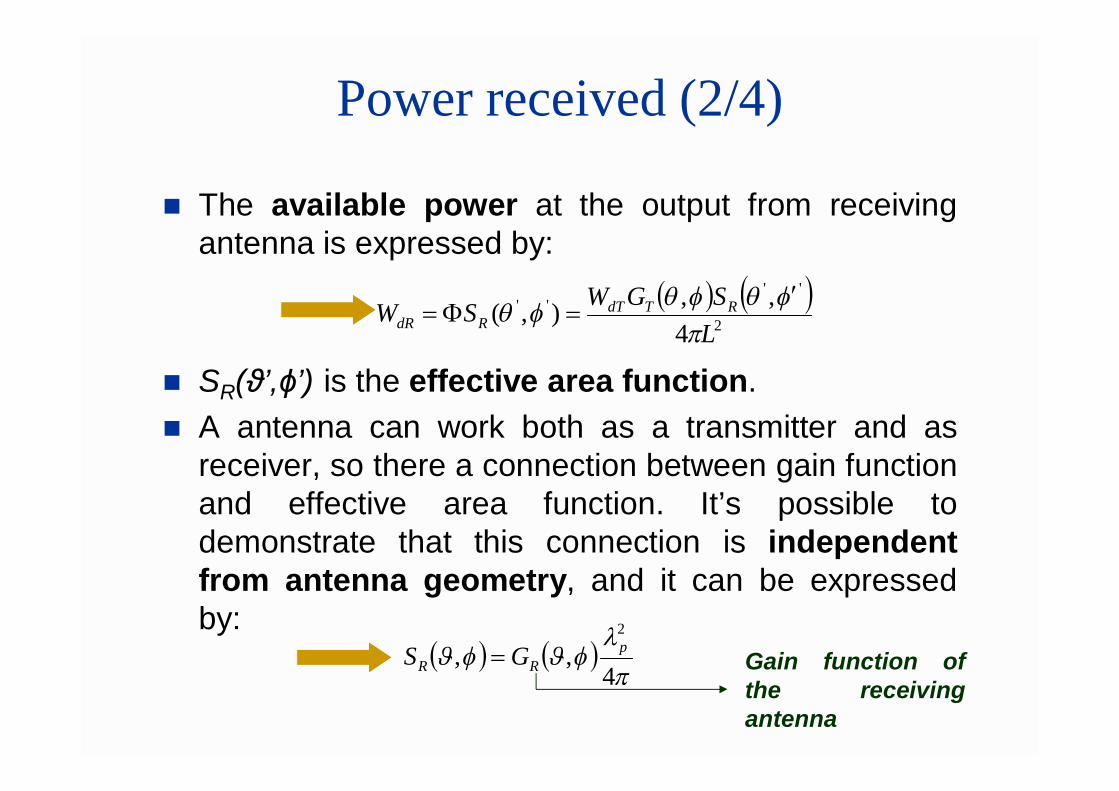
The available power at the output from receivingantenna is expressed by:
SR(ϑ’,ϕ’) is the effective area function. A antenna can work both as a transmitter and as
receiver, so there a connection between gain functionand effective area function. It’s possible todemonstrate that this connection is independentfrom antenna geometry, and it can be expressedby:
2
''''
4,,),(
LSGWSW RTdT
RdR fqfqfq
ff4
,,2p
RR GS Gain function ofthe receivingantenna
Power received (3/4)
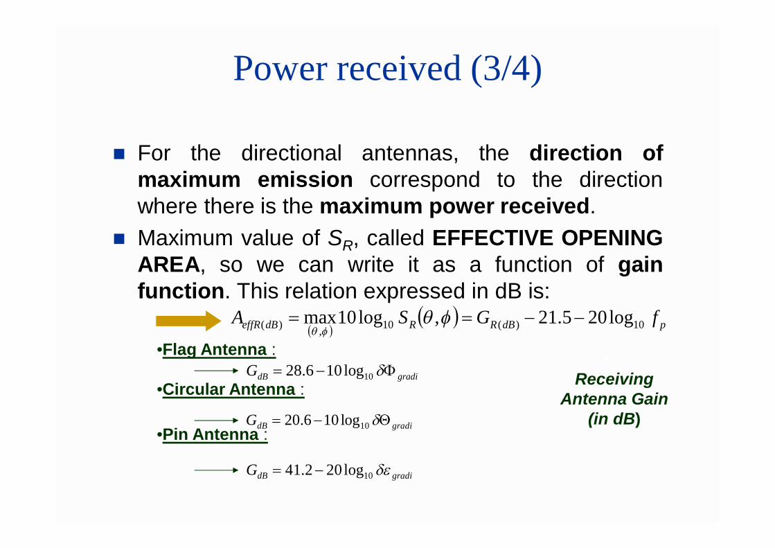
For the directional antennas, the direction ofmaximum emission correspond to the directionwhere there is the maximum power received.
Maximum value of SR, called EFFECTIVE OPENINGAREA, so we can write it as a function of gainfunction. This relation expressed in dB is:
•Flag Antenna :
•Circular Antenna :
•Pin Antenna :
gradidBG 10log106.28
gradidBG 10log106.20
gradidBG 10log202.41
Receiving Antenna Gain
(in dB)
pdBRRdBeffR fGSA 10)(10,)( log205.21,log10max fq
fq
Power received (4/4)
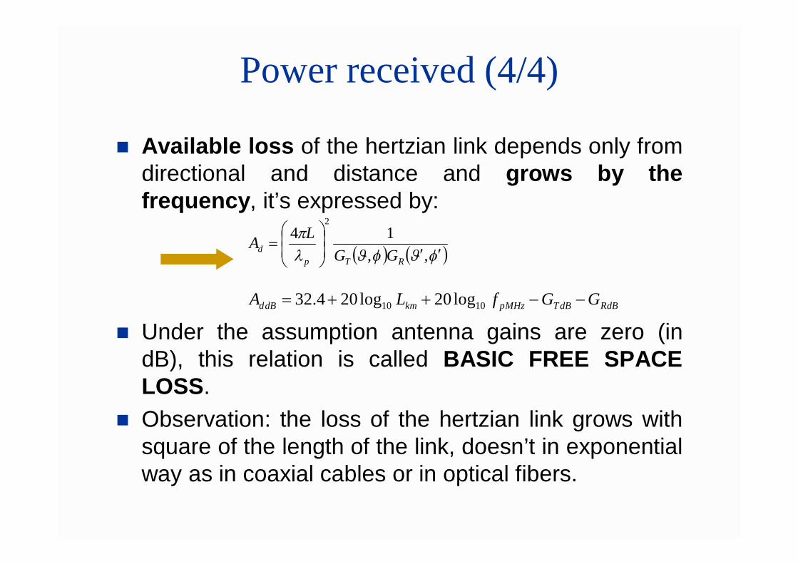
Available loss of the hertzian link depends only fromdirectional and distance and grows by thefrequency, it’s expressed by:
Under the assumption antenna gains are zero (indB), this relation is called BASIC FREE SPACELOSS.
Observation: the loss of the hertzian link grows withsquare of the length of the link, doesn’t in exponentialway as in coaxial cables or in optical fibers.
ff
,,14
2
RTpd GG
LA
dBRdBTMHzpkmdBd GGfLA 1010 log20log204.32
Worsening factors of a real link(1/2)
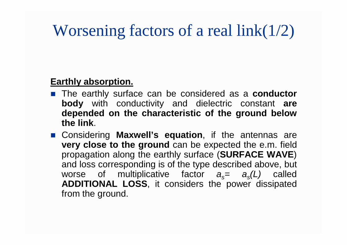
Earthly absorption. The earthly surface can be considered as a conductor
body with conductivity and dielectric constant aredepended on the characteristic of the ground belowthe link.
Considering Maxwell’s equation, if the antennas arevery close to the ground can be expected the e.m. fieldpropagation along the earthly surface (SURFACE WAVE)and loss corresponding is of the type described above, butworse of multiplicative factor as= as(L) calledADDITIONAL LOSS, it considers the power dissipatedfrom the ground.
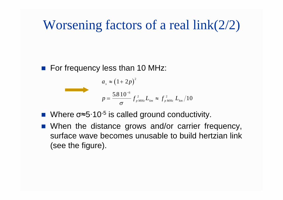
Worsening factors of a real link(2/2)
For frequency less than 10 MHz:
Where σ≈5∙10-5 is called ground conductivity. When the distance grows and/or carrier frequency,
surface wave becomes unusable to build hertzian link(see the figure).
a ps 1 2 2
p f L f Lp MHz km p MHz km 5 810 10
62 2.
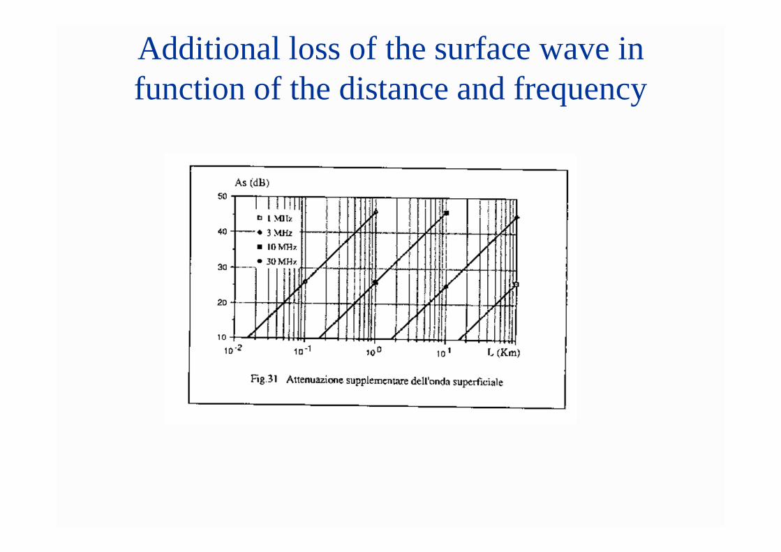
Additional loss of the surface wave in function of the distance and frequency
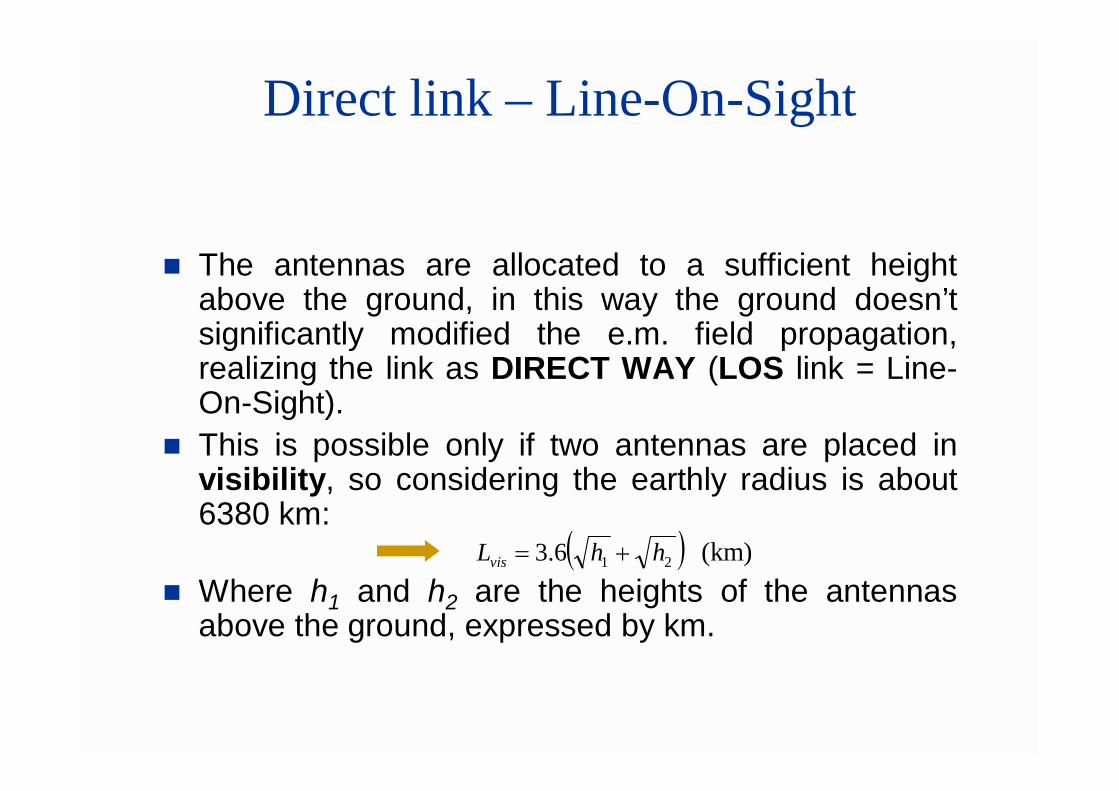
Direct link – Line-On-Sight
The antennas are allocated to a sufficient heightabove the ground, in this way the ground doesn’tsignificantly modified the e.m. field propagation,realizing the link as DIRECT WAY (LOS link = Line-On-Sight).
This is possible only if two antennas are placed invisibility, so considering the earthly radius is about6380 km:
(km) Where h1 and h2 are the heights of the antennas
above the ground, expressed by km.
216.3 hhLvis
Link LOS
Atmospheric absorption and rain. The hypothesis of not-dissipative space is true up
to about 10 GHz: above, the loss is worsted by amultiplicative term (ADDITIONAL LOSS) it isoriginate from oxygen, water vapor and rain.
The additional loss depends on oxygen absorptionand it becomes sensible to carrier frequenciesabove to 30 GHz, it’s maximum at 60 GHz (20dB/km).
The water vapor absorption has a maximum valueat about 22 GHz (12dB/km).
Rain Absorption
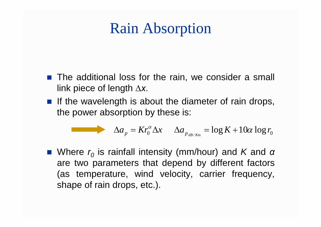
The additional loss for the rain, we consider a smalllink piece of length ∆x.
If the wavelength is about the diameter of rain drops,the power absorption by these is:
Where r0 is rainfall intensity (mm/hour) and K and αare two parameters that depend by different factors(as temperature, wind velocity, carrier frequency,shape of rain drops, etc.).
xKrap 0 0log10log
/rKa
KmdBp
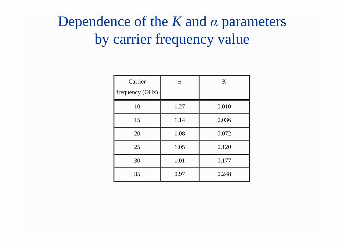
Dependence of the K and α parameters by carrier frequency value
Carrier
frequency (GHz)
K
10 1.27 0.010
15 1.14 0.036
20 1.08 0.072
25 1.05 0.120
30 1.01 0.177
35 0.97 0.248
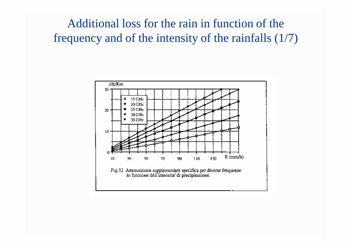
Additional loss for the rain in function of the frequency and of the intensity of the rainfalls (1/7)
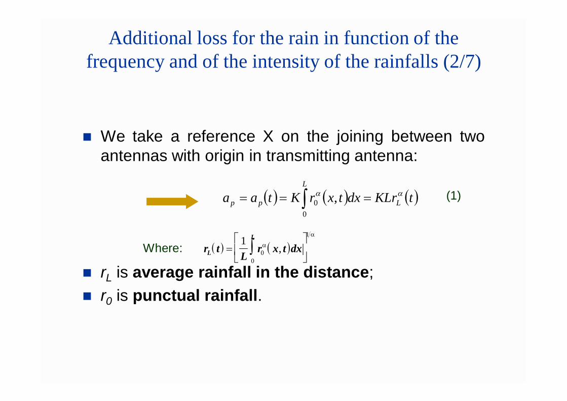
Additional loss for the rain in function of the frequency and of the intensity of the rainfalls (2/7)
We take a reference X on the joining between twoantennas with origin in transmitting antenna:
rL is average rainfall in the distance; r0 is punctual rainfall.
L
Lpp tKLrdxtxrKtaa0
0 ,
r tL
r x t dxL
L
1
00
1
,Where:
(1)
Additional loss for the rain in function of the frequency and of the intensity of the rainfalls (3/7)
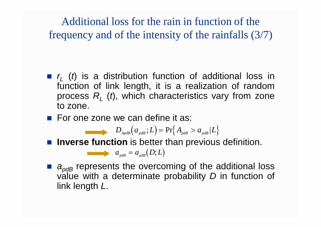
rL (t) is a distribution function of additional loss infunction of link length, it is a realization of randomprocess RL (t), which characteristics vary from zoneto zone.
For one zone we can define it as:
Inverse function is better than previous definition.
apdB represents the overcoming of the additional lossvalue with a determinate probability D in function oflink length L.
D a L A a LApdB pdB pdB pdB; Pr |
a a D LpdB pdB ;
Additional loss for the rain in function of the frequency and of the intensity of the rainfalls (4/7)
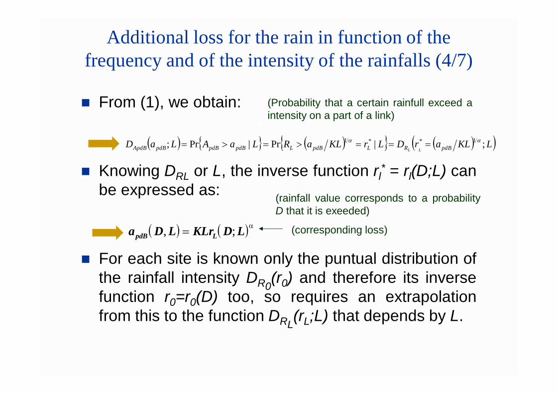
From (1), we obtain:
Knowing DRL or L, the inverse function rl* = rl(D;L) can
be expressed as:
For each site is known only the puntual distribution ofthe rainfall intensity DR0(r0) and therefore its inversefunction r0=r0(D) too, so requires an extrapolationfrom this to the function DRL(rL;L) that depends by L.
LKLarDLrKLaRLaALaD pdBRLpdBLpdBpdBpdBApdB LL;|Pr|Pr; 1**1
(Probability that a certain rainfull exceed aintensity on a part of a link)
a D L KLr D LpdB L, ;
(rainfall value corresponds to a probabilityD that it is exeeded)
(corresponding loss)
Additional loss for the rain in function of the frequency and of the intensity of the rainfalls (5/7)
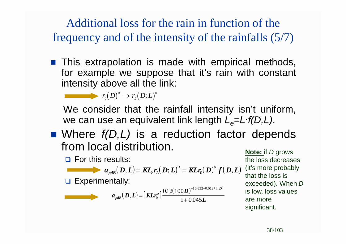
This extrapolation is made with empirical methods,for example we suppose that it’s rain with constantintensity above all the link:
We consider that the rainfall intensity isn’t uniform,we can use an equivalent link length Le=L∙f(D,L).
Where f(D,L) is a reduction factor dependsfrom local distribution. For this results:
Experimentally:
r D r D LL0
;
38/103
a D L KL r D L KLr D f D LpdB e L, ; , 0
a D L KLrD
LpdB
D
,.
.
. . ln
0
0 632 0 0187012 1001 0 045
Note: if D grows the loss decreases (it’s more probably that the loss is exceeded). When Dis low, loss values are more significant.
Additional loss for the rain in function of the frequency and of the intensity of the rainfalls (6/7)
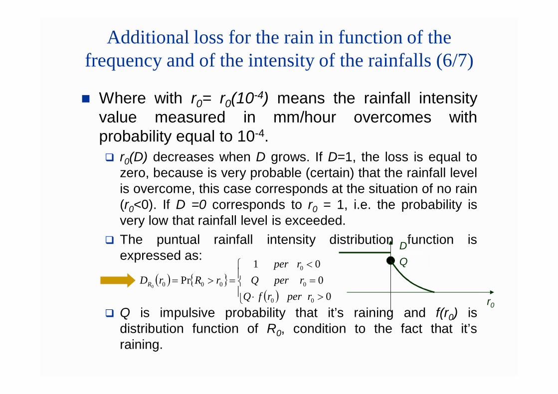
Where with r0= r0(10-4) means the rainfall intensityvalue measured in mm/hour overcomes withprobability equal to 10-4. r0(D) decreases when D grows. If D=1, the loss is equal to
zero, because is very probable (certain) that the rainfall levelis overcome, this case corresponds at the situation of no rain(r0<0). If D =0 corresponds to r0 = 1, i.e. the probability isvery low that rainfall level is exceeded.
The puntual rainfall intensity distribution function isexpressed as:
Q is impulsive probability that it’s raining and f(r0) isdistribution function of R0, condition to the fact that it’sraining.
0
0 0 1
Pr
00
0
0
0000
rperrfQrperQ
rperrRrDR
D
r0
Q
Additional loss for the rain in function of the frequency and of the intensity of the rainfalls (7/7)
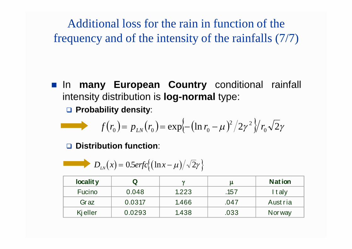
In many European Country conditional rainfallintensity distribution is log-normal type: Probability density:
Distribution function:
22lnexp 022
000 rrrprf LN
D x erfc xLN 0 5 2. ln
locality Q NationFucino 0.048 1.223 .157 ItalyGraz 0.0317 1.466 .047 Austria
Kjeller 0.0293 1.438 .033 Norway
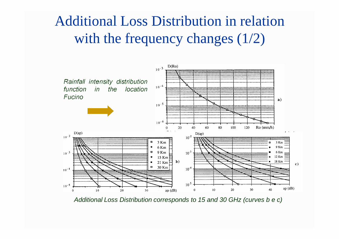
Additional Loss Distribution in relation with the frequency changes (1/2)
Rainfall intensity distributionfunction in the locationFucino
Additional Loss Distribution corresponds to 15 and 30 GHz (curves b e c)
Additional Loss Distribution in relation with the frequency changes (2/2)
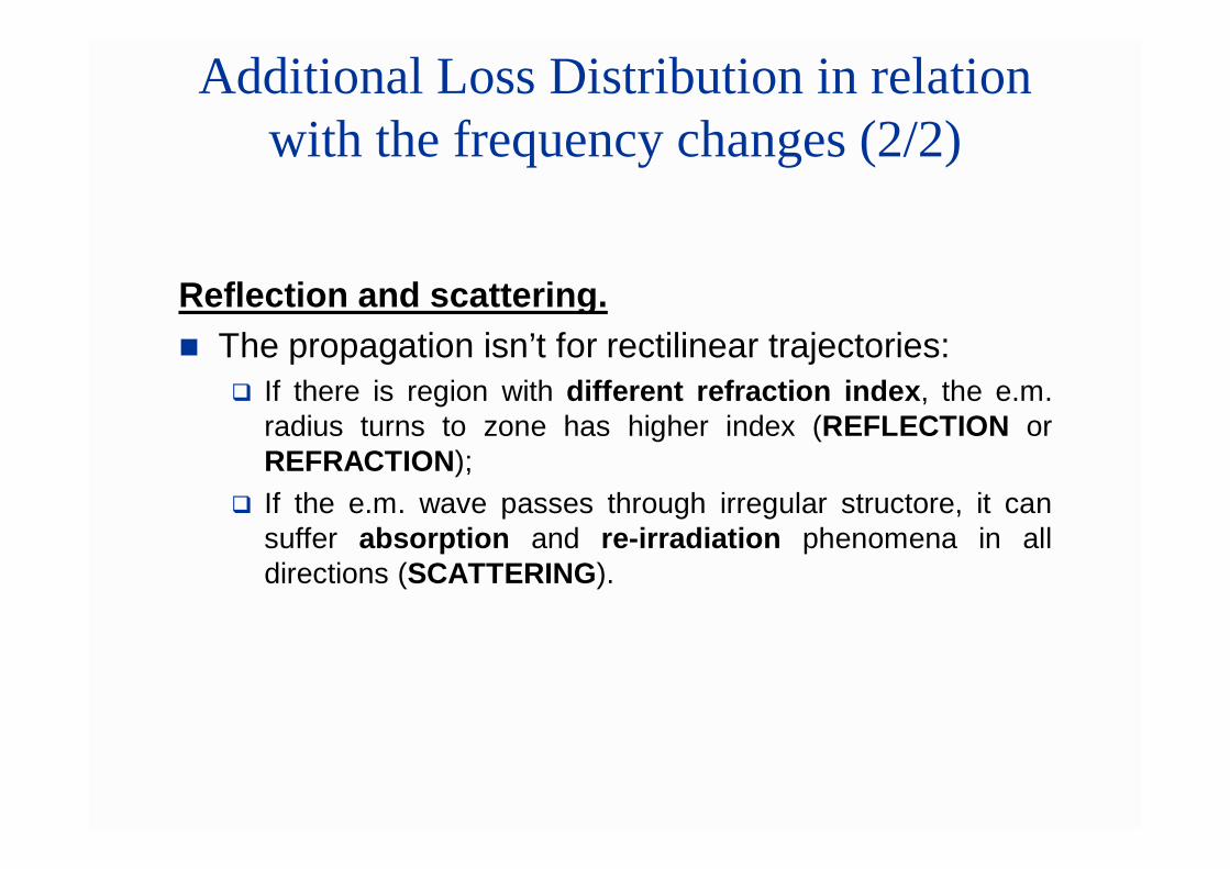
Reflection and scattering. The propagation isn’t for rectilinear trajectories:
If there is region with different refraction index, the e.m.radius turns to zone has higher index (REFLECTION orREFRACTION);
If the e.m. wave passes through irregular structore, it cansuffer absorption and re-irradiation phenomena in alldirections (SCATTERING).
Constitution of the atmosphere (1/3)
TROPOSPHERE is lower layer of the atmosphere, it extends toaltitude of about 20 km. refraction index can be variable, inparticular it decreases with altitude. It’s possible to havephenomena of scattering for frequencies between 100 MHzand 10 GHz.
IONOSPHERE is placed to altitude of about 80 km; the high concentration of electrons and free ions produce absorption and reflection phenomena for frequencies between 5 and 30 MHz.It’s possible identify the following layers: Layer D (50-90km), absorbing (daylight hours only); Layer E (110km), reflecting and quite stable; Layer F1 (220km), reflecting and quite stable; Layer F2 (300km), reflecting and quite stable; Layer E sporadic, reflecting.
Constitution of the atmosphere (2/3)
The ionosphere is involved by scattering phenomena,for frequencies from 35 to 50MHz, this is caused bythe presence of meteorites.
For carrier frequency value can occur the followingbehaviors: Between some tens of KHz to some MHz, the propagation
is by ground wave, with limited delivery capacity. Between some MHz to some tens of MHz, the propagation
is by direct beam (the delivery capacity is equal to optics),or by subsequent reflections on the E and F layers and onthe earthly surface, or by IONOSPHERIC SCATTERING.The link results extendible above the visibility, but it’s notperfect, because exist infinite path between the antennas.
Constitution of the atmosphere (3/3)
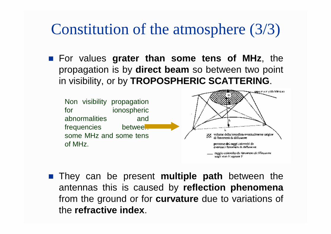
For values grater than some tens of MHz, thepropagation is by direct beam so between two pointin visibility, or by TROPOSPHERIC SCATTERING.
They can be present multiple path between theantennas this is caused by reflection phenomenafrom the ground or for curvature due to variations ofthe refractive index.
Non visibility propagationfor ionosphericabnormalities andfrequencies betweensome MHz and some tensof MHz.
Multiple paths
Each propagation anomalies, shown in previousslides, can be represented saying that the beams thatconnect between the antennas: Are more than one (MULTIPLE PATHS, called MULTIPLE
CHANNEL); Or this beams are infinite (TROPOSPHERIC SCATTERING
or IONOSPHERIC).
Notion on multiple paths
During the basic telecommunication courses, is beenconsidered the radio channel as Gaussian, additive, andwith limited bandwidth (AWGN channel).
This approximation can be accepted only few particularcases. Actually the propagations rules of the signals passthrough the ether are quite distant from a characterizationof the channel as AWGN channel.
The radio channel are characterized by multipathpropagation, that produces fading phenomena of thereceived signal. For this the radio channel is affected by aparticular distortion called multipath fading.
Time-varying impulse response
The AWGN channel is characterized by a time-invariantimpulse response, in the case of the Nyquist condition isrespected: the signaling rate is less than the double of thechannel bandwidth.
Instead a multipath channel is characterized by time-varying impulse response.
When very narrow impulse is transmitted (ideally a Diracdelta), the channel response will typically be a impulsetrain, spaced one to the other by time interval called timespread (t). Impulse amplitudes will be distorted (loss).
When transmission experiments are repeated at differenttimes both the time spread that the loss will take differentcharacteristics, as shown in the next slide.
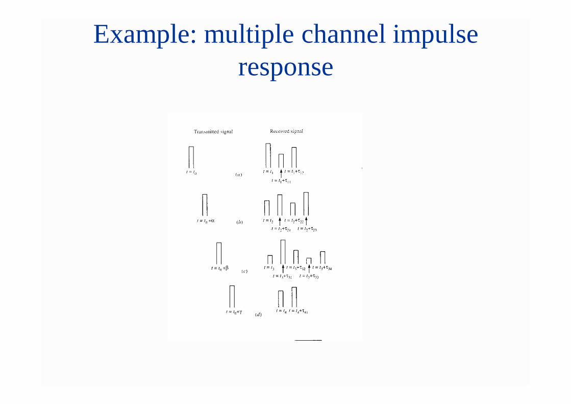
Example: multiple channel impulse response
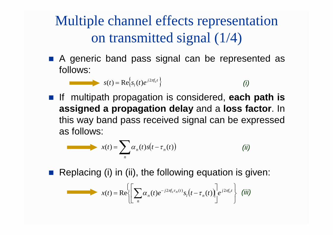
Multiple channel effects representation on transmitted signal (1/4)
A generic band pass signal can be represented asfollows:
If multipath propagation is considered, each path isassigned a propagation delay and a loss factor. Inthis way band pass received signal can be expressedas follows:
Replacing (i) in (ii), the following equation is given:
tfjl
cetsts 2)(Re)( (i)
n
nn ttsttx )()()( (ii)
tfj
nnl
tfjn
cnc ettsettx 2)(2 )()(Re)( (iii)
Multiple channel effects representation on transmitted signal (2/4)
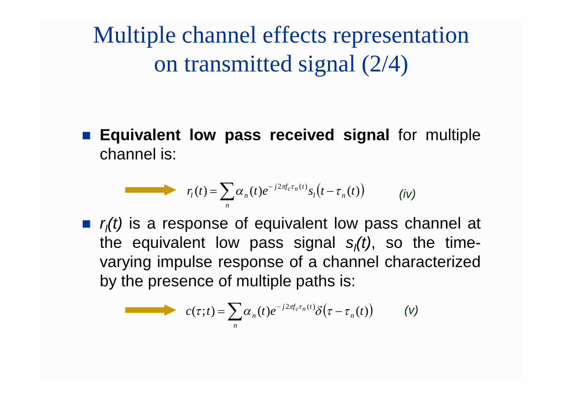
Equivalent low pass received signal for multiplechannel is:
rl(t) is a response of equivalent low pass channel atthe equivalent low pass signal sl(t), so the time-varying impulse response of a channel characterizedby the presence of multiple paths is:
nnl
tfjnl ttsettr nc )()()( )(2
(iv)
nn
tfjn tettc nc )()();( )(2 (v)
Multiple channel effects representation on transmitted signal (3/4)
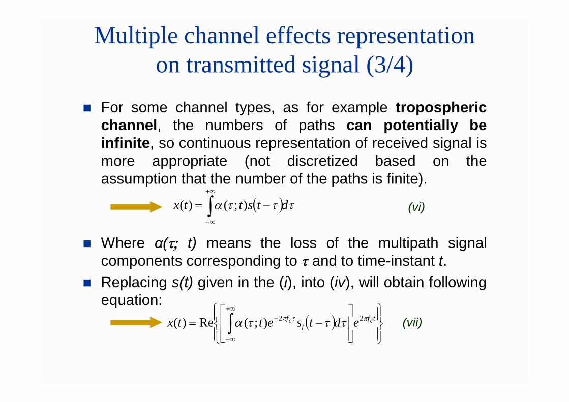
For some channel types, as for example troposphericchannel, the numbers of paths can potentially beinfinite, so continuous representation of received signal ismore appropriate (not discretized based on theassumption that the number of the paths is finite).
Where α(t; t) means the loss of the multipath signalcomponents corresponding to t and to time-instant t.
Replacing s(t) given in the (i), into (iv), will obtain followingequation:
dtsttx
);()( (vi)
tfl
f cc edtsettx 22);(Re)( (vii)
Multiple channel effects representation on transmitted signal (4/4)
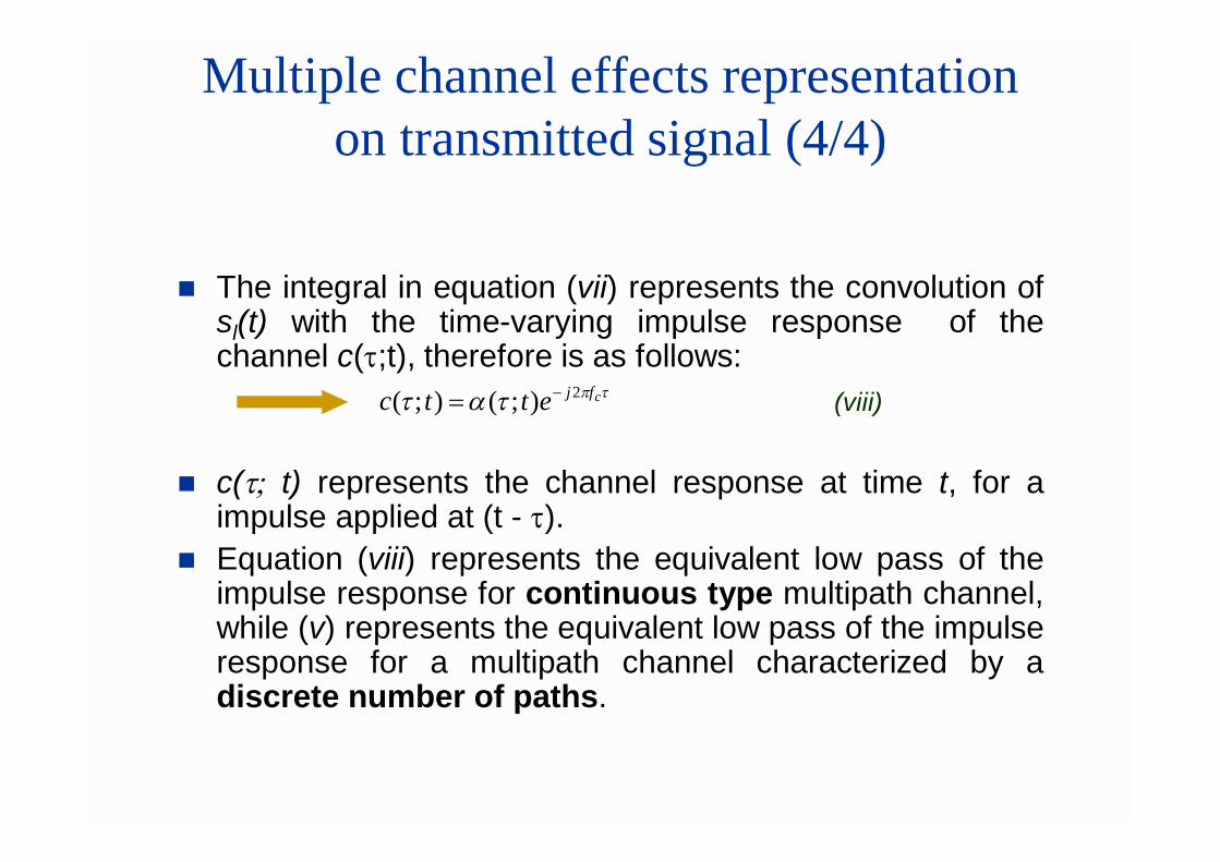
The integral in equation (vii) represents the convolution ofsl(t) with the time-varying impulse response of thechannel c(t;t), therefore is as follows:
c(; t) represents the channel response at time t, for aimpulse applied at (t - t).
Equation (viii) represents the equivalent low pass of theimpulse response for continuous type multipath channel,while (v) represents the equivalent low pass of the impulseresponse for a multipath channel characterized by adiscrete number of paths.
cfjettc 2);();( (viii)
Statistical multipath channel representation (1/4)
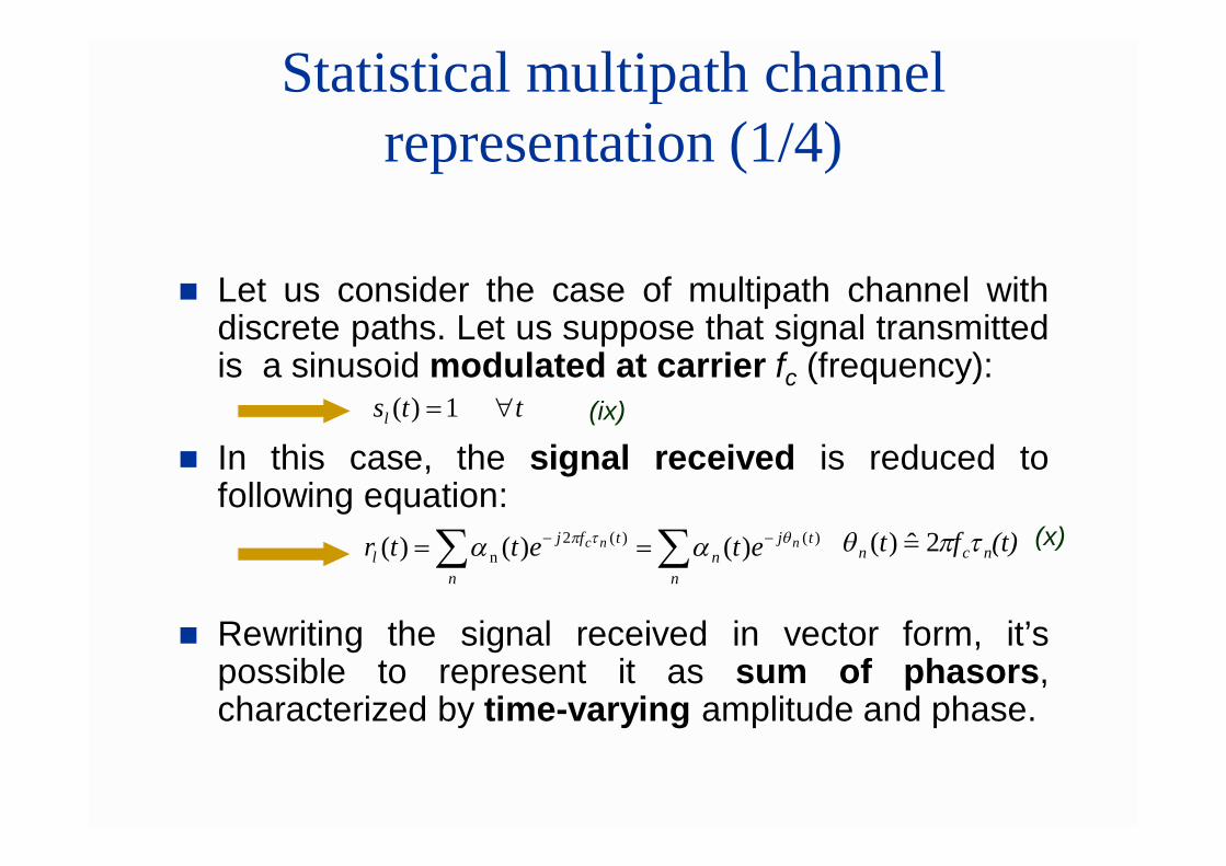
Let us consider the case of multipath channel withdiscrete paths. Let us suppose that signal transmittedis a sinusoid modulated at carrier fc (frequency):
In this case, the signal received is reduced tofollowing equation:
Rewriting the signal received in vector form, it’spossible to represent it as sum of phasors,characterized by time-varying amplitude and phase.
ttsl 1)( (ix)
)()()( )()(2n
n n
tjn
tfjl
nnc etettr q 2ˆ)( (t)ft ncn q (x)
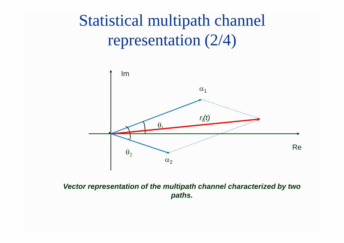
Statistical multipath channel representation (2/4)
Im
Re
1
2
2
1rl(t)
Vector representation of the multipath channel characterized by two paths.
Statistical multipath channel representation (3/4)
If the means used for the propagation is stable, n(t)value will suffer small oscillations over time.
But n(t) can vary by a factor of 2p if tn(t) varies by a factorof 1/fc, that generally is very small number.
Whereby n(t) is very sensible parameter for smalloscillations of the time-varying characteristic of themultipath channel.
Moreover we expect that propagation delay tn(t),associates to each path, varies in absolutelyunpredictable way (for this we consider this type ofpropagation as random process).
This fact means that received signal rl(t) can be modeledas random process.
Statistical multipath channel representation (4/4)
If the number of the paths is very high (as we canreasonably assume for real radio channels), it’s possibleto use the central limit theorem and we can suppose rl(t)as complex values Gaussian random process.
For this the multipath channel impulse response c( ; t)could be modeled as complex values Gaussian randomprocess.
Multipath propagation of real radio channels, represents inthe equation (x) can be translated to physic layer in afading phenomena of the received signal. Thisphenomena is known as multipath fading.
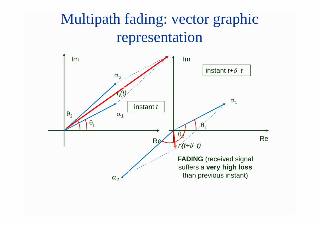
Multipath fading: vector graphic representation
Im
Re
1
2
21
rl(t)
instant t1
Im
Re
12
2
instant t+ t
rl(t+ t)
FADING (received signal suffers a very high loss
than previous instant)
Multipath fading effects on communication quality
From the graphics shown in the previous slide, themultipath fading causes many temporal fluctuations ofthe signal power received.
In practice: at subsequent time instants the signalsometime can be amplified (vector constructive effect ofthe multipath) or can be lessened (vector destructiveeffect of the multipath), all this caused by wide hiking ofthe time-varying phase shift value qn(t).
This effect can be observed, at macroscopic level (andanalogical level), for example when the signal is receivedfrom common car radio.
In digital system transmission, will observe significantincrease of BER at of “subsidence” of signal for multipathfading, for this it can be considered as self-interference.
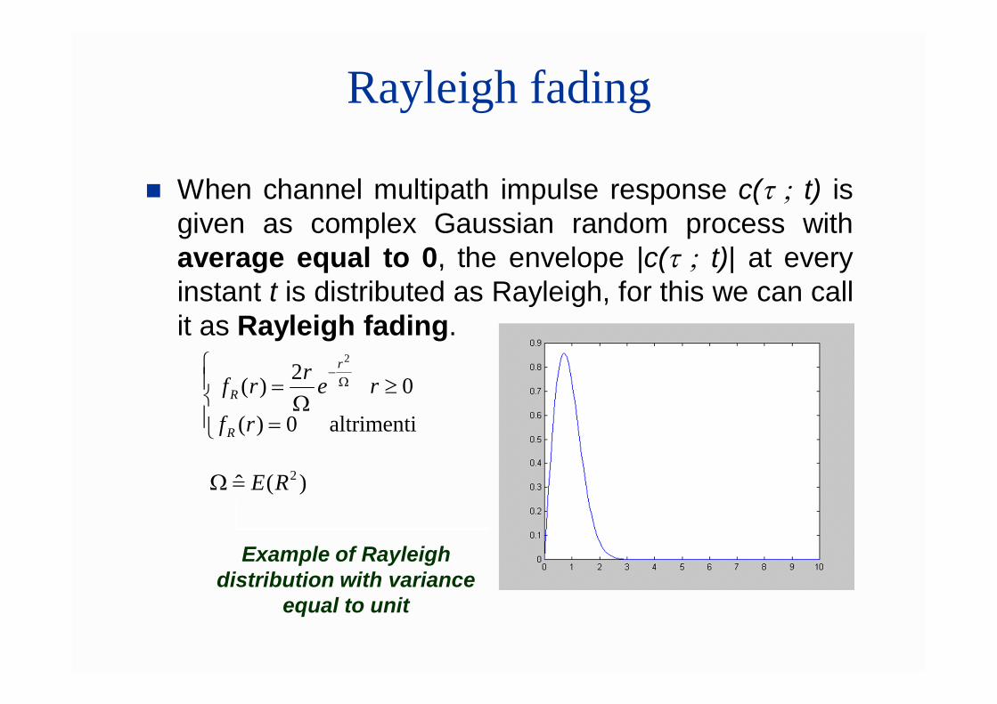
Rayleigh fading
When channel multipath impulse response c( ; t) isgiven as complex Gaussian random process withaverage equal to 0, the envelope |c( ; t)| at everyinstant t is distributed as Rayleigh, for this we can callit as Rayleigh fading.
altrimenti 0)(
0 2)(2
rf
rerrf
R
r
R
)(ˆ 2RE
Example of Rayleigh distribution with variance
equal to unit
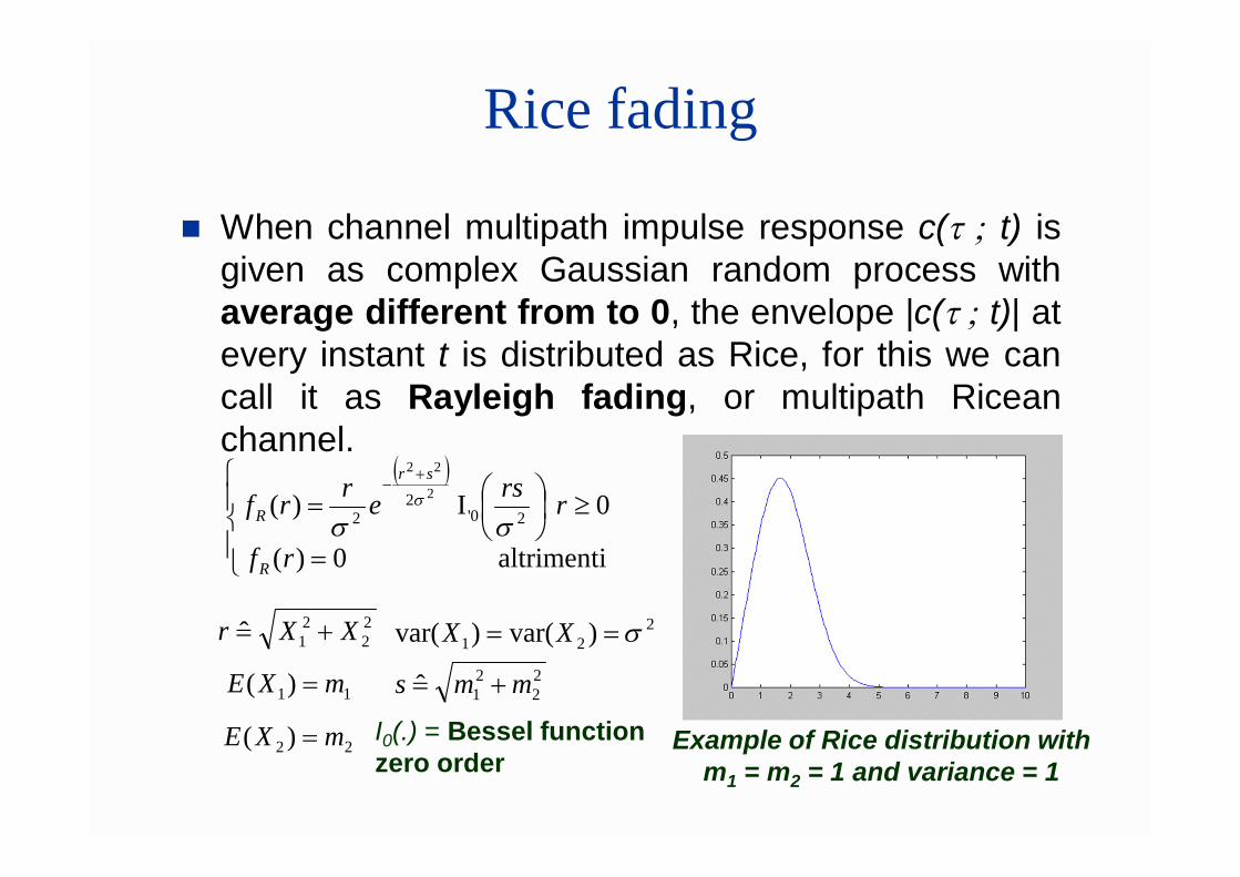
Rice fading
When channel multipath impulse response c( ; t) isgiven as complex Gaussian random process withaverage different from to 0, the envelope |c( ; t)| atevery instant t is distributed as Rice, for this we cancall it as Rayleigh fading, or multipath Riceanchannel.
altrimenti 0)(
0 I )( 2'02
22
22
rf
rrserrf
R
sr
R
22
21ˆ XXr
11)( mXE
22 )( mXE
221 )var()var( XX
22
21ˆ mms
I0(.) = Bessel function zero order
Example of Rice distribution with m1 = m2 = 1 and variance = 1
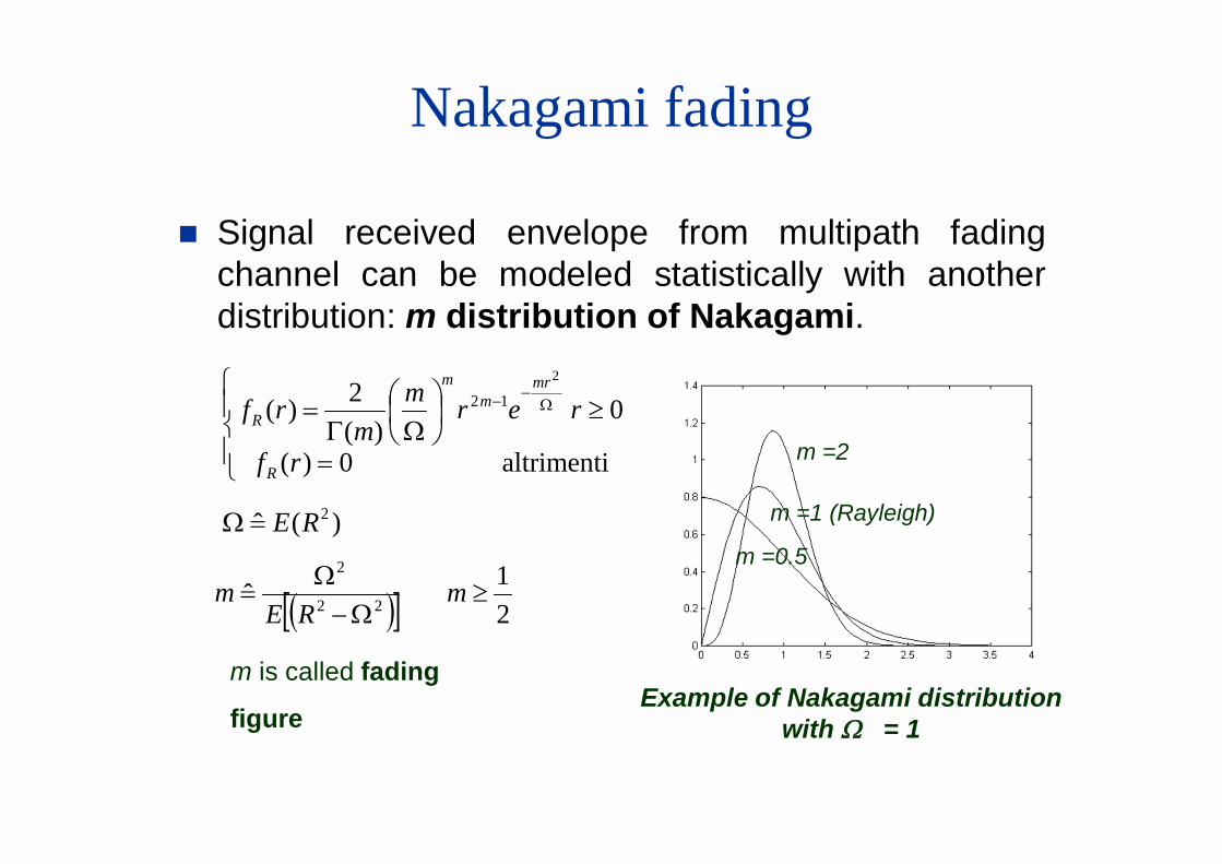
Nakagami fading
Signal received envelope from multipath fadingchannel can be modeled statistically with anotherdistribution: m distribution of Nakagami.
altrimenti 0)(
0 )(
2)(2
12
rf
rermm
rf
R
mrm
m
R
)(ˆ 2RE
21 ˆ 22
2
m
REm
m is called fading
figure
m =2
m =1 (Rayleigh)
m =0.5
Example of Nakagami distribution with W = 1
Use of different fading model (1/3)
The model of the Rayileigh fading is generally used in theradio-channel where doesn’t exist the line of sight (LOS) signalcomponent and desired signal is received only through itsreplicas, they can be delayed and phase shifted.
This situation mostly occurs in the case of radio channel,where the antennas are placed height lower than reflectionmeans and dispersion of the signal (tree, building).
The model of the Rice fading is useful in the cases of existenceof a LOS signal component, which is received with somereplicas delayed and phase shifted, these replicas aregenerated by secondary reflections of direct component.
These replicas are interfering pure signals.
Use of different fading model (2/3)
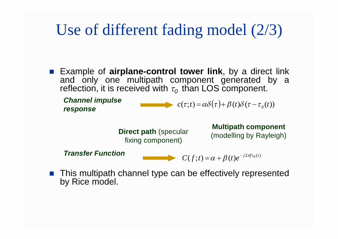
Example of airplane-control tower link, by a direct linkand only one multipath component generated by areflection, it is received with 0 than LOS component.
This multipath channel type can be effectively representedby Rice model.
))(()();( 0 tttc Channel impulse response
Multipath component (modelling by Rayleigh)
Transfer Function )(2 0)();( tfjettfC
Direct path (specular fixing component)
Use of different fading model (3/3)
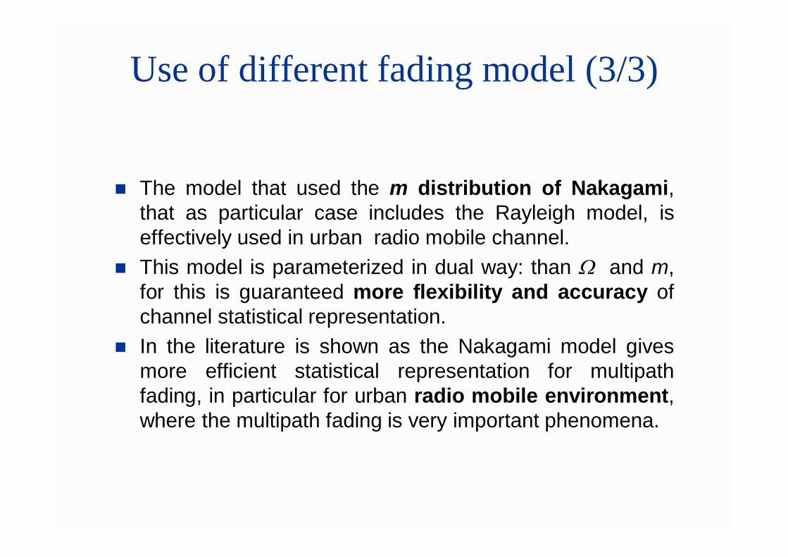
The model that used the m distribution of Nakagami,that as particular case includes the Rayleigh model, iseffectively used in urban radio mobile channel.
This model is parameterized in dual way: than W and m,for this is guaranteed more flexibility and accuracy ofchannel statistical representation.
In the literature is shown as the Nakagami model givesmore efficient statistical representation for multipathfading, in particular for urban radio mobile environment,where the multipath fading is very important phenomena.
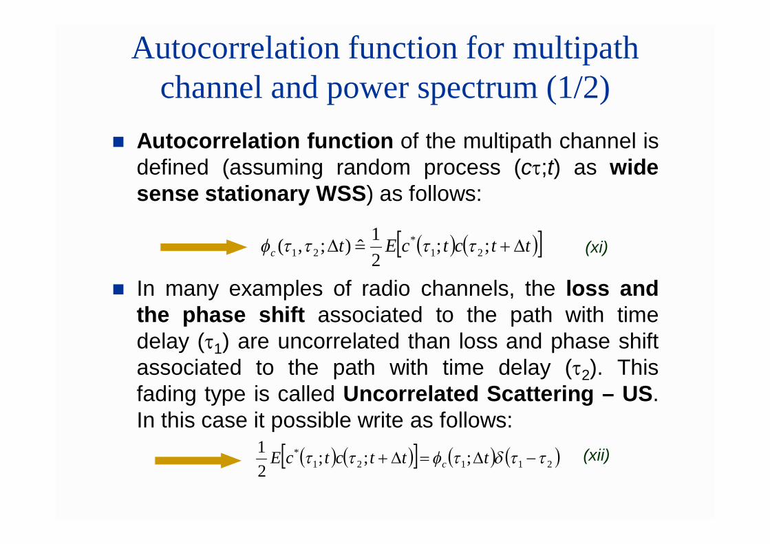
Autocorrelation function for multipath channel and power spectrum (1/2)
Autocorrelation function of the multipath channel isdefined (assuming random process (ct;t) as widesense stationary WSS) as follows:
In many examples of radio channels, the loss andthe phase shift associated to the path with timedelay (t1) are uncorrelated than loss and phase shiftassociated to the path with time delay (t2). Thisfading type is called Uncorrelated Scattering – US.In this case it possible write as follows:
ttctcEtc ;;21
ˆ);,( 21*
21 f (xi)
21121* ;;;
21 f tttctcE c
(xii)
Autocorrelation function for multipath channel and power spectrum (2/2)
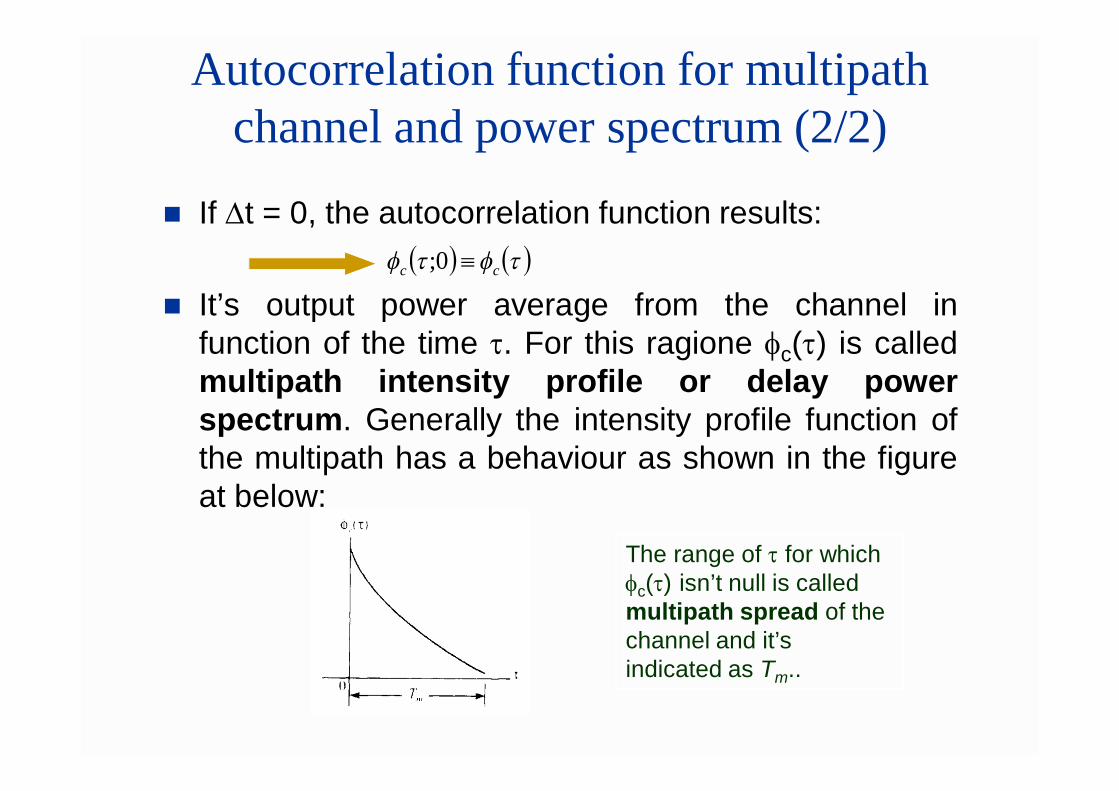
If t = 0, the autocorrelation function results:
It’s output power average from the channel infunction of the time t. For this ragione c(t) is calledmultipath intensity profile or delay powerspectrum. Generally the intensity profile function ofthe multipath has a behaviour as shown in the figureat below:
ff cc 0;
The range of t for which c(t) isn’t null is called multipath spread of the channel and it’s indicated as Tm..
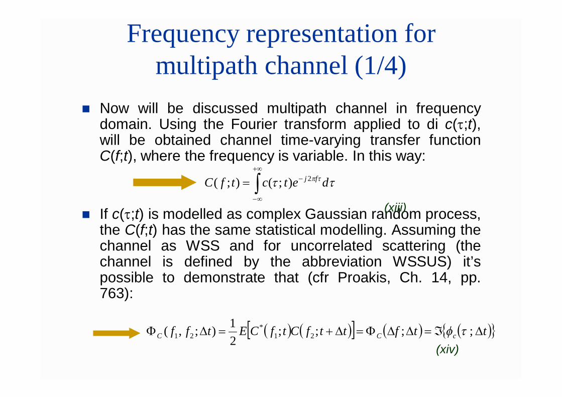
Frequency representation for multipath channel (1/4)
Now will be discussed multipath channel in frequencydomain. Using the Fourier transform applied to di c(t;t),will be obtained channel time-varying transfer functionC(f;t), where the frequency is variable. In this way:
If c(t;t) is modelled as complex Gaussian random process,the C(f;t) has the same statistical modelling. Assuming thechannel as WSS and for uncorrelated scattering (thechannel is defined by the abbreviation WSSUS) it’spossible to demonstrate that (cfr Proakis, Ch. 14, pp.763):
detctfC fj
2) ;();(
(xiii)
ttfttfCtfCEtff cCC ; ;;;21);,( 21
*21 f
(xiv)
Frequency representation for multipath channel (2/4)
In (xiv) is been placed f = f2 - f1 and we can note thatC(f,t) is the Fourier transform of the function fc(t;t),it gives output average power of the channel as function ofthe delay t and of the difference t between two observingtime instant (in t = 0 is multipath intensity profile).
The function C(f,t), is called channel correlationfunction spaced in time-frequency, and it can measuretransmitting a couple of sinusoids spaced between themof f and doing an operation of cross-correlation betweenthese two signal separately received with a delay t.
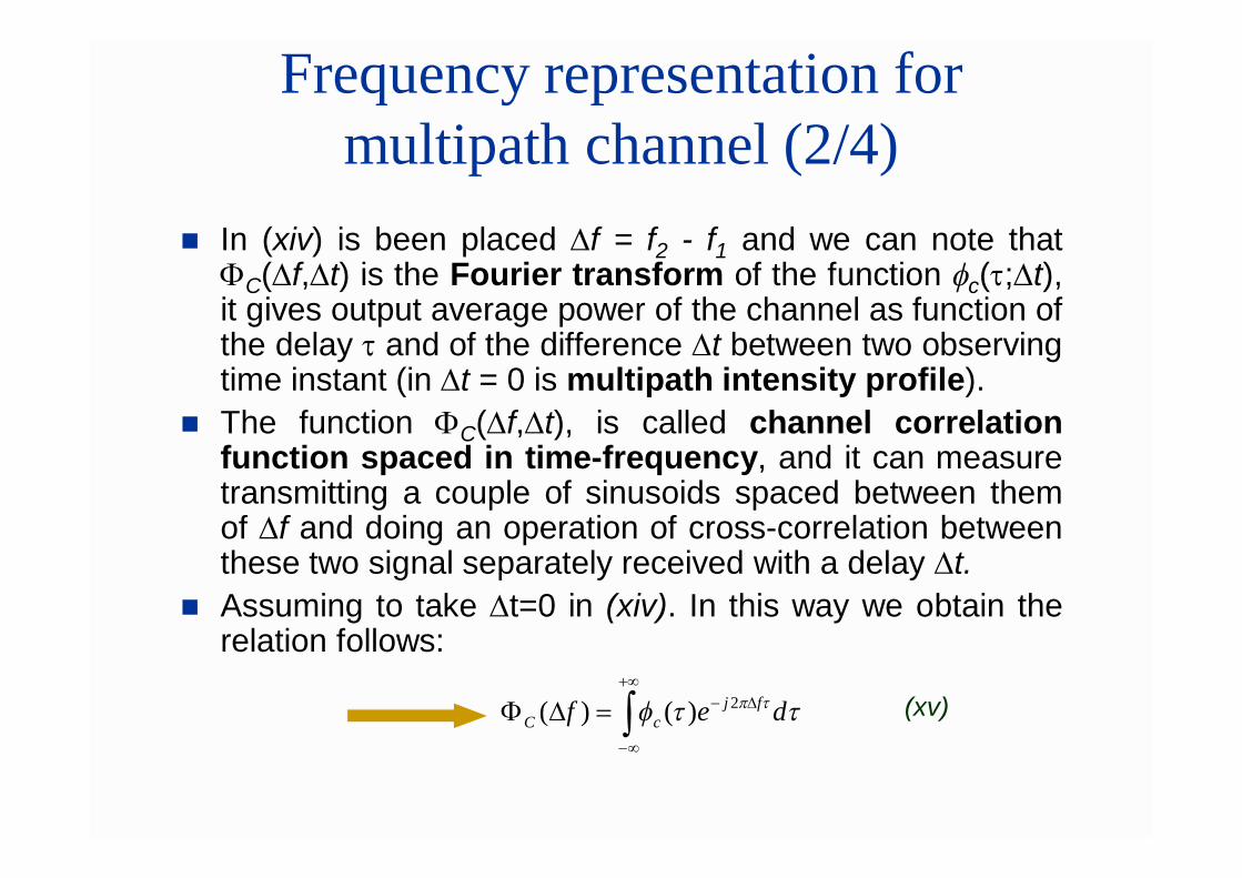
Assuming to take t=0 in (xiv). In this way we obtain therelation follows:
f def fjcC
2)()( (xv)
Frequency representation for multipath channel (3/4)
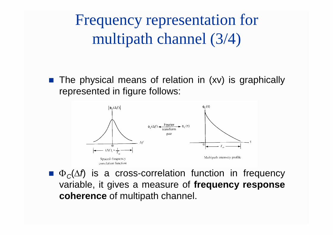
The physical means of relation in (xv) is graphicallyrepresented in figure follows:
C(f) is a cross-correlation function in frequencyvariable, it gives a measure of frequency responsecoherence of multipath channel.
Frequency representation for multipath channel (4/4)
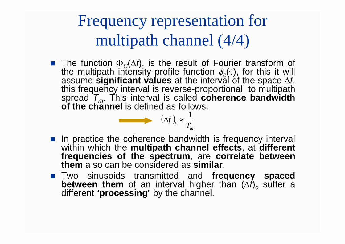
The function C(f), is the result of Fourier transform ofthe multipath intensity profile function fc(t), for this it willassume significant values at the interval of the space f,this frequency interval is reverse-proportional to multipathspread Tm. This interval is called coherence bandwidthof the channel is defined as follows:
In practice the coherence bandwidth is frequency intervalwithin which the multipath channel effects, at differentfrequencies of the spectrum, are correlate betweenthem a so can be considered as similar.
Two sinusoids transmitted and frequency spacedbetween them of an interval higher than (f)c suffer adifferent “processing” by the channel.
m
c Tf 1
Frequency selectivity of multipath channel
If coherence bandwidth (f )c is narrower thanbandwidth of the signal transmitted, the channel iscalled frequency selective (frequency selectivefading). In this case the signal transmitted issubjected to different and multiple distortionscased by multipath fading.
If coherence bandwidth is larger than bandwidth ofthe signal transmitted, the channel is called notfrequency selective (frequency non-selective fadingor flat fading). In this case the signal transmitted issubjected to uniform distortion in its bandwidth
Temporal representation of multipath channel (1/3)
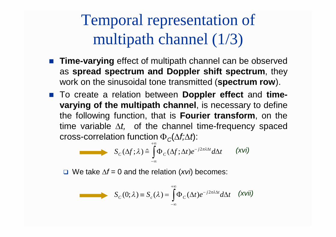
Time-varying effect of multipath channel can be observedas spread spectrum and Doppler shift spectrum, theywork on the sinusoidal tone transmitted (spectrum row).
To create a relation between Doppler effect and time-varying of the multipath channel, is necessary to definethe following function, that is Fourier transform, on thetime variable t, of the channel time-frequency spacedcross-correlation function C(f;t):
We take f = 0 and the relation (xvi) becomes:
tdetffS tjCC
2);(ˆ);( (xvi)
tdetSS tjCcC
2)()();0( (xvii)
Temporal representation of multipath channel (2/3)
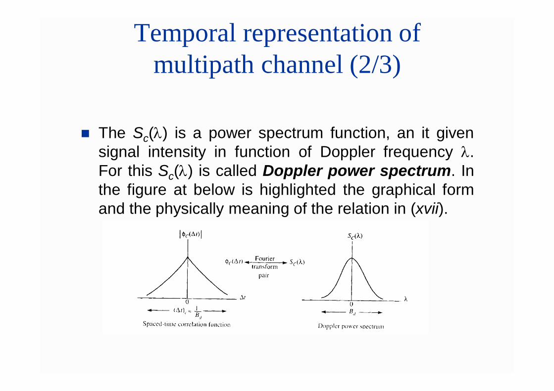
The Sc(l) is a power spectrum function, an it givensignal intensity in function of Doppler frequency l.For this Sc(l) is called Doppler power spectrum. Inthe figure at below is highlighted the graphical formand the physically meaning of the relation in (xvii).
Temporal representation of multipath channel (3/3)
From the relation (xvi) is shown that, if the channel is time-invariant, C(t)=1 and the function Sc(l) becomes aDirac delta. In this case there aren’t time variations inthe channel and there aren’t spread spectrum in thetransmission of one sinusoidal tone.
The range of l for which Sc(l) has non zero values iscalled channel Doppler-spread Bd .
Sc(l) is put in relation with, C(t) from Fourier transform,the inverse of Bd is a measure of channel coherencetime, that is time interval of observation during whichchannel effects on signal transmitted are correlatedbetween them and can be considered as similar.
d
c Bt 1
Multipath channel is characterize by slowlytime variations and it has high coherencetime which corresponds to low Dopplerspread (slow fading channel).
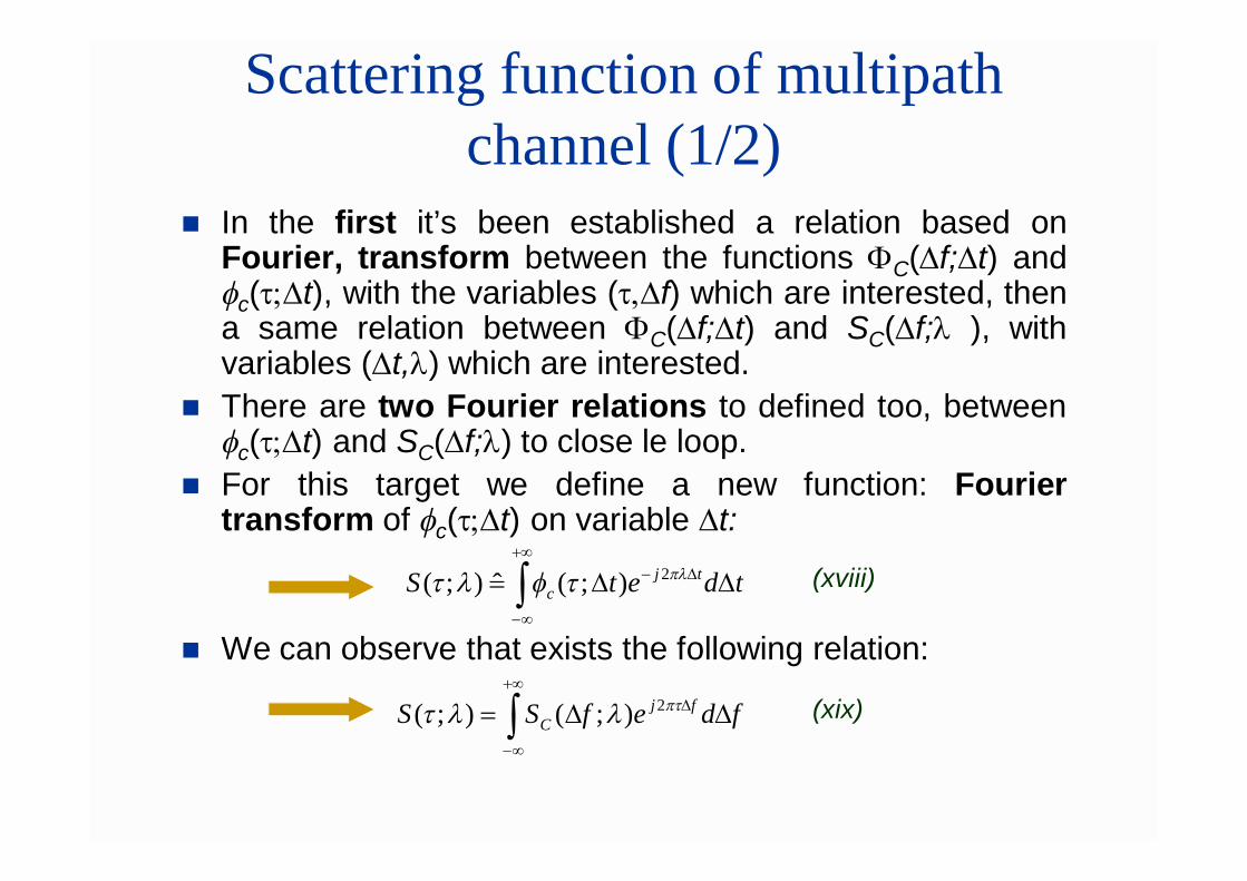
Scattering function of multipath channel (1/2)
In the first it’s been established a relation based onFourier, transform between the functions C(f;t) andfc(t;t), with the variables (t,f) which are interested, thena same relation between C(f;t) and SC(f;l ), withvariables (t,l) which are interested.
There are two Fourier relations to defined too, betweenfc(t;t) and SC(f;l) to close le loop.
For this target we define a new function: Fouriertransform of fc(t;t) on variable t:
We can observe that exists the following relation:
tdetS tjc
f 2);(ˆ);( (xviii)
fdefSS fjC
2);();( (xix)
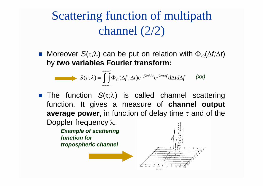
Scattering function of multipath channel (2/2)
Moreover S(t;l) can be put on relation with C(f;t)by two variables Fourier transform:
The function S(t;l) is called channel scatteringfunction. It gives a measure of channel outputaverage power, in function of delay time t and of theDoppler frequency l.
Example of scattering function for tropospheric channel
ftddeetfS fjtjC
22);();( (xx)
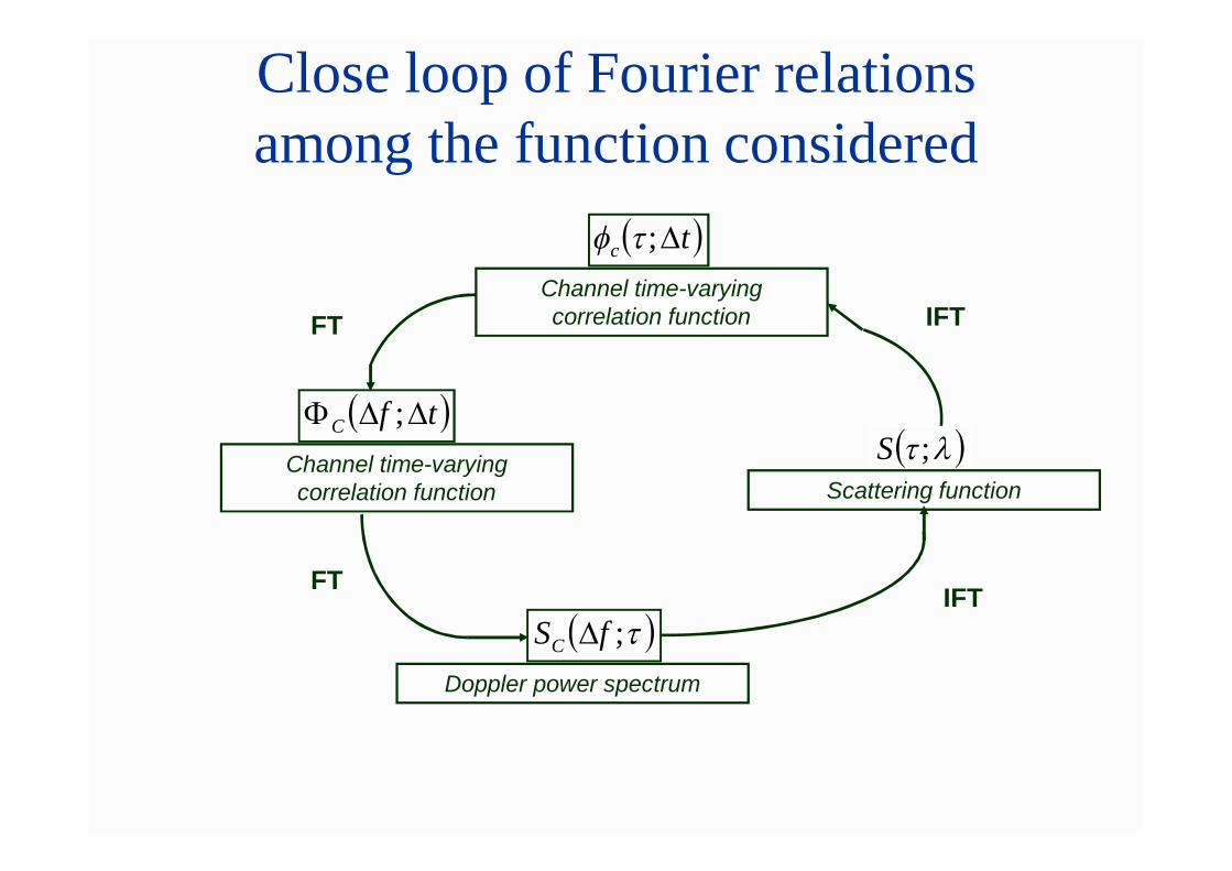
Close loop of Fourier relations among the function considered
tc ;fChannel time-varying correlation function
tfC ;
FT
Channel time-varying correlation function
FT
;fSC Doppler power spectrum
;SScattering function
IFT
IFT
Effects of signal characteristics on the choice of the multipath channel model (1/4)
After the analysis of statistical characterizations of time-varying multipath transmission channels, now we considermost important aspect for a telecommunication systems:the effects about the characteristics of the signaltransmitted for the choice of the channel model moreappropriate for the signal.
sl(t) is equivalent low pass of the signal transmitted onthe channel and Sl(f) is its spectrum. The equivalent lowpass of the signal received can be indicated as follows: In terms of functions time domain mapping:
In terms of function frequency domain mapping:
dtstctr ll )(;)(
dfefStfCtr ftjll
2)(;)(
(xxi)
(xxii)
Effects of signal characteristics on the choice of the multipath channel model (2/4)
We suppose to transmit the basic impulse with a rate equal torate 1/T, where T is signalling interval, amplitude or phasemodulated, or both. Signal bandwidth W is proportional to 1/T.
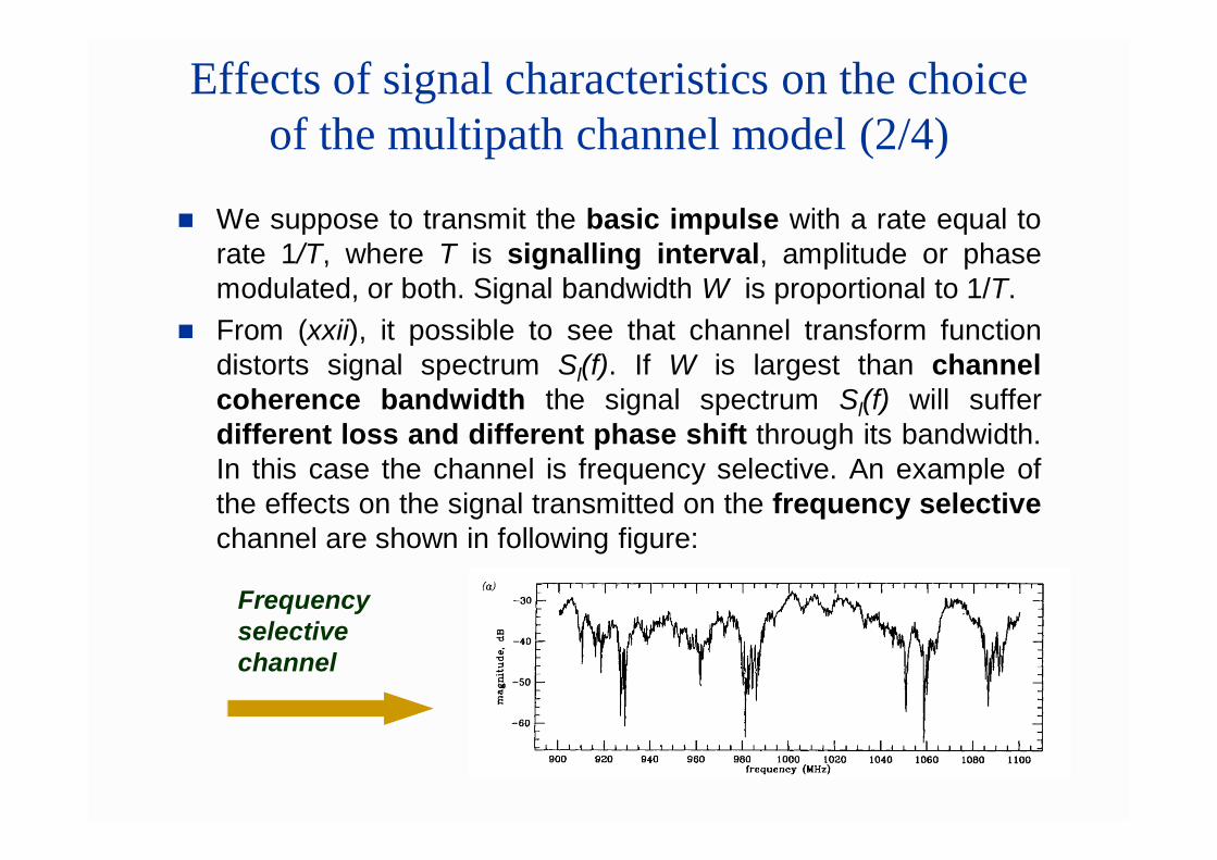
From (xxii), it possible to see that channel transform functiondistorts signal spectrum Sl(f). If W is largest than channelcoherence bandwidth the signal spectrum Sl(f) will sufferdifferent loss and different phase shift through its bandwidth.In this case the channel is frequency selective. An example ofthe effects on the signal transmitted on the frequency selectivechannel are shown in following figure:
Frequency selective channel
Effects of signal characteristics on the choice of the multipath channel model (3/4)
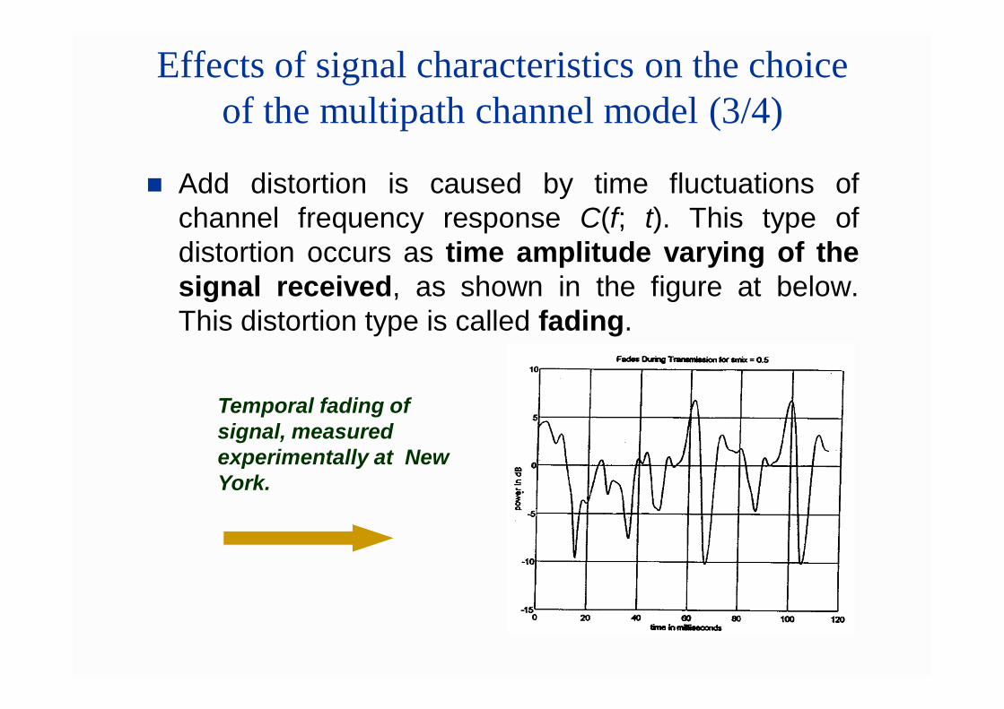
Add distortion is caused by time fluctuations ofchannel frequency response C(f; t). This type ofdistortion occurs as time amplitude varying of thesignal received, as shown in the figure at below.This distortion type is called fading.
Temporal fading of signal, measured experimentally at New York.
Effects of signal characteristics on the choice of the multipath channel model (4/4)
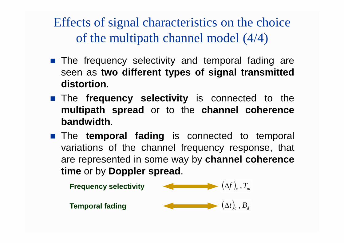
The frequency selectivity and temporal fading areseen as two different types of signal transmitteddistortion.
The frequency selectivity is connected to themultipath spread or to the channel coherencebandwidth.
The temporal fading is connected to temporalvariations of the channel frequency response, thatare represented in some way by channel coherencetime or by Doppler spread.
Frequency selectivity mc Tf ,
Temporal fading dc Bt ,
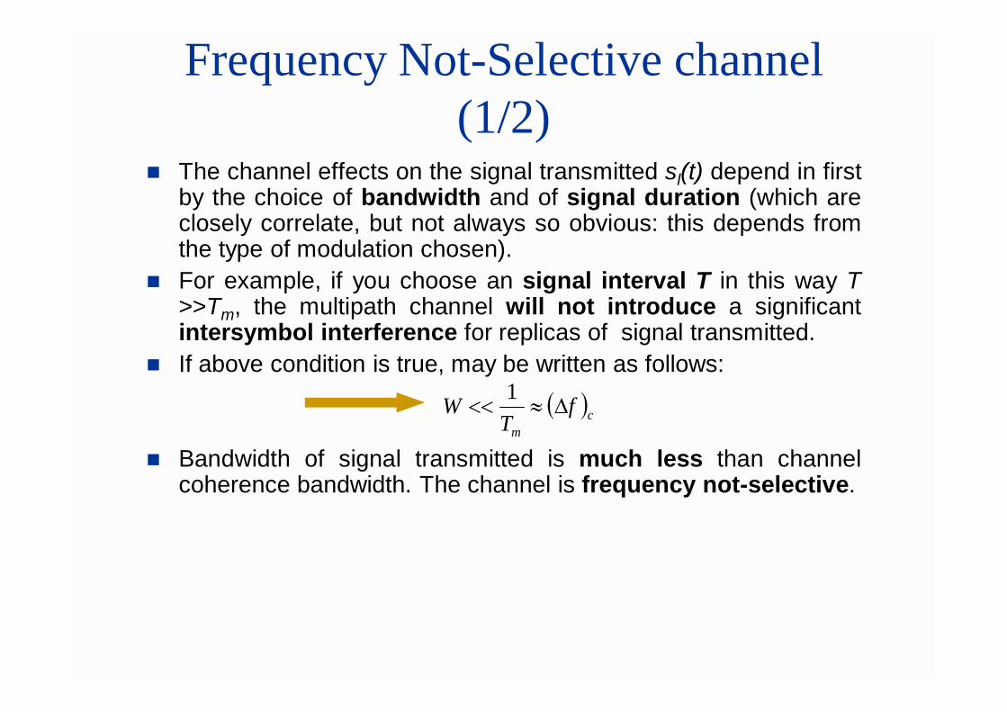
Frequency Not-Selective channel (1/2)
The channel effects on the signal transmitted sl(t) depend in firstby the choice of bandwidth and of signal duration (which areclosely correlate, but not always so obvious: this depends fromthe type of modulation chosen).
For example, if you choose an signal interval T in this way T>>Tm, the multipath channel will not introduce a significantintersymbol interference for replicas of signal transmitted.
If above condition is true, may be written as follows:
Bandwidth of signal transmitted is much less than channelcoherence bandwidth. The channel is frequency not-selective.
cm
fT
W 1
Frequency Not-Selective channel (2/2)
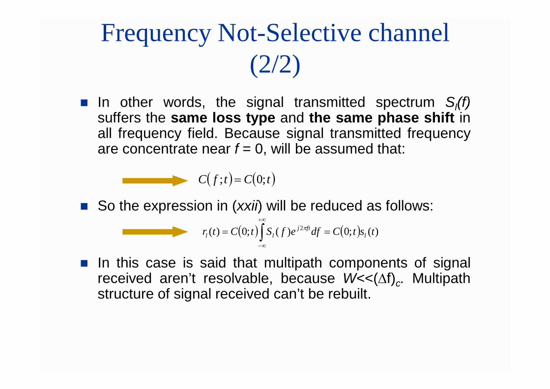
In other words, the signal transmitted spectrum Sl(f)suffers the same loss type and the same phase shift inall frequency field. Because signal transmitted frequencyare concentrate near f = 0, will be assumed that:
So the expression in (xxii) will be reduced as follows:
In this case is said that multipath components of signalreceived aren’t resolvable, because W<<(f)c. Multipathstructure of signal received can’t be rebuilt.
tCtfC ;0;
)(;0)(;0)( 2 tstCdfefStCtr lftj
ll
Channel characterized by slow fading (1/3)
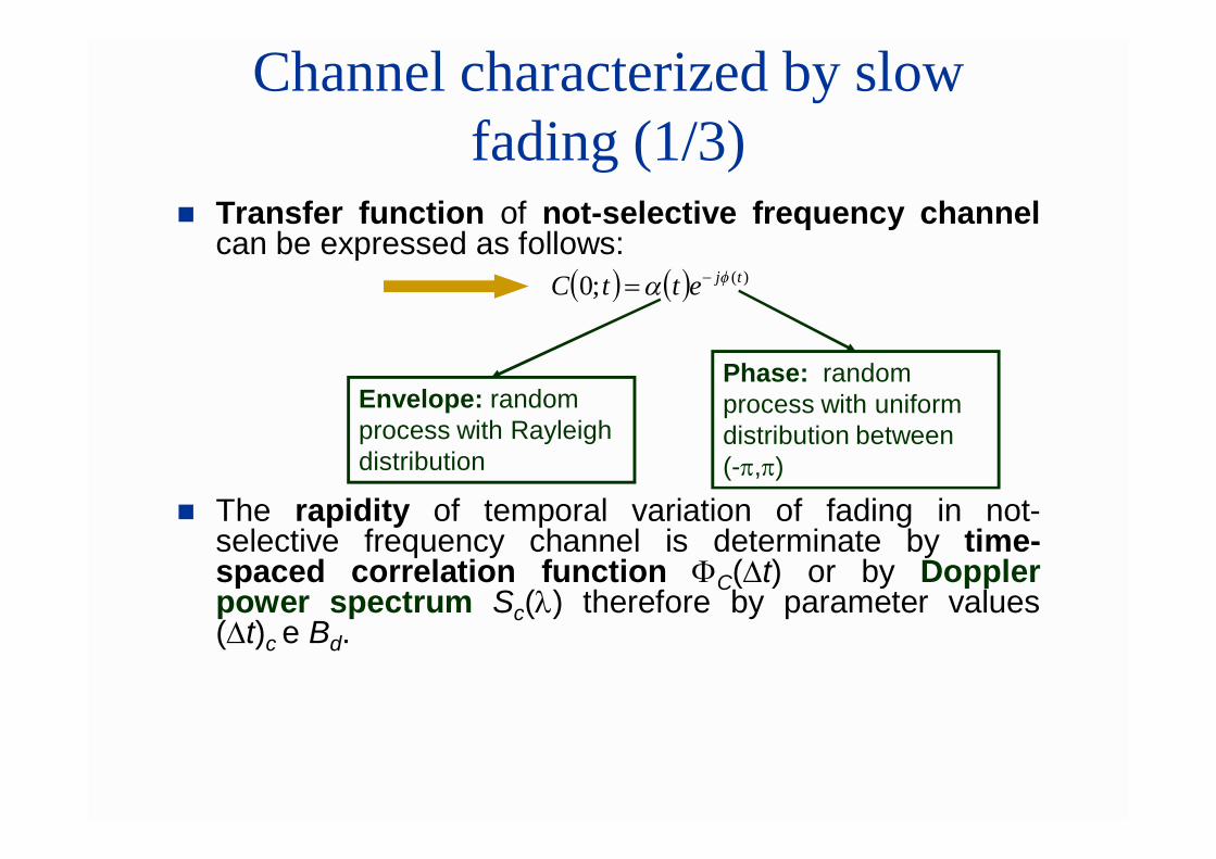
Transfer function of not-selective frequency channelcan be expressed as follows:
The rapidity of temporal variation of fading in not-selective frequency channel is determinate by time-spaced correlation function C(t) or by Dopplerpower spectrum Sc(l) therefore by parameter values(t)c e Bd.
)(;0 tjettC f
Envelope: random process with Rayleigh distribution
Phase: random process with uniform distribution between (-p,p)
Channel characterized by slow fading (2/3)
It is supposed can be selected a value of W so thatW<<(f)c and at the same time a signal interval value Tsuch that T<<(t)c.
As T is less than time of coherence channel. The channelloss and phase shift will be practically fixed for allduration of the symbol transmitted. When this condition isverified we can say that the channel is characterized byslow fading (slowly fading channel).
Moreover when W = 1/T, the condition that the channel isnot-selective and slowly fading channel at the same time,for this the product of TmBd is less than 1.
The product of TmBd is called spread factor. If TmBd<1,the channel I called underspread, otherwise the channelis called overspread.
Channel characterized by slow fading (3/3)
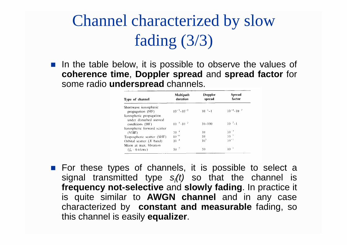
In the table below, it is possible to observe the values ofcoherence time, Doppler spread and spread factor forsome radio underspread channels.
For these types of channels, it is possible to select asignal transmitted type sl(t) so that the channel isfrequency not-selective and slowly fading. In practice itis quite similar to AWGN channel and in any casecharacterized by constant and measurable fading, sothis channel is easily equalizer.
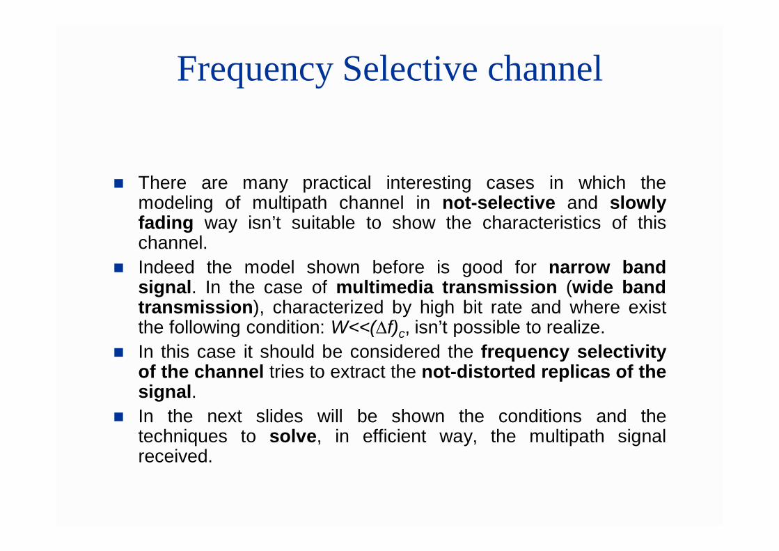
Frequency Selective channel
There are many practical interesting cases in which themodeling of multipath channel in not-selective and slowlyfading way isn’t suitable to show the characteristics of thischannel.
Indeed the model shown before is good for narrow bandsignal. In the case of multimedia transmission (wide bandtransmission), characterized by high bit rate and where existthe following condition: W<<(f)c, isn’t possible to realize.
In this case it should be considered the frequency selectivityof the channel tries to extract the not-distorted replicas of thesignal.
In the next slides will be shown the conditions and thetechniques to solve, in efficient way, the multipath signalreceived.
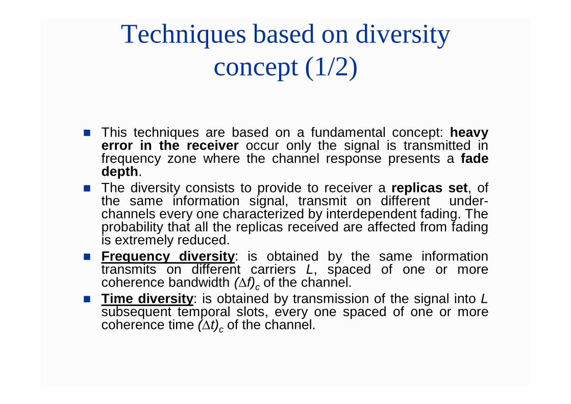
Techniques based on diversity concept (1/2)
This techniques are based on a fundamental concept: heavyerror in the receiver occur only the signal is transmitted infrequency zone where the channel response presents a fadedepth.
The diversity consists to provide to receiver a replicas set, ofthe same information signal, transmit on different under-channels every one characterized by interdependent fading. Theprobability that all the replicas received are affected from fadingis extremely reduced.
Frequency diversity: is obtained by the same informationtransmits on different carriers L, spaced of one or morecoherence bandwidth (f)c of the channel.
Time diversity: is obtained by transmission of the signal into Lsubsequent temporal slots, every one spaced of one or morecoherence time (t)c of the channel.
Techniques based on diversity concept (2/2)
Multiple antennas used: the first two methods aren’tvery effective, because they are translated in gratewaste of the bandwidth, the technique is more usedin real case: is used in antennas set to receive,separated between them by an appropriate distance,are able to intercept different signal propagationpaths.
Generally it is possible to space one antenna fromthe other at least by 10 wavelenght, to consentthem to receive different independent paths.
The use of the multiple antennas is quite expensive,for the purchase and installation of the antennas set.
Other techniques based on diversity concept
Frequency-hopping (FH): the signal transmitted hops fromfrequency to the other, second a predefined temporal sequence,into of a given bandwidth. At the receiver will be necessary torebuild the hop sequence to demodulate the signal. This concept isused in Spread Spectrum techniques based on FrequencyHopping (FH/SS). The target is minimize the number of the hopare distorted by the selective sequence channel.
Signal transmission on multiple carriers spaced between themin orthogonal way: this concept is used in OFDM e DTM (wheredifferent symbols are transmitted on different carriers) and MC-CDMA (the same symbol is transmitted on different carriers).The orthogonal spacing between different carriers (equal to k/T, k= 0,1,..,N), allows high efficient to information recovery, robustnessthan multipath fading easy implementation (“full digital” witharchitecture based on FFT realized by DSP technology).
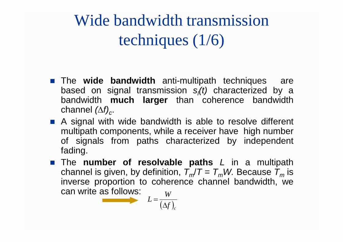
Wide bandwidth transmission techniques (1/6)
The wide bandwidth anti-multipath techniques arebased on signal transmission sl(t) characterized by abandwidth much larger than coherence bandwidthchannel (f)c.
A signal with wide bandwidth is able to resolve differentmultipath components, while a receiver have high numberof signals from paths characterized by independentfading.
The number of resolvable paths L in a multipathchannel is given, by definition, Tm/T = TmW. Because Tm isinverse proportion to coherence channel bandwidth, wecan write as follows:
cfWL
Wide bandwidth transmission techniques (2/6)
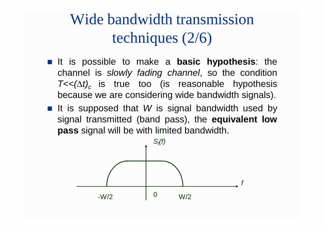
It is possible to make a basic hypothesis: thechannel is slowly fading channel, so the conditionT<<(t)c is true too (is reasonable hypothesisbecause we are considering wide bandwidth signals).
It is supposed that W is signal bandwidth used bysignal transmitted (band pass), the equivalent lowpass signal will be with limited bandwidth.
0 W/2-W/2
Sl(f)
f
Wide bandwidth transmission techniques (3/6)
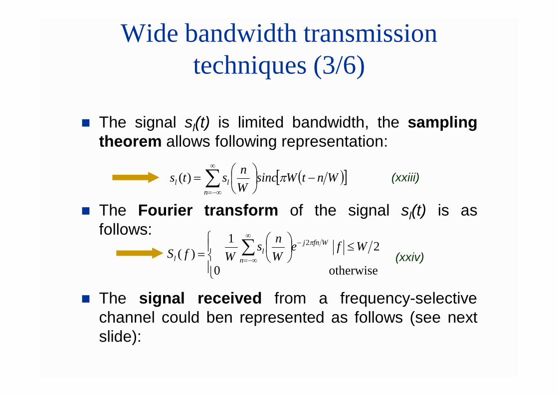
The signal sl(t) is limited bandwidth, the samplingtheorem allows following representation:
The Fourier transform of the signal sl(t) is asfollows:
The signal received from a frequency-selectivechannel could ben represented as follows (see nextslide):
WntWsincWnsts
nll
)(
otherwise 0
2 1)(
2
Wfe
Wns
WfSWfnj
nl
l
(xxiii)
(xxiv)
Wide bandwidth transmission techniques (4/6)
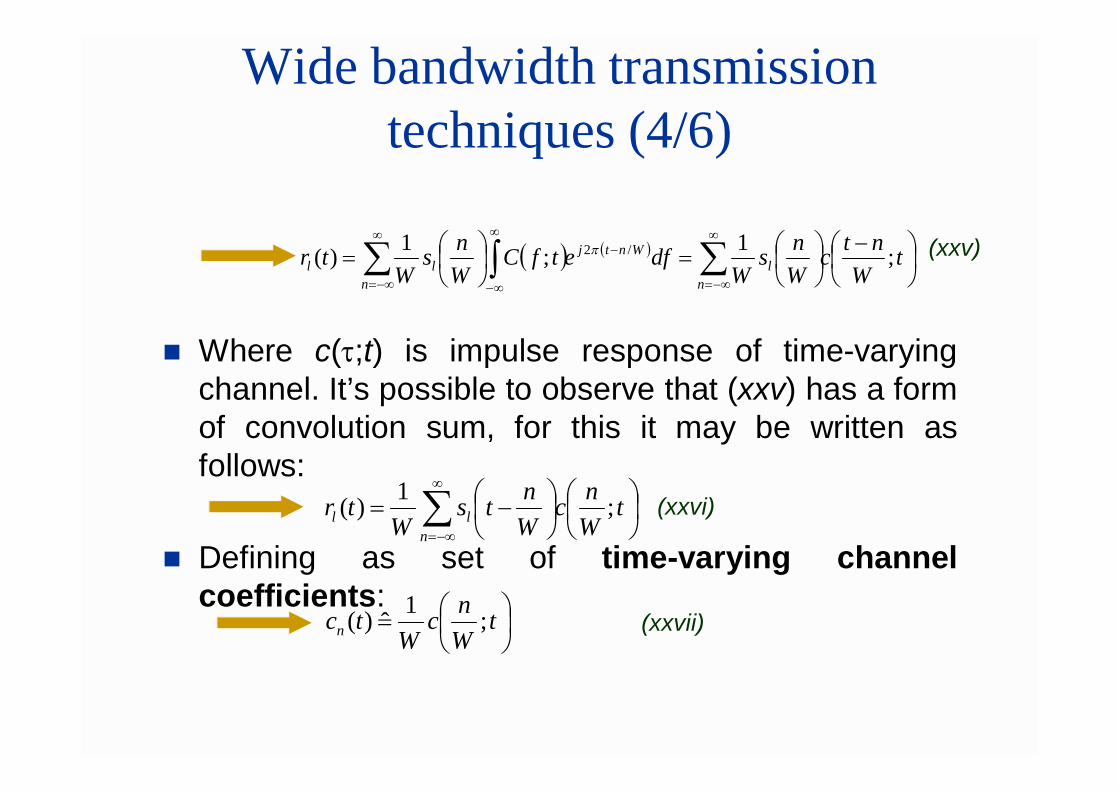
Where c(t;t) is impulse response of time-varyingchannel. It’s possible to observe that (xxv) has a formof convolution sum, for this it may be written asfollows:
Defining as set of time-varying channelcoefficients:
tW
ntcWns
WdfetfC
Wns
Wtr
nl
Wntj
nll ;1 ;1)( /2 (xxv)
nll t
Wnc
Wnts
Wtr ;1)( (xxvi)
tWnc
Wtcn ;1
ˆ)( (xxvii)
Wide bandwidth transmission techniques (5/6)
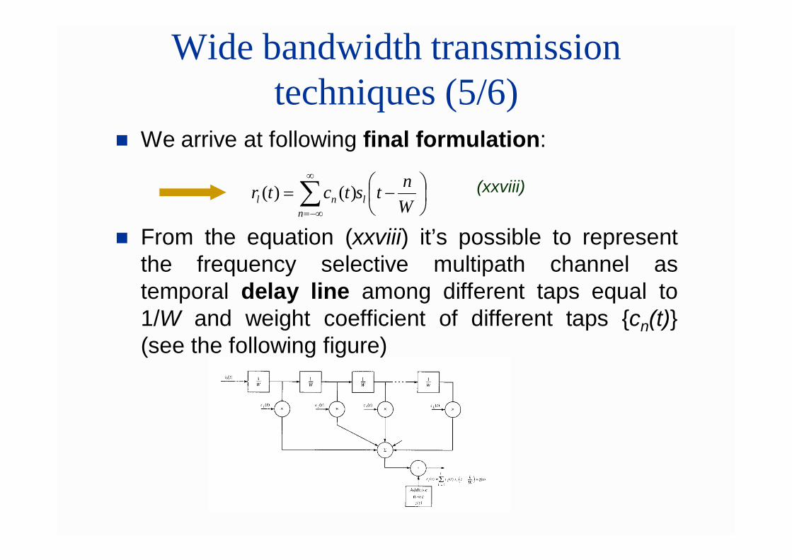
We arrive at following final formulation:
From the equation (xxviii) it’s possible to representthe frequency selective multipath channel astemporal delay line among different taps equal to1/W and weight coefficient of different taps {cn(t)}(see the following figure)
Wntstctr l
nnl )()( (xxviii)
Wide bandwidth transmission techniques (6/6)
So transmitting the signal, its equivalent low pass has bandwidth equal toW, where W >> (f)c we can obtain a profile resolution of the multipathfor the signal received with granularity equal to 1/W.
The delay line will be truncated to L = [TmW]+1 tap. The signal received(except channel noise) has the following equation:
Time-varying channel coefficients {cn(t)} are random process with complexvalues, stationary. Assuming as true, the uncorrelate scattering, like saidbefore, the {cn(t)} coefficients are mutually uncorrelated. In the case ofRayleight fading, the magnitude of {cn(t)} is distributed as Rayleight,while the phase is uniformly distributed between (-p,p).
Wntstctr l
L
nnl
1
)()( (xxix)
Narrow band signal format for transmission on selective frequency channels
A typical wide bandwidth signal used to realize the conditionalW>>(f)c is Direct Sequences Spread Spectrum (DS/SS).
This signal is obtained multiplying the information bit flow withbinary pseudo-random signal, characterized by signal rate muchhigh than original information signal.
To transmit the information on very large bandwidth by DS/SStechniques, in way to oppose the degradations introduce bymultipath fading, is a typical approach common used by manystandard for wireless digital communications: IEEE 802.11 for data transmission on WLAN local network;
IS-95 USA standard for mobile phone;
UMTS future European standard for radio-mobile communication;
Satellite System low orbit GLOBALSTAR for mobile phone.
Optimum receiver for selective frequency channels (1/4)
Let us consider the optimal receiving of digital signal on selectivefrequency channel, modeled as delay line with time-varyingweights and statistically independent, similar at the channel shownbefore.
The signal received is composed by L replicas of original signaltransmitted. More large is transmission bandwidth W and morehigh will be the probability to find a not-distorted replica, so it canbe usable to extract the information transmitted.
Let us consider a binary signal on the channel (for example BPSKmodulation). Will be obtained two base-signals sl1(t) and sl2(t) whichcan be antipodal or orthogonal. Their duration is chosen as T>>Tm,in this way it’s possible to neglect any intersymbol interferencetypes for multipath fading.
In following treatment will be considered the transmission of DS/SSsignal with BPSK modulation, this is a classic case study of thewide bandwidth receiving on selective frequency channels.
Optimum receiver for selective frequency channels (2/4)
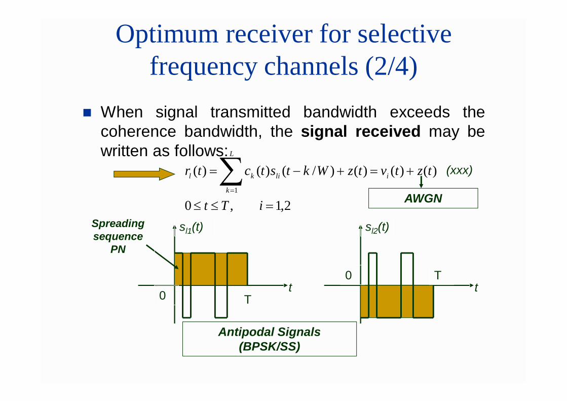
When signal transmitted bandwidth exceeds thecoherence bandwidth, the signal received may bewritten as follows:
2,1 ,0
)()()()/()()(1
iTt
tztvtzWktstctrL
k
ilikl (xxx)
sl1(t)
t0 T
sl2(t)
t0 T
Antipodal Signals (BPSK/SS)
AWGN
Spreading sequence
PN
Optimum receiver for selective frequency channels (3/4)
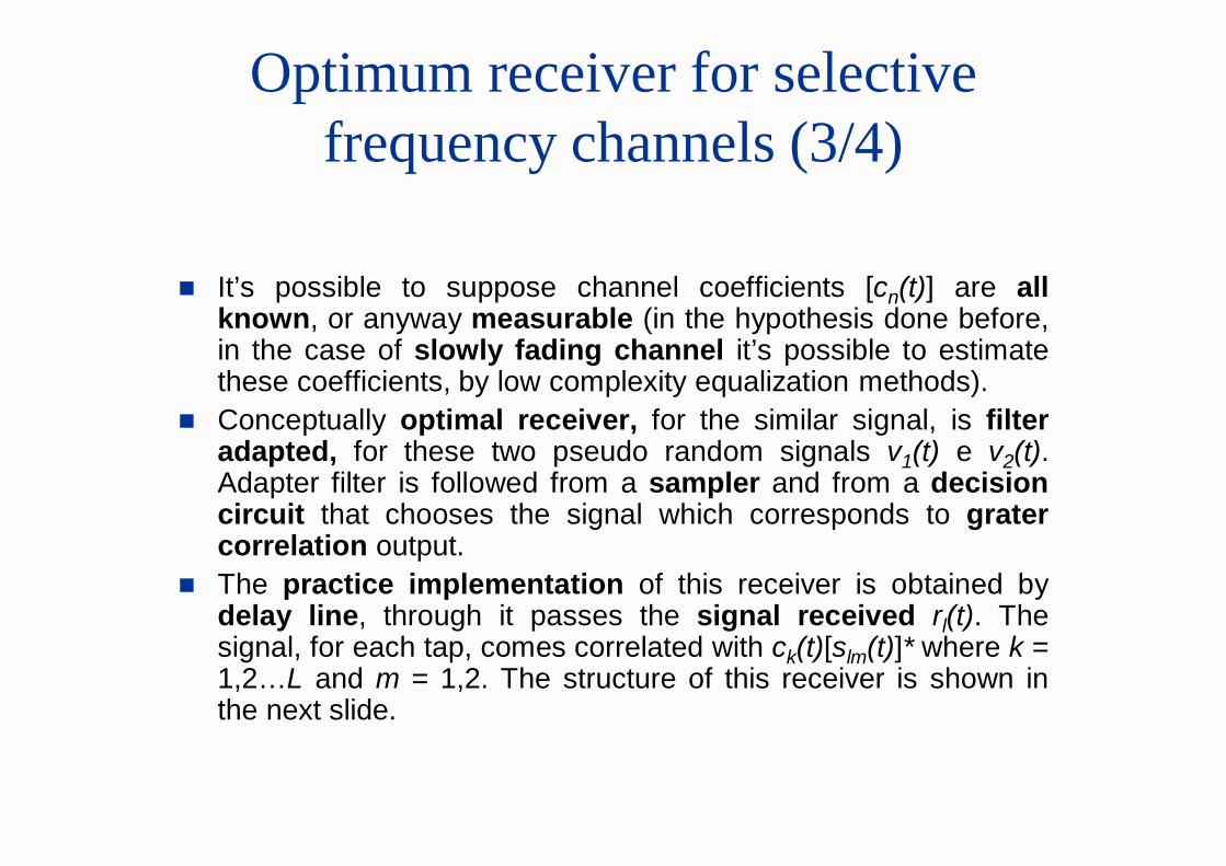
It’s possible to suppose channel coefficients [cn(t)] are allknown, or anyway measurable (in the hypothesis done before,in the case of slowly fading channel it’s possible to estimatethese coefficients, by low complexity equalization methods).
Conceptually optimal receiver, for the similar signal, is filteradapted, for these two pseudo random signals v1(t) e v2(t).Adapter filter is followed from a sampler and from a decisioncircuit that chooses the signal which corresponds to gratercorrelation output.
The practice implementation of this receiver is obtained bydelay line, through it passes the signal received rl(t). Thesignal, for each tap, comes correlated with ck(t)[slm(t)]* where k =1,2…L and m = 1,2. The structure of this receiver is shown inthe next slide.
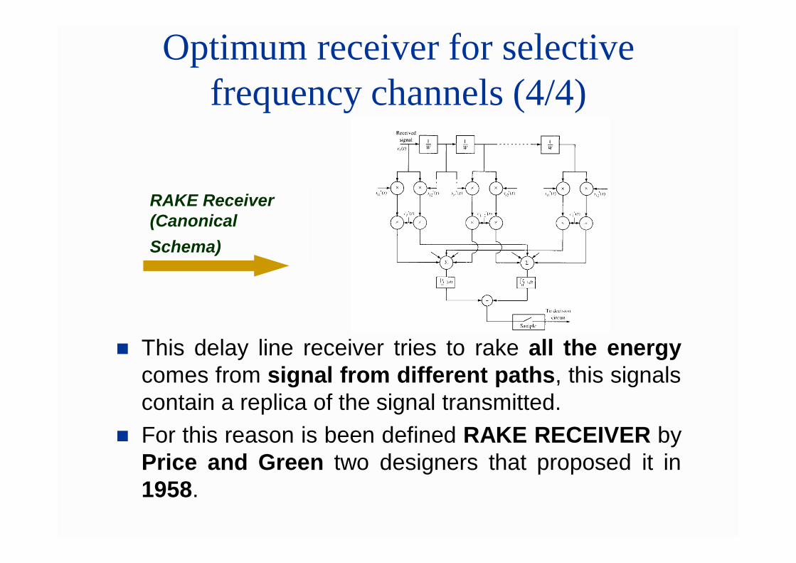
Optimum receiver for selective frequency channels (4/4)
This delay line receiver tries to rake all the energycomes from signal from different paths, this signalscontain a replica of the signal transmitted.
For this reason is been defined RAKE RECEIVER byPrice and Green two designers that proposed it in1958.
RAKE Receiver (Canonical Schema)
Notes on RAKE receiver performances (1/2)
The capacity of RAKE to extract the replicas from signal, tocompensate fading effects, depends in first from W transmissionbandwidth dimension. A RAKE receiver doesn’t work wellwhen the transmission bandwidth W is comparable withchannel coherence bandwidth.
Canonical RAKE receiver performances are conditional toreliability of channel coefficient estimate. Reliable estimate ofthese coefficients is possible to realize by low complexityalgorithm if the fading is slow enough, for example if (t)c>100T,where T is signal interval.
When channel coefficients aren’t estimated accurately, or is toocostly because the fading is too fast (for example in urban radiomobile channel), it’s possible to use alternative RAKE structure.In this devise integrator outputs aren’t combined as weightedsum but is used a square combination (as shown in the nextslide).
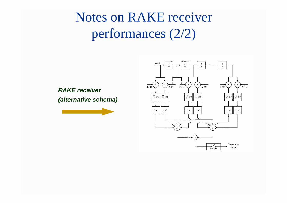
Notes on RAKE receiver performances (2/2)
RAKE receiver (alternative schema)


![HERTZIAN LINKS - unige.it · 2020. 4. 26. · References [1] Theodore S. Rappaport, Wireless Communications, 2ed, Prentice Hall, 2002 [2] J.G. Proakis, Communication Systems (Fifth](https://img.pdfslide.us/doc/110x75/60ba0d10c3caf26f4213bca6/hertzian-links-unigeit-2020-4-26-references-1-theodore-s-rappaport-wireless.jpg)

![c Copyright 2012 Civil-Comp Press Notice Changes ...eprints.qut.edu.au/61673/1/Suitability_of_using_PEEQ_to...Vehicle Dynamics [3] explains the procedure of calculating Hertzian parameters](https://img.pdfslide.us/doc/110x75/5b0470e67f8b9a41528c7fb3/c-copyright-2012-civil-comp-press-notice-changes-dynamics-3-explains-the-procedure.jpg)