Radiation View factors - ¡Bienvenidos! — Portal …webserver.dmt.upm.es/~isidoro/tc3/Radiation View factors... · Web viewView factor definition2 View factor algebra3 View factors

111EquationChapter 1Section 1 RADIATIVE VIEW FACTORS

View factor definition....................................................................................................................................2View factor algebra....................................................................................................................................3View factors with two-dimensional objects...............................................................................................4

Very-long triangular enclosure..............................................................................................................5The crossed string method.....................................................................................................................7

View factor with an infinitesimal surface: the unit-sphere and the hemicube methods............................8With spheres..................................................................................................................................................9

Patch to a sphere........................................................................................................................................9Frontal....................................................................................................................................................9Level......................................................................................................................................................9Tilted......................................................................................................................................................9

Patch to a spherical cap............................................................................................................................10Sphere to concentric external cylinder.....................................................................................................11Disc to frontal sphere...............................................................................................................................11Cylinder to large sphere...........................................................................................................................12Cylinder to its hemispherical closing cap................................................................................................12Sphere to sphere.......................................................................................................................................13

Small to very large...............................................................................................................................13Concentric spheres...............................................................................................................................13Sphere to concentric hemisphere.........................................................................................................13

Hemispheres.............................................................................................................................................13Concentric hemispheres.......................................................................................................................13Small hemisphere frontal to large sphere............................................................................................14Hemisphere to planar surfaces.............................................................................................................14

Spherical cap to base disc........................................................................................................................15With cylinders..............................................................................................................................................16

Cylinder to large sphere...........................................................................................................................16Cylinder to its hemispherical closing cap................................................................................................16Very-long cylinders.................................................................................................................................16

Concentric cylinders............................................................................................................................16Concentric cylinder to hemi-cylinder..................................................................................................16Concentric frontal hemi-cylinders.......................................................................................................16Concentric opposing hemi-cylinders...................................................................................................17Hemi-cylinder to central strip..............................................................................................................17Hemi-cylinder to infinite plane............................................................................................................17Equal external cylinders.......................................................................................................................18

Radiative view factors 1

Equal external hemi-cylinders.............................................................................................................18Planar strip to cylinder.........................................................................................................................18Wire to parallel cylinder......................................................................................................................19

Finite cylinders........................................................................................................................................20Base to lateral surface..........................................................................................................................20Disc to coaxial cylinder.......................................................................................................................20Equal finite concentric cylinders.........................................................................................................20Outer surface of cylinder to annular disc joining the base..................................................................21Cylindrical rod to coaxial disc at one end............................................................................................21

With plates and discs...................................................................................................................................22Parallel configurations.............................................................................................................................22

Patch to disc.........................................................................................................................................22Patch to annulus...................................................................................................................................22Patch to rectangular plate.....................................................................................................................22Equal square plates..............................................................................................................................22Equal rectangular plates.......................................................................................................................23Rectangle to rectangle..........................................................................................................................23Unequal coaxial square plates..............................................................................................................23Box inside concentric box....................................................................................................................24Equal discs...........................................................................................................................................25Unequal discs.......................................................................................................................................25Strip to strip.........................................................................................................................................25Patch to infinite plate...........................................................................................................................26

Perpendicular configurations...................................................................................................................26Patch to rectangular plate.....................................................................................................................26Square plate to rectangular plate..........................................................................................................26Rectangular plate to equal rectangular plate........................................................................................27Rectangular plate to unequal rectangular plate....................................................................................27Rectangle to rectangle..........................................................................................................................28Strip to strip.........................................................................................................................................28Cylindrical rod to coaxial disc at tone end..........................................................................................28

Tilted strip configurations........................................................................................................................28Equal adjacent strips............................................................................................................................28Triangular prism..................................................................................................................................28

Numerical computation................................................................................................................................29References....................................................................................................................................................30

VIEW FACTOR DEFINITION

The view factor F12 is the fraction of energy exiting an isothermal, opaque, and diffuse surface 1 (by emission or reflection), that directly impinges on surface 2 (to be absorbed, reflected, or transmitted). View factors depend only on geometry. Some view factors having an analytical expression are compiled below. We will use the subindices in F12 without a separator when only a few single view-factors are concerned, although more explicit versions, like F1,2 , or even better, F1→2, could be used.


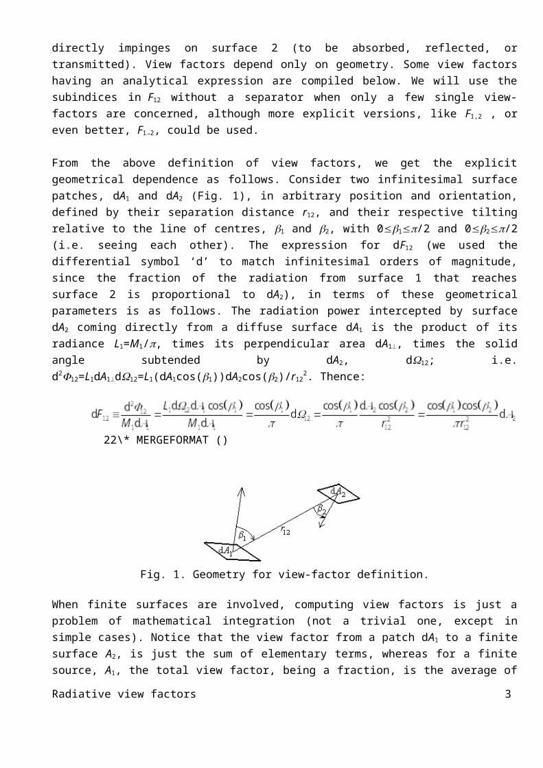
From the above definition of view factors, we get the explicit geometrical dependence as follows. Consider two infinitesimal surface patches, dA1 and dA2 (Fig. 1), in arbitrary position and orientation, defined by their separation distance r12, and their respective tilting relative to the line of centres, 1 and 2, with 01/2 and 02/2 (i.e. seeing each other). The expression for dF12 (we used the differential symbol ‘d’ to match infinitesimal orders of magnitude, since the fraction of the radiation from surface 1 that reaches surface 2 is proportional to dA2), in terms of these geometrical parameters is as follows. The radiation power intercepted by surface dA2 coming directly from a diffuse surface dA1 is the product of its radiance L1=M1/, times its perpendicular area dA1, times the solid angle subtended by dA2, d12; i.e. d212=L1dA1d12=L1(dA1cos(1))dA2cos(2)/r12

2. Thence:

22\*MERGEFORMAT ()

Fig. 1. Geometry for view-factor definition.

When finite surfaces are involved, computing view factors is just a problem of mathematical integration (not a trivial one, except in simple cases). Notice that the view factor from a patch dA1 to a finite surface A2, is just the sum of elementary terms, whereas for a finite source, A1, the total view factor, being a fraction, is the average of the elementary terms, i.e. the view factor between finite surfaces A1 and A2 is:

33\* MERGEFORMAT ()

Recall that the emitting surface (exiting, in general) must be isothermal, opaque, and Lambertian (a perfect diffuser for emission and reflection), and, to apply view-factor algebra, all surfaces must be isothermal, opaque, and Lambertian. Finally notice that F12 is proportional to A2 but not to A1.

View factor algebra

When considering all the surfaces under sight from a given one (let the enclosure have N different surfaces, all opaque, isothermal, and diffuse), several general relations can be established among the N2

possible view factors Fij, what is known as view factor algebra: Bounding. View factors are bounded to 0Fij≤1 by definition (the view factor Fij is the fraction

of energy exiting surface i, that impinges on surface j).Radiative view factors 3

Closeness. Summing up all view factors from a given surface in an enclosure, including the possible self-view factor for concave surfaces, , because the same amount of radiation emitted by a surface must be absorbed.

Reciprocity. Noticing from the above equation that dAidFij=dAjdFji=(cosicosj/(rij2))dAidAj, it

is deduced that . Distribution. When two target surfaces (j and k) are considered at once, , based

on area additivity in the definition. Composition. Based on reciprocity and distribution, when two source areas are considered

together, .

One should stress the importance of properly identifying the surfaces at work; e.g. the area of a square plate of 1 m in side may be 1 m2 or 2 m2, depending on our considering one face or the two faces. Notice that the view factor from a plate 1 to a plate 2 is the same if we are considering only the frontal face of 2 or its two faces, but the view factor from a plate 1 to a plate 2 halves if we are considering the two faces of 1, relative to only taking its frontal face.

For an enclosure formed by N surfaces, there are N2 view factors (each surface with all the others and itself). But only N(N1)/2 of them are independent, since another N(N1)/2 can be deduced from reciprocity relations, and N more by closeness relations. For instance, for a 3-surface enclosure, we can define 9 possible view factors, 3 of which must be found independently, another 3 can be obtained from

, and the remaining 3 by .

View factors with two-dimensional objects

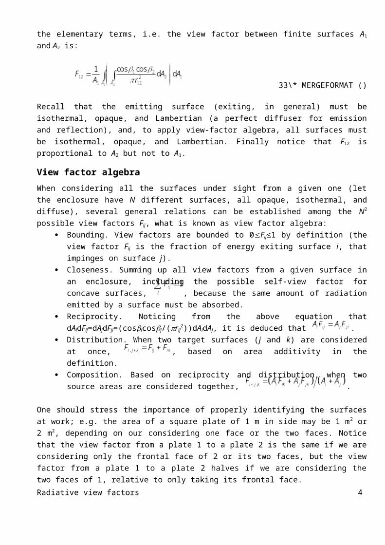
Consider two infinitesimal surface patches, dA1 and dA2, each one on an infinitesimal long parallel strip as shown in Fig. 2. The view factor dF12 is given by 2, where the distance between centres, r12, and the angles 1 and2 between the line of centres and the respective normal are depicted in the 3D view in Fig. 2a, but we want to put them in terms of the 2D parameters shown in Fig. 2b (the minimum distance a=

, and the1 and2 angles when z=0, 10 and20), and the depth z of the dA2 location. The relationship are: r12= = , cos1=cos10cos, with cos1=y/r12=(y/a)(a/r12), cos10=y/a, cos=a/r12, and cos2=cos20cos, therefore, between the two patches:

44\*MERGEFORMAT ()


Fig. 2. Geometry for view-factor between two patches in parallel strips: a 3D sketch, b) profile view.

Expression 4 can be reformulated in many different ways; e.g. by setting d2A2=dwdz, where the ‘d2’ notation is used to match differential orders and dw is the width of the strip, and using the relation ad10=cos20dw. However, what we want is to compute the view factor from the patch dA1 to the whole strip from z=∞ to z=∞, what is achieved by integration of 4 in z:

55\*MERGEFORMAT ()

For instance, approximating differentials by small finite quantities, the fraction of radiation exiting a patch of A1=1 cm2, that impinges on a parallel and frontal strip (10=20=0) of width w=1 cm separated a distance a=1 m apart is F12=w/(2a)=0.01/(2·1)=0.005, i.e. a 0.5 %. It is stressed again that the exponent in the differential operator ‘d’ is used for consistency in infinitesimal order.

Now we want to know the view factor dF12 from an infinite strip dA1 (of area per unit length dw1) to an infinite strip dA2 (of area per unit length dw2), with the geometry presented in Fig. 2. It is clear from the infinite extent of strip dA2 that any patch d2A1=dw1dz1 has the same view factor to the strip dA2, so that the average coincides with this constant value and, consequently, the view factor between the two strips is precisely given by 5; i.e. following the example presented above, the fraction of radiation exiting a long strip of w1=1 cm width, that impinges on a parallel and frontal strip (10=20=0) of width w2=1 cm separated a distance a=1 m apart is F12=w2/(2a)=0.01/(2·1)=0.005, i.e. a 0.5 %.

Notice the difference in view factors between the two strips and the two patches in the same position as in Fig. 2b: using dA1 and dA2 in both cases, the latter (3D case) is given by the general expression 2, which takes the form dF12=cos10cos20dA2/(a2), whereas in the two-strip case (2D), it is dF12=cos10cos20dA2/(2a), where A2 has now units of length (width of the strip).

Very-long triangular enclosureConsider a long duct with the triangular cross section shown in Fig. 3. We may compute the view factor F12 from face 1 to face 2 (inside the duct) by double integration of the view factor from a strip of width dw1 in L1 to strip dw2 in L2; e.g. using de strip-to-strip view factor 5, the strip to finite band view factor is Radiative view factors 5

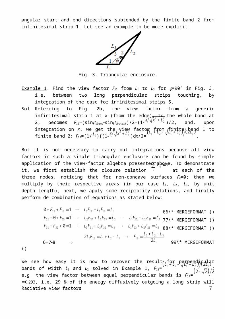
F12=cos10d10/2=(sin10endsin10start)/2, where 10start and 10end are the angular start and end directions subtended by the finite band 2 from infinitesimal strip 1. Let see an example to be more explicit.

Fig. 3. Triangular enclosure.

Example 1. Find the view factor F12 from L1 to L2 for =90º in Fig. 3, i.e. between two long perpendicular strips touching, by integration of the case for infinitesimal strips 5.

Sol. Referring to Fig. 2b, the view factor from a generic infinitesimal strip 1 at x (from the edge), to the whole band at 2, becomes F12=(sin10endsin10start)/2=(1 )/2, and, upon integration on x, we get the view factor from finite band 1 to finite band 2: F12=(1/ )(1 )dx/2=

.

But it is not necessary to carry out integrations because all view factors in such a simple triangular enclosure can be found by simple application of the view-factor algebra presented above. To demonstrate it, we first establish the closure relation at each of the three nodes, noticing that for non-concave surfaces Fii=0; then we multiply by their respective areas (in our case L1, L2, L3, by unit depth length); next, we apply some reciprocity relations, and finally perform de combination of equations as stated below:

66\* MERGEFORMAT ()

77\* MERGEFORMAT ()

88\* MERGEFORMAT ()

6+78 99\* MERGEFORMAT ()

We see how easy it is now to recover the result for perpendicular bands of width L1 and L2 solved in Example 1, F12= ; e.g. the view factor between equal perpendicular bands is F12= , i.e. 29 % of the energy diffusively outgoing a long strip will directly reach an equal strip perpendicular and hinged to the former, with the remaining 71 % being directed to the other side 3 (lost towards the environment if L3 is just an opening).

Even though we have implicitly assumed straight-line cross-sections (Fig. 3), the result 9 applies to convex triangles too (we only required Fii=0), using the real curvilinear lengths instead of the straight distances. As for concave bands, the best is to apply 9 to the imaginary straight-line triangle, and


afterwards solve for the trivial enclosure of the real concave shape and its corresponding virtual straight-line.

Example 2. Find the view factor F12 between two long hemicylindrical strips touching with perpendicular faces (Fig. E2).

Sol. Let 1’ and 2’ be the imaginary planar faces of the hemicyliners. From Example 1 applied to equal perpendicular straight strips, F1’2’= = =0.293, where L1’=L2’

are the diametrical strips to L1 and L2 (dashed in Fig. E2), which we can take as unit length; the enclose is completed with F1’3=1F1’2’=0,707. Let consider now the cylindrical surfaces; first, it is clear that the radiation arriving at 2’ (from 1’) will arrive at 2 also, i.e. F1’2’=F1’2; second, it is obvious that F1’1=1, i.e. all radiation outgoing downwards from the planar strip 1’ will go to 1, and, by the reciprocity relation, F11’=A1’F1’1/A1=1·F1’1/(/2)=2/= 0.637, and hence F11=1F11’’=12/=0,363. In summary, from the radiation cast by hemicylinder 1, a fraction F11=36 % goes against the same concave surface, and, from the remaining F11’=64 % that goes upwards, 29 % of it goes towards the right (surface 2), and the 71 % remaining impinged on surface 3; in consequence, F12=F11’F1’2=0.637·0.293= =0.186, F13=F11’F1’3= 0.637·0.707==0.450, and F11=12/=0.363 (check: 0.363+0.186+0.4501).

Fig. E2. Sketch to deduce the view factor F12 between two long hemicylinders (1) and (2).

Now we generalise this algebraic method of computing view factors in two-dimensional geometries to non-contact surfaces.

The crossed string methodFor any two non-touching infinitely-long bands, 1 and 2 (Fig. 4), one can also find all the view factors from simple algebraic relations as in the triangular enclosure before, extending the result 9 to what is known as crossed-string method:

1010\* MERGEFORMAT()


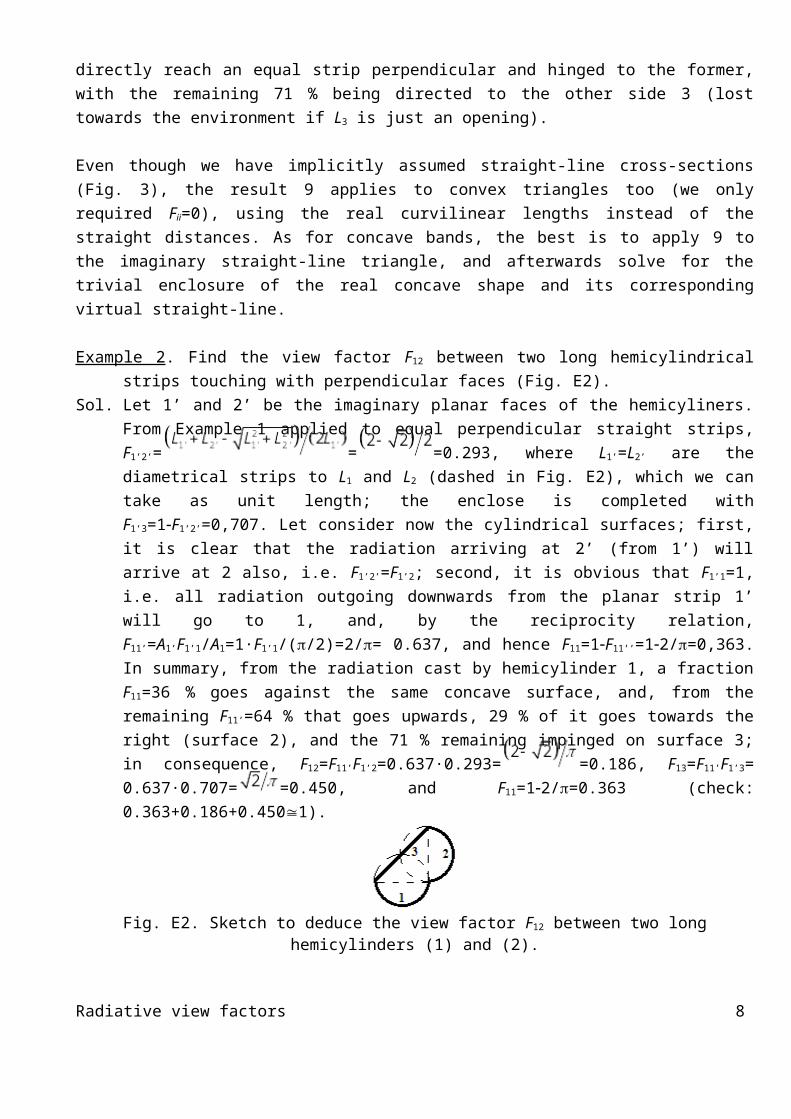
Fig. 4. Sketch used to deduce F12 in the general case of two infinitely long bands.

The result 10 is deduced by applying the triangular relation 9 to triangle 134 (shadowed in Fig. 4) and triangle 156, plus the closure relation to the quadrilateral 1326 (F13+F12+F16=1), namely:

1111\* MERGEFORMAT ()

This procedure to compute view factors in two-dimensional configurations (the crossed-string method), was first developed by H.C. Hottel in the 1950s. The extension to non-planar surfaces 1 and 2 is as already presented for triangular enclosures. A further extension is possible to cases where there are obstacles (two-dimensional, of course) partially protruding into sides 3 and/or 6 in the quadrilateral 1326 (Fig. 4); it suffices to account for the real curvilinear length of each string when stretched over the obstacles, as shown in the following example.

Example 3. Find the view factor between two long parallel cylinders of equal radii R, separated a distance R between centres, using the crossed-string method.

Sol. With this clever separation, angle in Fig. E1 happens to be =/4 (45º), making calculations simpler. We get F12 from 11 by substituting L1=2R (the source cylinder), L4 and L5 (the crossing strings) each by the length abcde, and L3 and L6 (the non-crossing strings) each by R between. The length abcde is composed of arc ab, segment bc, and so on, which in our special case is ab=R=(/4)R bc=R, and abcde=2(ab+cd)=(/2)R+2R, and finally F12=(L4+L5L3L6)/(2L1)=(2abcde R)/(4R)=(R+4R R)/(4R)=1/4+(1 )/=0.12, as can be checked with the general expression for cylinders in the compilation following.


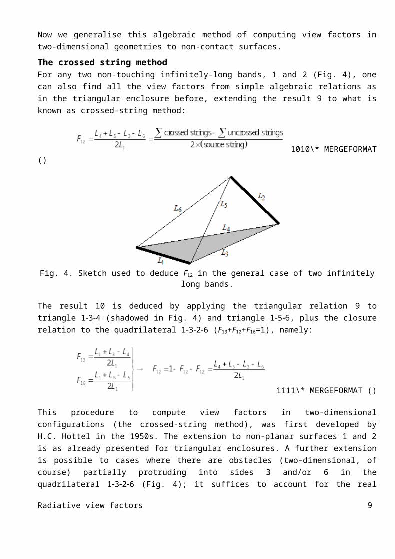
Fig. E1. Sketch used to deduce F12 between two infinitely long parallel cylinders.

View factor with an infinitesimal surface: the unit-sphere and the hemicube methods

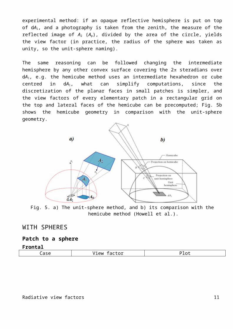
The view factor from an infinitesimal surface dA1 to a finite surface A2, F12=cos(1)d12/, shows that it is the same for any surface subtending a slid angle 12 in the direction 1. Hence, a convenient way to compute F12, first proposed by Nusselt in 1928, is to find the conical projection of A2 on a sphere of arbitrary radius r centred on dA1 (this projection has the same 12), and then project this spherical patch on the base plane containing dA1, as sketched in Fig. 5a (the conical projection on the sphere is As, and its normal projection on the base plane is Ap). The view factor F12 is therefore the fraction of the circle occupied by Ap, i.e. F12=Ap/(r2). This was originally an experimental method: if an opaque reflective hemisphere is put on top of dA1, and a photography is taken from the zenith, the measure of the reflected image of A2 (Ap), divided by the area of the circle, yields the view factor (in practice, the radius of the sphere was taken as unity, so the unit-sphere naming).

The same reasoning can be followed changing the intermediate hemisphere by any other convex surface covering the 2 steradians over dA1, e.g. the hemicube method uses an intermediate hexahedron or cube centred in dA1, what can simplify computations, since the discretization of the planar faces in small patches is simpler, and the view factors of every elementary patch in a rectangular grid on the top and lateral faces of the hemicube can be precomputed; Fig. 5b shows the hemicube geometry in comparison with the unit-sphere geometry.


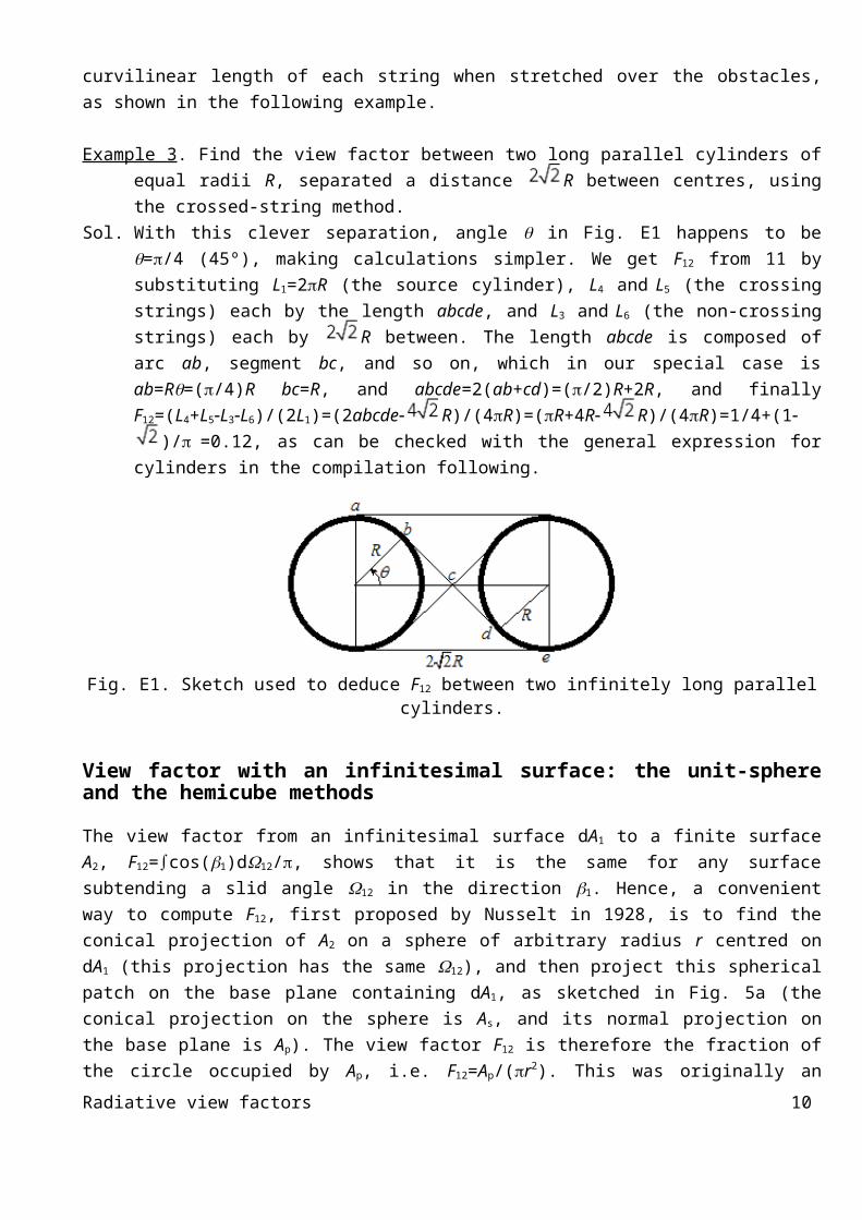
Fig. 5. a) The unit-sphere method, and b) its comparison with the hemicube method (Howell et al.).

WITH SPHERES

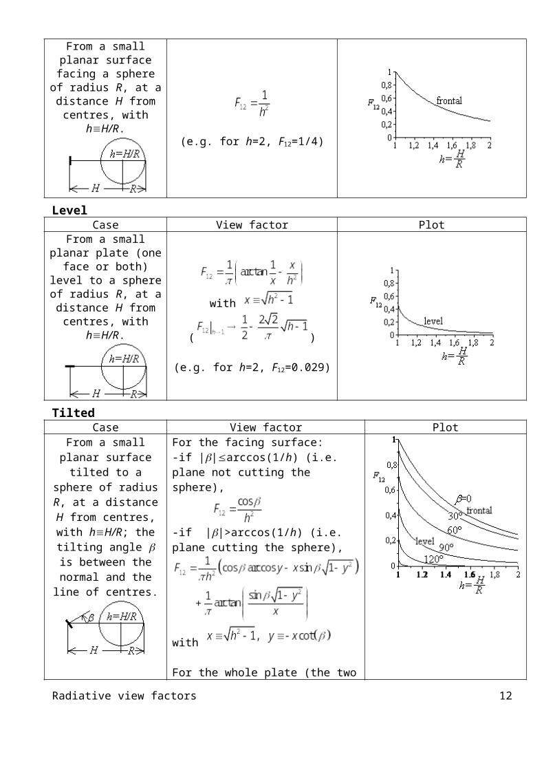
Patch to a sphereFrontal

Case View factor PlotFrom a small planar

surface facing a sphere of radius R, at a distance H

from centres, with hH/R.

(e.g. for h=2, F12=1/4)

LevelCase View factor Plot

From a small planar plate (one face or both) level

to a sphere of radius R, at a distance H from

centres, with hH/R.with

( )

(e.g. for h=2, F12=0.029)

TiltedCase View factor Plot

From a small planar surface tilted to a sphere of radius R, at a distance

H from centres, with hH/R; the tilting angle is between the normal and the line of centres.

For the facing surface:-if ||arccos(1/h) (i.e. plane not cutting the sphere),

-if ||>arccos(1/h) (i.e. plane cutting the sphere),

with

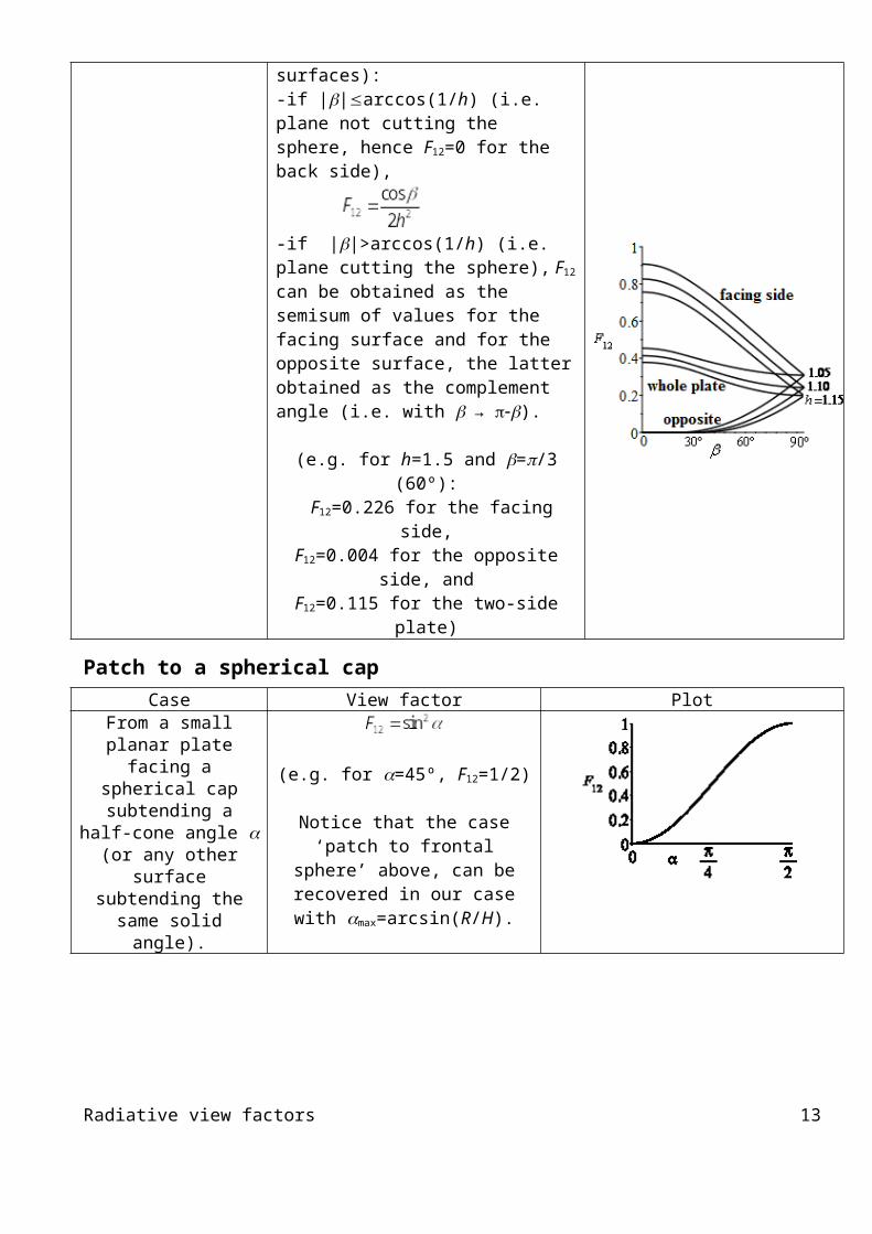
For the whole plate (the two surfaces):


-if ||arccos(1/h) (i.e. plane not cutting the sphere, hence F12=0 for the back side),

-if ||>arccos(1/h) (i.e. plane cutting the sphere), F12 can be obtained as the semisum of values for the facing surface and for the opposite surface, the latter obtained as the complement angle (i.e. with → ).

(e.g. for h=1.5 and =/3 (60º): F12=0.226 for the facing side,

F12=0.004 for the opposite side, andF12=0.115 for the two-side plate)

Patch to a spherical capCase View factor Plot

From a small planar plate facing a spherical cap subtending a half-cone angle (or any other

surface subtending the same solid angle).

(e.g. for =45º, F12=1/2)

Notice that the case ‘patch to frontal sphere’ above, can be recovered in

our case with max=arcsin(R/H).

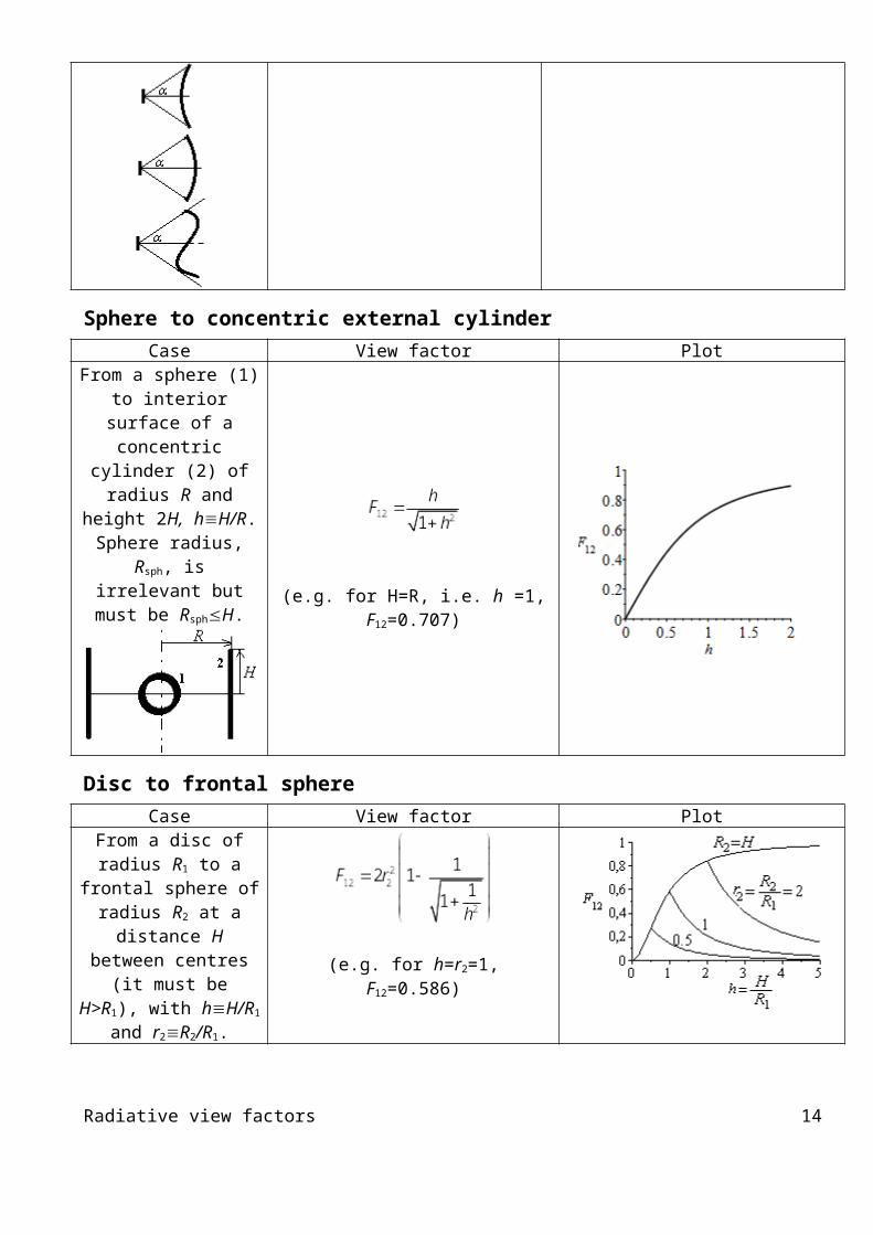
Sphere to concentric external cylinderCase View factor Plot

From a sphere (1) to interior surface of a

concentric cylinder (2) of radius R and height 2H, hH/R. Sphere radius, Rsph, is irrelevant but

must be RsphH.

(e.g. for H=R, i.e. h =1, F12=0.707)


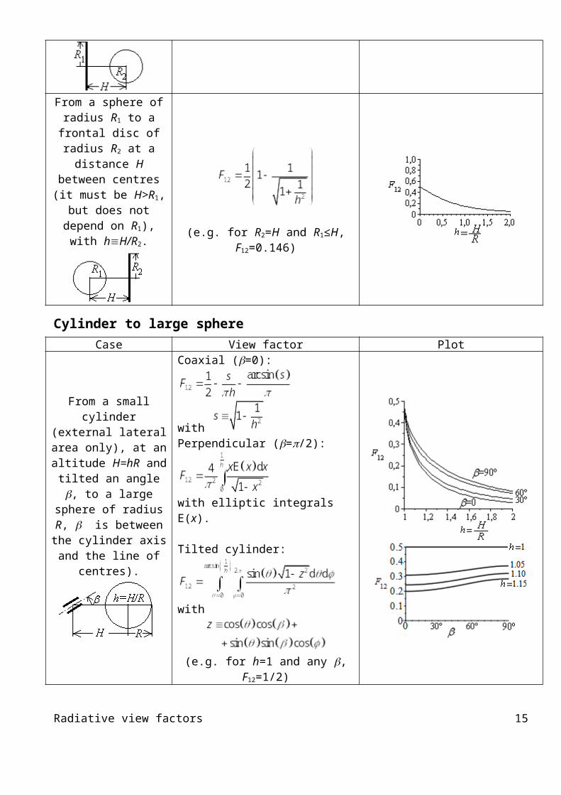
Disc to frontal sphereCase View factor Plot

From a disc of radius R1

to a frontal sphere of radius R2 at a distance H between centres (it must be H>R1), with hH/R1

and r2R2/R1.

(e.g. for h=r2=1, F12=0.586)

From a sphere of radius R1 to a frontal disc of

radius R2 at a distance H between centres (it must be H>R1, but does not depend on R1), with

hH/R2.

(e.g. for R2=H and R1≤H, F12=0.146)

Cylinder to large sphereCase View factor Plot

From a small cylinder (external lateral area only), at an altitude

H=hR and tilted an angle , to a large sphere of radius R, is between

the cylinder axis and the line of centres).

Coaxial (=0):

with Perpendicular (=/2):

with elliptic integrals E(x).

Tilted cylinder:


with

(e.g. for h=1 and any , F12=1/2)

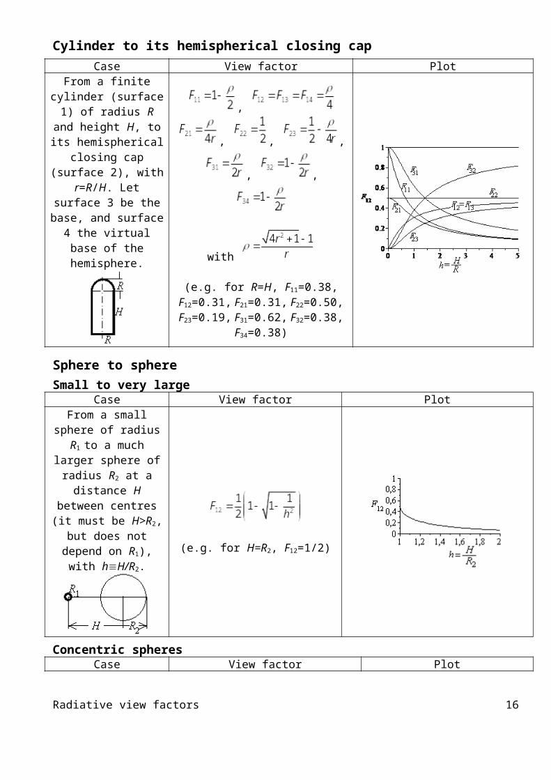
Cylinder to its hemispherical closing capCase View factor Plot

From a finite cylinder (surface 1) of radius R

and height H, to its hemispherical closing cap (surface 2), with

r=R/H. Let surface 3 be the base, and surface 4 the virtual base of the

hemisphere.

,

, , ,

, ,

with

(e.g. for R=H, F11=0.38, F12=0.31, F21=0.31, F22=0.50, F23=0.19, F31=0.62, F32=0.38, F34=0.38)

Sphere to sphereSmall to very large

Case View factor PlotFrom a small sphere of

radius R1 to a much larger sphere of radius R2 at a

distance H between centres (it must be H>R2, but does not depend on

R1), with hH/R2.(e.g. for H=R2, F12=1/2)

Concentric spheresCase View factor Plot


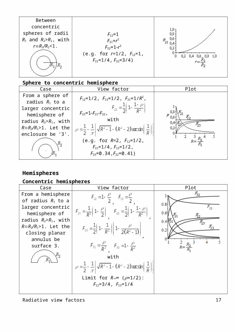
Between concentric spheres of radii R1 and R2>R1, with rR1/R2<1. F12=1

F21=r2

F22=1r2

(e.g. for r=1/2, F12=1, F21=1/4, F22=3/4)

Sphere to concentric hemisphereCase View factor Plot

From a sphere of radius R1 to a larger concentric

hemisphere of radius R2>R1, with RR2/R1>1. Let the enclosure be ‘3’.

F12=1/2, F13=1/2, F21=1/R2,

F23=1F21F22, with

(e.g. for R=2, F12=1/2, F21=1/4, F13=1/2, F23=0.34,F22=0.41)

HemispheresConcentric hemispheres

Case View factor Plot

From a hemisphere of radius R1 to a larger

concentric hemisphere of radius R2>R1, with

RR2/R1>1. Let the closing planar annulus be

surface 3.

, , ,

,

,

, with

Limit for R→∞ (=1/2): F12=3/4, F13=1/4

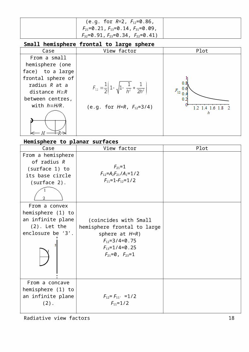
(e.g. for R=2, F12=0.86, F21=0.21, F13=0.14, F31=0.09, F32=0.91, F23=0.34,

F22=0.41)

Small hemisphere frontal to large sphereCase View factor Plot


From a small hemisphere (one face) to a large

frontal sphere of radius R at a distance HR

between centres, with hH/R.

(e.g. for H=R, F12=3/4)

Hemisphere to planar surfacesCase View factor Plot

From a hemisphere of radius R (surface 1) to its

base circle (surface 2).F21=1

F12=A2F21/A1=1/2F11=1F12=1/2

From a convex hemisphere (1) to an

infinite plane (2). Let the enclosure be ‘3’. (coincides with Small hemisphere

frontal to large sphere at H=R)F12=3/4=0.75F13=1/4=0.25F21=0, F23=1

From a concave hemisphere (1) to an

infinite plane (2).

F12= F11’ =1/2F11=1/2

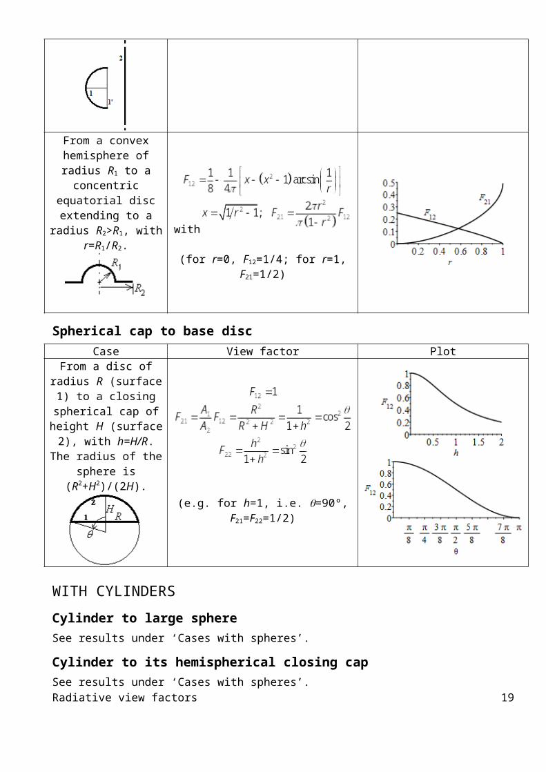
From a convex hemisphere of radius R1

to a concentric equatorial disc extending to a radius

R2>R1, with r=R1/R2.

with

(for r=0, F12=1/4; for r=1, F21=1/2)


Spherical cap to base discCase View factor Plot

From a disc of radius R (surface 1) to a closing

spherical cap of height H (surface 2), with h=H/R. The radius of the sphere

is (R2+H2)/(2H).

(e.g. for h=1, i.e. =90º, F21=F22=1/2)

WITH CYLINDERS

Cylinder to large sphereSee results under ‘Cases with spheres’.

Cylinder to its hemispherical closing capSee results under ‘Cases with spheres’.

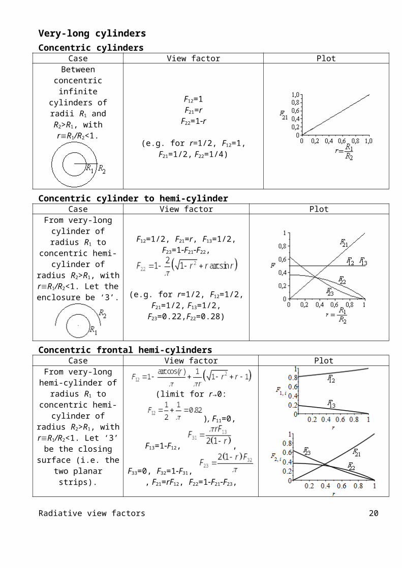
Very-long cylindersConcentric cylinders

Case View factor PlotBetween concentric

infinite cylinders of radii R1 and R2>R1, with

rR1/R2<1.F12=1F21=r

F22=1r

(e.g. for r=1/2, F12=1, F21=1/2, F22=1/4)

Concentric cylinder to hemi-cylinderCase View factor Plot


From very-long cylinder of radius R1 to concentric hemi-cylinder of radius R2>R1, with rR1/R2<1. Let the enclosure be ‘3’.

F12=1/2, F21=r, F13=1/2, F23=1F21F22,

(e.g. for r=1/2, F12=1/2, F21=1/2, F13=1/2, F23=0.22,F22=0.28)

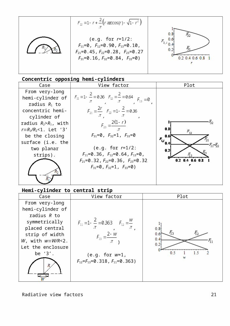
Concentric frontal hemi-cylindersCase View factor Plot

From very-long hemi-cylinder of radius R1 to

concentric hemi-cylinder of radius R2>R1, with

rR1/R2<1. Let ‘3’ be the closing surface (i.e. the

two planar strips).

(limit for r→0: ),

F11=0, F13=1F12, ,

F33=0, F32=1F31, , F21=rF12, F22=1F21F23,

(e.g. for r=1/2:F11=0, F12=0.90, F13=0.10,

F21=0.45, F22=0.28, F23=0.27F31=0.16, F32=0.84, F33=0)

Concentric opposing hemi-cylindersCase View factor Plot

From very-long hemi-cylinder of radius R1 to

concentric hemi-cylinder of radius R2>R1, with

rR1/R2<1. Let ‘3’ be the closing surface (i.e. the

two planar strips).

, , ,

, , F31=0, F32=1, F33=0

(e.g. for r=1/2:F11=0.36, F12=0.64, F13=0,

F21=0.32, F22=0.36, F23=0.32F31=0, F32=1, F33=0)


Hemi-cylinder to central stripCase View factor Plot

From very-long hemi-cylinder of radius R to symmetrically placed

central strip of width W, with wW/R<2. Let the

enclosure be ‘3’.

, ,

)

(e.g. for w=1, F12=F13=0.318, F11=0.363)

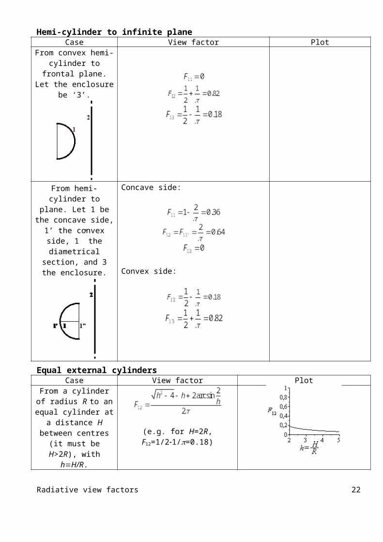
Hemi-cylinder to infinite planeCase View factor Plot

From convex hemi-cylinder to frontal plane. Let the enclosure be ‘3’.

From hemi-cylinder to plane. Let 1 be the

concave side, 1’ the convex side, 1” the

diametrical section, and 3 the enclosure.

Concave side:

Convex side:

Equal external cylindersCase View factor Plot


From a cylinder of radius R to an equal cylinder at

a distance H between centres (it must be

H>2R), with hH/R.

Note. See the crossing-string method, above.

(e.g. for H=2R, F12=1/21/=0.18)

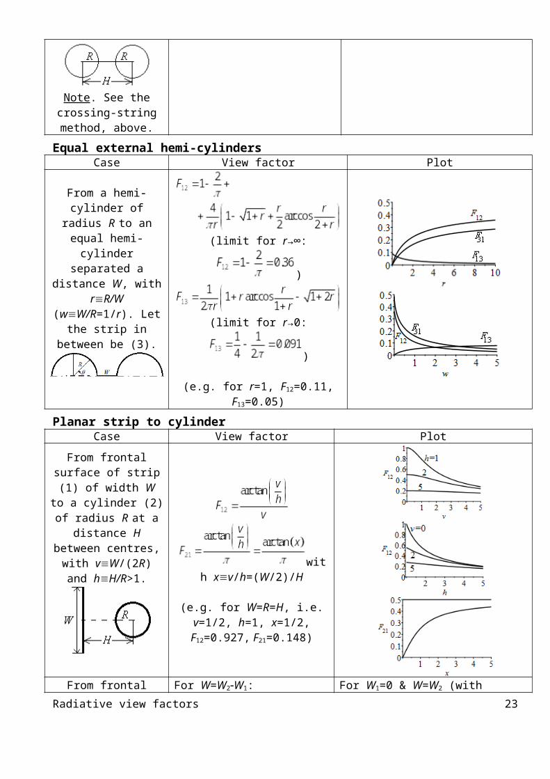
Equal external hemi-cylindersCase View factor Plot

From a hemi-cylinder of radius R to an equal

hemi-cylinder separated a distance W, with

rR/W (wW/R=1/r). Let the strip in between

be (3).

(limit for r→∞: )

(limit for r→0: )

(e.g. for r=1, F12=0.11, F13=0.05)

Planar strip to cylinderCase View factor Plot

From frontal surface of strip (1) of width W to a

cylinder (2) of radius R at a distance H between

centres, with vW/(2R) and hH/R>1.

with xv/h=(W/2)/H

(e.g. for W=R=H, i.e. v=1/2, h=1, x=1/2, F12=0.927, F21=0.148)

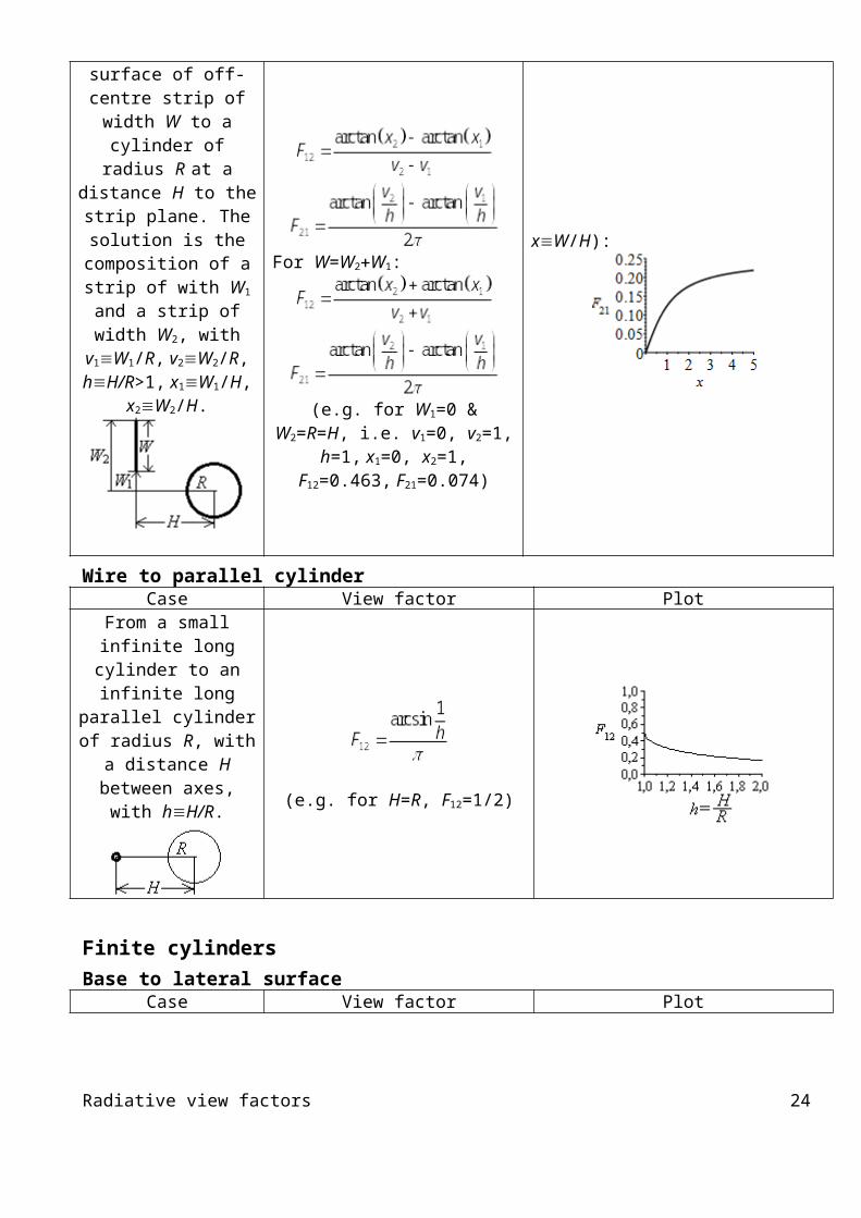
From frontal surface of For W=W2W1: For W1=0 & W=W2 (with xW/H):Radiative view factors 19

off-centre strip of width W to a cylinder of radius R at a distance H to the

strip plane. The solution is the composition of a strip of with W1 and a strip of width W2, with

v1W1/R, v2W2/R, hH/R>1, x1W1/H,

x2W2/H.

For W=W2 W1:

(e.g. for W1=0 & W2=R=H, i.e. v1=0, v2=1, h=1, x1=0, x2=1,

F12=0.463, F21=0.074)

Wire to parallel cylinder Case View factor Plot

From a small infinite long cylinder to an

infinite long parallel cylinder of radius R, with

a distance H between axes, with hH/R.

(e.g. for H=R, F12=1/2)

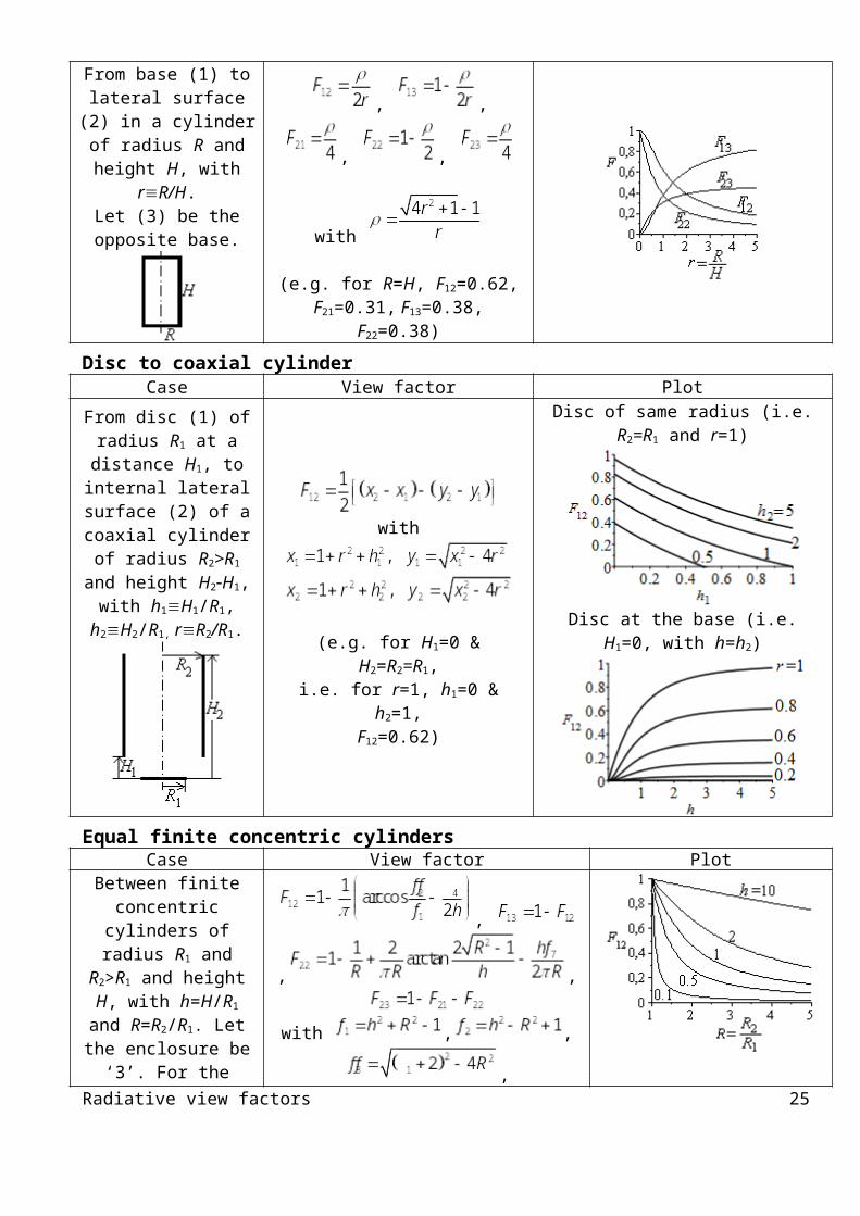
Finite cylindersBase to lateral surface


From base (1) to lateral surface (2) in a cylinder of radius R and height H,

with rR/H.Let (3) be the opposite

base.

, ,

, ,

with

(e.g. for R=H, F12=0.62, F21=0.31, F13=0.38, F22=0.38)

Disc to coaxial cylinder Case View factor Plot


From disc (1) of radius R1 at a distance H1, to internal lateral surface

(2) of a coaxial cylinder of radius R2>R1 and height H2H1, with

h1H1/R1, h2H2/R1,

rR2/R1.

with

(e.g. for H1=0 & H2=R2=R1,i.e. for r=1, h1=0 & h2=1,

F12=0.62)

Disc of same radius (i.e. R2=R1 and r=1)

Disc at the base (i.e. H1=0, with h=h2)

Equal finite concentric cylindersCase View factor Plot

Between finite concentric cylinders of radius R1 and R2>R1 and height H, with h=H/R1 and R=R2/R1. Let the enclosure be ‘3’. For

the inside of ‘1’, see previous case.

, ,

,

with , ,

,

,

, ,

(e.g. for R2=2R1 and H=2R1, F12=0.64, F21=0.34, F13=0.33, F23=0.43, F22=0.23)

Outer surface of cylinder to annular disc joining the base Case View factor Plot


From external lateral surface (1) of a cylinder of radius R1 and height H, to annular disc of

radius R2, with rR1/R2, hH/R2.

,

with , ,

(e.g. for R2=2R1=2H, i.e. r=h=1/2, F12=0.268, F21=0.178)

Cylindrical rod to coaxial disc at one end Case View factor Plot

Thin rod (1) of height H, to concentric disc (2) of radius R placed at one

end, with hH/R.,

(e.g. for R=H, i.e. h=1, F12=1/4)

WITH PLATES AND DISCS

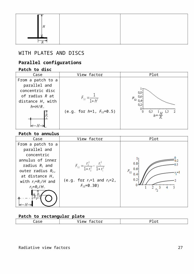
Parallel configurationsPatch to disc

Case View factor PlotFrom a patch to a parallel

and concentric disc of radius R at distance H,

with h=H/R.

(e.g. for h=1, F12=0.5)

Patch to annulusCase View factor Plot


From a patch to a parallel and concentric annulus of inner radius R1 and outer radius R2, at distance H,

with r1=R1/H and r2=R2/H.

(e.g. for r1=1 and r2=2, F12=0.30)

Patch to rectangular plateCase View factor Plot

From small planar patch pointing to a corner of a rectangular plate of sides H and W at a separation

L, with h=H/L and w=W/L. with and

(e.g. for W=H=L, F12=0.139)

Equal square platesCase View factor Plot

Between two identical parallel square plates of side L and separation H,

with w=W/H. with and

(e.g. for W=H, F12=0.1998)

Equal rectangular platesCase View factor Plot

Between parallel equal rectangular plates of size

W1·W2 separated a distance H, with x=W1/H

and y=W2/H.

with and

(e.g. for x=y=1, F12=0.1998)


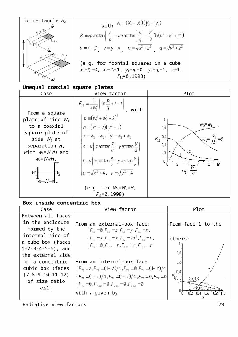
Rectangle to rectangleCase View factor Plot

From rectangle A1 in parallel plane to

rectangle A2.

with

, , ,

(e.g. for frontal squares in a cube:x1=1=0, x2=2=1, y1=1=0, y2=2=1, z=1, F12=0.1998)

Unequal coaxial square platesCase View factor Plot

From a square plate of side W1 to a coaxial

square plate of side W2 at separation H, with

w1=W1/H and w2=W2/H.

, with

(e.g. for W1=W2=H, F12=0.1998)

Box inside concentric boxCase View factor Plot

Between all faces in the enclosure formed by the internal side of a cube

box (faces 1-2-3-4-5-6), and the external side of a

concentric cubic box (faces (7-8-9-10-11-12)

of size ratio a1.

From an external-box face:

From an internal-box face:

From face 1 to the others:


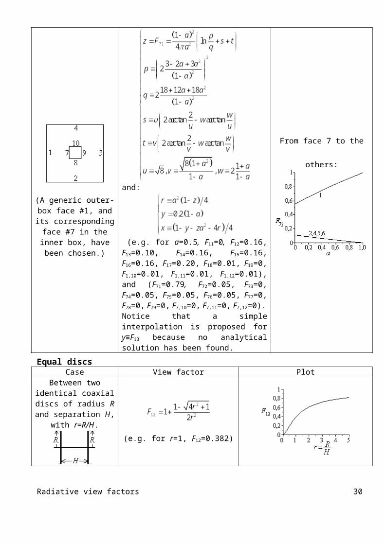
(A generic outer-box face #1, and its corresponding face #7 in the inner box,

have been chosen.)

with z given by:

and:

(e.g. for a=0.5, F11=0, F12=0.16, F13=0.10, F14=0.16, F15=0.16, F16=0.16, F17=0.20, F18=0.01, F19=0, F1,10=0.01, F1,11=0.01, F1,12=0.01), and (F71=0.79, F72=0.05, F73=0, F74=0.05, F75=0.05, F76=0.05, F77=0, F78=0, F79=0, F7,10=0, F7,11=0, F7,12=0).Notice that a simple interpolation is proposed for y≡F13 because no analytical solution has been found.

From face 7 to the others:

Equal discsCase View factor Plot

Between two identical coaxial discs of radius R and separation H, with

r=R/H.

(e.g. for r=1, F12=0.382)

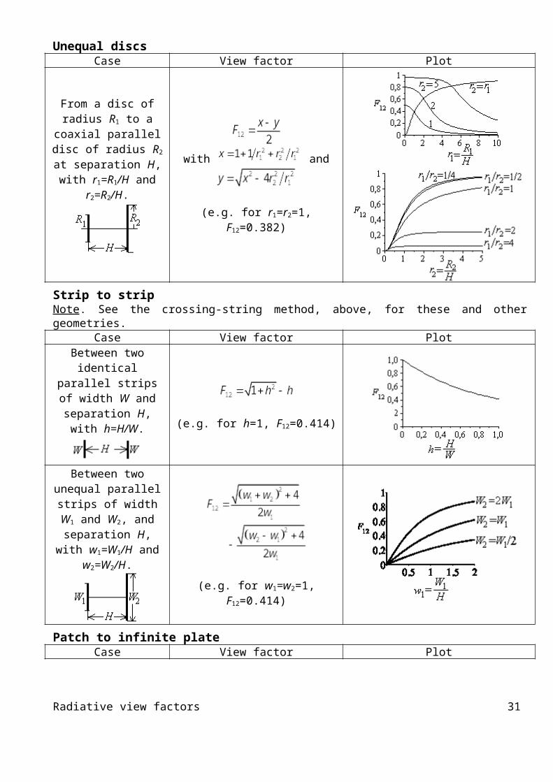
Unequal discsCase View factor Plot


From a disc of radius R1

to a coaxial parallel disc of radius R2 at separation

H, with r1=R1/H and r2=R2/H. with and

(e.g. for r1=r2=1, F12=0.382)

Strip to stripNote. See the crossing-string method, above, for these and other geometries.


Between two identical parallel strips of width W

and separation H, with h=H/W.

(e.g. for h=1, F12=0.414)

Between two unequal parallel strips of width

W1 and W2, and separation H, with

w1=W1/H and w2=W2/H.

(e.g. for w1=w2=1, F12=0.414)

Patch to infinite plateCase View factor Plot

From a finite planar plate at a distance H to an

infinite plane, tilted an angle .

Front side:

Back side:

(e.g. for =/4 (45º), F12,front=0.854, F12,back=0.146)


Perpendicular configurationsPatch to rectangular plate

Case View factor PlotFrom small planar patch

at 90º to rectangular plate of sides H and W at a

separation L, with h=H/W and ℓ=L/W.

with

(e.g. for W=H=L, F12=0.124)

Square plate to rectangular plate Case View factor Plot

From a square plate of with W to an adjacent rectangles at 90º, of

height H, with h=H/W.with and

(e.g. for h=→∞, F12=→1/4,for h=1, F12=0.20004,for h=1/2, F12=0.146)

Rectangular plate to equal rectangular plate Case View factor Plot

Between adjacent equal rectangles at 90º, of

height H and width L, with h=H/L.

with and

(e.g. for h=1, F12=0.20004)

Rectangular plate to unequal rectangular plate Case View factor Plot


From a horizontal rectangle of W·L to

adjacent vertical rectangle of H·L, with

h=H/L and w=W/L.

with ,

,

(e.g. for h=w=1, F12=0.20004)From non-adjacent

rectangles, the solution can be found with view-factor algebra as shown

here

Rectangle to rectangleCase View factor Plot

From rectangle A1 at 90º to rectangle A2 (mind it is

singular if x1=1=0).with

,

(e.g. for squares touching:x1=1=10-6, x2=2=1, y1=1=0, y2=2=1, F12=0.20004)

Strip to stripNote. See the crossing-string method, above, for these and other geometries.



Adjacent long strips at 90º, the first (1) of width W and the second (2) of width H, with h=H/W.

(e.g. )

Cylindrical rod to coaxial disc at tone end (See it under ‘Cylinders’.)

Tilted strip configurationsNote. See the crossing-string method, above, for these and other geometries.

Equal adjacent stripsCase View factor Plot

Adjacent equal long strips at an angle .

(e.g. )

Triangular prismCase View factor Plot

Between two sides, 1 and 2, of an infinite long

triangular prism of sides L1, L2 and L3 , with

h=L2/L1 and being the angle between sides 1

and 2.

(e.g. for h=1 and =/2, F12=0.293)

NUMERICAL COMPUTATION

Several numerical methods may be applied to compute view factors, i.e. to perform the integration implied in 3 from the general expression 2. Perhaps the simpler to program is the random estimation (Monte Carlo method), where the integrand in 3 is evaluated at N random quadruples, (ci1, ci2, ci3, ci4) for i=1..N, where a coordinates pair (e.g. ci1, ci2) refer to a point in one of the surfaces, and the other pair (ci3, ci4) to a point in the other surface. The view factor F12 from surface A1 to surface A2 is approximated by:

1212\* MERGEFORMAT ()


where the argument in the sum is evaluated at each ray i of coordinates (ci1, ci2, ci3, ci4).

Example 4. Compute the view factor from vertical rectangle of height H=0.1 m and depth L=0.8 m, towards an adjacent horizontal rectangle of W=0.4 m width and the same depth. Use the Monte Carlo method, and compare with the analytical result.

Sol. The analytical result is obtained from the compilation above for the case of ‘With plates and discs / Perpendicular configurations / Rectangular plate to unequal rectangular plate’, obtaining, for h=H/L=0.1/0.8=0.125 and w=W/L=0.4/0.8=0.5 the analytical value F12=0.4014 (mind that we want the view factor from the vertical to the horizontal plate, and what is compiled is the opposite, so that a reciprocity relation is to be applied).For the numerical computation, we start by setting the argument of the sum in 12 explicitly in terms of the coordinates (ci1, ci2, ci3, ci4) to be used; in our case, Cartesian coordinates (xi, yi, zi, y’i) such that (xi, yi) define a point in surface 1, and (zi, y’i) a point in surface 2. With that choice, cos1=z/r12, cos2=x/r12, and , so that:

where fi is the value of the function at a random quadruple (xi, yi, zi, y’i). A Matlab coding may be:W=0.4; L=0.8; H=0.1; N=1024; %Data, and number of rays to be usedf= @(z,y1,x,y2) (1/pi)*x.*z./(x.^2+z.^2+(y2-y1).^2).^2; %Defines the functionfor i=1:N fi(i)=f(rand*H, rand*L, rand*W, rand*L);end; %Computes its valuesF12=(W*L/N)*sum(fi) %View factor estimation

Running this code three times (it takes about 0.01 s in a PC, for N=1024), one may obtain for F12 the three values 0.36, 0.42, and 0.70, but increasing N increases accuracy, as shown in Fig. E4.

Fig. E4 Geometry for this example (with notation used), and results of the F12-computation with a number N=2in of random quadruplets (e.g. N=210=1024 for in=10); three runs are plotted, with the mean in black.


REFERENCESHowell, J.R., “A catalog of radiation configuration factors”, McGraw-Hill, 1982. (web.)Siegel, R., Howell, J.R., Thermal Radiation Heat Transfer, Taylor & Francis, 2002.

Back to Spacecraft Thermal Control


http://webserver.dmt.upm.es/~isidoro/tc3/Spacecraft%20Thermal%20Control.pdf

http://www.thermalradiation.net/tablecon.html

Documents

Radiation View factors - ¡Bienvenidos! — Portal …webserver.dmt.upm.es/~isidoro/tc3/Radiation View factors... · Web viewView factor definition2 View factor algebra3 View factors