IEEE Transactions on Plasma Science, Vol. PS-6, No. 4, December 1978

RADIATION PHENOMENA OF PLASMA WAVES

PART 2. RADIATION FROM POINT SOURCES

Toshiro OhnumaDepartment of Electrical Engineering

Tohoku UniversitySendai 980, Japan

CONTENTS

1. I ntroductionII. Radiation of plasma waves in an isotropic plasmaIll. Radiation of electrostatic electron waves in an aniso-

tropic plasma111-1. Radiation of electron plasma waves111-2. Radiation of electron cyclotron harmonic waves111-3. Radiation of upper hybrid waves

IV. Radiation of electrostatic ion waves in an anisotropicplasma

IV-1. Radiation of ion plasma waves-low frequencyresonance cone-

IV-2. Radiation of electrostatic ion cyclotron waves(neutralized ion Bernstein waves)

IV-3. Radiation of pure ion Bernstein wavesI V-4. Radiation of lower hybrid waves

V. Radiation of electromagnetic electron waves in an

anisotropic plasmaV-1. Radiation of whistler and electron cyclotron

wavesV-2. Radiation of quasi-static electron waves-high

frequency resonance cone-

V-3. Reflection of high frequency resonance cone

VI. Radiation of electromagnetic ion waves in an aniso-tropic plasma

VII. Radiation in a plasma stream

I. INTRODUCTION

Radiation from a point source is a fundamental problemin radiation phenomena. The investigations on this problemgive many important effects which are characteristic for each

plasma mode and gives some insight into the problem of

radiation from finite sources. Therefore, the author wants

to explain this problem in detail. The definition of a pointsource that will be used is that the source size is much smallerthan the wave length of the electromagnetic or any plasmawave; an infinitesimal source is exactly called a point source.

When one considers radiation from a point source, it isvery convenient to investigate phase, group, and ray velocitysurfaces. Especially, group and ray velocity surfaces are impor-

tani because the former indicates the propagation of wave-packets from a point source and because the latter showsthe wave fronts radiated from the point source. In part 2,radiation from point sources, phase, group, and ray velocitysurfaces for many plasma modes are presented. Furthermore,experimental data on radiation from point sources are in-cluded. In Figure 1, phase velocity surfaces for plasma wavesand slow electromagnetic waves are indicated [1] . In additionto the original phase velocity surfaces, plasma modes whichwill be explained in this report are included in the figure,and the frequency-boundary at the ion plasma frequencyis added on the abscissa.

Experimentally, Fisher and Gould (1969, 1971) observedthe high frequency resonance cone [2],[3]. This observationmay be the first epoch-making experiment on radiation froma point source. Gonfalone (1972) observed clear fine struc-

tures due to electron thermal motion on an after-glow plasma[4]. Furthermore, Gonfalone et al. (1973, 1974) reportedan observation of potential patterns of electron Bernstein

waves (electrostatic electron cyclotron waves) radiated from a

point source [5] ,[6] . The ray velocity surfaces of the electronBernstein waves was confirmed by Ohnuma et al. (1977)[7]. Three-dimensional whistler waves radiated from a mag-netic loop and the relation of the whistler wave to the reso-

nance cone were observed by Boswell (1975) [8]. Further-

more, Boswell and Giles (1976) investigated the parametricinstability inside the high frequency resenance cone [9] .The transient response of a cold anisotropic plasma to a point

0093-3813/78/1200-0478$00.75 (© 1978 IEEE

478

to r s iona 1 (68)'Alfven waves

compressional (69))

ion waves

(low frequencyresonance cones, 30)

IX - - r

xlI

I

I.

UL=O

electrostatic ioncyclotron waves (37)

21ion Bernstein neutralized

wavesI L pure (39)

ower

whistler waves (47) IL yLJ"". r wave

J0=OO I ion v

oblique electroplasma modes ""(thermal

/\ effectsfor resonance

cones, 58)

s (40)vave s (40)

Ur =0

electron Bernsteinwave s (16)1

ion waves (6)

(thermal effects for Z-moderesonance cones, 59)

y "I iuf

waves (25) 1

Figure 1. Phase velocity surface of slow electromagnetic modes and plasma modes [1]. In addition, the fre-quency's boundary at the ion plasma frequency f and several names and figure numbers of modes whichare explained in this report are inserted.

479

IB0 t

.x

f .ci

C1.

fce

electr

I

I

x

'k xrl-% -r i rl1(

pe

source using an impulse excitation has been reported by

Simonutti (1976) [10]. Stenzel (1976) investigated wave

fronts of whistler waves in three dimensions [111 . Further-

more, Stenzel (1977) observed obliquely unstable whistler

waves in an electron-beam plasma system [12]. Spatial varia-

tions of the resonance cone was observed clearly by Ohnuma

(1977, Sec. V-2 of this report). Furthermore, the reflection

of the resonance cone near the fpe-layer was confirmed by

Ohnuma and Lembege (1977, V-3) [13]. For an electron

plasma wave, Ohmori et al. (1976) studied this mode in

detail in three dimensions [14].In the low frequency region, Ohnuma et al. (1975)

confirmed the radiation characteristics of ion waves in a weak-

ly magnetized plasma [15]. He observed the phase velocity

surfaces and the amplitude pattern of ion waves radiated

from a point source. Furthermore, Ohnuma et al. (1976)

observed obliquely unstable ion waves radiated from a point

source in an ion-beam plasma system [16].For the frequency region near the lower hybrid fre-

quency, Ohnuma et al. (1977) investigated radiation of elec-

trostatic waves from a point source [17]. He investigated the

ion wave and the lower hybrid wave by investigating those

ray velocity surfaces, namely, wave fronts radiated from a

point source.During these investigations, Hirose et al. (1970) investi-

gated oblique propagation of ion waves near the ion cyclotronfrequency although the anisotropy was not clearly considered

[18]. With regard to the electrostatic ion wave, Ohnuma

et al. (1976) observed the low frequency resonance cone

[19]. Furthermore, they investigated the relation of the

resonance cone to ion waves radiated from a point source

[20]. Belan (1976) also observed this low frequency reso-

nance cone [21].

11. RADIATION OF PLASMA WAVES FROM

A POINT SOURCE IN AN ISOTROPIC PLASMA

2 2Ce =3V /2.

Ion plasma wave:

2=

2 3k2 2

1±+k6,/k 2 i (3)

k2 ik(2kY1 =E 2ek i ( )± zt( e) . (4)

2k kV 2k2 kV.e 1

Electromagnetic wave:

2 2 2 2W = W + k c

pe (5)

Those typical dispersion curves are indicated in Figure 2.

Cpe

0

EL ECTROMAG,NE TICWAVE

; ELECTRONPLASMA WAVE

P, W

PLASMA WVE

KDe K

Figure 2. Three independent modes in an isotropic plasma.

Concerning the radiation of these modes, the fundamentalresults are indicated in V-3 of Part 1 of this series. As shown

in Eqs. 1-(20) and 1-(24), the radiation field from a pointsource for electron and ion plasma waves is given in the

following form;

In an isotropic plasma, there are three independentmodes, an electron plasma wave, an ion plasma wave, and an

electromagnetic wave. The simple dispersion relations for

these modes are given as follow;Electron plasma wave:

2 2 22Uj =CO +k C ( fluid ) (1)

pe e

k= 2 7(k ) '1=2k2 V(kinetic) (2)

ikR - iut

X (R) o' Re (6)

where k is the wave number of the electron or ion plasmawaves. This indicates an outgoing spherical wave from a pointsource and has a geometrical damping of 1/R for the wave

amplitude. Those spherical wave fronts are shown in Figure 3.

In an isotropic plasma, the direction of the group velocity is

the same as that of the phase velocity; the ray velocity sur-

face is the same as the phase velocity surface.

For the radiation from a point dipole of IP = pz, the

k2 =202 /V2, V2=2T /mDe- p e e e e

480

WAVE FRONTS LK

IK

t

-IK

Figure 3. Wave fronts of a spherical wave.

far field of the electric field can be obtained from Eq. 1-(33)with R -+ oo;

IE(R) = IEt(R) +E±(R) (7)

pk . eiktR itA2 2 sinG 9

t 4¢eO 1 - pe/UJ)R

pkf eikIR-iwt A

IE (R)=- 2 cos9 r

1 4Tllo( - WJe/p R

where IEt(R) and 1E1 (R) are the fields of the electromagneticwave and of the electron plasma wave radiated from a pointdipole, respectively. Although it is not included in Eq. 7,the field of the ion wave has a similar form to that of theelectron plasma wave. The field intensity patterns are indi-cated in Figure 4 for the electromagnetic wave (EM) and theelectron plasma wave (EP). The electron plasma wave has a

peak amplitude in the direction of the dipole moment. On theother hand, the electromagnetic waves has a peak amplitudein the direction perpendicular to the dipole moment.

As a typical experimental result, radiation of an ionplasma wave from a point source by Ohnuma et al. (1975)(151 is presented here. The experiments were performed ina vacuum chamber 32 cm in diameter and 160 cm in length.The schematical experimental setup is indicated in Figure 5.The typical plasma parameter values were No 109 cmf3for the plasma density and Te - 1.5 - 2.0 eV for the electrontemperature at an argon pressure P t 6 x 10 -4 Torr. Theexcitation and detection of ion waves were performed with a

small probe and a small mesh, respectively. The detector was

movable radially and azimuthally with respect to the exciter.The phase velocity and amplitude of the ion waves observedfor three dimensions are indicated in Figure 6. The typicaloperating frequency for the ion waves was 100 kHz with a

Figure 4. Field intensity patterns of electron plasma wavesand electromagnetic waves radiated from a point dipole inisotropic plasmas. The arrow indicates the direction of thedipole moment.

x -. -

_ _ - _--ot' - 3

E X C T E R

/-

IIT7 H DE AN i)DE

i I ii

Figure 5. Schematical experimental setup for radiation inisotropic and anisotropic plasmas.

wavelength of a few centimeters. In an isotropic plasma(Figure 6a), ion waves are shown to propagate omnidirec-tionally in the phase velocity with equal amplitude. Thisfact is in fair agreement with the theoretical results of Eq. 6,which were drawn with solid and dot-dashed lines in thefigure. In that paper, furthermore, interesting characteristicsof the radiation in a weakly magnetized plasma were reported.Typical data are indicated in Figure 6b. The ion waves in sucha plasma are shown to propagate omnidirectionally witha uniform phase velocity and to be launched along the mag-

netic field with a greatly enhanced amplitude. The resultscould be explained by an excitation mechanism due to oscil-lating current flows to the probe along the magnetic fieldrather than by that due to oscillating point charges.

Ill. RADIATION OF ELECTROSTATIC ELECTRONWAVES IN AN ANISOTROPIC PLASMA

There are two independent modes of electrostatic elec-

481

EM ,

[P

[P

il

.

k2

(a) I8 0

f -100kHz

180A

xiO Cm/soC

4 3

Waveampli tude

Phosevelocity

(b) 8 5.5G 90 4xlocm/sec

f OOkHZ

.2

160 - - 0 -

180 g 0* , 0-, ,|.lo_- ,_______ h

4 2 *#l 2I;#P42 B

Wave 2 Phaseamplitude veloci ty

270 4

Figure 6. Experimental and theoretical phase velocity surfacesand amplitude patterns of ion waves radiated from a pointsource, (a) in isotropic plasmas; and (b) in weak anisotropicplasmas.

tron waves in an anisotropic plasma, namely, the electronplasma mode and the electron cyclotron harmonic mode.The former is sometimes called the Landau mode and hasthe same dispersion relation as that in an isotropic plasmafor the propagation parallel to the magnetic field. The latter is

sometimes called the electron Bernstein wave or the electro-static electron cyclotron wave. This mode includes the upperhybrid wave which can be derived from fluid theory. Thedispersion relation of the electrostatic electron wave in an

anisotropic plasma is given as follows:

1 -

w 2pe

U2 _ 2e222ce 22CL) ce -k Cw2 e

1 - 2ceos 2

W2 2~~~~~1

= 0 , (8)

,, e oe ne)" ~~~~~~(9')

2 2 2 2k E2W//V,V -2TmkDe -2 pe e e e/m e

22 2k1V /2(t) , ). (LL.-nCLT )/kVe e ce ne ce ewhere In(X) and Z(ai) are the modified Bessel function andthe plasma dispersion function, respectively. The schematicaldispersion curves for the propagation parallel and perpendi-cular to the magnetic field are indicated in Figures 7 and 8.

pe

KDe K,lFigure 7. Dispersion curve of electron plasma waves propa-gating parallel to the magnetic field in infinite anisotropicplasmas.

U-

ce5

4WUM

3

2

1

0L

I

,'.~UPERHYBRD

ELECTRON BERNSTEINWAVE

2 4eFigure 8. Typical dispersion curves of electron waves propa-gating perpendicular to the magnetic field.

Figure 7 indicates the dispersion curve for the electron plasmawave and Figure 8 are those for electron cyclotron harmonicwaves.

/k =cos2

482

I1-1. Radiation of Electron Plasma WavesIn order to clarify the radiation phenomena, the wave

number of the electron wave for any direction is first obtained

from the fluid and kinetic dispersion relations Eqs. 8 and 9.Figure 9 indicates that propagation of the electron plasma

velocity surfaces. The difference between those velocitysurfaces is clearly shown. As indicated in 11-2 of part 1, the ray

velocity surface is the wave front of the electron waves radiat-

ed from a point source. The potential of the electron waves

radiated from a point source can be obtained from Eqs.60 and 61 of part 1. The typical wave potential around the

point source is shown in Figure 11 for both cases with the

K

Koe

0 0.2 a4K/KDe

Figure 9. Wave numbers of the electron plasma wave in a polarcoordinate.

wave is localized around the direction of the magnetic field.The typical phase, group, and ray velocity surfaces for this

electron plasma wave are indicated in Figure 10. These are

t I80

V /Ve

C,

2 0

f/fce 0.69

f /fpe I 6

KINETIC

NiP oe

Figure 11. Angular potential pattern of electron plasmawaves radiated from a point source according to fluid andkinetic theories.

fluid and kinetic models. The kinetic potential is much more

localized along the magnetic field than the fluid potential

because of the kinetic damping.In experiments [101 , typical wave fronts of the electron

plasma waves radiated from a point source are indicated in

Figure 12. The typical plasma parameter values were NoIB0

c m

6

2

WAVE'

to. V FRONTS

I6 *-

*.S

a

Figure 10. Phase (V ), group (Vi), and ray (Vr) velocity sur-faces normalized by the electron thermal velocity Ve = (2Te/me)Y2for the electron plasma wave.

2 -

2Exciter

4 6

4 6 cm

obtained for the fluid and kinetic models from the definitions,Eqs. 5 - 7 of part 1. The marks A, B, and C on the phasevelocity surface correspond to those on the group and ray

Figure 12. Experimental and theoretical wave fronts of theelectron plasma wave radiated from a point source for flf =

0.96 and f/f = 1. 17.pe

483

1 2 x 108cmr3,T =4-5eV, fe, 140MHz andf >e Ice cef > fp for the operating frequency. The closed circles andpesolid curves are the experimental results and the theoretical

wave fronts, respectively. From such wave fronts, one can

obtain easily the ray velocity surface. The ray velocity surfaces

are indicated in Figure 13. The experimental ray velocity

IBo I

rayvelocIty

*- .-* * . A.

2 -

=73° Vq A_.4=7 v

f-l34MHzfc= 140MHzfp= 115MHz

*ee_

.

VP

0=-17

ponding theoretical wave-amplitude from kinetic theory.

The experimental angular amplitude is nearly in accord with

the kinetic amplitude.

111-2. Radiation of Electron Cyclotron Harmonic Waves

In this section, three dimensional propagation of the

backward electron Bernstein waves, namely the electron cyclo-

tron harmonic wave or the electrostatic electron cyclotronwave, will be explained. Although Gonfalone et al. first

measured [51 the potential around the probe for the electron

Bernstein wave, the investigations by Ohnuma et al. [7] are

presented in this report because they have studied the ray

velocity surfaces etc. in detail.In Figure 15, typical real (kr) and imaginary (k.) wave

# B.4 2 2 4

X 10 cm/sec

Figure 13. Experimental and theoretical ray velocity surfaces

for the electron plasma wave.

surface is in fair agreement with the theoretical ray velocitysurface. The ray velocity surface is clearly shown to be dif-

ferent from the phase velocity surface. The experimentalamplitude of the electron plasma wave radiated from a pointoscillating source is indicated in Figure 14 with the corres-

30 60 e 90

Figure 14. Experimental wave amplituae of the electron plas-

ma wave radiated from a point source with the corresponding

theoretical potential pattern, R = r/rL.

Figure 15. Wave numbers of the electron cyclotron harmonic

wave (the electron Bernstein wave) in polar coordinates.

numbers of the backward electron Bernstein wave are shown

in polar coordinates. Those of the Landau mode are indicated

because of the frequency f > fpe In Figure 16, the phase

20 15

Ve

fhor o,

IA10 05 0

f/fce=1 30

f/fpe=081

Bernstein

VpVe

0.5 AW0-5 A 10 1-5 2-0

Figure 16. Phase (V ), group (Vg), and ray (Vr) velocity sur-

faces of the electron Bernstein wave.

484

0.4

Q2

1/fce=142f/fpe=1 25

Kr

Landau K

_1

"",-o s r

0 0.2 0.4KPe

S - - w- w.E ;oI ~~~~~- - 1.I _ s _ ~~~~^ _- AI. IA-

y

A

(Vp), group (V ), and ray (V r) velocity surfaces of the elec-

tron Bernstein wave are indicated for typical plasma parametervalues. Only one quarter part of those velocity surfaces are

indicated. The phase velocity surface is restricted to a verynarrow region perpendicular to the magnetic field. Thisindicates that the wave normal of the electron Bernstein waveis nearly perpendicular to the magnetic field. On the otherhand, the corresponding group and ray velocity surfaces ex-tend for wide angular regions. The typical wave fronts of theelectron Bernstein wave which is radiated from a point sourceare indicated in Figure 17. The fronts can be easily obtained

f/fce =1 .2511e f/fpe=0 78

WAVE FRONTS

Figure 17. Wave fronts of the electron Bernstein wave radiatedfrom a point source. Ray direction is in agreement with theobserving direction.

from the ray velocity surface. The ray direction is shownto be different from the direction of the wave normal (1k).

The experimental results in a large space chamber 2 min diameter and 3.5 m in length are presented for a confirma-tion of the theoretical results. The typical parameter valueswere No 4 x 106 cm-3, Te = 2 - 3 eV, fce = 9.3 MHzand fpe > f > fce. The typical dispersion curve, the wavefronts and the ray velocity surface of the electron Bernsteinwave radiated from a small probe are indicated with closedcircles in Figures 18, 19, and 20. The corresponding theore-tical curves are shown with solid curves. Figure 20 clearlyindicates the ray velocity surface of the electron Bernsteinwave. The potential pattern of the electron Bernstein wavewhich was observed around the launcher at a fixed distancefrom the launcher is shown in Figure 21. The peak potentialsarise from the coupling between the electron Bernstein wave

f

1 UpperHybrid Frequency

0 1 2 3

Figure 18. Experimental and theoretical dispersion curvesof the electron Bernstein wave, Te = 2.8 eV.

f/fce=1 .3f/fpe=0.65

Figure 19. Experimental wave fronts of the electron Bernsteinwave with the corresponding theoretical wave fronts. 80:the externally applied magnetic field, IB: the summation ofthe 180 and the terrestrial magnetic field, f = 14.9 MHz.pe

and the quasi-static field. Namely, the peak potential is relateddirectly to the wave fronts as shown in Figure 22. The crosspoints of the wave fronts over the locus of the detectorin Figure 22 are in accord with the peak potential of Figure21. The experimental potential is compared in Figure 23with the theoretical potential pattern which was obtainedfrom a numerical calculation of Eq. 1-(54).

111-3. Radiation of Upper Hybrid WavesFor a frequency larger than an upper hybrid frequency

fuh = )+ f2pe)/2, there exists the forward electron Bernstein

485

C Vr

Vg

cVeAl'

ft

2D ISA 1.0 0.5 /0Exciter

20

15 tf

1D

/1fce 1.5

pe =Q76

VPVe

05 1D 15 210

Figure 20. Experimental ray velocity surface with the cor-

responding ray, phase, and group velocity surfaces. Te =

2.8 eV and NO = 4.2x 106 cmy3.

f e: S.3 Mt4

t.1 1.8MHz

12.0MHz

2.5MHz

12.8MHz30

&

Figure 21. Experimental angular potential patterns of the elec-

tron Bernstein wave radiated from a point source.

wave as shown in Figure 18. In this frequency region, the wave

number which was obtained numerically from Eq. 9 is plotted

in a polar coordinate in Figure 24. The typical phase, group,

and ray velocity surfaces normalized by the electron thermal

velocity Ve = (2T1/m1/2 are indicated in Figure 25 for two

parameter values. These are obtained with a kinetic model.

The velocity surfaces are more complicated than those of the

backward electron Bernstein wave due to the electron thermal

Figure 22. Wave fronts of the electron Bernstein wave radiated

from a point source and the locus of the detector. The posi-

tion of the closed circles are in agreement with the peak po-

tentials of Figure 21.

U)

L-n

c.J

O 30* 60 90°

Figure 23. Experimental and theoretical angular potentialpattern of the electron Bernstein wave radiated from a pointsource. R = r/rL = 40, f/f 1.25 and f/f = 0.93.souce.R=rlr lce=pe

effects.

In the same chamber which was used for the backward

486

IU

tf/tce=1.25f/tpe=0 78

J-90(cm)

Exciter

-~~~~~~~~~~~~~~~~~V ;^----

I

05

IR. (a) s , _observed as shown in Figure 26. The typical argon plasma

AYe "T I wIpe/ Tce AA.J0.4 (b) f / fce =2.46 130

(a) fpe/fce-2.00 10f /kfe =2.26

0.2 f/fce=21 8 V

Kr ~~~~~~~fff=1.4 6-

9Q0 ~~~40 0.2 0.4 0.6

KS'e ~~~~~~~2VP

Figure 24. Wave numbers of t7e upper hybrid wave in polarcoordinates. /i 2 4 6 8 10

ExciterFigure 26. Experimental ray velocity surface of the upper

tlBo fpe/fce=2.00 hybrid wave with the theoretical ray and phase velocityc f /6ce =2.46 surfaces.

parameters were No= 4 x 106 cmr3 and Te = 2 3 eV.

I8 g / |S,D !i? \ The theoretical ray and phase velocity surfaces are indicated2 Ve D with solid lines for the experimental conditions. The experi-

Ve D mental ray velocity surface is in accord with the theoreticalv f iO \ i ray velocity surface.

B 90° IV. RADIATION OF ELECTROSTATIC ION WAVESIN AN ANISOTROPIC PLASMA

L There exists two independent modes of electrostatic ion8 ' fpePpe/fce-=200 waves in an anisotropic plasma, namely, the ion plasm mode

| / e f /fe =2.26 and the ion cyclotron harmonic mode. The former has the4 C same dispersion relation as the ion plasma mode in an aniso-

AB tropic plasma for propagation along the magentic field. The0 90 latter is sometimes called the ion Bernstein wave and includesB 8 16 2

D4/4\ | the lower hybrid wave and the electrostatic ion cyclotron4 t B wave which can be derived from fluid theory. The dispersion

V relation of the electrostatic ion wave in an anisotropic plasma

8 \& is given as C2~x10 1- 2 pe2 2 2

t ~ ~ ~ C (i c e 2 2-kGCCL)e ece- cos

2

Figure 25. Phase (Vp), group (Vg), and ray (V,J velocity sur- 2faces of the upper hybrid waves. pi =0, (10)

(A_-_ _ci 2 2electron Bernstein wave, the experimental ray velocity surface 2 k C ifor the upper hybrid wave radiated from a small probe was 1 Ci 2

CS2

487

zkDr J )c .(c)OI1+ I[+e ;In(X.) .O7.(, J0i j njJ

(11)

where the summation about j is performed for electrons and

ions. The meaning of the symbols are similar to Eq. 9.

Typical dispersion curves for the propagation parallel

(1k//1B0), nearly perpendicular (1k 1 IB0) and perpendicular(ik 1 IBO) to the magnetic field are indicated in Figures 27,28, and 29. Figure 27 indicates the dispersion curve of the

W.pi

Koe

1

0

K1

Figure 27. Schematical dispersion curve of ion waves propa-

gating parallel to the magnetic field, k/lIBo.

7

CU)

CTRCISCTAI:4 1 ON CYCROTRON

3

2 ,' NEUTRALIED,ION BERNSTEIN

0 1 2 3 4 5K.LP

Figure 28. Dispersion curve of ion Bernstein waves propagatingnearly perpendicular to the magnetic field, Ik 1 IBO.

ion plasma wave. Figures 28 and 29 are those of the ion cyclo-tron harmonic waves.

IV-1. Radiation of Ion Plasma Waves-Low FrequencyResonance Cone-

The simple dispersion relation for ion waves in a mag-

PUREION BERNSTEIN

WAVE

2 3 4 5KLPi

Figure 29. Dispersion curve of ion Bernstein waves propagating

perpendicular to the magnetic field, 1k 1 IB .

netized plasma is indicated in Eq. 65 of part 1. From the di-

electric constant of the ion waves, the phase, group, and ray

velocity surfaces can be obtained as shown in Figure 30 for

0.5 0

1t f/fj.zQ.5aB f zfI

FLUID

A

0.5 C

/ Vp /Vs

0.5

Figure 30. Phase (Vp), group (Vg), and ray (Vr) velocitysurfaces of ion waves in anisotropic plasmas from a fluid the-

ory. V5 = (TeImi)', Ti/Te < 1 and f< fci

a frequency lower than the ion cyclotron frequency. The

velocity surfaces are normalized by the ion acoustic velo-

city Vs = (Te/mi)/2. When one uses the kinetic dielectricconstant of Eq. 11, the phase, group, and ray velocity surfaces

of the ion waves are obtained as indicated in Figure 31.

In order to clarify the meaning of those velocity surfaces,the energy flow region from a point source is indicated with

488

w 6-

wci 51

I

D

Vr /Vs

Vg /Vs

T

a5 0

00

1t f/f0f itfB\ KINETIC

* *; Experimental ,Vp /Vs

-; Theoretical

-9w -0.5

Bo

ed

I WaMve Fronts

(U/ (,40.7wp,//05

T / Te -005

Exciter

Figure 31. Phase, group, and ray velocity surfaces of ion wavesin anisotropic plasmas from kinetic theory, f< fc.

Figure 33. Experimental wave fronts of ion waves radiatedfrom a point source in anisotropic plasmas. f < fci Solidcurves are the theoretical wave fronts.

a shaded region in Figure 32. The edge cone angle of the

10

(Ji ,/ U.r = 5T, I Te =005M /U)C= s

----

Figure 32. Phase, group, and ray velocity surfaces of ion waves

in anisotropic plasmas from kinetic theory, f < fcp The energy

flow is localized inside the shaded region.

group velocity surface is in accord with the boundary for thepossible energy flows from a point source. The cone angleis called the "low frequency resonance cone."

Wave fronts of ion waves radiated from a small probein a magnetized plasma have been observed experimentallyas shown in Figure 33. The corresponding theoretical wave

fronts are indicated with solid curves. The theoretical wave

fronts were obtained from the theoretical ray velocity surface.

The experimental and theoretical ray velocities versus the ob-servation angle are shown in Figure 34. It is clear that the

v, /Cs151 t

03 05

0/4ic,=0710Ti.oret ica[

FEperimentalo k)/WCI :03a -:050 Q07

0 5i

01 X0v - V0 °0 10 20' 301,Arq(e of Detection de

Figure 34. Experimental and theoretical ray velocity of ionwaves versus the observation angle in anisotropic plasmas,f < fci

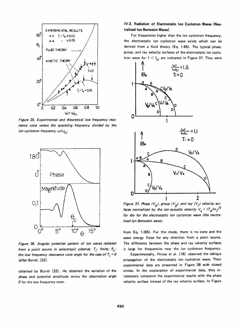
experimental results are in accord with the ray velocitysurface and do not agree with the phase velocity surface.When one refers to the low frequency resonance cone,the angle of which is given by Eq. 1-(70), the cone angleOCc corresponds to the edge angle of the group velcoitysurface of Figure 30. In Figure 35, the experimental lowfrequency cone-angles are indicated with the theoreticalcone angles from the fluid and kinetic theories. When theeffect of the ion temperature T. is included, the cone angleis found to become narrower than that of T1 = 0. The experi-mental results are in agreement with the theoretical cones

which include a finite ion temperature. This fact agrees withthe numerical potential pattern of Figure 36 which was

489

&*- (y.

Vr/ CS

Vp/Cs

10

Po C0TI/ Te 0.0

I11 --A -11 11 A X-

sH

.nrp

O Q2 Oh Q.6 0.8 1.0(/ wcg

Figure 35. Experimental and theoretical low frequency reso-

nance cone versus the operating frequency divided by the

ion cyclotron frequency W/ci.

0 5°I +,5Q 50 1 o0e 150

Figure 36. Angular potential pattern of ion waves radiated

from a point source in anisotropic plasmas. Ti: finite; 69:the low frequency resonance cone angle for the case of T1 = 0

(after Burrel, [221.

obtained by Burrel [22]. He obtained the variation of the

phase and potential amplitude versus the observation angle0 for the low frequency cone.

IV-2. Radiation of Electrostatic Ion Cyclotron Waves (Neu-tralized Ion Bernstein Waves)

For frequencies higher than the ion cyclotron frequency,

the electrostatic ion cyclotron wave exists which can be

derived from a fluid theory (Eq. 1-65). The typical phase,

group, and ray velocity surfaces of the electrostatic ion cyclo-

tron wave for f < fci are indicated in Figure 37. They were

IB1 Ti-OtBo ~ .

I

I

1 2Figure 37. Phase (Vp), group (V,g) and ray (Vr) velocity sur-

faces normalized by the ion acoustic velocity Vs = (Telmi)for the for the electrostatic ion cyclotron wave (the neutra-

lized ion Bernstein wave).

from Eq. 1-(65). For this mode, there is no cone and the

wave energy flows for any direction from a point source.

The difference between the phase and ray velocity surfaces

is large for frequencies near the ion cyclotron frequency.Experimentally, Hirose et al. [181 observed the oblique

propagation of the electrostatic ion cyclotron wave. Their

experimental data are presented in Figure 38 with closed

circles. In the explanation of experimental data, they er-

roneously compared the experimental results with the phasevelocity surface instead of the ray velocity surface. In Figure

490

ex; =1.2Tel Ti=16

VP I Vs

0

89.9995

.0892.9997

0- 89.9999

,/Vs-41

1 25 rVt/VA

o°tI IN

5

Arco/wc =1.2

Ti/Te =0.1

)Jen-in =0

a I I -I

r'¶WVj

1 5+/V;

Figure 38. Experimental ray velocity surface (0) of the electro-static ion cyclotron wave with t7e theoretical ray, phase, andgroup velcoity surfaces. The experimental data are fromHiroseetal. [18].

38, the theoretical phase, group, and ray velocity surfaces

are also indicated, which were obtained from Eq. 1-(65)for their experimental conditions. It may be concluded thattheir experimental results agree with the rayvelocitysurface[23].

Figure 39. Phase (VP), group (Vg), and ray (Vr) velocitysurfaces normalized by the ion thermal velocity Vi = (2T/mi) Y2 for the pure ion Bernstein wave.

hybrid frequency in a warm magnetized plasma has beeninvestigated in detail by Ohnuma et al. [17]. The quasi-statickinetic dielectric constant includes collisions with a rook'smodel. A graph of the phase velocity near the lower hybridfrequency versus the propagation angle d is indicated inFigure 40. The phase velocity is normalized by the ion thermal

IV-3. Radiation of Pure Ion Bernstein WavesTypical phase, group, and ray velocity surfaces for the

pure ion Bernstein wave are shown in Figure 39. They were

obtained from the kinetic dispersion relation (Eq. 11) andEq3. 1-(5)(7)(15). The ray velocity surface is nearly parallelto the magnetic field. The wave fronts of the pure ion Bern-stein wave radiated from a point source are parallel to themagnetic field and the wave normal for all observation pointsare perpendicular to the field lines. In words, cylindrical pureion Bernstein waves can be radiated from a point oscillatingsource.

Although Schmidt observed thi; pure ion Bernsteinwave by using a long line source [24], the radiation pheno-mena from a point source has not been investigated experi-mentally. This mode is very similar to lower hybrid wavesbecause the ray velocity surfaces for both modes are verysimilar to each other. The experiments on the lower hybridmode will be explained in the next section IV-4.

IV4. Radiation of Lower Hybrid WavesRadiation of quasi- tatic plasma waves near the lower

10'

V

10

T / Te =0.1tp /(4,=400C /Ge4=1n05

)),n 4e

i - l. -V.. -~ 4'

1

LowerHybridWave

0 \0.010.05

..x

,'/

Ion Acoustic Wave

0

°° 3e)° 60° 1,89.85X89.85°

Figure 40. Phase velocity (VP) of electrostatic waves near

the lower hybrid frequency versus the propagation angle

dJ The abscissa is stretched near d= 90°.

491

2ljto

I

0

090

2

.5

velocity V. = (2Ti/m.) /2. The angle near the 900 is stretchedin order to clarify the behavior of the velocity. The figureindicates interesting facts that the ion wave and the lowerhybrid wave can propagate for the direction of 0 < d <89.90 and -89.9° < 6 < 900, respectively and that the lowerhybrid wave easily becomes the ion wave with weak colli-sions. The corresponding group and ray velocity surfacesare shown in Figure 41 for both the ion and lower hybrid

8

4

IAW =

0z 89.9999°00

Ar

Opi/ (ci = 400(U/ W>L = 1.05

Ti / Te =0.1

))en/ ce

600

(Ai

400

00

I Vi/ VjI V,r

1z 89.9990°1

I O4 w 89.9995

I "EI,

I

Vg/Vj=VrVI vg/vj

r/V, 0

Ar

T, / Te =0.1I

Exp

/I,I ell(ce=~o'l --41

)er imental

U-X /WC,= 430

4H,=230

K, p, = 105, =710'

100 200

I b90

8 4

Exper mental.. 2

/ Te 0.1

(A/u)/LAc 430

Yen tce C

)/WLI=1 3

Ar

v,/v;

2

[onAcoustic

Wave

Figure 41. Group (Vg) and ray (V,J velocity surfaces of the

lower hybrid wave and the ion wave near the lower hybridfrequency. The corresponding phase velocity is in Figure 40

with Pen =

waves. The angle 6 on those velocity surfaces are the cor-

responding propagation angle on a phase velocity surface.

These velocity surfaces indicate that the ion waves and lower

hybrid waves radiated from a point source have sphericaland cylindrical wave fronts, respectively. Furthermore,they are found to coexist for almost all directions with respectto the point source.

In experiments, the dispersion curve and the ray velocitysurface of the lower hybrid mode are observed for low elec-

tron neutral collisions as shown in Figures 42 and 43, respec-tively. The solid curves are the corresponding dispersioncurve and ray velocity surface from kinetic theory. The

lower hybrid wave is experimentally confirmed to propagate

Figure 43. Experimental and theoretical ray velocity surfacesof the lower hybrid wave.

Exper meqta,* 0

w)p,vu) -.30

;), /~ e 1- ^ 1G-

ck) / A)L w - 3

Ar

904

L Dwer

Hy br C

Wave

6

Figure 44. Experimental and theoretical ray velocity surfacesof the ion acoustic wave near the lower hybrid frequency.

492

K, 1

Figure 42. Experimental dispersion curve of the lower hybridwave in a warm anisotropic,plasnia for Pen/C 10 3.Solid curves are the theoretical ones.

90°4 6

Lower

HybroWave

, , , . .I .%.,%O_ , . --II

T

N0°

IIIIIIIIII

-0

Bo006 i

with cylindrical wave fronts. For a higher pressure withincreased collisions, the ray velocity surface of the ion acousticwave is observed as shown in Figure 44. From this experi-mental results, the ion wave is confirmed to exist near thelower hybrid frequency and is radiated from a point sourcewith spherical wave fronts.

V. RADIATION OF ELECTROMAGNETIC ELECTRONWAVES IN AN ANISOTROPIC PLASMA

Many essential properties of electromagnetic waves inplasmas are included in cold plasmas. The dispersion relationin the cold plasma with ion effects is given as follows:

2 22 P(n -R) (n -L) (12)tan = 2 2

(Sn -RL)(n -P)

n=ck/c, P=1 -c /2 2A 2 /12 2pe pi

R=1 - pe

W2 )JWce

W2i o±c

u 2 Co +Uici

x

(u -UPPERU / H~~YBRID

pe X/

WI X LOWER

~~HYBRID

ALFVEN WAVE K.LFigure 46. Schematical dispersion curves ot electromagneticplasma waves propagating perpendicular to the magneticfield in a cold anisotropic plasma.

of electromagnetic modes in an anisotropic plasma are includ-ed in Figures 45 and 46, although the finite temperatureeffects are not included.

(We (x 2i (1L=1-- -

p

(j2J+Wce W2 (LJ-UciS=(R+L)/2

The schematical dispersion curves in the cold plasma are indi-cated in Figures 45 and 46 for the propagation parallel and

U)

r

WIwce

)ci

R /

L/ELECTRONCYCLOTRON WAVE

-

R /WHISTLER W.

ON CYCLOTRON W.

ALFVEN WAVE K1l

Figure 45. Schematical dispersion curves of electromagneticplasma waves propagating parallel to the magnetic field in acold anisotropic plasma.

perpendicular to the magnetic field. The fundamental modes

V-1. Radiation of Whistler and Electron Cyclotron WavesA simple dispersion relation of whistler and electron

cyclotron waves (right-handed polarized waves) is given by[25]

c2k2c k2 = 1 - 1- (w /c)cos (13)ce

From this relation, phase, group, and ray velocity surfacesare calculated for typical cases of f/fce t 0.5 as shown inFigure 47.

Stenzel has recently observed [11] wave fronts of thesewhistler and electron cyclotron waves. The experimentalresults are shown for two cases of f/fce = 0.8 (the electroncyclotron mode) and 0.285 (the whistler mode) in Figures48 and 49. The typical parameter values were fce ; 235 MHzand fpe/fce t 16.8 and 15.2. Clear wave fronts of electro-magnetic waves are indicated. In Figure 49, the spatial vari-ation of the amplitude of the radiated wave is also indicated.From the experimental wave fronts, the ray velocity surfaceversus the observation angle can be easily obtained in the farfield region. Such ray velocity surfaces from the experimentaldata are plotted in Figures 50 and 51 [26]. The solid curvesare the theoretical ray velocity surfaces which were obtainedaccording to the experimental conditions with use of Eq. 13.For the electron cyclotron wave (Figure 50), the theoreticalray velocity surface is in rough agreement with the experi-

493

lBo'

f Ia -

fce 5 E

f -2- - X10fPe 5

-V9 / c

/c

/C

(xbO )

4 2 0 2 4

L. _/

/ (p

-0-

Figure 48. Experimental wave fronts of the electron cyclotronwave, f/fc >0.5[11].

ce

Bo f 3fca 4

B f 3 -2C - X40c f pe 4

I-

I-0

-

0:KID

Vp / C

-2 c-

W ~~~~(xlO )0.4 0.2 0 02 0.4 Ff

Figure 47. Phase (VP), group (Vg), and ray (Vr) velocity sur--

faces of electromagnetic electron waves, namely, the whistler,wave for flfce < 0.5 and the electron cyclotron wave for

ffce > 0. 5. c: the light velocity.

II

-10 MAX MINIL I

AXIAL POSITION z ICMA)

mental one. For the whistler mode (Figure 51), only one part

of the theoretical ray surface agrees with the experimentalresults in the far field. From these considerations, it may be

concluded that the wave fronts observed by Stenzel can be

explained by a concept of the ray velocity surface.Next, the relation of the whistler wave and the potential

around a launcher detected by Ohnuma is presented. Thedetailed experimental setup will be explained in the followingsections V-2, 3. A magnetic probe 2 cm in diameter and a

monopole 3 mm in length are used as a launcher and a detec-tor, respectively. For a high density plasma (No0 8 x 1010cm3 ), the typical spatial variation of the detected fieldaround the magnetic probe is indicated in Figure 52. The

Figure 49. Experimental wave fronts and amplitude patternsof the whistler wave, flf < 0.5 911].

variation of the peak field is shown. Such a peak potentialas Figure 52 is plotted with closed circles in Figures 53 and54 for two experimental conditions. The theoretical wave

fronts from Eq. 13 and the resonance cone angle for the

experimental conditions are plotted with solid lines. As for

the wave fronts, only two equivalent phase surfaces are indi-

cated in Figures 53 and 54. The experimental results indi-

cated with dotted lines are found to be narrower than thetheoretical ones for both cases. The difference between this

experimental result and Stenzel's result exists for f/fce < 0.5.

494

Vr/C 0.02

0.02

0

60ff8

& 0 /fe~

0.'Id'al 25

f--=0.8fcefpe -16.8fce

0 002

'46

41004

Figure 50. Experimental and theoretical ray velocity surfacesof electron cyclotron wave. The experimental results (@) arefrom the data of Figure 48. 30

0

Vr/C

0

.550

f'°k =0.285

f = 15.2fce

002Figure 51. Experimental and theoretical ray velocity surfacesof the whistler wave. The experimental results are fromFigure 49 in the far field region.

2cm0 Magnetic LoopFigure 52. Field intensity patterns of the whistler wave radiat-ed from a magnetic probe, which is located at Z = 0 cm.

pe ce f =072

Z(cm)\' \' \*, /

30 20 10 0 10 20 3iMagnetic LoonFigure 53. Experimental (") and theoretical (solid lines)

wave fronts of the electron cyclotron wave radiated from amagnetic probe. The experimental data are obtained fromsuch peak positions as Figure 52.

495

0.04I

At

f / e=0.39.A0nnZ

00BoMHZtp2.80omHz

A.450M425 MHz

400 MHz

3715 MHz).uz

L350 MHz/

325 MH:

300 MHz

2715 MH:

20 10 0 10 20R(cm)

Magnetic Loop

Figure 54. Experimental and theoretical (solid curves) wave

fronts of the whistler wave radiated from a magnetic loop.

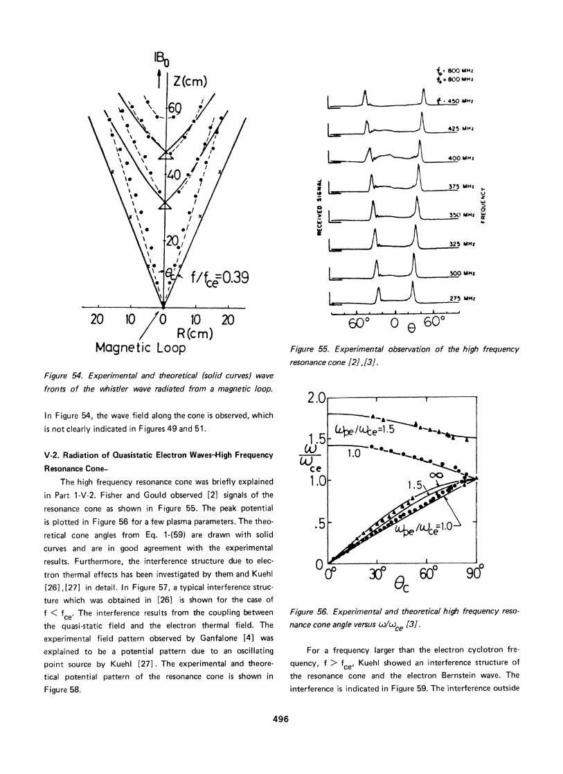
In Figure 54, the wave field along the cone is observed, which

is not clearly indicated in Figures 49 and 51.

V-2. Radiation of Quasistatic Electron Waves-High Frequency

Resonance Cone-

The high frequency resonance cone was briefly explained

in Part 1-V-2. Fisher and Gould observed [2] signals of the

resonance cone as shown in Figure 55. The peak potential

is plotted in Figure 56 for a few plasma parameters. The theo-

retical cone angles from Eq. 1-(59) are drawn with solid

curves and are in good agreement with the experimental

results. Furthermore, the interference structure due to elec-

tron thermal effects has been investigated by them and Kuehl

[26],[27] in detail. In Figure 57, a typical interference struc-

ture which was obtained in [26] is shown for the case of

f < fce. The interference results from the coupling between

the quasi-static field and the electron thermal field. The

experimental field pattern observed by Ganfalone [4] was

explained to be a potential pattern due to an oscillating

point source by Kuehl [27]. The experimental and theore-

tical potential pattern of the resonance cone is shown in

Figure 58.

6 0 o 60Figure 55. Experimental observation of

resonance cone [2],[3].the high frequency

90'

Figure 56. Experimental and theoretical high frequency reso-

nance cone angle versus w/wce [3]

For a frequency larger than the electron cyclotron fre-

quency, f > fce, Kuehl showed an interference structure of

the resonance cone and the electron Bernstein wave. The

interference is indicated in Figure 59. The interference outside

496

IB

a

WIa

030

the cone angle Oc results from the coupling between the

8 , . quasistatic field and the electron Bernstein wave. The quasi-static field which is used here is the field which can exist in

,/1 | a cold plasma. Gonfalone et al. observed [51 the potentialpatterns radiated from a small probe for frequencies both

-4L 0 higher and lower than the electron cyclotron frequency(Figure 60) and explained quantitatively, the potential pat-

*,: A tA s X S | terns as being due to a coupling to the electron Bernsteinwave. This explanation for the experimental potential pattern(Figure 60d) is shown in Figure 60.

400 600 e go°

Figure 57. Angular potential pattern near the resonance cone

in a warm anisotropic electron plasma, f/f = 0.6, f/f =0.95. and rfrL =500 [26]. c pe A1d

'~~~\l3

0a

L&J

00 300 6 d0dFigure 58. Experimental and theoretical potential patternof oscillating point source, f/f 0.54, f/f = 0.64, and Yece pe e

r/rL = 200 [27]. W- WV\

100 go9 '600 300 I0 300 60 goo

Figure 60. Experimental potential resonance cone above3'.- F11 1 Iand below the electron cyclotron frequency with the theo-

retical pattern (e) for the corresponding datum (d) [5].

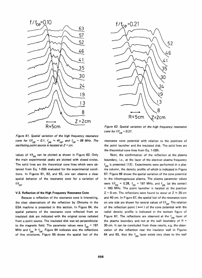
50 - In Figures 61 and 62, the spatial variation of the reso-nance cone radiated from a point source is clearly indicatedfor the case of f/fce = 0.1 and 0.21, where fce = 98 MHz,and f 4fce The launcher is located at Z = 0 cm. Thepe cdirections parallel and perpendicular to the magnetic fieldare Z and R respectively. The value of Z is the distance from

030 60 90° the point source to the observation point along the magnetic900 60field. These experimental results were recently detected

Figure 59. Angular potential pattern of the electron Bernstein in the ESA-ESTEC machine by Ohnuma. The propagation ofwave with the resonance cone field, f/f = 1.7, f/f = 1.21, the fine structure is also indicated. From such experimentala10ce peand r/rL =500 [26]. data, the spatial variation of the resonance cone for several

497

f /fro=0.21

52

Figure 62. Spatial variation of the high frequency resonance

cone for flfe = 0.21.Figure 61. Spatial variation of the high frequency resonance

cone for f/fe ,01 f - 4fce and foe = 98 MHz. Thecon fo llce pe

oscillating point source is located at Z = cm.

values of f/fce can be plotted as shown in Figure 63. Onlythe main experimental peaks are plotted with closed circles.The solid lines are the theoretical cone lines which were ob-

tained from Eq. 1-(59) evaluated for the experimental condi-tions. In Figures 61, 62, and 63, one can observe a clear

spatial behavior of the resonance cone for a variation of

f/fce

V-3. Reflection of the High Frequency Resonance Cone

Because a reflection of the resonance cone is interesting,

the clear observations of the reflection by Ohnuma in the

ESA machine is presented in this section. In Figure 64, thespatial patterns of the resonance cone reflected from an

insulated disk are indicated with the original cones radiatedfrom a point source. The insulated disk was set perpendicularto the magnetic field. The parameter values were fce = 197

MHz and f > fce Figure 64 indicates also the reflectionspe ces

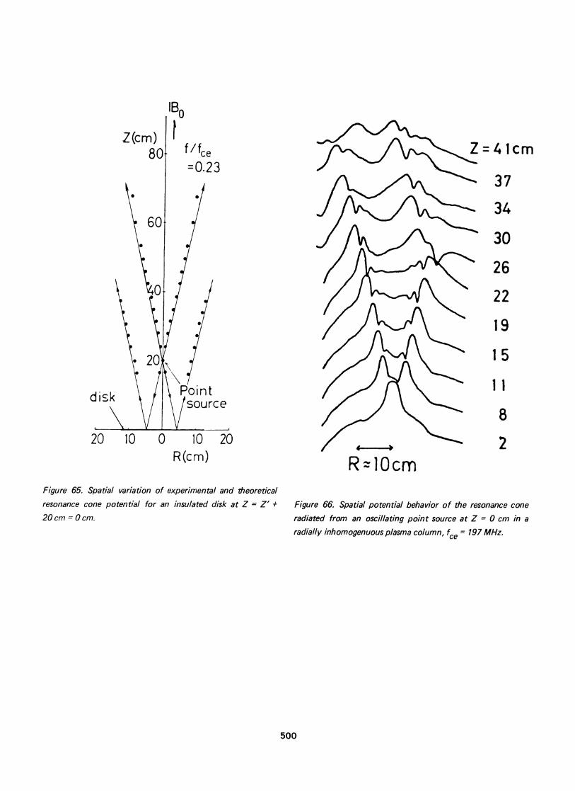
of fine structures. Figure 65 shows the spatial loci of the

resonance cone potential with relation to the positions of

the point launcher and the insulated disk. The solid lines are

the theoretical cone lines from Eq. 1-(59).Next, the confirmation of the reflection at the plasma

boundary, i.e., at the layer of the electron plasma frequency

fpe is presented [131. Experiments were performed in a plas-

ma column, the density profile of which is indicated in Figure67. Figure 66 shows the spatial variation of the cone potentialin the inhomogenuous plasma. The plasma parameter valueswere f/fce = 0.28, fe = 197 MHz, and fpe (at the center)= 160 MHz. The point launcher is located at the positionZ = 0 cm. The reflections were found to occur at Z t 25 cmand 40 cm. In Figure 67, the spatial loci of the resonance cone

on one side are shown for several values of f/fce The relationof the reflection point ( ~-4 ) of the cone potential with the

radial density profile is indicated in the bottom figure of

Figure 67. The reflections are observed at the fpe layer ofthe plasma boundary and not at the wall boundary of R =

30 cm. It can be concluded from these results, e.g. the obser-vation of the reflection near the insulator wall in Figures64 and 65, that the fpe layer exists very close to the wall

498

R - 5cm

10 20R(cm)

Point source

Figure 63. Experimental and theoretical (solid lines) spatialvariation of the high frequency resonance cone for variousff 4f .fce pe ce'

fnfce0.233

/L 30f / fce=0.06

a

o 0.210

0

a

XO 0.410

0x

0x

Oi 0.77f--4 cm

R.Ocm

Figure 64. Spatial variation of the resonance cone with aninsulated disk at Z' = -20 cm. The oscillating point sourceis located at Z'= 0 cm. f > f = 197 MHz.pe ce

499

IBOz(cm) l

20

IBO

Z(cm)80

d isk

20

f/fce=0.23

=41cm

37

34

30

26

22

19

15

1 1)int

R(cm)

Figure 65. Spatial variation of experimental and theoreticalresonance cone potential for an insulated disk at Z = Z' +

20 cm = 0 cm.

8

24R-Oc

R-lOcm

Figure 66. Spatial potential behavior of the resonance coneradiated from an oscillating point source at Z = 0 cm in aradially inhomogenuous plasma column, fce = 197 MHz.

500

f / fce= 0.1 5- °

60\

0.23- .

40

0.38-

20-

20 10

F2 4Fr

3

the duct propagation of rf-field in the higher density region.

10 20R (cm)

No

30 20 10 0 10 20 30R(cm)

Figure 67. Experimental and theoretical loci of the resonance

cone (top figure) in an inhomogenuous plasma column, thedensity profile of which is given in the bottom figure. Thesymbols (1-) in the bottom figure are the experimentalreflection points.

in the experiments. In other words, one can observe the fpelayer by using the measurement of the reflection of theresonance cone. Furthermore, Fkjures 66 and 67 indicate

VI. RADIATION OF ELECTROMAGNETIC IONWAVES IN AN ANISOTROPIC PLASMA

A simple dispersion relation of the electromagnetic ionwaves, namely, the hydromagnetic mode, is given byW =rkVAcosy (torsional) (14)

k [A sLAs As±)

2V V2 c o s2 1/2 }/2 1/ (15)

A s (compress sional)

Typical phase, group, and ray velocity surfaces for the tor-sional and compressional Alfven waves are indicated in Figures68 and 69. Those velocity surfaces for Alfven waves have not

IB0 A.B,C

V9 /VA /

Vr /VA

0.5 vP/VA

0.5 0 0a5 1

Figure 68. Phase (Va), group (Vg). and ray (V.) velocity sur-

faces for electromagnetic ion waves, i.e., torsional Alfvenwaves. VA: the Alfven velocity and VS: the ion acousticvelocity.

been observed experimentally up to the present becauseof the difficulty of producing the appropriate plasma.

VII. RADIATION IN A PLASMA STREAM

The radiation phenomena in a stable system with astream is presented in this section as an example of the stream-ing effects, although unstable systems with a stream have beeninvestigated in [12] and [161. In particular, radiation of anion acoustic wave in a plasma stream with velocity IV, is

501

A typical phase velocity surface which was obtained from

Eq. 17 is indicated in Figure 70, in which U is the normalized

VS /VA =1.1

0:o

4

U

I 0 1 2 Figure 70. Phase velocity surfaces of ion acoustic waves ina plasma stream. U = Vo/Vs, VO: the stream velocity and

4. ,I,, -I VS the ion acoustic velocity.VA /'S : I.'

Vp / Vs

velocity of U = VO/V . The group velocity surface from Eq.

17 is shown in Figure 71. In this case, the ray velocity surface

2'

0:0O I 1:1 U=2 0:3 UtT4

-2

I 0 1 1 2(V2 V)1/2VA Vs

Figure 69. Phase (VP), group (Vg), and ray (V,) velocity sur-

faces for electromagnetic ion waves, i.e., compressional Alfven

waves. VA: the Alfven velocity and Vs: the ion acoustic

velocity.

described here. Using fluid equations the dispersion relation

is derived.

2 W piD(W,lk) = k{1 - pI

(W -lk-\Vo)2-k2Ci

(U. - Ik.Wo) 2 -k2C2} (16)

For k2CC2 << l1 - Ik.1V 12 < k2Ce2 and k2 < k e2 this equa-

tion becomes 2 uA)2.khe ( p1 0 (17)

k ~e (u.j- lk.\VO)2

-21Figure 71. Group (= ray) velocity surfaces of ion acoustic

waves in a plasma stream, U = VO/VS.

is in agreement with the group velocity surface. Figure 71

shows that the energy flow of the ion acoustic wave radiated

from a point source is more localized with an increase of the

velocity. As shown in Figures 70 and 71, there exists two

modes in the plasma stream, namely, the slow and fast modes

[281. Figure 71 shows typical phase, group, and ray velocity

surfaces for a half space. The relation between these velocity

surfaces is indicated in Figure 72. When one uses Eq. 16 and

considers the anisotropy of the temperature, Figure 72 be-

comes Figure 73. Those velocity surfaces are shown in Figure

74 for all directions in detail. The frequency is normalized as

Q = w/cop. The relation between the slow and the fast

modes is clearly noted.Finally, preliminary experimental results on the group

velocity surfaces are indicated in Figure 75 with closed circles.

The experimental results were obtained using pulse propa-

502

I 2IB1

vsVA

V9/VAvr /VA'1

Vp /VA

12180

VA-Vs -

Vg/Vs

Vr /Vs

II

UJ=2

,VP

-2 -1 O i\ 2-1 Vg. Vr

u

Figure 72. Relation of phase, group, and ray velocity surfacesof ion acoustic waves in a plasma stream (from Eq. 17).

3.Figure 74. Phase (Va), group (Vg). and ray (V,) velocitysurfaces of fast and slow ion waves in a plasma stream.

2

-2 -1

-i

0906r

Flow_ ,-2 3 4 5

U =3.741

21

Figure 73. Phase, group, and ray velocity surfaces of ion waves

in a plasma stream (from the modified Eq. 16).

gation in a plasma stream. Because there existed rest ionsdue to charge exchange [29], the ion mode radiated from th

point source is also observed. The corresponding theoreticalgroup velocity surface is shown with solid curves.

REFERENCES

Exciter

Ion Mode

- J

2 4.70To

Theory

Figure 75. Experimental and theoretical group velocity sur-

faces of ion waves in a plasma stream with rest ions.

1 W.P. Allis, et al., Waves in Anisotropic Plasmas, MIT

Press, 1963.2 R.K. Fisher and R.W. Gould, Phys. Rev. Let. 22, 1093

(1969).3 R.K. Fisher and R.W. Gould, Phys. Fluids 14, 857 (1971).4 A. Gonfalone, J. Phys. 33, 521 (1972).5 A. Gonfalone and C. Beghin, Phys. Rev. Let. 31, 866

(1973).6 D.B. Muldrew and A. Gonfalone, Rad. Sci. 9, 1159

(1974).7 T. Ohnuma et al., submitted to J. Phys. Soc. Jpn.

8

9

1011

1213

14

1516

R.W. Boswell, Nature 258, 58 (1975).R.W. Boswell and M.J. Giles, Phys. Rev. Let. 36, 1142

(1976).M.D. Simonutti, Phys. Fluids 19, 608 (1976).R.L. Stenzel, Phys. Fluids 19, 857 (1976).R.L. Stenzel, Phys. Rev. Let. 38, 394 (1977).T. Ohnuma and B. Lembege, submitted to Phys. Fluids.

S. Ohmori et al., Rad. Sci. 11, 531 (1976), and submit-ted to Rad. Sci.T. Ohnuma et al., Phys. Rev. A 12, 1648 (1975).T. Ohnuma et al., Phys. Rev. Let. 36, 471 (1976).

503

3 4

a Fast Mode0

I

6 8-;U

x -~~~~~~~~~~~~~~~~~~~~~~~~~~~~~~~~IlA

17 T. Ohnuma et al., Phys. Rev. A 16, 387 (1977).18 A. Hirose et al., Phys. Fluids 13, 1290, 2039 (1970).19 T. Ohnuma et al., Phys. Rev. Let. 37, 206 (1976).20 T. Ohnuma et al., Phys. Rev. A 15, 392 (1977).21 P. Belan, Phys. Rev. Let. 37, 903 (1976).22 K.H. Burrel, Phys. Fluids 18, 897 (1975).23 T. Ohnuma, Kakuyugo Kenkyu 38, 159 (1977) (cir-

cular in Japanese).24 J.P.M. Schmidt, Phys. Rev. Let. 31, 982 (1973).25 R.A. Helliwell, Whistlers and Related Ionospheric Phe-

nomena, Stanford Univ. Press, 1965.26 H.H. Kuehl, Phys. Fluids 16, 1311 (1973).

27 H.H. Kuehl,Phys. Fluids 17, 1275 (1974).28 T. Ohnuma and Y. Hatta, J. Phys. Soc. Jpn. 33, 907

(1967).29 T. Ohnuma and T. Fujita, Phys. Fluids 16, 2026 (1973).

FURTHER REFERENCES

1 T.H. Stix, The Theory of Plasma Waves, McGraw-Hill,1962.

2 T. Ohnuma, Kakuyugo Kenkyu 38, 303 (1977) (circularin Japanese).

504