Radiation Exchange Between Surfaces - Auburn Universitydmckwski/mech7210/radexchan… · · 2007-03-15Radiation Exchange Between Surfaces 1.1 Motivation and Objectives Thermal radiation,

Chapter 1

Radiation Exchange Between Surfaces

1.1 Motivation and Objectives

Thermal radiation, as you know, constitutes one of the three basic modes (or mechanisms) of heattransfer, i.e., conduction, convection, and radiation. Actually, on a physical basis, there are onlytwo mechanisms of heat transfer; diffusion (the transfer of heat via molecular interactions) andradiation (the transfer of heat via photons/electomagnetic waves). Convection, being the bulktransport of a fluid, is not precisely a heat transfer mechanism.

The physics of radiation transport are distinctly different than diffusion transport. The latteris a local phenomena, meaning that the rate of diffusion heat transfer, at a point in space, preciselydepends only on the local nature about the point, i.e., the temperature gradient and thermalconductivity at the point. Of course, the temperature field will depend on the boundary and initialconditions imposed on the system. However, the diffusion heat flux at, say, one point in the systemdoes not directly effect the diffusion flux at some distant point. Radiation, on the other hand, isnot local; the flux of radiation at a point will, in general, be directly and instantaneously dependenton the radiation flux at all points in a system. Unlike diffusion, radiation can act over a distance.Accordingly, the mathematical description of radiation transport will employ an integral equationfor the radiation field, as opposed to the differential equation for heat diffusion.

Our objectives in studying radiation in the short amount of time left in the course will be to

1. Develop a basic physical understanding of electromagnetic radiation, with emphasis on theproperties of radiation that are relevant to heat transfer.

2. Describe radiation exchange among surfaces, in which the surfaces can be perfect absorbersof radiation (black) or diffusely absorbing (gray).

3. Introduce the topic of radiation transfer in a participating medium that absorbs, emits, andscatters radiation, and describe the formulation and application of the radiative transportequation.

1

2 CHAPTER 1. RADIATION EXCHANGE BETWEEN SURFACES

1.2 Basic Radiation Properties

For our purposes, it is useful to view radiation as the transport of energy in electromagneticwaves. Radiation can also be viewed as the transport of energy by discrete photons, and the basicrelationship between the energy of a photon, ǫ, and the frequency ν or wavelength λ = c/ν of thewave is given by Planck’s relation;

ǫ = h ν =hc

λ(1.1)

where h is Planck’s constant and c is the speed of light in a vacuum.Equation (1.1) indicates that the energy of the radiation is inversely proportional to the radiation

wavelength. Thermal radiation refers to the spectrum of radiation in the visible (λ = 0.4−0.7 µm)to infrared (IR, λ = 0.7 ∼ 10 − 100 µm) wavelengths. Radiation at these wavelengths can excitethe rotational and vibrational energy levels of molecules and thus transfer energy to molecules inthe form of heat. That is, the absorption of thermal radiation by molecules will act to raise thetemperature of the system. Radiation having shorter wavelengths (UV, x–rays, γ–rays) can excitethe electronic energy levels of molecules and atoms and/or ionize or break molecular bonds. Thisspectra of radiation is often referred to as ionizing radiation. On the other hand, longer wavelengths(microwaves, radio waves) will not, in general, couple with the energy storage levels in molecules;although an obvious exception are the microwave wavelengths used in the common microwave oven.

In practically all engineering–relevant applications, the source of thermal radiation is thermal

emission. All bodies at any finite temperature will emit radiation. It was theoretically establishedby Boltzmann, and experimentally confirmed by Stephan, in the 19th century that the maximumpossible emission rate from a surface is given by

eb = σT 4 (1.2)

where σ = 5.67× 108 W/m2 K4. The above formula is known as the Stephan–Boltzmann law, andeb, having units of W/m2, is the blackbody emissive power, which depends solely on the absolutetemperature T of the surface. All real surfaces will emit radiation at a rate smaller than eb; an‘ideal’ surface which attained an emission of eb would be referred to as a blackbody.

It is possible to construct devices which come very close to meeting the ideal emission of ablackbody. Typically, these devices are formed from an isothermal cavity (i.e., a hollow sphere),with a small opening from which the radiation escapes. The radiation emitted by a blackbody ata specified T will be distributed over wavelength λ, the spectrum of which will also depend solelyon T . Although the nature of the blackbody spectrum was experimentally known in the late 19thcentury, theoretical prediction of the spectrum defied the ‘classical’ physical understanding of theday. Planck, at the beginning of the 20th century, used the concept of discrete wavelength energylevels to develop a theoretical prediction of the blackbody spectrum which was consistent withexperiments. His formula for the spectral blackbody emissive power is

ebλ =C1

λ5 (exp[C2/(λT )] − 1)(1.3)

1.2. BASIC RADIATION PROPERTIES 3

10−1

100

101

102

10−3

10−2

10−1

100

101

102

103

104

105

106

λ, µ m

e bλ, W

/m2 µ

m

1000 K1500 K2000 K

Figure 1.1: Blackbody spectral power distribution

in which C1 = 2πhc2 = 3.7413 × 108 W (µm)4/m2 and C2 = hc/kB = 14, 388 µm K. The quantityebλdλ denotes the energy emitted from the black surface, per unit area, within a wavelength intervaldλ about wavelength λ. The energy over all wavelengths is obtained from

eb =

∫

∞

0ebλ dλ = σ T 4 (1.4)

i.e., the total emissive power is given by the Stephan–Boltzmann law, as it must.A plot of ebλ vs. wavelength λ is given in Fig. 1.1. As T increases two things happen: 1) the

spectral emissive power at all wavelengths increase, and 2) the wavelength corresponding to themaximum power shifts towards the shorter wavelengths. The value of the wavelength at which themaximum occurs is predicted by the Wien displacement law,

λmax =2898 µm K

T(1.5)

Equation (1.4) can be rearranged to identify a fractional distirbution function. Assume that Tis constant, then we can write

1

σT 5

∫

∞

0ebλ d(λ T ) = 1 (1.6)

Now combine with Eq. (1.3), and observe that λT becomes the sole variable of the distribution.We can therefore define

f ′(λT ) =C1/σ

(λT )5 (exp[C2/(λT )] − 1)(1.7)


Figure 1.2: Intensity definition

so that

f(λT ) =

∫ λT

0f ′(x) dx (1.8)

represents the fraction of emitted energy between 0 and λT , relative to the total emitted energy.

Intensity

The previous section identified the blackbody emissive power from a surface, which is a quantitythat has units of W/m2, that is, the same units of a heat flux. The emissive power, however, isnot a heat flux – the latter is precisely a vector quantity which can be resolved into directionalcomponents. The emissive power, on the other hand, describes the energy leaving a surface perunit area of the surface; it does not describe the directional characteristics of the radiation as itleaves the surface.

To describe the directional properties of radiation as it propagates through space, we need tointroduce a quantity referred to as the radiation intensity. The intensity, denoted I, is defined byuse of Fig. 1.2. Radiation is emitted from a small surface element ∆A and travels in all directions.A portion of the radiation lands on the small area element on a hemisphere enclosing ∆A, denotedas dA. With regard to geometrical considerations, it should be easy to see that the net amount ofenergy falling on dA, which is denoted as dP , will be proportional to

1. the projected area of the emitting surface, which would be ∆A cos θ,

2. the area of the ‘target’, dA, and


3. the inverse square of the distance between the source and the target, 1/R2.

The last proportionality comes from the fact that the area of the hemisphere scales as R2, and thetotal power falling on the hemisphere – which would equal the total power emitted by the source– would be constant in the absence of a participating medium. So the power per unit area on thehemisphere would go as 1/R2.

The target area dA can be related to the distance R by the polar coordinates;

dA = R2 sin θ dθ dφ (1.9)

Note that∫

dA = R2

∫ π/2

0sin θ dθ

∫ 2π

0dφ = 2πR2 (1.10)

as expected. Now dP is proportional to dA/R2, and

dA

R2= sin θ dθ dφ ≡ dΩ (1.11)

defines a differential solid angle dΩ. The units of solid angle are the steradian (abbreviated str),and 4π steradians encompass all directions about the origin of a spherical coordinate system.

With our solid angle definition, we now see that the power falling on the target will be pro-portional to the projected area of the source and the solid angle subtended by the target withrespect to the source. The power will also be proportional to the magnitude and directionality ofthe radiation leaving the source and propagating through space. Since dP will be in watts, and dPwill be proportional to ∆A cos θ dΩ, it follows that radiation propagating through space must haveunits of W/m2 str. This quantity is referred to as the intensity, and is defined by

I =dP

∆A cos θ dΩ(1.12)

taken in the limit of ∆A−→0 and dΩ−→0.

The intensity is a difficult quantity to grasp. Although it represents the directional distributionof propagating radiation, the intensity is not a vector in the sense that it cannot be resolved intovector components. Rather, the intensity is a scalar that is dependent on the directional coordinatesθ and φ as well as the usual spacial coordinates and time. In a sense, I is a scalar which is relevantto the 5–D ‘space’ defined by x, y, z and θ, φ.

It was implicitly assumed that the intensity, defined in the Eq. (1.12), represents a wavelength–integrated (or total) quantity. The spectral intensity Iλ is defined by a relation similar to Eq. (1.12),except now on a per–unit–wavelength basis;

Iλ =dPλ

∆A cos θ dΩ dλ(1.13)


where the limit is again taken, and dPλ is the power, in W, falling on the surface dA within thewavelength interval dλ about λ. It follows that

I =

∫

∞

0Iλ dλ (1.14)

Blackbody Intensity

If the surface ∆A is a black surface – meaning that it emits as a perfect blackbody – the intensitydistribution leaving the surface will be independent of direction, i.e., the blackbody intensity Ib

landing on the hemisphere in Fig. 1.2 would not be a function of θ. It is important to note thatthe power per unit area landing on the hemisphere, dP/dA, would be a function of θ; this quantitywould be proportional to the projected area of the source, ∆A cos θ. The intensity, however,represents the power per unit projected area, and so this quantity would remain constant.

The total power leaving the black source would be P = eb ∆A, and in the absence of anintervening medium the total power leaving the source would be the total power landing on thehemisphere. If we use Eq. (1.12), and note that the intensity I = Ib is constant, then

P = eb ∆A

=

∫

dP = Ib ∆A

∫

Ω=4πcos θ dΩ

= Ib ∆A

∫ 2π

0dφ

∫ π/2

0cos θ sin θ dθ

= π Ib ∆A (1.15)

orIb =

eb

π(1.16)

Radiative Heat Flux

As mentioned previously, the intensity, which is a scalar, describes the directional distribution ofradiation energy transfer. The radiative heat flux, qR, is a vector which describes the net directionand magnitude of radiant energy transfer in space.

Say we take a small surface element in space, dA, oriented so that its normal points in thepositive z direction. Radiation, arriving from all directions with an intensity distribution I(θ, φ),passes through the element. The net rate at which energy is transported across the surface, denotedas dP , will be

dP = dA

∫ 2π

φ=0

∫ π

θ=0I(θ, φ) cos θ sin θ dθ dφ

Note that the cos θ term appears because dA cos θ is the projected area of the element with respectto the θ direction. The quantity dP will be either positive, negative, or zero; if it is positive, it


means that the net transfer of energy across dA is in the positive z direction, negative means the netenergy transfer is in the negative z direction, and zero means that there is no net transfer. The lastcondition does not necessarily imply that I = 0; rather, it implies that the positive and negativecontributions cancel out. Such would be the case if the intensity distribution were isotropic, i.e.,independent of direction.

The radiative heat flux, in the z direction, would be dP/dA. The three components of radiativeflux with respect to a cartesian coordinate system are given by

qR,x =

∫ 2π

φ=0

∫ π

θ=0I(θ, φ) sin2 θ cos φdθ dφ (1.17)

qR,y =

∫ 2π

φ=0

∫ π

θ=0I(θ, φ) sin2 θ sinφdθ dφ (1.18)

qR,z =

∫ 2π

φ=0

∫ π

θ=0I(θ, φ) cos θ sin θ dθ dφ (1.19)

1.2.1 Surface Properties

Surfaces can emit, absorb, and reflect radiation. You are certainly familiar with the basic conceptsof surface absorptivity and reflectivity, i.e., the absorptivity α represents the fraction of incidentradiation on a surface that is absorbed by the surface. We will need to develop more precisedefinitions than this to account for the directional and spectral dependencies of the radiationfalling on or emitted by a surface.

Emissivity

As mentioned in the previous section, the intensity emitted by a blackbody is independent ofdirection and given by Ib = eb/π. Likewise, the spectral (or wavelength–dependent) blackbodyintensity is independent of direction and given by Ibλ = ebλ/π. The emitted spectral intensityfrom a real surface, into some direction θ, φ and within a small wavelength interval about λ, willalways be less than the spectral blackbody intensity for a surface at the same temperature. Wecan therefore define the spectral directional emissivity ǫ′λ as

ǫ′λ =Ie,λ(θ, φ)

Ibλ(1.20)

in which Ie,λ is the emitted intensity from the surface; it does not include components due toother sources such as reflected intensity. The spectral directional emissivity represents the mostfundamental, or irreducible, information on the emission properties of a surface. In general, it wouldbe a function of direction, wavelength, temperature, and the physical and chemical properties ofthe surface.


We can obtain averaged emissivity properties by integration of ǫ′λ. The spectral hemispherical

emissivity represents the directional average of ǫ′λ, and is defined by

ǫλ =

∫ 2π

φ=0

∫ π/2

θ=0Ie,λ(θ, φ) cos θ sin θ dθ dφ

∫ 2π

φ=0

∫ π/2

θ=0Ib,λ cos θ sin θ dθ dφ

=

∫ 2π

φ=0

∫ π/2

θ=0ǫ′λ(θ, φ) cos θ sin θ dθ dφ

π

=eλ

eb,λ(1.21)

That is, ǫλ is the ratio of the emitted spectral power from the surface, eλ to the blackbody powereb,λ.

Likewise, the total directional emissivity ǫ′ is obtained from an appropriate wavelength averageof ǫ′λ;

ǫ′ =

∫

∞

0Ie,λ dλ

∫

∞

0Ibλ dλ

=

∫

∞

0ǫ′λ Ib,λ dλ

Ib(1.22)

Finally, the total hemispherical emissivity ǫ is obtained from either a directional average of ǫ′

or a wavelength average of ǫλ; either would yield the same result, which is

ǫ =

∫

∞

λ=0

∫ 2π

φ=0

∫ π/2

θ=0Ie,λ(θ, φ) cos θ sin θ dθ dφ dλ

∫

∞

λ=0

∫ 2π

φ=0

∫ π/2

θ=0Ibλ cos θ sin θ dθ dφ dλ

=

∫ 2π

φ=0

∫ π/2

θ=0ǫ′(θ, φ) cos θ sin θ dθ dφ

π

=

∫

∞

λ=0ǫλ Ibλ dλ

Ibλ

=e

eb(1.23)


Absorptivity

Consider now a surface that is exposed to an incident source of spectral intensity, denoted asI−λ (θ, φ). The – superscript indicates that the radiation is moving downwards onto the surface.When the radiation strikes the surface a fraction of it will be absorbed by the surface, the remainderwill be reflected1. Denote the absorbed intensity as Ia,λ. The spectral directional absorptivity α′

λ isdefined by

α′

λ =Ia,λ

I−λ(1.24)

That is, it is the fraction of incident spectral intensity that was absorbed by the surface.

Similar to the spectral directional emissivity ǫ′λ, the spectral directional absorptivity describesthe fundamental absorption properties of the surface. And as was done with the emissivity, we candefine averages, with respect to direction, wavelength, or both, by appropriate integrations.

The spectral hemispherical absorptivity αλ is

αλ =

∫ 2π

φ=0

∫ π/2

θ=0Ia,λ(θ, φ) cos θ sin θ dθ dφ

∫ 2π

φ=0

∫ π/2

θ=0I−λ (θ, φ) cos θ sin θ dθ dφ

=

∫ 2π

φ=0

∫ π/2

θ=0α′

λ(θ, φ) I−λ (θ, φ) cos θ sin θ dθ dφ

q−λ

=qa,λ

q−λ(1.25)

where q−λ and qa,λ are the downward spectral flux on the surface and the spectral absorbed flux.

The total directional absorptivity α′ is

α′ =

∫

∞

0Ia,λ dλ

∫

∞

0I−λ dλ

=

∫

∞

0α′

λ I−λ dλ

I−(1.26)

1Some of the radiation might also be transmitted through the surface, but at this point we will not make this

distinction; if the radiation is not reflected, then it went into the surface material and was absorbed by it


and the total hemispherical absorptivity α is

α =

∫

∞

λ=0

∫ 2π

φ=0

∫ π/2

θ=0Ia,λ(θ, φ) cos θ sin θ dθ dφ dλ

∫

∞

λ=0

∫ 2π

φ=0

∫ π/2

θ=0I−λ cos θ sin θ dθ dφ dλ

=

∫ 2π

φ=0

∫ π/2

θ=0α′(θ, φ)I− cos θ sin θ dθ dφ

q−

=

∫

∞

λ=0αλ q−λ dλ

q−

=qa

q−(1.27)

All these definitions look analogous to those for the emissivity. An important distinction,though, is in regard to the ‘weighting function’ used to obtain the averages. The blackbody inten-sity Ib is not a function of direction, so it could be removed from the integrals over direction inEq. (1.21) and (1.23) for the hemispherical emissivities. On the other hand, the incident intensityI− (either spectral or total) is, in general, a function of direction, and it cannot be removed fromthe corresponding formulas for hemispherical absorptivity in Eqs. (1.25) and (1.27). This pointsout an important fact: the hemispherical absorptivity will be a function of the directional intensitydistribution falling on a surface. For example, a surface illuminated by the sun from the normaldirection would, in general, have a different hemispherical absorptivity than the same surface il-luminated by the sun at an oblique angle, or by the sun on a cloudy day (diffuse illumination).Likewise, the total absorptivity (either directional or spectral) will be a function of the spectraldistribution of the incident radiation. A surface illuminated by visible light would likely have adifferent total absorptivity than the same surface illuminated by IR radiation.

Reflectivity

Reflectivity is one step more complicated than absorptivity. On the most basic level, the reflectivitywill depend on the angle of the incident radiation as well as the angle of the reflected radiation. Asbefore, denote as I−λ (θ, phi) the incident intensity, and let I+

λ (θ′, φ′) denote the reflected intensityfrom the surface in the direction θ′, φ′. The spectral bidirectional reflectivity ρ′′λ is defined by

ρ′′λ(Ω, Ω′) =I+λ (Ω′)

πI−λ (Ω)(1.28)


The reason for the π in the denominator will become obvious shortly. The spectral directional–

hemispherical reflectivity ρ′λ is obtained by integration of the reflected intensity over the hemisphere;

ρ′λ =

∫ 2π

φ′=0

∫ π/2

θ′=0I+λ (θ′, φ′) cos θ′ sin θ′ dθ′ dφ′

πI−λ (θ, φ)

=1

π

∫ 2π

φ′=0

∫ π/2

θ′=0ρ′′λ(θ, φ, θ′, φ′) cos θ′ sin θ′ dθ′ dφ′ (1.29)

All of the radiation incident on the surface is either absorbed by the surface (again we assumetransmission through the material counts as absorption) or reflected. Consequently,

α′

λ + ρ′λ = 1 (1.30)

Formulas for the hemispherical–hemispherical reflectance are analogous to used for the hemispher-ical absorptivity.

Kirchoff’s Law

Only when one goes to the spectral directional level does the absorptivity become independent ofthe properties (spectral, directional) of the intensity falling on the surface. For a given surface, α′

λ,at a particular direction and wavelength, would not depend upon whether the incident intensity atthis direction and wavelength was produced from, say, a laser or an incandescent source.

The spectral directional absorptivity α′

λ is therefore a function solely of the surface materialproperties – as is the case with ǫ′λ. Indeed, it can be shown from thermodynamic principles thatthe emissivity and absorptivity are equal on the spectral directional level,

α′

λ = ǫ′λ (1.31)

This equality is commonly referred to as Kirchoff’s law.

It is easy to show, using Kirchoff’s law and Eqs. (1.25–1.27), that if the incident intensityarriving at a surface originates from a blackbody that a) completely surrounds the surface, so thatthe incident intensity is independent of direction, and b) is at the same temperature of the surface,so that the incoming intensity has the same spectra as a blackbody emission from the surface, thenemissivity and absorptivity will be equal on the hemispherical and total levels. This condition, i.e.,equal temperatures of source and target, would correspond to thermal equilibrium for which therecould be no net heat transfer between the source and target. In most engineering applications ofrelevance, the incident intensity on a surface will be directionally depend, and will originate froma source that is not at the surface temperature. And for such cases Kirchoff’s law, in general, willnot hold at either the directional or the hemispherical levels.


We can, however, apply approximations to extend the application of Kirchoff’s law. Firstly, asurface with emission and absorption properties that are independent of wavelength will have equalemissivity and absorptivity on the total level. From Eqs. (1.22) and (1.26), it can be seen that ifǫ′λ = ǫ′ 6= func(λ), then ǫ′ = α′. Surfaces with wavelength–independent properties are referred toas gray surfaces.

Likewise, if the spectral directional emissivity is constant for all directions, i.e., ǫ′λ = ǫλ 6=func(theta, φ), then ǫλ = αλ. Surfaces with directionally–independent properties are referred to asdiffuse.

Only for surfaces that are both gray and diffuse can Kirchoff’s law be applied at the totalhemispherical level, i.e.,

ǫ = α, gray, diffuse surfaces (1.32)

The diffuse approximation is relatively accurate for surfaces that have a roughness on thescale of the radiation wavelength or greater, such as oxidized metals, wood, paper etc. Diffuseabsorbers/emitters will also be diffuse reflectors, meaning that the reflection of intensity from asurface is isotropic (independent of direction), regardless of incident direction of the intensity.

The gray approximation is more of a stretch of reality. It is fairly accurate when the sourceof incident radiation is a blackbody at a temperature close to the temperature of the surface ontowhich it is falling; for such cases the spectra of the incident and emitted intensities will be aboutequal.

The gray assumption can fail miserably, however, when the incident radiation has a significantlydifferent spectra than the emitted radiation. A common example is sunlight falling on a solarcollector. The radiation spectrum of sunlight is similar to that of a blackbody at Ts ≈ 5800 K,and is concentrated mainly in the visible wavelengths. Solar collectors, on the other hand, willtypically operate at a temperature of around Tc ≈ 350 K, and emission at this temperature willbe concentrated in the mid IR wavelengths. For such conditions, a collector with a high spectralemissivity in the visible yet a small spectral emissivity in the IR (which is a desirable quality forcollectors) would have α ≫ ǫ.

1.3 Radiosity and irradiance

The basic idea of this section is as follows: given N surfaces, which can exchange radiation heattransfer among each other, calculate the net rate of heat transfer to each surface.

We will assume that the surface exchanging radiation have diffuse surface properties, in thatemissivity and absorptivity are not a function of direction. However, the properties are initiallytaken to be wavelength–dependent, which implies that, in general, α 6= ǫ. Once the formulationsare complete, we will examine the simplified situation of gray surface properties.

We begin by defining some basic quantities for use in radiation exchange. Consider a surface,denoted ‘surface 1’ and having area A1. The properties of the surface, including the temperature

1.3. RADIOSITY AND IRRADIANCE 13

T1, total (hemispherical) emissivity ǫ1 and absorptivity α1, are assumed to be uniformly constantover the surface.

The irradiance, H, is the flux of radiant energy falling on a surface, averaged out over thesurface area of the surface. That is, the total radiant energy falling on the surface is

H1A1 =

∫

A1

∫T I−1 cos θ1 dΩ dA1 (1.33)

in which I−1 denotes the intensity falling on the surface, which is (implicitly) a function of incidentdirection θ, φ. Brewster uses the symbol q− for the irradiance. The radiosity, J , is the flux ofradiant energy leaving the surface, averaged over the surface area. The total rate of radiant energyleaving the surface is

J1A1 =

∫

A1

∫T I+ cos θ1 dΩ dA1 (1.34)

The radiosity can be related to the irradiance by

J1 = ǫ1eb1 + (1 − α1)H1 (1.35)

i.e., radiosity will consist of emission from the surface (in which eb1 = σT 41 ) plus the reflected part

of the irradiance (with ρ1 = 1 − α1). On the other hand, irradiance H1 will depend explicitly onthe incoming radiation field at the surface, which, in turn, will depend on the outgoing radiationfields from all the other surface which can ‘view’ surface 1. We’ll encounter the explicit formulasshortly.

The net average radiative flux from the surface, denoted q, will simply be the difference betweenthe flux leaving the surface and the flux arriving at the surface, i.e.,

q1 = J1 − H1 (1.36)

Note that this formula is not, explicitly, a function of the surface properties ǫ or α. However, analternative formula for q can be stated, in which q is the difference between the emissive flux fromthe surface and the absorbed incident flux,

q1 = ǫ1eb,1 − α1H1 (1.37)

If the surfaces are in steady state (which we assume to be the case), then the net radiative heattransfer rate from the surface, q1A1, will equal the net rate of heat transfer to the surface byother means such as conduction or convection. That is, q1A1 is the rate of ‘external’ heat transferrequired to keep the surface at a constant temperature. If the surface is adiabatic, then q1A1 = 0.

By eliminating H1 among the previous two equation, we get

q1 =1

1 − α1(ǫ1eb1 − α1J1) (1.38)

This equation is not too useful for a black surface (i.e., α = ǫ = 1). For this special case Eq. (1.35)shows that J = eb, but we will need to use either Eqs. (1.36) or (1.37) to get the heat transfer q1.


1.4 The Configuration Factor

Say our ‘system’ contains N surfaces, on each of which the temperature Ti is specified. We want tocalculate the net heat transfer rate to each surface per Eq. (1.38). To do so, we need to determinethe radiosity Ji at each surface (assume, for the moment, that the surface are not black). To getthe radiosity, however, we’ll need to know the irradiance at the surface, per Eq. (1.35). And toget the irradiance, we need to know how radiation is exchange among the various surfaces. Therelevant formula to evaluate is Eq. (1.33), repeated here as

H1A1 =

∫

A1

∫T I−1 cos θ1 dΩ dA1 (1.39)

To simplify the evaluation of this (without a tremendous loss in generality), take the systemto consist of a pair of surfaces, 1 and 2. The ‘background’ (i.e., what surrounds 1 and 2) is takento be black at zero K, so that no radiation originates from the background. In this case all of theradiation arriving at 1 originates (either through emission or reflection) at 2, and the integral oversolid angle in Eq. (1.39) will include only those directions which point towards surface 2. Say apoint on 2 is located a distance R from a point on 1. The differential solid angle dΩ in Eq. (1.39)will be, by definition,

dΩ =cos θ2 dA2

R2(1.40)

in which θ2 is the angle between the normal on 2 and the direction vector from 1 to 2. Alternatively,cos θ2 dA2 is the projected area of dA2 as seen from the point on 1. The medium between 1 and2 is non–participating; it does not absorb or emit radiation along the path. Consequently, for aspecified path between 1 and 2, I−1 = I+

2 . That is, the intensity arriving at 1 along the path isthe same as the intensity leaving 2 along the same path. Finally, the surfaces are assumed to bediffuse, so

I+2 =

J2

π(1.41)

Now replace the two previous equations into Eq. (1.39). The radiosity J2 is not a function ofposition on surface 2 (recall that it is averaged over the surface area), so it can be taken out of theintegrals. We get

H1A1 = J2

∫

A1

∫

A2

cos θ1 cos θ2

πR2dA2 dA1 (1.42)

The cluster of integrals depends only on the geometrical configuration of surfaces 1 and 2, anddefines a configuration factor F2−1

F2−1A2 ≡

∫

A1

∫

A2

cos θ1 cos θ2

πR2dA2 dA1 (1.43)

so thatH1A1 = J2F2−1A2 (1.44)

1.5. EXCHANGE EQUATIONS 15

for our 2–surface system.

The configuration factor Fi−j represents the fraction of radiant energy leaving i that arrives atj Basic properties of the configuration factor are reciprocity,

Fi−jAi = Fj−iAj (1.45)

which follows directly from Eq. (1.43) by exchanging the subscripts 1 and 2, and summation,

N∑

j=1

Fij = 1 (1.46)

in which N is the total number of surface that can view surface i. This latter property simplystates that all the radiation leaving i must end up somewhere. Note also that j = i must also beincluded in the summation, as Fi−i is not necessarily zero.

1.5 Exchange equations

Equation (1.44) can be generalized to an N–surface system,

HiAi =N∑

j=1

JjFj−iAj (1.47)

We can now use reciprocity, i.e., Fj−iAj = Fi−jAi, in the above and cancel out the area Ai;

Hi =N∑

j=1

JjFi−j (1.48)

Replacing this into Eq. (1.35) gives a system of equations for the radiosities,

Ji = ǫiebi + (1 − αi)N∑

j=1

JjFi−j (1.49)

with i = 1, 2, . . . N . If we know the temperature of each surface (from which ebi = σT 4i ) and we

also know the configuration factors, then the system of equations can be solved for the radiosity ateach surface. And once we know the radiosity, we can get the heat transfer per Eqs. (1.36–1.38).

Frequently, the heat transfer to a surface is known, and the temperature of the surface becomesan unknown. A typical example is the insulated surface, for which qi = 0. For such cases Eq. (1.49)


will not be useful, since ebi will be unknown. To remedy the problem we use Eq. (1.36) to formulathe radiosity equations, to get

qi = Ji +N∑

j=1

JjFi−j (1.50)

Once we solve for the radiosities, the temperature of the surface can be obtained from Eq. (1.37).

This equation has a network interpretation: if we multiply the Ji term by∑

j

Fi−j = 1 (recall the

summation property), then

qiAi =N∑

j=1

(Ji − Jj)Fi−jAi (1.51)

The heat transfer from i can therefor be interpreted as a sum of currents flowing from i to allother surfaces, with Ji − Jj being the potential (or voltage) difference and 1/Fi−jAi the resistancebetween i and j.

The general procedure is as follows: say our system has M < N surfaces on which the tem-perature is prescribed, and N − M surfaces on which q is prescribed. We apply Eq. (1.49) to theM surfaces with specified temperature, and Eq. (1.50) to the N − M surfaces with specified q.Altogether we obtain N linear equations for the radiosities J1, J2, . . . JN . And once we have solvedfor these quantities, we can calculate either the heat flux or the temperature of the surface.

1.5.1 Spectral considerations

The previous formulas can be applied on a spectral level by simply appending the λ subscript toall relevant quantities. In doing so, however, the spectral heat flux qλ,i to surface i can no longerbe viewed as the heat transfer rate to the surface by external means. Rather, the total flux, i.e.,

qλ,i =

∫

∞

0qλ,i dλ (1.52)

is the heat transfer by external means. This means that, in general, it is difficult to explicitlystate specified heat flux boundary conditions in the spectral exchange equations, because we don’t(beforehand) know the heat flux on a spectral level. In particular, an adiabatic surface has a totalheat transfer rate of zero, yet the spectral flux to the surface could be positive or negative at variouswavelengths in such a way that the total, when integrated out per the previous formula, is zero.

It is also difficult to accurately apply the exchange equations on a total (wavelength integrated)basis to surfaces that strong wavelength variations in emissivity/absorptivity (i.e., non–gray sur-faces), especially in conditions in which significant temperature differences exist among the surfaces.The problem here is obtaining an estimate of the total absorptivity on each surface prior to solv-ing the equations. The total absorptivity of a surface depends on the spectrum of the incidentradiation, yet the incident radiation (the irradiance) will depend on the emission and reflection of

1.6. GRAY APPROXIMATION 17

radiation throughout the entire system. Indeed, the exchange formulation presented above, withthe corresponding configuration factors, does not offer a clean way of predicting the radiation spec-trum that falls on a given surface. To see this, note that the absorbed flux (on a total basis) atsurface i will be

qabs,i = αiHi =N∑

j=1

JjFi−j =N∑

j=1

(ǫjeb,j + (1 − αj)Hj)Fi−j

Now αi depends on the spectrum of Hi, yet Hi is seen to depend on emission and reflection fromall other surfaces. We can predict the emission spectrum, but we cannot predict the reflectionspectrum without considering the incident radiation on surface j. And so on....

In view of these problems, the common practice is to either apply exchange equations on agray basis (α = ǫ), or to use a spectral formulation and solve on a wavelength–by–wavelengthbasis. Alternatively, the Monte Carlo procedure (to be discussed in the near future) offers a wayof modeling a non–gray yet wavelength–averaged system.

1.6 Gray Approximation

1.6.1 Two surface systems

Often we deal with simple problems in which radiation is exchanged between a pair of surface, suchas two parallel plates or a pair of coaxial cylinders. In this case the exchange equations reduce toa pair of equations for J1 and J2. Because the overall system is in steady state, the heat transferrates must be balanced by

q1A1 + q2A2 = 0

It is easy enough to solve two linear equations for two unknowns, yet for the general non–gray case(α 6= ǫ) the resulting equation for the heat transfer rate q1A1 is algebraically complex and need notbe presented here.

A considerable simplification will occur if we examine the gray simplification, for which αi = ǫi.For this case, the heat flux, from Eq. (1.38), becomes

q1A1 =ǫ1A1

1 − ǫ1(eb1 − J1) , gray approx. (1.53)

which has the same network form (current=voltage drop/resistance) as Eq. (1.51). The resistancein the above, i.e., (1 − ǫ)/ǫA, can be viewed as a surface resistance, whereas the resistance inEq. (1.51), 1/F1−2A1, is a geometrical (or space) resistance. In the two–surface problem thenetwork is equivalent to a series circuit with three resistances; two surface resistances and a singlespace resistance. And by adding up the resistances, we get

q1A1 =eb1 − eb2

1 − ǫ1ǫ1A1

+1

F1−2A1+

1 − ǫ2ǫ2A2

(1.54)


The multiple reflection model

An alternative way of modelling radiation exchange in a simple, two–surface system is to view theexchange process as a series of reflections. For simplicity, consider a system of parallel flat plates,for which F1−2 = F2−1 = 1. Assume also that surface 1 is at a finite temperature yet 2 is at zeroK, so that emission occurs only from surface 1 This does not limit the generality of the approach,for we can model heat transfer between two surfaces at finite temperature as a superposition of twoheat transfers, with each of the two heat transfers corresponding to one surface at zero K and theother at the finite temperature.

Surface 1 emits heat at a rate ǫ1eb1. This emission travels to surface two, and a fraction ρ2 isreflected. The reflected fraction travels back down to 1, and a fraction ρ1 of this is reflected backtowards 2. And so on. With this picture, the net rate at which radiation leaves 1, i.e., the radiosityat 1, is

J1 = ǫ1eb1

(

1 + ρ2ρ1 + (ρ2ρ1)2 + . . .

)

= ǫ1eb11

1 − ρ1ρ2

The second line comes from the power series expansion of 1/(1 − x) for x < 1. Likewise, theirradiance on surface 1 will consist of the first reflection of the emission, ρ2ǫ1eb1, plus all multiplereflections,

H1 = ρ2ǫ1eb1

(

1 + ρ2ρ1 + (ρ2ρ1)2 + . . .

)

= ρ2ǫ1eb11

1 − ρ1ρ2

The heat transfer is q1 = J1 − H1, and using ρ = 1 − α we get

q1 = ǫ1eb11 − ρ2

1 − ρ1ρ2= eb1

ǫ1α2

α1 + α2 − α1α2

If you now set α = ǫ (the gray approximation) and perform a little extra algebra, the above resultwill be equivalent to Eq. (1.54) with eb2 = 0.

1.6.2 More than two surfaces

For gray, nonblack surfaces the exchange equations become

ǫiebi = Ji − (1 − ǫi)N∑

j=1

JjFi−j , specified Ti (1.55)

qi = Ji +N∑

j=1

JjFi−j , specified qi (1.56)

These can be solved for Ji, i = 1, 2, . . . N by standard methods for linear equations (matrix inver-sion, iteration). Once the radiosities are obtained, the heat transfer fluxes at surfaces with specifiedtemperature are obtained from

qi =ǫi

1 − ǫi(ebi − Ji) (1.57)


and on surfaces with specified qi, the emissive power (and, from which, the temperature) would beobtained from

ebi =1 − ǫi

ǫiqi + Ji (1.58)

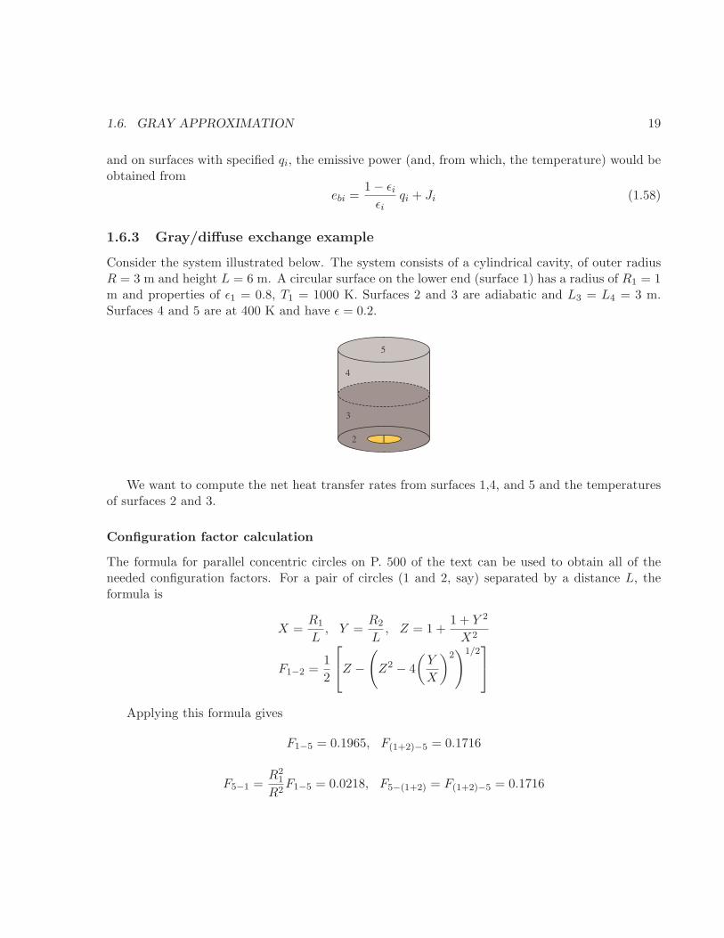
1.6.3 Gray/diffuse exchange example

Consider the system illustrated below. The system consists of a cylindrical cavity, of outer radiusR = 3 m and height L = 6 m. A circular surface on the lower end (surface 1) has a radius of R1 = 1m and properties of ǫ1 = 0.8, T1 = 1000 K. Surfaces 2 and 3 are adiabatic and L3 = L4 = 3 m.Surfaces 4 and 5 are at 400 K and have ǫ = 0.2.

12

3

4

5

We want to compute the net heat transfer rates from surfaces 1,4, and 5 and the temperaturesof surfaces 2 and 3.

Configuration factor calculation

The formula for parallel concentric circles on P. 500 of the text can be used to obtain all of theneeded configuration factors. For a pair of circles (1 and 2, say) separated by a distance L, theformula is

X =R1

L, Y =

R2

L, Z = 1 +

1 + Y 2

X2

F1−2 =1

2

Z −

(

Z2 − 4

(

Y

X

)2)1/2

Applying this formula gives

F1−5 = 0.1965, F(1+2)−5 = 0.1716

F5−1 =R2

1

R2F1−5 = 0.0218, F5−(1+2) = F(1+2)−5 = 0.1716


F5−2 = F5−(1+2) − F5−1 = 0.1497, F2−5 =R2

R2 − R21

F5−2 = 0.1685

Let surface 6 be the imaginary circular surface formed by the dotted line.

F5−6 = 0.3820, F1−6 = 0.4861

ThenF5−4 = 1 − F5−6 = 0.6180, F1−3 = 1 − F1−6 = 0.5139

F4−5 =R2

2RL4= 0.3090, F3−1 =

R21

2RL3F1−3 = 0.2855

By symmetry and summation,

F3−(1+2) = F4−5 = F3−1 + F3−2 : F3−2 = F4−5 − F3−1 = 0.2805

F2−3 =2RL3

R2 − R21

= 0.6311

Now use summation:

F1−4 = 1 − F1−5 − F1−3 = 0.2896, F5−3 = 1 − F5−4 − F5−2 − F5−1 = 0.2104

F2−4 = 1 − F2−5 − F2−3 = 0.2005

F4−1 =R2

1

2RL4F1−4 = 0.0161, F3−5 =

R2

2RL3F5−3 = 0.1052

F4−2 =R2 − R2

1

2RL4F2−4 = 0.0891

By the symmetry of the problem and summation,

F3−(1+2) = F4−5 = F3−1 + F3−2 : F3−2 = 0.2805

F2−3 =A3

A2F3−2 = 0.6311

What leaves 3 and lands on 6 (the imaginary surface) must land on either 4 or 5, so

F3−6 = F3−4 + F3−5

But F3−6 = F4−5 by symmetry, so

F3−4 = F4−5 − F3−5 = 0.2038 = F4−3

Only surfaces 3 and 4 can see themselves. Use summation:

F3−3 = F4−4 = 1 − F3−1 − F3−2 − F3−4 − F3−5 = 0.3820


Exchange equations

For surfaces 1, 4, and 5, upon which the temperature is specified, the exchange equations are

Ji − (1 − ǫi)N∑

j=1

JjFi−j = ǫiebi, i = 1, 4, 5 (1.59)

and on the adiabatic surfaces, 2 and 3, the exchange equations are

Ji −

N∑

j=1

JjFi−j = 0, i = 2, 3 (1.60)

The following is a listing of the Mathematica code used to solve the equations. I had previouslycalculated the configuration factors and stored them in the arrays f[i,j]. I use the symbol jf[i]for Ji in the code.

In[29]:=sigma=5.67*^-8;eps[1]=0.8;eps[4]=0.2;eps[5]=0.2;

t[1]=1000;t[4]=400;t[5]=400;

eb[1]=sigma t[1]^4;eb[4]=sigma t[4]^4;eb[5]=sigma t[5]^4;

In[37]:=vars=Table[jf[i],i,1,5]

Out[37]=jf[1],jf[2],jf[3],jf[4],jf[5]

In[40]:=eqns=Table[

If[i>1&&i<4,

jf[i]-Sum[jf[j] f[i,j],j,1,5]==0,

jf[i]-(1-eps[i])Sum[jf[j] f[i,j],j,1,5]==eps[i] eb[i]

]

,i,1,5]

Out[40]=

jf[1]-0.2 (0.513878 jf[3]+0.28963 jf[4]+0.196491 jf[5])==45360.,

jf[2]-0.631053 jf[3]-0.200488 jf[4]-0.168458 jf[5]==0,

-0.0285488 jf[1]-0.280468 jf[2]+0.618034 jf[3]-0.20382 jf[4]

-0.105197 jf[5]==0,

jf[4]-0.8 (0.0160906 jf[1]+0.089106 jf[2]+0.20382 jf[3]

+0.381966 jf[4]+0.309017 jf[5])==290.304,

-0.8 (0.0218324 jf[1]+0.14974 jf[2]+0.210393 jf[3]

+0.618034 jf[4])+jf[5]==290.304


In[42]:=soln=Solve[eqns,vars][[1]]

Out[42]=jf[1]->47060.5,jf[2]->8808.58,jf[3]->9753.96,

jf[4]->7088.69,jf[5]->7314.03

In[44]:=t[2]=(jf[2]/sigma)^(1/4)/.soln

t[3]=(jf[3]/sigma)^(1/4)/.soln

Out[44]=627.814

Out[45]=644.02

In[48]:=

q[1]=eps[1]a[1]/(1-eps[1])(eb[1]-jf[1])/.soln



Out[48]=121133.

Out[49]=-79693.6

Out[50]=-41439.7

In[51]:=q[4]+q[5]

Out[51]=-121133.

Documents

Radiation Exchange Between Surfaces - Auburn Universitydmckwski/mech7210/radexchan… · · 2007-03-15Radiation Exchange Between Surfaces 1.1 Motivation and Objectives Thermal radiation,