Inverse modelling for source term reconstruction

Radek Hofman

University of Vienna, Department of Meteorology and Geophysicsradek.hofman@univie.ac.at

http://homepage.univie.ac.at/radek.hofman/

20 Oct 2014, ČSKI seminar, UTIA AV ČR v.v.i

Introduction

I Goals and example applicationsI Inverse modeling ingredients

I Atmospheric transport modeling

I Methodology and state-of-artI Real world example - analysis of measurements from IMSI Conclusion

Inverse modelling - Goals

I The ultimate goal of the inverse modelling is to provide asource-term estimate based on analysis of measurements andtheir systematic comparison with results of atmosphericdispersion modelling (optimization of model parameters)

I This has many applications of different purposes and variouscomplexity

Applications: Emissions of greenhouse gasses

I Backtracking of emissions of trace species (e.g. halogenatedhydrocarbons like CFCs) using atmospheric transport modeling tocountries of their likely origin and estimation of release magnitudes

I Comparison of emissions reported from European countries withobservations — multiple sources with unknown time profiles

From: Keller, Christoph A., et al. "European emissions of halogenatedgreenhouse gases inferred from atmospheric measurements." Environmentalscience & technology 46.1 (2011): 217-225.

Applications: Emissions of ash from volcanoesI Estimation of ash emission from volcanoes for purposes of aviation using

satellite observations — known source location, unknown time and heightprofile

From: Stohl, A., et al. "Determination of time-and height-resolved volcanic ashemissions and their use for quantitative ash dispersion modeling: the 2010Eyjafjallajökull eruption." Atmospheric Chemistry and Physics 11.9 (2011)

Applications: Nuclear applications — nuclear accidents

I Estimation of emissions from Fukushima accident usingnuclide-specific observations — known source location,unknown time and height profileE.g.: Stohl, A., et al. "Xenon-133 and caesium-137 releases into theatmosphere from the Fukushima Dai-ichi nuclear power plant:determination of the source term, atmospheric dispersion, anddeposition." Atmospheric Chemistry and Physics 12.5 (2012): 2313-2343.

I Estimation of emissions from Fukushima accident using bulkgamma dose rate observations (more common, higher timeresolution, no nuclide information) — known source location,unknown time and height profile, source composition, isotoperatiosSaunier, Olivier, et al. "An inverse modeling method to assess the sourceterm of the Fukushima Nuclear Power Plant accident using gamma doserate observations." Atmospheric Chemistry and Physics 13.22 (2013):11403-11421.

Applications: Nuclear applications — verification of CTBTI Verification of the CTBT (Comprehensive Nuclear-Test-Ban Treaty) by

the means of CTBTO Int. Monitoring System (IMS) (Operationallyestimated possible source regions using correlations of samples withsource sensitivities)

I Unknown source location, unknown time and height profile of source,background sources cluttering useful signal

Inverse modelling — basic ingredients

I Set of observation (and their error statistics)I Results of atmospheric transport modeling (and corresponding

error statistics)I Prior information about the source: source type (e.g. point

source), location, magnitude of release, effective release height(and corresponding error statistics)

I A metric quantifying compatibility between measured data andsource hypothesis (cost function, likelihood, KL-divergenceetc.)

Atmospheric transport modelling (ATM)

I Let xT = [x1, . . . , xI ] be a vector of sources characterized bytheir spatial-temporal characteristics (a point forpoint-sources/3D grid cell for volume sources and a releasetime interval) and yT = [y1, . . . , yJ ], be a set ofobservations—sampling points given their location andsampling time (interval). A general atmospheric chemistrytransport model can be understood as a non-linear operatorM(·) transforming sources to measurements

y =M(x) + ε.

I ε is an overall error caused by measurements errors, dispersionmodel imperfection, errors in its inputs includingmeteorological fields etc.

ATM: Source-receptor sensitivity

I Important concept in air quality modeling describing thesensitivity of a receptor to a source

I Source-receptor sensitivity of j-th sample and i-th source isdefined

mij =∂yj∂xi

I For a linear modelM, i.e. passive tracers and substanceswhich do not undergo nonlinear chemical transformation(advection and dispersion is a linear process) and substanceswith a prescribed decay or growth rate (e.g. radioactive decay):

mij =yjxi

ATM: Source-receptor sensitivity

I Given a source-receptor matrix M ∈ RI×J , the resultingreceptor values can be obtained simply by matrix-vectormultiplication, avoiding evaluation of the whole model ⇒ frommathematical point of view the problem is fully described byM, y and (optionally) their error statistics and a prior

Mx = y

I Unfortunately, the system is often ill-conditioned and cannotbe solved for x

I How to obtain M?

ATM: Eulerian vs. Lagrangian models

From D. Arnold, FLEXPART training course 2013

ATM: Eulerian vs. Lagrangian models

From D. Arnold, FLEXPART training course 2013

ATM: Lagrangian transport modellingI PROs:

I Can be computationally very efficient (depending on size ofplume): only the fraction covered with particles is simulated

I Turbulent processes are included in a more natural way unlikeEulerian models

I There is no numerical diffusion due to a computational gridI Many first order processes can be easily included with a

prescribed rate: radioactive decay, dry deposition, washout,etc.

I One particle can carry more than one speciesI Better for treatment of point sources and receptors

I CONs:I It is quite difficult and computationally expensive to include

non-linear chemical reactions (also in Eulerian, ∆t ∼ reactionspeed)

I To do the chemistry in LPDM we have to do an intermediategridding to get concentrations and then redistribute particlesagain, so we loose advantages of Lagrangian approach.Normally, we do the gridding only at the end.

ATM: Forward vs. backward calculation

From: Seibert, P., and A. Frank. "Source-receptor matrix calculation with aLagrangian particle dispersion model in backward mode." AtmosphericChemistry and Physics 4.1 (2004): 51-63.

ATM: Forward vs. backward calculation

I Forward is beneficial when we have more samples thanpotential source

I Backward is beneficial when we have more potential sourcesthan samples

I Lagrangian ATM:I Forward run: particles released from sourcesI Backward run: models is “self-adjoint”—particles released from

receptors with negative time sign

I Eulerian ATM:I Forward run: solving forward model with different right hand

sides as many times as the size of control vector xI Backward run: solving adjoint equations with different right

hand sides as many times as the size of measurement vector y

Parametrization of a source

I Source can be viewed as a mapping s(x , y , z , t) : R4 → RS ,where x , y , z are spatial coordinates, t is time and S is anumber of species emitted

I Each time slot/spatial grid cell is a random quantityI E.g.: a source at know location with unknown emission

height/time can be parametrized as a source with possibleemissions from different heights at different times:xT = [xz=1,t=1, . . . , xz=Z ,t=1, . . . , xz=1,t=T , . . . , xz=Z ,t=T ],i.e. we need SRS of measurements to all possibleemission heights and times where z and t are suitablediscretized

I Large number of unknowns ⇒ usually leads to anill-conditioned problem which must be heavily regularized

ATM FLEXPART

I A notable representative of the family of Lagrangian modelsI Lagrangian particle dispersion model developed maintained

mainly at NILU Norway (http://flexpart.eu/)Stohl, A., Markus Hittenberger, and Gerhard Wotawa. "Validation of theLagrangian particle dispersion model FLEXPART against large-scaletracer experiment data." Atmospheric Environment 32.24 (1998):4245-4264.

I > 35 users from > 15 countriesI Released under the GNU General Public License V3.0I Evaluates dosimetric quantities in post-processingI Two main alternative meteorological inputs:

I ECMWF data http://www.ecmwf.int/I US National Weather Service - GFS data, available for

download from http://nomads.ncdc.noaa.gov/

ATM: How to estimate model error?I Model error often much more significant (higher) than the

measurement errorI Critical particularly near the “edge of a plume”I How to estimate it?

I Assume model error proportional to measured value - a verypoor man’s approach

I Estimate “local error statistics” of a measurement usingsamples of model results around receptors - poor man’sapproach (uncertainty in wind field, not in turbulenceproperties)

I Difference between forward and backward runsI Ensemble approach — model error is estimated using an

ensemble of INDEPENDENT and REPRESENTATIVE modelruns. This assumption is not fulfilled in real world applications(models similar with common “parents”) and an ensembleshould be inspected in terms of member covariance before use,see Potempski and Galmarini (2009)

I Estimation of model error using hyper-parametrized models

ATM: How to estimate model error?Different ensemble types:

From Galmarini et al. (2004)

Inverse modelling for source reconstruction — Methodology

1. Optimization approaches: ||y −Mx||2 → min by the means ofsolution of (ill-conditioned) system of linear equations

2. Fully Bayesian solution: Let p(x) and p(y) be probabilitydensity functions (pdfs) of vectors x and y, respectively:

p(x|y) =p(y|x)p(x)

p(y)=

p(y|x)p(x)´p(y|x)p(x)dx

∝ p(y|x)p(x).

I The goal is to obtain posterior distribution p(x|y)I How? Different approaches for with different assumptions

suitable for different scenarios and of a different complexityI Analytical approaches (conjugate distributions)I Approximate sampling-based approaches

I Sometimes, these two approaches are equivalent, as we willsee...

Inverse modelling — Variational approachI If both likelihood function p(y|x) and prior p(x) are assumed

to be Gaussian: p(y|x) = N (Mx,R), p(x) = N (xa,B), thenMaximum A-Posteriori (MAP) estimate can be obtained as themode of the posterior

x̂ = argmaxx

(p(y|x)p(x))

I This is equivalent to

x̂ = argmin(0.5(y −Mx)TR−1(y −Mx) + 0.5(x− xa)TB−1(x− xa) + const

).

I R and B represent error covariances of observations and sourceprior (usually assumed to be diagonal)

I Observation error contains not only measurement error itselfbut it should contain also a model error caused by wrongconceptualization of a physical phenomena in the model

R = Rmod + Rmea

Inverse modelling — Variational approach

J1(x) = (y −Mx)TR−1(y −Mx)︸ ︷︷ ︸model-obs mismatch

+ (x− xa)TB−1(x− xa)︸ ︷︷ ︸regularisation w.r.t prior

→ 0

I The first term on r.h.s measures deviations of model fromobservations and the second term acts as a regularization andmeasures deviation of source hypothesis from prior xa (analogyto Tikhonov regul.)

I Minimization can be done analytically by ∂J∂xi

!= 0, i = 1, . . . , I

I We solve the following system for x:

(MTR−1M + B−1)(x− xa) = MTR−1(y −Mxa)

I A-posteriori error

P = (MTR−1M + B−1)−1

Variational approach — Regularization

I We can impose also additional types of regularization(cost function does not need to be quadratic then):

I quadratic cost ⇒ analytical minimization: Stohl,A., et al. "Xenon-133 and caesium-137 releases into theatmosphere from the Fukushima Dai-ichi nuclear power plant:determination of the source term, atmospheric dispersion, anddeposition." Atmospheric Chemistry and Physics 12.5 (2012):2313-2343.

I numerical minimization: Saunier, Olivier, et al. "Aninverse modeling method to assess the source term of theFukushima Nuclear Power Plant accident using gamma doserate observations." Atmospheric Chemistry and Physics 13.22(2013): 11403-11421.

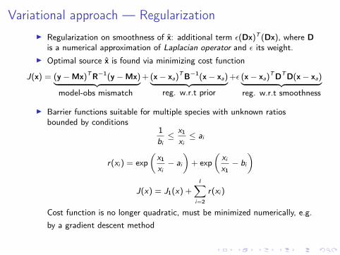
Variational approach — RegularizationI Regularization on smoothness of x̂: additional term ε(Dx)T (Dx), where D

is a numerical approximation of Laplacian operator and ε its weight.I Optimal source x̂ is found via minimizing cost function

J(x) = (y −Mx)TR−1(y −Mx)︸ ︷︷ ︸model-obs mismatch

+(x− xa)TB−1(x− xa)︸ ︷︷ ︸reg. w.r.t prior

+ε (x− xa)TDTD(x− xa)︸ ︷︷ ︸reg. w.r.t smoothness

I Barrier functions suitable for multiple species with unknown ratiosbounded by conditions

1bi≤ x1

xi≤ ai

r(xi ) = exp(x1

xi− ai

)+ exp

(xix1− bi

)

J(x) = J1(x) +I∑

i=2

r(xi )

Cost function is no longer quadratic, must be minimized numerically, e.g.by a gradient descent method

Inverse modelling — Bayesian approach

I Sampling (brute force) approachI Hierarchical models — hyper-parameters of anythingI Variational BayesI Marginalized models ... and many more

Examples:I MLE on hyperparameters: Winiarek, Victor, et al. "Estimation of the

caesium-137 source term from the Fukushima Daiichi nuclear power plantusing a consistent joint assimilation of air concentration and depositionobservations." Atmospheric Environment 82 (2014): 268-279.

I MCMC: A. Ganesan, M. Rigby, A. Zammit-Mangion, A. Manning, R.Prinn, P. Fraser, C. Harth, K.-R. Kim, P. Krummel, S. Li & others,Characterization of uncertainties in atmospheric trace gas inversions usinghierarchical Bayesian methods, Atmospheric Chemistry and Physics 14,3855-3864 (2014)

I sequential MC: Šmídl, Václav, and Radek Hofman. "Efficient SequentialMonte Carlo Sampling for Continuous Monitoring of a RadiationSituation." Technometrics (2013), doi 10.1080/00401706.2013.860917

Conclusion

I The spectrum of methods spans from simple regression toadvanced Bayesian methods

I The problem can be reduced to linear algebra operations —what we need is just a SRS matrix, corresponding vector ofobservations (optionally their error statistics and a prior)

I Different datasets are available, e.g., in a database hosted atNILU: http://actris.nilu.no/

Real life application:

Analysis of the April 2013 radioxenondetections based on formal inverse modeling

Radek Hofman and Petra Seibert

University of Vienna,Department of Meteorology and Geophysics

23 Sep 2014, ATM workshop 2014, Stockholm, Sweden

Objectives

I Our goal is to analyze 3 significant 133Xe detections made 7–9April 2013 at Takasaki station (JPX38, CTBTO IMS)

I We attempt to estimate time- and height-dependent sourceshapes using a cost function based inverse modeling technique

I Scenarios with both known and unknown source location arestudied

I Demonstration of fusion with waveform events of period of 30Jan – 26 Feb 2013

Samples included into inversionI Triggering samples — 3 significant JPX38 detections:

I 08 April 2013 06:54 UTC collection stopI 08 April 2013 18:53 UTC collection stopI 09 April 2013 06:54 UTC collection stop

I Other relevant samples (incl. nondetections to confine the source)— samples spatially and temporally adjacent:

I Spatially we include additional samples from 5 adjacentstations (RUX58, MNX45, CNX20, CNX22 and USX77)

I Temporally ±1 sampling period for JPX38 and ±2 otherwise

Samples included into inversion – SummaryI 36 detections and nondetections enter source inversion algorithm

where systematically compared with atmospheric transport modelingto give us some inference about the source (location, strength...)

0.00

0.15

0.30

(mBq/m

3)

CNX20

bg.

0.00

0.15

0.30

(mBq/m

3)

CNX22

bg.

Apr 05 Apr 07 Apr 09 Apr 11 Apr 13 Apr 150.00

1.50

3.00

(mBq/m

3)

JPX38

bg.

0.00

0.15

0.30MNX45

bg.

0.00

0.06

0.12RUX58

bg.

Apr 05 Apr 07 Apr 09 Apr 11 Apr 13 Apr 150.00

0.03

0.06

USX77

bg.

10°N

20°N

30°N

40°N

50°N

60°N

80°E 90°E 100°E 110°E 120°E 130°E 140°E 150°E 160°E 170°E 180° 170°W 160°W 150°W

MNX45

CNX22

CNX20RUX58

JPX38

USX77

DPRK test site

sampling station

Atmospheric transport modelingI Source-receptor sensitivities (SRS) calculated using backward

runs of FLEXPART 9.0I 36 samples = runs, each with 1 mio particles, ≤15 days backI SRS calculations performed with high accuracy:

I ECMWF input data 0.25◦ horizontal resolution, 91 verticallevels, 3 h temporal resolution

I FLEXPART output on lon-lat grid with ∆x = 0.25◦ and∆y = 0.2◦ every 3 hours

I Convection enabled in FLEXPART

I We assume 5 vertical layers in order to account for complexterrain at the DPRK test site which varies between 500 and2200 m asl: 0–100 / 100–500 / 500–1000 / 1000–1500 /1500–2000 m (metres above model ground), model ground is880 – 1500 m asl

I We assume point releases only (from a single grid cell –implicit a-priori knowledge)

Inversion methodology

I Estimation of temp. shape of a release in 5 vertical layers over≈ 15-day time window: 121 possible 3-hour release intervals× 5 vertical layers = 605 unknowns

I Problem is ill-conditioned – data do not constraint enough allelements of the source vector x ⇒ we need regularization

I Solution is found via minimizing the cost function

J(x) = (y −Mx)TR−1(y −Mx)︸ ︷︷ ︸model-obs mismatch

+ (x− xa)TB−1(x− xa) + ε(Dx)T (Dx)︸ ︷︷ ︸regularisation

I Model error estimated using “pseudo-ensemble” of model runs(SRS shifted in time and space) and added to obs. error

I First-guess solution xa = 1 · 103 Bq (≈ 0); σx = 3 · 1011 Bqper element of solution vector, thus total can be larger

I Negative parts of solution were suppressed via iterative processreducing first-guess error for appropriate solution parts

Case 1: Cont. release at DPRK test site – temp. shapeI Simultaneous estimation of the source strength as a function of

release time and heightI Addition of non-detections suppressed releases at the beginning of

assumed interval

0.0

0.5

1.0

1.5

2.0

Rele

ase

(B

q)

1e11 Only 5 JPX38 samples, total release 3.41E+11 Bq

layer 5 - 3.42E+10 Bq

layer 4 - 7.14E+10 Bq

layer 3 - 1.76E+11 Bq

layer 2 - 4.21E+10 Bq

layer 1 - 1.85E+10 Bq

Mar 28 Mar 30 Apr 01 Apr 03 Apr 05 Apr 07 Apr 09 Apr 110.0

0.5

1.0

1.5

2.0

Rele

ase

(B

q)

1e11 All 36 samples, total release 4.10E+11 Bq

layer 5 - 1.41E+10 Bq

layer 4 - 9.47E+09 Bq

layer 3 - 2.72E+11 Bq

layer 2 - 1.06E+11 Bq

layer 1 - 8.78E+09 Bq

Case 1: Agreement of retrieved STs with observations

10-6 10-5 10-4 10-3 10-2

Simulations (Bq/m3 )

10-6

10-5

10-4

10-3

10-2

Obse

rvati

ons

(Bq/m

3)

Real vs. simulated observations(5 JPX samples only)

10-6 10-5 10-4 10-3 10-2

Simulations (Bq/m3 )

10-6

10-5

10-4

10-3

10-2

Obse

rvati

ons

(Bq/m

3)

Real vs. simulated observations(all 36 samples)

Case 1: Cont. release at DPRK test site – vertical profileI Important to use elevated releaseI Main release 100–1000 m agl (model)I Corresponds roughly to 1000-2500 m asl – quite reasonable

0.0e+00 1.0e+11 2.0e+11 3.0e+11source strength (Bq)

0

500

1000

1500

2000h

eig

ht

(m a

bo

ve

mo

de

l g

rou

nd

)

Release as function of height

Case 2: Cost function all over the domainI Test each grid cell as an independent candidate source, determine

release time/shape by inversion and plot cost function per grid

20°N

30°N

40°N

50°N

60°N

110°E 120°E 130°E 140°E 150°E 160°E 170°E

CNX22

CNX20

USX77

JPX38

RUX58

Spatial cost J(x)

DPRK test site, J(x)=4.18sampling stationJ(x) min=0.62

100

101

102

Case 2: Cost function all over the domain

I Oceans masked

20°N

30°N

40°N

50°N

60°N

110°E 120°E 130°E 140°E 150°E 160°E 170°E

CNX22

CNX20

USX77

JPX38

RUX58

Spatial cost J(x)

DPRK test site, J(x)=4.18sampling stationJ(x) min=0.62

100

101

102

Fusion with possible sources – Method

I Select a list of relevant seismic events (time period, region)I Here: 193 seismic events from 30 Jan – 26 Feb 2013 in our

inversion domain

I Select other possible sources of emissions (medical isotopeproduction facilities, NPPs...)

I Here: 10 NPPs from China, Taiwan, South Korea and Japan(the only operating nuclear power plant in Japan during thetime of interest was NPP Ohi)

I Attribute cost function value to all assumed 203events/sources based on their location (in which grid cell(s)they fall)

I Exclude events which fall into regions with high cost functionI Plot/rank remaining events by their cost function value

Fusion with possible sources – ResultI Cost function in the background as grayscaleI Ellipses surrounded by circle coloured with the cost at ellipse centreI NPPs marked by pentagons coloured with the cost at NPP site

20°N

30°N

40°N

50°N

60°N

110°E 120°E 130°E 140°E 150°E 160°E 170°E

CNX22

CNX20

USX77

JPX38

RUX58

Spatial cost and possible radioxenon sources (seismic events + NPPs)

DPRK test site, J(x)=4.18sampling stationJ(x) min=0.62

100

101

102

100 101 102

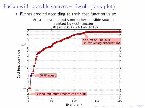
Fusion with possible sources – Result (rank plot)I Events ordered according to their cost function value

0 50 100 150 200

Event rank

100

101

102

Cost

funct

ion v

alu

e

DPRK event

Global minimum (regardless of SHI)

Saturation - no skill in explaining observations

Seismic events and some other possible sourcesranked by cost function

(30 Jan 2013 - 26 Feb 2013)

Fusion with possible sources – Result (rank plot)I Closer look on events with lowest cost function values

I Currently, cost function values taken from a single point (ellipsecenter) — this can lead to misclassification of an event (red andgreen ellipses), maybe some averaging (smoothing) appropriate

Conclusions of experiment

I The DPRK test 2013 / April 2013 Xe-133 detections wereused as a test for inverse-modelling based source location andquantification

I The problem is heavily ill-conditioned (36 samples, mostlynon-detections, 605 unknowns), regularization methods forobtaining physically reasonable solution must be employed.

I Release shape estimated using different variants of the methodis consistent and appears to be a stable feature

I Magnitude of release (≈ 4E11 Bq) is lower than previouslysuggested due to different inversion strategy and settings

I Might be influenced by regularization, further tests needed

I DPRK test site is among the region of lower cost functionthough not at the global minimum

Conclusions (2) – Fusion

I Cost function from the inversion can be used as a measure ofcompatibility between assumed source location and observedradionuclide concentration — regions with low cost functionare possible source regions

I Because of the uncertainties involved, the source does notneed to be in the very minimum of the cost function

I The source was found to be associated with the 5th lowestcost function among all the assumed sources in the timewindow considered

I By clipping events at some value of the cost function, thenumber of candidate events could be reduced substantially

I Of course, many possibilities exist for refinements andextensions

Options for future improvements

I Better quantification of errors both for the input and theresults

I Use different resolution of met. data and SRS data for ATMuncertainty quantification

I Use ensemble of SRS data from different transport modelsI Include off-diagonal terms in error covariance matricesI Work on quantifying background uncertaintyI Experiment more with regularisation

I Try to include known background radioxenon sources intoinversion

I Try also inversion of 131mXe dataI Do next iteration of relevant RN samples which could be

useful for narrowing down further the likely source regions

Thank you!

Acknowledgements:

Research was supported by FP7 project PREPARE — Innovativeintegrative tools and platforms to be prepared for radiologicalemergencies and post-accident response in Europe

Data were provided by the Preparatory Commission for theComprehensive Nuclear-Test-Ban Treaty Organization (CTBTO).This work contains only opinions of the authors, which can not inany case establish legal engagement of the Provisional TechnicalSecretariat of the CTBTO.