RADAR RESPONSE OF VEGETATION: 5/2.

AN OVERVIEW N 9 4 -/_. _ _;:_

[

Fawwaz T. Ulaby and M. Craig DobsonThe University of Michigan

• Vegetation Classes

• Soil Scattering: (1) Backscatter(2) Forward Scattering

• Radar Response

• Vegetation Biomass

• Vegetation Structure

• Temporal Variations: (1) Short Term (hours to days)(2) Long Term (Seasonal)

• Effect of Rain

• Emergence of a User Community

• Concluding Remarks

jThe University of Michigan

- 151

https://ntrs.nasa.gov/search.jsp?R=19940011425 2019-08-25T07:26:44+00:00Z

0

152

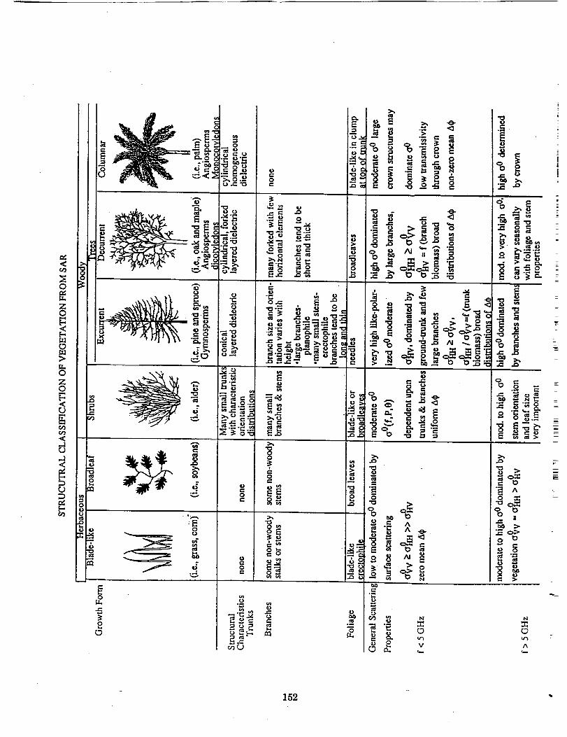
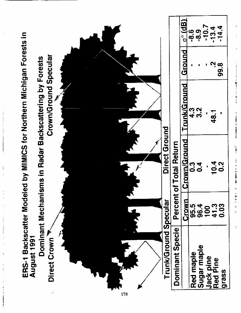
RADAR SCA'I-I'ERING MECHANISMS

Direct Crown

Vegetation-Ground

Direct Ground

• Direct Ground Backscatter

• Vegetation-Ground BistaticScattering• Trunks• Leaves (needles)• Branches

• Direct Crown Backscatter

153

University ofMichigan J

MOD-3

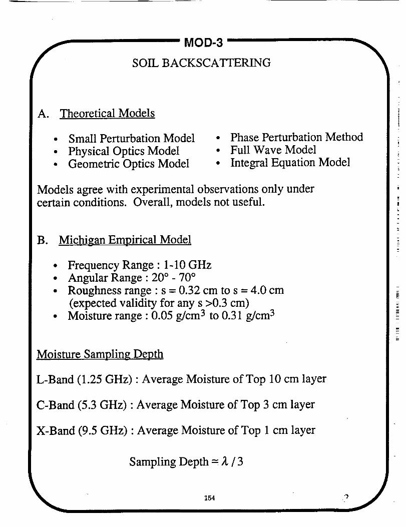
SOIL BACKSCATTERING

A. Theoretical Models

• Small Perturbation Model

• Physical Optics Model• Geometric Optics Model

• Phase Perturbation Method• Full Wave Model

• Integral Equation Model

Models agree with experimental observations only undercertain conditions. Overall, models not useful.

B. Michigan Empirical Model

• Frequency Range : 1-10 GHz• Angular Range :20 °- 70 °• Roughness range : s = 0.32 cm to s = 4.0 cm

(expected validity for any s >0.3 cm)• Moisture range : 0.05 g/cm 3 to 0.31 g/cm 3

Moisture Sampling Depth

L-Band (1.25 GHz) : Average Moisture of Top 10 cm layer

C-Band (5.3 GHz) : Average Moisture of Top 3 cm layer

X-Band (9.5 GHz) : Average Moisture of Top 1 cm layer

Sampling Depth = Z / 3

154 o

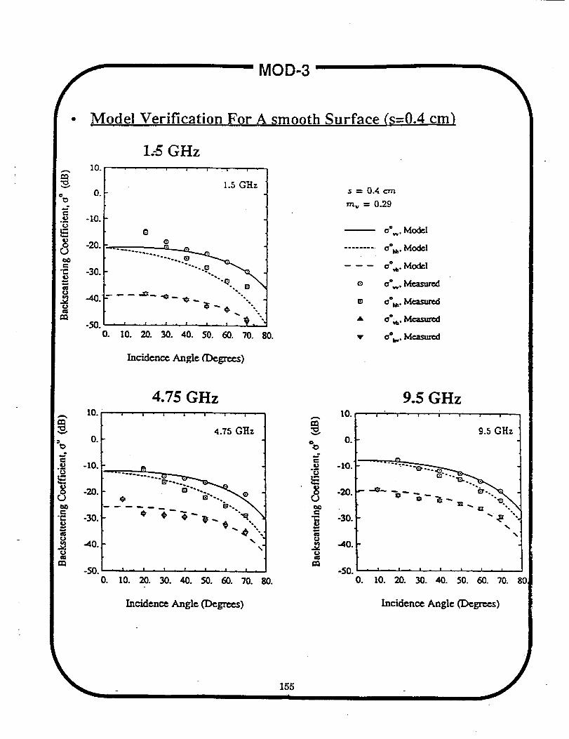
M MOD-3odel Verification For A smooth Surface (s=0.4 cm)

c o

c

¢o

u

1.-5GHz

1.5 Gllz0.

-I0.

-20. e

-30. "'"-..m

-40. -- -- -_-- _a-- _ "'.

",-50. " ........ ' ' • --

0. 10. 20. 30. 40. 50. 60. 70. 80.

Incidence Angle (Dcgrce_s)

5 = 0.4 cm

m,, = 0.29

o°.. Model

.........a°_. Model

o°.. Model

m o°_,.Mcasua=:l

A oe_,_

v o°_. Mcaau_

4.75 GHz10. - 4 "-

9.5 GHzI " I " | " 4 " i " i -

9.5 GHz

N.

0 . i . I . I . ! . ! . ! - !

O. 10. 20. 30. 40. 50. 60. 70. gO,

Incidence Angle (Degrees) Incidence Angle ('Degrees)

¢II

4.0

®

3.0

2.0

1.0

0.00.0

MOD-3

I ' i

correl, coeff. = 0.98

1990 meas.

1991 meas.

E3/

/

® ®i_ /® /®

/ / I':1

N,

Bs"

//

B /®/

/

/

/

/

/

/

I

1.0

/

7

I

3.0

/

1:1 //

/I

/7

rms height

4.0

Measured ks

o

0.4

0.3

0.2

0.1

/

0.0'0.0

®

B

I

I

I

/

I

I ' I

correl, coeff. = 0.97

1990 meas.

1991 me,as.

®/

&.,B /

/13

/

I , !

0.1 0.2

| = l:

It

El //

/

J

/

//

,,NO/

0.4

soil moisture

Measured m v156

MOD-3

A

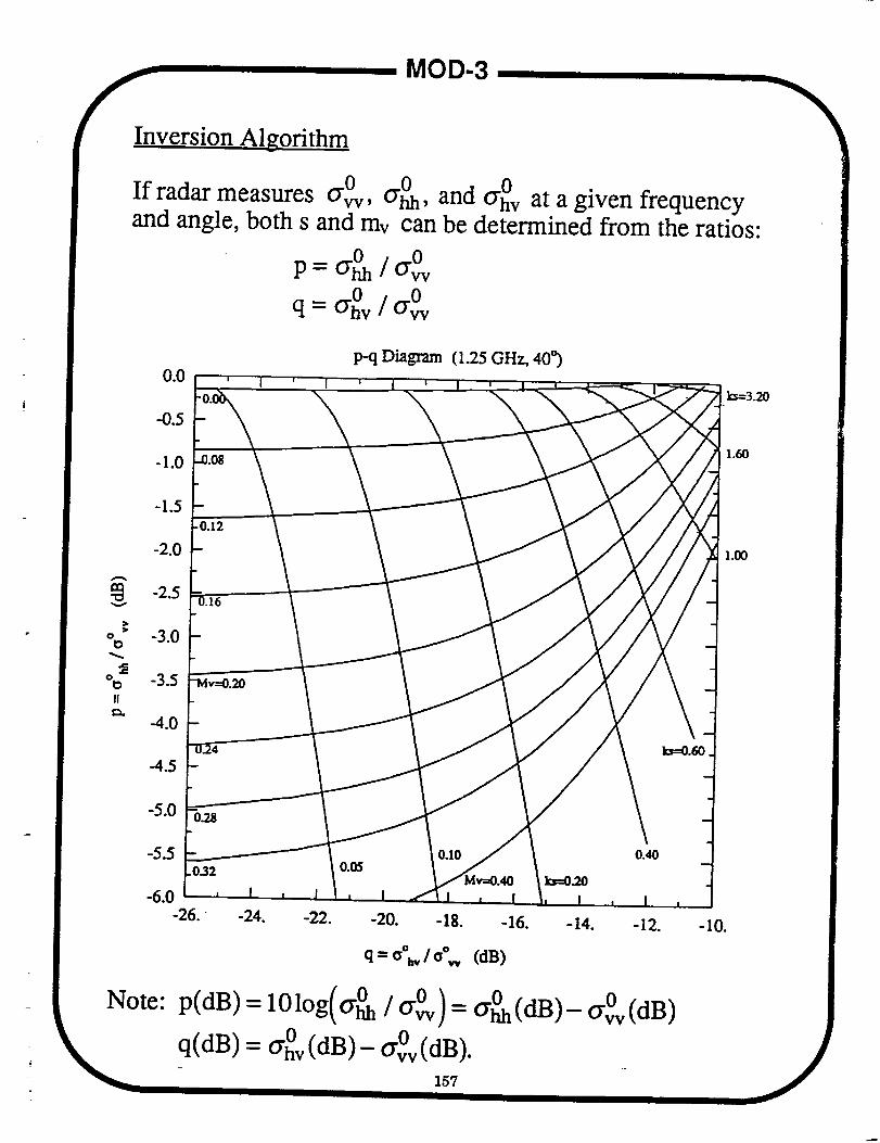
Inversion Algorithm

If radar measures o"O, o"O, and O-°v at a given frequencyand angle, both s and mv can be determined from the ratios:

p=a°/o °

q= a°v/a °

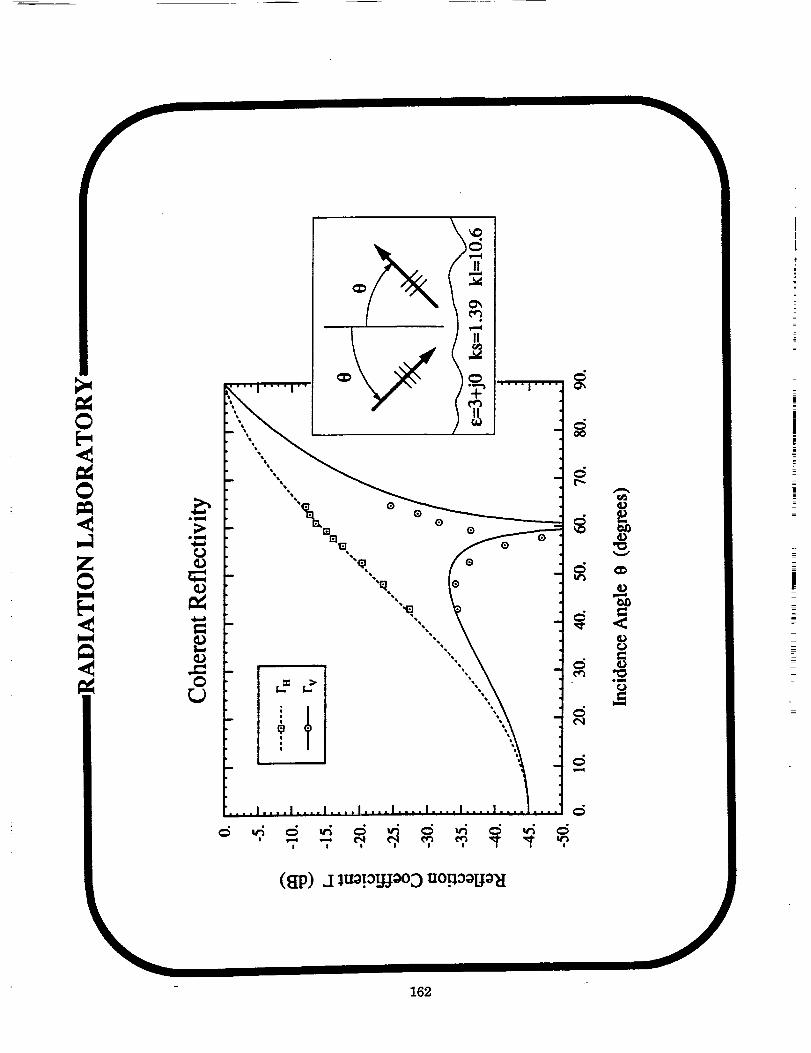
p--q Diagram (1.25 GHz, 40*)

ks=3.20

1.60

O

%IIe_

1.00

0.40

q= o°,../a'...(riB)

Note: p(dB)= 1010g(G O / G°)= o-O(dB)_ GO(dB)

q(dB) = G°v (dB)- o-v°(dB).

157

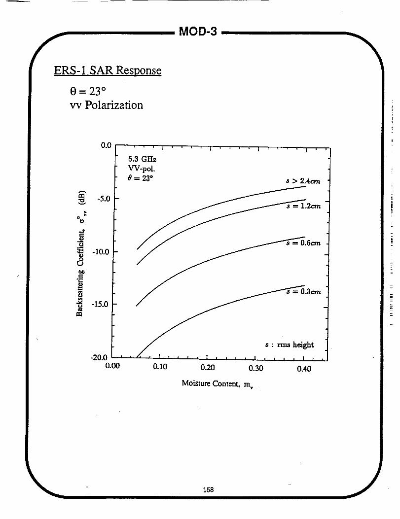
MOD-3

ERS- 1 SAR Response

0= 23 °vv Polarization

5.3 Cl:/z

W-pol.

#=23* s > 2.4era

-5.01.2ern

-20.0

0.00

s : rms height

I I ! ! ! l i i w , I. i t • J I , I

0.10 0.20 0.30 0.40

Moisture Content, m v

- 158

159

• |

J

||

|

!

IE

=

Z

Z

160

II IIII

!J

|

t_

!lm

m

_. .._....i...._....l....t....j...._....

I ! I ! ! I

!

d

161

162

I

iiiii

163

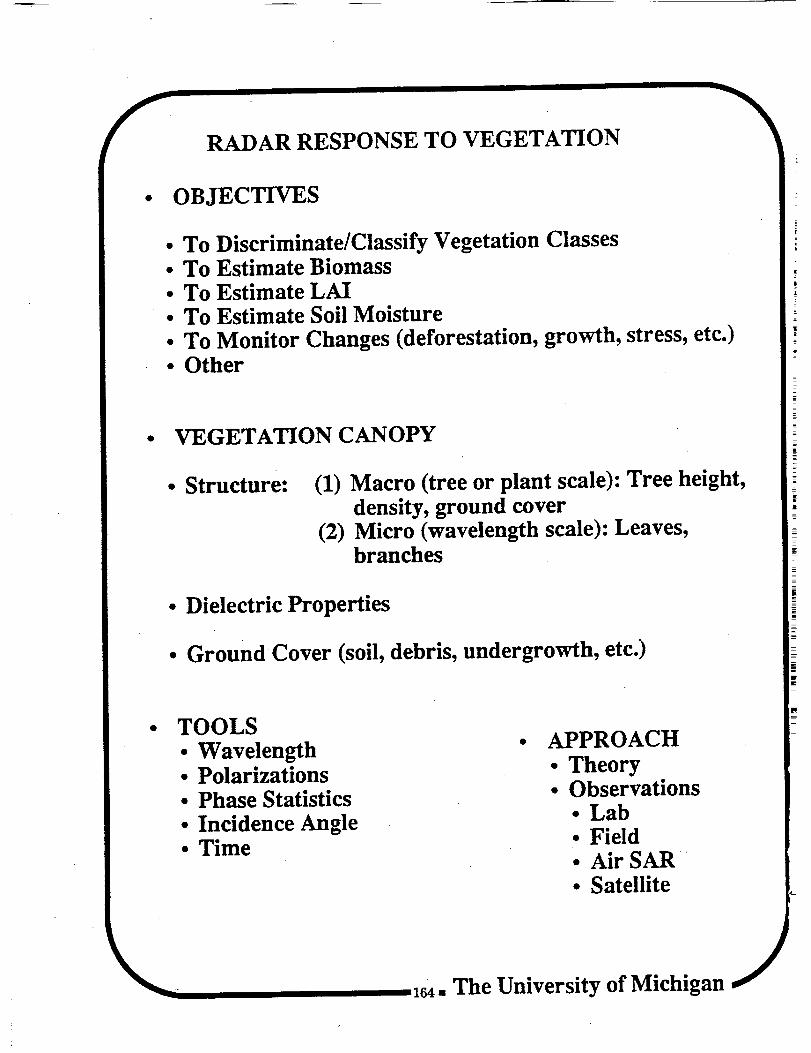
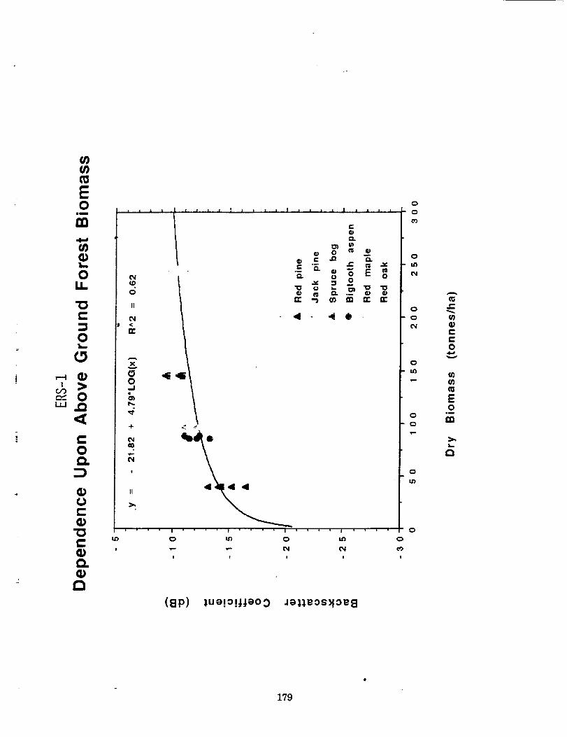
RADAR RESPONSE TO VEGETATION

• OBJECTIVES

• To Discriminate/Classify Vegetation Classes• To Estimate Biomass• To Estimate LAI• To Estimate Soil Moisture• To Monitor Changes (deforestation, growth, stress, etc.)• Other

• VEGETATION CANOPY

• Structure: (1) Macro (tree or plant scale): Tree height,density, ground cover

(2) Micro (wavelength scale): Leaves,branches

• Dielectric Properties

• Ground Cover (soil, debris, undergrowth, etc.)

• TOOLSWavelength • APPROACH• Polarizations • Theory• Phase Statistics • Observations• Incidence Angle • Lab• Time • Field

• Air SAR _

• Satellite __

164. The University of Michigan

°°_"" /// I

l!io.,. -_ f'of _" ri/i. t"_ i s 2

I i , 4i.ol i. L:"o,_ _ I"

/Tf = = " -0, -'. _."

.// 0 • .... i _ _ _ . ! .... | .... i

•I ._ _" /"

0,

° "_ I l=_ _ ,"T o /

I" ol ..t /"

_ ..._ C_l l t1

•.= "- -" ,,, c/ =\ /"

o ,_.... _ .... =. _.-165 0,,0 (SZp) =_-aTo'l:;.;aoD =aoa_os_1o_

t.¢#

¢¢

¢¢

t..

m

I00"

I0

.I

.01t

0

0100

10

.1

.01

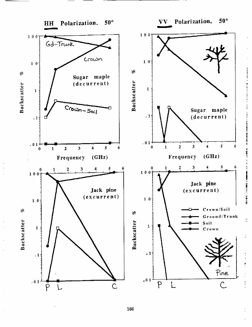
HH Polarization. 50 °

G 3 -9-ru_,K-

Sugar maple

(decurrent)

Il

1 2 3 4 5 6

Frequency (GHz)

1 2 3 4 5 6

C

t_

L

¢,#

100

10

.1

.010

0100

10

VV Polarization, 50 °

_ Sugar maple

V", urret• --i • I ' a - I " i "

1 2 3 4 5

Frequency (GHz)

1 2 3 4 5

Jack pine

(excurrent)

? L

Crown._Soil

Ground:'Trunk

Soil

Crown

=

i[[

!

C

166

° 5'

m-o

c -I0

(J.DM,,--

-15O0

i,._

20

O(/)

(.> -25

IZI

-3O

| , !

HH Polarization

0.44 1.2 5.3

-10

"-" -15m"0

c -20

=m

0,m

-25O

O

m -304d

(J

(.) -35"

-4O

HV Polarization

0.44 1.2 5.3

Frequency (GHz) Frequency (GHz)

nn"O

O=u

n-

-r--r-

0.448

6

4

2

0

- 2'

- 4 . 0

1.2 5.3I i I

•-,-4b--- Herbaceous

Slash

Excurrent LP

Excurrent RP

Decurrent RM

HH/VV Ratio

0 _ i

L C_.

167

A

m-o

om

t_rr

-I-

-I-

15

10

5

0.44 1.2 5.3I , I , i

HH/HV Ratio

m i i

p L C_..

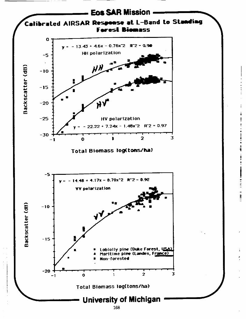
Eos SAR Mission

CalibraLed AIRSAR lles4_a_J4 at L-Band Lo StaaMiag_IFoc_IL Bieiass

0

y = - 13.43 + 4.6x - 0.76x'2

HH polarization

HV polarization

y = - 22.22 ÷ 7.24x - 1.48x'2

• . | . • w • I • • •

0 !

R-2 = 0.97

I,

2 3

Total Biomass Iog(to_>/l_a)

y = - 14.48 * 4.17x - 0.70x'2

VV pelartzation

i

!

• Loblolly pine (Duke Forest,• Maritime pirm (Lae<les, France)• Non-forested

Total Biornass log(tons/ha)

University of Michigan168

i

F 2

el IdrL • OU] ._ .._ .._ ..; .._ 0

_,_ _ °°°• D _ > •

D -r" > =

fIrC _= i

.J

mm

0m

0

E.Et_

_-E_ em

"" 4=' L

p) 0!o!_ o:) u!Jol os)l:

O | , J , I . | - • i .... i .... i .... I .... [ ....

i .,o° q7 _ q7

ii II I]LN _ eq

° ' "ll_ "=_t 4o4n oc] _

:.o ..o

IIII ' 'I .... , .... , .... , .... , .... , .... , .... m" .... ' .... ° .... ' .... ' .... ' .... ' ....

'_p) ,uo!o,,,oo:) .u,_o,,eos_joe8 (8P) ;u.,o,,,;)o:) .u,Jo;,e=s)l_eaJI I

169

-10

-20'

-mt

-m

tD

•'_ -_0m

m_ -35

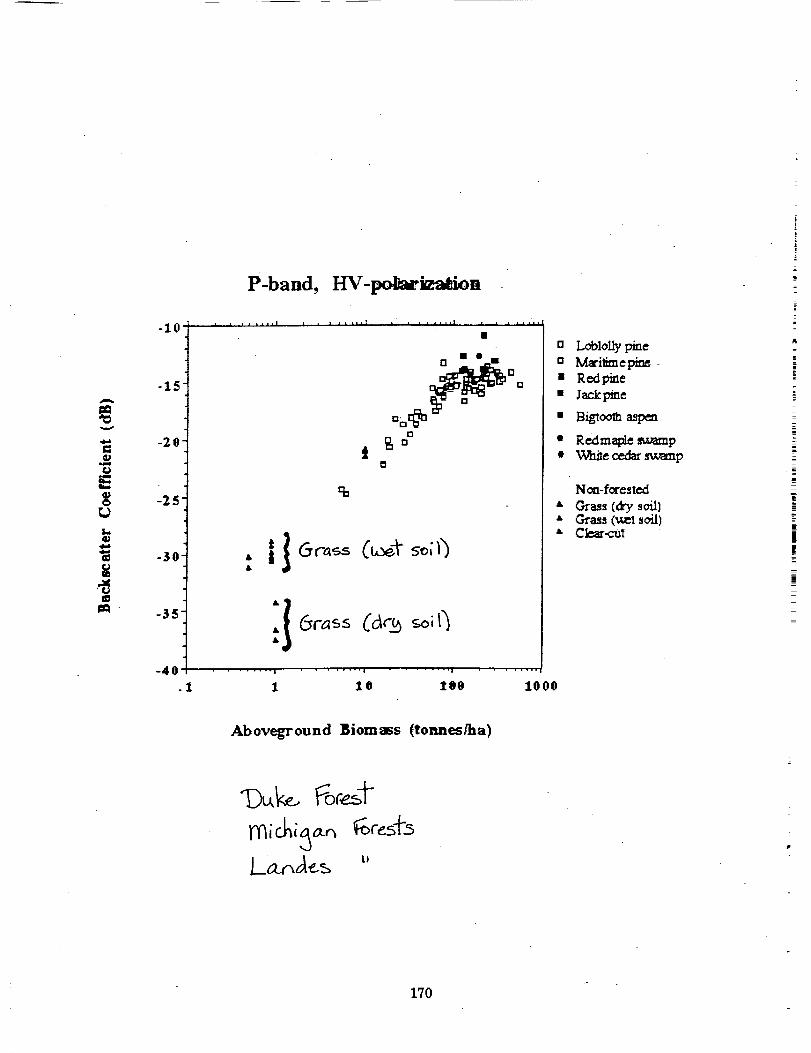
P-band, HV-potm-_n

] ] LJ LiJt[ i l I f , i . • ] t 1 i , ll,ll ___ I I [ i , i I •

• • "[] m

t0

: l 1 6r_ C_t so;_5

"l: @rass Car_ _oil]

-4_ ...... , ....... , ....... , .......• 1 1 1 0 _80 1000

tl

0

Loblolly pineM_itime_Re_ipine

Jac..kpine

Biglooth

Rexlmal:tle sv,_mpWhite cedar s',_mp

Non-forested

Grass (_T soil)Grass ('_i soil)Ckmr-cut

=

__=

_=

I

=It

!=mt

Aboveground ]_iomass (tonnestha)

170

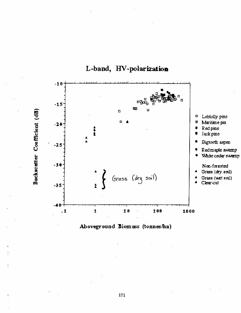
L-band, HV-polarization

v

4_

=wlml

g2

EO

11

4_

U

-10

-15'

-20

_25 ¸

-35'

-35

-40

.1

I I j , ,,,,I _ , , • l i i i i I ] i 1 i iiiii i j i i i i i i

t&

t

...... I

1

[] J

...... I ...... I

10 "tO0

u LobloUy pine

= Maritime pin

• Red pine

=- Jack pine

• B_:_la aspen

"- Redm_l¢ _,r_mp

• Vdhile ced_ s'a,_mp

Non-forested

" Grass (dry soil)

• Gra_s ('o_t soil)• Cle_r-cut

Aboveground Biomsss (tonnes/ha)

- 171

,_ MRS-20

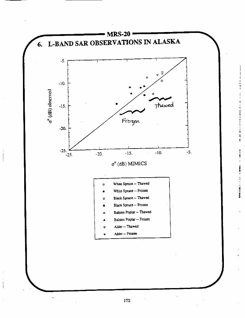
6. L-BAND SAIl OBSERVATIONS IN ALASKA

?,

O

m

oU

-5._ .... , .... l .... ' ....

.10._

-15.

-20.

-25.-25. -20. -15. -10.

G° (dB) MIMICS

e White Spruce -- Thawed

• White SlXUee - Frozen

t_ Black Spruce - Thawed

• Black Spruce -- Frozen

,,, Balsam poplar - Thawed

• Balsam Poplar -- Frozen

v Alder -- Thawed

• Alder - Froz_

-5.

172

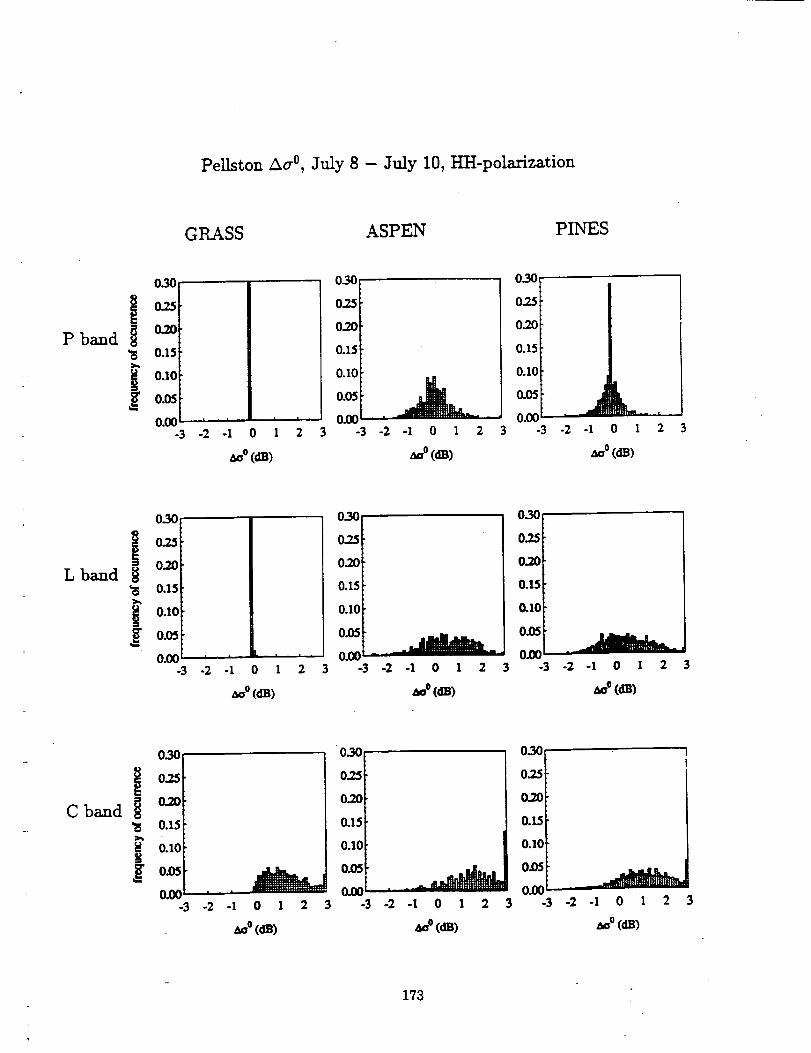
Pellston Aa °, July 8 - July 10, HI-I-polarization

GRASS ASPEN PINES

P band

0.30

0.2O

0.15

o,ot=I

-3 -2 -1 O 1 2 3

_o(¢IB)

0.301

_o(¢m)

0-_0_

O.25[-

o.15_-

0.10[-

o.05_

0.00 _ ,-3 -2 -1 O I 2 3

_°(dB)

L band

I

0.2O

0.15

o,of0.05[

t i • "

-3 -2 -1 O 1 2 3

_(dB)

0.30, O.._OI

0.251

0.201

0.151

O.IOI

0.051

OIIO '-3 -2 -1 O 1 2 3

Aoe(_)

C band

O30

0.15

0.10,

O.O0-3 -2 -1 O 1 2 3

_(_)

0.3O

O25

O.2O

0.15

O.IO

o_ _O.I_ ' "_

-3 -2 -I O 1 2 3

_o (cm)

O.3O

025

O,20

0.15

O.IO

o_ _0.0(3 ,

-3 -2 -1 0 1 2 3

173

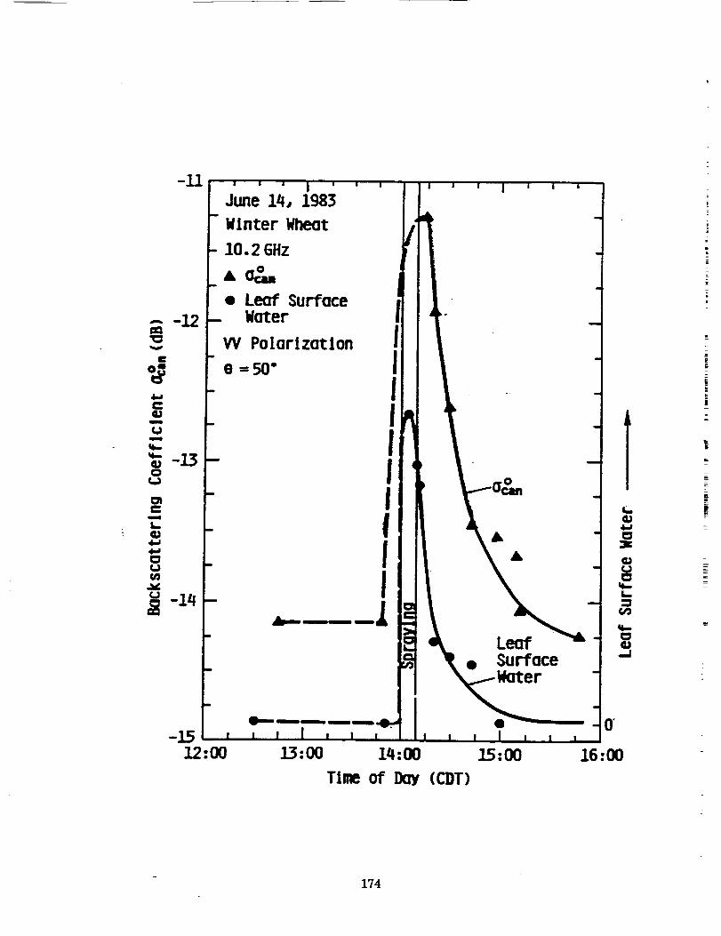
-11| | | | I i |

June 14. 1983

Winter Wheot

- 10.2 GHz

Ao&," • Leaf Surface

-12 - WoZer

_ e =.NI"

/8

-]5 , , , I , i ,--I]2:00

q

I,15:00 14:00

Time of Day (CDT)

LeafSurface

16:00

i

i

174

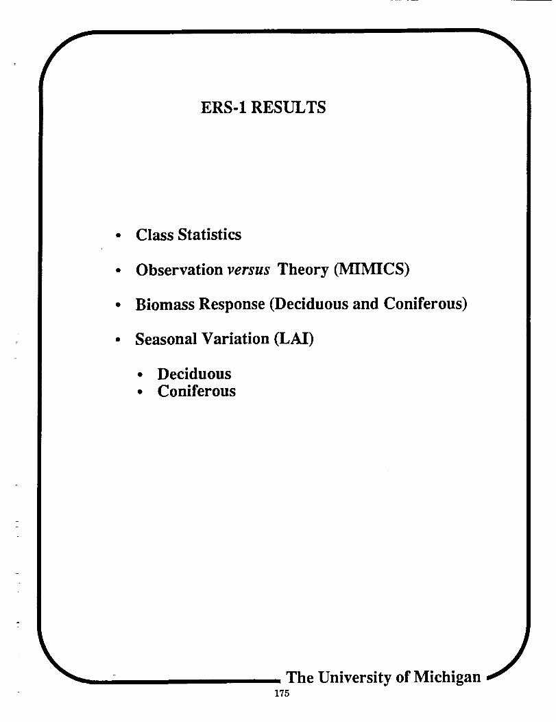
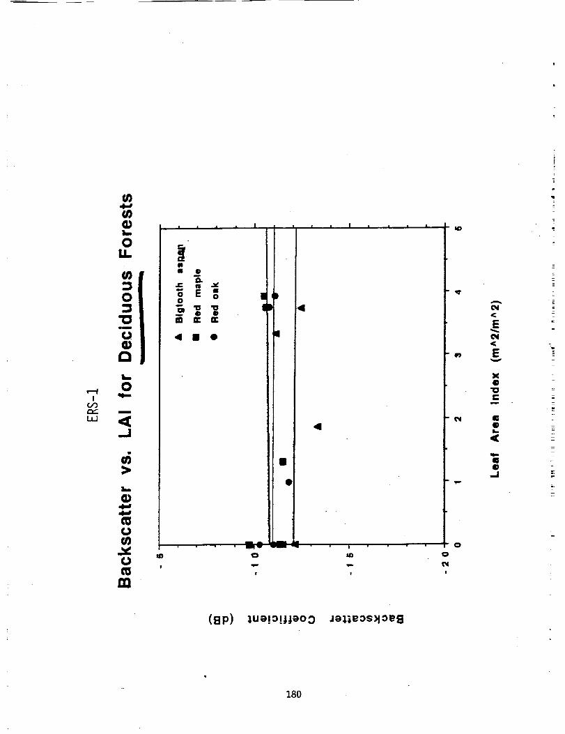
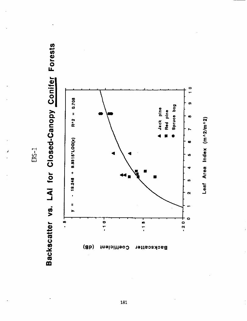
ERS-1 RESULTS

• Class Statistics

• Observation versus Theory (MIMICS)

• Biomass Response (Deciduous and Coniferous)

• Seasonal Variation (LAI)

• Deciduous• Coniferous

The University of Michigan J

175

ERS-1

0.35

ERS-1 Class Statistics for 3x3 Pixel Averages

0oo

-30.

InlandLakes Hay fields

Prairie

Concrete

LowlandConifers

Jack Pine NorthernHard woods

Red Pine

i

|

°

176

o_j

1,I

"0

0

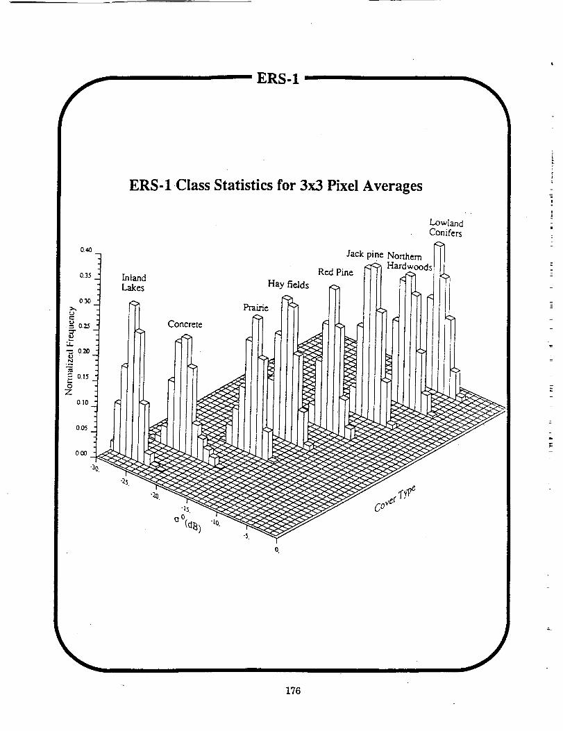
Comparison of SAlt Observations with MIMICS SimulationsC-band, W-polarization

A

0

1:1 line

Red pire

Jack pine

aeo n_eSugar mapleGrass

Lol_olty pine

Simulated Backscatter Coefficient (dB)

- 177

Q_

z 2,

""ro

rr

._ -_-

"0oQ)

m..,,n°v_

178

|

(n(n

oim

m

(n4)!.-

0LI.

"0C

0

0

::3

CDr_CCD

"0e,,4)Q.

1:3

I R i s

_D

0

I1

x

00

+

I!

!

r-

G)O.

01 (n0 _

°i_-_. __ _-_"_. o E o

_ o_

4 4. •

o

o

o

In

o

_- c3

o

o

o

o

In

i , i J o

0 m 0 In 0

•r- _ (_ (%1 toi ! | i !

(SP) ]ue!o!J;ooD Je]J, eosMoe_]

t_e-

e-f-0

Eo

C_

179

Ic_

i,i

U}

U_

oIL

U}

o

"0lamm

U4)

a

Ibm

o

.J

>

4)

4d

U

U!

z x ..L | |

_, o

E o..?

I_1 m E

• • •

!1 D

nl

IN

,my _

| !

<

E

<

E

X0

C

Q

qQ.J

i

!

z

E

=

z

(SP) Zue!o!_#eoo Je_,_eosHoeg

180

IGOCc_LI.J

0U.

mm

0(.3

>,,

|

0

0

0

_J

>

(D

m0

0mrn

II

|

(SP)

0 m 0

I im |

_ue!o!JJeoo 4ezleos)loe8

A

EC_<

Ev

X0

"0r"

m

W

L-

<

q_

J

- 181

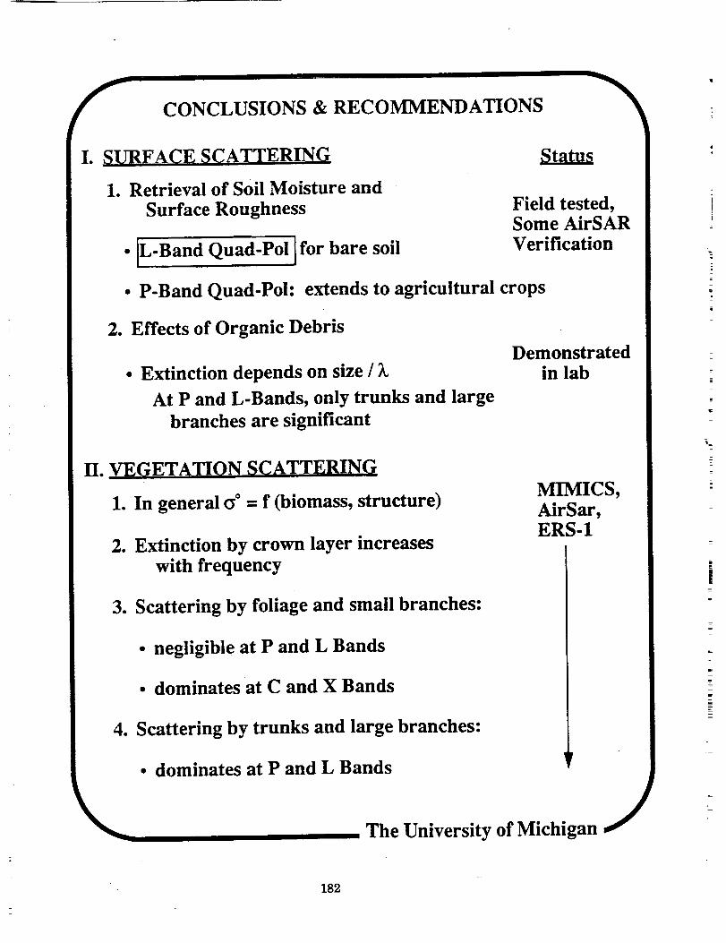
CONCLUSIONS & RECOMMENDATIONS

I. SURFACE SCATTERING Status

1. Retrieval of Soil Moisture andSurface Roughness

• IL.Band Quad-Pol i for bare soil

Field tested,Some AirSARVerification

• P-Band Quad-Pol: extends to agricultural crops

2. Effects of Organic Debris

• Extinction depends on size / _.

At P and L-Bands, only trunks and large

branches are significant

Demonstratedin lab

H. VEGETATION SCATTERING

1. In general o ° = f (biomass, structure)

2. Extinction by crown layer increaseswith frequency

3. Scattering by foliage and small branches:

• negligible at P and L Bands

• dominates at C and X Bands

MIMICS,AirSar,ERS-1

4. Scattering by trunks and large branches:

• dominates at P and L Bands

The University of Michigan J

182

CONCLUSIONS & RECOMMENDATIONS

i

• Even P-Band is insensitive to high biomassforests (Pacific NW _=_500 t0ns/ha)

6. Innundation under Forest Cover

L-Band HH I

7. Effects of Intercepted Precipitation

• negligible at P Band

• _=I dB increase or decrease at L-Band

• ---2 dB increase at C-Band

8. Freezing of Vegetation Leads to

Significant changes in _° at all Bands

SIR-BAirSARVerified

AirSAR,ScatteringVerified

AirSAR,MIMICSVerified

9. Deforestation Readily Detectable at

P and IL-Band[

SIR-B,AirSAR

10. LAI Foliar Biomass Estimation

[C-Band Quad or X-Band[

MIMICS,Field,AirSAR

11. Multi-Date Observations: Very Powerful Tool

• Requires good Relative Calibration (Stability) ___-+1 dB

• Requires good Absolute Calibration -=+ 1 dB

The University of Michigan J

183

!

p

i