RAD 229: MRI Signals - web. · PDF fileSection A1 B.Hargreaves - RAD 229 Lectures •75 min lectures -- Notes online at website •PDF, whole slide (print 4-6 per page) •Try to keep

RAD 229: MRI Signals and Sequences

Brian Hargreaves

All notes are on the course website

web.stanford.edu/class/rad229

B.Hargreaves - RAD 229Section A1

Course Goals

• Develop Intuition

• Understand MRI signals

• Exposure to numerous MRI sequences and naming:

• “gradient-echo”

• “spiral”

• “T2* BOLD”

• many, many confusing acronyms

• Expand EE369B, Complement EE369C, EE469B

2


General Course Logistics

• website: web.stanford.edu/class/rad229

• 3 Units, Letter or Cr/No Cr (EE300 Equivalent)

• Mon/Wed 1:30am-2:50pm

• CCSR 4107 (see calendar for changes)

• Texts (NOT required, but useful) • Bernstein M.

• Nishimura D.

3


Prerequisites / Grading

• Prerequisite: EE369B /equivalent

• (complements EE369C / EE469B)

• Paper / Matlab assignments / no MRI scanning

• Grading:

• 10% Attendance / Participation

• 10% Midterm

• 50% Homework + Project

• 30% Final

• Auditing:

• Please participate, but allow for-credit students to do so first

4


Homework / Project Options• Replace a HW Question:

• Spend <10min explaining how you’d do a question

• Replace it with a problem and solution that you choose, related to recent lectures

• Project: (details to follow)

• Approximately 1-2 Homeworks

• Simulate and present a sequence / signals / recon • A sequence we didn’t cover or simulate • A novel sequence that you devise • A sequence/recon with EE369C

5


Lectures

• 75 min lectures -- Notes online at website

• PDF, whole slide (print 4-6 per page)

• Try to keep numbered.

• Read ahead, but try not to ruin suspense(!)

• Please no email, texting etc in class

• I try to stay on time - please help by being on time

• Come early, I will try to entertain with questions etc!

• Class participation: questions, exercises

6


Homework

• Due Wednesday 11:59pm, (minus 10% per day late) • Paper:

• Lucas Center Rm P260 (under door)

• Frank Chavez (nearest cubicle)

• Electronically as PDF (encouraged): • Email w/ subject “RAD229: HW1” or similar, <10MB please!

• [email protected]

• Purpose is to learn the material. Note honor code • Please do not share solutions without permission

7


Other Information

• Instructor: Brian Hargreaves

• Office Hours - See Calendar

• Other Lecturers: Jennifer McNab, Others?

• No Teaching Assistant

• Web Site: web.stanford.edu/class/rad229

• Lecture notes, homework assignments, code

• Schedule / Room info, Announcements

8


Working Together - Rules

• Follow Honor Code

• Work together on homeworks,

• Discuss freely, but write your own matlab code

• Use resources, but not solutions

• No discussion of exams with others

• In general your responsibility is to learn!

• You should be able to explain anything you submit

9


Participation!

• FB: 1/10 (willing to answer, but not likely to be correct)

• ? (unlikely to answer but likely to be correct)

• Balance??!!

10


Introductions

• Your name?

• Who do you work with?

• Your Research?

• Comments - What you Hope to Learn?

11


Course Overview / Topics

• Review of Basic MRI (EE369B)

• Signal Calculation Tools, System Imperfections

• Pulse Sequences

• Advanced Acquisition Methods

• The RAD229 class will continue to evolve!

• Things might change, and your input will shape the course!

• You may know more than me about some topics

12


Background (~EE369B)

• “Magnetic Resonance Imaging” D. Nishimura

• Overview of NMR

• Hardware

• Image formation and k-space

• Excitation k-space

• Signals and contrast

• Signal-to-Noise Ratio (SNR)

• Pulse Sequences

13


MRI: Basic Concepts

14

Excitation Precession (Reception)

Relaxation (Recovery)

Static Magnetic Field (B0)

1H

N

S

Gradients (Relative Precession)

B0

B1

B0


Precession and Relaxation• Relaxation and precession are independent.

• Magnetization returns exponentially to equilibrium: • Longitudinal recovery time constant is T1 • Transverse decay time constant is T2

Precession Decay Recovery15


Magnetic Resonance Imaging (MRI)

• Polarization

• Excitation

• Signal Reception

• Relaxation

16


MRI Hardware

• Strong Static Field (B0) ~ 0.5-7.0T

• Radio-frequency (RF) field (B1) ~ 0.1uT

• Transmit, often built-in

• Receive, often many coils • Gradients (Gx, Gy, Gz) ~ 50-80 mT/m

17


B0: Static Magnetic Field• Goal: Strong AND Homogeneous magnetic field

• Typically 0.3 to 7.0 T

• Resonance prοportional to B0 : γ/2π = 42.58 MHz/T

• Superconducting magnetic fields - always on

• ~1000 turns, 700 A of current

• Passively shimmed by adjusting coil locations

• The following increase with with B0:

• Polarization, Larmor Frequency, Spectral separation, T1

• RF power for given B1

• B0 variations due to susceptibility, chemical shift18


B0: The “Rotating” Coordinate Frame

• Usually demodulate by Larmor frequency to “baseband” • Also called the rotating frame

19


B1+: RF Transmit Field• Goal: Homogeneous rotating magnetic field

• Typically up to about 25 uT (Amplifier, SAR limits)

• Requires varying power based on subject size

• Dielectric effects cause B1+ variations at higher B0

• Amplifier power: kW to tens of kW

• Specific Absorption Rate (SAR) Limits:

• Power proportional to B02 and B12

• Goal is to limit heating to <1∘C

20


B1-: RF Receive

• Goal: High sensitivity, spatially limited, low noise

• “Birdcage” coils

• Uniform B1- but single channel

• Surface coils

• Varying B1- but high sensitivity

• Coil arrays

• Multiple channels with Varying B1-

• Allows some spatial localization: Parallel Imaging

21


RF Coils

22


Receiver System

• 500 to 1000 k samples/s

• Complex sampling

• Low-pass filter capability

• Typically 32-128 channels

• Time-varying frequency and phase modulation (Typically single-channel)

23


Gradients

• Goal: Strong, switchable, linear Bz variation with x,y,z

• Peak amplitude ~ 50-80 mT/m (~ 200A)

• Switching 200 mT/m/ms (~1500 V)

• Limits:

• Amplifier power, heating, coil heating

• “dB/dt” limitation due to peripheral nerve stimulation

• Switching induces Eddy Currents

• Concomitant terms (Bx and By variations)

• Non-linearities (often correctable)24


Gradient Waveforms

• Mapping of position to frequency, slope = γG

• Typically waveforms are trapezoidal

• Constant amplitude and slew-rate limits

25

Position

Frequency �Gread

Time

Amplitude


Shims

• Goal usually to make B0 more uniform with subject

• Center frequency

• Linear shims (Up to ~1% offset to gradients)

• Higher-order (HO) shims (Spherical Harmonics)

• Shim arrays, Shim+RF (Current Research)

• Usually HO shims not dynamically switchable

26


Review Questions• Which field is the “receive” field?

• B1-

• Which field is always on?

• B0

• What receive bandwidth corresponds to 500,000 samples/second?

• ±250 kHz

• Why might small surface coils (or arrays) be useful?

• High sensitivity, Low noise, Spatially limiting

27


Image Formation and k-space

• Gradients and phase

• Signal equation

• Sampling / Aliasing

• Parallel Imaging

• Many reconstruction methods in EE369C

28


x

x

x

Gradient Strength and Sign

Can control both amplitude and duration

Positive Gradient

Negative Gradient

Double StrengthHalf-Duration

29


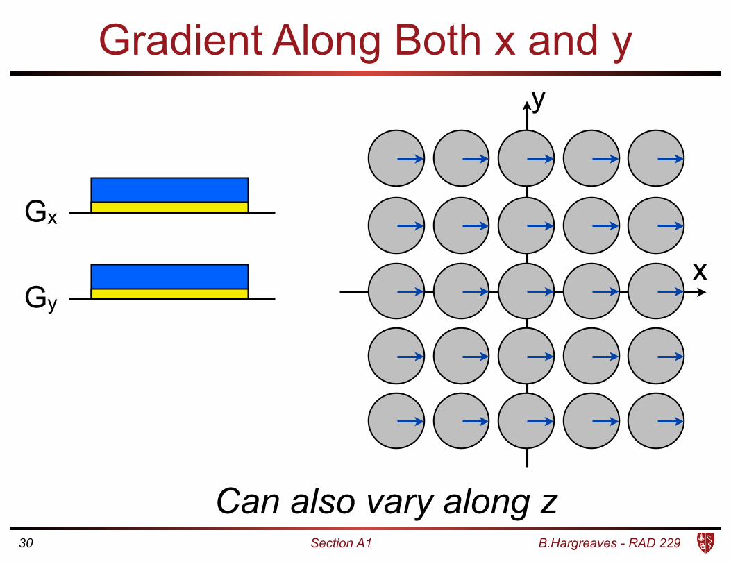
Gradient Along Both x and y

Gx

Gyx

y

Can also vary along z30


Ribbon Analogy

• Gradients induce “phase twist”

• Twist has a number of cycles and a “sign”

• Twist can be along any direction

x

31


Gradients and Phase• Control gradient amplitude and duration

• Can control frequency:

Frequency = γ(Gx x + Gy y)

• Can “encode” phase over duration t Angle = γt (Gx x + Gy y + Gz z)

• Generally:

� = �(xZ

G

x

dt + y

ZG

y

dt)

32

� = �(xZ

G

x

dt + y

ZG

y

dt)

What are the units of Frequency and Angle (φ) here?


Signal Equations

• For a single spin:

• Represent as exponential:

• Sum over many spins:

• Signal equation:

33

� = �(xZ

G

x

dt + y

ZG

y

dt)

kx,y

(t) =�

2⇡

Zt

0G

x,y

(⌧)d⌧

s(t) = FT [⇢(x, y)]|kx

(t),ky

(t)

s = e�i�(xRG

x

dt+y

RG

y

dt)

s =

Z 1

�1

Z 1

�1⇢(x, y)e�i�(x

RG

x

dt+y

RG

y

dt)dxdy

s =

Z 1

�1

Z 1

�1⇢(x, y)e�2⇡i(k

x

x+k

y

y)dxdy


Fourier Transform in MRI

• Given M(k) at enough k locations, we can find ρ(r)

• It does not matter how we got to k!

M(k) ρ(r)Fourier

Transform

34

s(t) = FT [⇢(x, y)]|kx

(t),ky

(t)

What are the units of kx(t) and ky(t) ?


Fourier Encoding and Reconstruction

k-space

ky

kx

Gradient-induced Phase

x

k-space

ky

kx xSum over k-space

Sum over image

35

Spatial Harmonic

Encoding

Reconstruction


k-space: Spatial Frequency Map

ky

kx

36

k-space

In terms of pixel-width, what is the width of k-space?


Image Formation and SamplingReadout Gradient

time

Phase-Encode Gradient

time

k-space

kphase

kread

Readout Direction

37


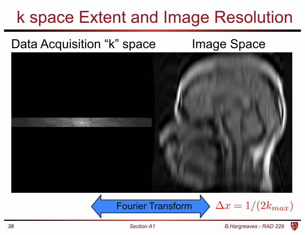
k space Extent and Image ResolutionData Acquisition “k” space Image Space

Fourier Transform

38

�x = 1/(2kmax

)


Sampling and Field of View• Sampling density determines FOV • Sparse sampling results in aliasing

Rea

dout

Phase-Encode

kphase

kread

kphase

kread

FOV FOV

39

FOV = 1/�ky


Phase-Encoding with Two Coils

kx

ky

k-space kx

ky

kx

ky

40


Readout Parameters• Bandwidth linked to readout

• “half-bandwidth” (GE) = 0.5 x sample rate

• Same as Filter bandwidth (baseband)

• Pixel-bandwidth often useful

41

Position

Frequency

Full BandwidthBandwidth per Pixel

FOV

Pixel

�Gread

BW

pix

= �G

read

�x

BWhalf = �GreadFOV/2


Imaging Example

• Desired Image Parameters:

• 256 x 256, over 25cm FOV

• (±)125 kHz bandwidth

• What are the...

• Sampling period?

• Readout duration?

• Gradient strength?

• Bandwidth per pixel?

• k-space extent?

42

• 1/(2*125kHz) = 4µs

• 4µs * 256 = 1ms

• 250kHz / 0.25m / 42.58kHz/mT

• 23 mT/m (2.3 G/cm)

• 250kHz/256 pix = ~ 1kHz/pixel

• 0.5 / 1mm = 0.5 mm-1 = 5cm-1


2D Multislice vs 3D Slab Imaging

• Shorter scan times, reduced motion artifact

• Continuous coverage

• Thinner slices, reformats

2D 3D

43


Imaging Summary

• Gradients impose time-varying linear phase

• k-space is time-integral of gradients

• k-space samples Fourier Transform to/from image

• Density of k-space <> FOV (image extent)

• Extent of k-space <> Resolution (image density)

• 3D k-space is possible

• Parallel imaging uses coils to extend FOV

44


Excitation

• General principles of excitation

• Selective Excitation with gradients

• Relationships for slice excitation


• Much more covered in EE469B

45


Excitation: B1 Field

• Direction of B1 is perpendicular to B0

• Magnetization precesses about B1

• Turn on and off B1 to “tip” magnetization

• Problem: We can’t turn off B0!

• Precession still around B0

46


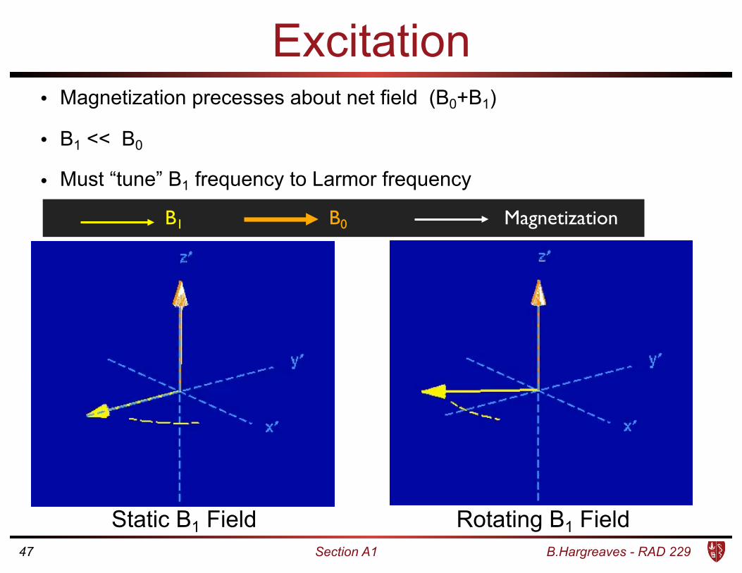
Excitation

B1 MagnetizationB0

• Magnetization precesses about net field (B0+B1) • B1 << B0 • Must “tune” B1 frequency to Larmor frequency

Static B1 Field Rotating B1 Field47


Excitation: Rotating Frame• “Excite” spins out of their equilibrium state. • B1 << B0 • Transverse RF field (B1) rotates at γB0 about z-axis.

B1 MagnetizationB0

Rotating Frame, “On resonance”Static Frame48


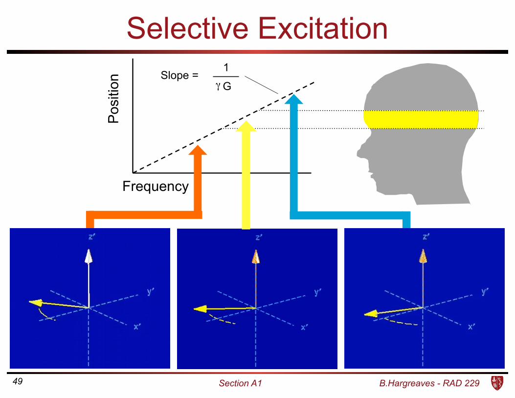
Selective Excitation

Pos

ition

Slope = 1

γ G

Frequency

49


Selective Excitation

B1 Frequency

Mag

nitu

de

Time

RF

Am

plitu

de

Pos

ition Slope = 1

γ G

Larmor Frequency

+

+=

50

Slice width = BWRF / γGz

Slice center = Frequency / γGz


Excitation Example

• Given a 2 kHz RF pulse bandwidth, and desired

• 5mm thick slice

• Slices at -2cm, 0, 2cm

• What are the...

• Gradient strength? (γ/2π)Gz

• Excitation frequencies?

• Thinnest slice possible with 50mT/m max gradients?

51

• 2kHz/5mm = 400kHz/m ~ 9.4 mT/m (0.94 G/cm)

• BW/slice = 2kHz/5mm, so -8, 0, 8 kHz

• (9.4/50)*5mm ~1mm slice


Excitation k-Space

• Excitation k-space goes backwards from end of RF/gradient pair:

• Excited profile = Fourier Transform of excitation k-space

• Central flip angle = area under pulse (may be zero!):

52

ke(t) = � �

2⇡

Z T

tG(⌧)d⌧ kr(t) =

�

2⇡

Z t

0G(⌧)d⌧

↵ = �

ZB1(⌧)d⌧


Excitation Example

• For a 1ms, constant RF pulse of amplitude 10µT …

• What is the flip angle?

• How does RF energy change if the duration is halved and amplitude doubled?

53

• (42.58 kHz/mT)(0.01mT)(1ms) = 0.4258 cycles = 153º

• Doubles - (2A)2(T/2) = 2(A2T)


Signals and Contrast• Simple Bloch Equation Solutions

• Basic contrast mechanisms: T1, T2, IR, Steady-State

54

T2-Weighted T2-w FLAIR T1-w FLAIR

Gradient Echo Diffusion-Weighted Apparent Diffusion Coefficient (ADC)


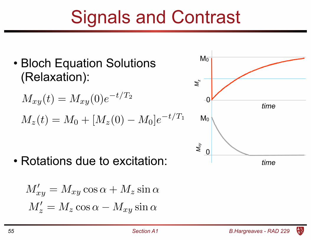
Signals and Contrast

• Bloch Equation Solutions (Relaxation):

• Rotations due to excitation:

55

Mxy

(t) = Mxy

(0)e�t/T2

Mz(t) = M0 + [Mz(0)�M0]e�t/T1

M 0xy

= Mxy

cos↵+Mz

sin↵

M 0z

= Mz

cos↵�Mxy

sin↵M

xy

M0

0

Mz

M0

0

time

time


Echo Time (TE): T2 weighting

RF

Sig

nal

90º 90º

1

0

Mz

Short TELong TE

56

TE = Time from RF to “echo”


T2 Contrast

Dardzinski BJ, et al. Radiology, 205: 546-550, 1997.

Signal

Echo Time (ms)

TE = 20

TE = 40

TE = 60

TE = 80

57


Repetition Time (TR) : T1 Weighting

Each excitation starts with reduced Mz

RF

Sig

nal

90º 90º

1

0

Mz

90º

Mz

Mxy

58


T1-Weighted Spin Echo

Sig

nal

Time

Sig

nal

Time

Short Repetition Long Repetition

Joint Fluid

Bone

59


Short TR Long TR

Short TE

Incomplete Recovery Minimal Decay T1 Weighting

Full Recovery Minimal Decay Proton Density Weighting

Long TE

Incomplete Recovery Signal Decay Mixed Contrast (Not used much)

Full Recovery Signal Decay T2 Weighting

Basic Contrast Question (TE, TR)

60 Images Courtesy of Anne Sawyer


Inversion-Recovery

180º 180º

RF

Sig

nal

1

-1

0

• Fat suppression based on T1

• Short TI Inversion Recovery (STIR)

TI

61


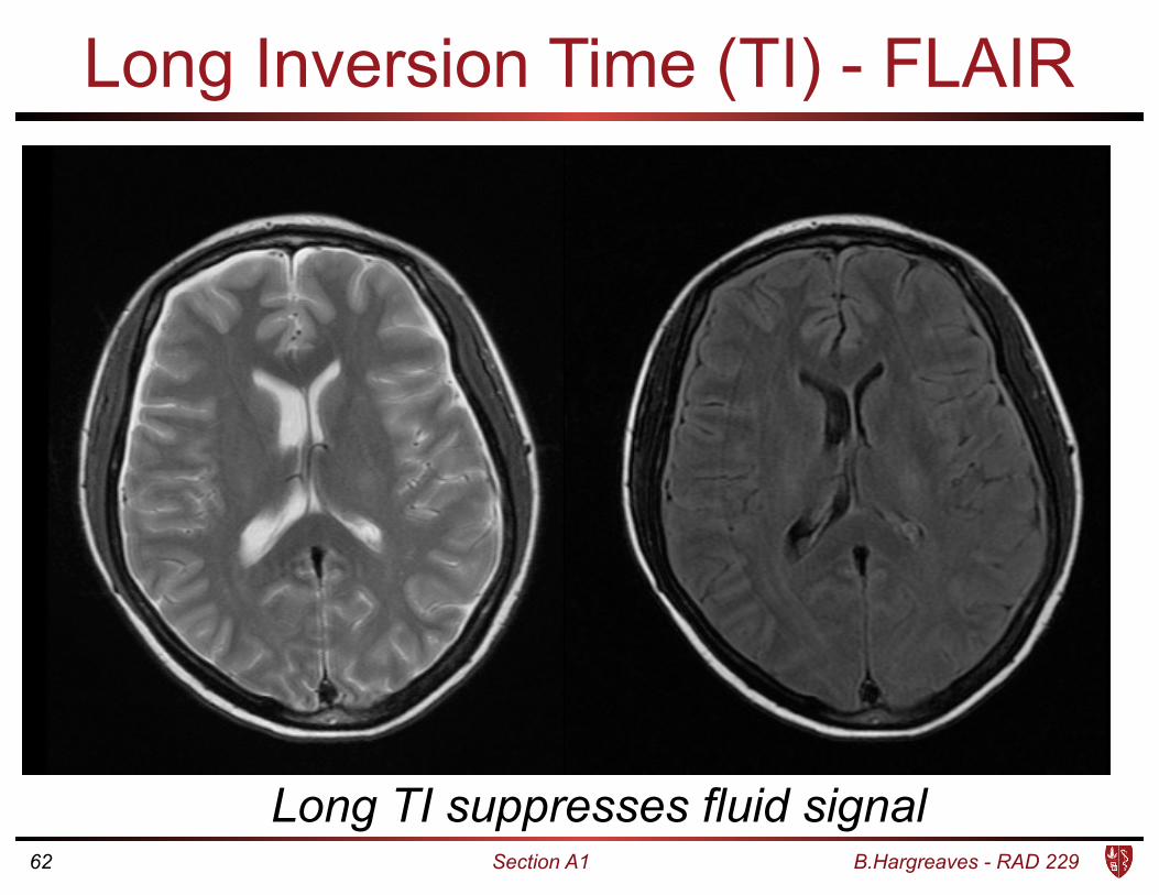
Long Inversion Time (TI) - FLAIR

Long TI suppresses fluid signal62


Signal Question

• Inversion Recovery Sequence: • TR = 1s, TI = 0.5s, TE=50ms

• What is the signal for T1=0.5s, T2=100ms?

63

180º 180º

RF

TI

TE

TR

90º

• Signal (Mxy) decays to 0 • Mz does not fully recover • exp(-1) = 037 • Mz is 0.63 M0 before 180º

• At TI, Mz-M0 = 1.63 exp(-1) • Mz ~ 0.4 M0 • T2 decay ~ exp(-0.5) ~ 0.6 • Signal = 0.4 x 0.6 = 0.24 M0


Steady-State Sequences

• Repeated sequences always lead to a “steady state”

• Sometimes includes equilibrium (easier)

• Otherwise trace magnetization and solve equations

• Example: Small-tip, TE=0

64

Mz(TR) = M0 + [Mz(TE)�M0]e�TR/T1

Mz(TE) = Mz(TR) cos↵

Combining...

...“TR” “TE”

Mz(TR) = M01� e�TR/T1

1� e�TR/T1cos↵


Summary ~ Background I

• Overview of NMR

• Hardware

• Image formation and k-space


• Signals and contrast

65

Documents

RAD 229: MRI Signals - web. · PDF fileSection A1 B.Hargreaves - RAD 229 Lectures •75 min lectures -- Notes online at website •PDF, whole slide (print 4-6 per page) •Try to keep