RAD 229: MRI Signals - Stanford Universityweb.stanford.edu/class/rad229/Notes/0-BasicMR-Review.pdf · B.Hargreaves - RAD 229 Lectures • 75 min lectures -- Notes online at website

RAD 229: MRI Signals and Sequences

Brian Hargreaves

• All notes are on the course website

• web.stanford.edu/class/rad229

B.Hargreaves - RAD 229

Course Goals

• Develop Intuition

• Understand MRI signals

• Exposure to numerous MRI sequences

• Expand EE369B, Complement EE369C, EE469B

2


General Course Logistics

• website: web.stanford.edu/class/rad229

• 3 Units, Letter or Credit/No Credit

• Mon/Wed 11:00am-12:15pm

• M106 and M114 (see web)

• Texts (optional but useful)• Bernstein M.

• Nishimura D.

3


Prerequisites / Grading• Prerequisite: EE369B /equivalent

• (complements EE369C / EE469B)

• Paper / Matlab assignments / no MRI scanning

• Grading:

• 10% Attendance / Participation

• 15% Midterm

• 40% Homework

• 35% Final

• Auditing:

• Please participate, but allow for-credit students to do so first

4


Lectures

• 75 min lectures -- Notes online at website

• PDF, whole slide (print 4-6 per page)

• Try to keep numbered.

• Read ahead, but try not to ruin suspense(!)

• Please no email, texting etc in class

• I try to stay on time - please help by being on time

• Come early, I will try to entertain with questions etc!

• Class participation: questions, exercises

5


Homework

• Due Wednesday 5pm, (minus 10% per day late)

• Paper:• Lucas Center Rm P260 (under door)

• Kristin Zumwalt (nearest cubicle)

• Electronically as PDF (encouraged):• Email w/ subject “RAD229: HW1” or similar, <10MB please!

• [email protected]

• Purpose is to learn the material. Note honor code

6


Other Information• Instructor: Brian Hargreaves

• Other Lecturers: Jennifer McNab, Others?

• Teaching Assistant: Ethan Johnson ([email protected])

• HW assistance

• Office hours

• Web Site: web.stanford.edu/class/rad229

• Lecture notes, homework assignments, code

• Schedule / Room info, Announcements7


Working Together - Rules

• Follow Honor Code

• Work together on homeworks,

• Discuss freely, but write your own matlab code

• Use resources, but not solutions

• No discussion of exams with others

• In general your responsibility is to learn!

• You should be able to explain anything you submit

8


Introductions

• Your name?

• Who do you work with?

• What do you work on?

• What do you hope to learn here?

9


Course Overview / Topics• Review of Basic MRI (EE369B)

• Signal Calculation Tools

• System Imperfections

• Sequences I: (Spin Echo and Gradient Echo)

• Sequences II: (Rapid, Quantitative, Mag Prep)

• Congratulations on being the first RAD229 class...!

• Things might change, and your input will shape the course!

• You may know more than me about some topics

• Prize for most useful feedback on course lectures/notes

10


Review of EE369B

• “Magnetic Resonance Imaging” D. Nishimura

• Overview of NMR

• Hardware

• Image formation and k-space

• Excitation k-space

• Signals and contrast

• Signal-to-Noise Ratio (SNR)

• Pulse Sequences

11


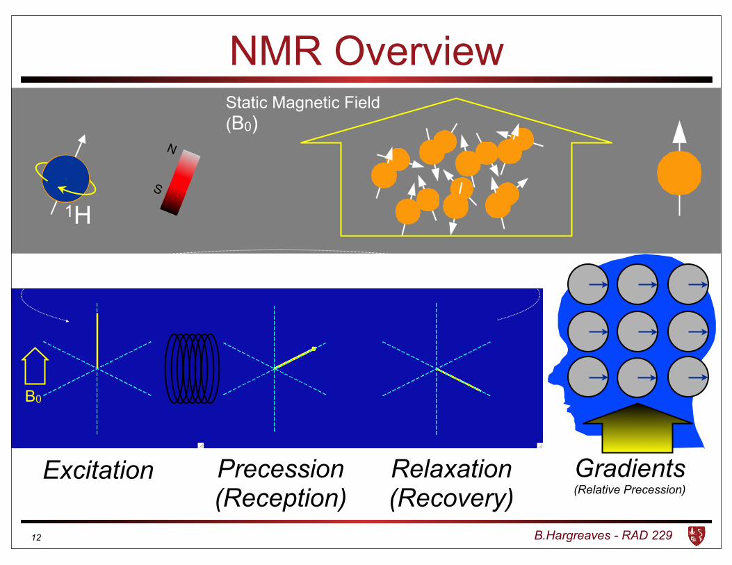
NMR Overview

Excitation Precession(Reception)

Relaxation(Recovery)

Gradients(Relative Precession)

B0

12

Static Magnetic Field (B0)

1H

N

S


Precession and Relaxation• Relaxation and precession are independent.

• Magnetization returns exponentially to equilibrium:• Longitudinal recovery time constant is T1

• Transverse decay time constant is T2

Precession Decay Recovery13


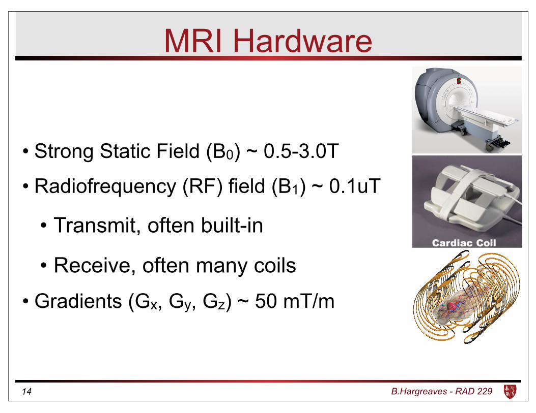
MRI Hardware

• Strong Static Field (B0) ~ 0.5-3.0T

• Radiofrequency (RF) field (B1) ~ 0.1uT

• Transmit, often built-in

• Receive, often many coils

• Gradients (Gx, Gy, Gz) ~ 50 mT/m

14


B0: Static Magnetic Field• Goal: Strong AND Homogeneous magnetic field

• Typically 0.3 to 3.0 T

• Resonance prοportional to B0 : γ/2π = 42.58 MHz/T

• Superconducting magnetic fields - always on

• ~1000 turns, 700 A of current

• Passively shimmed by adjusting coils

• The following increase with with B0:

• Polarization, Larmor Frequency, Spectral separation, T1

• RF power for given B1

• B0 variations due to susceptibility, chemical shift

15


B0: The “Rotating” Coordinate Frame

• Usually demodulate by Larmor frequency to “baseband”• Also called the rotating frame

16


B1+: RF Transmit Field

• Goal: Homogeneous rotating magnetic field

• Typically up to about 25 uT (Amplifier, SAR limits)

• Requires varying power based on subject size

• Dielectric effects cause B1+ variations at higher B0

• Amplifier power on the order of kW

• Specific Absorption Rate (SAR) Limits:

• Power proportional to B02 and B12

• Goal is to limit heating to <1∘C

17


B1-: RF Receive

• Goal: High sensitivity, spatially limited, low noise

• “Birdcage” coils

• Uniform B1- but single channel

• Surface coils

• Varying B1- but high sensitivity

• Coil arrays

• Multiple channels with Varying B1-

• Allows some spatial localization: Parallel Imaging

18


RF Coils

19


Receiver System

• 500 to 1000 k samples/s

• Complex sampling

• Low-pass filter capability

• Typically 32-128 channels

• Time-varying frequency and phase modulation (Typically single-channel)

20


Gradients• Goal: Strong, switchable, linear Bz variation with x,y,z

• Peak amplitude ~ 50 mT/m (~ 200A)

• Switching 200 mT/m/ms (~1500 V)

• Limits:

• Amplifier power, heating, coil heating

• “dB/dt” limitation due to peripheral nerve stimulation

• Switching induces Eddy Currents

• Concomitant terms (Bx and By variations)

• Non-linearities (often correctable)21


Gradient Waveforms

• Mapping of position to frequency, slope = γG

• Typically waveforms are trapezoidal

• Constant amplitude and slew-rate limits

22

Position

Frequency �Gread

Time

Amplitude


Image Formation and k-space

• Gradients and phase

• Signal equation

• Sampling / Aliasing

• Parallel Imaging

• Many reconstruction methods in EE369C

23


x

x

x

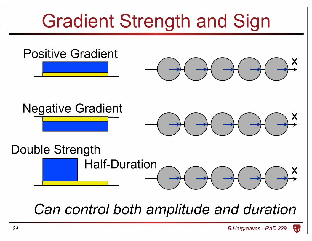
Gradient Strength and Sign

Can control both amplitude and duration

Positive Gradient

Negative Gradient

Double StrengthHalf-Duration

24


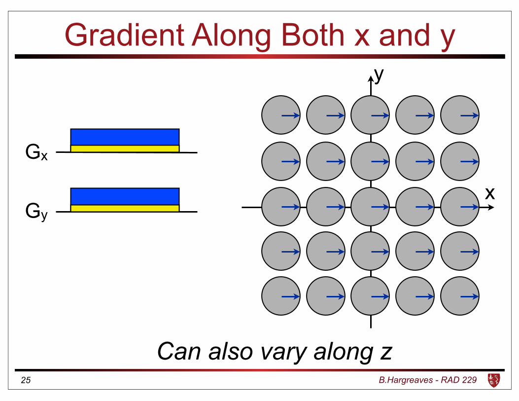
Gradient Along Both x and y

Gx

Gyx

y

Can also vary along z25


Ribbon Analogy

• Gradients induce “phase twist”

• Twist has a number of cycles and a “sign”

• Twist can be along any direction

x

26


Gradients and Phase

• Control gradient amplitude and duration

• Can control frequency:

Frequency = γ(Gx x + Gy y)

• Can “encode” phase over duration t

Angle = γt (Gx x + Gy y + Gz z) • Generally:

� = �(xZ

G

x

dt + y

ZG

y

dt)

27

� = �(xZ

G

x

dt + y

ZG

y

dt)


Signal Equations

• For a single spin:

• Represent as exponential:

• Sum over many spins:

• Signal equation:

28

� = �(xZ

G

x

dt + y

ZG

y

dt)

kx,y

(t) =�

2⇡

Zt

0G

x,y

(⌧)d⌧

s(t) = FT [⇢(x, y)]|kx

(t),ky

(t)

s = e�i�(xRG

x

dt+y

RG

y

dt)

s =

Z 1

�1

Z 1

�1⇢(x, y)e�i�(x

RG

x

dt+y

RG

y

dt)dxdy

s =

Z 1

�1

Z 1

�1⇢(x, y)e�i(k

x

x+k

y

y)dxdy


Fourier Transform in MRI

• Given M(k) at enough k locations, we can find ρ(r)

• It does not matter how we got to k!

M(k) ρ(r)Fourier

Transform

29

s(t) = FT [⇢(x, y)]|kx

(t),ky

(t)


Fourier Encoding and Reconstruction

k-space

ky

kx

Gradient-induced Phase

x

k-space

ky

kx xSum over k-space

Sum over image

30

Spatial Harmonic

Encoding

Reconstruction


k-space: Spatial Frequency Map

k-space

ky

kx

31


Image Formation and SamplingReadout Gradient

time

Phase-Encode Gradient

time

k-space

kphase

kread

Readout Direction

32


k space Extent and Image ResolutionData Acquisition “k” space Image Space

Fourier Transform

33

�x = 1/(2kmax

)


Sampling and Field of View• Sampling density determines FOV• Sparse sampling results in aliasing

Rea

dout

Phase-Encode

kphase

kread

kphase

kread

FOV FOV

34

FOV = 1/�ky


Phase-Encoding with Two Coils

kx

ky

k-space kx

ky

kx

ky

35


Readout Parameters• Bandwidth linked to readout

• “half-bandwidth” (GE) = 0.5 x sample rate

• Same as Filter bandwidth (baseband)

• Pixel-bandwidth often useful

36

Position

Frequency

Full BandwidthBandwidth per Pixel

FOV

Pixel

�Gread

BW

pix

= �G

read

�x

BWhalf = �GreadFOV/2


Imaging Example• Desired Image Parameters:

• 256 x 256, over 25cm FOV

• 125 kHz bandwidth

• What are the...

• Readout duration?

• Sampling period?

• Gradient strength?

• Bandwidth per pixel?

• k-space extent?

37


2D Multislice vs 3D Slab Imaging

• Shorter scan times, reduced motion artifact

• Continuous coverage

• Thinner slices, reformats

2D 3D

38


Imaging Summary

• Gradients impose time-varying linear phase

• k-space is time-integral of gradients

• k-space samples Fourier Transform to/from image

• Density of k-space <> FOV (image extent)

• Extent of k-space <> Resolution (image density)

• 3D k-space is possible

• Parallel imaging uses coils to extend FOV

39


Excitation

• General principles of excitation

• Selective Excitation with gradients

• Relationships for slice excitation


• Much more covered in EE469B

40


Excitation: B1 Field

• Direction of B1 is perpendicular to B0

• Magnetization precesses about B1

• Turn on and off B1 to “tip” magnetization

• Problem: We can’t turn off B0!

• Precession still around B0

41


Excitation

B1 MagnetizationB0

• Magnetization precesses about net field (B0+B1)

• B1 << B0

• Must “tune” B1 frequency to Larmor frequency

Static B1 Field Rotating B1 Field42


Excitation: Rotating Frame• “Excite” spins out of their equilibrium state.• B1 << B0

• Transverse RF field (B1) rotates at γB0 about z-axis.

B1 MagnetizationB0

Rotating Frame, “On resonance”Static Frame43


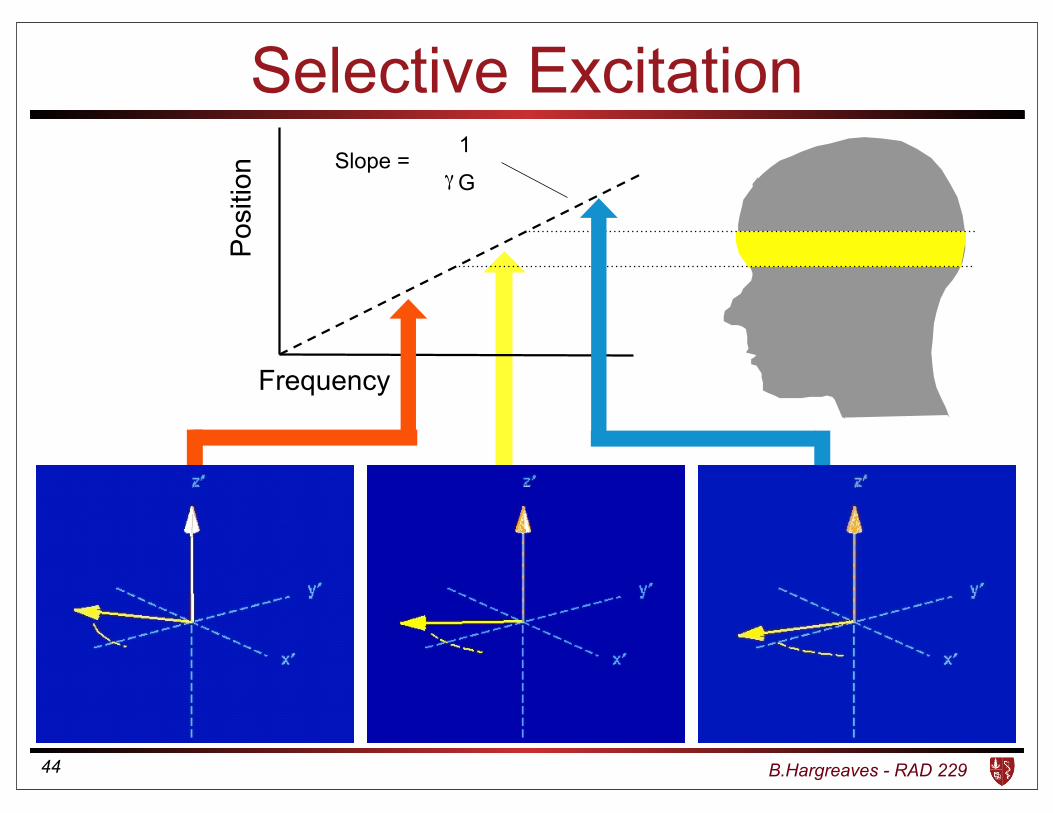
Selective Excitation

Pos

ition

Slope = 1

γ G

Frequency

44


Selective Excitation

B1 Frequency

Mag

nitu

de

Time

RF

Am

plitu

de

Pos

ition Slope = 1

γ G

Larmor Frequency

+

+=

45

Slice width = BWRF / γGz

Slice center = Frequency / γGz


Excitation Example

• Given a 2 kHz RF pulse bandwidth, and desired

• 5mm thick slice

• Slices at -2cm, 0, 2cm

• What are the...

• Gradient strength?

• Excitation frequencies?

46


Excitation k-Space

• Excitation k-space goes backwards from end of RF/gradient pair:

• Excited profile = Fourier Transform of excitation k-space

• Central flip angle = area under pulse (may be zero!):

47

ke(t) = � �

2⇡

Z T

tG(⌧)d⌧ kr(t) =

�

2⇡

Z t

0G(⌧)d⌧

↵ = �

ZB1(⌧)d⌧


Signals and Contrast

• Simple Bloch Equation Solutions

• Basic contrast mechanisms: T1, T2, IR, Steady-State

48


Signals and Contrast

• Bloch Equation Solutions (Relaxation):

• Rotations due to excitation (ignoring transverse M before excitation):

49

Mxy

(t) = Mxy

(0)e�t/T2

Mz(t) = M0 + [Mz(0)�M0]e�t/T1

M 0xy

= Mxy

cos↵+Mz

sin↵

M 0z

= Mz

cos↵�Mxy

sin↵


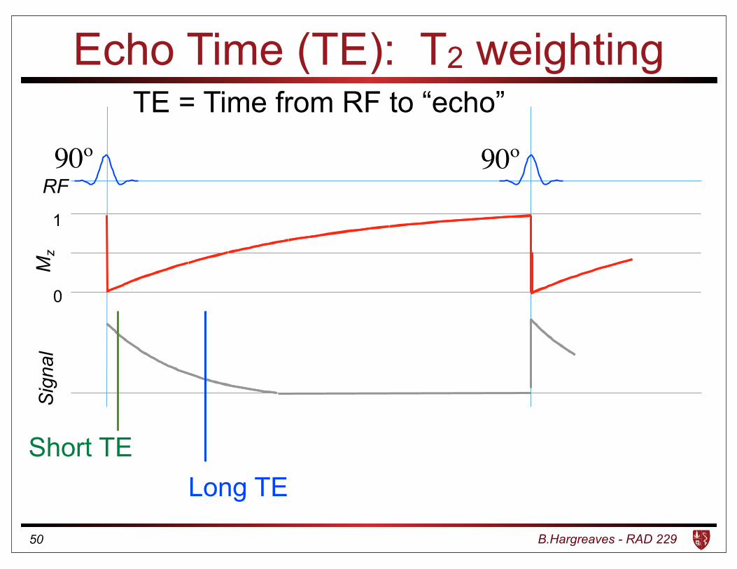
Echo Time (TE): T2 weighting

RF

Sig

nal

90º 90º

1

0

Mz

Short TELong TE

50

TE = Time from RF to “echo”


T2 Contrast

Dardzinski BJ, et al. Radiology, 205: 546-550, 1997.

Signal

Echo Time (ms)

TE = 20

TE = 40

TE = 60

TE = 80

51


Proton-Density and T2-weighted Contrast

Proton Density Weighted T2 Weighted

52


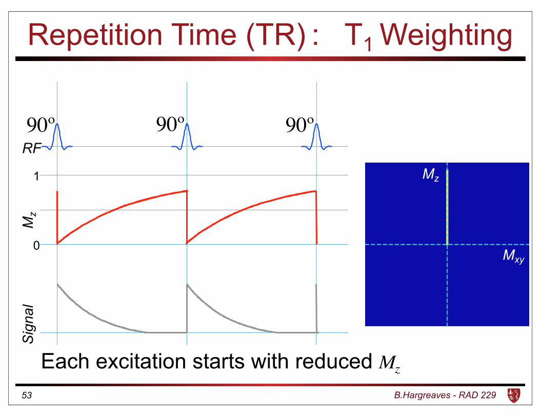
Repetition Time (TR) : T1 Weighting

Each excitation starts with reduced Mz

RF

Sig

nal

90º 90º

1

0

Mz

90º

Mz

Mxy

53


T1 Weighted Spin Echo

Sig

nal

Time

Sig

nal

Time

Short Repetition Long Repetition

Joint Fluid

Bone

54


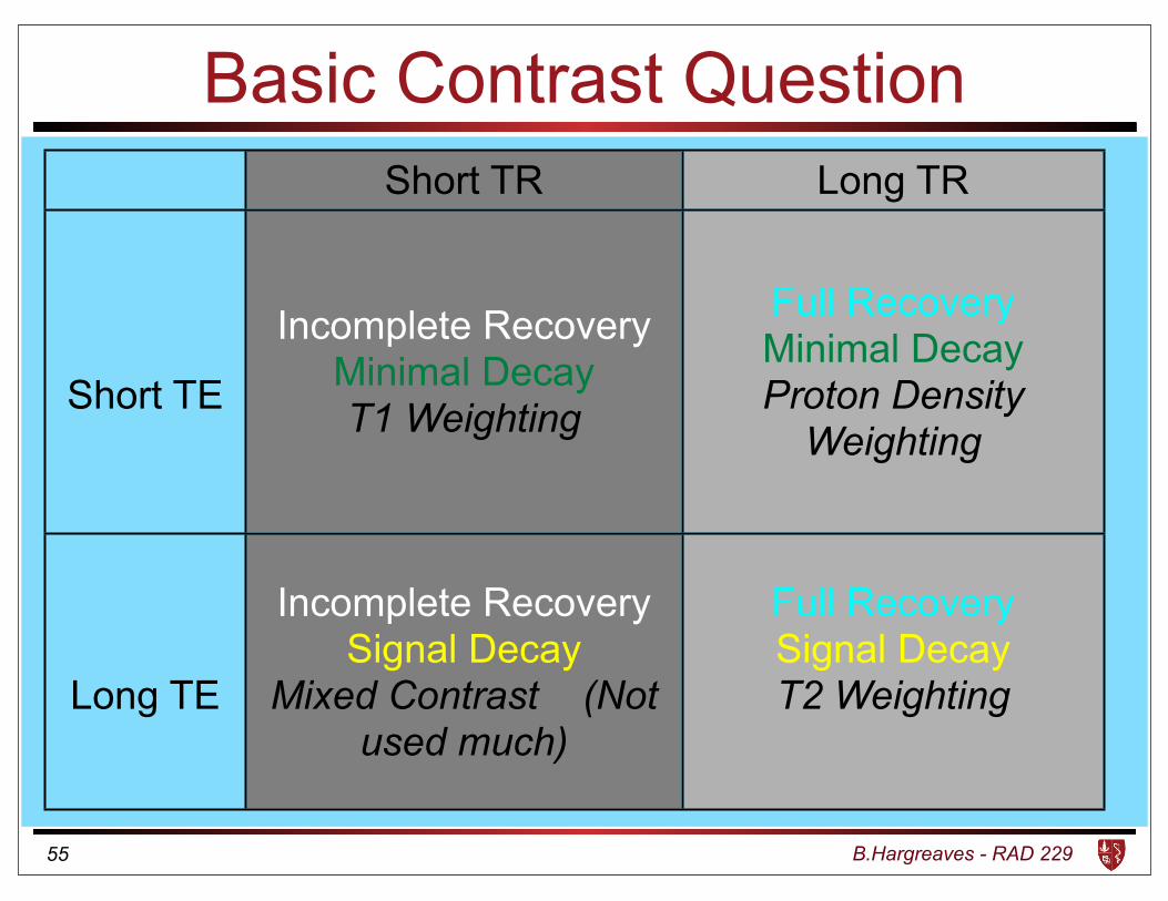
Basic Contrast QuestionShort TR Long TR

Short TE

Incomplete RecoveryMinimal DecayT1 Weighting

Full RecoveryMinimal DecayProton Density

Weighting

Long TE

Incomplete RecoverySignal Decay

Mixed Contrast (Not used much)

Full RecoverySignal DecayT2 Weighting

55


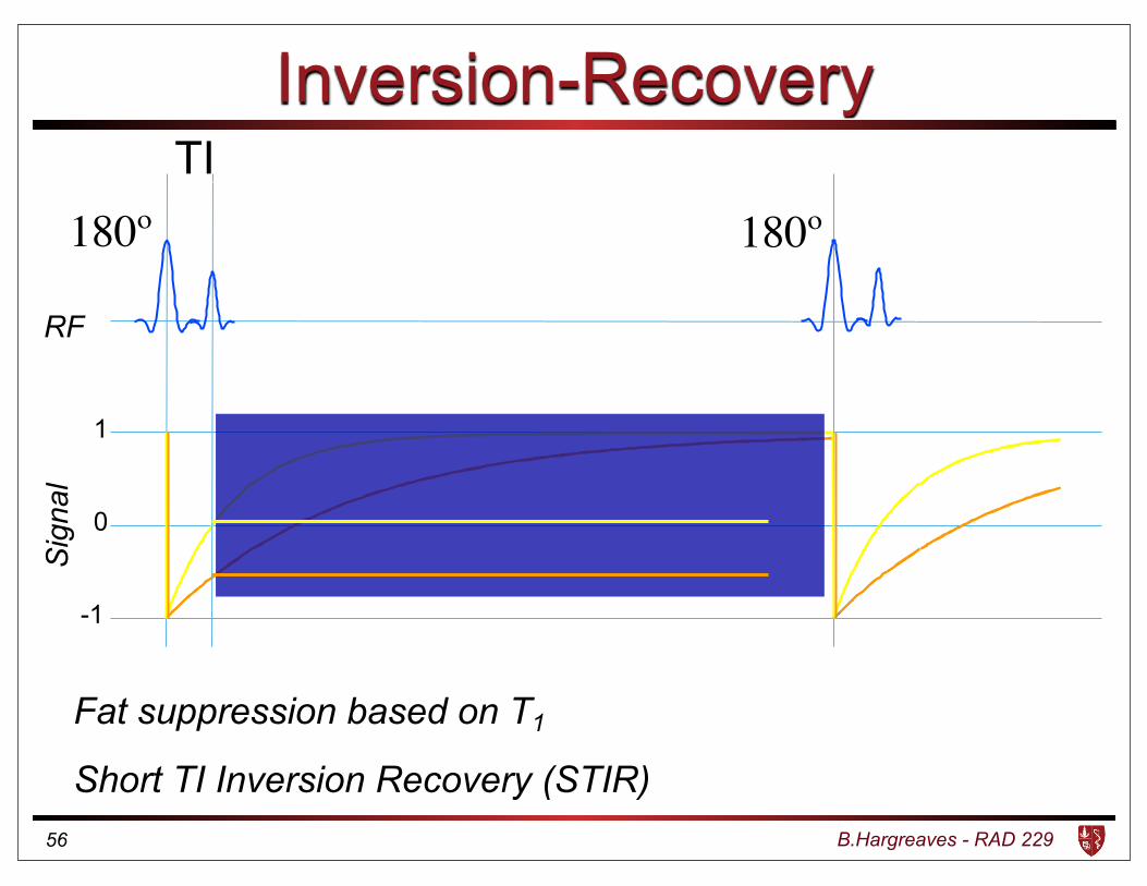
Inversion-Recovery

180º 180º

RF

Sig

nal

1

-1

0

• Fat suppression based on T1

• Short TI Inversion Recovery (STIR)

TI

56


Long Inversion Time (TI) - FLAIR

Long TI suppresses fluid signal57


Signal Question

• Inversion Recovery Sequence:

• TR = 1s, TI = 0.5s, TE=50ms

• What is the signal for T1=0.5s, T2=100ms?

58

180º 180º

RF

TI

TE

TR


Steady-State Sequences• Repeated sequences always lead to a “steady state”

• Sometimes includes equilibrium (easier)

• Otherwise trace magnetization and solve equations

• Example: Small-tip, TE=0

59

Mz(TR) = M0 + [Mz(TE)�M0]e�TR/T1

Mz(TE) = Mz(TR) cos↵

Mz(TR) = M01� e�TR/T1

1� cos↵Combining...

...“TR” “TE”


SNR: Signal-to-Noise Ratio

• Signal: Desired voltage in coil

• Noise: Thermal, electronic

• Thermal dominates, depends on coil, patient size

• SNR = average signal / σ

• Gaussian noise (FT is gaussian)

• N averages = sqrt(N) increase• Magnitude noise is Rician; can obtain σ

60

Signal

Noise


Low SNR High SNR

SNRSNR is the major limitation for MRI

61


Averaging

• Noise is uncorrelated

• When adding two signals:

• Signal portion M adds, to 2M

• Noise variance σ2 adds, increases to 2σ2

• Noise σ increases by square-root of 2

• SNR changes from M/σ to 1.4 M/σ

• SNR increases with square-root of #averages

62


Forms of Averaging

• NEX - simple averaging

• Decreased bandwidth/pixel (longer A/D time)

• Increased FOV

• Phase-encode direction

• Slice direction (3D)

• Readout direction (same BW!)

• Increased matrix - but changes resolution!

63


Imaging Factors Influencing SNR

• Voxel size (spatial resolution)

• Acquisition time (NEX, BW)

• Polarization or Field strength

• RF coil

• Subject size

• Pulse sequence and parameters

• Receive Electronics (Ideally insignificant)

64


Voxel Size Example

Full High Resolution 2x Increase (all 3 axes) 4x Increase (slice)

65


SNR and Field Strength

Sagittal T2 RARE: SNR Ratio = 1.7

1.5T 3.0T

66


Sensitive Volume

Target Region

Coil

Coil Sensitivity

• Signal decreases further from coil

• Noise volume increases with coil size

• Smaller coils also limit FOV and aliasing

• Larger coils not ideal

67


SNR vs Resolution vs Scan TimeHigh SNR

High Resolution(Small Voxels)

Short Scan Time

€

SNR ∝ Voxel Volume ⋅ Tacq

68


SNR Efficiency

• Often want to compare SNR of different sequences

• If times differ, comparison can be made fair by use of SNR efficiency:

• In many cases:

69

⌘SNR =SNRpTscan

⌘SNR =SNRpTR


SNR Question

• Compare the SNR efficiency of two pulse sequences, assuming the signal level is constant:• Spin Echo, 8echoes, 32.25 kHz bandwidth, TR=100ms

• Simple gradient echo, 62.5 kHz bandwidth, TR=5ms

• Signal level would NOT be constant, so this is harder!

70

⌘SNR / 1p62.5 · 5

= 0.057

⌘SNR /r

8

32.25 · 100 = 0.050


Pulse Sequences

• Gradient Echo Sequences

• Spin Echo Sequences

• (We will expand on these a lot!)

71


Gradient Echo Pulse Sequence

RF

Gz

Gy

Gx

Signal

TE

Gradient Echo

Flip Angle

72


Spin Echo Pulse Sequence

RF

Gz

Gy

Gx

Signal

180º TE ~ 8+ ms

73


Summary ~ EE369B

• Overview of NMR

• Hardware

• Image formation and k-space


• Signals and contrast

• Signal-to-Noise Ratio (SNR)

• Pulse Sequences

74

Documents

RAD 229: MRI Signals - Stanford Universityweb.stanford.edu/class/rad229/Notes/0-BasicMR-Review.pdf · B.Hargreaves - RAD 229 Lectures • 75 min lectures -- Notes online at website