Embed Size (px)
Citation preview

R. Sparvoli – MAPS 2009 -
Perugia
Outline of the lecture
Lecture 2:Lecture 2:
• Sources of background and their rejection
• Efficiencies & Contaminations• Absolute fluxes• Conclusions

R. Sparvoli – MAPS 2009 -
Perugia
Lecture 2:Lecture 2:Sources of background and
their rejection
Antiprotons
R. Sparvoli – MAPS 2009 -
Perugia
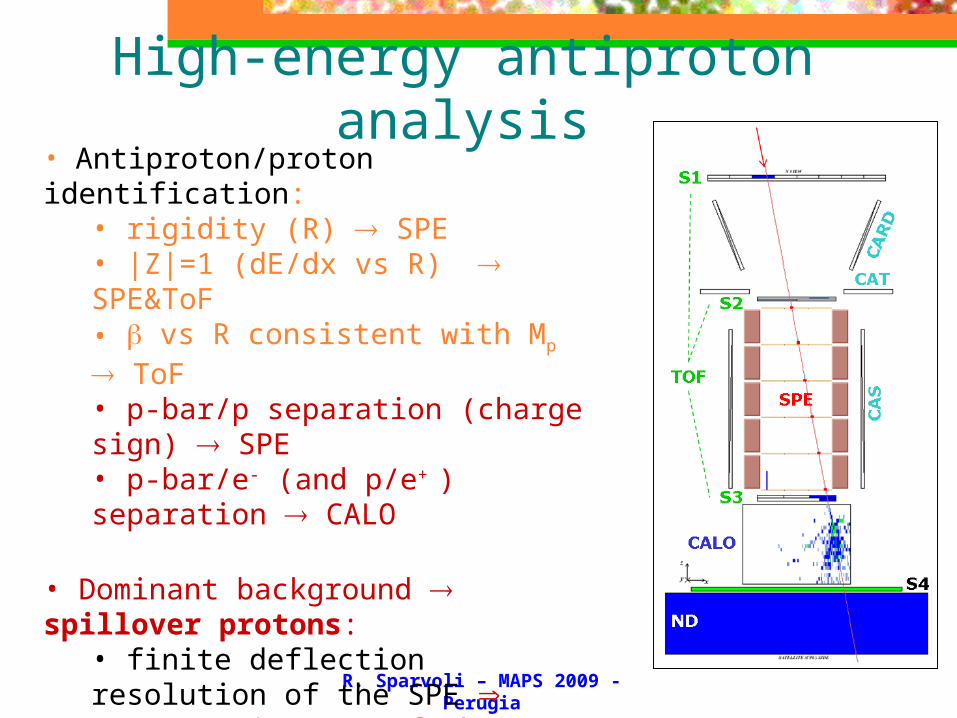
High-energy antiproton analysis
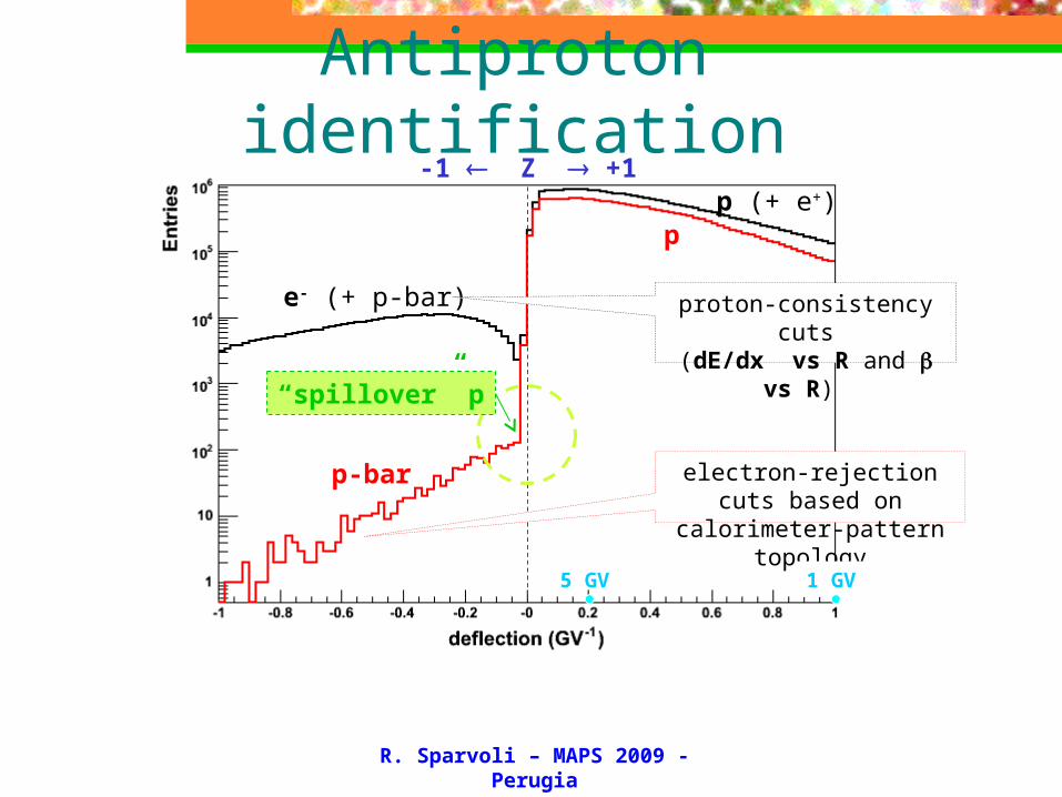
• Antiproton/proton identification:• rigidity (R) SPE• |Z|=1 (dE/dx vs R) SPE&ToF• vs R consistent with Mp ToF• p-bar/p separation (charge sign) SPE• p-bar/e- (and p/e+ ) separation CALO
• Dominant background spillover protons:
• finite deflection resolution of the SPE wrong assignment of charge-sign @ high energy • proton spectrum harder than antiproton p/p-bar increase for increasing energy (103 @1GV, 104 @100GV)
Required strong TRK selection
R. Sparvoli – MAPS 2009 -
Perugia
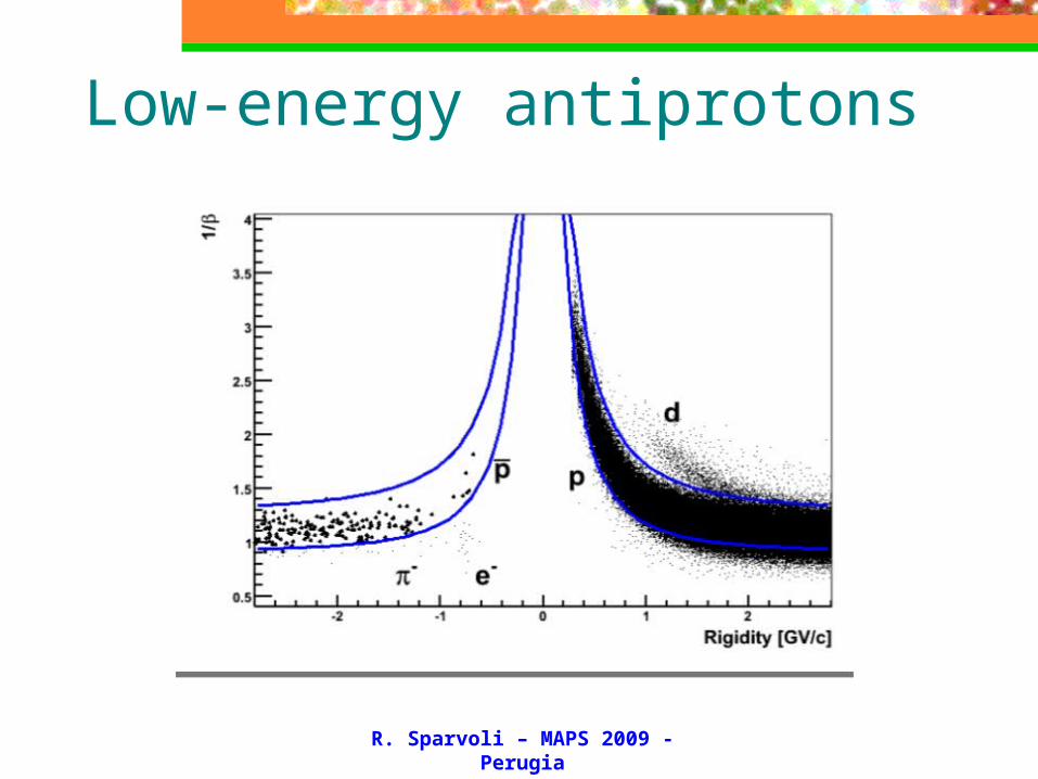
Low-energy antiprotons
R. Sparvoli – MAPS 2009 -
Perugia
GV-1
GV-1
GV-1
ee--
ee--
ee++
ee++
pp
pp
pp
pp
pp
pp
αα
R. Sparvoli – MAPS 2009 -
Perugia
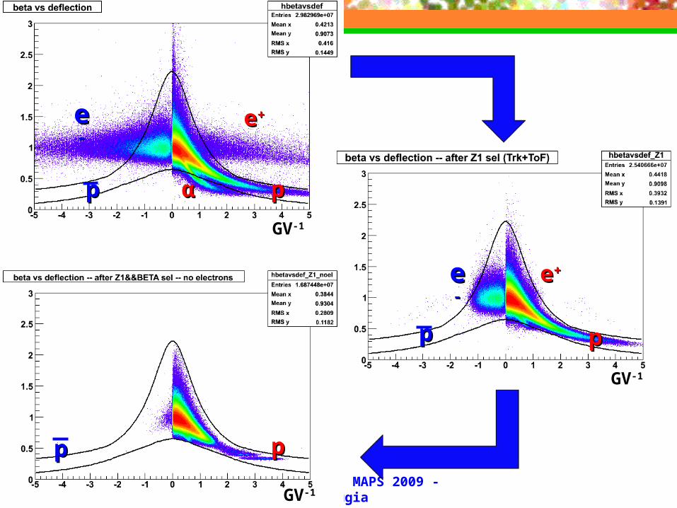
Antiproton identification
e- (+ p-bar)
p-bar
p
-1 Z +1
“spillover” p
p (+ e+)
proton-consistency cuts(dE/dx vs R and vs R)
electron-rejection cuts based on calorimeter-pattern topology
1 GV5 GV
R. Sparvoli – MAPS 2009 -
Perugia
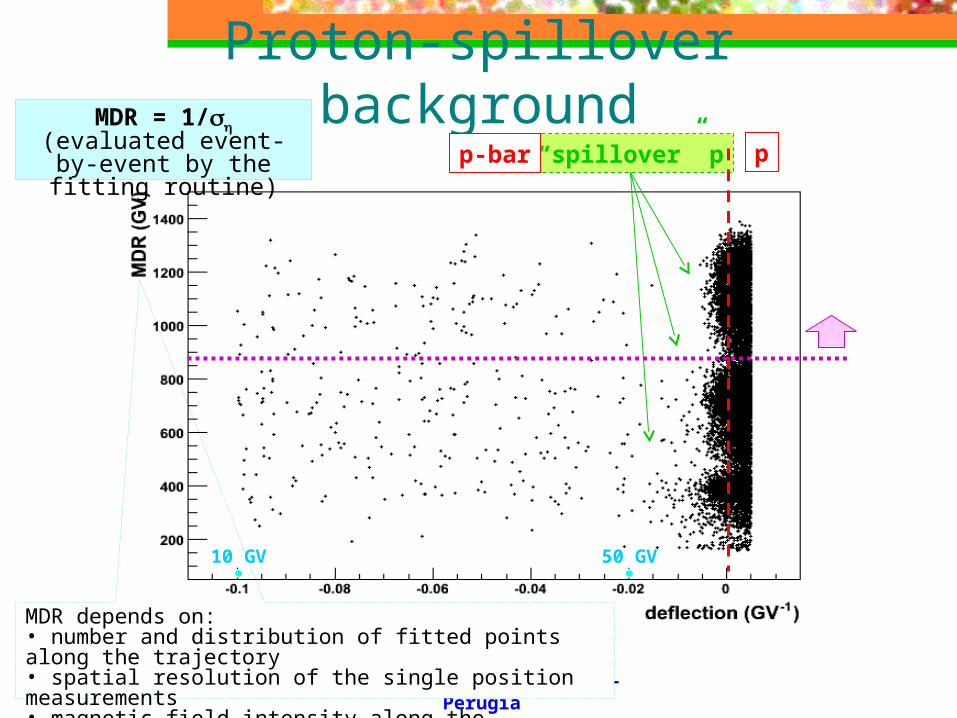
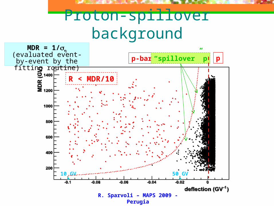
Proton-spillover background
MDR depends on:• number and distribution of fitted points along the trajectory• spatial resolution of the single position measurements• magnetic field intensity along the trajectory
“spillover” pp-bar p
10 GV 50 GV
MDR = 1/(evaluated event-by-event by the fitting
routine)
R. Sparvoli – MAPS 2009 -
Perugia
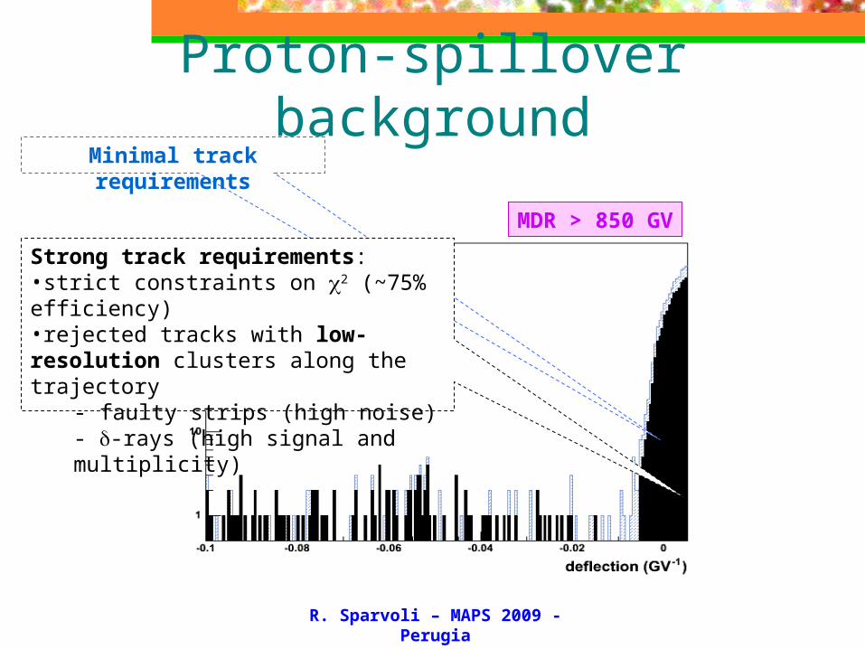
MDR > 850 GV
Minimal track requirements
Strong track requirements:•strict constraints on 2 (~75% efficiency)•rejected tracks with low-resolution clusters along the trajectory
- faulty strips (high noise)- -rays (high signal and multiplicity)
Proton-spillover background
R. Sparvoli – MAPS 2009 -
Perugia
Proton-spillover background
p-bar p“spillover” p
10 GV 50 GV
MDR = 1/(evaluated event-by-event by the fitting
routine)
R < MDR/10
R. Sparvoli – MAPS 2009 -
Perugia
Spillover as a limit to the maximum energy limit
The antiproton measurements are limited by the existence of the spillover effect;There is need of very stringeng tracking cuts (chi-square of the track, MDR, quality..) to separate spillover protons from antiprotons;
the maximum energy achieved by an instrument is defined as the energy where the signal is well separated from the spillover;For PAMELA, this limit is set to ~ 200 GeV.

R. Sparvoli – MAPS 2009 -
Perugia
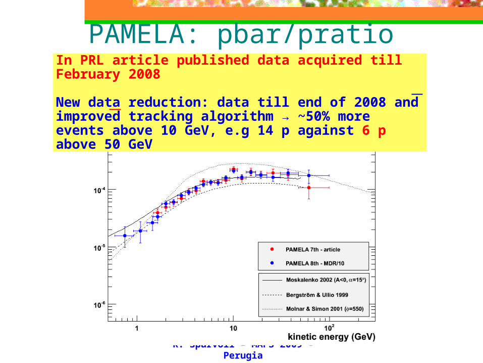
PAMELA: pbar/pratioPRL 102, 051101 (2009)
R. Sparvoli – MAPS 2009 -
Perugia
PAMELA: pbar/pratioIn PRL article published data acquired till February 2008
New data reduction: data till end of 2008 and improved tracking algorithm → ~50% more events above 10 GeV, e.g 14 p against 6 p above 50 GeV

Positrons
R. Sparvoli – MAPS 2009 -
Perugia
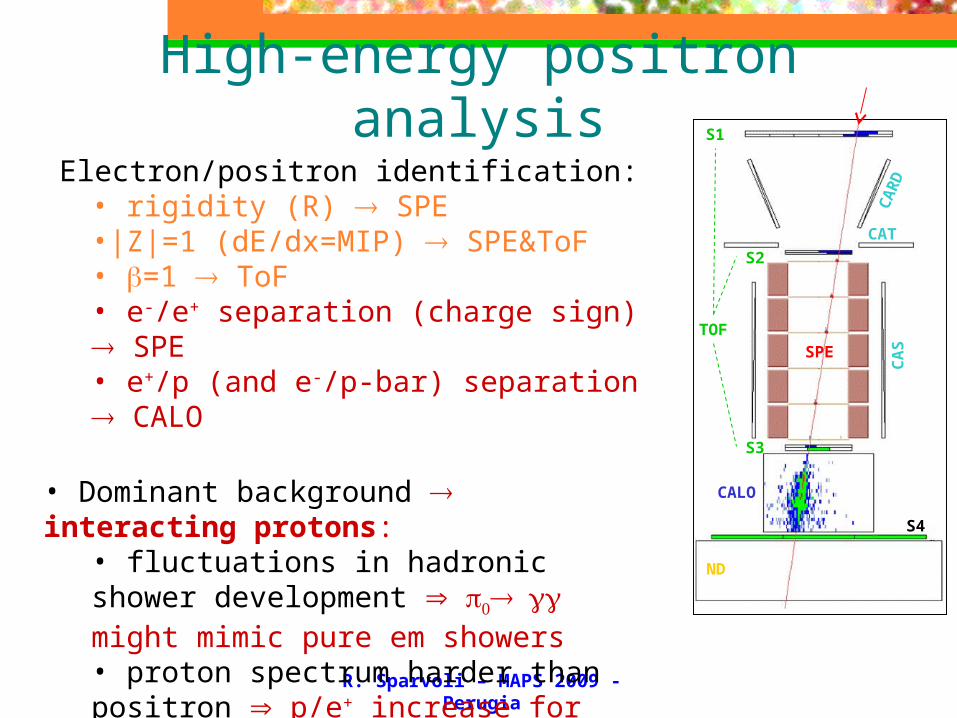
High-energy positron analysis Electron/positron identification:
• rigidity (R) SPE •|Z|=1 (dE/dx=MIP) SPE&ToF• =1 ToF• e-/e+ separation (charge sign) SPE• e+/p (and e-/p-bar) separation CALO
• Dominant background interacting protons:
• fluctuations in hadronic shower development might mimic pure em showers• proton spectrum harder than positron p/e+ increase for increasing energy (103 @1GV 104 @100GV)
Required strong CALO selection
S1
S2
CALO
S4
CA
RD
CA
S
CAT
TOFSPE
S3
ND
R. Sparvoli – MAPS 2009 -
Perugia
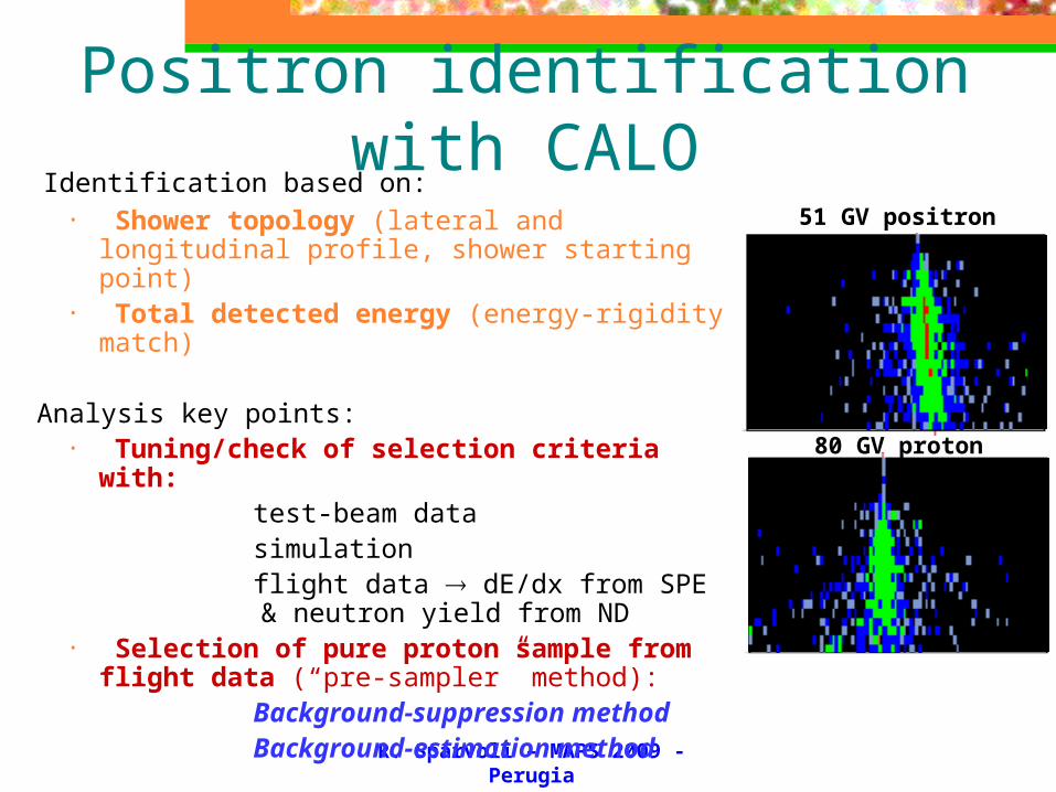
Positron identification with CALO
Identification based on:• Shower topology (lateral and longitudinal
profile, shower starting point)• Total detected energy (energy-rigidity
match)
Analysis key points:• Tuning/check of selection criteria with:
test-beam data simulation flight data dE/dx from SPE &
neutron yield from ND• Selection of pure proton sample from
flight data (“pre-sampler” method): Background-suppression
method Background-estimation
method
51 GV positron
80 GV proton
R. Sparvoli – MAPS 2009 -
Perugia
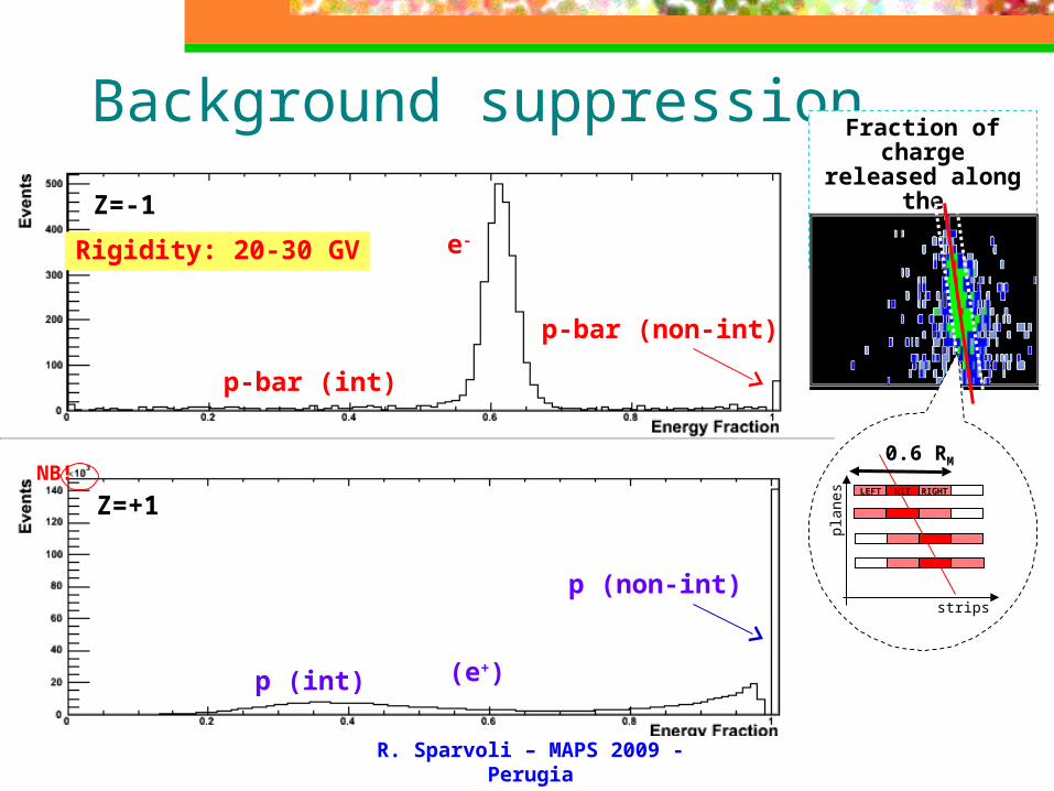
Background suppressionFraction of charge released along the calorimeter track
(e+)
p (non-int)
p (int)
NB!
p-bar (int)
e-
p-bar (non-int)
Z=-1
Z=+1
Rigidity: 20-30 GV
LEFT HIT RIGHT
strips
plan
es
0.6 RM

R. Sparvoli – MAPS 2009 -
Perugia
Fraction of charge released along the calorimeter track
(e+)
p (non-int)
p (int)
NB!
p-bar (int)
e-
p-bar (non-int)
Z=-1
Z=+1
Rigidity: 20-30 GV
+Constraints on:
Energy-momentum match
e+
p
p-bar
e-
Z=-1
Z=+1
Rigidity: 20-30 GV

R. Sparvoli – MAPS 2009 -
Perugia
e+
p
p-bar
e-
Z=-1
Z=+1
Rigidity: 20-30 GV
Fraction of charge released along the calorimeter track
+Constraints on:
Energy-momentum match
Shower starting-point
Longitudinal profile
e+
p
e-Rigidity: 20-30 GV
Z=-1
Z=+1
Lateral profile
BK-suppression
method
R. Sparvoli – MAPS 2009 -
Perugia
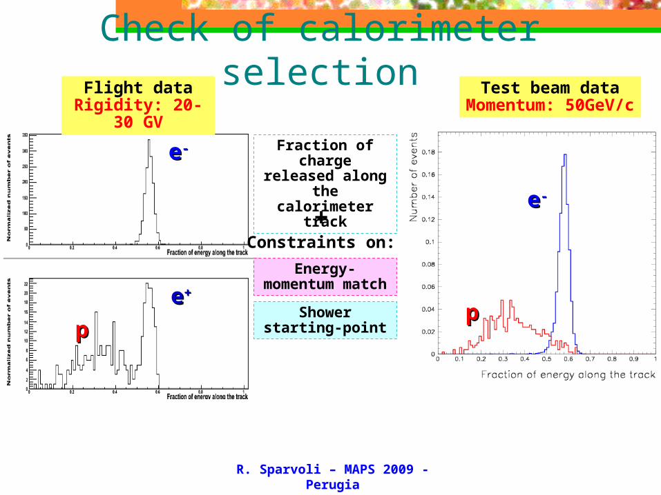
Check of calorimeter selection
pppp
Flight dataRigidity: 20-30
GV
Test beam dataMomentum: 50GeV/c
ee--
Fraction of charge released along the calorimeter track
+Constraints on:
Energy-momentum match
Shower starting-point
ee--
ee++
R. Sparvoli – MAPS 2009 -
Perugia
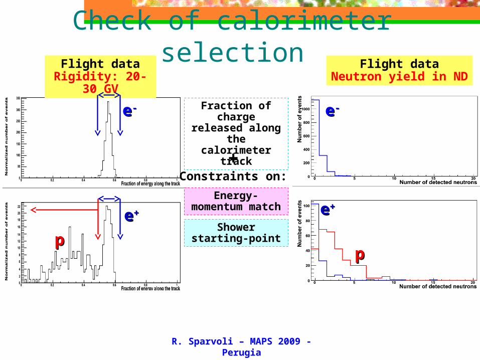
Check of calorimeter selection
pp
Flight dataRigidity: 20-30
GV
ee--
ee++
Fraction of charge released along the calorimeter track
+Constraints on:
Energy-momentum match
Shower starting-point
ee--
ee++
pp
Flight dataNeutron yield in ND
R. Sparvoli – MAPS 2009 -
Perugia
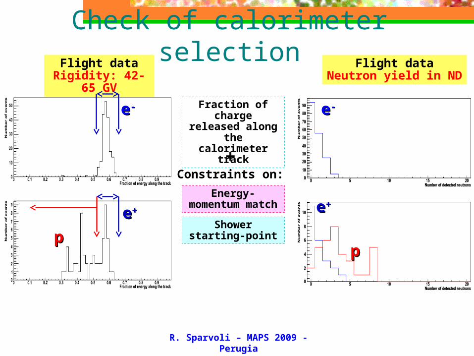
Check of calorimeter selection
pp
Flight dataRigidity: 42-65
GV
ee--
ee++
Fraction of charge released along the calorimeter track
+Constraints on:
Energy-momentum match
Shower starting-point
ee--
ee++
pp
Flight dataNeutron yield in ND
R. Sparvoli – MAPS 2009 -
Perugia
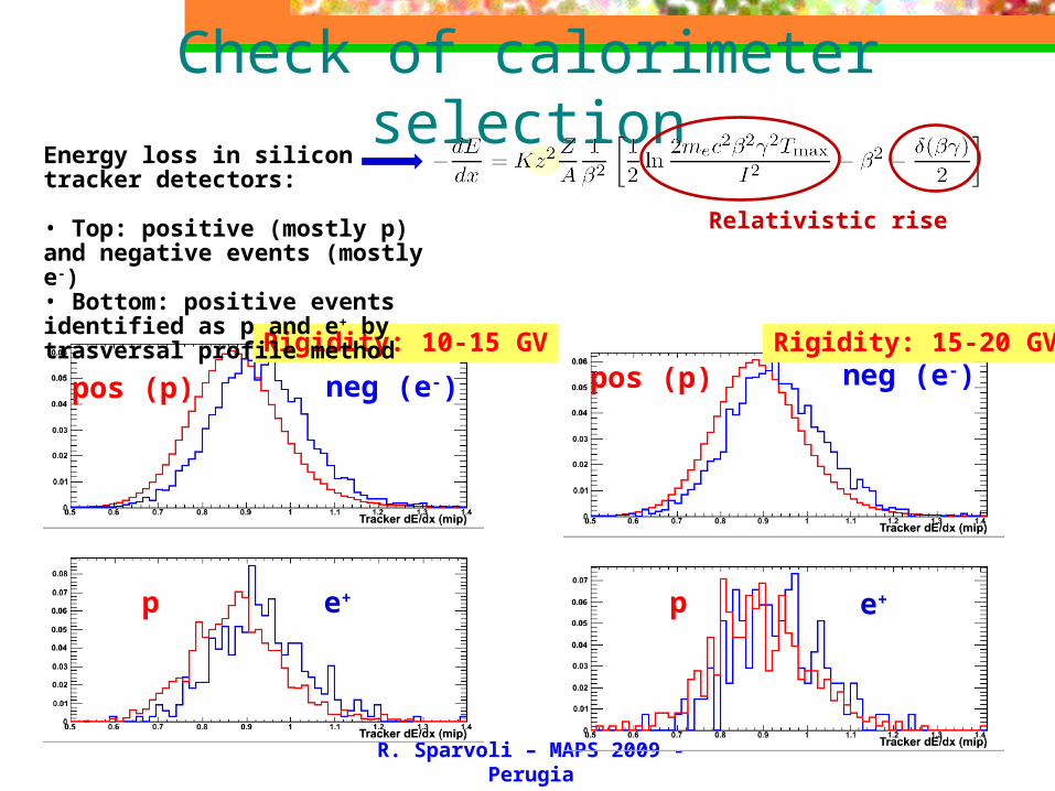
Check of calorimeter selection
Rigidity: 10-15 GV Rigidity: 15-20 GV
neg (e-)
e+e+p
pos (p)
p
neg (e-)pos (p)
Energy loss in silicon tracker detectors:
• Top: positive (mostly p) and negative events (mostly e-)• Bottom: positive events identified as p and e+ by trasversal profile method
Relativistic rise
R. Sparvoli – MAPS 2009 -
Perugia
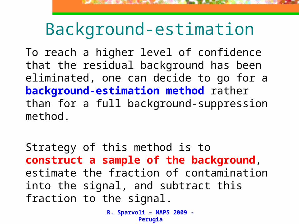
Background-estimationTo reach a higher level of confidence that the residual background has been eliminated, one can decide to go for a background-estimation method rather than for a full background-suppression method.
Strategy of this method is to construct a sample of the background, estimate the fraction of contamination into the signal, and subtract this fraction to the signal.
R. Sparvoli – MAPS 2009 -
Perugia
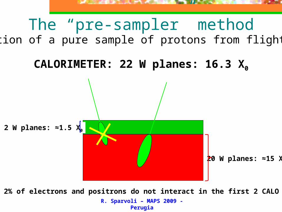
2 W planes: ≈1.5 X0
20 W planes: ≈15 X0
CALORIMETER: 22 W planes: 16.3 X0
The “pre-sampler” methodSelection of a pure sample of protons from flight data
Only 2% of electrons and positrons do not interact in the first 2 CALO planes
R. Sparvoli – MAPS 2009 -
Perugia
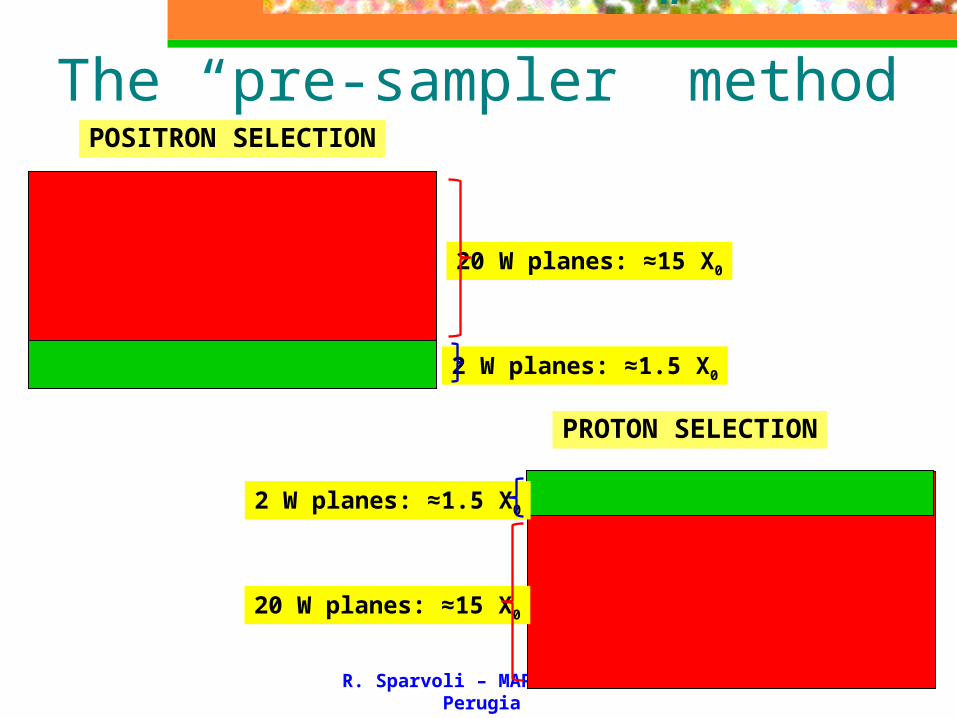
The “pre-sampler” methodPOSITRON SELECTION
PROTON SELECTION
2 W planes: ≈1.5 X0
20 W planes: ≈15 X0
20 W planes: ≈15 X0
2 W planes: ≈1.5 X0
R. Sparvoli – MAPS 2009 -
Perugia
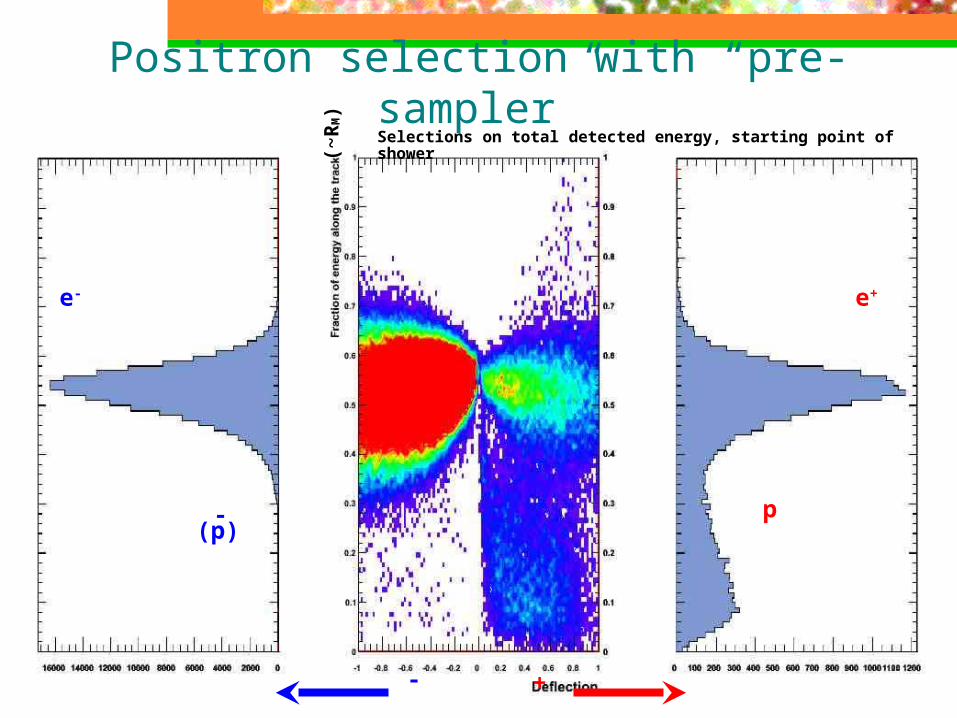
(~R
M)
+-
Selections on total detected energy, starting point of shower
e- e+
(p)- p
Positron selection with “pre-sampler”
R. Sparvoli – MAPS 2009 -
Perugia
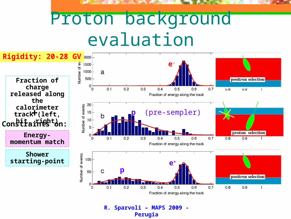
Proton background evaluation
Rigidity: 20-28 GV
Fraction of charge released along the
calorimeter track (left, hit, right)
+Constraints on:
Energy-momentum match
Shower starting-pointe+
p (pre-sempler)
e-
p
R. Sparvoli – MAPS 2009 -
Perugia
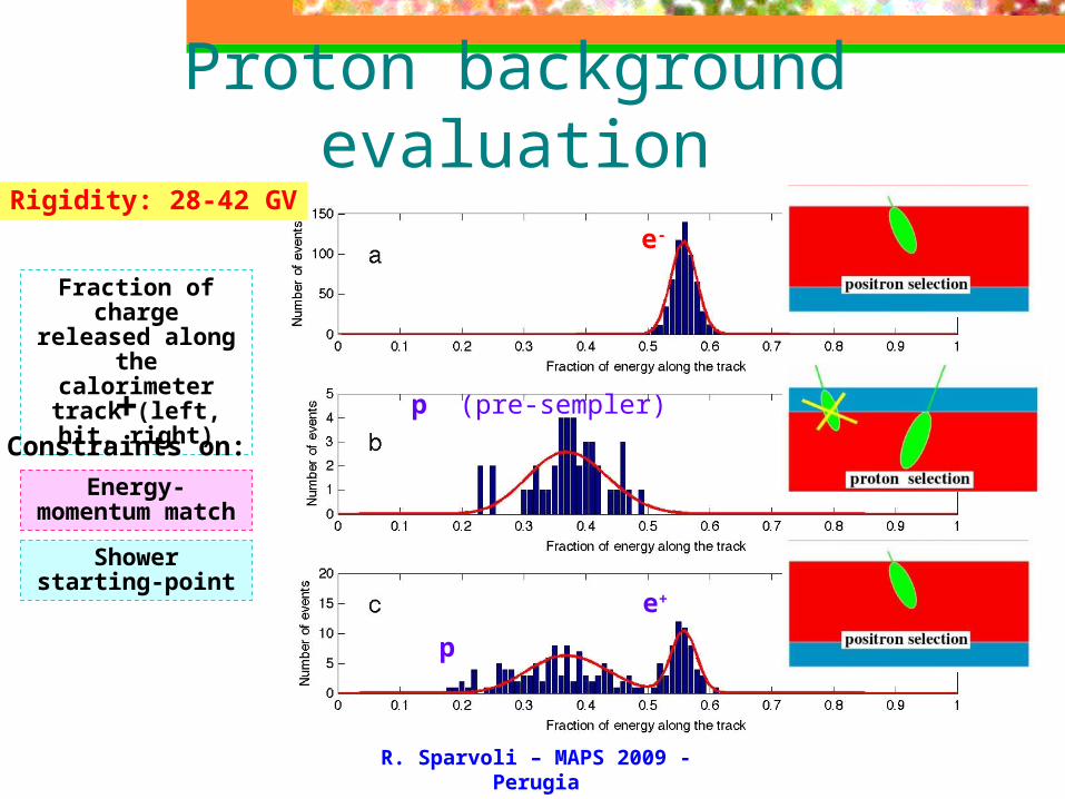
Proton background evaluation
Rigidity: 28-42 GV
Fraction of charge released along the
calorimeter track (left, hit, right)
+Constraints on:
Energy-momentum match
Shower starting-point
e+
p (pre-sempler)
e-
p
R. Sparvoli – MAPS 2009 -
Perugia
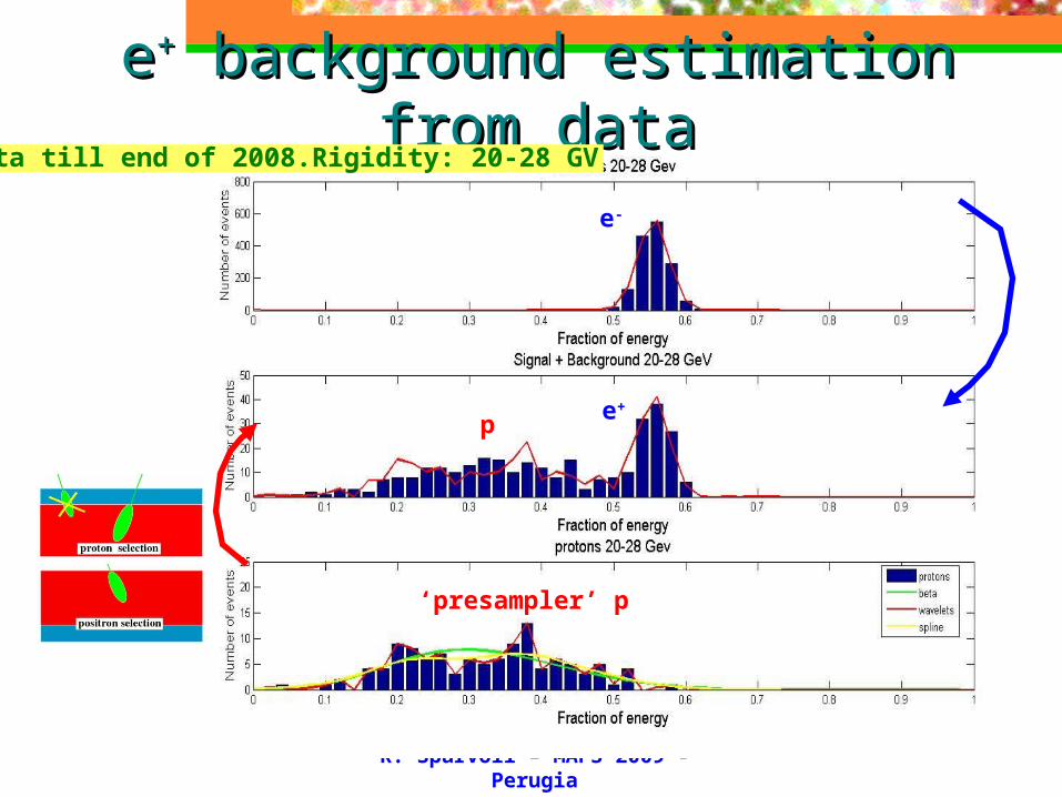
ee++ background estimation from background estimation from datadata
e-
‘presampler’ p
e+
p
Data till end of 2008.Rigidity: 20-28 GV
R. Sparvoli – MAPS 2009 -
Perugia
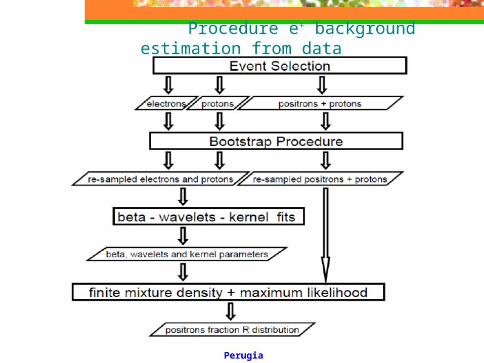
Procedure e+ background estimation from data
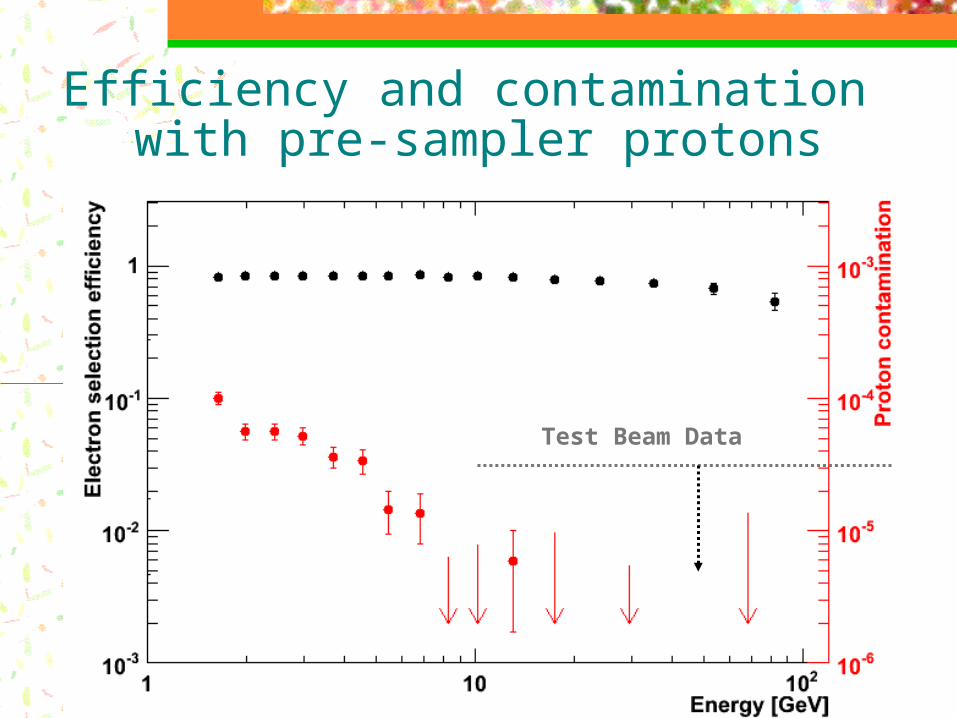
Efficiency and contamination with pre-sampler protons
Test Beam Data
R. Sparvoli – MAPS 2009 -
Perugia
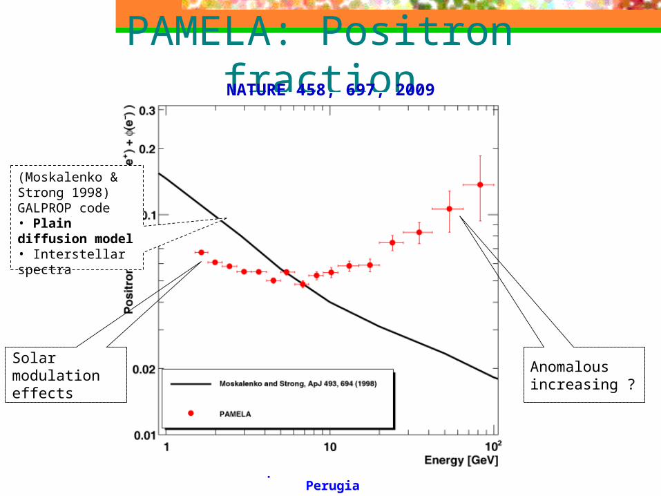
PAMELA: Positron fraction
Solar modulation effects
Anomalous increasing ?
(Moskalenko & Strong 1998) GALPROP code • Plain diffusion model • Interstellar spectra
NATURE 458, 697, 2009

R. Sparvoli – MAPS 2009 -
Perugia
PAMELA: Positron fractionNATURE 458, 697, 2009
R. Sparvoli – MAPS 2009 -
Perugia
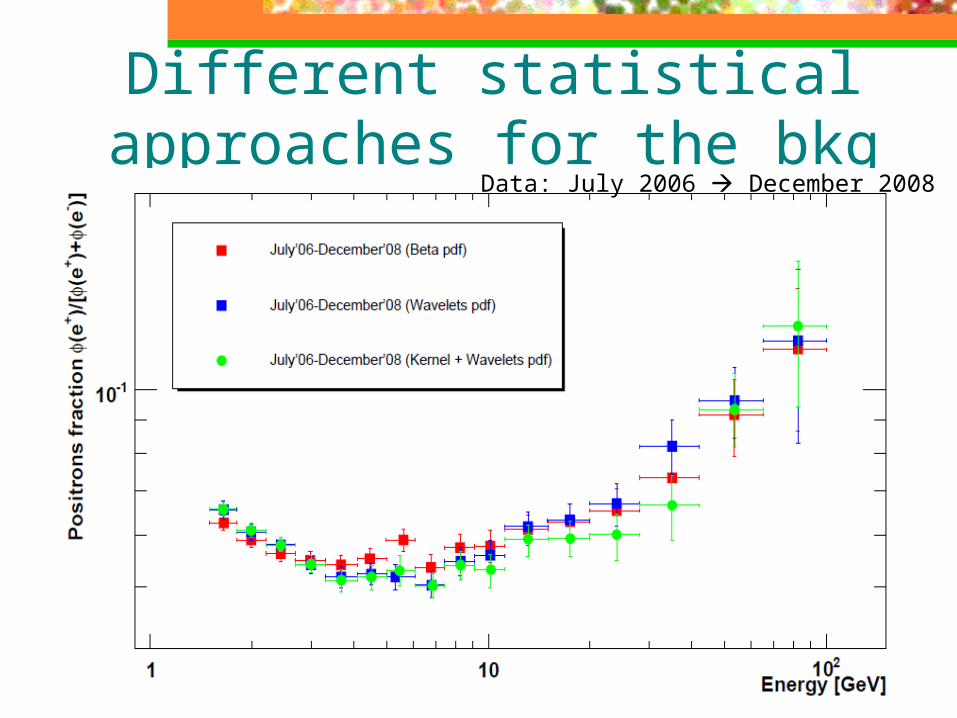
Different statistical approaches for the bkg
Data: July 2006 December 2008
R. Sparvoli – MAPS 2009 -
Perugia
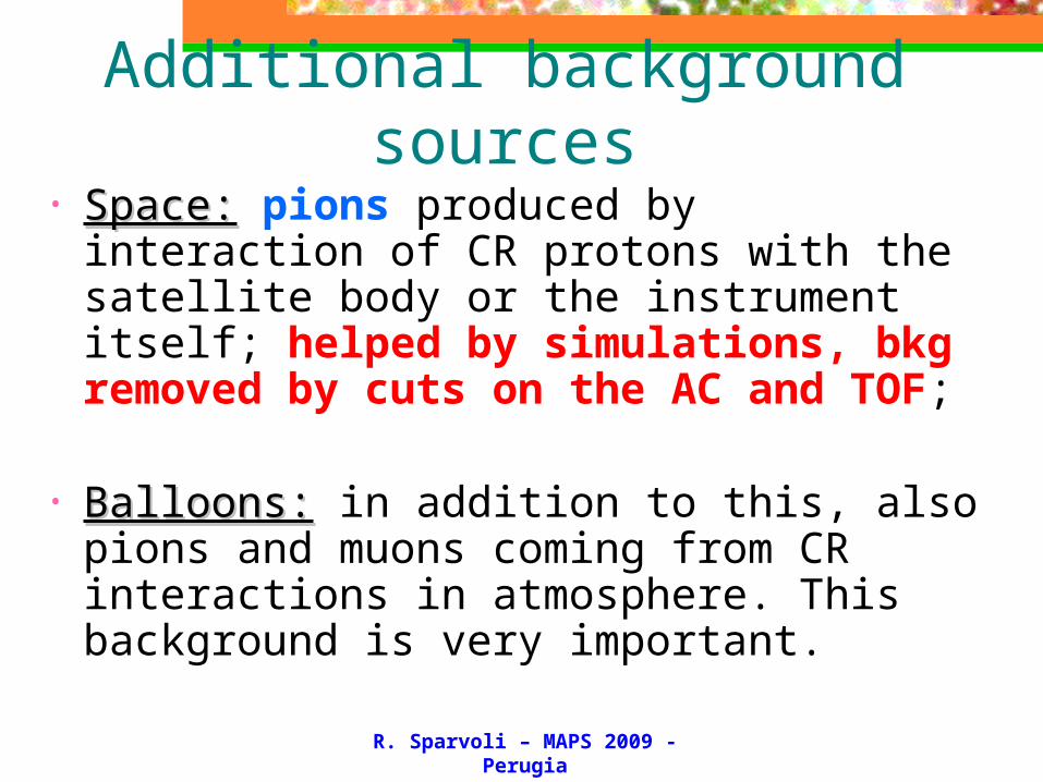
Additional background sources
• Space:Space: pions produced by interaction of CR protons with the satellite body or the instrument itself; helped by simulations, bkg removed by cuts on the AC and TOF;
• Balloons:Balloons: in addition to this, also pions and muons coming from CR interactions in atmosphere. This background is very important.

R. Sparvoli – MAPS 2009 -
Perugia
Lecture 2:Lecture 2:
Efficiencies & Contaminations

R. Sparvoli – MAPS 2009 -
Perugia
Efficiency of selection cuts
We have seen how different information from detectors bring to particle identification. All selection criteria have to be combined together to select a specific particle type.
To be able to compute particle ratios and fluxes, we must know the efficiency of every selection cut, namely the probability that a good event passes that selection cut.
The efficiencies will be combined together, and much attention must be put into correlations between selection cuts.
R. Sparvoli – MAPS 2009 -
Perugia
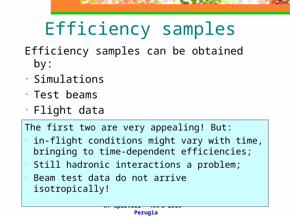
Efficiency samplesEfficiency samples can be obtained by:• Simulations• Test beams• Flight data
The first two are very appealing! But:- in-flight conditions might vary with time,
bringing to time-dependent efficiencies;- Still hadronic interactions a problem;- Beam test data do not arrive
isotropically!
R. Sparvoli – MAPS 2009 -
Perugia
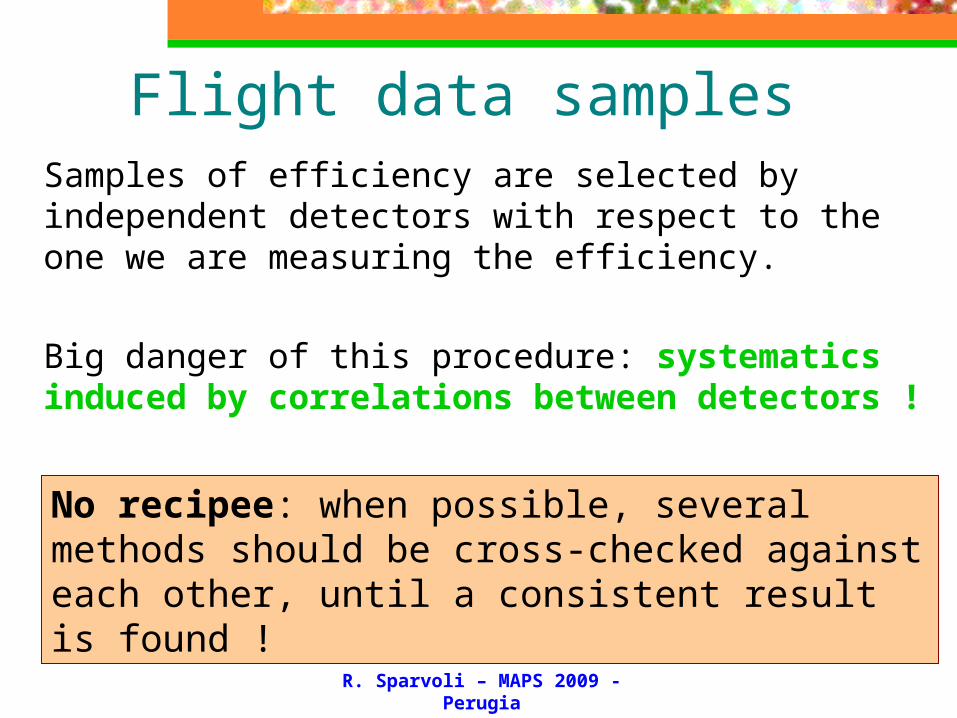
Flight data samplesSamples of efficiency are selected by independent detectors with respect to the one we are measuring the efficiency.
Big danger of this procedure: systematics induced by correlations between detectors !
No recipee: when possible, several methods should be cross-checked against each other, until a consistent result is found !
R. Sparvoli – MAPS 2009 -
Perugia
Example: tracker efficiency
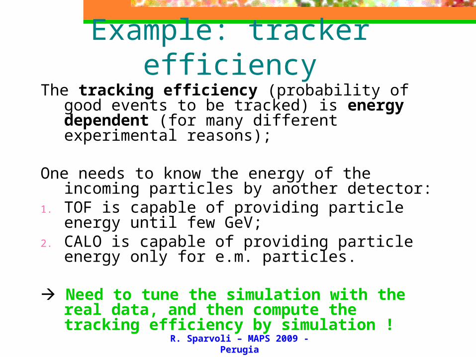
The tracking efficiency (probability of good events to be tracked) is energy dependent (for many different experimental reasons);
One needs to know the energy of the incoming particles by another detector:
1. TOF is capable of providing particle energy until few GeV;
2. CALO is capable of providing particle energy only for e.m. particles.
Need to tune the simulation with the real data, and then compute the tracking efficiency by simulation !
R. Sparvoli – MAPS 2009 -
Perugia
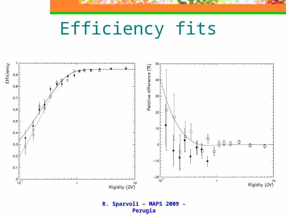
Efficiency fits
R. Sparvoli – MAPS 2009 -
Perugia
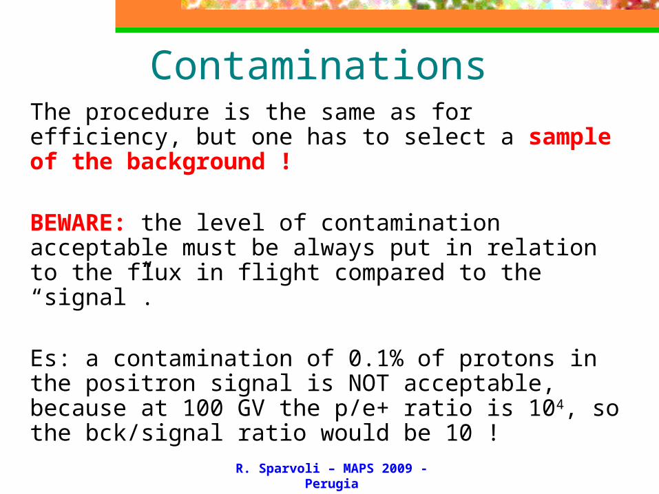
ContaminationsThe procedure is the same as for efficiency, but one has to select a sample of the background !
BEWARE: the level of contamination acceptable must be always put in relation to the flux in flight compared to the “signal”.
Es: a contamination of 0.1% of protons in the positron signal is NOT acceptable, because at 100 GV the p/e+ ratio is 104, so the bck/signal ratio would be 10 !

R. Sparvoli – MAPS 2009 -
Perugia
Lecture 2:Lecture 2:
Determination of fluxes
R. Sparvoli – MAPS 2009 -
Perugia
Final steps
Once the number of selected events has been obtained, and efficiencies of the selection cuts calculated, the final steps are:
1. derive the final number of events by correction for the selection efficiencies;2. include live time and geometrical factor in the calculation;3. propagate the flux at the top of the instrument, including energy loss in dead materials;4. eventually (balloon flights) propagate the flux at the top of atmosphere.

R. Sparvoli – MAPS 2009 -
Perugia
Correction for efficiencyThe selected events are distributed in energy bins,
fixed as a compromise between statistics and energy resolution of the instrument (pointless to have them much smaller than it!).
Since efficiencies are energy-dependent, the efficiency correction will be done bin per bin:
If does not vary significantly inside the bin, the correction will be easy and done at the center of gravity of the energy distribution of the events;
If varies significantly inside the bin, one has to obtain an “average efficiency value” inside the bin, by means of a weighting technique.
R. Sparvoli – MAPS 2009 -
Perugia
Particle fluxes
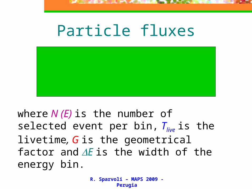
J (E) = 1 x N (E) Tlive x G x E
where N (E) is the number of selected event per bin, Tlive is the livetime, G is the geometrical factor and E is the width of the energy bin.
R. Sparvoli – MAPS 2009 -
Perugia
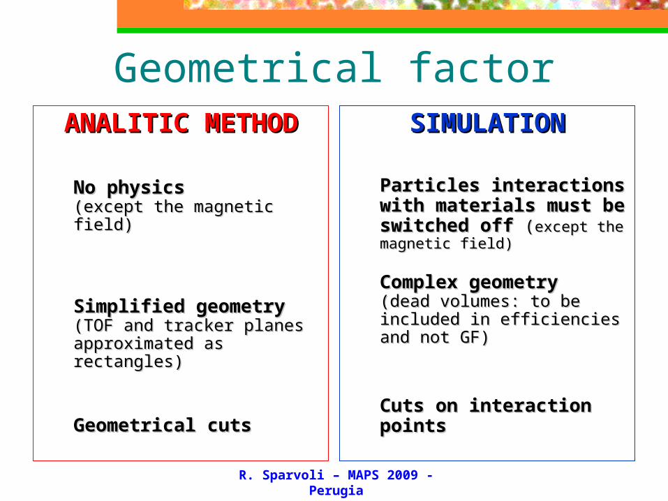
Geometrical factorANALITIC METHODANALITIC METHOD
No physicsNo physics (except the magnetic field)(except the magnetic field)
Simplified geometrySimplified geometry (TOF and tracker planes (TOF and tracker planes approximated as rectangles)approximated as rectangles)
Geometrical cutsGeometrical cuts
SIMULATIONSIMULATION
Particles interactions Particles interactions with materialswith materials must be must be switched offswitched off ((except the except the magnetic field)magnetic field)
Complex geometryComplex geometry (dead volumes: to be (dead volumes: to be included in efficiencies and included in efficiencies and not GF)not GF)
Cuts on interaction Cuts on interaction pointspoints
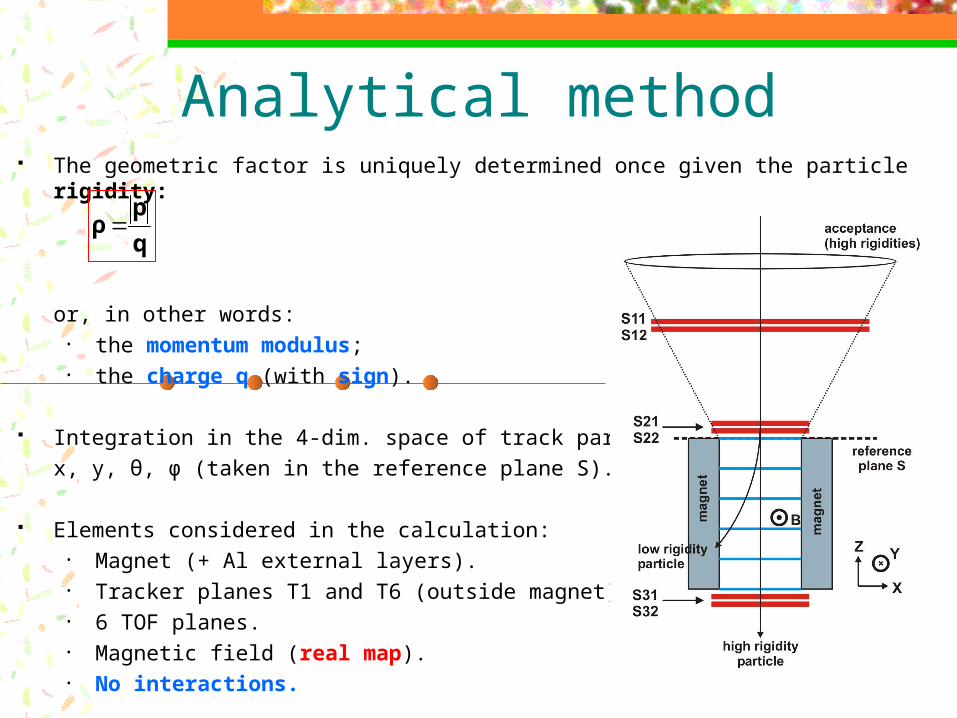
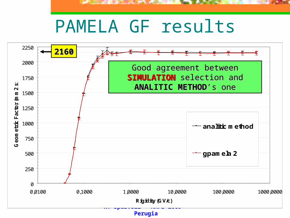
The geometric factor is uniquely determined once given the particle rigidity:
or, in other words:• the momentum modulus;• the charge q (with sign).
Integration in the 4-dim. space of track parametersx, y, θ, φ (taken in the reference plane S).
Elements considered in the calculation:• Magnet (+ Al external layers).• Tracker planes T1 and T6 (outside magnet).• 6 TOF planes.• Magnetic field (real map).• No interactions.
Analytical method
q
p ρ
R. Sparvoli – MAPS 2009 -
Perugia
0
250
500
750
1000
1250
1500
1750
2000
2250
0,0100 0,1000 1,0000 10,0000 100,0000 1000,0000
Rigidity (GV/c)
Geo
metr
ic F
acto
r (m
m2 s
r)(
analitic method
gpamela 2
PAMELA GF results
Good agreement between Good agreement between SIMULATIONSIMULATION selection and selection and ANALITIC METHODANALITIC METHOD’s one’s one
21602160

R. Sparvoli – MAPS 2009 -
Perugia
Spectra at top of the payload
Particles crossing the material above the tracking system lose energy by ionization and bremsstrahlung processes.
This changes the energy distribution of these particles; the spectra determined as in previous slide need to be extrapolated to the corresponding spectra at the top of the payload.In this extrapolation all the processes of energy loss have to be taken into account.
R. Sparvoli – MAPS 2009 -
Perugia
This is done with an iterative procedure: the spectra in the spectrometer are used as input spectra of a program which integrates, with a RungeKutta technique, the particle propagation equation for a depth t of radiation lengths equal to the material above the tracking system. The resulting spectra are compared with the ones found in the spectrometer and the differences are used to rescale the input spectra.
This iterative procedure goes on until the spectra propagated into the spectrometer coincide - in agreement within a few percent - with the experimental ones.
This technique is cross checked using the simulation of the payload.
Spectra at top of the payload
R. Sparvoli – MAPS 2009 -
Perugia
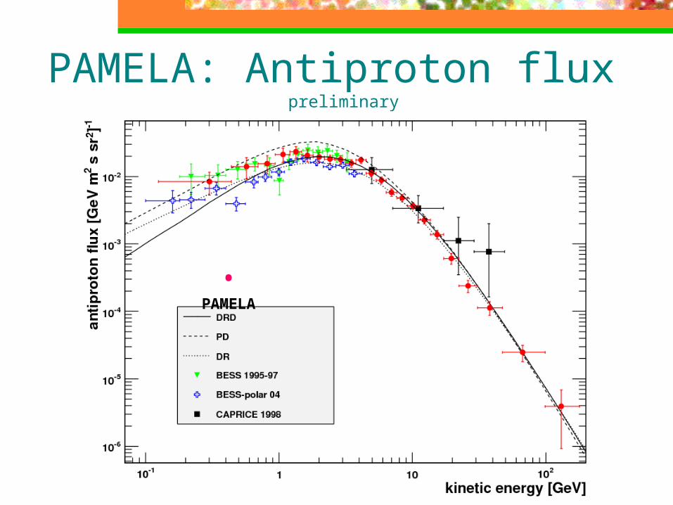
PAMELA: Antiproton flux preliminary
• PAMELA
R. Sparvoli – MAPS 2009 -
Perugia
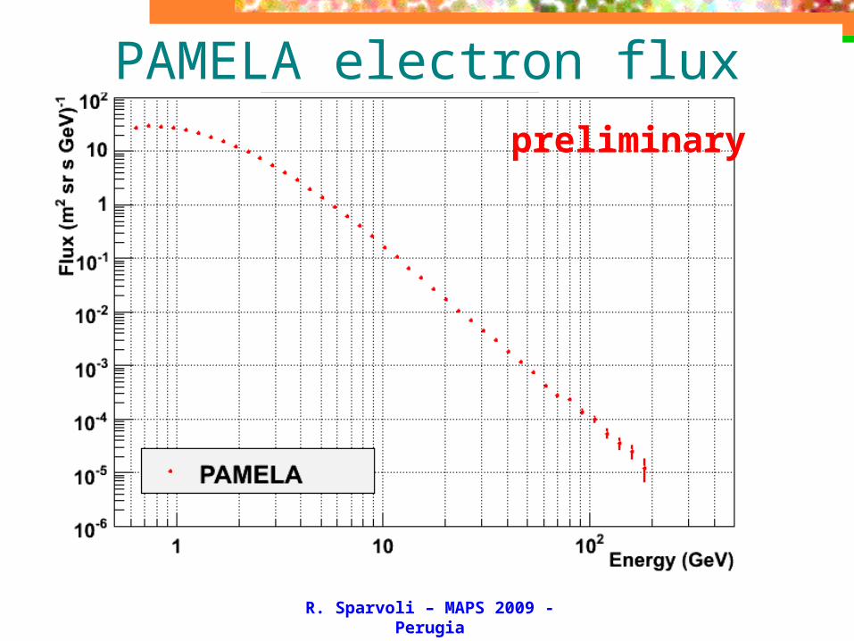
PAMELA electron fluxpreliminary
R. Sparvoli – MAPS 2009 -
Perugia
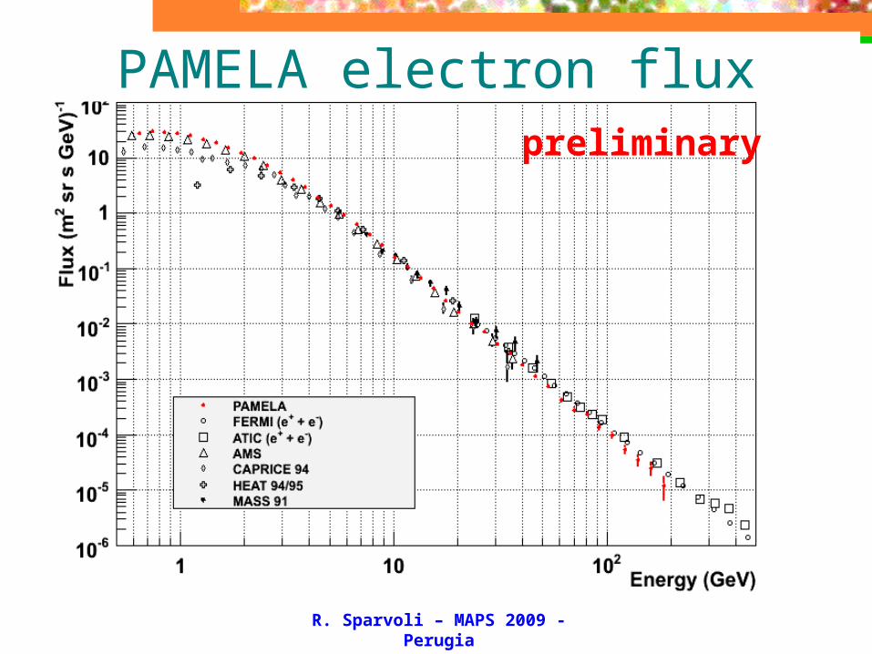
PAMELA electron fluxpreliminary
R. Sparvoli – MAPS 2009 -
Perugia
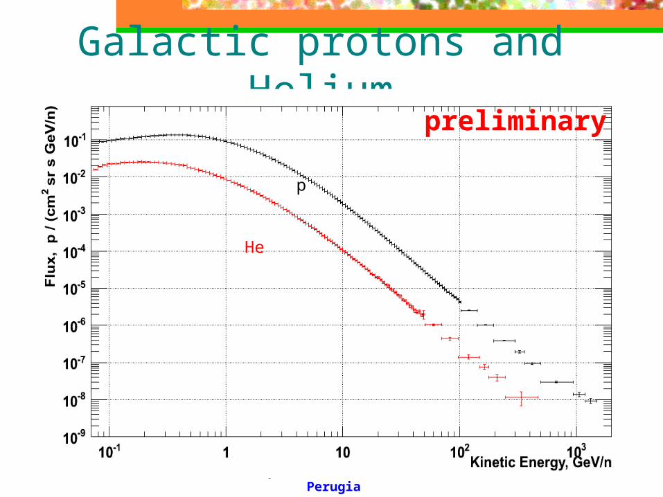
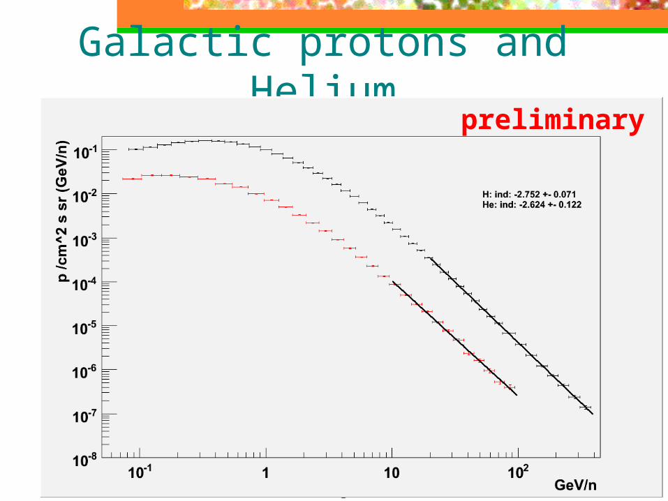
Galactic protons and Helium
p
He
preliminary
R. Sparvoli – MAPS 2009 -
Perugia
Galactic protons and Helium
preliminary
R. Sparvoli – MAPS 2009 -
Perugia
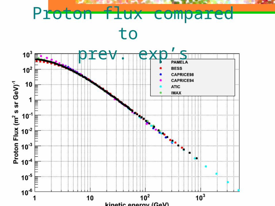
Proton flux compared to prev. exp’s
R. Sparvoli – MAPS 2009 -
Perugia
ConclusionsCosmic ray research in space is living a very exciting
time: many instruments in flight (PAMELA, AMS, AGILE, FERMI,..) are providing – and will provide – excellent data to answer important questions.
For the first time measurements of cosmic rays can be performed with the precision, statistics and temporal evolution needed to clarify many of the open problems in cosmology, astrophysics and solar terrestrial environment.
Especially the search for rare particles has – from a theoretical point of view – the potentiality for discovering new physics.
Task of the experimentalist is to provide high-quality data: the particle-physics technologies and methodologies used in space transformed the “once-pioneeristic” CR physics to a science of precision.

R. Sparvoli – MAPS 2009 -
Perugia
Courtesy of Neil Weiner