Embed Size (px)
Citation preview
ELECTRONIC TECHNOLOGY SERIES
R-F TRANSMISSION LINES
a
,, . ' ' .
4. ... • • 4J' • -:· ... , ·~·.' •
.... ,•.,'. ' , .. ,, . ,·;,
. -:~/ \:· .. ~: '' . ' ~.\: .
. ·.~ :/ ·. ·•: ., ., '
publication
l•

R-F TRANSMISSION
LINES
Edited by
Alexander Schure, Ph. D., Ed. D.
$1.25
JOHN F. RIDER PUBLISHER, INC. 480 Canal Street • New York 13, N.Y.
Copyright 1956 by
JOHN F. RIDER PUBLISHER, INC.
All rights reserved. This book or parts thereof may not be reproduced in any form or in any language
without permission of the publisher.
FIRST EDITION
Library of Congress Catalog Card No. 56-9744
Printed In the United States of America

PREFACE
An understanding of the fundamental concepts of transmission lines is essential to the electronic technician or engineer. Transmission lines are links in the chain of propagation or reception of r-f power. Regardless of the actual job that a particular kind of r-f transmission line accomplishes, some type of line will be used to carry radio frequency power in any complete communications system.
The book has been organized to help the student to understand the important ideas pertaining to the basic types of r-f transmission lines. A minimum of mathematical treatment has been employed, but the analyses are sufficiently extensive to permit the technician, practicing engineer, or advanced student to develop these fundamental concepts and basic applications to best advantage.
Specific attention has been given to the various types of line in common use; the problem of lumped and distributed constants; variations of constants; characteristic impedance; line termination; standing waves; standing wave ratio; input impedance; line losses; the half-wavelength line; the quarter-wavelength line; resonant lines; the Lecher wire line; supporting stubs; delay lines; and artificial transmission lines. The use of waveguides has been omitted from this text, because it is treated separately in another electronic technology book.
The content, then, is sufficient for an adequate understanding of both the theory and applications of this subject. A number of sample problems are given in sufficient detail, wherever applicable and pertinent, to permit the reader to apply the demonstrated procedures to situations that may confront them.
Grateful acknowledgement is made to the staff of New York Technical Institute for its assistance in the preparation of the manuscript for this book.
New York,N. Y. April 1956
V
A.S.

CONTENTS
Chapter Page
I Fundamental Concepts of Transmission Lines..................... I
2 Transmission Line Operation and Characteristics............ 9
3 Applications of Transmission Lines................................................ 39
vii

Chapter 1
FUNDAMENTAL CONCEPTS OF TRANSMISSION LINES
1. Introduction to Transmission Lines
A transmission line is exactly what its name implies: a line over which something is transmitted. Water pipes, electric wires, and telephone lines are examples of transmission lines. All types of transmission lines have something in common: they are all conductors through which some form of power is sent from the place where it is stored or generated to a place where it is to be utilized.
If each home possessed an electric generator of its own, there would be no reason for electric power lines. Usually, however, the source of electric power is at a generating plant far removed from the homes where it is actually to be used. A transmission line (in this case, an electric power transmission line) must therefore connect the generating plant with each home. It is through this line - as in the case of all transmission lines - that power is transmitted from one place to another.
There are varieties of transmission lines, from subway third rails to transoceanic cables. We are going to deal with a type designed chiefly to carry radio frequency power, called an r-£ transmission line.
There are many kinds of r-f transmission line, depending on the actual job to be done, although each kind may be thought of as a variation of either of two basic types, coaxial cable or parallel conductor. These types, in their common practical variations, are illustrated in Fig. I.

2 R-F TRANSMISSION LINES BRAIDED INSULATING SHIELD MATERIAL
COAXIAL CABLE (A)
TWINAX ( B)
AIR INSULATED (C)
COAXIAL CABLE
,u,9 t~, INSULATOR
TWIN LEAD ( D)
INSULATOR CONDUCTORS
OPEN WIRE ( E)
SHIELDED PAIR (F)
HOLLOW TWIN LEAD (G)
TWISTED LEAD ( H)
PARALLEL CONDUCTOR
Fig. 1. Some common examples of rf transmission lines.
2. Types of Line
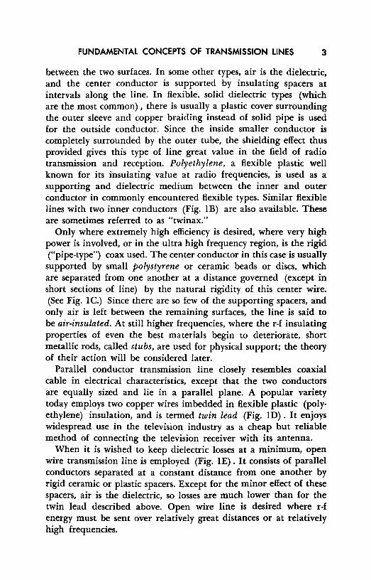
Most r-f lines consist of two conductors separated by an insulating medium, called a dielectric. Coaxial cable is a concentric line consisting of a small, round conductor situated at the center of the other conductor, which is a surrounding tube. In solid dielectric types, illustrated at (A) of Fig. I, the middle copper wire is held in place by the dielectric medium, which entirely fills the space
FUNDAMENTAL CONCEPTS OF TRANSMISSION LINES 3
between the two surfaces. In some other types, air is the dielectric, and the center conductor is supported by insulating spacers at intervals along the line. In flexible, solid dielectric types (which are the most common) , there is usually a plastic cover surrounding the outer sleeve and copper braiding instead of solid pipe is used for the outside conductor. Since the inside smaller conductor is completely surrounded by the outer tube, the shielding effect thus provided gives this type of line great value in the field of radio transmission and reception. Polyethylene, a flexible plastic well known for its insulating value at radio frequencies, is used as a supporting and dielectric medium between the inner and outer conductor in commonly encountered flexible types. Similar flexible lines with two inner conductors (Fig. lB) are also available. These are sometimes referred to as "twinax."
Only where extremely high efficiency is desired, where very high power is involved, or in the ultra high frequency region, is the rigid ("pipe-type") coax used. The center conductor in this case is usually supported by small polystY,rene or ceramic beads or discs, which are separated from one another at a distance governed (except in short sections of line) by the natural rigidity of this center wire. (See Fig. IC.) Since there are so few of the supporting spacers, and only air is left between the remaining surfaces, the line is said to be air-insulated. At still higher frequencies, where the r-f insulating properties of even the best materials begin to deteriorate, short metallic rods, called stubs, are used for physical support; the theory of their action will be considered later.
Parallel conductor transmission line closely resembles coaxial cable in electrical characteristics, except that the two conductors are equally sized and lie in a parallel plane. A popular variety today employs two copper wires imbedded in flexible plastic (polyethylene) insulation, and is termed twin lead (Fig. ID) . It enjoys widespread use in the television industry as a cheap but reliable method of connecting the television receiver with its antenna.
When it is wished to keep dielectric losses at a minimum, open wire transmission line is employed (Fig. IE) . It consists of parallel conductors separated at a constant distance from one another by rigid ceramic or plastic spacers. Except for the minor effect of these spacers, air is the dielectric, so losses are much lower than for the twin lead described above. Open wire line is desired where r-f energy must be sent over relatively great distances or at relatively high frequencies.
4 R-F TRANSMISSION LINES
In the presence of a large amount of external noise, or where radiation is to be kept to a minimum, a shielded two-conductor transmission line is sometimes used (Fig. IF). This is not to be confused with coaxial line. It is similar to twinax (Fig. IB). However, instead of both conductors being imbedded in a single cylinder of dielectric, these conductors are separately insulated and "airspaced" by a cord of polyethylene twisted between them. As with twinax, the metal braid helps to prevent radiation from entering or leaving the transmission line. It is more expensive than other forms of parallel wire line.
Hollow dielectric parallel conductor transmission line is most useful in seaside areas where salt spray coats the plastic dielectric. Under these conditions most types of parallel conductor lines would be shorted by the salt residue. The hollow dielectric line, however, greatly increases the leakage path from one conductor to another due to the lengthened surface of its cylindrical configuration (Fig. IG).
Twisted lead (like lampcord) , due to its high dielectric losses, finds little practical use at radio frequencies (Fig. IH). Its use is confined to high signal strength areas and to where short lines are sufficient.
As was pointed out, all of the above transmission lines are variations of two basic types - coaxial and parallel conductor. Even these basic types, however, emanate from a fundamental theory common to all r-f transmission lines. For the purpose of the analysis and explanation of this theory, we will deal with the parallel conductor variety.
3. Lumped and Distributed Constants
Since transmission lines consist of a very special arrangement of conductors, they possess certain properties dictated by their electrical as well as their physical makeup. For instance, all conductors have resistance, and this property is not excluded from transmission lines. Parallel copper wires may have resistance in the order of a fraction of an ohm per hundred feet, but it is a factor that must be considered, since it offers a tangible hindrance to the flow of current. Since this resistance is distributed over the entire length of the line, each unit length (inch, foot, yard, etc.) possesses a certain resistance. In an attempt to visualize this distributed resistance schematically, it is a practice to lump or gather it in one
FUNDAMENTAL CONCEPTS OF TRANSMISSION LINES 5
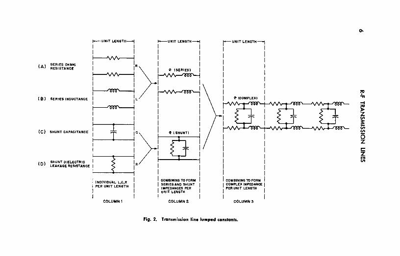
place, while considering the remaining part of the unit length as a perfect conductor (Fig. 2A) . As long as the length of line is considered as a whole, its lumped resistance indicates its true characteristic.
Similarly, magnetic lines of force surround all conductors that carry an electric current. This is a property of inductance. For de and low frequencies a pair of wires is not normally thought of as having appreciable inductance, since its inductive effect on the passing current is very small.
At radio frequencies this inductance is no greater, but its efject on passing current is so magnified (because of the increased inductive reactance) that it can no longer be ignored. We must, therefore, consider each unit length of wire as possessing an inductance lumped in one place (Fig. 2B) as we do in considering resistance.
Any two conductors separated by an insulator form a capacitor. The actual capacitance between the two wires of a transmission line will vary with the spacing and wire size; schematically, it can be shown as lumped (Fig. 2C) . Any material chosen as the dielectric between the two wires must have some leakage resistance (Fig. 2D) ; it will vary with the material chosen, air being a near-perfect insulator. Shunt capacitance and insulator or dielectric leakage are thought of as being in parallel, and therefore when lumped are represented in that manner. In addition, since resistance and inductance exist in the same unit length of wire, they may be considered as an R-L impedance. (See Fig. 2, column 2.) Because we are concerned with the same unit length of wire, whether referring to series inductance and resistance or to parallel capacitance and resistance, we may combine these constants to form a complex impedance per unit length (Fig. 2, column 3) . Note that each wire contains only half of the total series impedance per unit length.
4. Variations of Constants
The impedances just described are not constant but vary with frequency. The resistance of a wire has its d-c value only when the distribution of current is uniform throughout the cross section area. The resistance of a wire is:
R=p~
where p = resistivity, in ohms per circular mil foot
(Al SERIES OHMIC RESISTANCE
!--UNIT LENGTH-----! t---UNIT LENGTH----!
I I I I I I I I 1-------'\/v'\, I I I IR I I
f---'W'v-----1 ~ l I I I ~ I I
I I >I r (SERIES! I
I ~ (Bl SERIES INDUCTANCE I IL I I ~ I I 1 I I I I I I I I I I I I
(Cl SHUNTCAPACITANCE : I :c>lcrur(SHUNTl I I I I I I I I I I I I I
( l SHUNT OIELECTRICtD I D LEAKAGE RESISTANCE I IR I I
I I I I I I COMBINING TO FORM I
INDIVIDUAL L,C,R I I SERIES ANO SHUNT I j PER UNIT LENGTH IMPEDANCES PER I I I UNIT LENGTH I I I I I
COLUMN 1 COLUMN 2
J UNIT LENGTH--j
I I I I I I I I I I I I I I I I I r tCOMPLEXl I
,........rll'lOI
I COMBINING TO FORM I COMPLEX IMPEDANCE I I PER UNIT LENGTH I
I I COLUMN 3
Fig. 2. Transmission line lumped constants.
0,.
~ .,, -I
~ z en ~ en en 5 z r-z ~
FUNDAMENTAL CONCEPTS OF TRANSMISSION LINES 7
LINES OF FORCE INSIDE a OUTSIDE
OF CONDUCTOR
(A)
OUTER SURFACE
oo"'~
ELECTRON DISTRIBUTION
AT ZERO FREQUENCY
(8)
Fig. 3. Skin effect.
and: , = length of conductor (in feet)
A V ELECTRON
DISTRIBUTION AT RAOIO
FREQUENCIES
(C)
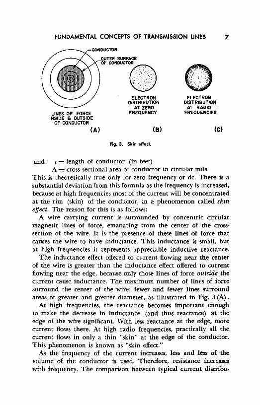
A = cross sectional ;i.rea of conductor in circular mils This is theoretically true only for zero frequency or de. There is a substantial deviation from this formula as the frequency is increased, because at high frequencies most of the current will be concentrated at the rim (skin) of the conductor, in a phenomenon called skin effect. The reason for this is as follows:
A wire carrying current is surrounded by concentric circular magnetic lines of force, emanating from the center of the crosssection of the wire. It is the presence of these lines of force that causes the wire to have inductance. This inductance is small, but at high frequencies it represents appreciable inductive reactance.
The inductance effect offered to current flowing near the center of the wire is greater than the inductance effect offered to current flowing near the edge, because only those lines of force outside the current cause inductance. The maximum number of lines of force surround the center of the wire; fewer and fewer lines surround areas of greater and greater diameter, as illustrated in Fig. 3 (A) .
At high frequencies, the reactance becomes important enough to make the decrease in inductance (and thus reactance) at the edge of the wire significant. With less reactance at the edge, more current flows there. At high radio frequencies, practically all the current flows in only a thin "skin" at the edge of the conductor. This phenomenon is known as "skin effect."
As the frequency of the current increases, less and less of the volume of the conductor is used. Therefore, resistance increases with frequency. The comparison between typical current distribu-

8 R-F TRANSMISSION LINES
tion for direct current (B) and high frequency current (C) is shown in Fig. 3.
As explained above, current flowing near the edge of the conductor encounters less inductance. Thus, flow of current in the skin causes inductance to decrease as frequency increases. However, for the normal range of radio frequencies, the inductance change is very small and can be neglected.
Shunt dielectric leakage increases with frequency, and must be known when calculating line losses. Any variations in shunt capacitance with frequency are usually too small to be of consequence.
5. Review Questions
(1) In one sentence define the function of a transmission line. (2) What are the two main types of r-f transmission line? (3) Why is the term "air-insulated" applied to some types of line? (4) What is the main advantage of coax cable, in preference to parallel
conductor Fne? (5) What is meant by "lumped constants"? (6) How is the theory of lumped constants applied to the equivalent schematic
representation of transmission lines? (7) How does "skin effect" affect the total resistance of a line at any given
frequency? (8) Does skin effect affect the flow of direct current? (9) Does the flux density differential (which is responsible for skin effect)
also exist at zero frequency? (10) At high radio frequency, in what region of the conductor does the current
flow? (II) At high radio frequency, how will the conducting qualities of a hollow
conductor compare with those of a solid conductor? Why? (12) If the cross-sectional area of a given conductor is doubled, how will the
d-c resistance per unit length vary? (13) If a given wire 1 inch in diameter has a d-c resistance of .01 ohm per
meter, what d-c resistance will a wire 2 inches in diameter have if both wires are made of the same material and are the same length?
(14) In general, how do the losses on a transmission line vary as the frequency is increased?

Chapter 2
TRANSMISSION LINE OPERATION AND CHARACTERISTICS
6. Wavelength and Velocity
Since electromagnetic waves travel in a given direction at a finite velocity, they must cover a certain linear distance during the time of one cycle. The distance covered in this time is called the wavelength, and is usually expressed in the metric system; it is assigned the symbol A. The velocity of this wave equals the distance covered during one cycle (A) divided by the time (T) of one cycle:
Velocity
Remembering that l_ _ f T
A (V) = T
then also (V) = A/ This fundamental equation points out an interesting fact: the velocity of a wave is governed solely by the properties of the medium through which it is transmitted and in no way is affected by the frequency or the wavelength. The velocity of an electromagnetic wave in any medium is approximately:
V ( d) 3 X 10⁸ meters per second
meters per secon = -yk where k = the dielectric constant of the medium; k = 1 for air.
So far, we have discussed transmission lines in a general way. R-f lines, as opposed to those carrying lower-frequency current, have some peculiarities all their own. They arise from the fact that
9
10 R-F TRANSMISSION LINES
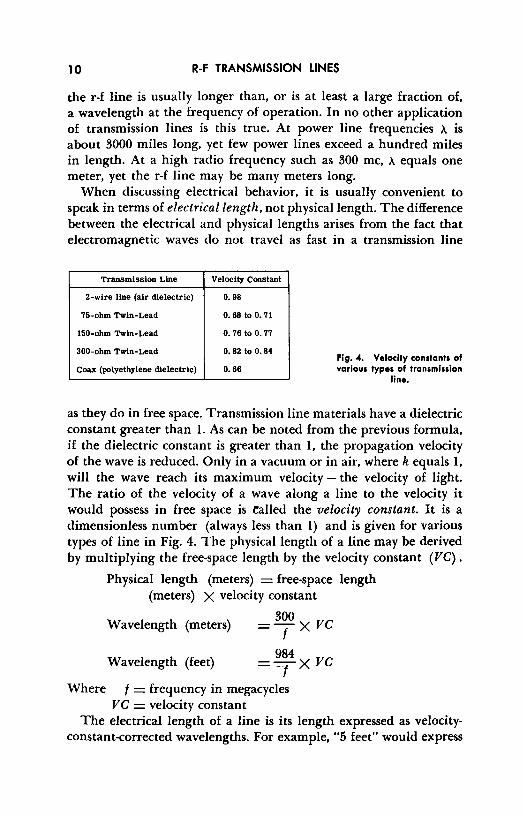
the r-f line is usually longer than, or is at least a large fraction of, a wavelength at the frequency of operation. In no other application of transmission lines is this true. At power line frequencies ,\ is about 3000 miles long, yet few power lines exceed a hundred miles in length. At a high radio frequency such as 300 me, ,\ equals one meter, yet the r-f line may be many meters long.
When discussing electrical behavior, it is usually convenient to speak in terms of electrical length, not physical length. The difference between the electrical and physical lengths arises from the fact that electromagnetic waves do not travel as fast in a transmission line
Transmission Line
2-wire line (air dielectric)
75-ohm Twin-Lead
150-ohm Twin-Lead
300-ohm Twin-Lead
Coax (polyethylene dielectric)
Velocity Constant
0.98
o. 68 too. 71
o. 76 too. 77
o. 82 to 0. 84
0.66 Fig. 4. Velocity constants of various types of transmission
line.
as they do in free space. Transmission line materials have a dielectric constant greater than I. As can be noted from the previous formula, if the dielectric constant is greater than 1, the propagation velocity of the wave is reduced. Only in a vacuum or in air, where k equals I, will the wave reach its maximum velocity - the velocity of light. The ratio of the velocity of a wave along a line to the velocity it would possess in free space is ~ailed the velocity constant. It is a dimensionless number (always less than 1) and is given for various types of line in Fig. 4. The physical length of a line may be derived by multiplying the free-space length by the velocity constant (VC).
Physical length (meters) = free-space length (meters) X velocity constant
Wavelength (meters)
Wavelength (feet)
= 3~0 X vc
= ~~4 X vc Where f = frequency in megacycles
VC = velocity constant The electrical length of a line is its length expressed as velocity
constant-corrected wavelengths. For example, "5 feet" would express

TRANSMISSION LINE OPERATION AND CHARACTERISTICS 11
a physical length, while "half-wavelength" would express electrical length.
If a wave in a line has a finite velocity, it must require increasing amounts of time to reach successive points at greater distances from the source of the wave. The action is depicted in Fig. 5, where it is seen that at each point in question (A, B, and C) there exists a separate oscillation created by the travelling wave moving toward the right away from the source (S). Because each of these oscillations is actuated by a single wave front, which requires time to travel from one point to the next, the oscillations will occur at a later
90•
/ ..... , I I
SOURCE POINT A POINT 8 POINT C POINT D
gt• !. ! ! !
,so•~o• @s • • EBo• EBO" e,;800 o• 380" wl8o-s w w a s
270° J 270° I .b.. _____j VECTOR REPRESENTATIONS 4
2>. • I W • CURRENT AT POINT INDICATED i-------4 S • SOURCI! CURRENT AT SAMI! TIMI!
--------!). ------...i ---------->.-----------
Fig. 5. Relation of phases of currents at different points along a transmission line.
time at each point progressively distant from the source. Specifically, by the time the wave has reached point A, and has started an oscillation at that point (commencing at zero degrees), the source vector has advanced 90 degrees. Vector A must then lag behind the source by a phase angle of 90 degrees, or a quarter of a cycle. By the time the wave has reached point B, and started an oscillation at that point (commencing with zero degrees), the source vector has advanced another 90 degrees. Point B vector now lags point A vector by 90 degrees and the source by 180 degrees. By the time the

12 R-F TRANSMISSION LINES
wave has finally reached point C, the source, point A, and point B vectors have revolved another 90 degrees, placing C vector 270 degrees, B vector 180 degrees, and A vector 90 degrees lagging phase angle from the source reference vector.
The phase shift introduced by travel of a wave from the source to any physical point along the line is a function of two things: the propagation velocity on the line, and the distance of that point from the source. In general, however, any wave travelling down any line will become more lagging in phase as the distance increases from the source of that wave.
Note that if a point (D) is included in Fig. 5 and is considered with the above discussion, the difference in phase between this point and the source is exactly 360 degrees, one cycle, or 271' radians. If the distance from the source to point D is the distance covered by this wave during the time its vector has lagged or rotated one complete cycle, or 271' radians, then this distance is also one wavelength - since one wavelength has been previously described as the distance covered by the wave during the time of one cycle. A wavelength may also be defined as the distance between points whose voltages (or currents) differ in phase by one cycle, or 271' radians.
The rate of change of phase of the wave as it travels down the line can be expressed by the number of radians (or degrees) the phase changes per unit length of the line. The phase change per unit length is indicated by the symbol f3 (Greek letter beta) . It can be expressed in any convenient units, such as radians per foot, degrees per yard, etc., but it naturally simplifies any calculations to express f3 in units consistent with other measurements involved.
We have already said that a wavelength is the distance in which the phase changes by a whole cycle; a whole cycle is equivalent to 271' radians or 360 degrees. Thus wavelength multiplied by phase change per unit length must equal the number of radians or degrees in a full cycle.
If /3 is in radians per unit length and ,\ is in the same length units as /3, then:
,\(3 = 271' radians

TRANSMISSION LINE OPERATION AND CHARACTERISTICS 13
1£ f3 is in degrees per unit length and >,, is in the same length units as {3, then:
>,,f3 = 360°
360 >,, =13
360 /3=A
7. Characteristic Impedance
Let us view the action of a wave as it progresses from the place where it enters the line (called a source) to the place where it is to be used (called a load).
Imagine a line of infinite length represented by a chain of lumped impedances as shown in Fig 6 (A). Electromagnetic energy emitted from the generator will be propagated down the line. Some of the original current leaving the generator (labeled / 0) will be diverted through the first shunt impedance at point a and return to the generator. Obviously, this shunt current (/1 ) will detract from the total current available to continue down the line; the current left will be 10 - / 1 • Farther on at b, after shunting current / 2 has detracted from the remaining curent, only / 0 - (/1 +12) is left to continue down the line; at c, only / 0 - (/1 +12 +18) is left. It can be shown that, as the wave progresses away from the generator, the shunting currents increase and finally equal / 0 • At this point there is no energy left to continue. The process is indicated graphically in Fig. 6 (B) . Note that the decline is gradual. This is what would happen in an actual line of infinite length, since the constants are not lumped as shown, but are distributed throughout the entire length of the line. The voltage decreases gradually in much the same manner, due to the series impedance.
Since there is current flowing at the source, the generator connected to this infinitely long line must "see" a definite impedance. The ratio of voltage to current of the wave travelling away from the generator establishes this impedance. It is called the characteristic impedance (or surge impedance) of the line, and is given the symbol Z0 •
As was stated, the relationship of E to I on an infinitely long line is its characteristic impedance.

14
(A)
(B)
(C)
(D)
R-F TRANSMISSION LINES
lo·U,+Iz)- C
DISTANCE FROM GENERATOR -
·} Y• ~g•+l)Z • ~!b o•fs• b•ic • <JC
SIMPLIFIED REPRESENTATION OF TRANSMISSION AT HIGH FREQUENCIES
Fig. 6. Characteristic impedance.
TO INrtNITY-

TRANSMISSION LINE OPERATION AND CHARACTERISTICS 15
Z _ E, where E, = voltage across infinite line 0
- I, I, = current into infinite line The characteristic impedance of a transmission line can also be
shown to be as indicated by the following formula:
Z0 =v/f where Z 0 is characteristic impedance in ohms
Za is series impedance per unit length (ohms) Y is shunt admittance per unit length (mhos)
The factors in Z0 and Y are illustrated in Fig. 6 (C). Z 0 is developed from R and L in the well-known relation:
Za = ✓ R2+w2L2
The shunt leakage resistance and capacitance are effectively in parallel. For this reason, it is simplest to combine them as reciprocals. The reciprocal of the leakage resistance is conductance (g) and the reciprocal of capacitive reactance is susceptance (b). These two combine to form the total admittance, Y, which is used in the formula above, as follows:
Y=-Jg2+b2 But b is the reciprocal of X 0 , and is thus equal to wC
thus Y=y g2
,---::::;..:;.===w:;;,21'="~'!c"2 and
g +w2 2
R and g both increase with frequency. However, w2 increases so much faster that, for practical r-f lines, at all but the lowest radio frequencies R and g become negligible, with the line assumed to be as in Fig. 6 (D) . The expression for characteristic impedance is then simplified as follows:
L Zo=c It should be noted that, since L and C are substantially constant
(for all but very low radio frequencies), Z0 must also be constant. Thus the conclusion: for a given geometric cross-section and insulating material, characteristic impedance is constant for all radio _frequencies. Measuring the inductance and capacitance of a line is not necessary for determining Z0 • By substituting formulas for inductance and for capacitance (in terms of the line's actual construction) and substituting for L and C in the above formula, we may deduce for parallel conductor line:
16
800
750
700
300
250
200
15 0
R-F TRANSMISSION LINES
1.5 2 2.5 3 4 5 6 7 8 9 IO
SPACING BETWEEN CONDUCTORS (INCHES)
SIZE OF
WIRE USED
DIAM. OF
USING USED
150
'" u z 120
"' C
lf 110
~ vi
u ~ 100
~9 ir '" ::; "' "' "' :i: u
.15 .2 .25 .3 .4 .5 .6 .7 .8 .9 1.0
INNER OIAM. OF OUTER CONDUCTOR (INCHES)
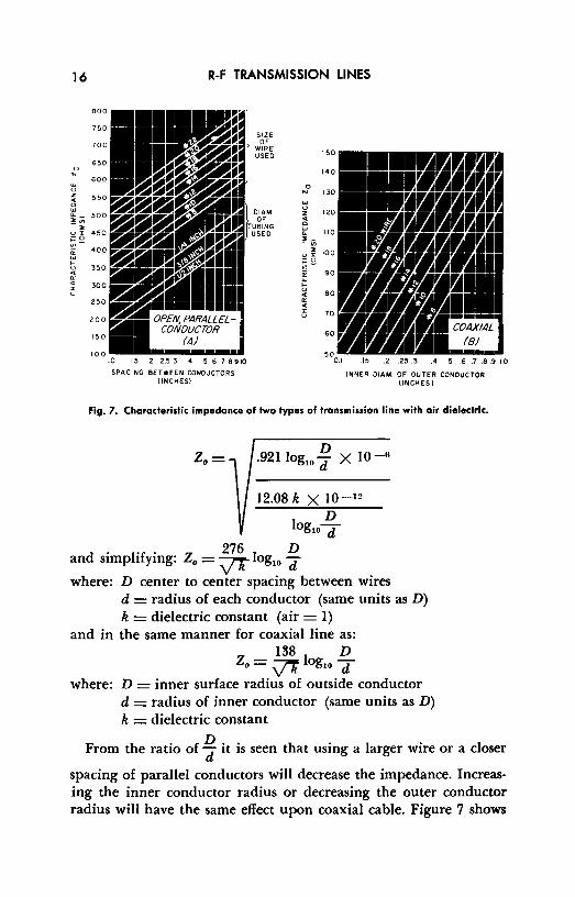
Fig. 7. Characteristic impedance of two types of transmission line with air dielectric.
D .921 log10 d X IO - 6
12.08 k X IO - 12
D log107
d . l"f . Z 276 l D an s1mp 1 ymg: 0 = -:;::Tr og10 7 where: D center to center spacing between wires
d = radius of each conductor (same units as D) k = dielectric constant (air= 1)
and in the same manner for coaxial line as: 138 D
Zo=;::rtlog107
where: D = inner surface radius of outside conductor d = radius of inner conductor (same units as D) k = dielectric constant
From the ratio of ~ it is seen that using a larger wire or a closer
spacing of parallel conductors will decrease the impedance. Increasing the inner conductor radius or decreasing the outer conductor radius will have the same effect upon coaxial cable. Figure 7 shows

TRANSMISSION LINE OPERATION AND CHARACTERISTICS 17
how wire size and spacing affect the impedance of parallel conductor and coaxial line respectively.
The dielectric constant (k) of most materials varies with frequency. However, for materials used for insulation in practical transmission lines (notably polyethylene), k is substantially constant over the entire r-f range. Thus Z0 for a transmission line of given cross-section is constant.
At this point the reader may question the practicality of discussing an infinitely long line, which obviously does not exist in a physical sense. Under certain circumstances, however, the wave reaching the end of a line is unable to distinguish between this end and an infinite extension of the line; the line as a whole has the charac• teristics of an infinite line. Let us examine the reasons for this.
8. Line Termination
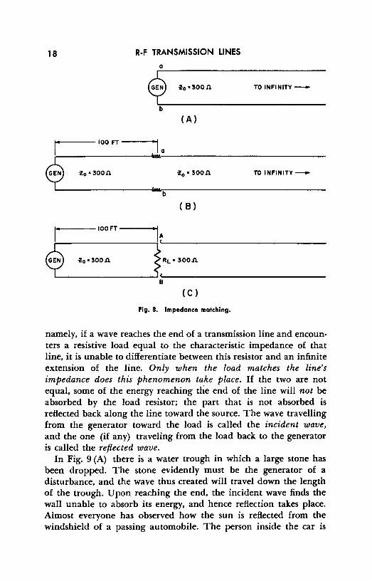
Assume the generator in Fig. 8 (A) is looking into an infinitely long line of 300 ohms characteristic impedance (for simplicity lumped constants have not been shown). If we break the connection at a and b and insert a section of line (say 100 feet) between a and b and the generator, it will not make any difference to the generator, since a finite distance added to an infinite distance is still an infinite distance. The new l 00-foot insertion is shown in Fig. 8 (B) .
It is agreed that the generator will still "see" a 300-ohm impedance - even with the 100-foot piece of line inserted. In addition, however, when the electrons bounding down the line reach a and b, they will also see 300 ohms, the Z0 of an infinite line. This is logical because it corresponds to the Z0 the generator saw when it was located at a and b. Now if we were to again break the connection at a and b, but this time insert a 300-ohm resistor (called the load resistance) in place of the infinitely long line (Fig SC) , the electrons reaching this resistor would not find conditions altered in the least; in fact, they would interpret this 300-ohm resistor as being the same infinitely long 300-ohm line - even though it is physically quite different. Under these conditions it is said that there is an impedance match betwen the line and load.
9. Reflections
It would be well for the reader to reread the previous paragraph, since it contains one of the most important concepts in this book;
18 R-F TRANSMISSION LINES
a
~o •300.n TO INFINITY-
(A)
1· 100 FT · I a
$ ~o • 300.n :, ~o • 300.n TO INFINITY-
( B)
I. IOOFT •1A
$ ~o • 300.n ~-,· ,.,,, B
(C)
Fig. 8. Impedance matching.
namely, if a wave reaches the end of a transmission line and encoun• ters a resistive load equal to the characteristic impedance of that line, it is unable to differentiate between this resistor and an infinite extension of the line. Only when the load matches the line's impedance does this phenomenon take place. If the two are not equal, some of the energy reaching the end of the line will not be absorbed by the load resistor; the part that is not absorbed is reflected back along the line toward the source. The wave travelling from the generator toward the load is called the incident wave, and the one (if any) traveling from the load back to the generator is called the refiected wave.
In Fig. 9 (A) there is a water trough in which a large stone has been dropped. The stone evidently must be the generator of a disturbance, and the wave thus created will travel down the length of the trough. Upon reaching the end, the incident wave finds the wall unable to absorb its energy, and hence reflection takes place. Almost everyone has observed how the sun is reflected from the windshield of a passing automobile. The person inside the car is
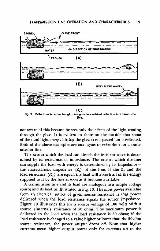
TRANSMISSION LINE OPERATION AND CHARACTERISTICS 19
WATER -+ DIRECTION OF PROPAGATION
TROUGH (A)
,,, __ ------------- ---·--
( B) R1::FLECTED WAVE\
(C) Fig. 9. Reflections in water trough analogous to electrical reflection in transmission
line.
not aware of this because he sees only the effects of the light coming through the glass. It is evident to those on the outside that some of the total light energy hitting the glass is not passed but is reflected. Both of the above examples are analogous to reflections on a transmission line.
The rate at which the load can absorb the incident wave is determined by its resistance, or impedance. The rate at which the line can supply the load with energy is determined by its impedance -the characteristic impedance (Z0 ) of the line. If the Z0 and the load resistance (RL) are equal, the load will absorb all of the energy supplied to it by the line as soon as it becomes available.
A transmission line and its load are analogous to a simple voltage source and its load, as illustrated in Fig. 10. The most power available from an electrical source of given source resistance is that power delivered when the load resistance equals the source impedance. Figure 10 illustrates this for a source voltage of 100 volts with a source (internal) resistance of 50 ohms. The maximum power is delivered to the load when the load resistance is 50 ohms; if the load resistance is changed to a value higher or lower than the 50-ohm source resistance, the power output drops off. Note that higher currents mean higher output power only for currents up to the

20
~-I I I I I I L
R-F TRANSMISSION LINES
LOAD
-./ R I I I-~L ::>
Q.
I I-::>
I 0 .J Ill
I-I-;
50.0.
50 MATCHING LOAD -,,
I - -45 I -I
I I
40
20 30 40 50 60 70 80 90 IOO LOAD RESISTANCE RL, OHMS
SOURCE RESISTANCE Rs • 50 A (CORRESPONDING TO ~o OF LINE)
!!b. 2_ Po !Al (AMPS) (WATTS)
20 1.43 40.8 SAMPLE CALCULATION
30 1.25 46.8 RL • 40A 40 1.11 49.2
TOTAL RESISTANCE•Rs + RL • 50 + 40 • 90A 50 1.0 50
60 .909 49.5 I• .!Q.QY. I.II AMPS 90A
70 .833 48.5 Po• I 2 RL • ll.11) 2 X40 80 .769 47.2 • I.II X I.II X 40 • 49.2 WATTS
90 .714 45 .9
100 .667 44.5
Fig. 10. Relations between load resistance and power output for voltage source of given fixed resistance. Relations are the some for transmission line in which
Zo corresponds to source resistance.
maximum power value; although lower load resistances increase current, they do not absorb as much power.
The same principle applies in a transmission line. The characteristic impedance of the line corresponds to the source resistance, and the resistance of the circuit connected to the end of the line corresponds to the load resistance, RL. The first wave of electrical energy that travels down the line is called the incident wave. If the load resistance equals Z0 , all of the incident energy is absorbed. If not, some energy "bounces back" in what is called a refiected wave.
It may then be said that if there are no reflections on a line the incident wave is the only wave on the line, and the ratio of I to E of that wave is the same at every point on the line. Z 0 is now defined as:
TRANSMISSION LINE OPERATION AND CHARACTERISTICS 21
E, Za=-r; Where: Ei = the voltage of the incident wave
Ii = the current of the incident wave Z0 = the characteristic impedance of the line
This is true for every point on the line, including the load end. It means that the ratio of the amount of current flowing through the line to the value of voltage existing across the line is determined by the Z0 or E/1, when there are no reflections.
The ratio of the amount of current that will flow through the load to the amount of voltage across the load is determined by the load resistance (RL), or ELf IL.
Since the form in which the line can supply energy to the load
is governed by f' and the form in which the load can accept this
power is governed by ;: , it should be clear that if the load is to
absorb all of the power supplied to it by the line, the two ratios must be equal. Therefore, if
E, EL -r;= IL
where EL= voltage across the load IL= current through the load
then Z0 = RL
If, however, RL does not equal Z0 , the ratios oft to ;: will not
be equal and there will be reflection. The magnitude of the reflected wave will be determined by the amount of impedance mismatch, or
the amount by which the ratios of7t and EILdiffer. The magnitude i L
of the reflected wave will always be just large enough to make the
ratio of 7; of the part not reflected just equal to the ratio of 7: of the load resistance. This means that the load will absorb all the incident wave power only when the ratio of voltage to current of that power is numerically equal to the load resistance. If incident wave power possessing any other ratio of E, to I, reaches the load, the correct amounts of I, and E, will be rejected by this load to
make the amount remaining (in the form of-}) just equal to the 1
load resistance.
22 R-F TRANSMISSION LINES
It may be easier to understand the effects in transm1S1on lines if the concept of a "wave" is considered further. A high-frequency pulse, or wave, takes a finite time to travel along the line. Unlike a steady-state voltage or current, it is not necessarily governed by the whole circuit. Rather, for the moment during which the incident wave is first sent down. the line, its energy is "released" from the remainder of the circuit. Its voltage and current are related according to the Z0 of the line, and are not affected by the source and the load. However, when the termination (load) of a line that is not matched is encountered, the incident wave voltage-current relationship is upset, and reflected energy must be released to keep the load voltage and current in proper Ohm's law relation to load resistance. At the same time the reflected wave, as it leaves the load and moves toward the source, must (like the incident wave) maintain a voltage-current ratio equal to Z0 •
The currents and voltages in the line and at the load are governed by basic electrical laws as follows:
a. The vectorial sum of the voltage of the incident wave and the voltage of the reflected wave must equal the load voltage.
b. The ratio of incident voltage to incident current, and the ratio of reflected voltage to reflected current, must both equal Z0 of the line.
c. The ratio of load voltage to load current must equal load resistance.
If all the above conditions are combined and solved mathematically, an expression for the ratio of the reflected wave voltage to the incident wave voltage is obtained. This ratio is known as the reflection coefficient (k). Its value can be calculated in any given case from:
ZL - I RL - I k - .,.2-0 ---; for resistance load: k = R_Z..;;.o __ _ -~+I _.!:_+I
Zo Zo
RL-Zo or: k = R + Z
I, 0
In the simple (and fortunately most common) case in which the load is (or can be considered to be) a pure resistance, k is not a complex quantity, but may be plus or minus. Examination of the above equation shows that when load impedance (resistance) is greater than Z0 , k is positive. When load resistance is less than Z0 ,
k is negative.
TRANSMISSION LINE OPERATION AND CHARACTERISTICS 23
To clarify the above ideas, consider some examples. First, suppose a 300-ohm (Z0) transmission line is terminated in a 300-ohm resistance (load) . Substituting in the equation we obtain:
300 - I 300 0
k= 300 =y=O 300 + I
The zero value of k indicates that there is no reflected wave. Thus the line is matched, because the load resistance equals Z 0 • Next, let us assume that the load resistance for the same line is reduced to 150 ohms:
150 -1 300 0.5 -1
k = ..,.15=0,---- - 0.5 + I 300 + I
-0.5 1.5
I T
Thus the reflected wave is of opposite polarity to the incident wave, and has one-third of its amplitude.
It is this unique control the load has over the action of a line that leads us to state that all calculations involving transmission lines must start at the load end of the line.
In summary, the identifying characteristics of a transmission line operating into a matched resistive load are as follows:
a. At every point on the line current and voltage maintain the same phase relationship with one another.
b. At every point on the line, the ratio of voltage to current is always the same and is numerically equal to the characteristic impedance of the line.
c. Maximum amount of power is transferred from the line to the load.
d. No power is reflected back to the generator.
10. Standing Waves
1£ the line we are discussing is being used to feed r-f power from one place to another, it is natural that we do not want mismatches, since they represent a loss of power in the form of reflections. Let us look deeper into what happens when a wave travels back toward its source.
1£ an incident and a reflected wave both exist on a line, the voltage at any given point along the line is the vector sum of the incident wave and reflected wave voltages at that point. Current at any point

24 R-F TRANSMISSION LINES
I IMPEDANCE
CURVES ARE SHOWN WITHOUT REGARD TO POLARITY
Fig. 11. Conditions olong o line with o short circuit load.
SHORTED LOAD END
is similarly derived. The resulting voltage and current distribution along the line depends upon the magnitude and phase relationship between the incident and reflected waves. If the incident and reflected waves are equal in magnitude and in phase, the resultant wave will be double either individual value. At other points where they are exactly 180 degrees out of phase, they will cancel each other. Points of intermediate values of phase and amplitude will produce a result somewhere between these two values. Since the incident and reflected waves cannot exist independently and their voltage and currents always combine vectorially, we will discuss only resultant voltage or current, which is what is actually present and measurable.
The phase relation between the incident and reflected waves is such that their vectorial sum voltage (and current) varies along the line. If a measuring device is moved along the line, it will show that the voltage rises to a peak value, then falls to a minimum, then rises to a peak again. Maxima and minima of voltage alternate with equal spacings. Current also varies between minimum and maximum values: where the voltage is maximum the current is minimum, and where voltage is minimum the current is maximum. These variations of voltage and current are present in any line in which there is a reflected wave [that is, any line in which the load resistance is not matched (equal to) Z0 ].
A minimum point of voltage or current is called a node. A maximum point of voltage or current is called a loop. Thus a current node is also a voltage loop, and a voltage node is a current loop.

TRANSMISSION LINE OPERATION AND CHARACTERISTICS 25
These variations of voltage and current with physical position along a transmission line are referred to as standing waves. Each successive node is spaced a half wavelength from its predecessor and each successive loop is spaced a half wavelength from its predecessor (allowing for velocity factor). Their actual position in relation to the load end of the line depends on whether the incident wave finds a short or open circuit, or reactive impedance at the load.
Where it is desired to transmit r-f power over a distance with greatest efficiency and economy, standing waves have the following disadvantages:
a. "Copper" losses are very high. Power loss in the conductors is the summation of the I 2R losses at all points along the line. With appreciable standing waves, the high values of current at and near current loops result in a large increase in copper losses over those of a matched line. The increase in power loss at current loops is much greater than the decrease in power loss at current nodes, so the overall copper losses are increased.
b. Dielectric losses are also increased in the same manner. c. Peak voltage at voltage loops is often so high (in transmitter
applications) that special attention must be given to the provision of insulation. In other words, a heavier duty, more expensive, physically heavier, and more bulky transmission line may have to be used, as compared to matched line requirements.
d. As will be further explained presently, a line with standing waves has an input impedance that is very critical with respect to line length. If the length of the line is not just right at a given frequency, it may be difficult to couple power into it from the source.
When reflections occur, it is sometimes helpful to think of the load as the generator of the reflected wave. If the incident wave strikes a short circuit, no power is absorbed by the load and complete reflection of the incident wave takes place, producing standing waves. Because there is zero resistance at the load point, the reflected current will be maximum and will just equal the incident current. The two currents will add vectorially and produce a resultant current double the individual value. It is therefore said that the two currents are in phase at the shorted end of a line. At a distance one-half wavelength from the load (Fig. 11) the incident and reflected currents will again be in phase. The condition is repeated at half-wavelength multiples from the load.
It might be well to mention that in Fig. 11 it is assumed that the voltage and current both vary in sine wave fashion. Since in actual

26 R-F TRANSMISSION LINES
practice we are mostly concerned with magnitude and not polarity, the graph has been simplified by flipping the negative part up so that both parts of the cycle are above the zero axis.
If the load is shorted, not only will there be maximum current but, according to Ohm's Law, the voltage must be essentially zero at this point. Its value may also be explained by noting that the incident wave and reflected wave voltages are of equal value but opposite polarity; therefore, they cancel. This is verified by substituting zero for ZL in the previous formula; k is shown to be - I, thus the reflected wave is of magnitude equal to the incident wave but of opposite polarity. Because this also is repeated at half-wavelength multiples from the load, any point of maximum current is a point of minimum voltage.
As noted in Fig. 11, a point one-quarter wavelength from the load is a point of minimum current and maximum voltage. It is at this point that the voltages are in phase and the currents out of phase; load conditions have been exactly reversed. The same thing is duplicated at odd multiples of a quarter-wavelength from the shorted load. It can then be said that any point of maximum voltage is a point of minimum current.
Note the peculiar shape of the impedance curve. It is at a zero value whenever the voltage is zero and the current maximum; it rises nearly to infinity when the voltage is maximum and the current zero.
The impedance at any point on the line is equal to the ratio of voltage divided by the current. At the shorted load voltage is zero, and therefore so is the ratio E/1. This accounts for the zero impedance across the shorted load. At a point a quarter-wavelength away from the short, the voltage is maximum and the current is zero; the ratio of E/1 is now infinite, and so is the impedance. The impedance thus varies in much the same way as the voltage; that is, their maximum and minimum points are th~ same points on the line, and conditions of impedance and voltage are repeated every half-wavelength and reversed every quarter-wavelength.
It should be remembered that we are expressing line lengths only electrically (half-wavelength, quarter-wavelength, etc.) . If the frequency of operation is changed and the physical line length is not, the whole voltage and current distribution changes accordingly.
If the incident wave strikes an open circuit at the end of the line, as shown in Fig. 12, there can be no current through this near-infinite resistance; only a large voltage may exist. Again, no power will be
TRANSMISSION LINE OPERATION AND CHARACTERISTICS 27
1..). 4
§.). 4
~). 4
~). 4
IMPEDANCE
..! ). 4
_g_). 4
i!o
OPEN CIRCUIT
LOAD
CURVES ARE SHOWN WITHOUT REGARD TO POLARITY
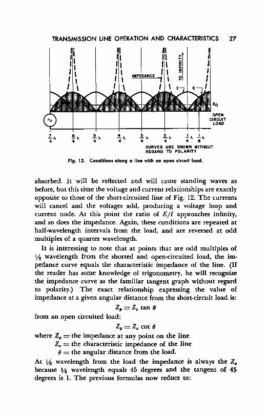
Fig. 12. Conditions along a line with an open circuit load.
absorbed. It will be reflected and will cause standing waves as before, but this time the voltage and current relationships are exactly opposite to those of the short-circuited line of Fig. 12. The currents will cancel and the voltages add, producing a voltage loop and current node. At this point the ratio of E/l approaches infinity, and so does the impedance. Again, these conditions are repeated at half-wavelength intervals from the load, and are reversed at odd multiples of a quarter wavelength.
It is interesting to note that at points that are odd multiples of Ys wavelength from the shorted and open-circuited load, the impedance curve equals the characteristic impedance of the line. (If the reader has some knowledge of trigonometry, he will recognize the impedance curve as the familiar tangent graph without regard to polarity.) The exact relationship expressing the value of impedance at a given angular distance from the short-circuit load is:
Z,=Z0 tan 8 from an open circuited load:
z,, =Z0 cot 8 where z,, = the impedance at any point on the line
Z0 = the characteristic impedance of the line 8 = the angular distance from the load.
At Ys wavelength from the load the impedance is always the Z0
because Ys wavelength equals 45 degrees and the tangent of 45 degrees is 1. The previous formulas now reduce to:
28
and:
R-F TRANSMISSION LINES
z, = Z0 tan (45°) = Z0 (1) =Zo
z, = Z0 cot (45°) = Z0 (1) =Zo
A significant comparison may be made here. Impedance, voltage, and current on an open-ended line are everywhere opposite to the same quantities for a shorted line; that is, where shorted line current is high, open line current is low, and vice versa.
11. Standing Wave Ratio
If the line is matched to the load, no reflections occur. If the line is terminated in either a short or an open, complete reflection occurs, with the incident and reflected waves equal in amplitude. If the line is terminated in some value of resistance other than its characteristic impedance, but not an open or short, only some of the power is.reflected- the remaining power being absorbed by the load. Under these circumstances the power in the reflected wave never equals, and is always less than, the incident wave. Maximum and minimum points of voltage and current are still found, but the maximum points are no longer double the value of the reflected or incident waves, and the minimum points are never zero. The ratio of maximum to minimum voltage or current along any line is called the standing wave ratio. It is also a measure of the ratio of mismatch between line and load, or load and line. A mathematical statement of this is:
SWR = Imai» [min
Em= = Emtn
if RL < Z0, then it can be shown that
SWR=~L
if Z0 < RL, then it can be shown that:
SWR=:L 0
where Imaa, = current at current loop

TRANSMISSION LINE OPERATION AND CHARACTERISTICS 29
Im,n = current at current node Em= = voltage at voltage loop Emtn = voltage at voltage node RL = load resistance in ohms Z0 = characteristic impedance of line in ohms SWR = the standing wave ratio of the line
The standing wave ratio (SWR) is a measure of the mismatch of the line termination. Accordingly, it is tied into the coefficient of reflection, k. The two are related as follows:
SWR=: ±: But the relation between k, Z0, and RL (ZL) was given previously. Substituting the equation for coefficient of reflection in the above equation gives:
1-RL-Zo RL + Z0
Examination of this equation shows how it simplifies for the conditions given, as follows:
Rr, > Z0 :
SWR _ RL + ,; + RL - Zv _ 2 RL _ RL - R..t, + Z0 - 14, + Z0 - 2 Z0 - Z0
R 1, < Z0 :
l + Z0 -RL SWR- RL+Zo -~+z0 +z0 -1\
- l _ Zo - RL - RL + z; - z; + RL RL + Z0
If a certain line possesses a SW R of 5, it means that maximum current or voltage is five times minimum current or voltage. It also means that the Z0 is five times RL or ¼ RL. If Z0 equals RL, the ratio is l: 1, and there are no standing waves. The SWR is always l for a matched line. If the load resistance is less than the Z0, there is a current loop and voltage node at the load; if the load is greater in resistance than the Z0 , a voltage loop and current node exist at the load.
Impedance in general is composed of a resistance and a capacitive or inductive reactance. Up to this point the load of a transmission line has been considered as a pure resistance. Many times the line is terminated in an impedance that, although predominantly resis-
30 R-F TRANSMISSION LINES
P • PARALLEL RESONANT CIRCUIT POINTS S • SERIES RESONANT CIRCUIT POINTS
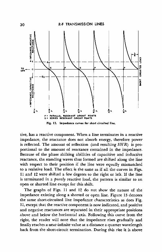
Fig. 13. Impedance curves for short circuited line.
tive, has a reactive component. When a line terminates in a reactive impedance, the reactance does not absorb energy, therefore power is reflected. The amount of reflection (and resulting SWR) is proportional to the amount of reactance contained in the impedance. Because of the phase shifting abilities of capacitive and inductive reactance, the standing waves thus formed are shifted along the line with respect to their position if the line were equally mismatched to a resistive load. The effect is the same as if all the curves in Figs. 11 and 12 were shifted a few degrees to the right or left. If the line is terminated in a purely reactive load, the pattern is similar to an open or shorted line except for this shift.
The graphs of Figs. 11 and 12 do not show the nature of the impedance existing along a shorted or open line. Figure 13 denotes the same short-circuited line impedance characteristics as does Fig. 11, except that the reactive component is now indicated, and positive and negative reactances are separated in their appropriate positions above and below the horizontal axis. Following this curve from the right, the reader will note that the impedance rises gradually and finally reaches a near-infinite value at a distance a quarter wavelength back from the short-circuit termination. During this rise it is above

TRANSMISSION LINE OPERATION AND CHARACTERISTICS 31
J > ;::
~~ cz <>:! :rf~ z"' c"' 0
"' II. ! I
P • PARALLEL RESONANT CIRCUIT POINTS S • SERIES RESONANT CIRCUIT POINTS
.!. ). 4
Fig. 14. Impedance curves for open circuited load.
the zero axis and thus is inductive reactance. At a quarter-wave distance, this near-infinite impedance is resistive in nature; i.e., neither capacitive nor inductive. As distance from the load becomes greater than a quarter wavelength and approaches a half wavelength, the impedance gradually decreases. During the swing, however, it is below the zero line and acts like a capacitor. When it reaches the half-wavelength mark, it is again a resistive impedance, but this time of virtually zero value. The entire process is duplicated during the next half wavelength, varying from zero to maximum inductive reactance, and then a near infinite resistance; from maximum to minimum capacitive reactance, and to zero resistance. The distance along the line back from the load will determine whether it acts like a large or small resistance, or a large or small inductive or capacitive reactance. At multiples of odd eighth wavelengths, it acts as an inductive or capacitive reactance equal to the characteristic impedance. The only limiting factors imposed on the value of impedance at different points are the losses of the line. In the lossless line, the impedance would actually vary from zero to infinity.
Figure 14 shows the impedance curve for a line terminated in an open circuit. The impedance is almost infinitely negative, or capaci-

32 R-F TRANSMISSION LINES
tive, at this point. It decreases to zero a quarter wavelength back from the open end, where it represents a resistance. The curves in Figs. 13 and 14 are exactly the same except that one is displaced 90 degrees (quarter wavelength) from the other. This only corroborates the idea that impedance conditions are reversed every quarter wavelength; a distance a quarter wavelength from an open circuit looks like a short circuit and vice versa. Conditions are duplicated every half wavelength.
12. Input Impedance
So far we have not been overly concerned with the impedance the generator "sees" as it looks into the input end of the line. When the line is matched to its load, the generator sees the Z0 of the line, regardless of its length. Such a line is called a fiat or nonresonant line. If the line is not matched, and standing waves are produced, the impedance the generator "sees" will vary between a maximum and minimum value as the line is made longer or shorter. This impedance is called the input impedance, and is, as always, dependent upon the ratio of E/1 at that point. The amount of possible deviation of input impedance above and below the Z0 depends on the SWR. Because the SWR is infinite when the line is terminated in a short or open circuit, the impedance will vary from near zero to a near-infinite value, depending on the exact line length (in terms of half wavelengths) from the load. All this is to say that if the point we have been discussing in connection with standing wave curves is located at the input of the line, the generator will "see" all the phenomena previously attributed to that point (as shown in Figs. II, 12, 13, and 14). Not only will the input impedance vary with a change in line length, but also with a change in frequency, since in either case the physical length in relation to the electrical length is changed. This means that if the line length is held constant and the frequency is varied, or if the frequency remains the same while the line length is changed, the effect is the same.
Since the input impedance is a function of frequency (and line length) the line is said to be tuned or resonant. Only flat lines with a SWR of I are nonresonant. The effect can be further appreciated by again referring to Fig. 13. At even multiples of a quarter wavelength from the shorted load, the line has a minimum impedance that is purely resistive, like a series resonant circuit. At odd multiples of a quarter wavelength, the impedance is infinite and
TRANSMISSION LINE OPERATION AND CHARACTERISTICS 33
resistive in nature, corresponding to a parallel resonant circuit. The points at which the line exhibits properties of parallel and series resonance are indicated by the letters P and S respectively.
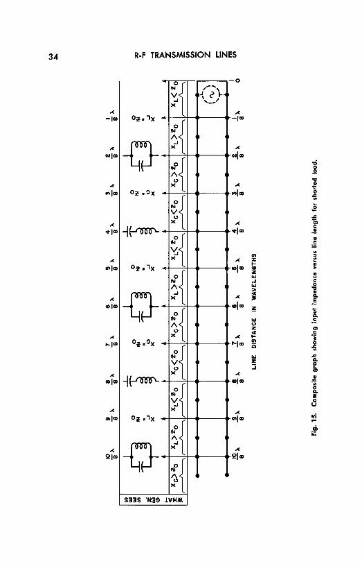
The same sort of conditions exist on an open circuited line (Fig. 14) , but this time the parallel resonant points are even multiples of a quarter wavelength, and series resonant points are odd multiples, away from the load. A composite graph showing variations of input impedance for a short circuited line is contained in Fig. 15, and for open circuited lines in Fig. 16. Perhaps the reader sees the obvious similarity between the two graphs. Every half wavelength the entire cycle of input impedance characteristics repeats itself. The only difference between the shorted and open circuited lines is the point at which the cycle commences. For example, an open circuited line a quarter (2/8) wavelength long has the same input impedance as a shorted line a half wavelength long. Because the reverse also applies, we may say that a shorted line will possess the same input impedance as an open line of any length if the shorted line is longer or shorter than the open line by even multiples of a quarter wavelength. Although losses are greater on a resonant line than on a nonresonant line, it is sometimes more convenient to use a resonant line in practice. This is discussed further in Chap. 3.
13. Line losses
Standing waves can represent a power loss because some of the incident wave power is reflected. Assuming there is no power loss on a mismatched line, the percentage of power absorbed by the load for the same line and source conditions, with a given mismatch ratio, compared to perfect match power is:
percentage of matched-line power absorbed by the load = 2 (SWR)
I+ (SWR)2 X 100
Applying this formula, it can be seen that when the line is matched, the SWR is I, and the percentage of power absorbed by the load is:
2 (I) 1 + (I) 2 X 100 = 100 percent
Every practical transmission line has losses. Although for good highfrequency commercial lines, these losses do not materially affect the characteristic impedance, they nevertheless place a practical limit on the efficiency of any line.
34
,<
-I m
,<
OI )m
,<
on)m
,<
mlm
,<
a,Jm
R-F TRANSMISSION LINES
0
,<
-Jm
,<
°'Im
,<
,.,Im
,<
,..Im
,<
101m
,<
'°Im
,<
""Im
,<
m)m
~{ ,-····\ •{ 2 I-• ,_/
o~. ix
~{ •
-0 ~{ • I
Or • Ox
i{ • I
-1r-"ffl'- ~{ • Or • 1X
~{ • I
-0 ~{ ,. I
or .ox
~{ • • 1r-"ffl'- ~{ • '
0~ .,x
!{ • I
-0 ~{ • S33S 'N39 lltHM
.,, ::c I-Cl) z Ill ..J Ill > ; :!: Ill () z ~ .,, ci
Ill z :i
.. :, :! ii .. u C 0 ,, .. Cl. -~ '5 Cl. -~ 01 C -~ .c .. .c Cl. e 01
-~ 8. E 0 u

TRANSMISSION LINE OPERATION AND CHARACTERISTICS 35
0
0 ,,-, "" A .~~ 2 } ' () ,_..,
>C ;(
oil!.ox Im 0
"" V ' ' () >C ;( ,~ ~{ ' '
ot• ix
... ,.., -ci 1
;( C ,.,,.., .. a. 0
1110
A< ' ' -0 .J
>C
0 Ill A ' ' ()
>C
ot.ox 0
"" t ' I
>C
1~ 0
"" ~ ' ' >C
oil!. ,x 0
"" A< ' I
-0 .J
>C
0
"" A ' ' ()
.. J! ;
;( UI C .,.., ..!! ..
1/1 :§ .. ::c :,
I- :! ;( Cl) .. inlm z > ..,
.J .. .., u C > a
C l :ii: ..<
!: .! colm ;;
::c a. I- .5 Cl)
z UI .., C ..< .J 1 ,..,.., .., -5
z z. .J a. e
UI ..<
.! mlm .; 8. E 0 u
>C
oil!. ox
§{ ' ' ~ff-
..< ,0 OIICD -QI
iL:
;(
2lm
II '
S33S 'N39 .Ll1HM
36 R-F TRANSMISSION LINES
Perhaps the most serious of these losses is radiation. All conductors carrying r-f power tend to act as antennas. The amount of radiation is largely dependent upon the length of the conductor in relation to the wavelength of operation. As mentioned earlier, transmission lines are usually a number of wavelengths long; on this basis they would seem to be good radiators.
We speak of the term "radiation," which applies primarily to a line being used to connect a radio transmitter to its antenna. The object of the antenna system 1s to radiate r-f energy as efficiently as possible. However, it is not desirable that the transmission line itself radiate, because (a) it is normally not as high and "in the clear" as the antenna, and (b) the field from the transmission line interacts with the field from the antenna to produce undesirable directivity effects and losses.
Although we use the term radiation for transmitting applications, the same conditions that produced it also adversely affect reception with the same antenna system. For receiving, the situation is reversed, and what was radiation becomes pickup of unwanted signals, such as man-made noise and other undesired signals the antenna is designed to reject. Therefore, in all discussions, it should be remembered that both radiation and induction losses affect receiving as well as transmitting applications.
Parallel conductor lines contain two wires. If the line has been correctly constructed and installed, the conductors are balanced; i.e., hold the same relationship to ground, are the same size, etc. In balanced line, the currents in the two conductors are equal but flow in opposite directions. Opposing magnetic fields are generated. Theoretically, these opposing fields cancel the total magnetic field surrounding the line, and radiation is eliminated. Unfortunately, this cannot happen completely unless the conductors occupy the same space - an obvious impossibility. Practical lines, however, have little radiation when conductor spacing is kept to .01 wavelength or less. Radiation loss from any two-conductor line varies directly as the square of the frequency and the square of the spacing.
Radiation is proportional to the electromagnetic field intensity; this field is always proportional to the square of the RMS current in the conductors. In the presence of standing waves, the current will be much greater in certain places than would exist on a matched or flat line. Radiation power losses can therefore be expected to increase as the SWR increases.
TRANSMISSION LINE OPERATION AND CHARACTERISTICS 37
Even if most of the overall magnetic field surrounding a line is canceled by proximity of the conductors, the constituent lines of force extend for a significant distance from each conductor. If these lines happen to cut a nearby conducting object, and power is dissipated in that object, it must be supplied by the line. This form of power loss is known as induction loss. To keep induction losses to a minimum, parallel conductor lines are always kept as far away from conducting objetts as possible.
The construction of coaxial lines is such that, when these lines are properly used, losses through radiation and induction can be greatly reduced, compared to parallel conductor types. This is possible because:
a. The conductors are concentric. The fields developed by the two conductors occupy the same position in space, and thus nearly perfect cancellation takes place.
b. The receiver, or other load device, to which power is delivered, is connected to the line in such a way that currents in the shield cannot enter the load. Ordinarily, this is accomplished by connecting the shield to a ground potential point oii the load, which is also connected to earth ground. Thus, although radiation and pickup currents are still present in the shield conductor, they cannot couple to the load and, having a direct ground return, dissipate little power. (In radio systems the source always works against ground.)
Conductor resistance is an important source of power loss in a transmission line. It is often called l 1R or copper loss. The lost power is always dissipated in the form of heat. Since skin effect will only add to the natural resistance of the conductor, a rise in frequency will increase conductor losses. The impedance characteristic of the line will also affect the conductor loss. Specifically, conductor power loss will vary inversely as the square of Z0 , because as Z0 decreases the current for a given power transfer must increase; and, for any conductor with a given resistance, the power dissipation rises with a rise in current.
Dielectic leakage is always responsible for some power loss. It also manifests itself in the form of heat, but rises with an increase in frequency. Of course, the quality of dielectric has a considerable bearing on the loss at any frequency. The heat loss in the dielectric varies directly as does Z0 ; it is the voltage, which va!ies directly as does Z 01 that is the determining factor in shunt dielectric conduction for a given line.

38 R-F TRANSMISSION LINES
14. Review Questions
(1) What is the relationship between the frequency and the period of a given oscillation?
(2) Why is the electrical and not the physical length of a transmission line most important in line calculations?
(3) How does the phase angle compare on a line at different distances from the generator?
(4) At 2-½ wavelengths from the generator, what is the phase angle of a traveling wave at a given instant with reference to the generator?
(5) In actual transmission lines, are constants lumped or distributed? (6) What is the physical length in feet of one wavelength on a line possessing
a velocity constant of .75 and operating at a frequency of 300 me? (7) What is the physical length in meters of the line in the above problem? (8) What is the characteristic impedance of a line at a given point where the
voltage is 58 volts and the current is 0.29 amperes? (9) What is the characteristic impedance of a line whose shunt admittance
per unit length is 0.04 mhos and whose series impedance per unit length is 400 ohms?
(10) Why is it that at high frequencies we need consider only the inductance and capacitance per unit length of a line when calculating its characteristic impedance?
(11) What is the characteristic impedance of a parallel conductor transmission line whose center-to-center spacing between wires is one inch, the radius of each conductor 40.3 thousandths of an inch, and the dielectric constant is 0.9?
(12) What is the characteristic impedance of a coaxial cable when the inner surface radius of the outside conductor is 0.125 inches, the radius of the inner conductor is .015 inch, and the dielectric constant is 0.66?

Chapter 3
APPLICATIONS OF TRANSMISSION LINES
Transmission lines are most noted for their use as carriers of r-f power. Typically, they are employed as a connection link between the transmitter and its antenna, or antenna and receiver; as an interstage coupling device; or for connecting studio and transmitter.
15. The Half-Wavelength Line
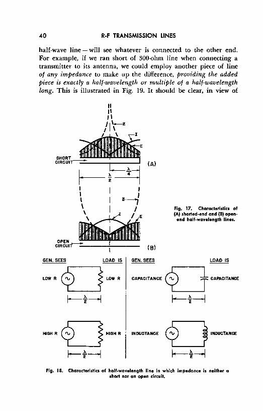
Let us re-examine the voltage, current, and impedance relationship on a shorted line a half-wavelength long, as shown in Fig. 17 (A) . The shorted end of the line has minimum voltage and impedance, and maximum current. Conditions are reversed a quarter wavelength back, but at the generator end a half wavelength away, conditions are duplicated; the generator also "sees" a short. In Fig. 17 (B) the end of the line is an open circuit and the generator also sees an open circuit. In either case the half-wavelength line has caused the source to see whatever load conditions might exist. The idea may be carried further, as in Fig. 18, where it is apparent that the generator will see a resistance if the load is a resistance. Even if the load is a capacitor, the generator, due to a capacitor's current-leading characteristics, will see a capacitive reactance equal to the reactance of the capacitive load; if the load is a coil, the generator will see an inductive reactance equal to the reactance of the coil.
The statement may be broadened to say that anything looking into one end of the half-wavelength line - or any multiple of a
39
40 R-F TRANSMISSION LINES
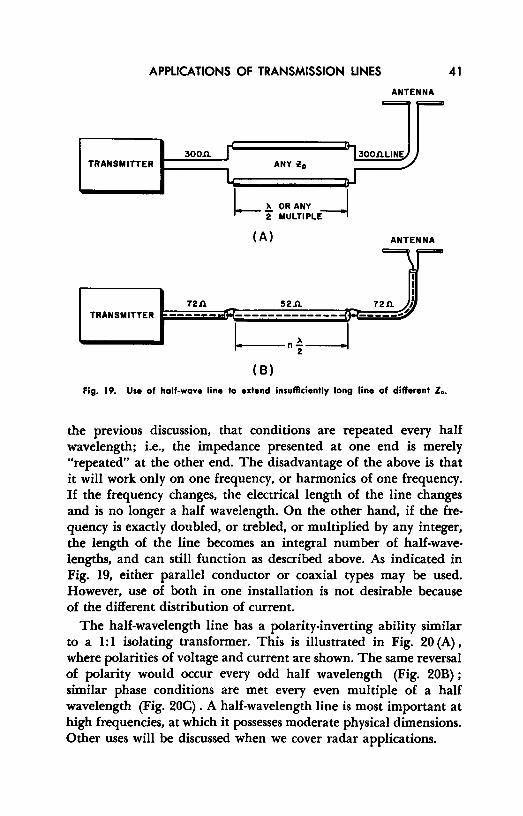
half-wave line - will see whatever is connected to the other end. For example, if we ran short of 300-ohm line when connecting a transmitter to its antenna, we could employ another piece of line of any impedance to make up the difference, providing the added piece is exactly a half-wavelength or multiple of a half-wavelength long. This is illustrated in Fig. 19. It should be clear, in view of
(A)
(B)
GEN.SEES LOAD IS GEN.SEES
Fig. 17. Characteristics af (A) shorted-end and (BJ open
end half-wavelength lines.
LOAD IS
CAMC"A'CEUCAMOTA"°'
1--½--j
""". Li """. 1-½---l
Fig. 18. Characteristics of half-wavelength line In which impedance is neither a short nor an open circuit.
APPLICATIONS OF TRANSMISSION LINES 41
ANTENNA
300.'1. 300.'1.LINE TRANSMITTER -----. ANY ~o
'--). OR ANY I 2 MULTIPLE---!
(A) ANTENNA
72.n TRANSMITTER
( B)
Fig. 19. Use of half-wave line to extend insufficiently long line af different z •.
the previous discussion, that conditions are repeated every half wavelength; i.e., the impedance presented at one end is merely "repeated" at the other end. The disadvantage of the above is that it will work only on one frequency, or harmonics of one frequency. If the frequency changes, the electrical length of the line changes and is no longer a half wavelength. On the other hand, if the frequency is exactly doubled, or trebled, or multiplied by any integer, the length of the line becomes an integral number of half-wavelengths, and can still function as described above. As indicated in Fig. 19, either parallel conductor or coaxial types may be used. However, use of both in one installation is not desirable because of the different distribution of current.
The half-wavelength line has a polarity-inverting ability similar to a 1: 1 isolating transformer. This is illustrated in Fig. 20 (A) , where polarities of voltage and current are shown. The same reversal of polarity would occur every odd half wavelength (Fig. 20B) ; similar phase conditions are met every even multiple of a half wavelength (Fig. 20C) . A half-wavelength line is most important at high frequencies, at which it possesses moderate physical dimensions. Other uses will be discussed when we cover radar applications.

42 R-F TRANSMISSION LINES
+E~OI
~-E
~ -E~--
PHASE REVERSAL
(A)
1• t ., +Er----. I OI~-~....,_-~"'1,;.:----::;.,,,C.-----::..,j"!!=--~.:::---31
Fig. 20. Polarities on half-wavelength lines and multiples af half-wave lines.
16. The Quarter-Wavelength Line
In many ways the quarter-wavelength line is the reverse of the half-wavelength line. In Fig. 21 (A) the quarter-wavelength line segment has a short circuit at one end, but this time the generator "sees" an open circuit, not a short. In Fig. 21 (B) the quarter-wavelength line has an open circuit at the load end, and the generator sees a short. Whereas a half-wavelength line "repeated" the load impedance to the source, a quarter-wavelength line has the power to invert the load impedance. Thus a low impedance at one end of the quarter-wavelength line looks like a high impedance at the other end. The same thing happens if the line is an odd multiple of a quarter wavelength in length. Because of the impedance-inverting property, we call a quarter-wavelength line an impedance trans/ ormer_: it may be used, among other things, as an impedance

APPLICATIONS OF TRANSMISSION LINES
I
'<i! \
\.
" "
SHORTED OUARTER WAVELENGTH LINE
(A)
/
I ~/ I
I E
GENERATO._R_S_E_ES _____ O_P~
SHORT CIRCUIT CIRUIT
OPEN OUARTER WAVELENGTH LINE
(B)
Pig. 21. Conditions on a quarter-wave line section.
43
matching device. Below the vhf region, a quarter wavelength is a number of feet (at 14 me it is approximately 16 feet) and is only useful where there is sufficient room for its application.
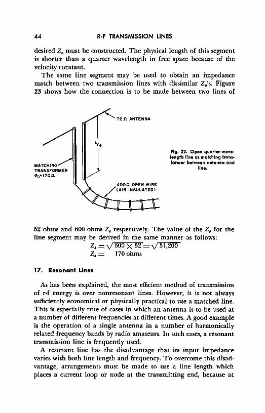
A dipole antenna (at resonance) has a center impedance of 72 ohms, but this is not necessarily the most desirable impedance for the connecting transmission line. The line, for example, might well be of the 400-ohm open wire variety. Now if we connect a quarter wavelength piece of transmission line between the 72-ohm antenna and the 400-ohm line, and if we make this quarter wevelength segment a particular characteristic impedance, the 72-ohm antenna will "see" 72 ohms when looking into the segment, while the 400-ohm line will "see" 400 ohms when looking into the other end. The arrangement is shown in Fig. 22. The value of Z0 for this matching segment may be calculated from:
z. = V 400 X 72 = V 28,800 Z8 = 170ohms
Where Z, Required characteristic impedance of quarter-wavelength matching section; it is always equal to the geometric mean of the two impedances to be matched.
In practice one would choose the commercially available type of line with the nearest Z0 , which in this case is 150-ohm twin lead. Otherwise, sufficient open wire line of proper dimensions for the
44 R-F TRANSMISSION LINES
desired Z0 must be constructed. The physical length of this segment is shorter than a quarter wavelength in free space because of the velocity constant.
The same line segment may be used to obtain an impedance match between two transmission lines with dissimilar Z0 's. Figure 23 shows how the connection is to be made between two lines of
MATCHING TRANSFORM ER ~o• 110.n.
400A OPEN WIRE /<AIR INSULATED)
Fig. 22. Open quarter-wavelength line as matching transformer between antenna and
line.
52 ohms and 600 ohms Z0 respectively. The value of the Z0 for the line segment may be derived in the same manner as follows:
Z8 = V 600 X 52 =V 31,200 z. = 170ohms
17. Resonant Lines
As has been explained, the most efficient method of transmission of r-f energy is over nonresonant lines. However, it is not always sufficiently economical or physically practical to use a matched line. This is especially true of cases in which an antenna is to be used at a number of different frequencies at different times. A good example is the operation of a single antenna in a number of harmonically related frequency bands by radio amateurs. In such cases, a resonant transmission line is frequently used.
A resonant line has the disadvantage that its input impedance varies with both line length and frequency. To overcome this disadvantage, arrangements must be made to use a line length which places a current loop or node at the transmitting end, because at

APPLICATIONS OF TRANSMISSION LINES 45
loops or nodes the impedance is purely resistive. If the line length cannot be made such an exact length, the reactance in the input impedance must be "tuned out" by some matching device. The matching device must also match the high or low input impedance of the line to the impedance of the plate tank of the transmitter from which it receives energy.
Figure 24 illustrates the use of the popular "zepp" antenna used in amateur and other communications. The illustration shows how it may be used on two harmonically related frequencies and the type of matching circuit required. By choice of either high or low impedance points along an antenna, and use of a transmission line an integral number of quarter wavelengths along, the principles of line sections previously discussed can be used to determine whether the input impedance is high or low.
It should be emphasized that standing waves always go along with resonant lines, and that the proper line length and matching arrangement simply make it easier to couple power into and out of the line. The resonant line still has the disadvantage of high losses, radiation and induction effects, and high peak voltages. For this reason, it is considered desirable to use only air-insulated open-wire type lines in this kind of application.
18. Line Matching with Stubs
Another method of removing standing waves from a line whose load does not match Z0 is by use of stubs. Stubs are short lengths of transmission line so cut that they exhibit a desired impedance.
i!O • 177 ll.
Fig. 23. Quarter-wavelength 52A r' ,..,
600A
line as matching transformer
:I between two transmission ~ lines. I. ,..
4
A stub connected across the unmatched line at the proper point (as illustrated in Fig. 25) cancels the reactance due to mismatch and makes the line between the stub and the source nonresonant. Standing waves then exist only on the stub and on the line between the stub and the load, normally a negligible part of the system.
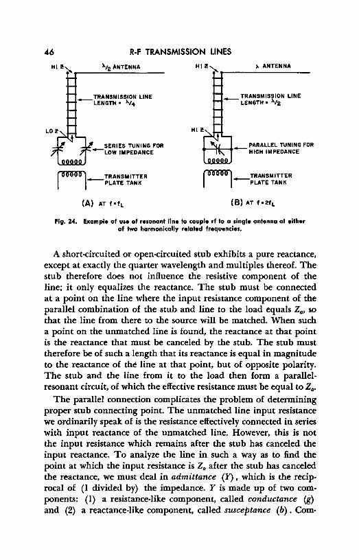
46 R-F TRANSMISSION LINES
>-12ANTENNA
TRANSMISSION LINE - lENGTH • >-14
SERIES TUNING FOR -LOW IMPEDANCE
~-TRANSMITTER I I PLATE TANK
(A) AT f•fL
>, ANTENNA
_ TRANSMISSION LINE LENGTH• >-12
~-TRANSMITTER I I PLATE TANK
(B) AT f•2fL
Fig. 24. Example of use af resonant line to couple rf to a single antenna at either of two harmonically related frequencies.
A short-circuited or open-circuited stub exhibits a pure reactance, except at exactly the quarter wavelength and multiples thereof. The stub therefore does not influence the resistive component of the line; it only equalizes the reactance. The stub must be connected at a point on the line where the input resistance component of the parallel combination of the stub and line to the load equals Z,,, so that the line from there to the source will be matched. When such a point on the unmatched line is found, the reactance at that point is the reactance that must be canceled by the stub. The stub must therefore be of such a length that its reactance is equal in magnitude to the reactance of the line at that point, but of opposite polarity. The stub and the line from it to the load then form a parallelresonant circuit, of which the effective resistance must be equal to Z0 •
The parallel connection complicates the problem of determining proper stub connecting point. The unmatched line input resistance we ordinarily speak of is the resistance effectively connected in series with input reactance of the unmatched line. However, this is not the input resistance which remains after the stub has canceled the input reactance. To analyze the line in such a way as to find the point at which the input resistance is Z0 after the stub has canceled the reactance, we must deal in admittance (Y) , which is the reciprocal of (1 divided by) the impedance. Y is made up of two components: (1) a resistance-like component, called conductance (g) and (2) a reactance-like component, called susceptance (b). Com-

APPLICATIONS OF TRANSMISSION LINES
MATCHED
LOAD
"~
Fig. 25. How a stub may be conneded to a line to provide matching.
47
ponents g and b combine to form Y in the same way that R and X combine to form Z. The stub is chosen so that the b of the stub is equal and opposite in polarity to the b of the line. Then the conductance remaining is the true total conductance, and its reciprocal is the resistance component, which must be equal to Z0 at the stub connecting point.
The variations of conductance, g, and susceptance, b, for a typical case of a line with a SWR of 2 are shown in Fig. 26. These variables are expressed in relation to g0, the conductance represented by Z0 •
The stub connecting point is chosen at the place where line g = g0 •
By following the vertical line down to the b curve, we see that b at that point is approximately 0. 72 g0 • Since b is negative (inductive) , a stub with a positive b (capacitive) must be used. The length of the stub can be determined by the formulas for z, given earlier, remembering that b = - I /x. In this case, an open-ended stub should be about 0.1,\ long and is connected to point 0, and a shorted stub should be about 0.15,\ long and connected to point S.
Notice in Figs. 26 and 27 that there are two possible stub connecting points near each voltage maximum. The connecting point nearer the load is always best matched by an open-ended stub (because for the same g it is much shorter than a shorted stub). The connecting point nearer the source from the voltage maximum is always best matched by a shorted stub. If the SWR of the line is measured, and the locations of the voltage maxima (or minima) are noted, the stub location can be determined with reference to the voltage maximum nearest to the load, without knowledge of the characteristics of the load. (See Fig. 27.)
The calculation of stub locations and lengths is a rather complex process, and the foregoing description has been included to explain
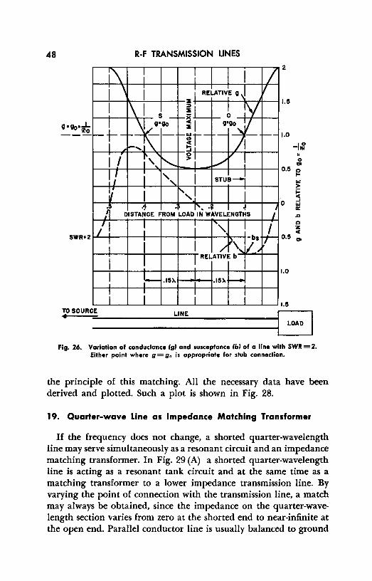
48
G•Qo•.L i!o ---
R-F TRANSMISSION LINES
1.0
-I~ " 0
"' 0.5 ~
l&I > 5
--------------,---+---~o ~ II:
.Cl
0 z C
0.5 .,.
.15ll.t-----l.15ll.
._____._ _ _.__..____. _ _.__..____. _ _.__..____. _ _. 1.5 TO SOURCE LINE ,..
1
__ __,
-------------------1 LOAD
Fig. 26. Variation of conductance Cg) and susceptance Cb) of a line with SWII = 2. Either point where g = 9• is appropriate for stub connection.
the principle of this matching. All the necessary data have been derived and plotted. Such a plot is shown in Fig. 28.
19. Quarter-wave Line as Impedance Matching Transformer
If the frequency does not change, a shorted quarter-wavelength line may serve simultaneously as a resonant circuit and an impedance matching transformer. In Fig. 29 (A) a shorted quarter-wavelength line is acting as a resonant tank circuit and at the same time as a matching transformer to a lower impedance transmission line. By varying the point of connection with the transmission line, a match may always be obtained, since the impedance on the quarter-wavelength section varies from zero at the shorted end to near-infinite at the open end. Parallel conductor line is usually balanced to ground
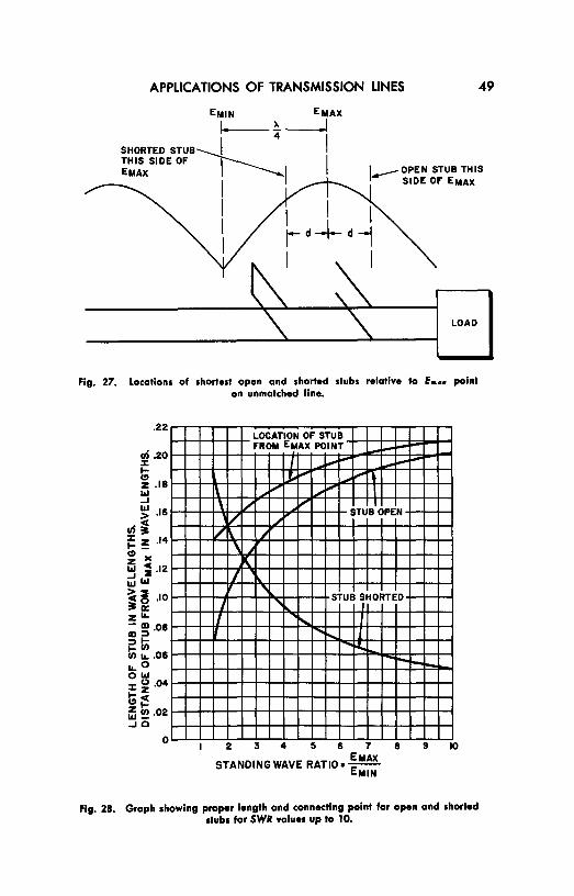
APPLICATIONS OF TRANSMISSION LINES 49
EMAX
i----~-----l SHORTED STUBr----'
4
I THIS SIDE OF I EMAX I
.-----. I , ___ OPEN STUB THIS
SIDE OF EMAX
I I I
LOAD
Fig. 27. Locations of shortest open ond shorted stubs relative to E... point on unmotched line •
. 22
in .20 ::c t; z .18 l&I .J
~ .16
cri ; ~ ~ .14 c:> )( z C l&I 2 .12 ii:l w
~~ .10 31= 0: zi.. ;;; ~ .08
~I;; 11> 1&. .06 .._o 01&1 ::c () .04 I- z c:>~ ~ !!?-02 .J 0
0
LOCATION OF STUB FROM EMAX POINT ,_ ---I i..-- 1- i--
t- - i..,,, l \ ~" ~"'" I \ 1 ..... V I
'I/ ,," STUB OPEN
I.I~ ~
' ~ I(
! J , ... ~
' .... STUB SHORTED
I ~ ""i....
'"~ - .... 1-- ......
2 34 56 7 8 9 10
STANDING WAVE RATIO• EEMAX MIN
Fig. 28. Graph showing proper length and connecting point for open and shorted stubs for SWII volues up to 10.
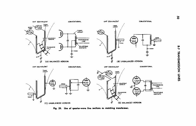
--,)\
UHF EQUIVALENT
// /
I I
I I
, , f
/-AOJUSTAIU / CONTACTS I I I
CONVENTIONAL
J:
TRANSMISSION LINE
'ADJUSTABLE CONTACTS
I ?' (A) BALANCED VERSION
UHF EQUIVALENT
TUNED CIRCUIT
CONVENTIONAL
. '\\
q (C) UNBALANCED VERSION
........... ,
>\
UHF EQUIVALENT
TUNED I
CIRCUIT //
/ I
f
I I
:
CONVENTIONAL
/
. \
'\
l I ?' (B) UNBALANCED VERSION
UHF EQUIVALENT CONVENTIONAL
q (0) BALANCED VERSION
Fig. 29. Use of quarter-wove line sectloM 01 motchlng transfonter.
TRANSMISSION LINE
'ADJUSTABLE. CONTACTS
u, 0
:,a .;.. -I
~ z en 3'; c;; en 0 z C: z C:

APPLICATIONS OF TRANSMISSION LINES 51
r " 2
L HIGH~/
~o---.....
-ANTENNA
7 " 4
J MATCHING
TRANSFORMER
(A) J ANTENNA
ANTENNAS
" 2 a b
½ '
-t TRANSFORMER
( 8) HALF-WAVE ANTENNAS IN PHASE
Fig. 30. Use of quarter-wave transformer with antennas.
and thus requires a balanced matching device; hence both sides of the line are connected to the same impedance point on either conductor. Coaxial cable is usually unbalanced, with its outer conductor grounded. Figure 29 (B) shows an unbalanced impedance transformer. In both examples, the line segment is used as a step-down transformer from the high impedance plate of an amplifier or oscillator to a lower impedance transmission line.
In a receiver, a problem arises where the grid of the first tube has a high impedance. It is necessary to employ a similar arrangement, in which the low impedance line is matched to the high impedance grid. In Fig. 29, C and D show graphically how balanced and unbalanced transmission line segments may be employed to perform this duty. The same principle may be used in matching antennas, as illustrated in Fig. 30. At A is the popular "J" antenna, which is simply a half-wave whose high-impedance end runs right into a quarter wave whose other end is shorted and grounded. The transmission line is then moved down the quarter-wave section until its impedance is matched. At (B) is the connection for two half-wave antennas in phase. Again, the high-impedance ends of the antennas connect to the top of the quarter-wave transformer and the line is

52 R-F TRANSMISSION LINES
"tapped down" on it. In this case the transformer also keeps voltage at point a 180 degrees out of phase with voltage at point b, so that the antennas operate in phase.
20. Lecher Wire Line
Often the operational frequency of a transmitter must be measured. A popular device for this purpose is a Lecher wire frequency meter. The principle of operation directly follows the previously discussed theory; by creating standing waves on a transmission line segment (usually greater than a half wavelength) and measuring the linear distance between maximum or minimum points of current (or voltage) , we may determine the wavelength of operation, and consequently the frequency.
R-f energy is usually coupled into the system by use of an inductive loop (Fig. 31A), one end of which is connected to the Lecher wires, with the other end within inductive proximity of the oscillator tank coil. Energy induced in this manner flows down the Lecher wires to a shorting bar whose position along the line is adjustable. At this point reflection takes place and energy bounces back to the tank circuit. What the tank circuit sees when looking into the Lecher wires depends upon the position of the shorting bar. If the shorting bar is located a half wavelength from the tank, a short circuit is seen; if it is located at odd multiples of a quarter wavelength, an open circuit is seen. At points where the tank sees a short circuit, most of its energy will be absorbed by the Lecher wires.
Of course, no energy is absorbed when the tank sees an open circuit. To sense the change of energy in the tank circuit at different positions of the shorting bar, a light bulb is also inductively coupled to the tank circuit. Except when the tank sees a short circuit in the Lecher wires, its energy is sufficient to light the bulb.
Operation is very simple. The light bulb is first made to light by placing it close enough to the tank, and the shorting bar is moved to either end of the Lecher wire system. As the shorting bar is gradually moved to the other end, a point of series resonance (multiple of half wavelength distance from tank) is reached. This point (where the light dies out) is carefully marked. The shorting bar is now moved in the same direction until the next point is reached where the bulb is extinguished. The distance between these two points is a half wavelength. From this measurement the frequency may be determined from:

APPLICATIONS OF TRANSMISSION LINES
OOBUL.B
:]] /
MOVABL.E ~!~K SHORTING COIL. BAR
E '""~'--L.OOPS 2
SHORTED
END\
___...\~ TRANSMISSION~ BUL.B L.INE SEGMENT TANK Cl RCUIT OF OSC
(A)
Fig. 31. Lecher wire frequency meter.
. 5905 Frequency m megacycles = d. b • • • h 1stance etween pomts m me es
53
Instead of a bulb, the plate current of the oscillator, indicated by a meter, may be observed. At half-wave intervals, the plate current rises sharply.
Because of the size, this device is of little use below 100 megacycles. For example, at broadcast frequencies it would be hundreds of feet long.
21. Supporting Stubs
If the frequency is increased to 1000 me and over, the dielectric losses of ordinary transmission line are prohibitively high. A rigid

54 R-F TRANSMISSION LINES
SHORTED QUARTERWAVELENGTH SUP· PORTING STUBS
SUPPORTING QUARTER WAVELENGTH STUB
GROUND
CLOSED END
PARALLEL CONDUCTOR TRANSMISSION LINE
(A)
COAXIAL CABLE
( B)
Fig. 32. Use of quarter-wave stubs as physical supports for line.
quarter wavelength transmission line stub is often used as a support at these frequencies.
Figure 32 (A) shows just such an arrangement for parallel conductor line. Note that the shorting bar is grounded and that the open end is connected to the transmission line. Now any r-f energy in the line that attempts to enter the stub will find an extremely high impedance at the input of the stub. The impedance would be resistive, because the stub is actually a parallel resonant circuit. An additional advantage of the quarter-wavelength supporting stub is that it provides a low resistance path for de to fl.ow to ground.
As an example, suppose a line is carrying energy at 400 me and has a velocity constant of 0.9. The length of a quarter-wave stub can be obtained as follows:
984 984 . A./4 = ¼ x-,-X VC = ¼ X 400 X 0.9 = 0.55 ft.= 6% mch
As the frequency is increased, stubs are used almost exclusively as the insulating and supporting medium. Figure 32 (B) illustrates the coaxial version of this stub. The disadvantage of the system is that the stubs are effective insulators at only one frequency. By proper Q-lowering design of stubs, a limited frequency deviation is permissible.
Since, when measuring the SWR, we must not disturb the conditions already existing on the line, it is usually easier to use a high resistance voltmeter for the purpose. Figure 33 shows a high resistance r-f voltmeter being used. It consists of a quarter-wavelength transmission line segment with an r-f ammeter connected to one
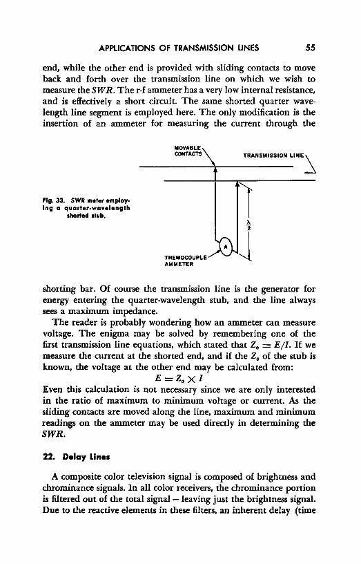
APPLICATIONS OF TRANSMISSION LINES 55
end, while the other end is provided with sliding contacts to move back and forth over the transmission line on which we wish to measure the SWR. The r-f ammeter has a very low internal resistance, and is effectively a short circuit. The same shorted quarter wavelength line segment is employed here. The only modification is the insertion of an ammeter for measuring the current through the
Fig. 33. SWR meter employ-1 n g a quarter-wavelength
shorted stub.
MOVABLE CONTACTS
THEMOCOUPLE AMMETER
TRANSMISSION LINEi
shorting bar. Of course the transmission line is the generator for energy entering the quarter-wavelength stub, and the line always sees a maximum impedance.
The reader is probably wondering how an ammeter can measure voltage. The enigma may be solved by remembering one of the first transmission line equations, which stated that Z0 = E/1. If we measure the current at the shorted end, and if the Z0 of the stub is known, the voltage at the other end may be calculated from:
E =Z0 XI Even this calculation is not necessary since we are only interested in the ratio of maximum to minimum voltage or current. As the sliding contacts are moved along the line, maximum and minimum readings on the ammeter may be used directly in determining the SWR.
22. Delay Lines
A composite color television signal is composed of brightness and chrominance signals. In all color receivers, the chrominance portion is filtered out of the total signal - leaving just the brightness signal. Due to the reactive elements in these filters, an inherent delay (time

56 R-F TRANSMISSION LINES
lag) is introduced, which causes the chrominance signals to lag the brightness signal in some receivers by about 1.2 microseconds.
To eliminate color misregistration, it is essential that something be done to the brightness signal so that it does not reach the picture tube before the lagging chrominance signals. The time delay of the brightness signal is accomplished by using a delay line.
There are two major varieties of delay lines: the distributed constant line and the lumped constant line. (The latter is often called an "artificial transmission line.") The principle of operation of a distributed constant delay line follows closely the previous development of transmission line theory. In fact, the only theoretical difference between the two is the amount of inductance and capacitance per unit length.
The velocity of an electromagnetic wave in a transmission line
at radio frequencies is given by ~- From this relationship it
can be seen that an increase of L and C of a transmission line will lower the velocity of any wave travelling through the line. As the velocity decreases, so does the wavelength; hence a lower velocity will mean a greater number of wavelengths for a given physical distance of transmission line. Since the wave's lagging phase angle with respect to the source increase~ at the rate of 271' radians (360°) for each wavelength covered, the total phase angle of displacement for a given distance from the source will be greater if the velocity decreases.
Physically, a distributed constant delay line is slightly different from ordinary coaxial cable. (See Fig. 34.) The delay line consists of a center helical or spiral wire conductor wound around a circular insulating form. Over this wire is a layer of insulation. The next layer is a braided conducting shield that is grounded, and surrounding the entire cable is a protecting and insulating plastic sheath.
Any transmission line could be used for a delay line, but since the propagation velocity on most lines is well over 50 percent of the speed of light, a delay of 0.5 microsecond would necessitate a line more than 500 feet long. Some commercial delay lines decrease the wave velocity to such an extent that a delay time of up to 0.5 microsecond is possible in one foot of length.
Many delay lines have a characteristic impedance ranging around 1000 ohms. All the rules about terminating the line in its Z0 must be followed. Reflections will cause a distortion (of the wave) that is dependent on frequency.
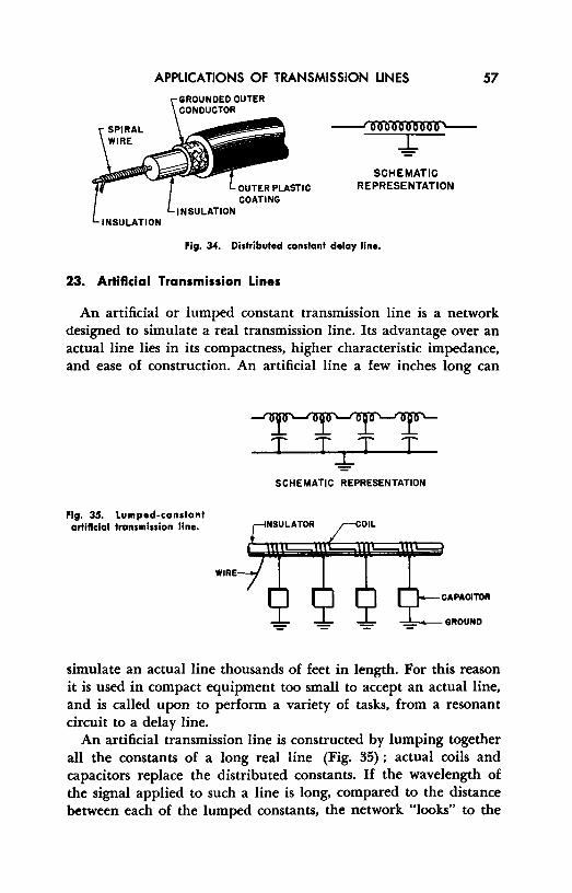
APPLICATIONS OF TRANSMISSION LINES
OUTER PLASTIC COATING
INSULATION
SCHEMATIC REPRESENTATION
Fig. :U. Distributed constant delay line.
23. Artificial Transmission Lines
57
An artificial or lumped constant transmission line is a network designed to simulate a real transmission line. Its advantage over an actual line lies in its compactness, higher characteristic impedance, and ease of construction. An artificial line a few inches long can
Fig. 35. Lumped-constant artiflcial transmission line.
T T-f:T T SCHEMATIC REPRESENTATION
simulate an actual line thousands of feet in length. For this reason it is used in compact equipment too small to accept an actual line, and is called upon to perform a variety of tasks, from a resonant circuit to a delay line.
An artificial transmission line is constructed by lumping together all the constants of a long real line (Fig. 35) ; actual coils and capacitors replace the distributed constants. If the wavelength of the signal applied to such a line is long, compared to the distance between each of the lumped constants, the network "looks" to the

58 R-F TRANSMISSION LINES
travelling wave as an actual transmission line. The upper frequency limit at which the line ceases to look "real" is called the critical frequency.
24. Transmission Line Oscillator Tank
At low frequencies, coils and capacitors are relatively efficient, while a quarter wavelength line segment is large and unwieldy. 'As the frequency is increased above 300 or 400 megacycles, the amount of inductance and capacitance needed is so small and the losses in coils and capacitors become so great that they are of little use. Now the size of a quarter-wavelength line section becomes con~ veniently small enough so that it may be used for every one of the applications discussed in this chapter.
Perhaps the most common use of a quarter-wavelength line is to act as a resonant circuit, such as might be used as an oscillator tank circuit. Let us again consider what happened at the input terminals of the shorted quarter wave line in Fig. 36 (A) . The generator sees a maximum impedance which is purely resistive at one frequency. If the frequency is raised, the impedance drops rapidly and is capacitative; if the frequency is lowered, the impedance drops and is inductive. The line has zero impedance for direct current. The description above fits exactly a parallel resonant circuit. If, on the other hand, the line is open-circuited (Fig. 36B) , the generator sees a minimum impedance only at the resonant frequency. The impedance rises on either side of resonance - inductive above and capacitive below - and will not pass de. An open-circuited quarterwavelength line thus looks like a series resonant circuit. An example of how a transmission line can be used as a tuned circuit in a simple uh£ oscillator is given in Fig. 37.
25. Transmission Lines in UHF and Microwave Region
The problems confronting conventional transmission line operation in the high uh£, or sh£ (above 3000 me) region become enormous. Radiation, dielectric, and conductor losses, in many cases, consume most of the power intended to be propagated down the line.
Although the losses in both parallel conductor line and coaxial line increase with frequency, they do not increase at the same rate. Due to high radiation losses, parallel conductor line is not usually

APPLICATIONS OF TRANSMISSION LINES 59
0=~ 1-~-1 ~
~ _£7 1-~-J -~
4 4 (A)
Fig. 36. Quarter-wavelength line as resonant circuit.
-
-
e+
ULTRAUDION OSCILLATOR (LOW FREQ.)
(A)
RFC B+
ULTRAUDION OSCILLATOR
(UHF)
(B)
Fig. 37. Use of transmission line section as tuned circuit in a uhf oscillator.
(B)
used much above l 000 me. Coax, as previously explained, is not susceptible to radiation loss at any frequency, when properly used.
The stipulation was made for parallel wire line that radiation would be low only when the separation between conductors was less than 0.01 wavelength at the frequency of operation. To maintain a conductor spacing of less than this amount, and at the same time increase the frequency (decreasing the wavelength), the conductor spacing must be reduced. There is, however, a lower limit on the distance, governed (if not by constructional difficulties) by the
. E2 amount of power (P) transmitted on the line. Smee P = Z' and
0
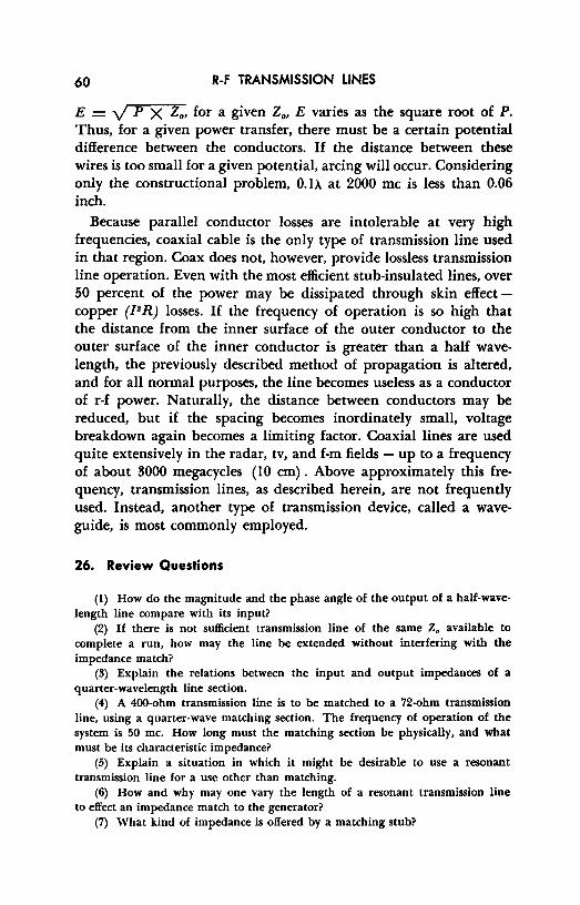
60 R-F TRANSMISSION LINES
E = y P X Z0 , for a given Z0, E varies as the square root of P. Thus, for a given power transfer, there must be a certain potential difference between the conductors. If the distance between these wires is too small for a given potential, arcing will occur. Considering only the constructional problem, 0.1..\. at 2000 me is less than 0.06 inch.
Because parallel conductor losses are intolerable at very high frequencies, coaxial cable is the only type of transmission line used in that region. Coax does not, however, provide lossless transmission line operation. Even with the most efficient stub-insulated lines, over 50 percent of the power may be dissipated through skin effect -copper (l'R) losses. If the frequency of operation is so high that the distance from the inner surface of the outer conductor to the outer surface of the inner conductor is greater than a half wavelength, the previously described method of propagation is altered, and for all normal purposes, the line becomes useless as a conductor of r-f power. Naturally, the distance between conductors may be reduced, but if the spacing becomes inordinately small, voltage breakdown again becomes a limiting factor. Coaxial lines are used quite extensively in the radar, tv, and £-m fields - up to a frequency of about 3000 megacycles (IO cm). Above approximately this frequency, transmission lines, as described herein, are not frequently used. Instead, another type of transmission device, called a waveguide, is most commonly employed.
26. Review Questions
(l) How do the magnitude and the phase angle of the output of a half-wavelength line compare with its input?
(2) If there is not sufficient transmission line of the same z. available to complete a run, how may the line be extended without interfering with the impedance match?
(3) Explain the relations between the input and output impedances of a quarter-wavelength line section.
(4) A 400-ohm transmission line is to be matched to a 72-ohm transmission line, using a quarter-wave matching section. The frequency of operation of the system is 50 me. How long must the matching section be physically, and what must be its characteristic impedance?
(5) Explain a situation in which it might be desirable to use a resonant transmission line for a use other than matching.
(6) How and why may one vary the length of a resonant transmission line to effect an impedance match to the generator?
(7) What kind of impedance is offered by a matching stub?
APPLICATIONS OF TRANSMISSION LINES
(8) What is the function of a matching stub in terms of its impedance? (9) Explain how and why stub matching is possible.
61
(10) If a quarter-wavelength impedance matching transformer such as that illustrated in Fig. 29-B is adjusted to correctly match the output of a transmitter to its transmission line, what will be the quantitative effect on the input and output connections of this transformer with a decrease in frequency?
(II) When is it practical to use a shorted quarter-wavelength transmission line as a resonant circuit? Why?
(12) If a Lecher wire frequency meter is used to measure an unknown frequency from a transmitter, and it is noted that a dip in the indicating bulb's brightness occurs at two points when the shorting bar is moved from one end of the Lecher wire system to the other, what is the frequency of operation if the distance between these two points is 3.2 feet?
(l!l) Why are Lecher wire frequency meters not used extensively below about 100 me?
(14) What is the main disadvantage of transmission line stub insulators? (15) How can a low-resistance r-f ammeter be used to measure transmission
line voltage without disturbing the line? (16) Why are delay lines necessary in color tv receivers? (17) How do the total inductance and total capacitance of a delay line affect
its time delay? (18) How does the length of a delay line affect its delay?
INDEX
Admittance, 15, 46 Artificial trans111ission lines, 56, 57, 58
Characteristic impedance, 13, 15, 16, 17, 20, 21, 23
Coaxial cable, 1, 2, 37, 51, 58, 59, 60 Conductance, 15, 46 Copper loss, 25, 37 Critical frequency, 58
Delay lines, 55, 56 Dielectric leakage, 37 Distributed constant line, 56
Half-wavelength line, 26, 39, 40, 41 Hollow dielectric parallel conductor, 4
Impedance curve, 26 1.mpedance match, 17 Impedance mismatch, 21 Impedance per unit length, 5 Impedance value, open circuit load, 27, 28 Impedance value, short circuit load, 27, 28 Incident wave, 20, 21, 22, 24 Induction loss, 37 Input impedance, 32, 33
"J" antenna, 51
Lecher wire line, 52 Line losses, 33, 36, 37 Line matching with stubs, 45, 46, 47 Line termination, 17, 22 Loop, 24 Lumped constants distributed, 4, 5
Lumped inductance, 5
Maximum power transfer, 23
Node, 24
Open wire, 3
Parallel conductor transmission line, 3, 24, 36, 37, 51, 58, 59, 60
63
Parallel wire line, 4 Phase shift, 12, 13 Physical length of line, formula for, 10 Pipe-type coax, 3 Polyethylene, 3
Quarter-wavelength line, 26, 33, 42, 43, 44, 48, 51
Radiation loss, 36 Reflected wave, 20, 21, 22, 23, 24, 26 Reflections, 17, 18, 19, 20, 21 Reflection coefficient, 22 Resonant lines, 32, 33, 44, 45
Shielded two-conductor transmission line, 4 Shunt capacitance, 5
Shunt dielectric leakage, 5, 8, 37 Skin effect, 7, 8 Solid dielectric type, 2, 3 Supporting stubs, 53, 54, 55 Susceptance, 15, 46 Standing wave ratio, 28, 29, 30, 31, 32,
36, 55 Standing waves, 23, 24, 25, 26, 27 Stubs, 3
Transmission line oscillator tank, 58 Transmission lines, introduction, 1 Transmission lines, uhf, microwave region,
58, 59, 60 Tuned line, 32 Twinax, 3, 4 Twin lead, 3 Twisted lead, 4, 5 Types of lines, 2, 4
Variations of constants, 5, 7, 8
Wavelength and velocity, 9, 10, 11, 12 Wire resistance, 5, 6
"Zepp" antenna, 45