REGRESSION PLANES TO IMPROVE THE PYTHAGOREAN

PERCENTAGE

A regression model using common baseball statistics to project offensive and defensive efficiency

by

Dennis Moy

A thesis submitted in fulfillment of the requirements for the degree of honors in

Statistics

University of California - Berkeley

2006

UNIVERSITY OF CALIFORNIA - BERKELEY

ABSTRACT

Prediction Planes for the Pythagorean Percentage

by Dennis Moy

Advisor: Professor David Aldous Department of Statistics

In 1985, Bill James, arguably the most renowned analytical baseball statistician, devised

a very simple, but effective formula that predicted a team’s winning percentage given

its runs scored and runs allowed. Despite its remarkable accuracy, this model, coined

Pythagorean expectation, was used primarily on seasons of the past rather than

performance forecasts. This thesis develops prediction models for runs scored and

runs allowed that will be converted by Pythagorean expectation to winning

percentages. Data from the past twenty years were taken from four different sources

of baseball statistics via the internet to produce 562 arrays that underwent

computations through GRETL to create two different ordinary least-squares

regression planes (offense and defense). The GRETL outputs yielded robust models

that had strong positive R2 results with significant F-statistics from the Wald test that

evaluated the planes’ goodness of fit, which with a potentially adjusted Pythagorean

expectation, can now forecast future winning percentages. Armed with this knowledge

and a little calculus, baseball executives can determine which talent is more valuable

when building a successful team to maximize winning percentage.

i

TABLE OF CONTENTS

List of Figures and Tables...................................................................................................... ii Acknowledgements................................................................................................................ iii Glossary................................................................................................................................... iv Introduction and Background ............................................................................................... 1 Materials and Method............................................................................................................. 8 Data Analysis and Findings.................................................................................................. 10 Discussion of Results............................................................................................................ 20 Conclusion and Extensions ................................................................................................. 25 Appendix (Derivations)........................................................................................................ 28 Bibliography........................................................................................................................... 31

ii

LIST OF FIGURES AND TABLES

Number Page Table 1: Summary Statistics from GRETL........................................................................ 10

Figure 1: Scatterplot of Runs (Adjusted) versus Year....................................................... 11

Figure 2: Scatterplot of OBP versus Year .......................................................................... 13

Figure 3: Scatterplot of SLG versus Year........................................................................... 13

Figure 4: Scatterplot of WHIP versus Year ....................................................................... 14

Figure 5: Scatterplot of DER versus Year.......................................................................... 14

Table 2: OLS Estimates of Runs Scored (Adjusted) versus OBP and SLG .................. 15

Figure 6: Fitted, Actual Plot of Runs Scored (Adjusted) versus OBP and SLG......... 16

Figure 7: Residuals for Runs Scored (Adjusted) Regression Model ............................. 17

Table 3: OLS Estimates of Runs Allowed (Adjusted) versus WHIP and DER............ 17

Figure 8: Fitted, Actual Plot of Runs Allowed (Adjusted) versus WHIP and DER..... 18

Figure 9: Residuals for Run Allowed (Adjusted) Regression Model............................... 19

iii

ACKNOWLEDGMENTS

I would like to express my sincere appreciation to my parents first and foremost for

sending me through school for the past 19 years and always making sure I was aiming

high and giving my best efforts. Also, I want to thank Professor David Aldous for

being a helpful advisor who allowed me to apply all that I have learned to a topic I

love. Thanks to the immortal Team Savage, who provided a gateway each week for me

to chase and realize the dream of an intramural softball championship. Also, I need to

thank my two roommates, Kevin and Herman, for dealing with my complaints about

doing this for a whole semester and the rest of my friends, for using my thesis as an

excuse for not going out and enjoying my last semester in college. Thank you to Mr.

Spellicy for being a great mentor and telling me to pursue what I enjoy. Most

importantly, I need to thank Ms. Delfino for suggesting me to take Advanced

Placement Statistics as a sophomore at Lowell High School, as that paved the road for

my interest and major in statistics. And last but not least, I want to state my deep

gratitude to Eva for keeping me on top of my thesis and helping me edit until the

perfect version came into fruition.

iv

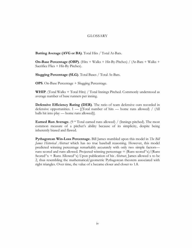
GLOSSARY

Batting Average (AVG or BA). Total Hits / Total At-Bats.

On-Base Percentage (OBP). (Hits + Walks + Hit-By-Pitches) / (At-Bats + Walks + Sacrifice Flies + Hit-By Pitches).

Slugging Percentage (SLG). Total Bases / Total At-Bats.

OPS. On-Base Percentage + Slugging Percentage.

WHIP. (Total Walks + Total Hits) / Total Innings Pitched. Commonly understood as average number of base runners per inning.

Defensive Efficiency Rating (DER). The ratio of team defensive outs recorded in defensive opportunities. 1 — [(Total number of hits — home runs allowed) / (All balls hit into play — home runs allowed)].

Earned Run Average. (9 * Total earned runs allowed) / (Innings pitched). The most common measure of a pitcher’s ability because of its simplicity, despite being inherently biased and flawed.

Pythagorean Win-Loss Percentage. Bill James stumbled upon this model in The Bill James Historical Abstract which has no true baseball reasoning. However, this model predicted winning percentage remarkably accurately with only two simple factors—runs scored and runs allowed. Projected winning percentage = (Runs scored^x)/(Runs Scored^x + Runs Allowed^x) Upon publication of his Abstract, James allowed x to be 2, thus resembling the mathematical/geometric Pythagorean theorem associated with right triangles. Over time, the value of x became closer and closer to 1.8.

- 1 -

§ Introduction and Background

Open up the newspaper. Which sections use numbers or quantifiable data to transmit their

news? Sure, the business section has a plethora of figures for trade activity in stocks, bonds and other

markets. People interpret these numbers to gauge the value of their holdings and their holdings’

competition. A reader can quickly see if Google outperformed Yahoo during the previous day’s

trading. But where else in the newspaper do you see numbers? Flip to the sports page. The March 22,

2006 version of a San Francisco newspaper has these results scattered among its sports section:

San Antonio Spurs 107, Golden State Warriors 96 San Jose Sharks 6, St. Louis Blues 0 Japan 10, Cuba 6 Oakland Athletics 6, San Francisco 4

However, along with these straightforward scores, there are boxscores that tell the story of

each game. Similar to the business section, these numbers in the boxscores gauge the value of each

player that participated in the game and his or her teammates and opponents. A reader can quickly

look up whether Tim Duncan performed better than Jason Richardson and get a good idea of how the

Oakland Athletics mustered enough runs to defeat their cross-town rivals, the San Francisco Giants, in

a spring training exhibition game. Every major American sports game played has a resulting boxscore,

but baseball is different among the four major sports—football, basketball, and hockey. Its regular

season of 162 games is significantly longer than other sports’—hockey and basketball both have 82

games while football has only 16. During their seasons, football players play once a week on the

gridiron; hockey players rarely skate on back-to-back days for games on the rink; basketball players

barely spend the majority of a week in front of a crowd on a court; however, baseball players

frequently play every day or night for two straight weeks, sometimes even twice a day. With all of this

action, it is fast and easy for every baseball player to build up statistics with significant repetition (or

- 2 -

sample size). The best position players on each team easily accumulate 500 at-bats, the healthiest

starting pitchers face at least 800 batters, and the best relief pitchers enter the game 60 or more times

during the regular season. Above the other three major sports, baseball stands out as the most

quantifiable and most statistically developed; incidentally, this started before computers were

commonplace in every home and office.

The origins of baseball have been widely disputed; the most common myth credits a Civil War

general, Abner Doubleday, with the “invention” of baseball in 1839 even though there has been

documented proof that versions of the game existed prior to 1839. In 1845 though, Alexander

Cartwright published the first formal rulebook for the game of baseball; the first resemblance of a

boxscore, or “abstract” as it was called then, appeared in the October 22, 1845, New York Morning News

issue. Soon after, Henry Chadwick devised the most primitive statistics—batting average and earned

run average—to valuate different players on different teams. However, it would take the greater part

of a century before baseball statistics reached a new echelon. As the game grew more popular, stat-

filled books such as Who’s Who in Baseball and Balldom: The Britannica of Baseball were published in the

1910s by trailblazing statisticians. During this time, the value of a player was judged by the eyes of old,

leather-skinned scouts who would spend many summer days under the sun scouring local baseball

games to discover talent; a player’s past statistics merely served as tools for banter among the crowds

of fans. Signs of progressive change surfaced in the late 1940s for the world of baseball and the world

of baseball statistics as well. Branch Rickey, one of the most innovative men among the ranks of a

baseball team’s front ranks, spearheaded what seemed to be a radical baseball evolution. After

developing the first full-time spring training facilities which are a staple of March in Arizona and

Florida today, Branch Rickey shook Major League Baseball upside down when he signed Jackie

Robinson in 1947 to the Brooklyn Dodgers to break the color barrier. Below the hoopla of this

- 3 -

transaction, Rickey welcomed a Canadian, Allan Roth, to his team hours before the Robinson signing.

No, Allen Roth was not the first Canadian baseball player, but Roth was a statistician who had ground-

breaking theories on a new statistic to evaluate offensive performance. Batting average conspicuously

omits bases on balls in its computation; however, Allan Roth compensated for this omission when he

helped Rickey introduce the new statistic of on-base percentage or OBP. Logically, a walk was as good

as a base hit, since the batter did not cause an out and reached base safely after judging four balls

outside of the strike zone or being struck by a pitched ball; batting average fails to acknowledge this

skillful performance as on-base percentage does, but it would take until the 1960s for more abstract

analysis of baseball statistics.

Two publications during this decade invigorated younger, mathematical minds to pursue the

unexplored realm of statistics in baseball. Earnshaw Cook penned a theory-intensive book titled

Percentage Baseball which nebulously disproved the effects of many common, traditional baseball

strategies such as stealing bases and using sacrificing bunts. This book was written too early for its

time, but it did pave the way for researchers across the nation to collaborate for a tour de force that

was published in 1969. The Baseball Encyclopedia, a bestseller published by Macmillan, was the collective

product of many man-hours of perusing old boxscores to build a source of reference on every baseball

player and how he performed during his career. Not only did this book introduce the use of

technology to compute new baseball statistics, but it brought together a legion of baseball statisticians

for the first ever meeting of the Society for American Baseball Research.

The Society for American Baseball Research, or SABR for short, was born in 1971 when 16

mean gathered in Cooperstown to discuss the importance of preserving baseball history; membership

swelled to 6,000 members in 15 years and over time, baseball statisticians became known as

- 4 -

sabermetricians because of this organized group. Ironically, the man who would contribute most to

sabermetrics after the society’s inception could not afford the $25 cost of The Baseball Encyclopedia.

In 1977, Bill James finished his masterpiece, The Bill James Historical Baseball Abstract, which

brought baseball research to a new level. Unlike books in the past, James wrote about topics that were

never thought about; for instance, he went out of the proverbial box and hypothesized how to valuate

a player by the number of runs he contributed to the team. Aside from merely reporting mundane

statistics like batting average or on-base percentage, this book identified that runs were the key

ingredient in allowing a team win. Runs were the most valued asset in baseball—score more, and your

team has a better chance of winning; prevent your opponent from scoring, and once again your team

has a better chance of winning. Branching out even farther, James essentially stumbled upon a key

model that estimated a team’s winning percentage using runs scored and runs allowed that mystically

resembled the Pythagorean theorem in the mathematical and geometric world that related the sides of

a right triangle. The model was precise enough that teams began to use it to assist them in evaluating

which players to add or subtract to their team in order to judge the transaction’s effect on winning

percentage. He appropriately coined the model as the Pythagorean Win-Loss Percentage. The glory of

this model was that the two inputs—runs scored and runs allowed—created a projected winning

percentage which was independent of which league the team played in, the length of the season, and

most importantly, during what era the team played. Initially, James used this formula to attribute

whether teams were lucky or unlucky in seasons past; because of the abovementioned independences,

deviation from the estimated winning percentages were simply blamed on good or bad luck.

Following James’ footsteps by tinkering with the exponent in the model, many sabermetricians

used historical statistics for every team in every season to minimize the residuals to create the best

fitting Pythagorean Win-Loss Percentage model (with an exponent that floated around 1.8). But these

- 5 -

sabermetricians seemingly never used this model to forecast future winning percentages, for there were

only primitive (and complex) models that estimated runs scored and runs allowed. Bill James’ “runs

created” was such a model that used eleven input variables, which aside from being too difficult to

compute (as it needed the values for hits, walks, times caught stealing, times hit by a pitch, double

plays, total bases, stolen bases, intentional walks, sacrifice bunts, sacrifice flies, and at bats), they

artificially inflated the correlation coefficients, thus deceptively implying importance. Also, there was

very little research into creating a model for runs allowed; despite the development of many non-

traditional pitching statistics, measuring a team’s fielding abilities was still unrealized. As computers

became more and more popular, baseball research began to accelerate.

By the 1990s, sabermetrics reached a new level of popularity with the advent of the internet

and the World Wide Web. A faction of the Society for American Baseball Research convened in 1994

with the mission of digitizing the boxscore of every single baseball game ever played. This group,

Retrosheet, Inc., is still at work today, trying to scour old newspapers for hardcopies of these

boxscores. As these records were digitized, they were made available via their website which gave birth

to a new breed of baseball “techies”. Sean Forman is one of these techies and he manipulated the

digitized boxscores to create baseball reference websites—dutifully titled Baseball-Reference.com and The

Baseball Archive—which had pages for every player and his statistics who played in the major leagues

and for every team as well. He even made his work free and accessible through spreadsheets and

retrievable through databases using Structured Query Language (SQL). Currently, Gary Cohen is

taking this research one step further by perusing for minor league statistics and posting them through

his website, TheBaseballCube.com. As these resources became so readily available, websites that require

membership such as BaseballProspectus.com performed very detailed analysis and consequently new

- 6 -

abbreviations for baseball statistics sprang up just as Franklin Roosevelt’s New Deal alphabet soup

deluged America during the Great Depression.

Ironically, it took a book not about baseball to put some of these abbreviations into the

mainstream. Michael Lewis, a well-known author because of his most prestigious bestseller Liar’s

Poker, finished Moneyball in 2003, which only used the context of baseball to emphasize the importance

of capitalizing on undervalued resources in a competitive market. In 2002, Lewis shadowed Billy

Beane, the general manager for the Oakland Athletics, to gain insight from the team’s front office.

Beane was a huge proponent of players with high on-base percentages, for his theory revolved around

the fact that a 9-inning game had a finite number of outs—27; on-base percentage was a measure of

player’s ability to avoid making an out by reaching base safely. Thus, by fielding a team full of players

who produced fewer outs on the average compared to other players, Beane theorized that the resulting

team would maximize offensive production. As a small-market team, the Oakland Athletics were

forced to dig deeper and investigate the subtle statistics of players, rather than the glowing statistics

such as batting average and home runs, since the large-market teams could spend more money and

sign these superstar players. Lewis’ book revolved around this concept and how the Oakland Athletics

were able to discover an undervalued resource and capitalize on its under-appreciation.

As The Bill James Historical Abstract became more popular in the baseball community, some

readers became skeptical of some James’ theories—one of which was Beane’s right-hand man, Paul

DePodesta, who Lewis relates about thusly on page 128 in Moneyball:

Baseball fans and announcers were just then getting around to the Jamesean obsession with on-base and slugging percentages. The game, slowly, was turning its attention to the new statistic, OPS (on-base plus slugging)…Crude as it was, it was a much better indicator than any other offensive statistic of the number of runs a team would score. Simply adding the two statistics together, however, implied they were of equal importance…An extra percentage point of on-base was as good as an extra percentage point of slugging.

- 7 -

Before his thought experiment Paul had felt uneasy with this crude assumption; now he saw that the assumption was absurd. An extra point of on-base percentage was clearly more valuable than an extra point of slugging percentage—but by how much? He proceeded to tinker with his own version of Bill James’s “Runs Created” formula. When he was finished, he had a model for predicting run production that was more accurate than any he knew of. In his model an extra point of on-base percentage was worth three times an extra point of slugging percentage.

Paul’s argument was radical even by sabermetric standards. Bill James and others had stressed the importance of on-base percentage, but even they didn’t think it was worth three times as much as slugging. Most offensive models assumed that an extra point of on-base percentage was worth, at most, one and a half times an extra point of slugging percentage…Paul’s argument was basically heresy.

Was Paul DePodesta’s argument and model heresy? Or were the original sabermetricians and their

models for offensive production erroneous? This thesis will take the opportunity to settle this

argument. Indeed, the Oakland Athletics succeeded in advancing to the playoffs for four straight years

(2000 to 2003), but they never advanced past the first round of the postseason. This may occur

because of a horrible string of bad luck, especially since the Athletics were eliminated in the do-or-die

game each year. But, despite the success the Athletics experienced in the regular season, were they

doomed for failure because of the overemphasis Billy Beane and Paul DePodesta had on on-base

percentage? Did these Athletics teams of the new millennium need more power (a higher team

slugging percentage) to advance deeper into the playoffs? And defensively, did Billy Beane focus too

much on building a strong pitching rotation and ignore fielding prowess? To answer these questions,

the following pages will take 20 years of team data and create a new offensive production model; they

will create a defensive ability model, which has been relatively unexplored by sabermetricians.

Consequently, these two models will result in “runs scored” and “runs allowed” projections for every

team in the past twenty years, which will then be plugged into James’ tried, tested, and adjusted

Pythagorean Win-Loss Percentage formula to conclude whether the new regression equations are

valid. If these findings are validated, front offices of Major League baseball teams will have a better

grasp on a player’s value upon a decision-making transaction by seeing how he contributes or detracts

from their team’s ability to score or prevent runs from scoring.

- 9 -

§ Materials and Methods

As mentioned before, there is an abundance of sortable baseball statistics from various internet

sources; aside from the more private-run websites such as Baseball-Reference.com, The Baseball Archive, and

TheBaseballCube.com, more public websites such as MLB.com and ESPN.com have plentiful statistics that

are free and easy to obtain. Since Bill James devised the Pythagorean prediction formula in 1985, the

data were taken starting from the 1986 season from these various sources.

Initially, Statement Query Language was used to sort the data, but that process became drawn

out and eventually fruitless. Sean Lahman, put up on his free access webpage, The Baseball Archive,

many zipped archives of text files with conveniently comma-separated values that had statistics of all

sorts drawn from Retrosheet.org’s digitized boxscores dating from the 19th century. Jim Albert and Jay

Bennett, in Curve Ball, suggested a model to project offensive production—assuming that runs were

literally a product of on-base and slugging percentage (OBP x SLG). However, by multiplying the two

statistics together, it becomes impossible to distinguish which had more weight in run production.

Also, in order to stray away from Bill James’ complex runs created model, it was decided to limit the

number of independent variables to two (for both offensive and defensive models) to maintain

simplicity and allow the graphing of the model with a regression plane in three dimensions. Therefore,

compared to the defensive model, the offensive model was simpler to put together:

Runs Scored = !0•OBP + !1•SLG + !2

As for the defensive model, earned-run average could not be used since runs would be on

both sides of the regression equation, resulting in unwarranted and incorrect correlation. Instead, runs

allowed were regressed on WHIP (walks and hits per inning pitched) and DER (defensive efficiency),

which was based solely on balls put into play excluding homeruns, thus gauging fielding ability. In

- 10 -

other words, the ability to limit the opponent’s scoring is based on keeping runners off base and

making outs on playable balls:

Runs Allowed = "0•WHIP + "1•DEF + "2

Collection of data was both easy and difficult. Initially, ESPN.com’s statistics were observed

but it was impossible to gather large chunks of data without avoiding manual input. Instead, the

CSV files from Sean Lahman’s archive were unzipped and converted into Microsoft Excel

spreadsheet format; the spreadsheet was filtered to leave only the pertinent data (games played, wins,

losses, runs scored, runs allowed, OBP, SLG, walks, hits, and innings pitched) for the appropriate

time period (after 1986). A simple formula was used to convert walks, hits and innings pitched into

the WHIP statistic, but only MLB.com had historical DER statistics. Therefore, those numbers were

manually appended to the spreadsheet. A careless error was avoided by adjusting the runs scored

and runs allowed statistics to a full 162 game season, since 1994 and 1995 had shortened seasons

because of the players’ strike. With data in proper form, the regression models could be built

through an open-source program primarily used for econometric research. This laid the groundwork

to construct the regression planes which predicted runs scored and runs allowed and in turn,

winning percentage via the Pythagorean expectation.

- 11 -

§ Data Analysis and Findings

Gnu Regression, Econometrics and Time-series Library, better-known as GRETL, is an open

source program used to compile and analyze statistics via least-squares regression models. After

GRETL imported the data, it provided straightforward summary statistics:

Summary Statistics, using the observations 1 – 562

Variable Mean Median Minimum Maximum

RS_a 753.815 747.500 548.000 1009.00 RA_a 753.833 748.000 539.000 1103.00 OBP 0.330665 0.329000 0.296000 0.373000 SLG 0.411069 0.409000 0.327000 0.491000

WHIP 1.38796 1.37869 1.15149 1.73394 DER 0.710258 0.710700 0.675500 0.744000

Variable Std. Dev. C.V. Skewness Ex. kurtosis

RS_a 89.1643 0.118284 0.261585 -0.304824 RA_a 94.7940 0.125749 0.281047 -0.235518 OBP 0.0144796 0.0437894 0.239716 -0.238634 SLG 0.0306140 0.0744742 0.0844287 -0.310604

WHIP 0.0941603 0.0678407 0.282385 -0.102395 DER 0.0122506 0.0172480 0.0101061 -0.0983793

Table 1: Summary Statistics from GRETL.

RS_a = runs scored adjusted to 162 games RA_a = runs allowed adjusted to 162 games.

Aside from summary statistics, GRETL quickly created scatterplots with respect to the year,

thus demonstrating the trend of the statistic over time:

- 12 -

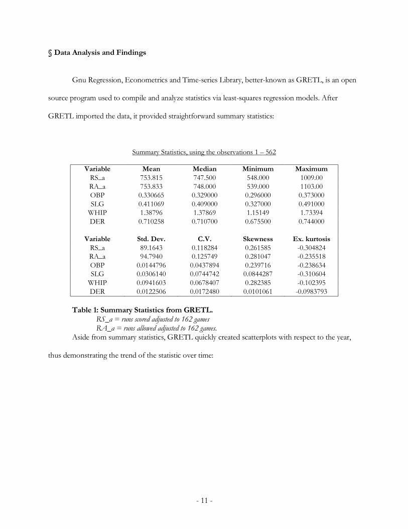
Figure 1: Scatterplot of Runs (Adjusted) versus Year

As one can see, there has been a gradual increase in run production from 1986 to 2005.

However, it is uncertain whether this increase is due to the improved abilities of hitters or the

decreased abilities of pitchers and fielders. To visually check this, scatterplots of OBP, SLG, WHIP

and DER can be constructed to view the trend:

- 13 -

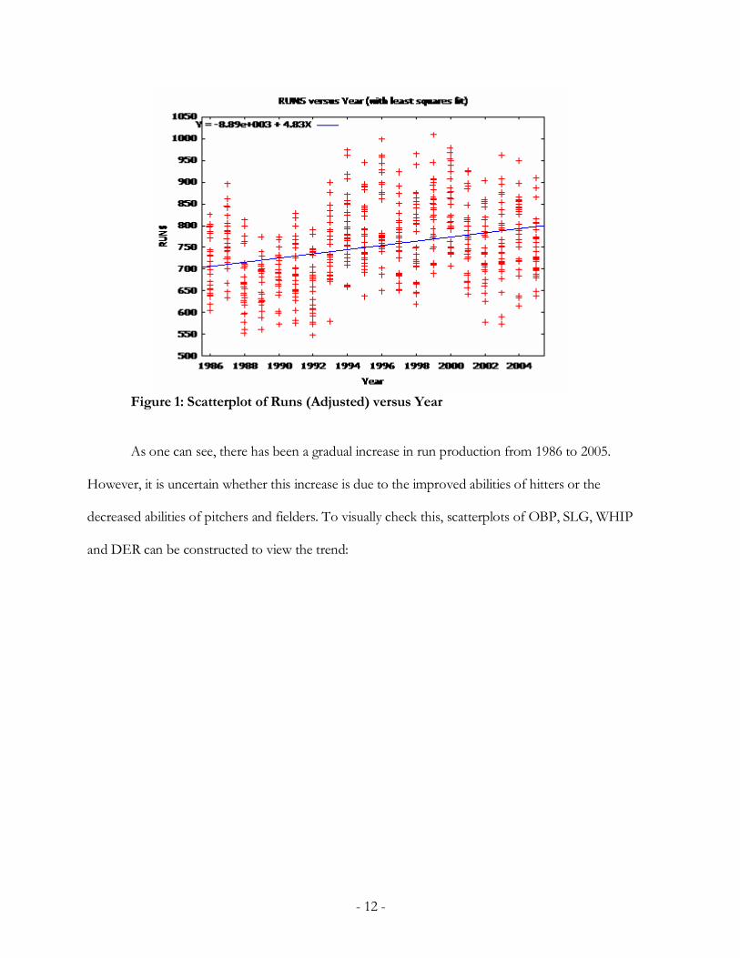
Figure 2: Scatterplot of OBP versus Year

Figure 3: Scatterplot of SLG versus Year

Offensive output has seemingly had a significant gradual increase, with a jump between the

years of 1993 and 1994, especially with power (slugging percentage).

- 14 -

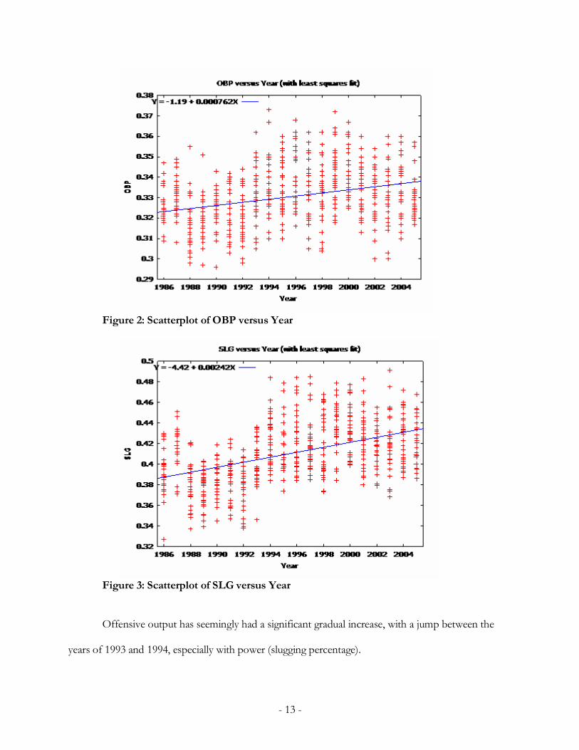
Figure 4: Scatterplot of WHIP versus Year

Figure 5: Scatterplot of DER versus Year

- 15 -

Pitching seems to have remained stable, as WHIP has increased only very little, but fielding

ability has dipped during the past twenty years. Despite the number of homeruns increasing since the

late 1990s, possibly due to the Steroid Era in baseball (which is being resolved), DER has decreased,

where an increase in homers should cause the DER to increase as well.

To truly test the hypothesis of this thesis, GRETL can construct ordinary least-squares

regression planes and their corresponding equations, correlation coefficients, and other helpful

statistical tests to verify the offensive model:

Model 1: OLS estimates using the 562 observations 1-562 Dependent variable: RS_a

Variable Coefficient Std. Error t-statistic p-value significance

const -849.805 27.448 -30.9605 < 0.00001 *** OBP 2918.72 128.515 22.7111 < 0.00001 *** SLG 1553.26 60.7843 25.5536 < 0.00001 ***

Mean of dependent variable = 753.815 Standard deviation of dep. var. = 89.1643 Sum of squared residuals = 407849 Standard error of residuals = 27.0112 Unadjusted R2 = 0.908556 Adjusted R2 = 0.908229 F-statistic (2, 559) = 2777.02 (p-value < 0.00001) Log-likelihood = -2648.43 Akaike information criterion = 5302.87 Schwarz Bayesian criterion = 5315.86 Table 2: OLS Estimates of Runs Scored (Adjusted) versus OBP and SLG

The best-fitting model results in a very good fit, according to the significance of the variables

and the strong, positive correlation coefficient. As expected, the model suggests that on-base

percentage and slugging percentage have direct positive effects on runs scored; the higher the OBP

or SLG, the higher the runs scored. In addition, an F-statistic with a low p-value suggests that none

of the variables (OBP and SLG) can be omitted when computing the regression plane:

- 16 -

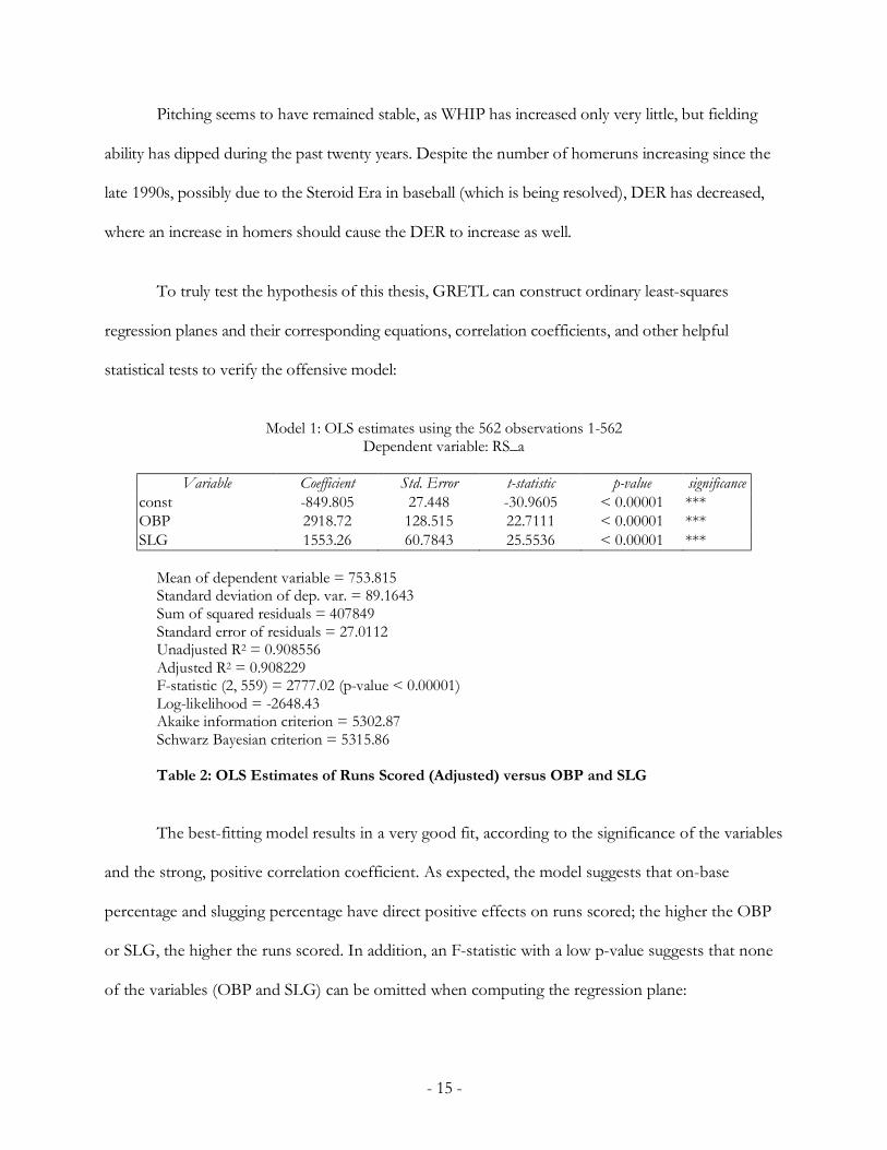
Figure 6: Fitted, Actual Plot of Runs Scored (Adjusted) versus OBP and SLG

Visually, regression planes, in three-dimensions, are much easier to grasp, whereas regression

models with more than two input variables cannot be graphed. GRETL allows the three-

dimensional figure to be rotated, and the image above optimally portrays the plane in space such

that the axes are easily visible while the actual values can be seen relative to the regression plane.

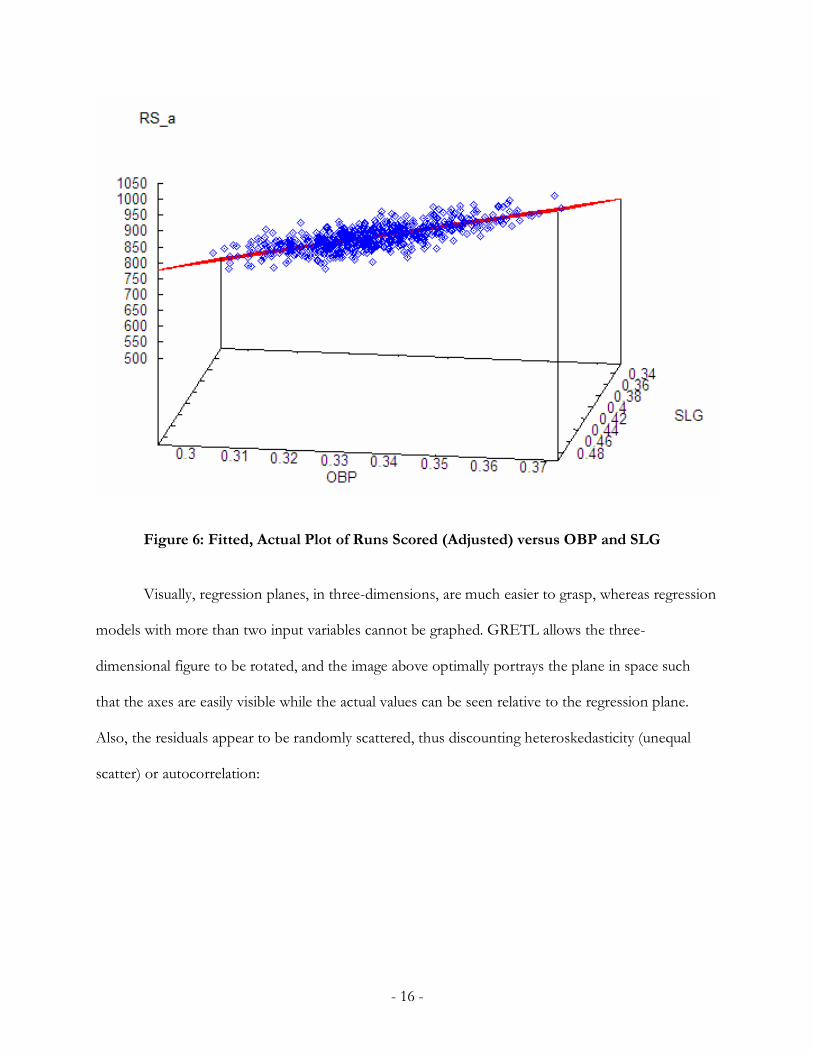
Also, the residuals appear to be randomly scattered, thus discounting heteroskedasticity (unequal

scatter) or autocorrelation:

- 17 -

Figure 7: Residuals for Runs Scored (Adjusted) Regression Model

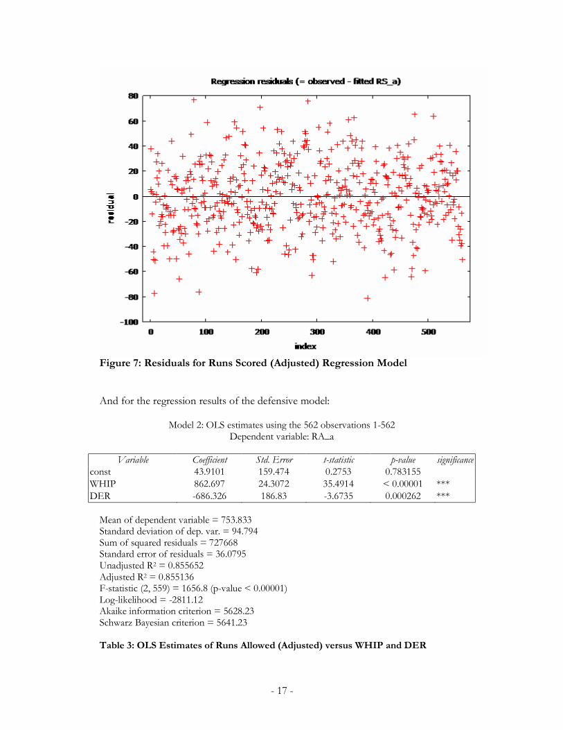
And for the regression results of the defensive model:

Model 2: OLS estimates using the 562 observations 1-562 Dependent variable: RA_a

Variable Coefficient Std. Error t-statistic p-value significance

const 43.9101 159.474 0.2753 0.783155 WHIP 862.697 24.3072 35.4914 < 0.00001 *** DER -686.326 186.83 -3.6735 0.000262 ***

Mean of dependent variable = 753.833 Standard deviation of dep. var. = 94.794 Sum of squared residuals = 727668 Standard error of residuals = 36.0795 Unadjusted R2 = 0.855652 Adjusted R2 = 0.855136 F-statistic (2, 559) = 1656.8 (p-value < 0.00001) Log-likelihood = -2811.12 Akaike information criterion = 5628.23 Schwarz Bayesian criterion = 5641.23 Table 3: OLS Estimates of Runs Allowed (Adjusted) versus WHIP and DER

- 18 -

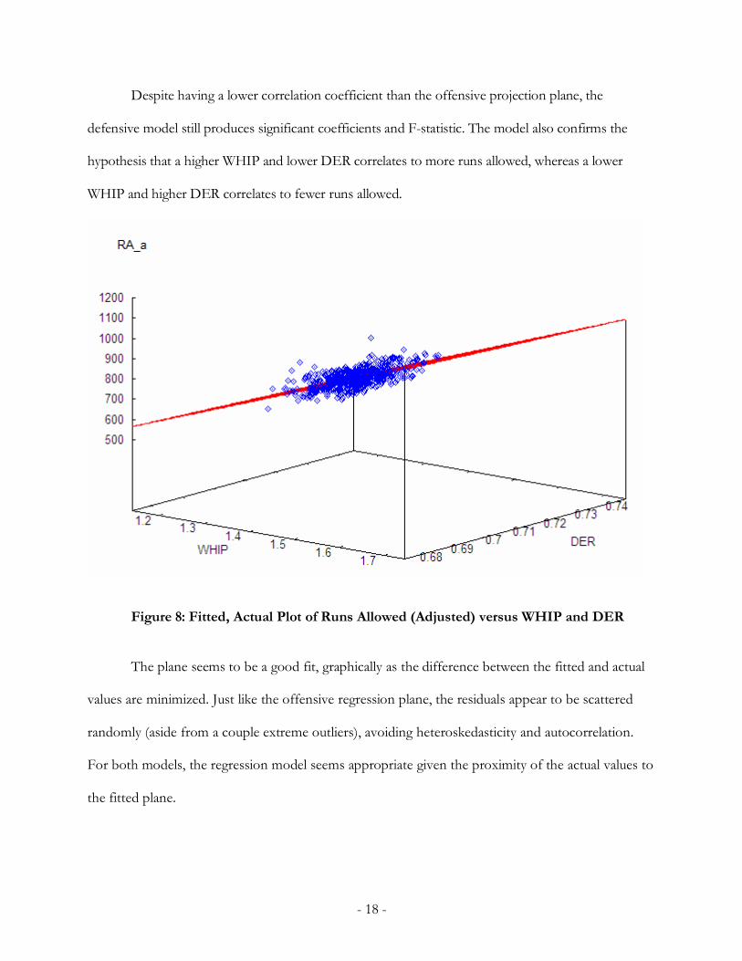
Despite having a lower correlation coefficient than the offensive projection plane, the

defensive model still produces significant coefficients and F-statistic. The model also confirms the

hypothesis that a higher WHIP and lower DER correlates to more runs allowed, whereas a lower

WHIP and higher DER correlates to fewer runs allowed.

Figure 8: Fitted, Actual Plot of Runs Allowed (Adjusted) versus WHIP and DER

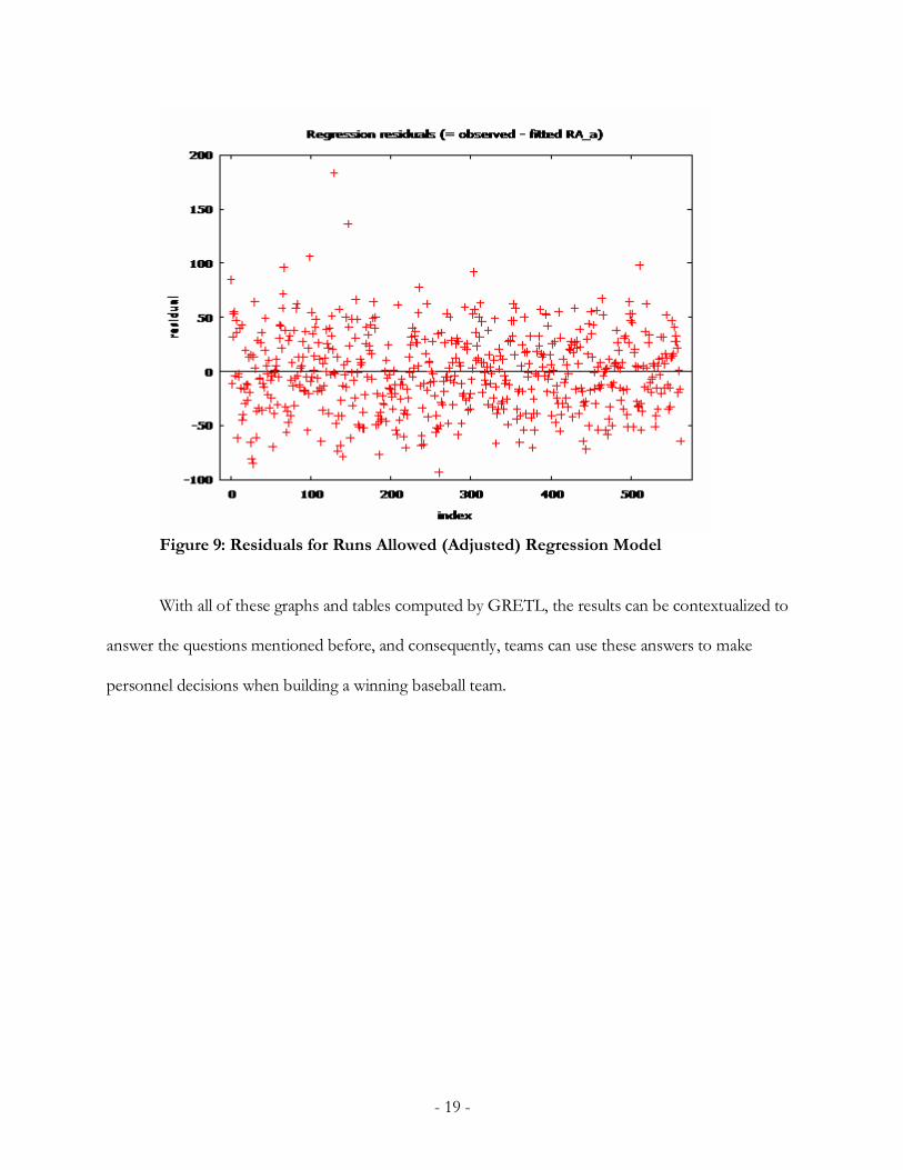
The plane seems to be a good fit, graphically as the difference between the fitted and actual

values are minimized. Just like the offensive regression plane, the residuals appear to be scattered

randomly (aside from a couple extreme outliers), avoiding heteroskedasticity and autocorrelation.

For both models, the regression model seems appropriate given the proximity of the actual values to

the fitted plane.

- 19 -

Figure 9: Residuals for Runs Allowed (Adjusted) Regression Model

With all of these graphs and tables computed by GRETL, the results can be contextualized to

answer the questions mentioned before, and consequently, teams can use these answers to make

personnel decisions when building a winning baseball team.

- 20 -

§ Discussion of Results

Without a doubt, run production has increased steadily in the past twenty years. As the

previous scatterplots highlighted, OBP and SLG (the two clear gauges for offensive efficiency) both

have climbed in the recent past while WHIP has correspondingly increased as well. However, this can

be due to the fact that OBP and WHIP are inverses—OBP is the ability to become a base runner,

while WHIP is the number of base runners allowed per inning. The gradual decrease in DER seems

completely independent of the other three statistics.

There have been several, popular theories that attempt to explain these changes in baseball.

The most logical proposal attributes the increase in offensive production to baseball’s expansion from

26 to 30 teams between 1986 and 2005. As there are 25 players per team roster, this means that there

were 100 more fringe major league-level players in 2005 than 1986. Also, weak hitters can be hidden

on the team’s bench, used in fill-in situations or when the game is already decided. In contrast

however, the better pitchers are physically unable to pitch every inning of every game, so in order to

compensate for the lost innings, the pitchers among the 100 extra fringe players would have filled

those innings. Consequently, worse pitchers facing better hitters naturally inflates run output, which

legitimizes the upward trends of OBP, SLG and WHIP. As for the decrease in DER, an explanation

for this can be rooted on the more recent emphasis on offensive skills in lieu of defensive ability. In

other words, gone are the days of the slick-fielding middle infielders (shortstops and second basemen)

who have sub-par batting averages. General managers are favoring such middle infielders that can hit

as well as the more traditional power positions (first basemen, third basemen, and corner outfielders)

who sacrifice fielding ability for offensive prowess.

- 21 -

Aside from the expansion theory, other suggestions for offensive inflation include rumors of

Major League Baseball executives authorizing juiced balls—baseballs that are more tightly wound at

their seams, which would cause them to carry a longer distance. Also, pitchers have opined that the

strike zone, which is interpreted independently by different umpires, has generally shrunken; this

forces pitchers to pitch around the plate more, thus providing batters with better chances to make

solid contact. The most recent and popular theory attributes offensive inflation to steroids and

performance-enhancing drugs. For years, the players’ union’s collective bargaining agreement

prohibited drug testing by the league, which essentially allowed the players to use and/or abuse any

drug without the threat of punishment. With this in mind, there is almost no doubt that a significant

percentage of players abused steroids in order to improve their performance on the field, including all-

stars that have been subjugated to a grand jury investigation in 2003 whose after-effects have forced

Congress to intervene. For example, Barry Bonds, who has been under the most scrutiny recently, saw

his yearly homerun count jump in 2000 and peak at a record-setting 73 homeruns in 2002, despite

arguably playing after his prime into his late 30s and early 40s. As steroid distributors like Victor Conte

and Greg Anderson underwent prison time for supplying steroids to athletes including baseball

players, consequently in 2005, Major League Baseball imposed progressively harsh suspension

penalties upon failure of random drug tests to eradicate steroids from the sport. No matter what

theory is proposed, the data do not lie, since the trends have suggested that offense has increased in

the past twenty years.

The fitted model for offensive production refutes both Paul DePodesta and traditional

sabermetricians to certain degrees. As mentioned before, Paul DePodesta argued in an interview in

Moneyball that OBP was three times as important as SLG, and traditional sabermetricians, by simply

creating the OPS statistic (OBP + SLG) inherently value OBP and SLG as equals. But the equation

- 22 -

for the regression plane, as shown in Table 2, yields coefficients of 2918.72 and 1553.26 for OBP and

SLG, respectively. This implies that OBP is roughly twice as important as SLG, when used to measure

offensive production through runs. The plane projects that a .001 increase in OBP adds approximately

3 runs of offense, whereas a .001 increase in SLG only adds 1.5 runs. The model falls in between Paul

DePodesta’s argument and the proposal of more traditional sabermetricians. In addition, the high

correlation coefficient, meaning that the proportion of the amount of variance in runs scored that can

be explained by OBP and SLG, is 0.908. A correlation coefficient of 1 suggests strict dependence.

With this in mind, the regression plane lends itself as a very good fit in estimating runs scored. The

more often a team’s players can get on-base (high OBP), coupled with the ability to drive them in with

power (SLG) should provide that team with a healthy amount of runs scored. Logically, OBP should

have more weight than SLG. For instance, if a team is able to load the bases with runners and then hit

a homerun, the grand slam would score four runs. But if a team cannot get runners on base before the

homerun, the solo homerun would score only one run; in other words, OBP precedes SLG when

scoring.

Obviously, there are other facets to offense in baseball that have been omitted in this relatively

simple three-dimensional model. Statistics such as stolen bases and sacrifice hits should not be ignored

in an offensive strategy. However, they were left out of the presented offensive model in order to

restrict the number of independent variables to two. By doing this, the model remains graphical (in

three dimensions with a plane) and thus easier to grasp for the less statistically-inclined. In addition, by

adding more variables, the correlation coefficient becomes artificially inflated in a regression model. As

for removing either of the two variables (OBP and SLG) from the proposed model, the Wald test and

consequent F-statistic argue against omitting either variable. The residual plot appears random enough

- 23 -

to discount serial correlation or heteroskedasticity—this result pushes for more support of the

proposed offensive model.

The second model was initially built based on earned-run average (ERA) and fielding

percentage, both of which are common measurements of pitching ability and defensive prowess;

however, this preliminary hypothesis was dropped immediately as the dependent variable, runs

allowed, is directly influenced by ERA. Also, fielding percentage only measures the proportion of

errors to assists and putouts. In lieu of ERA and fielding percentage, WHIP and defensive efficiency

rating (DER) provide accurate gauges of pitching and defensive abilities, respectively. Another reason

why these two measures are better suited is that they are independent of each other. WHIP is rooted

into pitching alone—it is the measure of a pitcher’s ability to keep runners off the basepaths, and if

there are no base runners, no runs can score. DER is a measure of the team’s defensive ability to

convert any balls put into play into outs, which is not influenced by the pitcher’s ability to prevent

runners from reaching base. Accordingly, one would expect runs allowed to increase as WHIP

increases and as DER decreases.

The model confirms this hypothesis as detailed in Table 2. The coefficient for WHIP is about

863, meaning a one-hundredth increase in WHIP allows 8.6 more runs over the course of the season,

while the coefficient for DER is -686, which suggests that a one-hundredth increase in DER takes

away 6.7 more runs over the course of the season. It is evident that keeping a low WHIP and a high

DER would limit the number of runs allowed. The model’s correlation coefficient of 0.855, despite

not being as strong as the offensive model’s correlation coefficient, still suggests that it can predict

runs allowed accurately. The less often a team’s pitchers allow the opponent to reach base, coupled

with a high proportion of turning balls put in play into outs would impair the opponent’s offensive

prospects.

- 24 -

The defensive regression plane’s residuals appear to be random as well, again discounting

heteroskedasticity and autocorrelation. The F-statistic through the Wald test does not suggest omitting

either WHIP or DER in the model. Unlike the offensive model, there are only a few more statistics,

mostly pitching ones that can be considered in constructing the plane. Strikeouts are conspicuously

absent though, as this model assumes strikeouts are equivalent to any other kind of out—groundout or

flyout. At times, a groundout or flyout can be more productive in scoring runs by advancing runners,

by way of a fielder’s choice or sacrifice bunts or fly balls. However, this factor may be offset by the

volume of double plays turned—in other words, a strikeout in this situation only results in one out,

whereas a double play yields two outs, further dampening the chance to score in that inning.

Although both models are reasonably good fits to predict runs scored and allowed, it is

impossible to completely find the perfect combination of variables. There is a certain luck factor

involved in the game—in a 162 game season, anything can happen; the league’s worst team can

surprise the league’s best team and win a three-game series. Also, Bill James argued that almost all one-

run games rely on luck. For instance, if a team strings together three hits in one inning and scores one

run, while its opponent racks up ten hits over the duration of the game but fail to score, the team that

had worse offensive output and defensive ability for that game wins 1-0. Because of this, the

correlation coefficients that were borne from both models, since they are reasonably close to 1, should

be adequate in suggesting the sufficiency of the two regression planes.

- 25 -

§ Conclusion and Extensions

Some might say that the models above are common sense—that it is logical to predict

offensive production from a team’s capacity to reach base and to drive runners home to score and to

predict defensive aptitude from the ability to prevent runners from getting on base and recording outs

when the ball is hit into play. However, many baseball fans and pundits still heavily lean on statistics

that fail to accurately describe a player or team’s abilities—batting average, runs batted in, earned-run

average, and fielding percentage. These statistics are too basic albeit very simple to compute, which is

probably why they are so frequently broadcasted. The significance of the high correlation coefficients

will hopefully convince a portion of the baseball masses that there are baseball statistics out there aside

from the mundane that are very useful and powerful in describing a player or his team. Perchance,

statistics such as OBP, SLG, WHIP, and DER will someday become mainstream—OBP has grown

popular because of Moneyball while SLG and WHIP are making headway in the media. However, DER

is still a mystery to many, despite being a great measure of a team’s skill in converting balls put into

play into outs, thus prohibiting the opponent to score.

This model has already established the weights of importance to the four above-mentioned

statistics in offensive and defensive contexts, but what can this model extend to? Returning to Bill

James’ Pythagorean Percentage, where the formula is:

%( )

RunsScoredWinRunsScored RunsAllowed

α

α α=+

Originally, the exponent that was used was two, which resembled the traditional Pythagorean

equivalence for right triangles. However, as mentioned before, this exponent has been adjusted to

- 26 -

approximately 1.8. Now, if the regression models from before are plugged into the Pythagorean

model:

(2918.72*OBP+1553.26*SLG-849.91)%(2918.72*OBP+1553.26*SLG-849.91) (862.70*WHIP-686.33*DER+43.91)

Winα

α α=+

Using this model and its corresponding partial derivatives:

%WinOBP

∂∂

, %Win

SLG∂∂

, %Win

WHIP∂∂

, and %Win

DER∂∂

can determine the precise value of each of the

variables and how their changes would affect team winning percentage. The quotient rule for simple

calculus can be used to find the partial derivatives and its numerical value can actually be computed.

Thus, one can observe the change in winning percentage due to an incremental change in any of the

four other statistics. In addition, OBP, SLG, and WHIP are statistics that can be individualized; that is,

individual players have these measures themselves. Because of this, a general manager for a baseball

team, upon deciding whether to add or subtract a certain player from the team, can gauge the change

in the team’s OBP, SLG, or WHIP and its corresponding effect on winning percentage. Unlike the

three other statistics, DER fails to trickle to the individual level—a certain player’s defensive ability is

usually measured through errors, assists, put-outs and the consequential fielding percentage. However,

there are new statistics such as zone ratio (ZR) and range factor (RF) that can describe a defensive

player. These measures are still relatively subjective, but are definitely more objective than a scout’s eye

which is still useful for instances such as gauging player’s arm strength, which is immeasurable for non-

pitchers when playing defense. Perhaps this is what the future holds for the ongoing battle between

traditional scouts and statistical analysis; statistical analysis can confirm a scout’s opinions or a scout’s

observations can confirm statistical analysis. There can be a fine line or balance such that both sides

work together to optimally judge a player and his impending value for his team.

- 27 -

The two models above are not meant to be revolutionary in the world of sabermetrics; but

coupled with the Pythagorean percentage, they should be able to influence player personnel decisions.

The regression models are restricted to two inputs each, so that the results can be graphed and more

easily interpreted, even for the non-statistically inclined. The planes are accurate fits that should not be

ignored when evaluating talent with statistical analysis. Hopefully, OBP, SLG, WHIP, and DER will

not only become mainstream statistics, replacing those that are just too basic to accurately measure

ability, but become the statistics of choice when judging a player or team’s offensive and defensive

skills.

- 28 -

APPENDIX

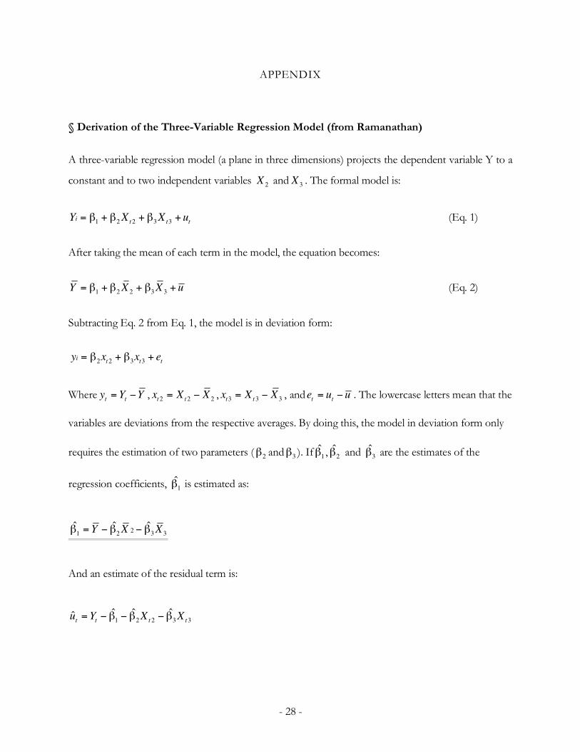
§ Derivation of the Three-Variable Regression Model (from Ramanathan)

A three-variable regression model (a plane in three dimensions) projects the dependent variable Y to a

constant and to two independent variables 2X and 3X . The formal model is:

1 2 2 3 3i t t tY X X uβ β β= + + + (Eq. 1)

After taking the mean of each term in the model, the equation becomes:

1 2 2 3 3Y X X uβ β β= + + + (Eq. 2)

Subtracting Eq. 2 from Eq. 1, the model is in deviation form:

2 2 3 3i t t ty x x eβ β= + +

Where t ty Y Y= − , 2 2 2t tx X X= − , 3 3 3t tx X X= − , and t te u u= − . The lowercase letters mean that the

variables are deviations from the respective averages. By doing this, the model in deviation form only

requires the estimation of two parameters ( 2β and 3β ). If 1̂β , 2β̂ and 3β̂ are the estimates of the

regression coefficients, 1̂β is estimated as:

21 2 3 3ˆ ˆ ˆY X Xβ β β= − −

And an estimate of the residual term is:

1 2 2 3 3ˆ ˆ ˆˆt t t tu Y X Xβ β β= − − −

- 29 -

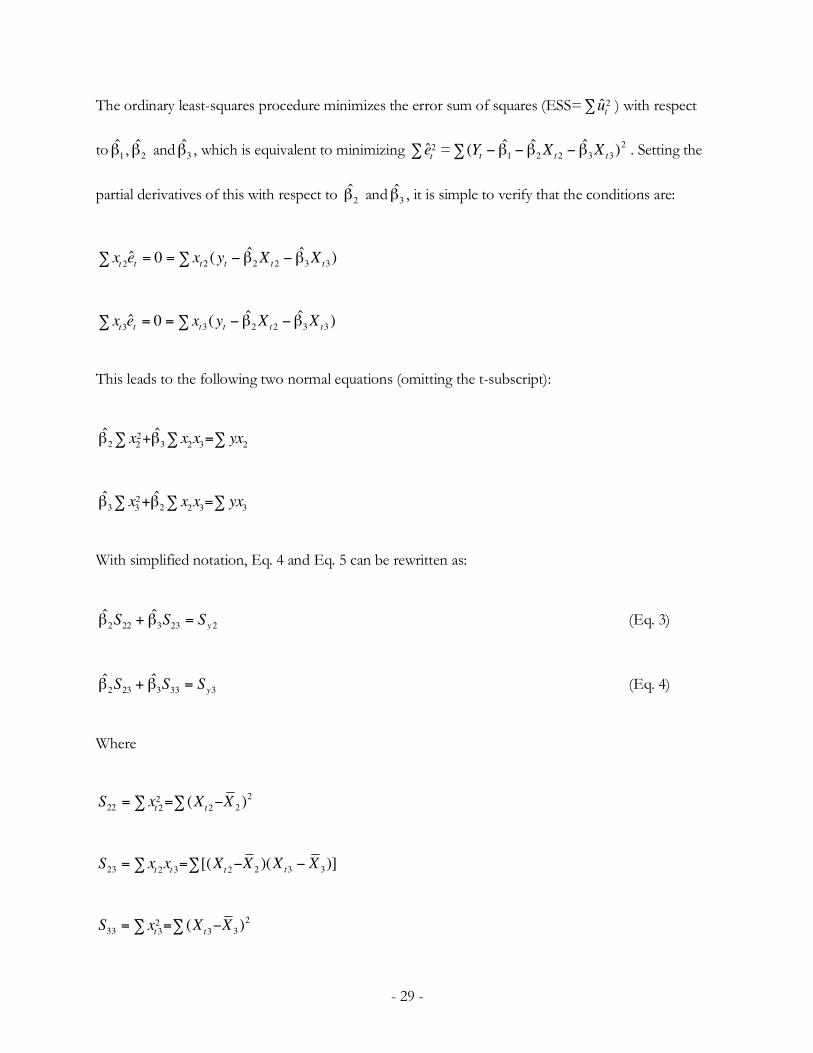
The ordinary least-squares procedure minimizes the error sum of squares (ESS= 2t̂u∑ ) with respect

to 1̂β , 2β̂ and 3β̂ , which is equivalent to minimizing 2t̂e∑ = 2

1 2 2 3 3ˆ ˆ ˆ( )t t tY X Xβ β β− − −∑ . Setting the

partial derivatives of this with respect to 2β̂ and 3β̂ , it is simple to verify that the conditions are:

2 2 2 3 32ˆ ˆˆ 0 ( )t t t t ttx e x y X Xβ β= = − −∑ ∑

3 2 2 3 33ˆ ˆˆ 0 ( )t t t t ttx e x y X Xβ β= = − −∑ ∑

This leads to the following two normal equations (omitting the t-subscript):

22 32 2 3 2

ˆ ˆx x x yxβ β+ =∑ ∑ ∑

23 23 2 3 3

ˆ ˆx x x yxβ β+ =∑ ∑ ∑

With simplified notation, Eq. 4 and Eq. 5 can be rewritten as:

2 22 3 23 2ˆ ˆ

yS S Sβ β+ = (Eq. 3)

2 23 3 33 3ˆ ˆ

yS S Sβ β+ = (Eq. 4)

Where

2222 22 2( )t tS x X X= = −∑ ∑

23 2 3 32 3 2[( )( )]tt t tS x x X X X X= = − −∑ ∑

2233 33 3( )t tS x X X= = −∑ ∑

- 30 -

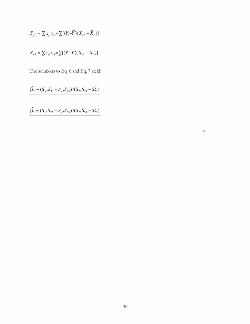
2 2 22 [( )( )]y tyt t tS x x Y Y X X= = − −∑ ∑

3 3 33 [( )( )]y tyt t tS x x Y Y X X= = − −∑ ∑

The solutions to Eq. 6 and Eq. 7 yield:

22 2 33 3 23 22 33 23

ˆ ( ) /( )y yS S S S S S Sβ = − −

23 3 22 2 23 22 33 23

ˆ ( ) /( )y yS S S S S S Sβ = − −

W

- 31 -

REFERENCES

JAMES, BILL (1985): The Bill James Historical Abstract. Villard Books.

ALBERT, JIM, AND JAY BENNETT (2003): Curve Ball. Copernicus Books.

SCHWARZ, ALAN (2004): The Numbers Game: Baseball’s Lifelong Fascination with Statistics. Thomas Dunne Books.

LEWIS, MICHAEL (2003): Moneyball: The Art of Winning an Unfair Game. W. W. Norton & Co.

GOLDMAN, STEVEN (2006): “Can a Team Have Too Much Pitching?” Baseball Between the Numbers. Ed. Jonah Keri. Basic Books / Perseus Books Group. 272-291.

RICE, JOHN A. (1995): Mathematical Statistics and Data Analysis, Second Edition. Duxbury Press / Wadsworth Publishing Company.

RAMANATHAN, RAMU (2002): Introductory Econometrics with Applications, Fifth Edition. South-Western / Thomson Learning.

FORMAN, SEAN L.: Baseball-Reference.com – Major League Statistics and Information. http://www.baseball-reference.com/. (January 31, 2006).

FORMAN, SEAN L.: The Baseball Archive. http://www.baseball1.com/statistics/. (January 31, 2006).

COHEN, GARY: The Baseball Cube. http://www.thebaseballcube.com/. (January 31, 2006).

MAJOR LEAGUE BASEBALL: Major League Baseball: The Official Site. http://mlb.mlb.com/NASApp/mlb/index.jsp. (January 31, 2006).

ESPN.COM: Baseball Index. http://sports-att.espn.go.com/mlb/index. (January 31, 2006).

RETROSHEET, INC.: Retrosheet. http://www.retrosheet.org/. (January 31, 2006).