Embed Size (px)
Citation preview

R E
OC N
F I G
ICT Call 9
RECONFIG
FP7-ICT-600825
Deliverable D4.2:
Decentralized Adjustment and Verification Based on Sensor andSymbolic Information Exchange
February 26, 2015

D4.2 FP7-ICT-600825 RECONFIG February 26, 2015
Project acronym: RECONFIGProject full title: Cognitive, Decentralized Coordination of Heterogeneous
Multi-Robot Systems via Reconfigurable Task Planning
Work Package: WP4Document number: D4.2Document title: Decentralized Adjustment and Verification Based on Sen-
sor and Symbolic Information ExchangeVersion: 1.0
Delivery date: February 28, 2015Nature: ReportDissemination level: Public
Authors: Dimos Dimarogonas (KTH)Jana Tumova (KTH)Meng Guo (KTH)Dimitris Boskos (KTH)Alejandro Marzinotto (KTH)Michele Colledanchise (KTH)Petter Ogren (KTH)Danica Kragic (KTH)Anastasios Tsiamis (NTUA)Charalampos P. Bechlioulis (NTUA)Kostas J. Kyriakopoulos (NTUA)
The research leading to these results has received funding from the European Union SeventhFramework Programme FP7/2007-2013 under grant agreement no600825 RECONFIG.
2

Summary
This deliverable summarizes the achieved results in the verification of high-level tasks assignedat the local level to multi-agent systems and the adaptation of the corresponding plans in orderto meat communication constraints. The proposed framework also provides measures of highlevel performance since it takes into account uncertainty in the robots sensors and actuators andanalyzes the systems fault tolerance.
3

Chapter 1
Introduction
In this chapter, we introduce our approach to decentralized high-level task planning for multi-agentsystems with knowledge update based on sensor and symbolic information exchange. Our particularobjectives have been focused on the appropriate adjustment of the high-level specifications andplans in order to deal with robot action failures caused by imprecisions in sensors and actuators,and various communication constrains between agents of the multi-agent systems.
The specification and synthesis of structured and complex team behaviors is a highly activearea of research in the field of robotics. Particularly, Linear Temporal Logic (LTL) formulas serveas suitable descriptions of the desired high-level goals. LTL allows to rigorously specify varioustemporal tasks, including periodic surveillance, sequencing, request-response, and their combina-tions. Furthermore, it has some resemblance to natural language and in recent years, it showed apotential to express complex robotic tasks. With the use of formal verification-inspired methods, adiscrete plan that guarantees the specification satisfaction can be automatically synthesized, whilevarious abstraction techniques bridge the continuous control problem and the discrete planningone. As a result, a generic hierarchical approach that allows for correct-by-design control withrespect to the given LTL specification has been formulated and largely employed during the lastdecade or so in single-agent as well as multi-agent settings [22, 28, 38, 55, 68, 69, 80, 93, 97].
We focus on a multi-agent version of the LTL planning problem, where each agent is given anindividual task. As also highlighted in D4.1 the solution to the planning problem is decomposed ina three step hierarchical approach. First, the robot in its environment is abstracted into a finite,discrete state-transition structure. Second, a discrete plan that satisfies the temporal logic task issynthesized and third, the plan is implemented by a correct-by-design continuous controller.
The organization of the main part of this chapter is as follows. In Section 1.1 we provide ashort description of our objectives and approach, we discuss related work in Section 1.2 and weoutline the structure of the rest of this report in 1.3.
1.1 Our Objectives and Approach
Our particular objectives are the following and the details together with our solution approach areprovided in Sec. 1.1.1,1.1.2, 1.1.3 and 1.1.4, respectively:
(i) Reactive robot action planning from high-level LTL specifications with feedback to actionfailures;
4

D4.2 FP7-ICT-600825 RECONFIG February 26, 2015
(ii) Decentralized multi-agent LTL planning, control, and plan adjustment under coupled con-straints;
(iii) Multi-agent LTL task execution with knowledge updates provided solely though implicitcommunication; and
(iv) Multi-robot task coordination and fault tolerance analysis.
1.1.1 Reactive Robot Action Planning from LTL Specifications
We consider the action planning problem from LTL specifications for a single robot whose statesand action capabilities are captured through a finite transition system. Our aim is to enhance thetemporal logic specification of “where to go” with “what to do” there and to propose a frameworkthat 1) bridges the high-level plan with the low-level motion, grasping, and other controllers, 2) ismodular and extensible to handle different robots and their capabilities, 3) is reactive and able tocope with the unreliability of the robot’s sensors and actuators leading to failures of its actions,and 4) guarantees that the temporal logic task is met as closely as possible.
In our approach, we use a surveillance fragment of the state-event variant of linear temporallogic (SE-LTL) [14,85] allowing for requirements and restrictions on both the robot’s locations andits actions. At the high-level planning layer, we propose an algorithm to synthesize a maximallysatisfying discrete control strategy while taking into account that the robot’s action executionsmay fail. Our framework is based on defining a quantitative metric to measure the level ofnoncompliance of a robot’s behavior with respect to the given SE-LTL formula and we synthesizea maximally satisfying discrete, reactive control strategy in the form of an Input/Output (I/O)automaton. We consider a specific kind of nondeterminism that we handle algorithmically whileemploying ideas from synthesis for deterministic systems.
1.1.2 Decentralized Multi-Agent LTL Control Under Coupled Constraints
In our second objective, we consider a team of agents modeled as a dynamical system thatare assigned local task specifications through LTL formulas. The agents might not be able toaccomplish the tasks by themselves and hence requirements on the other agents’ behaviors arealso part of the LTL formulas. Consider for instance a team of robots operating in a warehousethat are required to move goods between certain warehouse locations. While light goods can becarried by a single robot, help from another robot is needed to move heavy goods. We aim atfinding motion controllers and action plans for the agents that guarantee the satisfaction of allindividual LTL tasks. We seek for a decentralized solution while taking into account the constraintthat the agents can exchange messages only if they are close enough. This constraint triggers theneed for the constant adjustment of the individual agents’ controllers in reaction to the collectiveteam behavior.
We follow the hierarchical approach to LTL planning, by first generating for each agent asequence of actions as a high-level plan that, if followed, guarantees the accomplishment of therespective agent’s LTL task. For the continuous controller design we propose a solution based ona decentralized coordination scheme through a dynamic leader re-election, which guarantees thelow-level connectivity maintenance and a progress towards the satisfaction of each agent’s task.
5

D4.2 FP7-ICT-600825 RECONFIG February 26, 2015
1.1.3 LTL Task Execution under Implicit Communication
This objective is motivated by the following scenario which includes a team of robots that areassigned a high-level complex goal each and have to collaborate to execute them (for instance,to collaboratively carry a heavy object). At the same time, the robots do not have the abilityto communicate explicitly with each other at all and hence, they cannot learn the goals of theother team members. Our aim is to control the team so that each of the given high-level goalsis reached, in a decentralized way and without employing and explicit inter-robot communication.We introduce the first step towards addressing this challenging problem and focus on the task ofcooperative manipulation, where two robots collaborate in order to carry a heavy object. Theirindividual goal specifications, such as periodic surveillance of a certain set of regions, are givenas two individual LTL formulas. We aim to replace explicit with implicit communication that isyielded indirectly from the interaction of the robots via the common holding object.
Our approach relies on a decentralized protocol that translates the aforementioned interactioninto robot (motion) intentions and subsequently employs them in the control design, which weintroduce in details in Deliverable D3.3. For LTL task execution, we leverage the fact thatunder implicit communication, the two agents can perform (i) A-to-B motion in a leader-followerformatioin and (ii) dynamic leader switch. We propose a leader re-election strategy that guaranteesthe fulfillment of both individual goal specifications.
1.1.4 Multi-Robot Task Coordination and Fault Tolerance
In our final objective, we first consider a team of agents and assume that there is no pre-specifiedglobal task and individual task specifications are assigned locally to each agent as LTL formu-las [28], [37], [93]. Moreover, these local tasks are dependent in the sense that one agent may needothers’ collaboration to fulfill its own task. Thus, coordination is crucial for the accomplishmentof all local tasks. The greatest challenge of task coordination for multi-agent systems under de-pendent local tasks is the computational complexity which leads to a computational time blowupin centralized solutions. We aim to propose a bottom-up distributed scheme which guarantees thesatisfaction of each individual task under the assumption that these tasks are mutually feasible.With respect to fault tolerance analysis we focus on multi-robot missions which rely on BehaviorTree (BT) controllers. Our aim is to extend the single robot BT (controllers) to a multi-robot BTin order to improve performance and fault tolerance of the multi-robot system.
In our approach to the first part of the objective, we focus on dependent local task specifica-tions, specified as co-safe LTL formulas. We propose a distributed bottom-up solution which relieson the offline initial plan synthesis, the design of an on-line request and reply messages exchangeprotocol and the synthesis of a real-time plan adaptation algorithm. Our approach to the secondpart of this objective, namely extending the single robot BT to a multi-robot BT, enables us tocombine the fault tolerant properties of the BT, with the fault tolerance inherent in multi-robotapproaches. Furthermore, we improve performance by identifying and taking advantage of theopportunities of parallel task execution, that are present in the single robot BT.
6

D4.2 FP7-ICT-600825 RECONFIG February 26, 2015
1.2 Related Work
Reactive Temporal Logic Planing
Related work focused on techniques for reactive temporal logic planning include e.g., studyingsynthesis for nondeterministic systems [56, 99] or general-reactivity goals [60], a receding horizonapproach to synthesis [102], or synergistic interface between a planner and a controller [9]. Otherrelated works aim at planning under unsatisfiable temporal logic specifications, such as [13,70,95],where the authors focus on least-violating planning with respect to a proposed metric. Theyfind, according to a proposed metric, the maximal part of the specification that can be satisfiedby the model, and they generate the corresponding controller for this part of the specification.Other authors [36, 54] propose to systematically revise the given temporal logic specification tobe satisfiable by the given model and close to the original formula.
Control of Multi-Agent Systems under LTL Tasks
Multi-agent planning under temporal logic tasks has been studied in several recent papers [16,37,48,55,68,78,93,97,98]. Many of them build on top-down approach to planning, when a single LTLtask is given to the whole team. For instance, in [16,97], the authors propose decomposition of thespecification into a conjunction of independent local LTL formulas. Contrary, in the bottom-upapproach, each agent is assigned its own local task. The tasks can be independent [28, 38] orpartially dependent, involving requests for collaboration with the others [93]. A major researchinterest here is the decentralization of planning and control procedures. For instance, in [38], adecentralized revision scheme is suggested for a team in a partially-known workspace. In [28],gradual verification is employed to ensure that independent LTL tasks remain mutually satisfiablewhile avoiding collisions. Also, in [93], a receding horizon approach is employed to achieve partiallydecentralized planning for collaborative tasks and in [80], the authors propose a compositionalmotion planning framework for multi-robot systems under safe LTL specifications.
Cooperative Manipulation
The literature on cooperative manipulation involves many works that implement centralizedschemes [52,91]. Other works implement decentralized schemes, which however, depend on heavyexplicit communication via exchanging control signals, state measurements and desired trajecto-ries [53,89,90]. Decentralized works which make use of implicit communication include [58], [87].Both papers propose a leader-follower scheme, where the cooperating robots are nonholonomic.In [11] a pushing scenario is considered, where the leader is responsible for the steering angle, whilethe follower only pushes. A leadership exchange scenario among mobile robots is also exploredin [74].
Behavior Trees
BTs have become a recent alternative to Controlled Hybrid Systems (CHSs) for reactive faulttolerant execution of robot tasks. They were first introduced in the computer gaming industry[15,44,45], to meet their needs of modularity, flexibility and reusability in artificial intelligence forin-game opponents. Their popularity lies in its ease of understanding, its recursive structure, andits usability, creating a growing attention in academia [3,10,57,66,73,75,82]. BTs were first usedin [15,44], in high profile computer games, such as the HALO series. Later work merged machine
7

D4.2 FP7-ICT-600825 RECONFIG February 26, 2015
learning techniques with BTs’ logic [66, 75], making them more flexible in terms of parameterpassing [82]. The advantage of BTs as compared to a general Finite State Machines (FSMs) wasalso the reason for extending the JADE agent Behavior Model with BTs in [10], and the benefitsof using BTs to control complex missions of Unmanned Areal Vehicles (UAVs) was describedin [73]. In [57] the modular structure of BTs addressed the formal verification of mission plans.Additional details on BTs can also be found in the introduction of D4.1.
1.3 Report Outline
In the remainder of the report we present the results for each objective in a standalone chapter.
(i) Reactive robot action planning under LTL specifications is the topic of Chapter 2 andpresents results from our paper [94].
(ii) Decentralized multi-agent LTL planning in the presence of coupled constraints is providedin Chapter 3. The results are based on our paper [41].
(iii) Multi-agent LTL plan execution under implicit communication is studied in Chapter 4. Theresults are based on our work [92].
(iv) Finally, Chapter 5 covers multi-agent task coordination and fault tolerance analysis. Thecorresponding results are based on our work [39] and [18].
8
Chapter 2
Maximally Satisfying LTL Action Plan-ning
2.1 Introduction
In this chapter we focus on autonomous robot action planning problem from Linear TemporalLogic (LTL) specifications, where the action refers to a “simple” motion or manipulation task,such as “go from A to B” or “grasp a ball”. Our results aim at the high-level planning layerand we propose an algorithm to synthesize a maximally satisfying discrete control strategy whiletaking into account that the robot’s action executions may fail.
The problem addressed can be formulated as follows. Similarly as in some related literature(e.g., [36, 85, 99]) we assume that the robot’s states and action capabilities are at the highestlevel of abstraction captured through a finite, discrete transition system. Due to imprecisions inrobot’s sensors and actuators, each attempt to execute an action might result into a success ora failure. As the specification language, we use a surveillance fragment of the state-event variantof linear temporal logic (SE-LTL) [14, 85] allowing for requirements and restrictions on both therobot’s locations and its actions.
The chapter is organized as follows: In Sec. 2.2, we fix necessary preliminaries in transitionsystems, temporal logics and behavior trees. In Sec. 2.3, we formalize the problem and in Sec. 2.4we introduce the details of the proposed solution. We provide experimental results in Section 2.5and summarize in Section 2.6.
2.2 Preliminaries
2.2.1 Notation
Given a set S, let |S|, 2S, S∗ and Sω denote the cardinality of S, the set of all subsets of S, andthe set of all finite (possibly empty) and infinite sequences of elements of S, respectively. For aninfinite sequence s = s(1)s(2) . . . ∈ Sω, we denote by si the suffix of s beginning in s(i). Given afinite sequence sfin and a finite or an infinite sequence s, we denote by sfins their concatenation andby sωfin the infinite word sfinsfinsfin . . .. Furthermore, the concatenation of a set of finite sequencesSfin , and a set of finite or infinite sequences S, is Sfin · S = sfins | sfin ∈ Sfin , s ∈ S.
9

D4.2 FP7-ICT-600825 RECONFIG February 26, 2015
2.2.2 Transition System, Linear Temporal Logic, and Automata
Definition 1 (Transition System). A labeled transition system (TS) is a tuple T = (S, sinit ,Σ,→,Π, L), where S is a finite set of states; sinit ∈ S is the initial state; Σ is a finite set of events(or actions); →: S × Σ × S is a transition relation; Π is a set of atomic propositions, suchthat Σ∩Π = ∅; and L : S → 2Π is a labeling function that assigns to each state s ∈ S exactlythe subset of atomic propositions L(s) that hold true in there.
For convenience, we use sσ−→ s′ to denote the transition (s, σ, s′) ∈→ from state s to s′
under action σ. The transition system T is deterministic if for all s ∈ S, σ ∈ Σ, there existat most one s′ ∈ S, such that s
σ−→ s′. A trace of T is an infinite alternating sequence ofstates and events τ = s1σ1s2σ2 . . . ∈ (S · Σ)ω, such that s1 = sinit and si
σi−→ si+1, for alli ≥ 1. A trace fragment is a finite subsequence τfin = siσi . . . sjσj ∈ (S · Σ)∗ of an infinitetrace τ = s1σ1 . . . σi−1siσi . . . sjσjsj+1 . . .. A trace τ = τpre(τsuf )ω is called a trace with aprefix-suffix structure; τpre is the trace prefix and τsuf is the periodically repeated trace suffix.The set of all traces of T and the set of all traces of all transition systems are denoted by T(T )and T, respectively. Analogously, Tfin(T ) and Tfin denote the set of all finite trace fragmentsof T and of all transition systems, respectively. A trace τ = s1σ1s2σ2 . . . of T produces a wordw(τ) = w(1)w(2) . . ., where w(i) = L(si) ∪ σi.
Definition 2 (Trace Fragments Distance).Given τfin = siσi . . . sjσj ∈ Tfin , and a subset of indexes I ⊆ i, . . . , j, the restricted tracefragment τfin|I is created by removing the states and actions labeled with indexes from I, i.e.,∀`k ∈ I, τfin|I = siσi . . . s`k−1σ`k−1s`k+1σ`k+1 . . . sjσj .
The distance between trace fragments τfin , τ′fin ∈ Tfin is dist(τfin , τ
′fin) = min(|I|+ |I ′|), s.t.
w(τfin|I) = w(τ ′fin|I′).
Intuitively, the distance dist(τfin , τ′fin) is the number of states and actions that have to be
removed from and added to τfin for it to produce the same word as τ ′fin .A (control) strategy Ω : (S ·Σ)∗ · S → Σ for T is a function that assigns to each trace prefix
followed with a state the next action to be executed. A trace s1σ1s2σ2 . . . is a trace under thecontroller Ω if for all i ≥ 1, it holds that σi = Ω(s1σ1 . . . si). If T is deterministic, then thereis only one trace under each Ω, and thus we talk about the trace as about the strategy itself. Afinite-memory control strategy is intuitively one, whose outputs depend only on last m states andactions. Such a strategy can be represented an input/output automaton.
Definition 3 (Input/Output Automaton). An input/output (I/O) automaton is a tuple I =(Q, qinit ,Σin ,Σout , δ), where Q is a finite set of states; qinit is the initial state; Σin is an inputalphabet; Σout is an output alphabet; and δ : Q × Σin → Q × Σout is a partial transitionfunction.
A run of an I/O automaton I over an input word ι1ι2 . . . ∈ Σωin is a sequence of states q1q2 . . .,
with the property that q1 = qinit , and ∀i ≥ 1, ∃oi ∈ Σout , such that δ(qi, ιi) = (qi+1, oi). Theoutput sequence of such a run is o1o2 . . ..
The I/O automaton I can serve as a finite-memory control strategy for a transition systemT = (S, sinit ,Σ,→,Π, L) as follows. Assume that Σin = S, and Σout = Σ. Then, the inputwords for I are state sequences of T and the output sequences are action sequences for T . Thetransition system T is controlled by I in the following way: Assume that s is the current stateof T , q is the current state of I, and δ(q, s) = (q′, a). Then q′ becomes the new current stateof I, and a state s′, such that s
a−→ s′ becomes the new current state of T . There might be
10

D4.2 FP7-ICT-600825 RECONFIG February 26, 2015
multiple states s′, such that sa−→ s′, in which case, one of them is chosen nondeterministically,
corresponding to the fact that the application of the action a may have several different effects.If there is no s′, such that s
a−→ s′ in T , then I is not a valid control strategy for T .
State/Event Linear Temporal Logic
To specify the robot’s goals, we will use state/event variant of LTL [14] that allows to capturerequirements on both the robot’s state or its location and the actions it executes.
Definition 4 (SE-LTL). Let us consider transition system T = (S, sinit ,Σ,→,Π, L). AState/Event Linear Temporal Logic (SE-LTL) formula φ over the set of atomic propositionsΠ and the set of events Σ is defined inductively as follows:
1. every π ∈ Π and every σ ∈ Σ is a formula, and
2. if φ1 and φ2 are formulas, then φ1 ∨ φ2, ¬φ1, Xφ1, φ1 Uφ2, Gφ1, and Fφ1 are eachformulas,
where ¬ (negation) and ∨ (disjunction) are standard Boolean connectives, and X, U, G, andF are temporal operators.
Informally speaking, the trace τ = s1σ1 . . . of T satisfies the atomic proposition π if π issatisfied in s1 and the event σ if σ1 = σ. The formula Xφ states that φ holds in the followingstate, whereas φ1 Uφ2 states that φ2 is true eventually, and φ1 is true at least until φ2 is true.The formulas Fφ and Gφ state that φ holds eventually and always, respectively. For the fullsemantics of SE-LTL, see [14].
The trace-satisfaction relation can be easily extended to satisfaction relation for words over2Π∪Σ. Particularly, a word w satisfies an SE-LTL formula φ over Π and Σ if there exists a traceτ ∈ T, such that τ |= φ and w = w(τ). The language of all words that satisfy φ is denoted byL(φ).
Buchi Automata
An alternative way to capture a property defined by an SE-LTL formula is a Buchi automaton.
Definition 5 (Buchi Automaton). A Buchi automaton (BA) is a tuple B = (Q, qinit,Υ, δ, F ),where Q is a finite set of states; qinit ∈ Q is the initial state; Υ is an input alphabet; δ ⊆Q× Σ×Q is a non-deterministic transition relation; and F is the acceptance condition.
The semantics of Buchi automata are defined over infinite input words over Υ. A run ofa BA B over an input word w = w(1)w(2) . . . is a sequence ρ = q1w(1)q2w(2) . . ., such thatq1 = qinit, and (qi, w(i), qi+1) ∈ δ, for all i ≥ 1. A run ρ = q1w(1)q2w(2) . . . is accepting ifit intersects F infinitely many times. A word w is accepted by B if there exists an acceptingrun over w. The language of all words accepted by B is denoted by L(B). A Buchi automatonis tight if and only if for all w ∈ L(B) there exists an accepting run q1w(1)q2w(2) . . . with theproperty that wi = wj ⇒ qi = qj . Any SE-LTL formula over Π and Σ can be translated into aBA with Υ = 2Π∪Σ, such that L(φ) = L(B) using standard techniques [14]. Furthermore, sometranslation algorithms (e.g., [34]), guarantee that the resulting BA is tight [81].
11
D4.2 FP7-ICT-600825 RECONFIG February 26, 2015
Graph Theory
Any automaton or transition system can be viewed as a graph G = (V,E) with the set of verticesV equal to the set of states, and the set of edges E given by the transition function in theexpected way. A simple path in G is a sequence of states vi . . . vl such that (vj , vj+1) ∈ E, for alli ≤ j < l, and vj = vj′ ⇒ j = j′, for all i ≤ j, j′ ≤ l. A cycle is a sequence of states vi . . . vlvl+1,where vi . . . vl is a simple path and vl+1 = vi. A weighted graph is a tuple G = (V,E,W ), whereW : E → N is a a function assigning weights to the edges. The length of a path vi . . . vl is thesum of its respective weights len(vi . . . vl) =
∑j∈i,...,l−1W (vj , vj+1). A shortest path from v to
v′ is a path minimizing its length and can be found efficiently using e.g., Dijkstra’s shortest pathalgorithm (see, e.g. [65]).
2.3 Problem Formulation and Approach
Our approach to the problem in this work builds on formal methods; we model the expected robot’saction capabilities as a transition system and the goal as an SE-LTL formula. The proposed solutionrelies on defining a quantitative metric to measure the level of noncompliance of a robot’s behaviorwith respect to the given SE-LTL formula and we synthesize a maximally satisfying discrete,reactive control strategy in the form of an Input/Output (I/O) automaton.
Similarly as in some related papers (e.g., [36, 85, 99]) we model the robot as a TS T =(S, sinit ,Σ,→,Π, L). The set of states S encode the possible states of the robot, such as itsposition in the environment, or the object it is carrying. The atomic propositions and the labelingfunction capture properties of interest of the robot’s states. The actions in Σ abstract the actionprimitives, such as “move from position A to position B”, or “grasp a ball” and the transitionfunction expresses the evolution of the robot’s states upon a successful execution of an actionprimitive. If the execution of an action fails, the robot stays at the same state. Formally, wedefine a success-deterministic transition system as the robot’s model.
Definition 6 (Success-deterministic Transition System).A success-deterministic transition system T is a syntactically deterministic transition systemwith specific nondeterministic semantics defined as follows: The traces of T are sequencess1σ1s2σ2 . . . and for each i ≥ 1 it holds that
• either siσi−→ si+1 (σi succeeds in si), or
• si = si+1, and ∃s′i+1, s.t. siσi−→ s′i+1 (σi fails in si).
Intuitively, the success-deterministic transition system has two possible outcomes for eachaction execution attempt. If the action succeeds, the transition is followed as expected; if it fails,the system’s state does not change.
The specification of the robot’s task takes a form of an SE-LTL formula φ. We specificallyfocus on recurrent tasks, that involve, e.g., periodic visits to selected regions of the environmentor repeated execution of certain actions. To pose the problem formally, we consider a specialsurveillance event σsur to be periodically executed. Intuitively, the execution of σsur indicatesthat the robot has finished a single surveillance cycle. The action σsur is available in Ssur ⊆ S,and for all s ∈ Ssur , the transition enabled by σsur is s
σsur−−→ s only. The attempt to execute theevent σsur is always successful. The SE-LTL formula φ is of form
φ = ϕ ∧ GFσsur , (2.1)
12

D4.2 FP7-ICT-600825 RECONFIG February 26, 2015
where ϕ is any SE-LTL formula over Π and Σ, such that σsur does not appear in ϕ. In otherwords, there are no other demands imposed on the execution of the surveillance event σsur apartfrom its infinite repetition, whereas arbitrary requirements and restrictions can be prescribed forthe other actions and atomic propositions.
Example 1. In Fig. 2.1 we give an example of a NAO robot’s workspace partitioned into 9regions; 6 rooms and 3 corridor regions. We assume the following set of action and motionprimitives Σ: r, b, l, t (move to the neighboring region on the right, bottom, left, or top, re-spectively), grab (grab a ball), drop (drop the ball), and σsur = light up. The robot’s stateis compound of the region the robot is present at and whether or not it holds a ball. Therobot is not allowed to cross a black line, and therefore the motion primitives r, b, l, t arenot enabled in all the states. Similarly, the action grab is enabled only in the set of regionsG ⊆ R1, . . . , R6, C1, . . . , C3, where an object to be grabbed is expected to be present. Ini-tially, the NAO is present in R1, with no object in its hand. The transition system model isT = (S, sinit ,Σ,→,Π, L), where
• S = R1, . . . , R6, C1, . . . , C3 × 1, 0; sinit = (R1, 0); Σ = r, b, l, t, grab, drop, light up; Π =R1, . . . , R6;
• (R1, 0)light up−−−−−→ (R1, 0); for all i ∈ 1, 2, 3, x ∈ 1, 0 : (Ci, x)
r−→ (Ci+1, x), (Ci+1, x)l−→ (Ci, x)
(Ri, x)b−→ (Ci, x), (Ci, x)
t−→ (Ri, x), (Ri+3, x)t−→ (Ci, x), (Ci, x)
b−→ (Ri+3, x), for all Ri ∈ G :
(Ri, 0)grab−−−→ (Ri, 1), for all i ∈ 1, . . . , 6 : (Ri, 1)
drop−−−→ (Ri, 0);
• for all i ∈ 1, 2, 3, x ∈ 1, 0 : L((Ri, x)) = Ri, L((Ri+3, x)) = Ri+3, L((Ci, x)) = ∅, .
Figure 2.1. A NAO robot’s workspace (left). A scheme of the workspace partitioned in regions (right).
An example of an SE-LTL robot’s task is to periodically 1) survey R5, 2) grab a ball inR4 and 3) bring it to R2: φ = GFR5 ∧ GF(R4 ∧ grab ∧ F(R2 ∧ drop)) ∧ GF light up.
Before stating our problem formally, let us introduce several intermediate definitions.
Definition 7 (Surveillance Trace Fragment). A finite trace fragment τsur = siσi . . . sjσj ∈Tfin is called a surveillance fragment if σj = σsur , and σ` 6= σsur for all i ≤ ` < j.
In other words, a surveillance trace fragment ends with a surveillance event, and it does notcontain any other surveillance event besides this one. Let Tsur (T ) and Tsur denote the set of allsurveillance trace fragments of T and of all transition systems, respectively.
13

D4.2 FP7-ICT-600825 RECONFIG February 26, 2015
Definition 8 (Level of Noncompliance). The level of noncompliance λ(τsur ) of a surveillancefragment τsur ∈ Tsur is the minimal distance (see Def. 2) to a trace fragment τ ′sur ∈ Tsur ,with the property that for some surveillance trace prefix τsurp ∈ Tsur , τsurp(τ
′sur )ω |= φ.
Intuitively, the level of noncompliance for a surveillance fragment τsur expresses how far theinfinite repetitive execution of τsur is from satisfying the LTL formula φ. Note that if there existsa prefix τsurp ∈ Tsur , such that τsurp(τsur )ω |= φ, then λ(τsur ) = 0. Dually, if there does notexist any τsurp(τ
′sur )ω |= φ, then λ(τsur ) = ∞ for all trace fragments τsur ∈ Tsur . Furthermore,
we set λ(τfin) =∞, for all trace fragments τfin ∈ Tfin \ Tsur .
Remark 1. We limit our attention to traces with a prefix-suffix structure only, and hence,on finite memory controllers. This assumption is in fact not restrictive; well-known resultsfrom model-checking show, that the existence of a trace of T satisfying an LTL or an SE-LTLformula implies the existence of such a trace with a prefix-suffix structure [4].
We aim to propose a control strategy synthesis algorithm that copes with possible failures ofthe action primitives executions. Technically, the action failures can be captured by introducingtransitions s
σ−→ s, for all σ ∈ Σ and s ∈ S in T , thus making T nondeterministic and treating theproblem using a standard control strategy synthesis algorithm for a nondeterministic system. Suchan approach is very conservative as the control strategy Ω is required to guarantee the satisfactionof φ regardless the action failures, including the unlikely scenario when all of the action fail at alltimes. Due to such cases, the desired Ω often does not exist at all.
In contrast, our approach is to find a strategy that responds to the action failures locally toachieve maximal level of satisfaction of the desired specification. Our default assumption is thatall actions can be successfuly executed; if it is found out that an action fails upon the run of thesystem, we change our original assumption to the belief that this particular action would fail forthe rest of the current surveillance fragment as well, however it would be executed successfulyagain later, after the current surveillance fragment is finished.
Formally, consider a trace prefixτpre = τsur1 . . . τsurmsiσi . . . sjσj of T , where
• τsur`, 1 ≤ ` ≤ m are surveillance fragments, and
• σ` 6= σsur , for all i ≤ ` ≤ j.
We denote by T (T , τpre) the set of all traces τ = τpreτsuf of T with the prefix τpre that satisfythe following conditions:
• τ =
τpre︷ ︸︸ ︷τsur1 . . . τsurmsiσi . . . sjσj
τsuf︷ ︸︸ ︷sj+1σj+1 . . . skσk(τsur )ω, s.t. siσi . . . skσk, and τsur are surveil-
lance fragments;
• for all i ≤ ` ≤ j, j < `′ ≤ k, s.t. s` = s′` and σ` = σ′` it holds that σ` fails in s` iff σl′ failsin s′l; and
• for all ` > k it holds that σ` succeeds in s`.
The quality of the trace τ is measured in terms of the level of noncompliance of its surveillancefragments. Namely, we are interested in two measures:
• Long-term level of noncompliance λ∞(τ) = λ(τsur )
14

D4.2 FP7-ICT-600825 RECONFIG February 26, 2015
• Transient level of noncompliance λ↓(τ) = λ(si . . . σk).
Note that given a trace prefix τpre , and a controller Ω, there is only one trace under Ω thatbelongs to T (T , τpre), since the nondeterminism is resolved by assuming explicitly which actionsfail and which succeed.
We are now ready to state our central problem, Problem 1.
Problem 1 (Central Problem). Given Given a robot modeled as a success-deterministic tran-sition system T and a SE-LTL formula φ = ϕ∧GFσsur , synthesize an I/O automaton I thatrepresents the maximally satisfying control strategy Ω.
2.4 Solution
In this section we provide a solution to Problem 1 under the assumption that T is purely deter-ministic, i.e., we first assume that none of the actions can fail. We propose an algorithm to find amaximally satisfying control trace τ . The algorithm serves later on as a building block for solvingProblem 1 itself.
Following the automata-based approach to model checking [4] and similar ideas as in [13,95],we first construct a specialized weighted product automaton P that captures not only the tracesof T that satisfy B, but also the level of noncompliance of individual trace fragments through itsweights. Using standard graph algorithms, we find a lasso-shaped accepting run in P that projectsonto the maximally satisfying trace τ of T with a prefix-suffix structure.
Definition 9 (Weighted Product Automaton).A product of a deterministic TS T = (S, sinit ,Σ,→,Π, L) and a tight BA B = (Q, qinit, 2
Π∪Σ, δ, F )is a weighted BA P = T ⊗ B = (QP , qinit,P ,Σ, δP , FP ,WP), whereQP = S ×Q; qinit,P = (sinit, qinit); FP = S × F ; and
• ((s, q), σ, (s′, q′)) ∈ δP , WP((s, q), σ, (s′, q′)) = 0 if
a) sσ−→ s′ in T , and (q, L(s) ∪ σ, q′) ∈ δ;
• ((s, q), σ, (s′, q′)) ∈ δP , WP((s, q), σ, (s′, q′)) = 1 if
b) sσ−→ s′ in T , and q = q′, or
c) s = s′, and (q, L(s) ∪ σ, q′) ∈ δ;
A run ρ = (s1, q1)σ1(s2, q2)σ2 . . . of P projects onto the trace τ = α(ρ) = s1σ1s2σ2 . . .an onto the run ρB = β(ρ) = q1σ1q2σ2 . . .. Analogously as for T , we define surveillance runfragments for P; ρfin is a surveillance run fragment if α(ρfin) is a surveillance trace fragment.We say that a run ρ is with a surveillance prefix-suffix structure if ρ = ρsurp(ρsur )ω in P, suchthat ρsurp , ρsur are surveillance fragments. The product automaton can be viewed as a graph (seeSec. 2.2.2) and therefore, with a slight abuse of notation, we use len(ρfin) to denote the sum ofweights on a finite run fragment ρfin . The accepting runs of the weighted product automatonproject onto traces of T and the weights of the transitions in P capture the level of noncomplianceof the traces as explained through the following two lemmas.
Lemma 1. Let τ = τsurp(τsur )ω be a trace of T , such that τsurp , τsur ∈ Tsur (T ) are surveil-lance fragments. Then there exists an accepting run ρsurp(ρsur )ω in P, such that
(i) α(ρsurp) = τsurp , α(ρsur ) = τsur
15

D4.2 FP7-ICT-600825 RECONFIG February 26, 2015
Algorithm 1: Maximally-satisfying Ω for a determ. T1 Input: Product P = T ⊗ B = (QP , qinit,P ,Σ, δP , FP ,WP)2 Output: Control strategy given as a trace τ of T3 for all ps ∈ (s, q) | s ∈ Ssur, pf ∈ FP do4 ρfin(pa, pf ) = min frag(P, ps, pf)5 ρfin(pf , ps) = min sur frag(P, pf , ps)6 end7 ρsur (ps) = concatenate (ρfin(ps, pf ), ρfin(pf , ps))8 Opt = ps minimizing len(ρsur (ps))9 pick any ps ∈ Opt reachable from pinit
10 ρsurp = min sur frag(P, pinit , ps)11 τ = α(ρsurp(ρsur )ω)
(ii) λ(τsur ) = len(ρsur ).
Vice versa, any accepting run ρ = ρsurp(ρsur )ω in P with a surveillance prefix-suffix structureprojects onto a trace τ = α(ρ) satisfying conditions (i)-(ii) above.
Proof. The proof is lead via induction w.r.t. λ(τsur ).
Let τ = τsurp(τsur )ω be a trace of T , s.t. λ(τsur ) = 0. Then there exists τ ′surp , such thatw(τ ′) = τ ′surp(τsur )ω is accepted by B. Following classical results from model-checking [4], weget that there exists an accepting run ρ′surp(ρsur )ω of P that projects onto τ ′. All transitionsalong this run are of type a), and therefore len(ρsur ) = 0. By replacement of τ ′surp with τsur , wereplace also ρ′surp = (s1, q1)σ1 . . . (si, qi)σi with a run fragment ρsurp that ends with (si, qi)σi,is over τsur . Such a fragment can be obtained following a sequence of c)-type transitions tostate (s1, qi) and then b)-type transitions to (si, qi). For analogous reasons, any accepting runρsurp(ρsur )ω in P with len(ρsur ) = 0 projects onto a trace τ = τsurp(τsur )ω with λ(τsur ) = 0.
Let the lemma hold for all 1 ≤ k < λ(τsur ). Consider a trace τ = τsurp(τsur )ω of T withλ(τsur ) = k+1. Then, necessarily either τ = uv and there exists τ ′sur = usσv with λ(τ ′sur ) = k,or τ = usσv and there exists τ ′sur = uv with λ(τ ′sur ) = k. For the former case, there existsρ′sur = ρuρv with len(ρ′sur ) = k. By injecting a c)-type transition between ρu and ρv we obtainrun ρsur . Thanks to the tightness of B, len(ρsur ) = k + 1 and λ(ρsur ) = τsur . Analogousargument holds for the latter case with the difference of injecting a b)-type transition. Dually,an accepting run ρsurp(ρsur )ω in P with len(ρsur ) = k+1 projects onto a trace τ = τsurp(τsur )ω
with λ(τsur ) = k + 1. Thus, the proof is complete.
Lemma 2. An accepting run ρ = ρsurp(ρsur )ω of P with a surveillance prefix-suffix structurethat minimizes len(ρsur ) among all such runs of Pprojects onto a maximally satisfying traceτ = α(ρ) of T .
Proof. The proof follows directly from Lemma 1.
Lemmas 1 and 2 give us a guideline, how to find a maximally satisfying trace τ of a deterministicTS T ; when viewing P as a graph, a shortest cycle that is reachable from the initial state andcontains both an accepting state and a surveillance action represents a run ρ of P that projectsonto the sought τ . The algorithm is summarized in Alg. 1, where the functions min frag andmin sur frag compute the shortest run fragment and the shortest surveillance run fragment,respectively, using standard graph methods.
16
D4.2 FP7-ICT-600825 RECONFIG February 26, 2015
Algorithm 2: Maximally-satisfying τ for a given τpre
1 Input: T ⊗ B = (QP , qinit,P ,Σ, δP , FP ,WP), τpre , failed2 Output: Control strategy given as a trace τ ∈ T (T , τpre)3 for all pj = (sj , q), for some q ∈ Q, ps ∈ Opt (Alg. 1) do4 ρfin(pj , ps) = min restrict sur(P, pj , ps, failed)5 end6 Opt transient = (pj , ps) minimizing len(ρfin(pj , ps))7 pick any (pj , ps) ∈ Opt transient8 τ = τpre α(ρfin(pj , ps)(ρsur (ps))
ω)
Finally, the maximally satisfying trace τ = τsurp(τsur )ω, τsurp = s1σ1 . . . si−1σi−1, τsur =siσi . . . sjσsur is translated into an I/O automaton I = (QI , qinit ,I ,Σin ,Σout , δI), where QI =q1, . . . , qj, qinit ,I = q1, Σin = succ, fail, Σout = Σ, for all 1 ≤ ` < j, δI(q`, succ) =(q`+1, σ`), and δI(qj , succ) = (qi, σsur ). Note that state qi can be reached only right afterexecution of a surveillance event, hence we call it a cycle start and we remember the correspondingsystem state start i = si.
Let us now consider a success-deterministic TS T , its fixed trace prefix τpre = τsur1 . . . τsurm
siσi . . . sjσj and a subset of indexes failed ⊆ i, . . . , j meaning that σ` failed in s`, for all` ∈ failed . Let us concentrate on finding a trace τ = τpresj+1σj+1 . . . skσk(τsur )ω that minimizesthe long-term and the transient level of noncompliance among the traces in T (T , τpre). Thesolution is given in Alg. 2 and involves two steps; finding all suitable, i.e., the shortest fragmentsτsur , and finding the shortest surveillance fragment leading to some of the found fragments τsur
while taking into account that actions defined by failed are forbidden in the respective states(function min restrict sur). Because τsur corresponds to the long-term behavior and we assumeall actions will be succeeding then, the suitable suffixes τsur are already determined by Opt inAlg. 1.
The remainder of the solution lies in enhancing the I/O automaton I = (QI , qinit ,I ,Σin ,Σout , δI)constructed for a deterministic variant of the system T with systematic action failures. Considera prefix τpre = τsur1 . . . τsurmsiσi . . . sjσj , such that failed = j, and the current state q ofthe I/O automaton. The value δI(q, fail) is not defined. We apply Alg. 2 to find the de-sired trace suffix and we extend the automaton I accordingly: Given that the found suffix isτsuf = sj+1σj+1 . . . skσk(sk+1σk+1 . . . slσl)
ω, we introduce new states q′j+2 . . . q′k in case that
sk+1 = start i, for some cycle start qi ∈ QI , or q′j+2 . . . ql otherwise. We set δI(q, fail) =(q′j+2, σj+1), and similarly as before, δI(q`, succ) = (q`+1, σ`), for all j + 2 ≤ ` < k, orj + 2 ≤ ` < m, and δI(qk, succ) = (qcyc, σ`) or δI(qm, succ) = (qk+1, σ`), respectively. Therest of the solution to Problem 1 is obtained inductively in the straightforward way. The I/Oautomaton I is systematically searched through and whenever δI(q, fail) is not defined for someq, the action failure is simulated. The overall procedure is finite as Opt is finite as well as everysurveillance fragment.
2.5 Experiments
We implemented the proposed solution in Robot Operating System (ROS) and tested it in a NAOrobot testbed described in Example 1. The NAO humanoid robot has basic motion and graspingcapabilities. Due to low resolution of its native vision, we used a custom positioning system with a
17

D4.2 FP7-ICT-600825 RECONFIG February 26, 2015
camera overlooking its workspace. To recognize the robot’s position, its head was equipped withan easily distinguishable pattern.
To illustrate the results of our approach, we consider three different SE-LTL tasks involvingmotion between regions, grasping and dropping a ball. The grasping action has shown as the mostcritical, often failing one. Thus, for simplicity of presentation, in the Fig. 2.2 we depict resultingtrajectories while considering only grasping action failures.
Case A
Periodically grab a ball in R6 and drop it in R2:
GF(R4 ∧ grab ∧ F(R2 ∧ drop)) ∧ GF light up.
The executed surveillance cycle is depicted in Fig. 2.2 on the left. After a grasp failure, roomR2 is not visited as R2 ∧ drop cannot be satisfied.
Case B
Periodically grab a ball in R4 or in R5 and drop it in R2 (illustrated in Fig. 2.2 in the middle):
GF((R4 ∧ grab ∨R5 ∧ grab) ∧ F(R2 ∧ drop)) ∧ GF light up.
Case C
Periodically visit R2, R3, R6, R5 and R4 in this order, while in R6 grab a ball and drop it lateron in R4 (illustrated in Fig. 2.2 on the right). The formula says that if in R1 then no other roomshould be visited untill R2 is visited, then no other room should be visited untill R4 is visited,etc., until R1 is reached again:
G(R1 ⇒∧i 6=1
¬Ri UR2 ∧ (∧i 6=2
¬Ri UR3 ∧ (∧i 6=3
Ri U (R6 ∧ grab) ∧
(∧i6=6
¬Ri UR5 ∧ (∧i6=5
¬Ri U (R4 ∧ drop) ∧ (∧i 6=4
¬Ri UR1)))))) ∧
GF light up.
2.6 Summary
We have proposed an algorithm to find maximally satisfying action plans from LTL specifications.The solution is based on defining a quantitative metric which measures the level of noncomplianceof a robot’s behavior with respect to the given SE-LTL formula and on finding a strategy thatresponds to the action failures locally to achieve maximal level of satisfaction of the desiredspecification. Our future work involves mainly extensions to multi-agent systems and incorporatingprobabilities of action failures.
18

D4.2 FP7-ICT-600825 RECONFIG February 26, 2015
Figure 2.2. NAO robot’s surveillance cycles for test cases A,B,C. The yellow star represents light up action.The filled and empty circles depict grasp and drop, respectively. The black arrows illustrate the beginning of asurveillance cycle, before grasp is attempted. The continuition of the trajectory after a successful and a failedgrasp is in green and red, respectively.
19

Chapter 3
Decentralized Multi-Agent LTL Plan-ning Under Coupled Constraints
3.1 Introduction
In this chapter we propose a distributed control strategy for multi-agent systems where each agenthas a local task specified as a Linear Temporal Logic (LTL) formula and at the same time is subjectto relative-distance constraints with its neighboring agents. The approach is based on a dynamicleader-follower coordination and control scheme.
The chapter is organized as follows. In Sections 3.2 and 3.3 we provide preliminaries andformulate the problem, respectively. We proceed with the solution provided by our approach inSection 3.4 and discuss a simulation example in Section 3.5. We summarize the chapter in Section3.6.
3.2 Preliminaries
Given a set S, let 2S and Sω denote the set of all subsets of S and the set of all infinite sequencesof elements of S.
Definition 10. An LTL formula φ over the set of atomic propositions Σ is defined inductivelyby: ϕ ::= σ|¬ϕ|ϕ ∨ ϕ|Xϕ|ϕUϕ|Fϕ|Gϕ, where ¬ (negation) and ∨ (disjunction) are standardBoolean connectives, and X (next), U (until), F (eventually), and G (always) are temporaloperators.
The semantics of LTL is defined over infinite words over 2Σ. Intuitively, σ is satisfied on aword w = w(1)w(2) · · · if it holds at its first position w(1), i.e. if σ ∈ w(1). Formula Xφ holdstrue if φ is satisfied on the word suffix that begins in the next position w(2), whereas φ1 Uφ2
states that φ1 has to be true until φ2 becomes true. Finally, Fφ and Gφ are true if φ holds onw eventually, and always. For the formal definition see, e.g. [4]. The set of all words accepted byan LTL formula φ is denoted by L(φ).
A trace τ of a transition system T satisfies LTL formula φ, denoted by τ |= φ if and only ifthe word w(τ) satisfies φ, denoted w(τ) |= φ. Any LTL formula φ over Π can be algorithmicallytranslated into a Buchi automaton B, such that L(B) = L(φ) [4] and using an off-the-shelf tool,such as [32], where L(B) is the language of all words accepted by B. A run of B is accepting
20

D4.2 FP7-ICT-600825 RECONFIG February 26, 2015
if it intersects with the set of accepting states of B infinitely many times. A word w over 2Σ isaccepted by B if there exists an accepting run over w.
Given an LTL formula ϕ over Σ, a word that satisfies ϕ can be generated as follows [4].First, the LTL formula is translated into a corresponding Buchi automaton. Second, by findinga finite path (prefix) followed by a cycle (suffix) containing an accepting state, we find a wordthat is accepted by the Buchi automaton B in a prefix-suffix form. In this particular work, we areinterested only in subsets of 2Σ that are singletons. Thus we interpret LTL over words over Σ,i.e., over sequences of Σ instead of subsets of Σ.
3.3 Problem Formulation
3.3.1 Agent Dynamics and Network Structure
Let us consider a team of N agents, modeled by the single-integrator dynamics:
xi(t) = ui(t), i ∈ N = 1, · · · , N, (3.1)
where xi(t), ui(t) ∈ R2 are the state and control inputs of agent i at time t > 0, xi(0) is thegiven initial state, and xi(t) is the trajectory of agent i from time 0 to t ≥ 0. We assume thatall agents start at time t = 0.
Each agent has a limited communication radius of r > 0. Namely, at time t, agent i cancommunicate, i.e., exchange messages directly with agent j if and only if ‖xi(t) − xj(t)‖ ≤ r.This constraint imposes certain challenges on the distributed coordination of multi-agent systemsas the inter-agent communication or information exchange depends on their relative positions.
Agents i and j are connected at time t if and only if either ‖xi(t) − xj(t)‖ ≤ r, or if thereexists i′, such that ‖xi(t) − xi′(t)‖ ≤ r, where i′ and j are connected. Hence, two connectedagents can communicate indirectly. We assume that initially, all agents are connected. Theparticular message passing protocol is beyond the scope of this chapter. For simplicity, we assumethat message delivery is reliable, meaning that a message sent by agent i will be received by allconnected agents j.
3.3.2 Task Specifications
Each agent i ∈ N is given of a set of Mi services Σi = σih, h ∈ 1, · · · ,Mi that it isresponsible for, and a set of Ki regions, where subsets of these services can be provided, denotedby Ri = Rig, g ∈ 1, · · · ,Ki. For simplicity, Rig is determined by a circular area:
Rig = y ∈ R2|‖y − cig‖ ≤ rig (3.2)
where cig ∈ R2 and rig are the center and radius of the region, respectively, such that rig ≥ rmin >0, for a fixed minimal radius rmin. Furthermore, each region in Rih is reachable for each agent.Labeling function Li : Ri → 2Σi assigns to each region Rig the set of services Li(Rig) ⊆ Σi thatcan be provided in there.
Some of the services in Σi can be provided solely by the agent i, while others require cooper-ation with other agents. Formally, agent i is associated with a set of actions Πi that it is capableof executing. The actions are of two types:
• action πih of providing the service σih ∈ Σi;
21

D4.2 FP7-ICT-600825 RECONFIG February 26, 2015
• action $ii′h′ of cooperating with the agent i′ in providing its service σi′h′ ∈ Σi′ .
A service σih then takes the following form:
σih = πih ∧ (∧
i′∈Cih
$i′ih), (3.3)
for the set of cooperating agents Cih, where ∅ ⊆ Cih ⊆ N \i. Informally, a service σi is providedif the agent’s relevant service-providing action and the corresponding cooperating agents’ actionsare executed at the same time. Furthermore, it is required that at the moment of service providing,the agent and the cooperating agents from Cih occupy the same region Rig, where σih ∈ Li(Rig).
Definition 11 (Trace). A valid trace of agent i is a tuple tracei = (xi(t),TAi ,Ai,TSi ,Si),where (1) xi(t) is a trajectory of agent i; (2) TAi = t1, t2, t3, · · · is the sequence of timeinstances when agent i executes actions from Πi; (3) Ai : TAi → Πi represents the sequence ofexecuted actions, both the service-providing and the cooperating ones; (4) TSi = τ1, τ2, τ3, · · · isa sequence of time instances when services from Σi are provided. Note that TSi is a subsequenceof TAi and it is equal to the time instances when service-providing actions are executed; (5)Si : TSi → Σi represents the sequence of provided services satisfying that for all l ≥ 1, thereexists g ∈ 1, · · · ,Ki such that
(i) xi(τl) ∈ Rig, Si(τl) ∈ Li(Rig), and Si(τl) = σih ⇒ Ai(τl) = πih;
(ii) for all i′ ∈ Cih, xi′(τl) ∈ Rig and Ai′(τl) = $i′ih.
In other words, the agent i can provide a service σih only if (i) it is present in a region Rig,where this service can be provided, and it executes the relevant service-providing action πih itself,and (ii) all its cooperating agents from Cih are present in the same region Rig as agent i andexecute the respective cooperative actions needed.
Definition 12 (LTL Satisfaction). A valid trace tracei = (xi(t),TAi ,Ai,TSi = τ1, τ2, τ3, · · · , Si :TSi → Σi), satisfies an LTL formula over ϕi, denoted by tracei |= ϕi if and only if Si(τ1)Si(τ2)Si(τ3) · · · |= ϕi.
Remark 2. Traditionally, LTL is defined over the set of atomic propositions (APs) instead ofservices [4]. Usually APs represent inherent properties of system states. The labeling functionL then partitions APs into those that are true and false in each state. The LTL formulas areinterpreted over trajectories of systems or their discrete abstractions.
In this work, we perceive atomic propositions as offered services rather than undetachableinherent properties of the system states. The agent is in our case given the option to decidewhether an atomic proposition σih ∈ L(Rig) is in state xi(t) ∈ Rig satisfied or not. In contrast,σi ∈ Σi is never satisfied in state xi(t) ∈ Rig, such that σi 6∈ L(Rig). The LTL specificationsare thus interpreted over the sequences of provided services along the trajectories instead ofthe trajectories themselves.
3.3.3 Problem statement
Problem 2. Given a team of the agents N subject to dynamics in Eq. 3.1, synthesize foreach agent i ∈ N : (1) a control input ui; (2) a time sequence TAi ; (3) an action sequenceAi, such that the trace tracei = (xi(t),TAi ,TSi ,Ai,Si) is valid and satisfies the given local LTLtask specification ϕi over the set of services Σi.
22

D4.2 FP7-ICT-600825 RECONFIG February 26, 2015
3.4 Problem Solution
Our approach to the problem involves an offline and an online step. In the offline step, wesynthesize a high-level plan in the form of a sequence of services for each of the agents. Inthe online step, we dynamically switch between the high-level plans through leader election. Thewhole team then follows the leader towards providing its next service, during which the connectivityconstraint is satisfied by the proposed continuous controller.
3.4.1 Connectivity Graph
Before proposing the continuous control scheme, let us introduce the notion of connectivity graphthat will allow us to handle the communication constraints between the agents.
Recall that each agent has a limited communication radius r > 0 as defined in Section 3.3.1.Moreover, let ε ∈ (0, r) be a given constant, which plays an important role for the edge definitionbelow. In particular, it introduces a hysteresis in the definition for edges in the connectivity graph.
Definition 13. Let G(t) = (N , E(t)) denote the undirected time-varying connectivity graphformed by the agents, where E(t) ⊆ N × N is the edge set for t ≥ 0. At time t = 0, we setE(0) = (i, j)|‖xi(0) − xj(0)‖ < r. At time t > 0, (i, j) ∈ E(t) if and only if one of thefollowing conditions hold: (1) ‖xi(t)− xj(t)‖ ≤ r − ε; and/or (2) r − ε < ‖xi(t)− xj(t)‖ ≤ rand (i, j) ∈ E(t−), where t− < t and |t− t−| → 0.
Note that the condition (ii) in the above definition guarantees that a new edge will only beadded when the distance between two unconnected agents decreases below r − ε. This propertyis crucial in proving the connectivity maintenance by Lemma 3 and the convergence by Lemma 4.
Consequently, by Def. 13 each agent i ∈ N has a time-varying set of neighbouring agents,denoted by Ni(t) = i′ ∈ N | (i, i′) ∈ E(t). Note that if j is reachable from i in G(t) thenagents i and j are connected, i.e., they can communicate directly or indirectly. From the initialconnectivity requirement, we have that G(0) is connected. Hence, maintaining G(t) connectedfor all t ≥ 0 ensures that the agents are always connected, too.
3.4.2 Continuous Controller Design
In this section, let us firstly focus on the following problem: given a leader ` ∈ N at time t anda goal region R`g ∈ R`, propose a decentralized continuous controller that: (1) guarantees thatall agents i ∈ N reach R`g at a finite time t <∞; (2) G(t′) remains connected for all t′ ∈ [t, t].Both objectives are critical for the leader selection scheme introduced in Section 3.4.3, whichensures sequential satisfaction of ϕi for each i ∈ N .
Denote by xij(t) = xi(t)− xj(t) the pairwise relative position between neighbouring agents,
∀(i, j) ∈ E(t). Thus ‖xij(t)‖2 =(xi(t) − xj(t)
)T (xi(t) − xj(t)
)denotes the corresponding
distance. We propose the continuous controller with the following structure:
ui(t) = −bi(xi − cig
)−
∑j∈Ni(t)
∇xiφ(‖xij‖
), (3.4)
where ∇xiφ(·) is the gradient of the potential function φ(‖xij‖
)with respect to xi, which is to
be defined below; bi ∈ 0, 1 indicates if agent i is the leader, i.e., bi = 1 if agent i is the leader;cig ∈ R2 is the center of the next goal region for agent i; bi and cig are derived from the leaderselection scheme in Section 3.4.3 later.
23

D4.2 FP7-ICT-600825 RECONFIG February 26, 2015
The potential function φ(‖xij‖) is defined as follows
φ(‖xij‖
)=
‖xij‖2
r2 − ‖xij‖2, ‖xij‖ ∈ [0, r), (3.5)
and has the following properties: (1) its partial derivative of φ(·) over ‖xij‖ is given by
∂ φ(‖xij‖
)∂ ‖xij‖
=2r2 ‖xij‖
(r2 − ‖xij‖2)2≥ 0, (3.6)
for ‖xij(t)‖ ∈ [0, r) and the equality holds when ‖xij‖ = 0; (2) φ(‖xij‖
)→ 0 when ‖xij‖ → 0;
(3) φ(‖xij‖
)→ +∞ when ‖xij‖ → r. As a result, controller (3.4) becomes
ui(t) = −bi(xi − cig
)−
∑j∈Ni(t)
2r2
(r2 − ‖xij‖2)2xij , (3.7)
which only depends on xi and xj , ∀j ∈ Ni(t).
Lemma 3. Assume that G(t) is connected at t = T1 and agent ` ∈ N is the fixed leader forall t ≥ T1. By applying the controller in Eq. (3.7), G(t) remains connected and E(T1) ⊆ E(t)for t ≥ T1.
Proof. Assume that G(t) remains invariant during [t1, t2) ⊆ [T1, ∞), i.e., no new edges areadded to G(t). Consider the following function:
V (t) =1
2
∑(i, j)∈E(t)
φ(‖xij‖) +1
2
N∑i=1
bi(xi − cig)T (xi − cig), (3.8)
which is positive semi-definite. The time derivative of (3.8) along system (3.1) is given by
V (t) =N∑
i=1, i 6=`
(( ∑j∈Ni(t)
∇xiφ(‖xij‖))ui
)
+
( ∑j∈N`(t)
∇x`φ(‖x`j‖) + (x` − c`g))u`.
(3.9)
By (3.7), the control input for each follower i 6= ` is given by ui = −∑
j∈Ni(t)∇xiφ(‖xij‖),
since bi = 0 for all followers. The control input for the single leader ` is given by u` =−(x` − c`g)−
∑j∈N`(t)
∇x`φ(‖x`j‖), since b` = 1. This implies that
V (t) = −N∑
i=1, i 6=`‖∑
j∈Ni(t)
∇xiφ(‖xij‖)‖2
− ‖(x` − c`g) +∑
j∈N`(t)
∇x`φ(‖x`j‖) ‖2 ≤ 0.
(3.10)
Thus V (t) ≤ V (0) < +∞ for t ∈ [t1, t2), if no edges are added or removed during that period.On the other hand, assume a new edge (p, q) is added to G(t) at t = t2, where p, q ∈ N .
By Def. 13, a new edge can only be added if ‖xpq(t2)‖ ≤ r−ε and φ(‖xpq(t2)‖) = (r−ε)2
ε(2r−ε) < +∞
24

D4.2 FP7-ICT-600825 RECONFIG February 26, 2015
since 0 < ε < r. If more than one edges are added. Denote the set of newly-added edges att = t2 by E ⊂ N ×N . Let V (t+2 ) and V (t−2 ) be the value of function (3.8) before and afteradding the set of new edges to G(t) at t = t2. We get
V (t+2 ) = V (t−2 ) +∑
(p, q)∈E
φ(‖xpq(t2)‖)
≤ V (t−2 ) + |E| (r − ε)2
ε(2r − ε)< +∞.
(3.11)
Thus V (t) < ∞ also holds when new edges are added to G(t). As a result, V (t) < +∞ fort ∈ [T1, ∞). By Def. 13, one existing edge (i, j) ∈ E(t) will be lost only if xij(t) = r. Itimplies that φ(‖xij‖) → +∞, i.e., V (t) → +∞ by (3.8). By contradiction, we can concludethat new edges might be added but no existing edges will be lost, namely E(T1) ⊆ E(t),∀t ≥ T1. Thus given a connected G(t) at t = T1 and a fixed leader ` ∈ N for t ≥ T1, it isguaranteed that G(t) remains connected, ∀t ≥ T1.
Lemma 4. Given that G(t) is connected at t = T1 and the fixed leader ` ∈ N for t ≥ T1, itis guaranteed that under controller (3.7) there exist t < +∞ that xi(t) ∈ R`g, ∀i ∈ N .
Proof. It is shown in Lemma 3 that G(t) remains connected for t ≥ T1 if G(T1) is connected.Moreover E(T1) ⊆ E(t), ∀t ≥ T1, i.e., no existing edges will be lost. Then we show thatall agents converge to the goal region of the leader in finite time. By (3.10), V (t) ≤ 0 fort ≥ T1 and V (t) = 0 when the following conditions hold: (1) for i 6= ` and i ∈ N , it holdsthat
∑j∈Ni(t)
hij(xi − xj) = 0; and (2) for the leader ` ∈ N , it holds that (x` − c`g) +∑j∈N`(t)
hij(x` − xj) = 0; where hij is defined as
hij =2r2
(r2 − ‖xij‖2)2, ∀(i, j) ∈ E(t). (3.12)
Clearly, hij ∈ [0, 2/r2) since xij ∈ [0, r−ε), ∀(i, j) ∈ E(t). We can construct a N×N matrixH satisfying H(i, i) =
∑j∈Ni
hij and H(i, j) = −hij , where i 6= j ∈ N . As shown in [79],H is positive semidefinite with a single eigenvalue at the origin, of which the correspondingeigenvector is the unit column vector of length N , denoted by 1N . By combining the abovetwo conditions, we get
H ⊗ I2 · x +B ⊗ I2 · (x− c) = 0 (3.13)
where ⊗ denotes the Kronecker product [43]; x is the stack vector for xi, i ∈ N ; I2 is the 2×2identity matrix; B is a N × N diagonal matrix, with zero on the diagonal except the (l, l)element being one; c = 1N⊗clg. Since H⊗I2 ·c = (H⊗I2)·(1N⊗clg) = (H ·1N )⊗(I2 ·clg) andH ·1N = 0N , it implies that H⊗I2·c = 02N . By (3.13), it implies that (H+B)⊗I2·(x−c) = 0.Since H is positive semidefinite with one eigenvalue at the origin and B is diagonal with non-negative elements, H +B is positive definite and (3.13) holds only when x = c, i.e., xi = c`g,∀i ∈ N .
By LaSalle’s Invariance principle [51], the closed-loop system under controller (3.7) willconverge to the largest invariant set inside S = x ∈ R2N |xi = c`g,∀i ∈ N, as t→ +∞. Itmeans that all agents converge to the same point c`g. Since clearly c`g ∈ R`g, by continuity allagents would enter R`g which has a minimal radius rmin by (3.2). Thus there exists t < +∞that xi(t) ∈ R`g, ∀i ∈ N .
25

D4.2 FP7-ICT-600825 RECONFIG February 26, 2015
3.4.3 Progressive Goal and Leader Election
We discuss now the election of the leader and the choice of an associated goal region to ensurethe overall progress.
Offline high-level plan computation
Given an agent i ∈ N , a set of services Σi, and an LTL formula ϕi over Σi, a high-level planfor i can be computed via standard model-checking methods by [4]. By translating ϕi into theassociated Buchi automaton and by consecutive analysis of the automaton, a sequence of servicesΩi = σi1 · · ·σipi(σipi+1 · · ·σisi)ω that fulfils ϕi can be found.
Urge function
Let i be a fixed agent, t the current time and σi1 · · ·σik a prefix of services of the high-level planΩi that have been provided till t. Moreover, let τiλ denote the time, when the latest service, i.e.,σiλ = σik was provided, or τiλ = 0 in case no service prefix of Ωi has been provided. Using τiλ,we could define agent i’s urge at time t as a tuple
Υi(t) = (t− τiλ, i). (3.14)
Furthermore, to compare the agents’ urges at time t, we use lexicographical ordering: Υi(t) >Υj(t) if and only if (1) t− τiλ > t− τjλ, or (2) t− τiλ = t− τjλ, and i > j.
Note that i 6= j implies that Υi(t) 6= Υj(t), ∀t ≥ 0. Thus the urge function provides a linearordering and there exists exactly one agent with the maximal urge at any time t.
Overall algorithm
The algorithm for an agent i ∈ N is summarized in Alg. 3 and is run on each agent separately.The algorithm is initialized with the offline synthesis of high-level plans and setting the initialvalues (lines 3- 4). Then, the agent broadcasts a message to acknowledge the others that it isready to proceed and waits to receive analogous messages from the remaining agents (line 5). Thefirst leader election is triggered by a message sent by the agent N (line 6) with the time stampcurr .
Several types of messages can be received. Message init elect(i′, t) notifies that leader re-election is triggered (line 10). In such a case, the agent sends out the message me(Υi(t)) with itsurge value Υi(t) and waits to receive analogous messages from the others (line 11). The agentwith the maximal urge is elected as the leader (line 12) and the algorithm proceeds when eachof the agents has set the new leader (line 13). The rest of the algorithm differs depending onwhether the agent i is the leader (lines 14-23) or not (lines 23-25). Different controller schemefrom (3.7) is applied to reach the leader’s goal region. Then it provides service σiν to finish itsown service or help others (lines 18-19). Finally, the leader triggers a leader re-election (line 22).The algorithm naturally determines the trace tracei = (xi(t),TAi ,Ai,TSi ,Si) by lines 21 and 29.
Lemma 5. Given an agent i ∈ N at time t, there exists T ≥ t, such that Υi(T ) > Υj(T ),for all j ∈ N , and t ≥ 0.
Proof. Proof is given by contradiction. Assume that for all t′ ≥ t there exists some j ∈ N ,such that Υi(t
′) < Υj(t′). Consider that ` ∈ N is set as the leader at time t, and an agent
i′ ∈ N maximizes Υi′(t) among all agents inN . From the construction of Alg. 3 and Lemmas 3
26
D4.2 FP7-ICT-600825 RECONFIG February 26, 2015
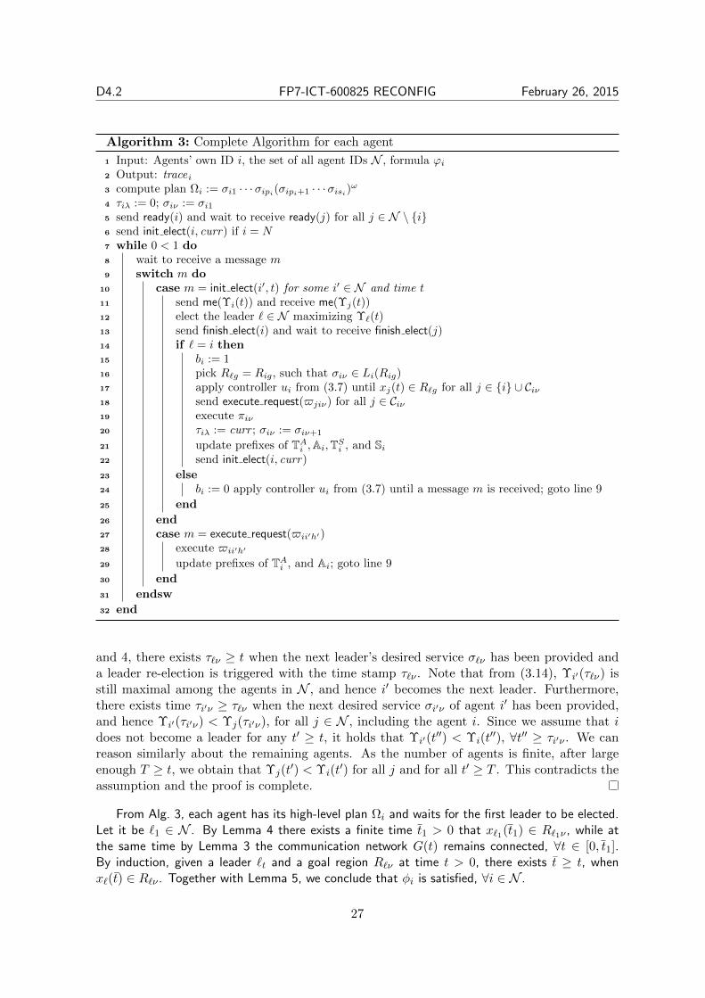
Algorithm 3: Complete Algorithm for each agent
1 Input: Agents’ own ID i, the set of all agent IDs N , formula ϕi2 Output: tracei3 compute plan Ωi := σi1 · · ·σipi(σipi+1 · · ·σisi)ω4 τiλ := 0; σiν := σi15 send ready(i) and wait to receive ready(j) for all j ∈ N \ i6 send init elect(i, curr) if i = N7 while 0 < 1 do8 wait to receive a message m9 switch m do
10 case m = init elect(i′, t) for some i′ ∈ N and time t11 send me(Υi(t)) and receive me(Υj(t))12 elect the leader ` ∈ N maximizing Υ`(t)13 send finish elect(i) and wait to receive finish elect(j)14 if ` = i then15 bi := 116 pick R`g = Rig, such that σiν ∈ Li(Rig)17 apply controller ui from (3.7) until xj(t) ∈ R`g for all j ∈ i ∪ Ciν18 send execute request($jiν) for all j ∈ Ciν19 execute πiν20 τiλ := curr ; σiν := σiν+1
21 update prefixes of TAi ,Ai,TSi , and Si22 send init elect(i, curr)
23 else24 bi := 0 apply controller ui from (3.7) until a message m is received; goto line 9
25 end
26 end27 case m = execute request($ii′h′)28 execute $ii′h′
29 update prefixes of TAi , and Ai; goto line 9
30 end
31 endsw
32 end
and 4, there exists τ`ν ≥ t when the next leader’s desired service σ`ν has been provided anda leader re-election is triggered with the time stamp τ`ν . Note that from (3.14), Υi′(τ`ν) isstill maximal among the agents in N , and hence i′ becomes the next leader. Furthermore,there exists time τi′ν ≥ τ`ν when the next desired service σi′ν of agent i′ has been provided,and hence Υi′(τi′ν) < Υj(τi′ν), for all j ∈ N , including the agent i. Since we assume that idoes not become a leader for any t′ ≥ t, it holds that Υi′(t
′′) < Υi(t′′), ∀t′′ ≥ τi′ν . We can
reason similarly about the remaining agents. As the number of agents is finite, after largeenough T ≥ t, we obtain that Υj(t
′) < Υi(t′) for all j and for all t′ ≥ T . This contradicts the
assumption and the proof is complete.
From Alg. 3, each agent has its high-level plan Ωi and waits for the first leader to be elected.Let it be `1 ∈ N . By Lemma 4 there exists a finite time t1 > 0 that x`1(t1) ∈ R`1ν , while atthe same time by Lemma 3 the communication network G(t) remains connected, ∀t ∈ [0, t1].By induction, given a leader `t and a goal region R`ν at time t > 0, there exists t ≥ t, whenx`(t) ∈ R`ν . Together with Lemma 5, we conclude that φi is satisfied, ∀i ∈ N .
27

D4.2 FP7-ICT-600825 RECONFIG February 26, 2015
Corollary 1. Algorithm 3 solves Problem 2.
3.5 Example
In the following case study, we present an example of a team of four autonomous robots withheterogeneous functionalities. All simulations are carried out on a desktop computer (3.06 GHzDuo CPU and 8GB of RAM).
3.5.1 System Description
Denote by the agents R1, R2, R3 and R4. They all satisfy the dynamics (3.1). They all havethe communication radius 1.5m, while ε is 0.1m. The workspace of size 4m × 4m is given inFigure 3.1, within which the regions of interest for R1 are R11, R12 (in red), for R2 are R21,R22 (in green), for R3 are R31, R32 (in blue) and for R4 are R41, R42 (in cyan). Besides themotion among these regions, each agent can provide various services as follows: agent R1 canload (lH , lA), carry and unload (uH , uA) a heavy object H or a light object A. Besides, it can helpR4 to assemble (hC) object C ; agent R2 is capable of helping the agent R1 to load the heavyobject H (hH), and to execute two tasks (t1, t2) without help; agent R3 is capable of takingsnapshots (s) when being present in its own or others’ goal regions; agent R4 can assemble (aC)object C under the help of agent R1.
3.5.2 Task Description
Each agent has been assigned a local complex task that requires collaboration: agent R1 has toperiodically load the heavy object H at region R11, unload it at region R12, load the light objectA at region R12, unload it at region R11. In LTL formula, it is specified as φ1 = GF
((lH ∧
hH ∧ r11) ∧ X(uH ∧ r12))∧ GF
((lA ∧ r12) ∧ (uA ∧ r11)
); Agent R2 has to service the simple
task t1 at region R21 and task t2 at region R22 in sequence, but it requires R2 to witness theexecution of task t2, by taking a snapshot at the moment of the execution. It is specified asφ2 = F
((t1 ∧ r21) ∧ F(t2 ∧ s ∧ r22)
); Agent R3 has to surveil over both of its goal regions (R31,
R32) and take snapshots there, which is φ3 = GF(s∧r31)∧GF(s∧r32); Agent R4 has to assembleobject C at its goal regions (R41, R42) infinitely often, which is φ4 = GF(aC ∧r41)∧GF(aC ∧r42).Note that φ1, φ3 and φ4 require collaboration tasks be performed infinitely often.
3.5.3 Simulation Results
Initially, the agents start evenly from the x-axis, i.e., (0, 0), (1.3, 0), (2.6, 0), (3.9, 0). By Def. 13,the initial edge set is E(0) = (1, 2), (2, 3), (3, 4), yielding a connected G(0). The system issimulated for 35s, of which the video demonstration can be viewed here [83]. In particular, Alg. 3is followed. Initially, agent R1 is chosen as the leader. As a result, controller (3.4) is applied forR1 as the leader and the rest as followers, while the next goal region of R1 is R11. As shown byLemma 4, all agents belong to R11 after t = 3.8s. After that agent R2 helps agent R1 to loadobject H. Then agent R2 is elected as the leader after collaboration is done, where R21 is chosenas the next goal region. At t = 6.1s, all agents converge to R21. Afterwards, the leader and goalregion is switched in the following order: R3 as leader to region R31 at t = 6.1s; R4 as leader toregion R41 at t = 8.1s; R4 as leader to region R42 at t = 10.6s; R2 as leader to region R22 att = 14.2s; R3 as leader to region R32 at t = 16.3s; R1 as leader to region R12 at t = 18.2s; R1
28

D4.2 FP7-ICT-600825 RECONFIG February 26, 2015
0.0 0.5 1.0 1.5 2.0 2.5 3.0 3.5 4.0y (m)
0.0
0.5
1.0
1.5
2.0
2.5
3.0
3.5
4.0
x (m
)
Robot 1Robot 2
Robot 3Robot 4
0 5 10 15 20 25 30 35Time (s)
0.0
0.2
0.4
0.6
0.8
1.0
1.2
1.4
Dis
tance
(m
)
d12d23d34
Figure 3.1. Left: the agents’ trajectory during time [0, 34.8s]; Right: the evolution of pair-wise distances‖x12‖, ‖x23‖, ‖x34‖, which all stay below the radius 1.5m as required by the connectivity constraints.
as leader to region R11 at t = 20.1s; R3 as leader to region R31 at t = 24.2s; R3 as leader toregion R32 at t = 25.7s; R4 as leader to region R41 at t = 28.1s. R4 as leader to region R42 att = 31.4s.
Figure 3.1 shows the trajectory of R1, R2, R3, R4 during time [0, 34.7s], in red, green,blue, cyan respectively. Furthermore, the pairwise distance for neighbours within E(0) is shownin Figure 3.1. It can be verified that they stay below the constrained radius 1.5m thus the agentsremain connected.
3.6 Summary
We present a distributed motion and task control framework for multi-agent systems under complexlocal LTL tasks and connectivity constraints. Our approach guarantees that all individual tasksare fulfilled, while at the same time connectivity constraints are satisfied.
29

Chapter 4
Multi-Agent LTL Plan Execution underImplicit Communication
4.1 Introduction
In this Chapter, we provide results on the problem controlling a two-agent system with local LTLspecifications. We are motivated by the scenario of two agents collaborating to carry an object ina leader-follower formation. We assume that the agents lack the ability to communicate explicitlyby exchanging messages. As a solution, we propose a control algorithm based on periodical leaderre-election that guarantees both agents’ local goal satisfaction under implicit communication. Anillustrative experiment of our results is included in Deliverable D5.4.
The chapter is organized as follows. In Sections 4.2 and 4.3 we provide the preliminaries andthe formulate the problem. In Section 4.4 the solution of the problem is analyzed and we concludein Section 4.5.
4.2 Preliminaries
Given a set S, we denote by 2S the set of all subsets of S. Given a finite sequence s1 . . . snof elements of S, we denote by (s1 . . . sn)ω the infinite sequence s1 . . . sns1 . . . sn . . . created byrepeating s1 . . . sn.
Definition 14 (LTL). An Linear Temporal Logic (LTL) formula φ over the set of servicesΠ is defined inductively as follows:
(i) every service π ∈ Π is a formula, and
(ii) if φ1 and φ2 are formulas, then φ1 ∨ φ2, ¬φ1, Xφ1, φ1 Uφ2, Fφ1, and Gφ1 are each aformula,
where ¬ (negation) and ∨ (disjunction) are standard Boolean connectives, and X (next), U(until), F (eventually), and G (always) are temporal operators.
The semantics of LTL are defined over infinite words over 2Π. Intuitively, an atomic propositionπ ∈ Π is satisfied on a word w = $1$2 . . . if it holds at its first position $1, i.e. if π ∈ $1.Formula Xφ holds true if φ is satisfied on the word suffix that begins in the next position $2,
30
D4.2 FP7-ICT-600825 RECONFIG February 26, 2015
whereas φ1 Uφ2 states that φ1 has to be true until φ2 becomes true. Finally, Fφ and Gφ aretrue if φ holds on w eventually, and always, respectively. For the full formal definition of the LTLsemantics see, e.g. [4].
4.3 Problem Formulation
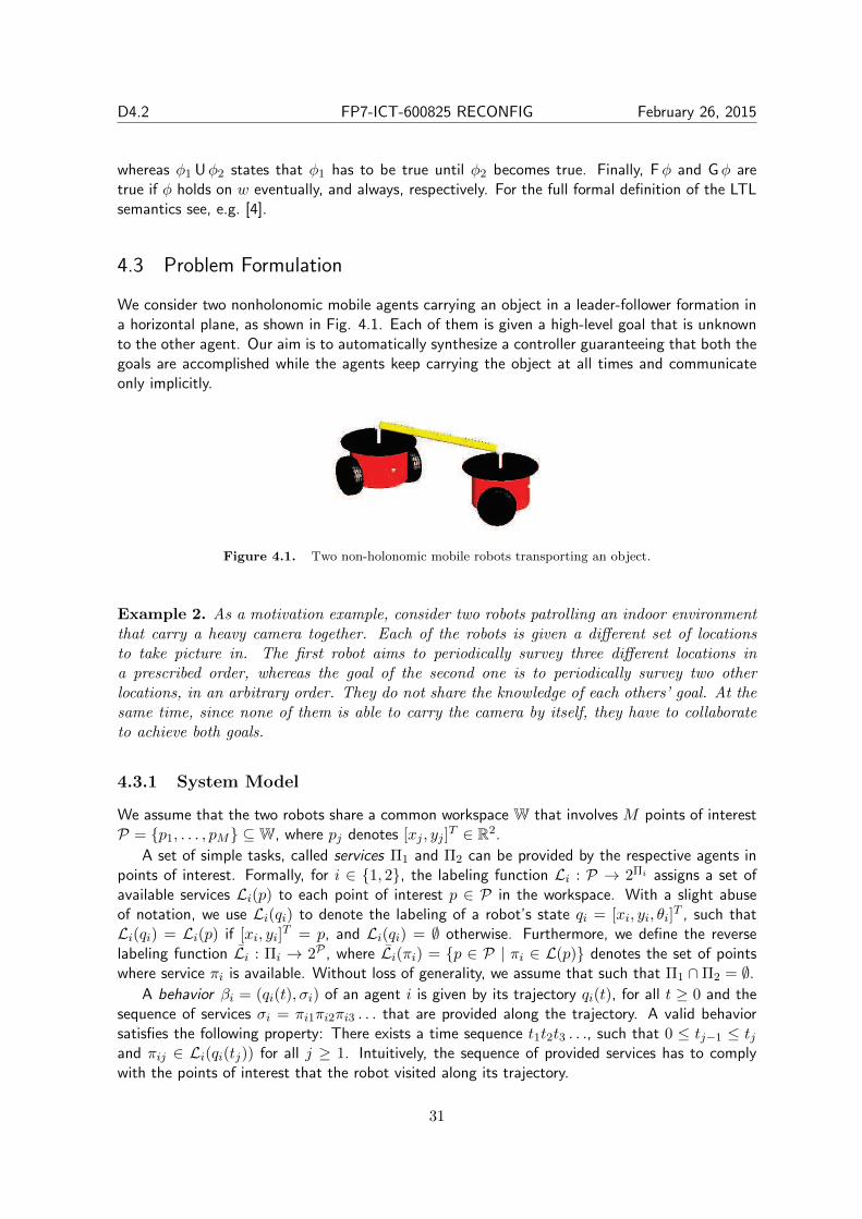
We consider two nonholonomic mobile agents carrying an object in a leader-follower formation ina horizontal plane, as shown in Fig. 4.1. Each of them is given a high-level goal that is unknownto the other agent. Our aim is to automatically synthesize a controller guaranteeing that both thegoals are accomplished while the agents keep carrying the object at all times and communicateonly implicitly.
Figure 4.1. Two non-holonomic mobile robots transporting an object.
Example 2. As a motivation example, consider two robots patrolling an indoor environmentthat carry a heavy camera together. Each of the robots is given a different set of locationsto take picture in. The first robot aims to periodically survey three different locations ina prescribed order, whereas the goal of the second one is to periodically survey two otherlocations, in an arbitrary order. They do not share the knowledge of each others’ goal. At thesame time, since none of them is able to carry the camera by itself, they have to collaborateto achieve both goals.
4.3.1 System Model
We assume that the two robots share a common workspace W that involves M points of interestP = p1, . . . , pM ⊆W, where pj denotes [xj , yj ]
T ∈ R2.
A set of simple tasks, called services Π1 and Π2 can be provided by the respective agents inpoints of interest. Formally, for i ∈ 1, 2, the labeling function Li : P → 2Πi assigns a set ofavailable services Li(p) to each point of interest p ∈ P in the workspace. With a slight abuseof notation, we use Li(qi) to denote the labeling of a robot’s state qi = [xi, yi, θi]
T , such thatLi(qi) = Li(p) if [xi, yi]
T = p, and Li(qi) = ∅ otherwise. Furthermore, we define the reverselabeling function Li : Πi → 2P , where Li(πi) = p ∈ P | πi ∈ L(p) denotes the set of pointswhere service πi is available. Without loss of generality, we assume that such that Π1 ∩Π2 = ∅.
A behavior βi = (qi(t), σi) of an agent i is given by its trajectory qi(t), for all t ≥ 0 and thesequence of services σi = πi1πi2πi3 . . . that are provided along the trajectory. A valid behaviorsatisfies the following property: There exists a time sequence t1t2t3 . . ., such that 0 ≤ tj−1 ≤ tjand πij ∈ Li(qi(tj)) for all j ≥ 1. Intuitively, the sequence of provided services has to complywith the points of interest that the robot visited along its trajectory.
31

D4.2 FP7-ICT-600825 RECONFIG February 26, 2015
4.3.2 Control Objective
The control objectives are given for each robot separately as an LTL formula φ1 and φ2 over Π1
and Π2, respectively. An LTL formula φi is satisfied if the behavior of the robot i is βi = (qi(t), σi)where σi is infinite and satisfies φi.
4.3.3 Problem Formulation
Problem 3. Given two nonholonomic mobile robots subject to leader-follower force/torquedynamics in a partitioned, labeled workspace, and two LTL formulas φ1, φ2 over their respec-tive service sets Π1, Π2, find behaviors β1 and β2 of the two robots that yield the satisfactionof both LTL formulas φ1 and φ2.
Example 1 (cont.): Recall the setup from Example 2. Let P = P1, . . . , P5 be the setof 5 mentioned points of interest. For i ∈ 1, 2, the set of services that can be provided isΠi = Pij = “Robot i visits Pj” | Pj ∈ P. The goal of the first robot is to survey P1, P4, P5,in this order, which can be represented as an LTL formula φ1 = G F (P11 ∧ X (P14 ∧ XP15))). Incontrast, the second robot is to survey P2 and P3, in an arbitrary order, which can be expressedas φ2 = G FP22 ∧ G FP23.
4.4 Problem Solution
4.4.1 Solution Overview
Our approach to solving Problem 3 consists of the following three steps that are described indetails later in this section.
Step A
For each agent, we generate a sequence of services that, if provided, guarantee the satisfaction ofthe respective formula. Using the reverse labeling functions L1 and L2, we find high-level plans,i.e. corresponding sequences of regions, called waypoints, where these services can be provided.Thus, we decompose the problem of planning under LTL goals into a sequence of reachabilitycontrol problems for each agent.
Step B
We set one (an arbitrary one) of the agents as the leader while the other one is the follower. Wepropose an implicit communication-based leader-follower control scheme that takes the leader tothe next waypoint on its high-level plan while respecting the given system model. In other words,the follower assists the leader without requesting any explicit feedback. The details are presentedin Deliverable D3.3.
Step C
When a waypoint is reached, the corresponding service is provided. The leader is then re-electedand a new reachability goal is set to the next waypoint on the plan. We introduce a systematicswitching protocol of the agents’ roles by which we ensure that both agents keep making progress
32

D4.2 FP7-ICT-600825 RECONFIG February 26, 2015
towards their respective LTL goals, i.e. that they both gradually visit waypoints on their high-level plans. The switching is executed solely with implicit communication as summarized inDeliverable D3.3.
4.4.2 High-Level Plan Generation
The first ingredient of our solution is the high-level plan, which can be generated using standardtechniques inspired by automata-based formal verification methodology. Namely, an LTL formulaφi is first translated into a Buchi automaton. Then, the automaton is viewed as a graph andanalyzed using graph search algorithms. Loosely speaking, an accepting run of the automatonprojects directly onto a sequence of services to be provided and hence onto a sequence of waypointsto be visited. Although the semantics of LTL is defined over infinite sequences of services, it canbe proven that there always exists a high-level plan that takes a form of an infinite repetition ofa finite service/waypoint sequence. More details on the technique are beyond the scope of thechapter and we refer the reader to related literature, e.g., [4].
To sum up, we have obtained a high-level plan for each robot i ∈ 1, 2 given as a sequence ofwaypoints and services: ςi = (pi1 . . . piN )ω, and σi = (πi1 . . . πiN )ω, where pij ∈ P, and πij ∈ Πi,for all j ∈ 1, . . . , N and some finite N ∈ N.
4.4.3 Leadership Switching based on Implicit Communication
An extra issue to be discussed herein is how to select the leader after a certain task has beenaccomplished (i.e., which one should be assigned the leadership). We propose to adopt a decen-tralized decision scheme according to which the agent with the shortest/closest task should claimthe leadership. However, relying only on a distance criterion is not truly “fair”, especially in caseswhere each agent’s tasks are collected in distant and disjoint areas. In this way, only one agentwould gain the leadership repeatedly, since the other’s goals are far away. Thus, we have to makea trade-off between time efficiency and “fairness” such that all individual goals of both agents aresuccessfully accomplished eventually. Therefore, a “racing” algorithm should be adopted after atask is fulfilled, based on which both agents will claim the leadership in a time interval that isproportional to the distance from their next task as well as to the number of consecutive timesthey have been leading the formation until then. Hence, the agent that has not been leadingmuch lately, with a relatively close task will ultimately be getting the leadership. In this way, weformulate for each agent the following “racing” criterion:
Ci = W1‖qi − qNextid‖+W2N
Ledi , i = 1, 2 (4.1)
where W1, W2 are positive weights, favoring either the efficiency or the “fairness” of the criterion,qi, q
Nextid
are the current and the next desired state according to the agents’ individual task
specifications and NLedi denotes the number of successive leaderships of each agent until now.
It should be noticed that in order to apply properly the aforementioned “racing” algorithm,after a task has been fulfilled, the agents have to be synchronized first. Nonetheless, explicitcommunication, which is the easiest way to achieve it, is not feasible in our work. Thus, thesynchronization should be accomplished via implicit communication through the physical inter-action of the agents. However, such implicit information should be acquired independently ofthe force/torque measurements that are employed by the follower’s scheme to cooperate with theleader (i.e., a force along the object and a torque around the vertical axis), since otherwise animplicit misunderstanding would occur. In this sense, we propose to use the measurement of the
33

D4.2 FP7-ICT-600825 RECONFIG February 26, 2015
force exerted at the follower’s side by a periodic rotation of the leader around itself. Such motionprimitive does not affect the follower’s motion, since it does not change the force/torque feedbackemployed in its control scheme.
Hence, the procedure of mechanical synchronization is given as follows:1. The current leader, after having accomplished its task, starts rotating periodically with a
predefined frequency Fsyn around itself for a certain prespecified time Tsyn.2. The follower measures the exerted force and detects the time instant at which the leader
stopped rotating by observing when the Maximum Likelihood frequency estimate index CML(ω)is maximized [50], for a given frequency ωsyn = 2πFsyn within a sample of N force measurementsin a moving window of Tsyn duration (i.e., fm[i], i = 0, . . . , N − 1), where:
CML (ω) =a22 (ω) I2 (ω)− 2a12 (ω) I (ω)Q (ω) + a11 (ω)Q2 (ω)
a11 (ω) a22 (ω)− a212 (ω)
with I (ω) =∑N−1
i=0 fm [i] cos (iω), Q (ω) =∑N−1
i=0 fm [i] sin (iω), a11 (ω) =∑N−1
i=0 cos2 (iω),
a12 (ω) =∑N−1
i=0 sin (iω) cos (iω) and a22 (ω) =∑N−1
i=0 sin2 (iω).
Remark 3. Notice that the only information that should be agreed by the agents consists in thesynchronization parameters Fsyn and Tsyn, which however can be easily done at the beginningbefore starting the execution of their plans. Moreover, the computation of the ML frequencyestimator CML(ωsyn) involves very few and simple calculations, which can be implementedon-line without introducing further delays.
4.4.4 Algorithm Analysis
Theorem 1. By following the three steps A, B, C of the solution, we achieve behaviors ofrobots 1 and 2 are both infinite and satisfy φ1 and φ2, respectively.
Proof. Thanks to the correctness of well-establish algorithms for finding high-level plans de-scribed in step A, it is enough to prove that steps B and C ensure that the plans are executed.In step B, we have proven that given that the desired position [xd, yd]
T of the leader is reachedin finite time. Furthermore, Eq. 4.1 in step C is proposed in such a way that for all timeinstants t, when C1 < C2, there exists t′ > t when C2 < C1 and vice versa, if C2 < C1 at t,then C1 < C2 at some t′. Each agent hence becomes a leader infinitely often and remains theleader till it reaches its next desired position [xd, yd]
T , i.e. the next waypoint of the high-levelplan. Altogether, we conclude that both agents visit the prescribed waypoints infinitely manytimes and hence their behaviors satisfy φ1 and φ2.
4.5 Summary
We have provided a decentralized solution for the problem of controlling two collaborating robotswith individual LTL specifications in the absence of explicit inter-robot communication. Oursolution is based on a leader-follower scheme, with an implicit communication type re-electionstrategy and guarantees the fulfillment of both individual goal specifications.
34

Chapter 5
Multi-agent Task Coordination and FaultTolerance Analysis
In the first part of this chapter we propose a bottom-up motion and task coordination scheme formulti-agent systems under dependent local tasks. We assume that each agent is assigned locallya task by means of LTL formulas that specify both motion and action requirements. Inter-agentdependency is introduced by collaborative actions whose execution requires the collaboration ofmultiple agents. We propose a distributed solution based on an off-line initial plan synthesis, anon-line request-reply messages exchange and a real-time plan adaptation algorithm. The solutionis scalable and resilient to agent failures as the dependency is formed and removed dynamicallybased on the plan execution status and agent capabilities, instead of pre-assigned agent identities.In the second part of the chapter, we exploit the paradigm of a single robot system controlledby a Behavior Tree (BT) and demonstrate how multi-robot teams offer possibilities of improvedperformance and fault tolerance, compared to single robot solutions. In particular, we show howthey can be improved in a single robot BT, by adding more robots to the team and extending theBT into a multi-robot BT.
The chapter is organized as follows. In Sections 5.1 and 5.2 we provide the preliminaries andthe problem formulation for multi-agent task coordination. We proceed with the description ofthe initial plan synthesis in Section 5.3 and provide the distributed online coordination schemein Section 5.4. The overall structure is discussed in Sections 5.5 and a case study is provided inSection 5.6. We proceed with background on BTs in Section 5.7 and formulate the decentralizedBT controller problem in Section 5.8. In Section 5.9 we provide the corresponding solution anddiscuss a motivating example in Section 5.10. We summarize the chapter in Section 5.11.
5.1 Preliminaries
5.1.1 Co-safe LTL and Buchi Automaton
Atomic propositions are Boolean variables that can be either true or false. The ingredients of anLTL formula are a set of atomic propositions AP and several boolean and temporal operators,which are specified according to the following syntax [4]: ϕ ::= True | p | ϕ1 ∧ ϕ2 | ¬ϕ | ©ϕ | ϕ1Uϕ2, where p ∈ AP and © (next), U (until). For brevity, we omit the derivations of otheruseful operators like (always), ♦ (eventually), ⇒ (implication) and the semantics of LTL. Werefer the readers to Chapter 5 of [4]. One particular class of LTL formulas we consider in this
35
D4.2 FP7-ICT-600825 RECONFIG February 26, 2015
part of the chapter are syntactically co-safe formulas [62]. They only contain the ©, U and ♦operators and are written in positive normal form. Informally, any trace satisfying such a formulahas a finite good prefix. A finite good prefix is a finite prefix such that all its trace extensionssatisfy the formula.
There exists a Nondeterministic Buchi automaton (NBA) Aϕ corresponding to ϕ [4], which isdefined as Aϕ = (Q, 2AP , δ, Q0, F), where Q is a set of states; 2AP is the set of all alphabets;δ ⊆ Q× 2AP ×Q is a transition relation; Q0,F ⊆ Q are the initial and accepting states. Thereare fast translation tools [31] to obtain Aϕ given ϕ.
5.2 Problem Formulation
We considerK autonomous agents with heterogeneous capabilities within a fully-known workspace.Each agent with the identity k ∈ K = 1, 2, · · · ,K is capable of navigating within the workspaceand performing various actions.
5.2.1 Motion Abstraction
The workspace consists ofN partitions as the regions of interest, denoted by Π = π1, π2, · · · , πN.We assume that these symbols are assigned in priori and known by all agents. There are differentcell decomposition techniques available, depending on the agent dynamics and the associatedcontrol approaches, see [7], [22], [67]. Besides, there is a set of atomic propositions describingthe properties of the workspace, denoted by Ψk
M. Similar to [35], agent k’s motion within theworkspace is modeled as a finite transition system (FTS):
Mk , (Π, −→kM, Πk
M,0, ΨkM, L
kM, T
kM), (5.1)
where −→kM⊆ Π × Π is the transition relation; Πk
M,0 ∈ Π is the initial region agent k starts
from; LkM : Π → 2ΨkM is the labeling function, indicating the properties held by each region;
T kM :−→kM→ R+ estimates the time each transition takes. Note thatMk might be different due
to heterogeneity. The workspace model from Sec. 5.6 is shown in Fig. 5.1.Moreover, each agent k has a set of neighboring agents, denoted by Kk ⊆ K. We assume
that agent k can exchange messages directly with any agent belonging to Kk.
5.2.2 Action Model
Besides the motion ability, agent k is capable of performing a set of actions denoted by Σk ,Σkl ∪ Σk
c ∪ Σkh, where
• Σkl is a set of local actions, which can be done by agent k itself;
• Σkc is a set of collaborative actions, which can be done by agent k but requires collaborations
from other agents;
• Σkh is a set of assisting actions, which agent k offers to other agents to accomplish their
collaborative actions.
In other words, Σkl and Σk
c contain active actions that can be initiated by agent k, denoted byΣka = Σk
l ∪ Σkc , while Σk
h contains passive actions to assist other agents. By default, σ0 = None ∈Σkl means that none of the actions is performed. Moreover, denote by Σ∼kh the set of external
36

D4.2 FP7-ICT-600825 RECONFIG February 26, 2015
0.0 0.5 1.0 1.5 2.0 2.5 3.0 3.5 4.0y (m)
0.0
0.5
1.0
1.5
2.0
2.5
3.0
3.5
4.0
x (m
)
r4 B
r5 C r6
r7 B
r0
r1 A r2 E
r3 F
r8 M
0.0 0.5 1.0 1.5 2.0 2.5 3.0 3.5 4.0y (m)
0.0
0.5
1.0
1.5
2.0
2.5
3.0
3.5
4.0
x (m
)
r4
r5 r6
r7
r0
r1 r2
r3
r8
Robot 1Robot 2
Robot 3Robot 4
Robot 5Robot 6
Figure 5.1. Left: the regions are in gray and labeled by objects of interest inside; Right: the final trajectoriesof all agents after accomplishing their local tasks in Sec. 5.6.3.
assisting actions agent k depends on, which can only be provided by some of its neighbors in Kk,i.e., Σ∼kh ⊆ ∪i∈KkΣi
h. Table 5.1 shows the action sets of the agents that will be simulated inSec. 5.6.
The action model of agent k is modeled by a six-tuple:
Ak , (Σk, ΨkΣ, L
kΣ, Cond
k, Durak, Depdk), (5.2)
where Σk is the set of actions defined earlier; ΨkΣ is a set of atomic propositions related to the
agent’s active actions; LkΣ : Σk → 2ΨkΣ is the labeling function. LkΣ(σh) = ∅, ∀σh ∈ Σk
h and
LkΣ(σa) ⊆ ΨkΣ, ∀σa ∈ Σk
a; Condk : Σk×2ΨkM → True/False indicates the set of region properties
that have to be fulfilled in order to perform an action; Durak : Σk → R+ is the time duration ofeach action. Durak(σ0) = T0 > 0 is a design parameter; Depdk : Σk → 2Σ∼k
h is the dependencefunction. Depdk(σs) = ∅, ∀σs ∈ Σk
l ∪ Σkh and Depdk(σc) ⊆ Σ∼kh , ∀σc ∈ Σk
c . Namely eachcollaborative action depends on a set of assisting actions from its neighbors. This is useful fordefining complex collaborations involving multiple agents.
Remark 4. Compared with defining dependency directly on agent identities, our action modelallows more system flexibility since the agent identities need not be known a priori and newor existing agents can be added or removed.
Definition 15. A local or assisting action σs ∈ Σkl ∪Σk
h is said to be done at region πi ∈ Π iftwo condition holds: (i) Condk(σs, L
kM(πi)) = True; (ii) σs is activated for period Durak(σs).
For a collaborative action σc ∈ Σkc , another condition is needed: (iii) all assisting actions in
Depdk(σc) are done by other agents at the same region πi.
Remark 5. Different from [35], the action model by (5.2) can model both local and collabo-rative actions.
37

D4.2 FP7-ICT-600825 RECONFIG February 26, 2015
Agent Σkl Σk
c Σkh Σ∼kh
R1 lA, uA lB, uB ∅ hBR2 s ∅ hB, hC1 , hF ∅R3 ∅ oM hC2 , hF hMR4 s aC hM , hF hC1 , hC2
R5 mD ∅ hB, hC1 , hC2 ∅R6 oE cF hB, hM hF
Table 5.1. Action sets of the agents described in Sec. 5.6.
5.2.3 Complete Agent Model
A complete agent model, denoted by Gk, refers to the finite transition system that models bothits motion and actions.
Definition 16. Given Mk and Ak, agent k’s complete model can be constructed as follows:
Gk = (ΠkG , −→k
G , ΠkG,0, Ψk
G , LkG , T
kG ), (5.3)
where ΠkG = Π × Σk. πG,i = 〈πj , σn〉 ∈ Πk
G, ∀πj ∈ Π, ∀σn ∈ Σk; −→kG⊆ Πk
G × ΠkG.(
〈πi, σm〉, 〈πj , σn〉)∈−→k
G if (i) σn = σm = σ0, πi −→kM πj; or (ii) σm = σ0, σn 6= σ0 and
πi = πj, Condk(σn, L
kM(πi)) = True; Πk
G,0 = ΠkM,0 × σ0 is the initial state; Ψk
G = ΨkM ∪Ψk
Σ;
LkG : ΠkG → 2Ψk
. LkG(〈πi, σm〉) = LkM(πi) ∪ LkΣ(σm); T kG :−→kG→ R+. For case (i) above,
T kG (〈πi, σm〉, 〈πj , σn〉) = T kM(πi, πj); for case (ii), T kG (〈πi, σm〉, 〈πj , σn〉) = Durak(σn).
Note that when defining −→kG above, the condition of performing an action is verified over
the properties of each region. Thus Gk is a standard FTS [4]. Its finite path is denoted by τk =πG,0πG,1 · · ·πG,N , where πG,i ∈ Πk
G , πG,0 ∈ ΠkG,0 and (πG,i, πG,i+1) ∈−→k
G , ∀i = 0, · · · , N − 1. Its
trace is trace(τk) = LkG(πG,0)LkG(πG,1) · · ·LkG(πG,N ).
5.2.4 Task Specification
The local task of agent k, denoted by ϕk, is given as a co-safe LTL formula over the set ofatomic propositions Ψk
G from (5.3). Thus ϕk can contain requirements on agent’s motion, localand collaborative actions. As mentioned earlier, a co-safe LTL formula can be fulfilled by a finiteprefix over Ψk
G . In particular, given a finite path τk of Gk, then τk fulfils ϕk if trace(τk) |= ϕk
where the satisfaction relation is defined in Sec. 5.1.1. One special case is that when ϕk , True,agent k does not have a local task and serves as an assisting agent.
Definition 17. The tasks ϕk, k ∈ K are called mutually feasible for the team if the mutualtask ϕ1 ∧ ϕ2 ∧ · · ·ϕK is feasible for the composed system G1 × G2 × · · · GK .
For detailed definition of the mutual feasibility and the composed system, we refer the readersto Sect. IV.A of [37].
5.2.5 Problem Formulation
Problem 4. Given Gk and the locally-assigned task ϕk, assume ϕk, k ∈ K are mutuallyfeasible by Def. 17, then design a distributed control and coordination scheme such that ϕk isfulfilled for all k ∈ K.
38
D4.2 FP7-ICT-600825 RECONFIG February 26, 2015
5.3 Off-line Initial Plan Synthesis
In this section, we describe how to synthesize an initial motion and action plan for each agent,which happens off-line and serves as a starting point for the real-time coordination and adaptationscheme in Sect. 5.4.
5.3.1 Plan as Motion and Action Sequence
We intend to find a finite path of Gk whose trace satisfies the co-safe formula ϕk as describedin Sec. 5.2.4. We rely on the automaton-based model-checking approach (see Alg. 11 in [4]) bychecking the emptiness of the product automaton. Let Aϕk be the NBA associated with ϕk from
Sec. 5.1.1. The product automaton Akp is defined as follows:
Akp = Gk ⊗Aϕk = (Qkp, δkp , Q
kp,0, Fkp , W k
p ), (5.4)
where Qkp = ΠkG ×Qk, qp = 〈πG,j , qn〉 ∈ Qkp, ∀πG,j ∈ Πk
G , ∀qn ∈ Qk; (〈πG,i, qm〉, 〈πG,j , qn〉) ∈ δkpif πG,i −→k
G πG,j and (qm, LkG(πG,i), qn) ∈ δk ; Qkp,0 = Πk
G,0 × Qk0 is the set of initial states;
Fkp = ΠkG × Fk is the set of accepting states; W k
p : Qkp ×Qkp → R+. W kp (〈πG,i, qm〉, 〈πG,j , qn〉)
= T kG (πG,i, πG,j), where 〈πG,j , qn〉 ∈ δkp(〈πG,i, qm〉).
There exists a finite path of Gk satisfying ϕk if and only if Akp has a finite path from aninitial state to an accepting state, and this accepting state is contained in a cyclic path. Thenthis path could be projected back to Gk as a finite path, the trace of which should satisfy ϕk
automatically [4]. Let Rkp = qkp,0qkp,1 · · · qkp,N be a finite path of Akp, where qkp,0 ∈ Qkp,0, qkp,N ∈ Fkp ,
qkp,i ∈ Qkp and (qkp,i, qkp,i+1) ∈ δkp , ∀i = 0, · · · , N − 1. The cost of Rkp is defined by
Cost(Rkp , Akp) =
N−1∑i=0
W kp (qkp,i, q
kp,i+1), (5.5)
which is the summed weights along Rkp . The ith element is given by Rkp [i] = qkp,i and the segment
from the ith to the jth element is Rkp [i : j] = qkp,iqkp,i+1 · · · qkp,j , where i ≤ j ≤ N .
Problem 5. Find a finite path Rkp of Akp with the above structure that minimizes the totalcost by (5.5).
Denote by Rkp,init the solution. Algorithm 1 in [35] solves the above problem, which is omittedhere due to limited space. It utilizes Dijkstra’s algorithm [64] for computing the shortest pathfrom any initial state in Qkp,0 to every reachable accepting state in Fkp and checks if there is cycle
back to qp,N . The worst-case complexity is O(|δkp | · log |Qkp| · |Qkp,0|). By projecting Rkp,init onto
ΠkG , it gives the initial motion and action plan τkG,init = Rkp,init|Πk
Gthat fulfils ϕk.
Remark 6. Different from [22] and [37], the initial plans are synthesized locally by each agentinstead of by a central unit or within a cluster.
τkG,init is executed by activating the motion or actions in sequence. However note that τkG,initmay contain several collaborative actions from Σk
c to satisfy ϕk. Thus the successful executionof τkG,init depends on other agents’ collaboration, which however is not guaranteed since τkG,init issynthesized off-line and locally by agent k. We resolve this problem by a real-time coordinationand adaptation scheme in Sec. 5.4.
39

D4.2 FP7-ICT-600825 RECONFIG February 26, 2015
Algorithm 4: Plan in horizon and request, Request()
Input: τkG,init, πkG,t, H
k
Output: τkG,H , Requestk
1 τkG,init[i] = πkG,t, s = 0, Tm = 0, Requestk = ∅;2 while T < Hk and i+ s ≤ |τkG,init| do
3 s = s+ 1;
4 Tm = Tm + T kG
(τkG, init[i], τ
kG,init[i+ s]
);
5 〈πi, σm〉 = τkG,init[i+ s];
6 if Requestk = ∅ and σm ∈ Σkc then
7 forall the σd ∈ Depdk(σm) do
8 add (σd, πi, Tm) to Requestk;9 end
10 end
11 end
12 j = i+ s, τkG,H = τkG,init[i : j];
13 return τkG,H , Requestk
5.4 Distributed Collaborative Task Coordination
As mentioned earlier, there is no guarantee that the initial plan τkG,init can be executed successfully ifit contains collaborative actions. In this section, we propose a distributed and on-line coordinationscheme which involves four major parts: (i) a request and reply exchange protocol driven bycollaborative actions in a finite horizon; (ii) an optimization and confirmation mechanism, bysolving a mixed integer program based on the replies; (iii) a real-time plan adaptation algorithmgiven the confirmation; (iv) an agent failure detection and recovery scheme along with the planexecution.
5.4.1 Planned Motion and Actions in Horizon
Denote by πkG,t ∈ ΠkG the state of agent k at time t. After the system starts, assume πkG,t is the
ith element in τkG,init, namely, πkG,t = τkG,init[i]. Each agent k ∈ K is given a bounded planning
horizon 0 < Hk <∞, which is the time ahead agent k checks its plan [101]. Then the sequenceof states agent k is expected to reach within the time Hk, denoted by τkG,H , is the segment
τkG,H = τkG,init[i : j], where the index j ≥ i is the solution to the problem below:
min j
s.t.
j∑s=i
T kG
(τkG, init[s], τ
kG,init[s+ 1]
)≥ Hk.
(5.6)
It can be solved by iterating through the sequence of τkG,init and computing the accumulated cost,
which is then compared with Hk. If (5.6) does not have a solution, it means Hk is larger thanthe total cost of the rest of the plan τkG,init[i : ], then j = |τkG,init|. The main reason of introducing
40

D4.2 FP7-ICT-600825 RECONFIG February 26, 2015
Algorithm 5: Reply to request by agent g, Reply()
Input: Requestkg , Rgp,−, Agp, T
g
Output: Replygk, P1 forall the (σd, πi, Tm) ∈ Requestkg do
2 if Tg
is 0 then
3(Rgp,+, b
gd, t
gd
)= EvalReq(Rgp,−, (πi, σd, Tm), Agp);
4 if bgd is True then
5 P (σd) = Rgp,+;
6 add (σd, bgd, t
gd) to Replygk;
7 end
8 end9 add (σd, False, 0) to Replygk
10 end
11 Return Replygk, P
the time horizon is to avoid coordinating on collaborative actions that will be done within a longtime from now. The above arguments are summarized in Lines 1-5, 9-10 of Alg. 4.
5.4.2 Request to Neighbours
Given τkG,H as the motion and actions in horizon, agent k needs to check whether it needs others’
collaboration within τkG,H . This is done by verifying whether a collaborative action needs to be
performed to reach the states in τkG,H . More specifically, for the first state 〈πi, σm〉 ∈ τkG,Hsatisfying σm ∈ Σk
c , agent k needs to broadcast a request to all agents within its communicationnetwork Kk regarding this action. This request message has the following format:
Requestk = (σd, πi, Tm), ∀σd ∈ Depdk(σm), (5.7)
where Depdk(σm) is the set of external assisting actions that σm depends on by (5.2); πi ∈ Π is theregion where σm will be performed; Tm ≥ 0 is the predicted time when σm will be performed from
now. Assume that 〈πi, σm〉 is the lth element of τkG,H . Then Tm =∑l
s=1 TkG
(τkG,H [s], τkG,H [s+ 1]
),
see Lines 4-9 of Alg. 4.Each element (σd, πi, Tm) ∈ Requestk contains the message that “agent k is requesting the
assisting action σd at region πi in time Tm from now”. The request message from agent k to eachagent g ∈ Kk, denoted by Requestkg , is the same as Requestk, i.e., Requestkg = Requestk, ∀g ∈Kk.
Remark 7. Note that the request message is sent only for the first collaborative action inτkG,H within the time horizon Hk (see Line 6 of Alg. 4). The reason is that the outcome ofthe first collaborative action would greatly affect the estimated execution time for the secondcollaborative action in τkG,H . More details can be found in Sec. 5.4.4.
5.4.3 Request Evaluation and Reply
Upon receiving the request, agent g ∈ Kk needs to evaluate this request in terms of feasibilityand cost, in order to reply to agent k. Specifically, the reply message from agent g to agent k
41
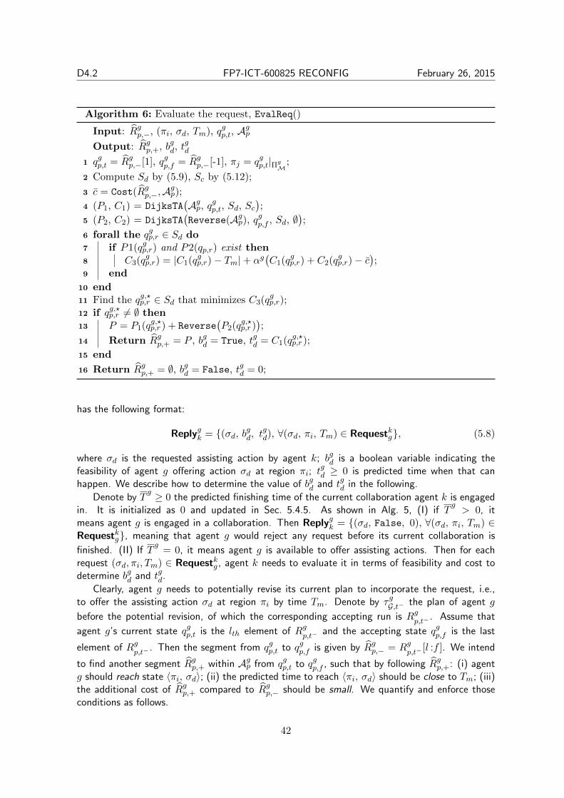
D4.2 FP7-ICT-600825 RECONFIG February 26, 2015
Algorithm 6: Evaluate the request, EvalReq()
Input: Rgp,−, (πi, σd, Tm), qgp,t, Agp
Output: Rgp,+, bgd, tgd
1 qgp,t = Rgp,−[1], qgp,f = Rgp,−[-1], πj = qgp,t|ΠgM
;
2 Compute Sd by (5.9), Sc by (5.12);
3 c = Cost(Rgp,−,Agp);
4 (P1, C1) = DijksTA(Agp, qgp,t, Sd, Sc
);
5 (P2, C2) = DijksTA(Reverse(Agp), qgp,f , Sd, ∅
);
6 forall the qgp,r ∈ Sd do7 if P1(qgp,r) and P2(qp,r) exist then8 C3(qgp,r) = |C1(qgp,r)− Tm|+ αg
(C1(qgp,r) + C2(qgp,r)− c
);
9 end
10 end11 Find the qg,?p,r ∈ Sd that minimizes C3(qgp,r);12 if qg,?p,r 6= ∅ then13 P = P1(qg,?p,r ) + Reverse
(P2(qg,?p,r )
);
14 Return Rgp,+ = P , bgd = True, tgd = C1(qg,?p,r );
15 end
16 Return Rgp,+ = ∅, bgd = False, tgd = 0;
has the following format:
Replygk = (σd, bgd, tgd), ∀(σd, πi, Tm) ∈ Requestkg, (5.8)
where σd is the requested assisting action by agent k; bgd is a boolean variable indicating thefeasibility of agent g offering action σd at region πi; t
gd ≥ 0 is predicted time when that can
happen. We describe how to determine the value of bgd and tgd in the following.
Denote by Tg ≥ 0 the predicted finishing time of the current collaboration agent k is engaged
in. It is initialized as 0 and updated in Sec. 5.4.5. As shown in Alg. 5, (I) if Tg> 0, it
means agent g is engaged in a collaboration. Then Replygk = (σd, False, 0), ∀(σd, πi, Tm) ∈Requestkg, meaning that agent g would reject any request before its current collaboration is
finished. (II) If Tg
= 0, it means agent g is available to offer assisting actions. Then for eachrequest (σd, πi, Tm) ∈ Requestkg , agent k needs to evaluate it in terms of feasibility and cost todetermine bgd and tgd.
Clearly, agent g needs to potentially revise its current plan to incorporate the request, i.e.,to offer the assisting action σd at region πi by time Tm. Denote by τ gG,t− the plan of agent g
before the potential revision, of which the corresponding accepting run is Rgp,t− . Assume that
agent g’s current state qgp,t is the lth element of Rgp,t− and the accepting state qgp,f is the last
element of Rgp,t− . Then the segment from qgp,t to qgp,f is given by Rgp,− = Rg
p,t− [l :f ]. We intend
to find another segment Rgp,+ within Agp from qgp,t to qgp,f , such that by following Rgp,+: (i) agentg should reach state 〈πi, σd〉; (ii) the predicted time to reach 〈πi, σd〉 should be close to Tm; (iii)the additional cost of Rgp,+ compared to Rgp,− should be small. We quantify and enforce thoseconditions as follows.
42

D4.2 FP7-ICT-600825 RECONFIG February 26, 2015
Firstly, the set of product states in Agp corresponding to 〈πi, σd〉 is given by
Sd = qp ∈ Qgp | qp|ΠgG
= 〈πi, σd〉. (5.9)
Let Rgp,+ have the following structure:
Rgp,+ = qgp,t · · · qgp,r · · · qgp,f , (5.10)
where qgp,r ∈ Sd, meaning that it passes through at least one state within Sd. Thus the corre-sponding plan would contain 〈πi, σd〉, which fulfils the condition (i) above. Regarding conditions(ii) and (iii), we define the balanced cost of Rgp,+:
BalCost(Rgp,+, Tm, Akp)
= |r−t∑s=1
W gp
(Rgp,+[s], Rgp,+[s+ 1]
)− Tm|
+ αg(Cost(Rgp,+, Akp)− Cost(Rgp,−, Akp)
),
(5.11)
where the first part stands for the time gap between the requested time Tm by agent k and theactual time based on Rgp,+ (for condition (ii)); the second term is the additional cost of Rgp,+,
compared to Rgp,− (for condition (iii)); αg > 0 is a design parameter as the relative weighting.
Problem 6. Given Rgp,−, Sd and Agp, find the path segement Rgp,+ that minimizes (5.11).
Alg. 6 solves the above problem by the bidirectional Dijkstra algorithm [77]. It utilizes thefunction DijksTA(·) that computes shortest paths in a weighted graph from the single sourcestate to every state in the set of target states, while at the same time avoiding a set of states. Itis a simple extension of the classic Dijkstra shortest path algorithm [64].
In Line 4, DijksTA(Agp, qgp,t, Sd, Sc) determines the shortest path (saved in P1) from qgp,t toevery state in Sd while avoiding any state belonging to Sc and the associated costs (saved in C1),where Sc is the set of all product states associated with a collaborative or assisting action:
Sc = qp ∈ Qgp | qp|ΠgG
= 〈πgG , σn〉, σn ∈ Σgc ∪ Σg
h. (5.12)
In Line 5, DijksTA(Reverse(Agp), qgp,f , Sd, ∅) is called to determined the shortest path (saved
in P2) from qgp,f to every state in Sd within the reversed Agp and the associated distances (saved in
C2); Reverse(Agp) is the directed graph obtained by inverting the direction of all edges in G(Agp)while keeping the weights unchanged, where G(Agp) is the directed graph associated with Agp [4].
In Lines 7-8, for each state qgp,r ∈ Sd, the balanced cost of the corresponding Rgp,+ by (5.11)
is computed. The one that yields the minimal cost is denoted by qg,?p,r . At last, Rgp,+ is formedby concatenating the shortest path from qgp,t to qg,?p,r and the reversed shortest path from qgp,f to
qg,?p,r . Last but not least, if qg,?p,r returns empty, it means that agent k could not offer the requestedcollaboration thus bgd = False and tgd = 0 as in Line 13. The complexity of function DijksTA(·)over Agp is O(|δgp | · log |Qgp|). Reversing Agp has the complexity linear to O(|δgp |).
Remark 8. Note that Rgp,+ is the potentially-revised run, meaning that agent g does not
change its current plan now but saves them in P (see Line 5 of Alg. 5) and waits for theconfirmation from agent k as discussed in Sec. 5.4.5.
43

D4.2 FP7-ICT-600825 RECONFIG February 26, 2015
Request R1, (hB, r4, 11) R4, (hC1 , r5, 14) R4, (hC2 , r5, 14)
R1 −− (hC1 , F, 0) (hC2 , F, 0)
R2 (hB, T, 13.1) (hC1 , T, 14.6) (hC2 , F, 0)
R3 (hB, F, 0) (hC1 , F, 0) (hC2 , T, 16.2)
R4 (hB, F, 0) −− −−R5 (hB, T, 15.7) (hC1 , T, 15.4) (hC2 , T, 15.4)
R6 (hB, T, 18.2) (hC1 , F, 0) (hC2 , F, 0)
Table 5.2. Request and reply messages exchanged for collaborative actions oM and aC in Sec. 5.6.
It is worth mentioning that in case agent k receives requests from multiple agents, it needs toreply to one agent first and wait for the confirmation before it replies to the next agent. Table 5.2shows the request and reply messages regarding two collaborative actions in Sec. 5.6.
Lemma 6. Given Rgp,+, bgd, tgd from Alg. 6, if bgd = True, action σd can be done at time tgd by
agent g following Rgp,+.
Proof. Since the first segment of Rgp,+ from qp,t to qg,?p,r is derived by DijksTA(·) in Line 5 ofAlg. 6, it does not contain any collaborative or assisting actions except σd. Thus it can beaccomplished by agent g itself with only motions and local actions, of which the predicatedtime is tgd.
5.4.4 Confirmation
Based on the replies from g ∈ Kk, agent k needs to acknowledge them by sending back confir-mation messages:
Confirmkg = (σd, cgd, fm),∀σd ∈ Depdk(σm), (5.13)
where σd is the requested assisting action; cgd is a boolean variable, indicating whether agent g isconfirmed to provide σd; fm is the updated time to finish action σm.
The choices of cgd, g ∈ Kk should satisfy two constraints: (i) exactly one agent in Kkt can
be the confirmed collaborator for each action σd ∈ Depdk(σm); (ii) each agent in Kk can beconfirmed for at most one action in Depdk(σm). Meanwhile, the finishing time fm should be asearly as possible.
Let |Kk| = N1 and |Depdk(σm)| = N2. Without loss of generality, denote by Kk =1, · · · , N1 and Depdk(σm) = σ1, · · · , σN2. The problem of finding cgd and fm can bereadily formulated as an integer programming problem [100]:
min fm
s.t. fm = maxdcgd · tgd, Tm
N2∑d=1
bgd · cgd ≤ 1, ∀g ∈ 1, · · · , N1,
N1∑g=1
bgd · cgd = 1, ∀d ∈ 1, · · · , N2,
(5.14)
where (σd, bgd, t
gd) ∈ Replygk from (5.8). Any stand-alone integer programming solver can be used
to obtain cgd and fm once (5.14) is formulated, e.g., “Gurobi” and “CVXOPT”.
44
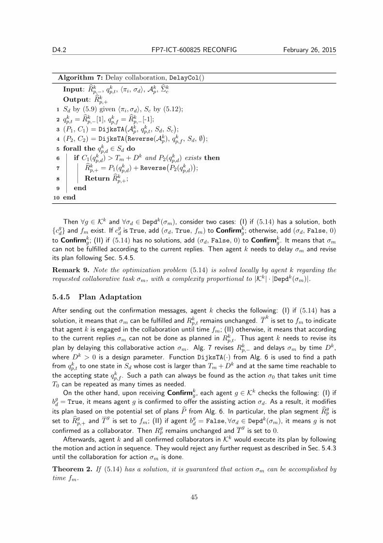
D4.2 FP7-ICT-600825 RECONFIG February 26, 2015
Algorithm 7: Delay collaboration, DelayCol()
Input: Rkp,−, qkp,t, 〈πi, σd〉, Akp, Σkc
Output: Rkp,+1 Sd by (5.9) given 〈πi, σd〉, Sc by (5.12);
2 qkp,t = Rkp,−[1], qkp,f = Rkp,−[-1];
3 (P1, C1) = DijksTA(Akp, qkp,t, Sd, Sc
);
4 (P2, C2) = DijksTA(Reverse(Akp), qkp,f , Sd, ∅
);
5 forall the qkp,d ∈ Sd do
6 if C1(qkp,d) > Tm +Dk and P2(qkp,d) exists then
7 Rkp,+ = P1(qkp,d) + Reverse(P2(qkp,d)
);
8 Return Rkp,+;
9 end
10 end
Then ∀g ∈ Kk and ∀σd ∈ Depdk(σm), consider two cases: (I) if (5.14) has a solution, bothcgd and fm exist. If cgd is True, add (σd, True, fm) to Confirmk
g ; otherwise, add (σd, False, 0)
to Confirmkg ; (II) if (5.14) has no solutions, add (σd, False, 0) to Confirmk
g . It means that σmcan not be fulfilled according to the current replies. Then agent k needs to delay σm and reviseits plan following Sec. 5.4.5.
Remark 9. Note the optimization problem (5.14) is solved locally by agent k regarding therequested collaborative task σm, with a complexity proportional to |Kk| · |Depdk(σm)|.
5.4.5 Plan Adaptation
After sending out the confirmation messages, agent k checks the following: (I) if (5.14) has a
solution, it means that σm can be fulfilled and Rkp,t remains unchanged. Tk
is set to fm to indicatethat agent k is engaged in the collaboration until time fm; (II) otherwise, it means that accordingto the current replies σm can not be done as planned in Rkp,t. Thus agent k needs to revise its
plan by delaying this collaborative action σm. Alg. 7 revises Rkp,− and delays σm by time Dk,
where Dk > 0 is a design parameter. Function DijksTA(·) from Alg. 6 is used to find a pathfrom qkp,t to one state in Sd whose cost is larger than Tm +Dk and at the same time reachable to
the accepting state qkp,f . Such a path can always be found as the action σ0 that takes unit timeT0 can be repeated as many times as needed.
On the other hand, upon receiving Confirmkg , each agent g ∈ Kk checks the following: (I) if
bgd = True, it means agent g is confirmed to offer the assisting action σd. As a result, it modifies
its plan based on the potential set of plans P from Alg. 6. In particular, the plan segment Rgp is
set to Rgp,+ and Tg
is set to fm; (II) if agent bgd = False,∀σd ∈ Depdk(σm), it means g is not
confirmed as a collaborator. Then Rgp remains unchanged and Tg
is set to 0.Afterwards, agent k and all confirmed collaborators in Kk would execute its plan by following
the motion and action in sequence. They would reject any further request as described in Sec. 5.4.3until the collaboration for action σm is done.
Theorem 2. If (5.14) has a solution, it is guaranteed that action σm can be accomplished bytime fm.
45
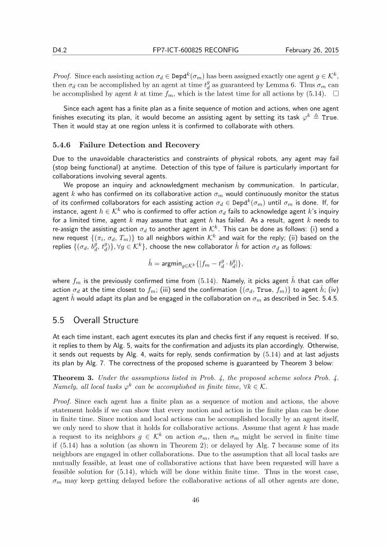
D4.2 FP7-ICT-600825 RECONFIG February 26, 2015
Proof. Since each assisting action σd ∈ Depdk(σm) has been assigned exactly one agent g ∈ Kk,then σd can be accomplished by an agent at time tgd as guaranteed by Lemma 6. Thus σm canbe accomplished by agent k at time fm, which is the latest time for all actions by (5.14).
Since each agent has a finite plan as a finite sequence of motion and actions, when one agentfinishes executing its plan, it would become an assisting agent by setting its task ϕk , True.Then it would stay at one region unless it is confirmed to collaborate with others.
5.4.6 Failure Detection and Recovery
Due to the unavoidable characteristics and constraints of physical robots, any agent may fail(stop being functional) at anytime. Detection of this type of failure is particularly important forcollaborations involving several agents.
We propose an inquiry and acknowledgment mechanism by communication. In particular,agent k who has confirmed on its collaborative action σm would continuously monitor the statusof its confirmed collaborators for each assisting action σd ∈ Depdk(σm) until σm is done. If, forinstance, agent h ∈ Kk who is confirmed to offer action σd fails to acknowledge agent k’s inquiryfor a limited time, agent k may assume that agent h has failed. As a result, agent k needs tore-assign the assisting action σd to another agent in Kk. This can be done as follows: (i) send anew request (πi, σd, Tm) to all neighbors within Kk and wait for the reply; (ii) based on thereplies (σd, bgd, t
gd), ∀g ∈ K
k, choose the new collaborator h for action σd as follows:
h = argming∈Kk|fm − tgd · bgd|,
where fm is the previously confirmed time from (5.14). Namely, it picks agent h that can offeraction σd at the time closest to fm; (iii) send the confirmation (σd, True, fm) to agent h; (iv)agent h would adapt its plan and be engaged in the collaboration on σm as described in Sec. 5.4.5.
5.5 Overall Structure
At each time instant, each agent executes its plan and checks first if any request is received. If so,it replies to them by Alg. 5, waits for the confirmation and adjusts its plan accordingly. Otherwise,it sends out requests by Alg. 4, waits for reply, sends confirmation by (5.14) and at last adjustsits plan by Alg. 7. The correctness of the proposed scheme is guaranteed by Theorem 3 below:
Theorem 3. Under the assumptions listed in Prob. 4, the proposed scheme solves Prob. 4.Namely, all local tasks ϕk can be accomplished in finite time, ∀k ∈ K.
Proof. Since each agent has a finite plan as a sequence of motion and actions, the abovestatement holds if we can show that every motion and action in the finite plan can be donein finite time. Since motion and local actions can be accomplished locally by an agent itself,we only need to show that it holds for collaborative actions. Assume that agent k has madea request to its neighbors g ∈ Kk on action σm, then σm might be served in finite timeif (5.14) has a solution (as shown in Theorem 2); or delayed by Alg. 7 because some of itsneighbors are engaged in other collaborations. Due to the assumption that all local tasks aremutually feasible, at least one of collaborative actions that have been requested will have afeasible solution for (5.14), which will be done within finite time. Thus in the worst case,σm may keep getting delayed before the collaborative actions of all other agents are done,
46
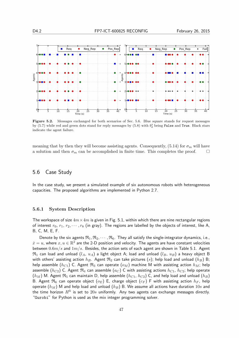
D4.2 FP7-ICT-600825 RECONFIG February 26, 2015
0 5 10 15 20 25 30 35 40Time (s)
0
1
2
3
4
5
6
7
Agen
ts
Req Neg_Rep Pos_Rep
0 5 10 15 20 25 30 35 40Time (s)
0
1
2
3
4
5
6
7
Agen
ts
Req Neg_Rep Pos_Rep Fail
Figure 5.2. Messages exchanged for both scenarios of Sec. 5.6. Blue square stands for request messagesby (5.7) while red and green dots stand for reply messages by (5.8) with bgd being False and True. Black starsindicate the agent failure.
meaning that by then they will become assisting agents. Consequently, (5.14) for σm will havea solution and then σm can be accomplished in finite time. This completes the proof.
5.6 Case Study
In the case study, we present a simulated example of six autonomous robots with heterogeneouscapacities. The proposed algorithms are implemented in Python 2.7.
5.6.1 System Description
The workspace of size 4m×4m is given in Fig. 5.1, within which there are nine rectangular regionsof interest r0, r1, r2, · · · , r8 (in gray). The regions are labelled by the objects of interest, like A,B, C, M, E, F.
Denote by the six agents R1,R2, · · · ,R6. They all satisfy the single-integrator dynamics, i.e.,x = u, where x, u ∈ R2 are the 2-D position and velocity. The agents are have constant velocitiesbetween 0.6m/s and 1m/s. Besides, the action sets of each agent are shown in Table 5.1. AgentR1 can load and unload (lA, uA) a light object A; load and unload (lB, uB) a heavy object Bwith others’ assisting action hB. Agent R2 can take pictures (s); help load and unload (hB) B;help assemble (hC1) C. Agent R3 can operate (oM ) machine M with assisting action hM ; helpassemble (hC2) C. Agent R4 can assemble (aC) C with assisting actions hC1, hC2; help operate(hM ) M. Agent R5 can maintain D, help assemble (hC1, hC2) C, and help load and unload (hB)B. Agent R6 can operate object (oE) E, charge object (cF ) F with assisting action hF , helpoperate (hM ) M and help load and unload (hB) B. We assume all actions have duration 10s andthe time horizon Hk is set to 20s uniformly. Any two agents can exchange messages directly.“Gurobi” for Python is used as the mix integer programming solver.
47

D4.2 FP7-ICT-600825 RECONFIG February 26, 2015
0.0 0.5 1.0 1.5 2.0 2.5 3.0 3.5 4.0y (m)
0.0
0.5
1.0
1.5
2.0
2.5
3.0
3.5
4.0
x (m
)
r4
r5 r6
r7
r0
r1 r2
r3
r8
Robot 1Robot 2
Robot 3Robot 4
Robot 5Robot 6
0.0 0.5 1.0 1.5 2.0 2.5 3.0 3.5 4.0y (m)
0.0
0.5
1.0
1.5
2.0
2.5
3.0
3.5
4.0
x (m
)
r4
r5 r6
r7
r0
r1 r2
r3
r8
Robot 1Robot 2
Robot 3Robot 4
Robot 5Robot 6
0.0 0.5 1.0 1.5 2.0 2.5 3.0 3.5 4.0y (m)
0.0
0.5
1.0
1.5
2.0
2.5
3.0
3.5
4.0
x (m
)
r4
r5 r6
r7
r0
r1 r2
r3
r8
Robot 1Robot 2
Robot 3Robot 4
Robot 5Robot 6
0.0 0.5 1.0 1.5 2.0 2.5 3.0 3.5 4.0y (m)
0.0
0.5
1.0
1.5
2.0
2.5
3.0
3.5
4.0
x (m
)
r4
r5 r6
r7
r0
r1 r2
r3
r8
Robot 1Robot 2
Robot 3Robot 4
Robot 5Robot 6
0.0 0.5 1.0 1.5 2.0 2.5 3.0 3.5 4.0y (m)
0.0
0.5
1.0
1.5
2.0
2.5
3.0
3.5
4.0
x (m
)
r4
r5 r6
r7
r0
r1 r2
r3
r8
Robot 1Robot 2
Robot 3Robot 4
Robot 5Robot 6
0.0 0.5 1.0 1.5 2.0 2.5 3.0 3.5 4.0y (m)
0.0
0.5
1.0
1.5
2.0
2.5
3.0
3.5
4.0
x (m
)
r4
r5 r6
r7
r0
r1 r2
r3
r8
Robot 1Robot 2
Robot 3Robot 4
Robot 5Robot 6
Figure 5.3. Snapshots of agents collaborating on actions lB , oM , uB , cF and aC . Detail descriptions are inSec. 5.6.3.
5.6.2 Task Description
Each agent is assigned a local task: agent R1 has to deliver A to r2 and B to r3. Then ϕ1 =♦(lA∧♦(r2∧©uA)
)∧♦(lB∧♦(r3∧©uB)
); Agent R2 has to surveil regions r7, r8 and take pictures
there. ϕ2 = ♦(r7∧©s)∧♦(r8∧©s); Agent R3 has to operate M and visit r6. ϕ3 = ♦(oM∧♦r6);Agent R4 has to take a photo in r7, assemble C and visit r6. ϕ4 = ♦(r7 ∧©s) ∧ ♦(aC); AgentR5 needs to maintain D and back to region r0. ϕ5 = ♦(mD ∧ ♦r0); Agent R6 needs to operateE first and then charge F. ϕ6 =©(oE ∧ ♦cF ).
5.6.3 Simulation Results
All agents start form the center (2m, 2m). The synthesized initial plan of each agent is asfollows: r0r4 lB r3 uB r1 lA r2 uA for R1; r0 r8 s r7 s for R2; r0 r8 oM r6 for R3; r0 r5 aC r7 s forR4; r0 r7mD for R5; r0 r1 oE r3cF for R6. We simulate first one nominal scenario and anotherwith R2’s failure since t = 5s. The messages exchanged during both scenarios are shown inFig. 5.2 and the simulation videos are available online [84].
Nominal Scenario
As shown in Fig. 5.3, agent R1 firstly sends the request on action hB and the reply messages areshown in Table 5.2. R2 is confirmed as the collaborator and changes its plan to r0 r4 hB r8 s r7 s.R1 finishes action lB at t = 14.3s At the same time, R4 is chosen to help R3 on action oM , whichis done at t = 21.1s. Afterwards, R1 finishes uB at t = 28.4s with R2 offering hB. Agent R6’srequest for action cF keeps getting delayed until t = 21.1s, as R2, R3, R4 are engaged in other
48

D4.2 FP7-ICT-600825 RECONFIG February 26, 2015
0.0 0.5 1.0 1.5 2.0 2.5 3.0 3.5 4.0y (m)
0.0
0.5
1.0
1.5
2.0
2.5
3.0
3.5
4.0
x (m
)
r4
r5 r6
r7
r0
r1 r2
r3
r8
Robot 1Robot 2
Robot 3Robot 4
Robot 5Robot 6
0.0 0.5 1.0 1.5 2.0 2.5 3.0 3.5 4.0y (m)
0.0
0.5
1.0
1.5
2.0
2.5
3.0
3.5
4.0
x (m
)
r4
r5 r6
r7
r0
r1 r2
r3
r8
Robot 1Robot 2
Robot 3Robot 4
Robot 5Robot 6
0.0 0.5 1.0 1.5 2.0 2.5 3.0 3.5 4.0y (m)
0.0
0.5
1.0
1.5
2.0
2.5
3.0
3.5
4.0
x (m
)
r4
r5 r6
r7
r0
r1 r2
r3
r8
Robot 1Robot 2
Robot 3Robot 4
Robot 5Robot 6
0.0 0.5 1.0 1.5 2.0 2.5 3.0 3.5 4.0y (m)
0.0
0.5
1.0
1.5
2.0
2.5
3.0
3.5
4.0
x (m
)
r4
r5 r6
r7
r0
r1 r2
r3
r8
Robot 1Robot 2
Robot 3Robot 4
Robot 5Robot 6
0.0 0.5 1.0 1.5 2.0 2.5 3.0 3.5 4.0y (m)
0.0
0.5
1.0
1.5
2.0
2.5
3.0
3.5
4.0
x (m
)
r4
r5 r6
r7
r0
r1 r2
r3
r8
Robot 1Robot 2
Robot 3Robot 4
Robot 5Robot 6
0.0 0.5 1.0 1.5 2.0 2.5 3.0 3.5 4.0y (m)
0.0
0.5
1.0
1.5
2.0
2.5
3.0
3.5
4.0
x (m
)
r4
r5 r6
r7
r0
r1 r2
r3
r8
Robot 1Robot 2
Robot 3Robot 4
Robot 5Robot 6
Figure 5.4. Snapshots of agents collaborating on actions lB , oM , uB , cF and aC for Sec. 5.6.3. Note thatR2 failed at t = 5s, instead R5 is re-assigned to assist R1 on lB , uB .
collaborations. Afterwards agent R4 is confirmed to offer action hF and cF is done at t = 38.0s.After that, agent R4 sends the request for aC regarding hC1 and hC2 . The reply messages areshown in Table 5.2. After solving (5.14), R2 and R3 offer actions hC1 and hC2 , respectively,which are done at t = 54.1s. By t = 70.3s, all agents accomplish their local tasks.
Failure Recovery
To illustrate the effectiveness of our approach for handling agent failures, we stop simulating agentR2 since t = 5s whereas the other agents remain the same. As shown in Fig. 5.4, initially agentR2 is confirmed to offer hB to R1. However since R2 fails at t = 5s, R1 detects that by theinquiry and acknowledgment mechanism described in Sec. 5.4.6 and resends a request regardinghB, for which R5 is confirmed as the new collaborator. Then lB is done at t = 22.3s. Afterwards,again with the help of R5, R1 finishes uB at t = 37.8s. R3 finishes oM with the help of R4 att = 29.7s. Before this time, agent R6 has to delay its action cF as both R3 and R4 are engagedin oM and R2 has failed. Then R3 offers hF to R6 at t = 36s. After that, R4 finishes aC withthe help of R3 and R5 at t = 68.9s. At last, each agent accomplishes its local task by t = 76.5s.
5.7 Background: Formulation of BTs
Here, we briefly introduce an overview of BTs, the reader can find a detailed description in [73].A BT is defined as a directed rooted tree where nodes are grouped into control flow nodes,execution nodes, and a root node. In a pair of connected nodes we call the outgoing node parentand the incoming node child. Then, the root node has no parents and only one child, the control
49

D4.2 FP7-ICT-600825 RECONFIG February 26, 2015
flow nodes have one parent and at least one child, and the execution nodes are the leaves of thetree (i.e. they have no children and one parent). Graphically, the children of a control flow nodeare sorted from its bottom left to its bottom right, as depicted in Figures 5.5-5.7. The executionof a BT starts from the root node. It sends ticks 1 to its child. When a generic node in a BTreceives a tick from its parent, its execution starts and it returns to its parent a status running ifits execution has not finished yet, success if its execution is accomplished (i.e. the execution endswithout failures), or failure otherwise.Here we draw a distinction between three types of control flow nodes (selector, sequence, andparallel) and between two types of execution nodes (action and condition). Their execution isexplained below.
Selector (also known as Fallback) When the execution of a selector node starts (i.e. thenode receives a tick from its parent), then the node’s children are executed in succession fromleft to right, until a child returning success or running in found. Then this message is returnedto the parent of the selector. It returns failure only when all the children return a status failure.The purpose of the selector node is to robustly carry out a task that can be performed usingseveral different approaches (e.g. a motion tracking task can be made using either a 3D cameraor a 2D camera) by performing each of them in succession until one succeeds. The graphicalrepresentation of a selector node is a box with a “?”, as in Fig. 5.5.A finite number of BTs T1, T2, . . . , TN can be composed into a more complex BT, with them aschildren, using the selector composition: T0 = Selector(T1, T2, . . . , TN ).
?
Child 1 Child 2 · · · Child N
1
Figure 5.5. Graphical representation of a selector node with N children.
Sequence When the execution of a sequence node starts, then the node’s children are executedin succession from left to right, returning to its parent a status failure (running) as soon as the achild that returns failure (running) is found. It returns success only when all the children returnsuccess. The purpose of the sequence node is to carry out the tasks that are defined by a strictsequence of sub-tasks, in which all have to succeed (e.g. a mobile robot that has to move to aregion “A” and then to a region “B”). The graphical representation of a sequence node is a boxwith a “→”, as in Fig. 5.6.A finite number of BTs T1, T2, . . . , TN can be composed into a more complex BT, with them aschildren, using the sequence composition: T0 = Sequence(T1, T2, . . . , TN ).
Parallel When the execution of a parallel node starts, then the node’s children are executed insuccession from left to right without waiting for a return status from any child before ticking the
1A tick is a signal that enables the execution of a child.
50
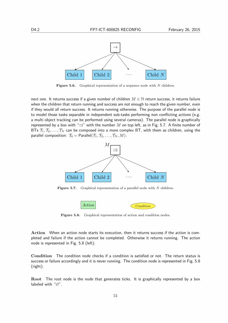
D4.2 FP7-ICT-600825 RECONFIG February 26, 2015
→
Child 1 Child 2 · · · Child N
1
Figure 5.6. Graphical representation of a sequence node with N children.
next one. It returns success if a given number of children M ∈ N return success, it returns failurewhen the children that return running and success are not enough to reach the given number, evenif they would all return success. It returns running otherwise. The purpose of the parallel node isto model those tasks separable in independent sub-tasks performing non conflicting actions (e.g.a multi object tracking can be performed using several cameras). The parallel node is graphicallyrepresented by a box with “⇒” with the number M on top left, as in Fig. 5.7. A finite number ofBTs T1, T2, . . . , TN can be composed into a more complex BT, with them as children, using theparallel composition: T0 = Parallel(T1, T2, . . . , TN ,M).
⇒M
Child 1 Child 2 · · · Child N
1
Figure 5.7. Graphical representation of a parallel node with N children.
Action
1
Condition
1
Figure 5.8. Graphical representation of action and condition nodes.
Action When an action node starts its execution, then it returns success if the action is com-pleted and failure if the action cannot be completed. Otherwise it returns running. The actionnode is represented in Fig. 5.8 (left).
Condition The condition node checks if a condition is satisfied or not. The return status issuccess or failure accordingly and it is never running. The condition node is represented in Fig. 5.8(right).
Root The root node is the node that generates ticks. It is graphically represented by a boxlabeled with “∅”.
51

D4.2 FP7-ICT-600825 RECONFIG February 26, 2015
5.8 Problem Formulation
The problem considered in this work is to define identical decentralized local BT controllers forthe single robots of a multi-robot system to achieve a global goal. We first give some assumptionsused throughout the rest of the chapter, we then state the main problem.Let S be a set of symbols describing atomic actions (e.g. perform grasp, go to position) and letR ∈ N be the set of robots in a multi-robot system, each of which can perform a finite collectionof local tasks Li ⊆ S, i ∈ R and n = |R| and let L =
⋃i∈R Li be the set of all the local tasks.
Now let G = g1, g2, . . . , gv be a finite collection of global tasks executable by the multi-robotsystem and Pk be the set of global tasks running in parallel with gk. We define ψ(gk) as the finiteset of local tasks which have to return success for the global task gk to succeed.Finally, let ν : G × L → N and µ : G × L → N respectively be functions that give the minimumnumber of robots needed, and the maximum number of robots assignable, to perform a local task,in order to accomplish a global task. Given these, we state the following assumptions:
Assumption 1. The minimum number of robots required to execute global tasks running inparallel does not exceed the total number of robots in the system:
∑gk∈Ph
∑lj∈ψ(gk) ν(gk, lj) ≤
n ∀gh ∈ G.
Assumption 2. Each global task in G can be performed by assigning to some robots in Rone of their local tasks: ψ(gk) ⊆ 2L ∀gk ∈ G.
Problem 7. Given a multi-robot system defined as above and a global goal that satisfiesAssumptions 1-2, design a local BT controller for each single robot to achieve this goal.
5.9 Proposed Solution
In this section, we will first give an informal description of the proposed solution, involving thethree subtrees TG (global tasks), TA (task assignment) and TLi(local tasks). Then, we describethe design of these subtrees in detail. To illustrate the approach we give a brief example, followedby a description of how to create a multi-agent BT from a single agent BT. Finally, we analyzethe fault tolerance of the proposed approach.
The multi-agent BT is composed of three subtrees running in parallel, returning success onlyif all three subtrees return success.
Ti = Parallel(TA, TG, TLi, 3) (5.15)
Remark 10. Note that all robots run identical copies of this tree, including computing as-signments of all robots in the team, but each robot only executes the task that they themselvesare assigned to, according to their own computation.
The first subtree, TA is doing task assignment. Parts of the performance and fault toleranceof the proposed approach comes from this feature, making sure that a broken robot is replacedand that robots are assigned to the tasks they do best.
The second subtree, TG takes care of the overall mission progression. This tree includesinformation on task that needs to be done in sequence (using sequence composition), tasks thatcould either be done in sequence or in parallel (using parallel M = N compositions), fallbacktasks that should be tried in sequence (using selector compositions), and fallbacks that can betried in parallel (using parallel M = 1 compositions). The execution of TG provides information to
52

D4.2 FP7-ICT-600825 RECONFIG February 26, 2015
the assignment in TA. The fault tolerance of the proposed approach is improved by the fallbacksencoded in TG, and the performance is improved by parallelizing actions whenever possible, asdescribed above.
The third subtree, TLi uses output from the task assignment to actually execute the properactions. We will now define the three subtrees in more detail.
Definition of TA This tree is responsible for the reactive optimal task assignment, deployingrobots to different local tasks according to the required scenario. The reactiveness lies in changesof constraints’ parameters in the optimization problem, depicting the fact that the number ofrobots needed to perform a given task changes during its execution.The assignment problem is solved using any other method used in optimization problem. Here wesuggest the following, however the user can replace the solver without changing the BT structure:
minimize -∑i∈R
∑lj∈L
p(i, lj)r(i, lj)
subject to: aj ≤∑i∈R
r(i, lj) ≤ bj ∀lj ∈ Li∑lj∈L
r(i, lj) ≤ 1 ∀i ∈ R
r(i, j) ∈ 0, 1
(5.16)
where r : R× L → 0, 1 is a function that represents the assignment of robot i to a local tasklj , taking value 1 if the assignment is done and 0 otherwise; p : R×L → R is a function assigninga performance to robot i at executing the task lj (if the robot i cannot perform the task lj i.e.,lj /∈ Li then p(i, lj) = -∞). aj , bj ∈ N are respectively the minimum and the maximum numberof robots assignable to the task lj and they change during the execution of (5.15) and aj ∈ N isset to a positive value upon requests from TG. At the beginning they are initialized to 0, since noassignment is needed. When the execution of a global task gk starts, aj and bj are set respectivelyto ν(gk, lj) and µ(gk, lj) ∀lj ∈ ψ(gk). Then when a local task lj finishes its execution (i.e., itreturns either success or failure), aj and bj decrease by 1 until aj = 0, since the robot executinglj can be assigned to another task while the other robots are still executing their local task. Whenthe task gk finishes, both aj and bj are set back to zero.The tree TA is shown in Fig. 5.9 (left). The condition “Local Task Finished” returns success if arobot has succeeded or failed a local task, failure otherwise. For ease of implementation a robotcan communicate to all the other when has finished a local task. The condition “New Global TaskExecuted” returns success if it is satisfied, failure otherwise.The condition “Check Consistency” checks if the constraints of the optimization problem are con-sistent with each other, since such constraints change their parameters during the tree execution.The addition of a constraint in (5.16) effects the system only if a solution exists. This conditionis crucial to run a number of global tasks in parallel according to the number of available robots(see Example 3 below).The action “Assign Agents” is responsible for the task assignment, it returns running while theassignment routine is executing, it returns success when the assignment problem is solved and itreturns failure if the optimal value is ∞.
53

D4.2 FP7-ICT-600825 RECONFIG February 26, 2015
Definition of TG This tree is designed to achieve the global goal defined in Problem 7 (i.e.,the global goal is achieved if the tree returns success) executing a set of global tasks.An example of TG is depicted in Fig. 5.9 (right).
→
∅
? AssignAgents
CheckConsistency
LocalTask
Finished
New GlobalTask
Executed
1
?
∅
→PerformGlobalTask g4
PerformGlobalTask g1
PerformGlobalTask g2
PerformGlobalTask g3
1
Figure 5.9. Example of BT modeling a global task
The execution of the action “Perform Global Task gk” requires that some robots have to beassigned, then it sets bj = µ(gk, lj) ∀lj ∈ ψ(gk). In the tree TA the condition “New GlobalTask Executed” is now satisfied, making a new assignment if the constraints are consistent witheach other. Finally action “Perform Global Task gk” returns success if the number of local taskslj ∈ ψ(gk) that return success is greater than ν(gk, lj) (i.e the minimum amount of robots neededhave succeeded) it returns failure if the number of local tasks in ψ(gk) that return failure is greaterthan
∑i∈R r(i, j) − ν(gk, lj) (i.e., some robots have failed to perform the task, the remaining
ones are not enough to succeed), it returns running otherwise. The case of translating a singlerobot BT to a multi robot BT is described in Section 5.9.1 below.
Definition of TLi This tree comprises the planner of a single agent. Basically it executes oneof its subtrees upon request from the TA, the request is made by executing the action “AssignAgents”.
?
∅
→
This AgentAssigned toLocal Task 1
PerformLocalTask 1
→
This AgentAssigned toLocal Task 2
PerformLocalTask 2
. . . →
This Agentis not
Assigned
Rest
1
Figure 5.10. Example of BT modeling a local task on a single agent
54

D4.2 FP7-ICT-600825 RECONFIG February 26, 2015
Example 3. By way of example, we consider a system that is to explore 2 different areas.Intuitively, different areas can be explored by different robots at the same time but if only asingle robot is available those areas can only be explored in a sequence. The local trees TLi areas depicted in Fig. 3 (below) and the global task tree TG as in Fig. 3 (above).Considering first the case in which there is only one robot available. When the executionof Explore Area A in TG starts, in (5.16) the constraint that one robot has to be assignedto explore area A is added (i.e. the related aj and bj are both set to 1). The optimizationproblem is feasible hence the assignment takes place. When the execution of Explore AreaB starts, the related constraint is not consistent with the other constraints, since the onlyavailable robot cannot be assigned to two tasks, hence the assignment does not take place.Considering now the case where a new robot is introduced in the system, it is possible toassign two robots. Both constraints: the one related to Explore Area A and the one relatedto Explore Area B, can be introduced in the optimization problem without jeopardizing itsconsistency. Those two tasks can be executed in parallel.Note that the two different executions (i.e. Explore Area A first, then Explore Area B;Explore Area A and Explore Area B in parallel) depend only on the number of availablerobots, the designed tree does not change.
⇒
∅
2
ExploreArea A
ExploreArea B
1
?
∅
→
This AgentAssigned toExplore A
Go ToArea A
→
This AgentAssigned toExplore B
Go ToArea B
→
This Agentis not
Assigned
Rest
1
Figure 5.11. Trees of example 3
5.9.1 From single robot BT to multi-robots BT
Here we present how one can design a BT for a multi-robot system reusing the BT designed tocontrol a single robot. Let TS be the tree designed for the single robot execution with AS =α1, α2, · · · being the set of action nodes, each robot in the multi-robot system will have as TGa tree with the same structure of TS changing the meaning of the action nodes and replacing thecontrol flow nodes with parallel nodes where possible.
55

D4.2 FP7-ICT-600825 RECONFIG February 26, 2015
The action nodes of TG are the global tasks G of the tree (i.e. tasks that the entire system hasto perform). Their execution has the same effect on the multi-robot system as the effect of theactions AS in TS . The execution of tasks in G adds constraints in the optimization problem ofthe tree TA defined by the sets ψ(gk), ∀gk ∈ G. Those sets, in this case, have all cardinality 1(i.e., only one robot is assigned to perform a task in G) since it is a translation from a single robotexecution to a multi-robot execution.The main advantage of having a team of robots lies in fault tolerance and the possibility of parallelexecution of some tasks. In the tree TG the user can replace sequence and selector nodes withparallel nodes and M = N and M = 1 respectively (i.e., if the children of a selector node can beexecuted in parallel, the correspondent parallel node returns success as soon as one child returnssuccess; on the other hand if the N children of a sequence node can be executed in parallel, thecorrespondent parallel node returns success only when all of them return success). The trees TLihave the same structure of the one defined in section 5.9, defining as “Perform Local Task k” theaction αk.Then to construct TG, first each action node of TS is replaced by a global task gk with ψ(gk) = αkand then the control flow nodes are replaced with parallel nodes where possible. The tree TA isalways the one defined in section 5.9.Finally, each robot i in a multi-robot system runs the tree Ti defined in (5.15).Here we observe that if the multi-robot system is heterogeneous the trees TLi are such that theyhold the condition L ⊆ AS (i.e. the multi-robot system can perform the tasks performed by theoriginal single robot).
5.9.2 Fault Tolerance
The fault tolerance capabilities of a multi-robot system are due to the redundancy of tasks exe-cutable by different robots. In particular, a local task lj can be executed by every robot i ∈ Rsatisfying the condition lj ∈ Li. Here we make the distinction between minor faults and majorfaults of a robot according to their severity. A minor fault involves a single local task lj , i.e. therobot is no longer capable to perform the task lj , here the level of a minor fault is the number oflocal tasks involved. A major fault of a robot implies that the robot can no longer perform anyof its local task.
Remark 11. A minor fault of level h is different from h minor faults, since the latter mightinvolve different robots.
Remark 12. A major fault involving a robot i ∈ R is equivalent to a minor fault of level |Li|involving every task in Li.
Definition 18. A multi-robot system is said to be weakly fault tolerant if it can tolerate anyminor fault.
Definition 19. A multi-robot system is said to be strongly fault tolerant if it can tolerateany major fault.
Lemma 7. A multi-robot system is weakly fault tolerant if and only if for each robot i ∈ Rand for each local task lj ∈ Li there exists another robot h ∈ R such that lj ∈ Li ∩ Lh andthe problem (5.16) is consistent under the constraint r(i, j) · r(h, j) = 0.
56

D4.2 FP7-ICT-600825 RECONFIG February 26, 2015
Proof. (if ) When r(i, j) · r(h, j) = 0 either robot i or h is not deployed. Assume that therobot i is involved in a minor fault, related to the local tasks lj . Since lj ∈ Li ∩ Lh, lj ∈ Lhthen the robot h can perform the local task lj in place of robot i, since it is not deployed.
(only if ) if the system can tolerate a minor fault then for each robots i there exist anotherrobot h such that the local task related to the fault can be performed by both of them sinceone took over the other. Hence lj ∈ Li and lj ∈ Lh, this implies that lj ∈ Li ∩ Lh holds.Moreover, if the fault can be tolerate it means that when lj is performed either the roboti or robot h is not deployed otherwise the reassignment would not be possible. Hence thecondition r(i, j) · r(h, j) = 0 holds.
Corollary 2. A multi-robot system can tolerate a minor fault of level h if Lemma 7 holds forthe local tasks involved in the fault.
Lemma 8. A multi-robot system is strongly fault tolerant if and only if for each robot i thereexists a set of robots I such that Li ⊆ ∪nh∈I,h 6=iLh and the problem (5.16) is consistent underthe constraints r(i, j) · r(h, j) = 0 ∀j : lj ∈ Li, h ∈ I.
Proof. (if ) Since Li ⊆ ∪h∈I,h 6=iLh all the local task of the robot i can be performed bysome other robots in the system. Then when the robot i is asked to perform a local tasklj , exists at least another robot that can perform such task, this robot is not deployed sincer(i, j) · r(h, j) = 0 ∀j : lj ∈ Li, h ∈ I.
(only if ) if the system can tolerate a major fault then exists a robot i that is redundant,i.e. its tasks can be performed by other robots. Hence exists a set of robots I, in which i isnot contained, such that Li ⊆ ∪h∈I,h 6=iLh, moreover since each local task lj of the robot i canbe performed by a robot h ∈ I, robot h is not deployed when i is performing lj otherwise itcould not take over robot i, hence r(i, j) · r(h, j) = 0 ∀j : lj ∈ Li, h ∈ I.
5.10 Motivating Example
Imagine a robot that is designed to perform maintenance on a given machine. The robot canopen and close the cover, do fault detection and replace broken hardware (HW) components.However, this robot is fairly complex and easily breaks down. Thus, it is desirable to replace thisbig versatile robot with a team of smaller specialized robots, as shown in Figure 5.12.
More concretely, we assume that the multi-robot system is designed to replace damaged partsof the electronic hardware of a vehicle. Let us assume that to repair the vehicle, the system hasto open the metal cover first, then it has to check which parts have been damaged, replace thedamaged parts, solder the connecting wires, and finally close the metal cover. In this examplethe setup is given by a team composed by robots of type A, B and C. Robots of type A aresmall mobile dual arm robots that can carry spare hardware pieces, place them and remove thedamaged part from the vehicles, and do diagnosis. Robots of type B are also small mobile dualarm robots with a gripper and soldering iron as end effectors. Robots of type C are big dual armrobots that can remove and fasten the vehicle cover. We consider the general case in which thevehicle’s electronic hardware consists of p parts, all of them replaceable. The global tasks set is
57

D4.2 FP7-ICT-600825 RECONFIG February 26, 2015
C
REST
C
REST
HW1
A
REPLACEHW
A
FAULT
B
REPLACEHW
B
REST
HW1 HW2 HW3 HW4 HW5
Figure 5.12. Snapshot of a multi-robot mission execution. Two robots are replacing the broken parts, HW2and HW4, (bottom) of a machine. One robot is out of order (top left), and tree robots are resting (top right).
defined as:
G =Normal Operating Condition,Open Metal Cover,
Close Metal Cover,Fix Part 1,Fix Part 2, . . . ,Fix Part p,
Diagnose Part 1,Diagnose Part 2, . . . ,Diagnose Part p.(5.17)
where:
Open Metal Cover =Remove Screws,Remove CoverClose Metal Cover =Place Screws,Place Cover
Fix Part k =Fix HW k,Fix Wires k,
Solder k k = 1, 2, . . . , p.
(5.18)
The global tasks for robots of type A set are:
Li =Replace HW,Replace Wires,Do Diagnosis on ki = 1, 2.
(5.19)
The global tasks for robots of type B set are:
Li =Replace HW,Replace Wires,
Do Diagnosis on k,Solder i = 3, 4.(5.20)
The global tasks for robots of type C set are:
Li =Use Screwdriver,Move Frame i = 5, 6. (5.21)
58

D4.2 FP7-ICT-600825 RECONFIG February 26, 2015
The map from global tasks to local tasks ψ are as follows:
ψ(Remove Screws) = Use Screwdriver
ψ(Place Screws) = Use Screwdriver
ψ(Remove Cover) = Move frame
ψ(Place Cover) = Move frame
ψ(Diagnose Part k) = Do Diagnosis on k
ψ(Fix HW k) = Replace HW k
ψ(Fix Wires k) = Replace Wires k
ψ(Solder k) = Use Soldering Iron on k
(5.22)
The tree TG defined is showed in Fig. 5.13.
→
RemoveScrews
RemoveCover
PlaceScrews
Place Cover
∅
?
NominalOperatingConditions
⇒p
?
DiagnosePart 1
?
DiagnosePart 2
· · · ?
DiagnosePart p
→
FixHW 1
FixWires 1
Solder1
→
FixHW 2
FixWires 2
Solder2
→
FixHW p
FixWires p
Solderp
1
Figure 5.13. TG of Example 5.10
5.10.1 Execution
Here we describe the execution of the above mission using the proposed framework.Consider a team of 2 robots of type A, 2 robots of type B, and 2 robots of type C designate todiagnose and fix a vehicle composed by 5 critical parts as depicted in Fig. 5.14(a). The robots’performances p(i, lj) are related to how fast tasks are accomplished. They are collected in Ta-ble 5.3, and the scenario’s parameters are in Table 5.4.
When the vehicle is running on nominal operating conditions, the assignment tree TA of eachrobot has aj = bj = 0 since no assignments are needed. When a fault on the vehicle takes place,the condition “Nominal Operating Conditions” is no longer true in all the robots’ BTs, then the“Remove Screws” action has to be executed. According to ψ(Remove Screws) this global taskrequires the local task “Use Screwdriver” to be accomplished. The constraints related to this task
59

D4.2 FP7-ICT-600825 RECONFIG February 26, 2015
Task Robots A Robots B Robots C
Use Screwdriver -∞ -∞ 1
Move Frame -∞ -∞ 1
Do Diagnosis on k 3 1 -∞Replace HW k 1.5 1 -∞Replace Wires k 1.5 1 -∞Use Soldering Iron on k -∞ 1 -∞
Table 5.3. Robot performances values
have to be added in (5.16) after checking the feasibility of the optimization problem. The parame-ter aj and bj for “Use Screwdriver” are changed into: aj = ν(Remove Screws, Use Screwdriver) =1 and bj = µ(Remove Screws, Use Screwdriver) = 2 with j : lj = Use Screwdriver. Solv-ing (5.16) both robots C are assigned to “Use Screwdriver”, while the other are not deployed(Fig. 5.14(b)). When a robot accomplishes its local task, then the corresponding bj is de-creased by 1 until bj = 0 and the robot can be deployed for a new task if needed. A sim-ilar assignment is then made to accomplish the global task “Remove Cover”. After removingthe metal cover, all the vehicle hardware have to be diagnosed, and the global task “DiagnosePart 1” will change the parameters in aj = ν(Diagnose Part 1, Do Diagnosis on 1) = 1 andbj = µ(Diagnose Part 1, Do Diagnosis on 1) = 1 with j : lj = Do Diagnosis on 1, in a similarway “Diagnose Part 2” will change the parameters in aj = ν(Diagnose Part 2, Do Diagnosis) = 1and bj = µ(Diagnose Part 2, Do Diagnosis) = 1 with j : lj = Do Diagnosis and so forth until“Diagnose Part 4”. When the system changes the parameters related to “Diagnose Part 5” theoptimization problem is not feasible since there are not enough agents, then the assignment for“Diagnose Part 5” does not take place (Fig. 5.14(c)).Here we show the reactive functionality of the proposed framework. Note that the robots of typeA have higher performance than the robots of type B in doing diagnosis according to Table 5.3,i.e., they are faster. While the robots of type B are still doing diagnosis on HW3 and HW4, therobots of type A can be deployed for new tasks without waiting for the slower robots (Fig. 5.14(d)).After diagnosis, HW2 and HW4 must be replaced, robots of type A have higher performance in“Replace HW” therefore, they are deployed to minimize the objective function of (5.16), robots oftype B are not deployed since µ(Fix HW k, Replace HW k) = 1 i.e. the replacing of an electronicHW is made by a single robot (Fig. 5.14(e)).If a robot of type A has a major fault, all its performance parameters are set to -∞ and arobot of type B can take over since it can execute all the task of a robot A, this situationis depicted in Fig. 5.14(f). Here two robots of type B are replacing wires on HW1, sinceµ(Fix Part i, Replace Wires) = 2 and a robot of type A is replacing wires on HW2. The fi-nal part of the repair is the soldering of the new wires, executable only by robots of type B(Fig. 5.14(g)). Finally the metal cover is put back (Fig. 5.14(h)) and the tree TG returns success.
5.10.2 Fault Tolerance Analysis
Analyzing the system, it is neither weakly nor strongly fault tolerant. A minor fault on the localtask “Move Frame” can not be tolerated since ν(Remove Cover, Move Frame) = 2 as well asν(Place Cover, Move Frame) = 2 thus a single robot cannot perform the task. However, somefaults can be tolerated. The multi-robot system can tolerate up to 3 major faults (2 faults involving
60

D4.2 FP7-ICT-600825 RECONFIG February 26, 2015
Patameter Value
ν(Remove Screws, Use Screwdriver) 1
µ(Remove Screws, Use Screwdriver) 2
ν(Place Screws, Use Screwdriver) 1
µ(Place Screws, Use Screwdriver) 2
ν(Remove Cover, Move Frame) 2
µ(Remove Cover, Move Frame) 2
ν(Place Screws, Remove Cover) 1
µ(Place Screws, Remove Cover) 2
ν(Place Cover, Move Frame) 2
µ(Place Cover, Move Frame) 2
ν(Diagnose Part k, Do Diagnosis on k) 1
µ(Diagnose Part k, Do Diagnosis on k) 1
ν(Fix HW k, Replace HW k) 1
µ(Fix HW k, Replace HW k) 1
ν(Fix Wires k, Replace Wires k) 1
µ(Fix Wires k, Replace Wires k) 2
ν(Solder k, Use Soldering Iron on k) 1
µ(Solder k, Use Soldering Iron on k) 3
Table 5.4. Scenario parameters. Note that when ν = µ, as in the case of (Remove Cover, Move Frame)we have that the number of required robots for a task is equal to the maximal number of robots that canparticipate in executing the task.
both robots A, and 1 fault involving a robot B) and up to 11 minor fault (1 fault involving “UseScrewdriver”, 3 faults involving “Replace HW k”, 3 faults involving “Replace Wires k”, and 3faults involving “Do diagnosis on k” ), as long as at least one robot of type B and 2 robots oftype C are operating. Note that the local task “Use soldering iron on k” can be performed by arobot of type B only.
5.11 Summary
In the first part of the chapter, we presented a bottom-up distributed motion and task coordinationscheme for multi-agent systems with dependent local tasks assigned to the individual agents.This framework relies on the off-line initial plan synthesis, the on-line request and reply messagesexchange protocol, and the real-time plan adaptation algorithm. In the second part, we exploitedBTs as a possibility to design distributed controllers for multi-robot systems working towardsglobal goals and improve their performance and fault tolerance.
61

D4.2 FP7-ICT-600825 RECONFIG February 26, 2015
A
REST
A
REST
B
REST
B
REST
C
REST
C
REST
HW1HW1 HW2 HW3 HW2 HW1
(a) Screenshot I
A
REST
A
REST
B
REST
B
REST
HW1
C
USESCREW-DRIVER
C
USESCREW-DRIVER
HW1 HW2 HW3 HW4 HW5
(b) Screenshot II
C
REST
C
REST
HW1
A
DIAGNOSE
A
DIAGNOSE
B
DIAGNOSE
B
DIAGNOSE
HW1 HW2 HW3 HW4 HW5
(c) Screenshot III
C
REST
C
REST
HW1
A
DIAGNOSE
A
REPLACEHW
B
DIAGNOSE
B
DIAGNOSE
HW1 HW2 HW3 HW4 HW5
(d) Screenshot IV
C
REST
C
REST
HW1
A
REPLACEHW
A
REPLACEHW
B
REST
B
REST
HW5 HW2 HW3 HW4 HW5
(a) Screenshot V
C
REST
C
REST
HW1
A
REPLACEHW
A
FAULT
B
REPLACEHW
B
REST
HW1 HW2 HW3 HW4 HW5
(b) Screenshot VI
C
REST
C
REST
HW1
A
REST
A
FAULT
B
USESOLDERING
IRON
B
USESOLDERING
IRON
HW1 HW2 HW3 HW4 HW5
(c) Screenshot VII
HW1
A
REST
A
FAULT
B
REST
B
REST
HW1 HW2 HW3 HW4 HW5
C
USESCREW-DRIVER
C
USESCREW-DRIVER
(d) Screenshot VIII
Figure 5.14. Plan Execution. HW components are either un-diagnosed (grey), checked and OK (green) orbroken (red)
62

Bibliography
[1] M. Aicardi, G. Casalino, A. Bicchi, and A. Balestrino. Closed loop steering of unicycle-likevehicles via lyapunov techniques, IEEE Robotics and Automation Magazine, 2(1):27–35,1995.
[2] Extended version. http://arxiv.org/abs/1405.1836.
[3] J. A. D. Bagnell, F. Cavalcanti, L. Cui, T. Galluzzo, M. Hebert, M. Kazemi, M. Klingensmith,J. Libby, T. Y. Liu, N. Pollard, M. Pivtoraiko, J.-S. Valois, and R. Zhu. An Integrated Systemfor Autonomous Robotics Manipulation, in IEEE/RSJ International Conference on IntelligentRobots and Systems, pages 2955–2962, October 2012.
[4] C. Baier and J.-P. Katoen. Principles of Model Checking. MIT Press, 2008.
[5] T. Balch and R. C. Arkin. Communication in reactive multiagent robotic systems, Au-tonomous Robots, 1(1): 1–25, 1994.
[6] C. P. Bechlioulis and G. A. Rovithakis. Robust adaptive control of feedback linearizable mimononlinear systems with prescribed performance, IEEE Transactions on Automatic Control,53(9): 2090–2099, 2008.
[7] C. Belta, A. Bicchi, M. Egerstedt, E. Frazzoli, E. Klavins, G. J. Pappas. Symbolic planningand control of robot motion. IEEE Robotics and Automation Magazine, 14(1): 61–70, 2007.
[8] A. Bhatia, L. E. Kavraki, M. Y. Vardi. Sampling-based motion planning with temporal goals.IEEE International Conference on Robotics and Automation(ICRA), 2689–2696, 2010.
[9] A. Bhatia, M. R. Maly, L. E. Kavraki, and M. Y. Vardi. Motion planning with complex goals,Robotics Automation Magazine, IEEE, 18(3): 55 –64, 2011.
[10] I. Bojic, T. Lipic, M. Kusek, and G. Jezic. Extending the JADE Agent Behaviour Modelwith JBehaviourtrees Framework, in Agent and Multi-Agent Systems: Technologies andApplications. Springer, pages 159–168, 2011.
[11] R. G. Brown and J. S. Jennings. A pusher/steerer model for strongly cooperative mobile robotmanipulation, in Proceedings of the IEEE International Conference on Intelligent Robots andSystems, vol. 3, pages 562–568, 1995.
[12] C. Castelfranchi and R. Falcone. Towards a Theory of Delegation for Agent-based Systems,Robotics and Autonomous Systems, 24: 141–157, 1998.
63

D4.2 FP7-ICT-600825 RECONFIG February 26, 2015
[13] L. I. R. Castro, P. Chaudhari, J. Tumova, S. Karaman, E. Frazzoli, and D. Rus. Incrementalsampling-based algorithm for minimum-violation motion planning, in Proceedings of the IEEEConference on Decision and Control (CDC), pages 3217–3224, 2013.
[14] S. Chaki, E. M. Clarke, J. Ouaknine, N. Sharygina, and N. Sinha. State/event-based softwaremodel checking, in Integrated Formal Methods. Springer, pages 128–147, 2004.
[15] A. Champandard, Understanding Behavior Trees. AiGameDev. com, vol. 6, 2007.
[16] Y. Chen, X. C. Ding, A. Stefanescu, and C. Belta. Formal approach to the deployment ofdistributed robotic teams. IEEE Transactions on Robotics, 28(1): 158–171, 2012.
[17] S. Chinchali, S. C. Livingston, U. Topcu, J. W. Burdick, and R. M. Murray. Towards formalsynthesis of reactive controllers for dexterous robotic manipulation, in Proceedings of theIEEE International Conference on Robotics and Automation (ICRA), pages 5183–5189, 2012.
[18] M. Colledanchise, A. Marzinotto, D. V. Dimarogonas and P. Ogren. Adaptive Fault TolerantExecution of Multi-Robot Missions using Behavior Trees. Submitted.
[19] M. Colledanchise, A. Marzinotto, and P. Ogren. Performance Analysis of Stochastic BehaviorTrees, in Robotics and Automation (ICRA), 2014 IEEE International Conference on, June2014.
[20] E. W. Dijkstra. Letters to the editor: go to statement considered harmful, Commun. ACM,vol. 11, pages 147–148, March 1968. [Online]. Available: http://doi.acm.org/10.1145/
362929.362947
[21] D. V. Dimarogonas and K. J. Kyriakopoulos. A connection between formation control andflocking behavior in nonholonomic multiagent systems. IEEE International Conference onRobotics and Automation(ICRA), pages 940–945, 2006.
[22] X. Ding, M. Kloetzer, Y. Chen, C. Belta. Automatic deployment of robotic teams. IEEERobotics Automation Magazine, 18: 75–86, 2011.
[23] P. Doherty, D. Landn, and F. Heintz. A distributed task specification language for mixed-initiative delegation, 2012.
[24] B. Donald, On information invariants in robotics. Artificial Intelligence, 72(1-2): 217–304,1995.
[25] M. B. Egerstedt and X. Hu. Formation constrained multi-agent control. Georgia Institute ofTechnology, 2001.
[26] G. E. Fainekos, A. Girard, H. Kress-Gazit, and G. J. Pappas. Temporal logic motion planningfor dynamic robots, Automatica, 45(2): 343–352, 2009.
[27] R. Falcone and C. Castelfranchi. C.: The human in the loop of a delegated agent: The theoryof adjustable social autonomy, IEEE Transactions on Systems, Man and CyberneticsPart A:Systems and Humans, pages 406–418, 2001.
[28] I. Filippidis, D. V. Dimarogonas, and K. J. Kyriakopoulos. Decentralized multi-agent controlfrom local LTL specifications. IEEE Conference on Decision and Control (CDC), pages 6235–6240, 2012.
64

D4.2 FP7-ICT-600825 RECONFIG February 26, 2015
[29] J. G, C. Finucane, V. Raman, and H. Kress-Gazit. Correct high-level robot control fromstructured english, in Proceedings of the IEEE International Conference on Robotics andAutomation (ICRA), pages 3543–3544, 2012.
[30] H. Garcia-Molina. Elections in a distributed computing system. IEEE Transactions on Com-puters, 31(1): 48–59, 1982.
[31] P. Gastin, D. Oddoux. Fast LTL to Buchi automaton translation. International Conferenceon Computer Aided Verification, 2001.
[32] P. Gastin and D. Oddoux. LTL2BA tool, viewed September 2012. URL: http://www.lsv.ens-cachan.fr/ gastin/ltl2ba/.
[33] B. P. Gerkey and M. J. Mataric. Sold!: Auction methods for multirobot coordination. IEEETransactions on Robotics and Automation, 18(5): 758–768, 2002.
[34] R. Gerth, D. Peled, M. Y. Vardi, and P. Wolper. Simple on-the-fly automatic verification oflinear temporal logic, in Proceedings of the Fifteenth IFIP WG6. 1 International Symposiumon Protocol Specification, Testing and Verification. IFIP, 1995.
[35] M. Guo, K. H. Johansson and D. V. Dimarogonas. Motion and Action Planning under LTLSpecification using Navigation Functions and Action Description Language. IEEE/RSJ Inter-national Conference on Intelligent Robots and Systems(IROS), pages 240–245, 2013.
[36] M. Guo, K. H. Johansson, and D. V. Dimarogonas. Revising motion planning under lin-ear temporal logic specifications in partially known workspaces, in Proceedings of the IEEEInternational Conference on Robotics and Automation (ICRA), pages 5010–5017, 2013.
[37] M. Guo and D. V. Dimarogonas. Reconfiguration in motion planning of single- and multi-agent systems under infeasible local LTL specifications. IEEE Conference on Decision andControl(CDC), pages 2758–2763, 2013.
[38] M. Guo and D. V. Dimarogonas. Distributed plan reconfiguration via knowledge transferin multi-agent systems under local LTL specifications. IEEE International Conference onRobotics and Automation (ICRA), pages 4304–4309, 2014.
[39] M. Guo, and D. V. Dimarogonas. Bottom-up Multi-agent Motion and Task Coordinationfrom Dependent Local Tasks. Submitted.
[40] M. Guo, K. H. Johansson, and D. V. Dimarogonas. Motion and action planning under LTLspecifications using navigation functions and action description language, in IEEE/RSJ In-ternational Conference on Intelligent Robots and Systems (IROS), pages 240–245, 2013.
[41] M. Guo, J. Tumova, and D. V. Dimarogonas. Cooperative decentralized multi-agent controlunder local LTL tasks and connectivity constraints. IEEE Conference on Decision and Control(CDC), 2014.
[42] Y. Hong, J. Hu, and L. Gao. Tracking control for multi-agent consensus with an active leaderand variable topology. Automatica, 42(7): 1177–1182, 2006.
[43] R. A. Horn and C. R. Johnson. Matrix analysis. Cambridge university press, 2012.
65
D4.2 FP7-ICT-600825 RECONFIG February 26, 2015
[44] D. Isla. Handling Complexity in the Halo 2 AI,in Game Developers Conference, 2005.
[45] D. Isla. Halo 3-building a Better Battle, in Game Developers Conference, 2008.
[46] S. Karaman and E. Frazzoli. Vehicle routing problem with metric temporal logic specifications,in IEEE Conference on Decision and Control(CDC), pages 3953–3958, 2008.
[47] S. Karaman, E. Frazzoli. Vehicle routing with linear temporal logic specifications: Applicationsto Multi-UAV Mission Planning. Navigation, and Control Conference in AIAA Guidance, 2008.
[48] S. Karaman and E. Frazzoli. Vehicle routing with temporal logic specifications: Applicationsto multi-UAV mission planning. International Journal of Robust and Nonlinear Control,21:1372–1395, 2011.
[49] S. Karaman and E. Frazzoli. Sampling-based optimal motion planning with deterministicµ-calculus specifications, in Proceedings of the American Control Conference (ACC), pages735–742, 2012.
[50] R. J. Kenefic and A. H. Nuttall. Maximum likelihood estimation of the parameters of a toneusing real discrete data, IEEE Journal of Oceanic Engineering, 12(1): 279–280, 1987.
[51] H. K. Khalil and J. W. Grizzle. Nonlinear systems, volume 3. Prentice hall Upper SaddleRiver, 2002.
[52] O. Khatib. Object manipulation in a multi-effector robot system, in Proceedings of the 4thInternational Symposium on Robotics Research, vol. 4. MIT Press, pages 137–144, 1988.
[53] O. Khatib, K. Yokoi, K. Chang, D. Ruspini, R. Holmberg, and A. Casal. Vehicle/arm co-ordination and multiple mobile manipulator decentralized cooperation, in in proceedings ofthe IEEE International Conference on Intelligent Robots and Systems, vol. 2, pages 546–553,1996.
[54] K. Kim and G. Fainekos. Approximate solutions for the minimal revision problem of speci-fication automata, in Proceedings of the IEEE/RSJ International Conference on IntelligentRobots and Systems (IROS), 2012.
[55] M. Kloetzer, X. C. Ding, and C. Belta. Multi-robot deployment from ltl specifications withreduced communication. IEEE Conference on Decision and Control and European ControlConference(CDC-ECC), pages 4867–4872, 2011.
[56] M. Kloetzer and C. Belta. Managing non-determinism in symbolic robot motion planning andcontrol, in Proceedings of the IEEE International Conference on Robotics and Automation(ICRA), 2007.
[57] A. Klokner. Interfacing Behavior Trees with the World Using Description Logic, in AIAAconference on Guidance, Navigation and Control, Boston, 2013.
[58] K. Kosuge, T. Oosumi, M. Satou, K. Chiba, and K. Takeo. Transportation of a single objectby two decentralized-controlled nonholonomic mobile robots, in Proceedings of the IEEEInternational Conference on Robotics and Automation, 4:2989–2994, 1998.
[59] S. Kraus. Negotiation and cooperation in multi-agent environments. Artificial Intelligence,94(1):79-97, 1997.
66

D4.2 FP7-ICT-600825 RECONFIG February 26, 2015
[60] H. Kress-Gazit, G. E. Fainekos, and G. J. Pappas. Temporal-logic-based reactive mission andmotion planning, IEEE Transactions on Automatic Control, 25(6):1370–1381, 2009.
[61] H. Kress-Gazit, T. Wongpiromsarn and U. Topcu. Correct, reactive robot control from ab-straction and temporal logic specifications. IEEE Robotics and Automation Magazine, 18(3):65-74, 2011.
[62] O. Kupferman and M. Y. Vardi. Model checking of safety properties. Formal Methods inSystem Design, 19:291–314, 2001.
[63] M. Lahijanian, J. Wasniewski, S. B. Andersson, and C. Belta. Motion planning and controlfrom temporal logic specifications with probabilistic satisfaction guarantees, in Proceedings ofthe IEEE International Conference on Robotics and Automation (ICRA), pages 3227 –3232,2010.
[64] S. M. LaValle. Planning algorithms. Cambridge University Press, 2006.
[65] C. E. Leiserson, R. L. Rivest, C. Stein, and T. H. Cormen. Introduction to algorithms. MITpress, 2001.
[66] C. Lim, R. Baumgarten, and S. Colton. Evolving Behaviour Trees for the Commercial GameDEFCON, Applications of Evolutionary Computation, pages 100–110, 2010.
[67] S. G. Loizou, K. J. Kyriakopoulos. Automatic synthesis of multi-agent motion tasks based onLTL specifications. IEEE Conference on Decision and Control(CDC), pages 153–158, 2004.
[68] S. G. Loizou and K. J. Kyriakopoulos. Automated planning of motion tasks for multi-robotsystems. IEEE Conference on Decision and Control (CDC), pages 78–83, 2005.
[69] J. Lygeros, F. Ramponi, and C. Wiltsche. Synthesis of an asynchronous communicationprotocol for search and rescue robots. European Control Conference (ECC), pages 1256–1261, 2013.
[70] M. R. Maly, M. Lahijanian, L. E. Kavraki, H. Kress-Gazit, and M. Y. Vardi. Iterative temporalmotion planning for hybrid systems in partially unknown environments, in Proceedings of the16th International Conference on Hybrid Systems: Computation and Control (HSCC). ACM,pages 353–362, 2013.
[71] A. Marzinotto, M. Colledanchise, C. Smith, and P. Ogren. Towards a Unified Behavior TreesFramework for Robot Control, in Robotics and Automation (ICRA), 2014 IEEE InternationalConference on, June 2014.
[72] A. Marzinotto, M. Colledanchise, and I. Tjernberg. (2013) Behavior trees library for the robotoperating system (ROS). [Online]. Available: https://github.com/almc/behavior_
trees
[73] P. Ogren. Increasing Modularity of UAV Control Systems using Computer Game BehaviorTrees, in AIAA Guidance, Navigation and Control Conference, Minneapolis, MN, 2012.
[74] G. Pereira, B. Pimentel, L. Chaimowicz, and M. Campos. Coordination of multiple mobilerobots in an object carrying task using implicit communication, in Proceedings of the IEEEInternational Conference on Robotics and Automation, vol. 1, pages 281–286, 2002.
67

D4.2 FP7-ICT-600825 RECONFIG February 26, 2015
[75] D. Perez, M. Nicolau, M. O’Neill, and A. Brabazon. Evolving Behaviour Trees for the MarioAI Competition Using Grammatical Evolution, Applications of Evolutionary Computation,2011.
[76] E. Plaku, L. E. Kavraki, and M. Y. Vardi. Motion planning with dynamics by a synergisticcombination of layers of planning, IEEE Transactions on Robotics, 26(3):469 – 482, 2010.
[77] I. Pohl. Bi-directional search. IBM TJ Watson Research Center, 1970.
[78] M. M. Quottrup, T. Bak, and R. I. Zamanabadi. Multi-robot planning: a timed automataapproach. IEEE International Conference on Robotics and Automation (ICRA), pages 4417–4422, 2004.
[79] W. Ren. Multi-vehicle consensus with a time-varying reference state. Systems & ControlLetters, 56(7): 474–483, 2007.
[80] I. Saha, R. Ramaithitima, V. Kumar, G. Pappas, and S. Seshia. Automated composition ofmotion primitives for multi-robot systems from safe LTL specifications. IEEE/RSJ Interna-tional Conference on Intelligent Robots and Systems (IROS), pages 1525 – 1532, 2014.
[81] V. Schuppan and A. Biere. Shortest counterexamples for symbolic model checking of LTLwith past, in Tools and Algorithms for the Construction and Analysis of Systems, ser. LectureNotes in Computer Science. Springer Berlin Heidelberg, vol. 3440, pages 493–509, 2005.
[82] A. Shoulson, F. M. Garcia, M. Jones, R. Mead, and N. I. Badler. Parameterizing BehaviorTrees, in Motion in Games. Springer, 2011.
[83] Simulation. https://www.dropbox.com/s/yhyueagokeihv7k/simulation.avi.
[84] Simulation videos. https://drive.google.com/foldervie
w?id=0B3YLWjQD8hZhWjI2cUlKSlUxT0E&usp=sharing
[85] S. L. Smith, J. Tumova, C. Belta, and D. Rus. Optimal Path Planning for Surveillance withTemporal Logic Constraints, International Journal of Robotics Research, 30(14):1695–1708,2011.
[86] E. D. Sontag. Mathematical Control Theory. London, U.K.: Springer, 1998.
[87] D. J. Stilwell and J. S. Bay. Toward the development of a material transport system usingswarms of ant-like robots, in Proceedings of the IEEE International Conference on Roboticsand Automation, vol. 1, pages 766–771, 1993.
[88] D. J. Stilwell and B. E. Bishop. Framework for decentralized control of autonomous vehicles,in Proceedings of the IEEE International Conference on Robotics and Automation, vol. 3,pages 2358–2363, 2000.
[89] T. Sugar and V. Kumar. Decentralized control of cooperating mobile manipulators, in Pro-ceedings of the IEEE International Conference on Robotics and Automation, vol. 4, pages2916–2921, 1998.
[90] C. Tang, R. Bhatt, and V. Krovi. Decentralized kinematic control of payload transport bya system of mobile manipulators, in Proceedings of the IEEE International Conference onRobotics and Automation, pages 2462–2467, 2004.
68

D4.2 FP7-ICT-600825 RECONFIG February 26, 2015
[91] H. Tanner, S. Loizou, and K. Kyriakopoulos. Nonholonomic navigation and control of coop-erating mobile manipulators, IEEE Transactions on Robotics and Automation, 19(1): 53–64,2003.
[92] A. Tsiamis, J. Tumova, C. P. Bechlioulis, G. C. Karras, D. V. Dimarogonas and K. J.Kyriakopoulos. Execution of LTL plans in leader-follower schemes without any explicit com-munication. Submitted.
[93] J. Tumova and D. V. Dimarogonas. A receding horizon approach to multi-agent planningfrom LTL specifications. American Control Conference (ACC), pages 1775–1780, 2014.
[94] J. Tumova, A. Marzinotto, D. V. Dimarogonas and D. Kragic. Maximally Satisfying LTLAction Planning, in IEEE/RSJ International Conference on Intelligent Robots and Systems,Chicago, Illinois, September 2014
[95] J. Tumova, G. C. Hall, S. Karaman, E. Frazzoli, and D. Rus. Least-violating control strategysynthesis with safety rules, in Proceedings of the 16th International Conference on HybridSystems: Computation and Control (HSCC). ACM, pages 1–10, 2013.
[96] A. Ulusoy, S. L. Smith, and C. Belta. Optimal multi-robot path planning with ltl constraints:Guaranteeing correctness through synchronization, CoRR, vol. abs/1207.2415, 2012.
[97] A. Ulusoy, S. L. Smith, X. C. Ding, C. Belta, and D. Rus. Optimality and robustness inmulti-robot path planning with temporal logic constraints. International Journal of RoboticsResearch, 32(8): 889–911, 2013.
[98] C. Wiltsche, F. A. Ramponi, and J. Lygeros. Synthesis of an asynchronous communicationprotocol for search and rescue robots. European Control Conference (ECC), pages 1256–1261, 2013.
[99] E. M. Wolff, U. Topcu, and R. M. Murray. Optimal control of non-deterministic systems for acomputationally efficient fragment of temporal logic, in Proceedings of the IEEE Conferenceon Decision and Control (CDC), pages 3197–3204, 2013.
[100] L. A. Wolsey. Integer Programming. New York: Wiley, 1998.
[101] T. Wongpiromsarn, U. Topcu, and R. M. Murray. Receding horizon control for temporallogic specifications. 13th ACM International Conference on Hybrid Systems: Computationand Control, pages 101-110, 2010.
[102] T. Wongpiromsarn, U. Topcu, and R. Murray. Receding horizon temporal logic planning,IEEE Transactions on Automatic Control, 57(11):2817–2830, 2012.
69