Embed Size (px)
Citation preview

Effect of a sub-horizontal fracture zone and rock mass heterogeneity on the stress field in Forsmark area – A numerical study using 3DEC
Preliminary site description Forsmark area – version 1.2
Diego Mas Ivars, Hossein Hakami
Itasca Geomekanik AB
September 2005
R-05-59
Svensk Kärnbränslehantering ABSwedish Nuclear Fueland Waste Management CoBox 5864SE-102 40 Stockholm Sweden Tel 08-459 84 00 +46 8 459 84 00Fax 08-661 57 19 +46 8 661 57 19

Effect of a sub-horizontal fracture zone and rock mass heterogeneity on the stress field in Forsmark area – A numerical study using 3DEC
Preliminary site descriptionForsmark area – version 1.2
Diego Mas Ivars, Hossein Hakami
Itasca Geomekanik AB
September 2005
ISSN 1402-3091
SKB Rapport R-05-59
This report concerns a study which was conducted for SKB. The conclusions and viewpoints presented in the report are those of the authors and do not necessarily coincide with those of the client.
A pdf version of this document can be downloaded from www.skb.se
3
Summary
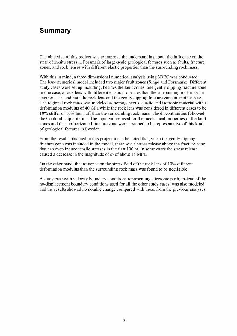
The objective of this project was to improve the understanding about the influence on the state of in-situ stress in Forsmark of large-scale geological features such as faults, fracture zones, and rock lenses with different elastic properties than the surrounding rock mass.
With this in mind, a three-dimensional numerical analysis using 3DEC was conducted. The base numerical model included two major fault zones (Singö and Forsmark). Different study cases were set up including, besides the fault zones, one gently dipping fracture zone in one case, a rock lens with different elastic properties than the surrounding rock mass in another case, and both the rock lens and the gently dipping fracture zone in another case. The regional rock mass was modeled as homogeneous, elastic and isotropic material with a deformation modulus of 40 GPa while the rock lens was considered in different cases to be 10% stiffer or 10% less stiff than the surrounding rock mass. The discontinuities followed the Coulomb slip criterion. The input values used for the mechanical properties of the fault zones and the sub-horizontal fracture zone were assumed to be representative of this kind of geological features in Sweden.
From the results obtained in this project it can be noted that, when the gently dipping fracture zone was included in the model, there was a stress release above the fracture zone that can even induce tensile stresses in the first 100 m. In some cases the stress release caused a decrease in the magnitude of σ1 of about 18 MPa.
On the other hand, the influence on the stress field of the rock lens of 10% different deformation modulus than the surrounding rock mass was found to be negligible.
A study case with velocity boundary conditions representing a tectonic push, instead of the no-displacement boundary conditions used for all the other study cases, was also modeled and the results showed no notable change compared with those from the previous analyses.
4
Sammanfattning
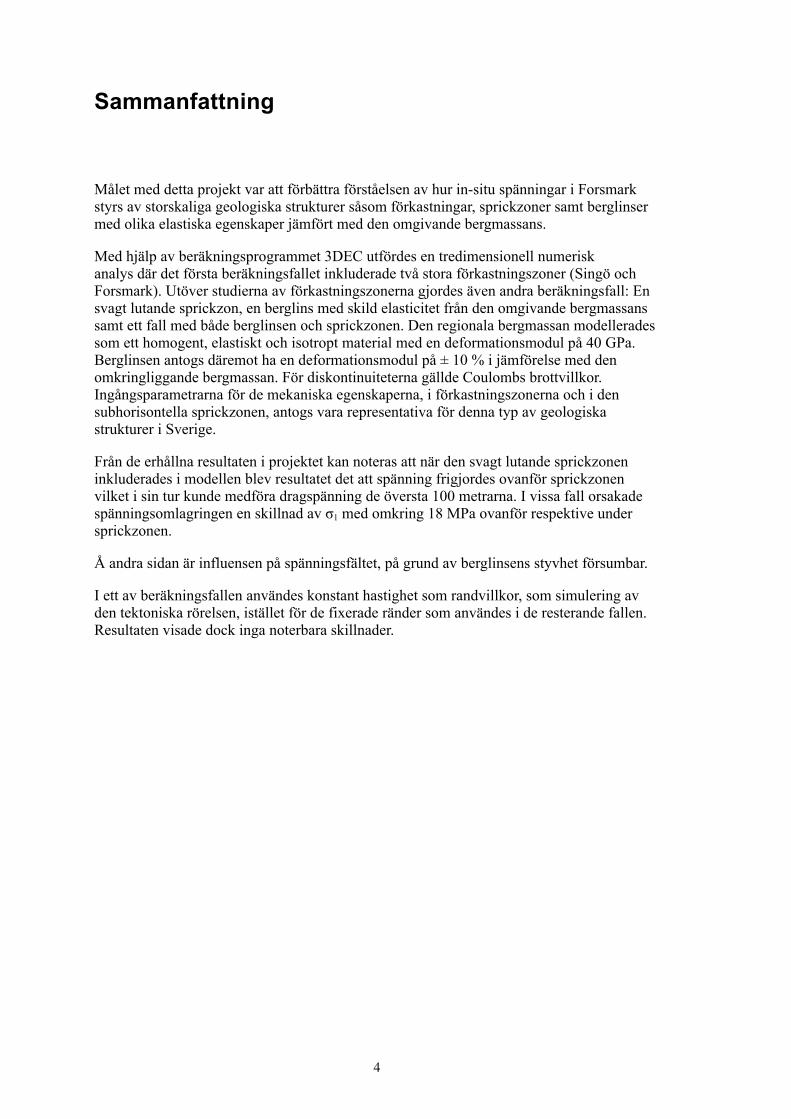
Målet med detta projekt var att förbättra förståelsen av hur in-situ spänningar i Forsmark styrs av storskaliga geologiska strukturer såsom förkastningar, sprickzoner samt berglinser med olika elastiska egenskaper jämfört med den omgivande bergmassans.
Med hjälp av beräkningsprogrammet 3DEC utfördes en tredimensionell numerisk analys där det första beräkningsfallet inkluderade två stora förkastningszoner (Singö och Forsmark). Utöver studierna av förkastningszonerna gjordes även andra beräkningsfall: En svagt lutande sprickzon, en berglins med skild elasticitet från den omgivande bergmassans samt ett fall med både berglinsen och sprickzonen. Den regionala bergmassan modellerades som ett homogent, elastiskt och isotropt material med en deformationsmodul på 40 GPa. Berglinsen antogs däremot ha en deformationsmodul på ± 10 % i jämförelse med den omkringliggande bergmassan. För diskontinuiteterna gällde Coulombs brottvillkor. Ingångsparametrarna för de mekaniska egenskaperna, i förkastningszonerna och i den subhorisontella sprickzonen, antogs vara representativa för denna typ av geologiska strukturer i Sverige.
Från de erhållna resultaten i projektet kan noteras att när den svagt lutande sprickzonen inkluderades i modellen blev resultatet det att spänning frigjordes ovanför sprickzonen vilket i sin tur kunde medföra dragspänning de översta 100 metrarna. I vissa fall orsakade spänningsomlagringen en skillnad av σ1 med omkring 18 MPa ovanför respektive under sprickzonen.
Å andra sidan är influensen på spänningsfältet, på grund av berglinsens styvhet försumbar.
I ett av beräkningsfallen användes konstant hastighet som randvillkor, som simulering av den tektoniska rörelsen, istället för de fixerade ränder som användes i de resterande fallen. Resultaten visade dock inga noterbara skillnader.
5
Contents
1 Objective of the study 7
2 Numerical model 92.1 Geometry of the model 102.2 In-situ and boundary conditions 142.3 Rock mass properties 142.4 Fault zone and fracture zone properties 142.5 Study cases 15
3 Results 173.1 Vertical scan lines DS1, DS2 and DS3 173.2 Horizontal scan lines A, B, C, D, E and F 213.3 Shear displacements 303.4 Displacement vertical cross-section along scan line F 333.5 Principal stress vertical cross-section along scan line F 333.6 Principal stress horizontal cross-section at 450 m depth 42
4 Discussion 45
5 Conclusions 47
References 49
7
1 Objective of the study
The state of stress in an area can be influenced, both in magnitude and orientation, by large-scale features such as faults, fracture zones, and rock lenses with sensibly different elastic properties than the surrounding rock mass. A large number of field, analytical and numerical studies on this matter have been conducted in the last decades /Segall and Pollard, 1980; Pollard and Aydin, 1988; Hyett, 1990; Burgmann and Pollard, 1994; Homberg et al. 1997; Su and Stephansson, 1999; Chester and Chester, 2000/.
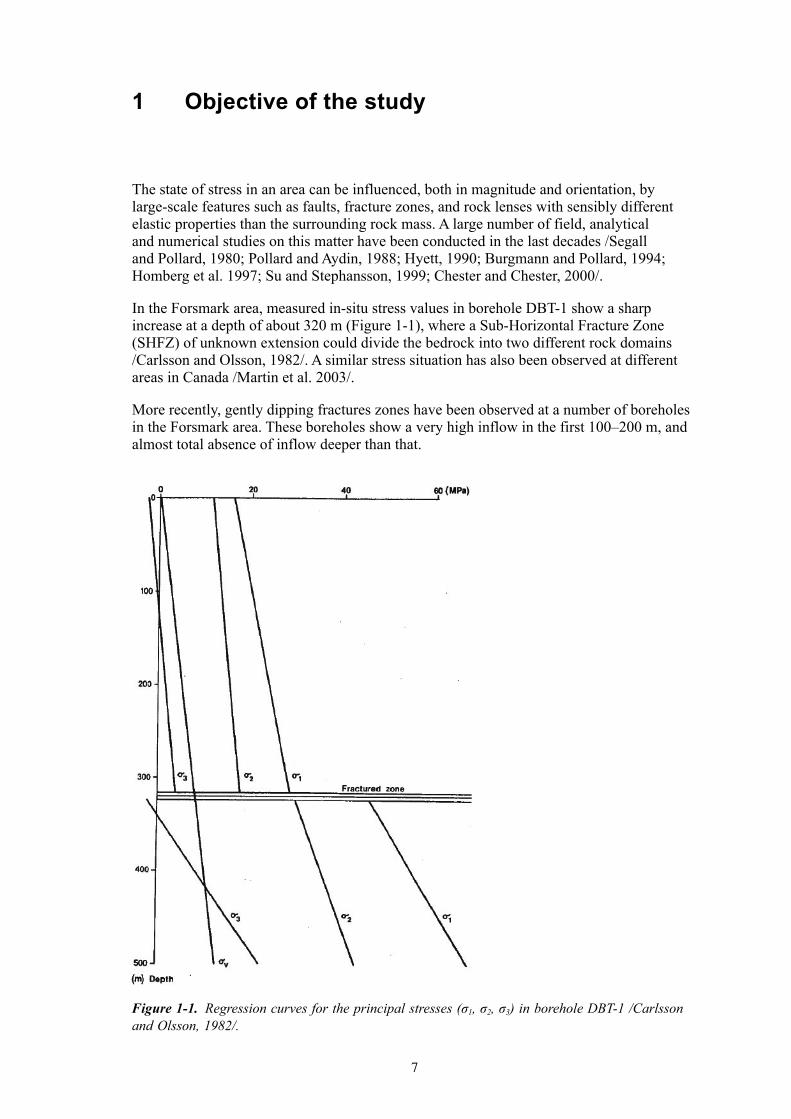
In the Forsmark area, measured in-situ stress values in borehole DBT-1 show a sharp increase at a depth of about 320 m (Figure 1-1), where a Sub-Horizontal Fracture Zone (SHFZ) of unknown extension could divide the bedrock into two different rock domains /Carlsson and Olsson, 1982/. A similar stress situation has also been observed at different areas in Canada /Martin et al. 2003/.
More recently, gently dipping fractures zones have been observed at a number of boreholes in the Forsmark area. These boreholes show a very high inflow in the first 100–200 m, and almost total absence of inflow deeper than that.
Figure 1-1. Regression curves for the principal stresses (σ1, σ2, σ3) in borehole DBT-1 /Carlsson and Olsson, 1982/.

8
The first objective of this study is to evaluate, by means of numerical analysis, the possible influence of a SHFZ, with an unknown extension, and a rock lens with different elastic properties than the surrounding rock mass, on the state of stress in the Forsmark area. It was also intended to study the possible stress concentration in the rock lens due to the geometry of the two fault zones included in the study (Singö fault and Forsmark fault), located on each side of the rock lens.

9
2 Numerical model
This project was initiated at an early stage of the site description model of the Forsmark area – version 1.2 /SKB, 2005/. For this reason, it was considered important to identify the aspects of the geological model that could have the most significant effect on the state of stress at the Forsmark site. Therefore, based on the information contained in the preliminary site description of the Forsmark area – version 1.1 /SKB, 2004/, a numerical model was set up for the analysis of the possible distribution of the stress state at the Forsmark site.
The following assumptions were considered when creating the numerical model:• Two main fault zones have been considered, Singö fault (ZFMNW0001) and Forsmark
fault (ZFMNW0004).– The Forsmark fault, to the west of the study area (Figure 2-1), is very straight
according to airborne geophysical results.– The Singö fault, to the east of the study area (Figure 2-1), is more complex, with
the presence of splays. According to airborne geophysics /SKB, 2000/, it has a more north-ward trend north of the regional model volume, and a more east-ward trend south of the regional model volume. This has been simplified with the curvature of the Singö fault shown in Figure 2-1.
Figure 2-1. Geometrical model of Forsmark area.

10
• The sub-horizontal fracture zone (SHFZ) considered (ZFMNE00A2 /SKB, 2005/), is assumed to have a dip angle of 15°, be continuous for the whole 1 km deep study domain and extend from the Singö fault to the Forsmark fault, but not beyond them. Other sub-horizontal fracture zones are known in the area. These are believed to be smaller than the major SHFZ in the model, and therefore neglected.
• Sub-vertical fracture zones trending NE are also neglected in the model because they are believed to have a minor influence on the current state of stress.
The three-dimensional distinct element code 3DEC, /Itasca, 2003/ was used to perform the numerical simulations. This code is suited to simulate the behavior of rock masses containing multiple, intersecting discontinuities.
2.1 Geometry of the modelThe extension of the model covers an area of 54 km × 49 km in which there is a far field rock mass boundary 8 km thick on each side to diminish the boundary effects. The two main fault zones that have been considered, Singö fault and Forsmark fault, can be seen in Figure 2-1.
A rock lens with different elastic properties is included in some of the simulations to analyze the influence of rock mass heterogeneity on the stress field. The rock lens consists of the orange and the dark blue parts in the center of the model (Figure 2-1).
On Figure 2-2 we can see the numerical model with reference to the coordinate system at Forsmark site according to the Figure 5-13 of the preliminary site description of the Forsmark area – version 1.1 /SKB, 2004/. A rock mass lower boundary of 4 km thickness has been included under the 1 km study domain to diminish the boundary effects.
In Figure 2-3 we can see a close up of the rock lens which, in some of the simulations is divided by a sub-horizontal fracture zone dipping 15° in two different rock masses with different Young’s moduli (10% higher and 10% lower than the surrounding rock mass deformation modulus, E0).
In Figure 2-4 we can see a close-up of the Forsmark model and the scan lines selected to monitor the in-situ stress. DS1, DS2 and DS3 stand for drilling site 1, drilling site 2 and drilling site 3 respectively, as referred to in the preliminary site description of the Forsmark area – version 1.1 /SKB, 2004/. This scan lines are vertical and reach down to a depth of 900 m. DS1 does not intersect the sub-horizontal fracture zone, while DS2 and DS3 intersect it at a depth of 415 m and 785 m respectively.

11
Figure 2-2. Geometrical model of Forsmark area with local and global coordinates.
Figure 2-3. Geometrical model with rock lens and sub-horizontal fracture zone.

12
Scan lines A, B, C, D and E are horizontal and they run through both major fault zones and the rock lens at a depth of 500 m. Scan line F is also horizontal and runs through the rock lens and the sub-horizontal fracture zone at a depth of 500 m.
In Figure 2-5 we can see the zoning of the model. The center part has a maximum zone length of 100 m down to a depth of 1,000 m. Surrounding this fine zoning volume there is another volume of maximum zoning length 250 m from a depth of 1,000 m to a depth of 2,000 m. The rest of the model surrounding these two finer zoning volumes has a maximum zone length of 1,000 m.
Figure 2-4. Forsmark geometrical model showing the position of scan lines.

13
Figure 2-5. Zoning of the numerical model (upper figure) and closer zoom of the finer zoning area (lower figure).
14
2.2 In-situ and boundary conditionsThe in-situ and boundary conditions considered in the model are as follows:• Hydrostatic water pore pressure in the discontinuities.• In-situ stress from the preliminary site description of the Forsmark area – version 1.1
/SKB, 2004/: σ1 trend 134º plunge 0º.
• Lateral and bottom boundaries are no-displacement boundaries.• Upper boundary, coinciding with ground surface, is a boundary with no restraint.
An additional case was modeled to consider the effect of tectonic forces. The in-situ and boundary conditions for this specific case are described in detail in Section 2.5 (Table 2-3).
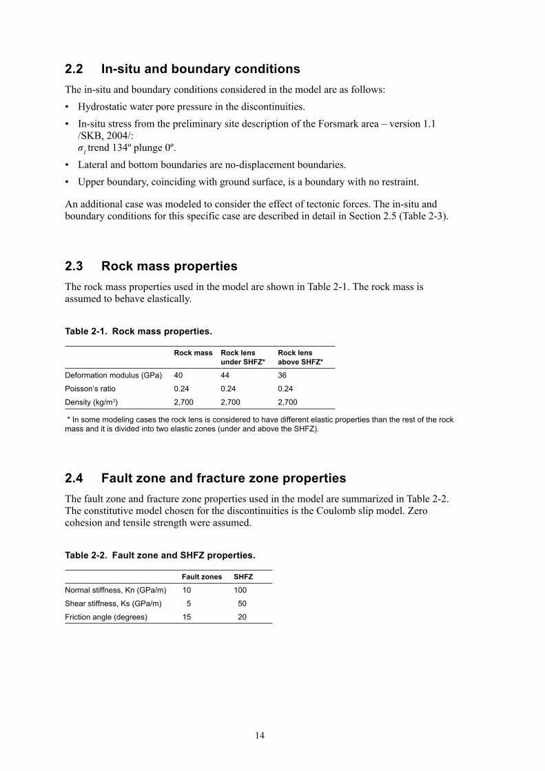
2.3 Rock mass propertiesThe rock mass properties used in the model are shown in Table 2-1. The rock mass is assumed to behave elastically.
Table 2-1. Rock mass properties.
Rock mass Rock lens under SHFZ*
Rock lens above SHFZ*
Deformation modulus (GPa) 40 44 36
Poisson’s ratio 0.24 0.24 0.24
Density (kg/m3) 2,700 2,700 2,700
* In some modeling cases the rock lens is considered to have different elastic properties than the rest of the rock mass and it is divided into two elastic zones (under and above the SHFZ).
2.4 Fault zone and fracture zone propertiesThe fault zone and fracture zone properties used in the model are summarized in Table 2-2. The constitutive model chosen for the discontinuities is the Coulomb slip model. Zero cohesion and tensile strength were assumed.
Table 2-2. Fault zone and SHFZ properties.
Fault zones SHFZ
Normal stiffness, Kn (GPa/m) 10 100
Shear stiffness, Ks (GPa/m) 5 50
Friction angle (degrees) 15 20
15
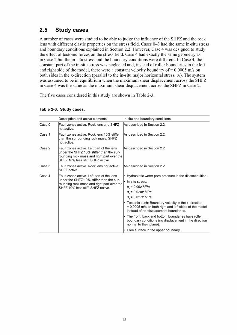
2.5 Study casesA number of cases were studied to be able to judge the influence of the SHFZ and the rock lens with different elastic properties on the stress field. Cases 0–3 had the same in-situ stress and boundary conditions explained in Section 2.2. However, Case 4 was designed to study the effect of tectonic forces on the stress field. Case 4 had exactly the same geometry as in Case 2 but the in-situ stress and the boundary conditions were different. In Case 4, the constant part of the in-situ stress was neglected and, instead of roller boundaries in the left and right side of the model, there were a constant velocity boundary of = 0.0005 m/s on both sides in the x-direction (parallel to the in-situ major horizontal stress, σ1). The system was assumed to be in equilibrium when the maximum shear displacement across the SHFZ in Case 4 was the same as the maximum shear displacement across the SHFZ in Case 2.
The five cases considered in this study are shown in Table 2-3.
Table 2-3. Study cases.
Description and active elements In-situ and boundary conditions
Case 0 Fault zones active. Rock lens and SHFZ not active.
As described in Section 2.2.
Case 1 Fault zones active. Rock lens 10% stiffer than the surrounding rock mass. SHFZ not active.
As described in Section 2.2.
Case 2 Fault zones active. Left part of the lens under the SHFZ 10% stiffer than the sur-rounding rock mass and right part over the SHFZ 10% less stiff. SHFZ active.
As described in Section 2.2.
Case 3 Fault zones active. Rock lens not active. SHFZ active.
As described in Section 2.2.
Case 4 Fault zones active. Left part of the lens under the SHFZ 10% stiffer than the sur-rounding rock mass and right part over the SHFZ 10% less stiff. SHFZ active.
• Hydrostatic water pore pressure in the discontinuities.
• In-situ stress: σ1 = 0.09z MPa σ1 = 0.028z MPa σ1 = 0.027z MPa
• Tectonic push: Boundary velocity in the x-direction = 0.0005 m/s on both right and left sides of the model instead of no-displacement boundaries.
• The front, back and bottom boundaries have roller boundary conditions (no displacement in the direction normal to their plane).
• Free surface in the upper boundary.
17
3 Results
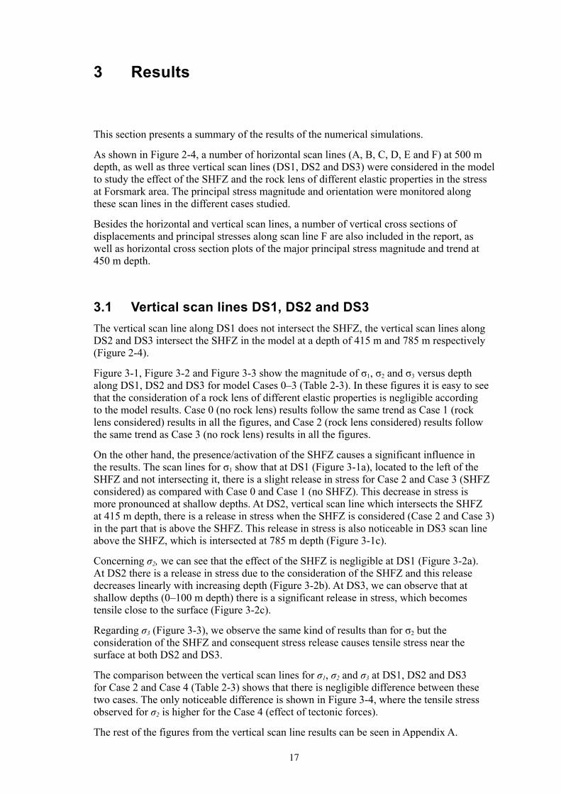
This section presents a summary of the results of the numerical simulations.
As shown in Figure 2-4, a number of horizontal scan lines (A, B, C, D, E and F) at 500 m depth, as well as three vertical scan lines (DS1, DS2 and DS3) were considered in the model to study the effect of the SHFZ and the rock lens of different elastic properties in the stress at Forsmark area. The principal stress magnitude and orientation were monitored along these scan lines in the different cases studied.
Besides the horizontal and vertical scan lines, a number of vertical cross sections of displacements and principal stresses along scan line F are also included in the report, as well as horizontal cross section plots of the major principal stress magnitude and trend at 450 m depth.
3.1 Vertical scan lines DS1, DS2 and DS3The vertical scan line along DS1 does not intersect the SHFZ, the vertical scan lines along DS2 and DS3 intersect the SHFZ in the model at a depth of 415 m and 785 m respectively (Figure 2-4).
Figure 3-1, Figure 3-2 and Figure 3-3 show the magnitude of σ1, σ2 and σ3 versus depth along DS1, DS2 and DS3 for model Cases 0–3 (Table 2-3). In these figures it is easy to see that the consideration of a rock lens of different elastic properties is negligible according to the model results. Case 0 (no rock lens) results follow the same trend as Case 1 (rock lens considered) results in all the figures, and Case 2 (rock lens considered) results follow the same trend as Case 3 (no rock lens) results in all the figures.
On the other hand, the presence/activation of the SHFZ causes a significant influence in the results. The scan lines for σ1 show that at DS1 (Figure 3-1a), located to the left of the SHFZ and not intersecting it, there is a slight release in stress for Case 2 and Case 3 (SHFZ considered) as compared with Case 0 and Case 1 (no SHFZ). This decrease in stress is more pronounced at shallow depths. At DS2, vertical scan line which intersects the SHFZ at 415 m depth, there is a release in stress when the SHFZ is considered (Case 2 and Case 3) in the part that is above the SHFZ. This release in stress is also noticeable in DS3 scan line above the SHFZ, which is intersected at 785 m depth (Figure 3-1c).
Concerning σ2, we can see that the effect of the SHFZ is negligible at DS1 (Figure 3-2a). At DS2 there is a release in stress due to the consideration of the SHFZ and this release decreases linearly with increasing depth (Figure 3-2b). At DS3, we can observe that at shallow depths (0–100 m depth) there is a significant release in stress, which becomes tensile close to the surface (Figure 3-2c).
Regarding σ3 (Figure 3-3), we observe the same kind of results than for σ2 but the consideration of the SHFZ and consequent stress release causes tensile stress near the surface at both DS2 and DS3.
The comparison between the vertical scan lines for σ1, σ2 and σ3 at DS1, DS2 and DS3 for Case 2 and Case 4 (Table 2-3) shows that there is negligible difference between these two cases. The only noticeable difference is shown in Figure 3-4, where the tensile stress observed for σ2 is higher for the Case 4 (effect of tectonic forces).
The rest of the figures from the vertical scan line results can be seen in Appendix A.

18
Figure 3-1. σ1 vs. depth for Cases 0–3 at: a) DS1 b) DS2 and c) DS3.
Sigma1 scanline at DS1
-1,000
-900
-800
-700
-600
-500
-400
-300
-200
-100
0-1.0E+08 -8.0E+07 -6.0E+07 -4.0E+07 -2.0E+07 0.0E+00
Stress (Pa)
Case0Case1Case2Case3
a)
Sigma1 scanline at DS2
-1,000
-900
-800
-700
-600
-500
-400
-300
-200
-100
0-1.0E+08 -8.0E+07 -6.0E+07 -4.0E+07 -2.0E+07 0.0E+00
Stress (Pa)
Case0Case1Case2Case3
b)
Sigma1 scanline at DS3
-1,000
-900
-800
-700
-600
-500
-400
-300
-200
-100
0-1.0E+08 -8.0E+07 -6.0E+07 -4.0E+07 -2.0E+07 0.0E+00
Stress (Pa)
Case0Case1Case2Case3
c)
Dep
th (
m)
Dep
th (
m)
Dep
th (
m)

19
Figure 3-2. σ2 vs. depth for Cases 0–3 at: a) DS1 b) DS2 and c) DS3.
Sigma2 scanline at DS1
-1,000
-900
-800
-700
-600
-500
-400
-300
-200
-100
0-3.0E+07 -2.5E+07 -2.0E+07 -1.5E+07 -1.0E+07 -5.0E+06 0.0E+00
Stress (Pa)
Case0Case1Case2Case3
a)
Sigma2 scanline at DS2
-1,000
-900
-800
-700
-600
-500
-400
-300
-200
-100
0-3.0E+07 -2.5E+07 -2.0E+07 -1.5E+07 -1.0E+07 -5.0E+06 0.0E+00
Stress (Pa)
Case0Case1Case2Case3
b)
Sigma2 scanline at DS3
-1,000
-900
-800
-700
-600
-500
-400
-300
-200
-100
0-4.0E+07 -3.0E+07 -2.0E+07 -1.0E+07 0.0E+00 1.0E+07
Stress (Pa)
Case0Case1Case2Case3
c)
Dep
th (
m)
Dep
th (
m)
Dep
th (
m)

20
Figure 3-3. σ3 vs. depth for Cases 0–3 at: a) DS1 b) DS2 and c) DS3.
Sigma3 scanline at DS1
-1,000
-900
-800
-700
-600
-500
-400
-300
-200
-100
0-3.0E+07 -2.5E+07 -2.0E+07 -1.5E+07 -1.0E+07 -5.0E+06 0.0E+00
Stress (Pa)
Case0Case1Case2Case3
a)
Sigma3 scanline at DS2
-1,000
-900
-800
-700
-600
-500
-400
-300
-200
-100
0-3.0E+07 -2.0E+07 -1.0E+07 0.0E+00 1.0E+07
Stress (Pa)
Case0Case1Case2Case3
b)
Sigma3 scanline at DS3
-1000
-900
-800
-700
-600
-500
-400
-300
-200
-100
0-3.0E+07 -2.0E+07 -1.0E+07 0.0E+00 1.0E+07
Stress (Pa)
Case0Case1Case2Case3
c)
Dep
th (
m)
Dep
th (
m)
Dep
th (
m)

21
Figure 3-4. σ2 vs. depth for Cases 2 and 4 at DS3.
Sigma2 scanline at DS3
-1,000
-900
-800
-700
-600
-500
-400
-300
-200
-100
0
-3.0E+07 -2.0E+07 -1.0E+07 0.0E+00 1.0E+07
Stress (Pa)
)m(
htp
eD
Case2
Case4
3.2 Horizontal scan lines A, B, C, D, E and FThe horizontal scan lines are all defined at 500 m depth. However, the principal stresses in 3DEC are calculated in each zone centroid and, due to the geometrical complexity of the zoning, some of the zone centroids are not located at 500 m depth. For this reason the horizontal stress scan lines include the principal stress magnitude and orientation at 500 ± 30 m depth. This causes fluctuation in the stress values presented in the figures of the horizontal scan lines. For the purpose of this study, which is the evaluation of the influence of the SHFZ and the rock lens, this grid-dependent variability in depth of the monitoring points along the scan lines is judged to have no influence, as we are interested in the relative difference between the modeling cases.
Scan lines A, B, C, D and E are all parallel to the outcrop of the SHFZ (Figure 2-4). Scan line A is located at 500 m depth and at 3 km to the left from the outcrop of the SHFZ. Scan line B is 1 km to the left of the SHFZ outcrop. Scan line C is 200 m under the SHFZ and 1 km to the SE of the fracture zone outcrop. Scan line D is located 320 m over the SHFZ and 3 km to the SE of its outcrop. And scan line D is 5 km to the SE of the outcrop of the SHFZ. Scan line F, at 500 m depth, is perpendicular to the SHFZ outcrop and intersects it at 30,500 m along the x-axis.
In Figure 3-5 and Figure 3-6 we can see the variation in σ1 magnitude along scan lines A, B, C, D and E for modelling Cases 0–3. A trendline curve (polynomial regression) has been added in these figures to give a clearer idea of the relative difference between the cases analyzed. The trendline decreases the effect of the fluctuation caused by the zone centroid spatial variability.

22
Figure 3-5. σ1 magnitude along horizontal scan lines A and B at 500 m depth for Cases 0–3 together with trendlines (polynomial regression) for Case 0 and 2.
Sigma1 scanline A
-5.5E+07
-5.0E+07
-4.5E+07
-4.0E+07
-3.5E+0718,000 20,000 22,000 24,000 26,000
Z axis (m)
Case0Case1Case2Case3Trendline (Case0)Trendline (Case2)
Sigma1 scanline B
-5.5E+07
-5.0E+07
-4.5E+07
-4.0E+07
-3.5E+0718,000 20,000 22,000 24,000 26,000
Z axis (m)
Case0Case1Case2Case3Trendline (Case0)Trendline (Case2)
FF SF SF : Singö Fault
FF : Forsmark Fault
FF SF
Str
ess
(Pa)
Str
ess
(Pa)
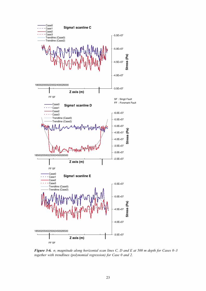
In these figures we see that the consideration of a rock lens of different elastic properties is negligible according to the model results. This was also observed in the vertical scan lines results.
The gradual decrease in stress in the area between the Forsmark fault zone and the Singö fault zone when the SHFZ is considered (Case 2 and Case 3) may be observed from scan lines A to D, to increase again in scan line E. The maximum decrease in σ1 magnitude (about 18 MPa less in the area between the fault zones when the SHFZ is considered) is observed along scan line D (Figure 3-6).
23
Figure 3-6. σ1 magnitude along horizontal scan lines C, D and E at 500 m depth for Cases 0–3 together with trendlines (polynomial regression) for Case 0 and 2.
Sigma1 scanline C
-5.5E+07
-5.0E+07
-4.5E+07
-4.0E+07
-3.5E+071800020000220002400026000
Z axis (m)
Case0Case1Case2Case3Trendline (Case0)Trendline (Case2)
Sigma1 scanline D
-6.0E+07
-5.5E+07
-5.0E+07
-4.5E+07
-4.0E+07
-3.5E+07
-3.0E+07
-2.5E+071850020500225002450026500
Z axis (m)
Case0Case1Case2Case3Trendline (Case0)Trendline (Case2)
Sigma1 scanline E
-5.5E+07
-5.0E+07
-4.5E+07
-4.0E+07
-3.5E+071850020500225002450026500
Z axis (m)
Case0Case1Case2Case3Trendline (Case0)Trendline (Case2)
SF : Singö Fault
FF : Forsmark Fault
FF SF
FF SF
FF SF
Str
ess
(Pa)
Str
ess
(Pa)
Str
ess
(Pa)

24
In Figure 3-7 we can see the change in σ1 trend along scan lines A, B and E. The cero value on the y-axis in Figure 3-7 refers to the situation where σ1 has the same trend as the applied in-situ σ1 (134°). A positive or negative value along the y-axis means the trend of σ1 is larger or smaller than 134° respectively. It is very noticeable the different influence of the Forsmark fault zone and the Singö fault zone due to the different relative orientation of these two fault zones (notice the curvature of the Singö fault in Figure 2-1) with respect to the in-situ stress applied in the model.
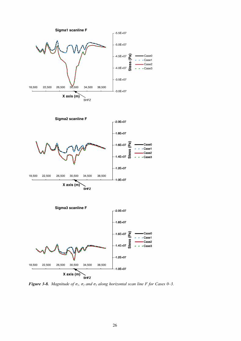
Figure 3-8 shows the change in the magnitude of σ1, σ2 and σ3 along scan line F for modelling Cases 0–3. As can be seen, the decrease in σ1 magnitude due to the SHFZ reaches a maximum of about 18 MPa where scan line F passes through the fracture zone (30,500 m in the x-axis). The area of influence of the SHFZ in the magnitude of σ1 is roughly 8 km to the SE and to the left of the intersection of the scan line F with the fracture zone.
The decrease in the magnitude of σ2 and σ3 when considering the SHFZ follows the same tendency as for the case of σ1. The maximum difference in the magnitudes of the stress is always at the intersection with the fracture zone (30,500 m in the x-axis).
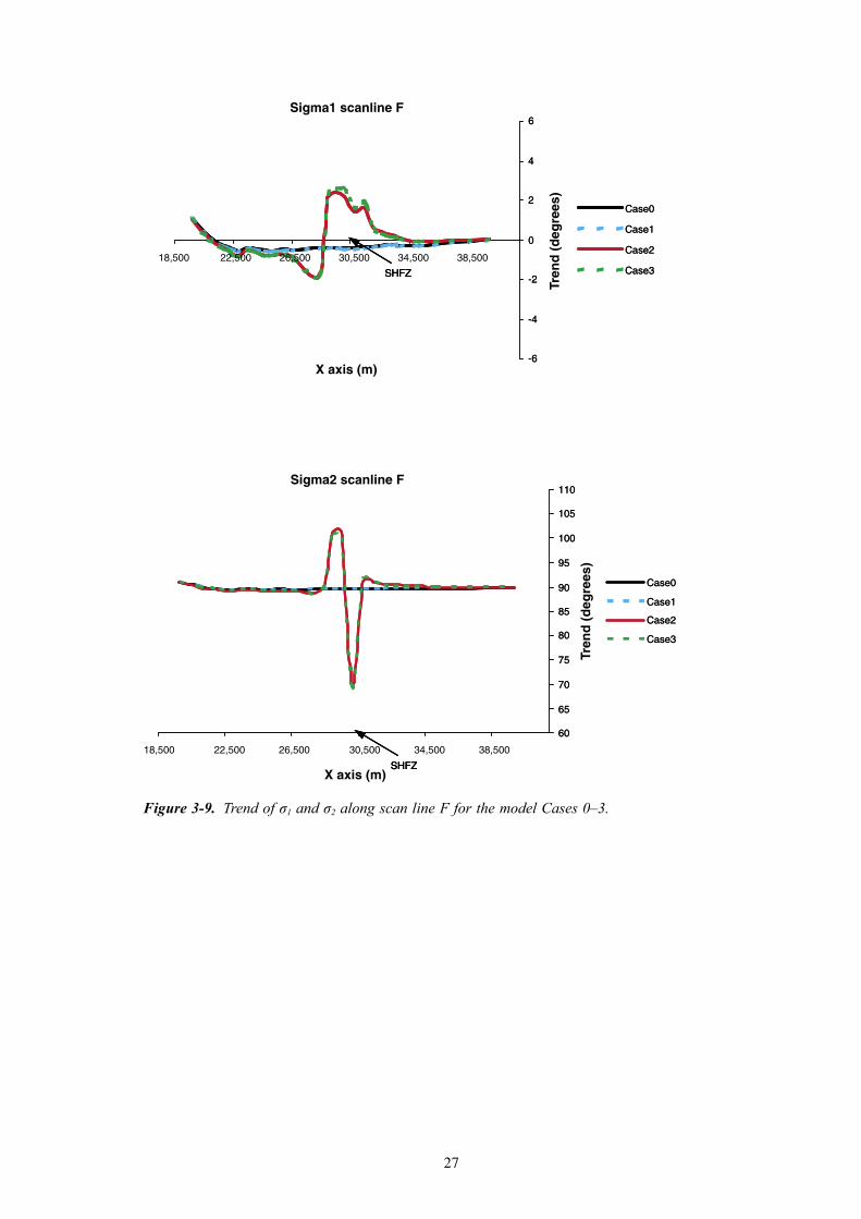
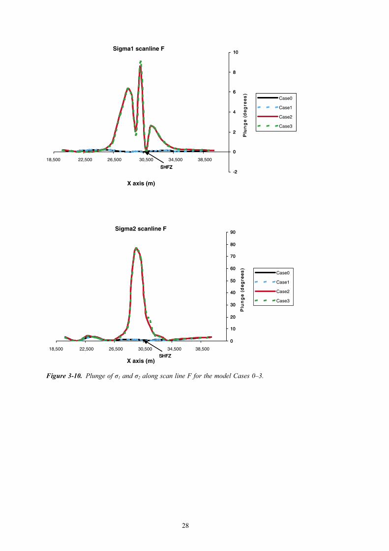
In Figure 3-9 and Figure 3-10 we can see the trend and plunge of σ1 and σ2 along scan line F for the model Cases 0–3. The cero value on the y-axis in the upper plot in Figure 3-7 refers to the situation where σ1 has the same trend as the applied in-situ σ1 (134°). A positive or negative value along the y-axis means the trend of σ1 is larger or smaller than 134° respectively. The same applies to the lower plot in Figure 3-7, where the value 90° applies to the situation where σ2 has the same trend as the applied in-situ σ2 (224°). Likewise, the cero value on the y-axis in Figure 3-10 refers to the situation where σ1 and σ2 have the same plunge as in the applied in-situ stress (0°).
In these figures (Figure 3-9 and Figure 3-10), the influence of the SHFZ can be easily noticed. We can see also that the influence of the SHFZ on the plunge is higher than the influence on the trend of σ1 and σ2.
The difference between the magnitude of σ1, σ2 and σ3 along scan line F for model Case 2 and model Case 4 (tectonic loading) can be seen in Figure 3-11. The general tendency along scan line F is the same. However, while for Case 2 the magnitude of σ1 is always lower than for Case 4, the magnitudes of σ2 and σ3 are higher for Case 2 than for Case 4. The difference, nonetheless, is insignificant.

25
Figure 3-7. σ1 trend along horizontal scan lines A, B and E at 500 m depth for Cases 0–3.
Sigma1 scanline A
-7
-5
-3
-1
1
3
5
18,000 20,000 22,000 24,000 26,000
Z axis (m)
Case0
Case1
Case2
Case3
Sigma1 scanline B
-9
-7
-5
-3
-1
1
3
5
18,000 20,000 22,000 24,000 26,000
Z axis (m)
Case0
Case1
Case2
Case3
Sigma1 scanline E
-15
-12
-9
-6
-3
0
3
6
9
18,500 20,500 22,500 24,500 26,500
Z axis (m)
Case0
Case1
Case2
Case3
SF
SF : Singö Fault
FF : Forsmark Fault
FF
FF SF
SFFF
Tren
d d
egre
eTr
end
deg
ree
Tren
d d
egre
e
26
Figure 3-8. Magnitude of σ1, σ2 and σ3 along horizontal scan line F for Cases 0–3.
Sigma1 scanline F-5.5E+07
-5.0E+07
-4.5E+07
-4.0E+07
-3.5E+07
-3.0E+0718,500 22,500 26,500 30,500 34,500 38,500
X axis (m)
Case0
Case1
Case2
Case3
SHFZ
-2.0E+07
-1.8E+07
-1.6E+07
-1.4E+07
-1.2E+07
-1.0E+0718,500 22,500 26,500 30,500 34,500 38,500
X axis (m)
Case0
Case1
Case2
Case3
SHFZ
Sigma2 scanline F-2.0E+07
-1.8E+07
-1.6E+07
-1.4E+07
-1.2E+07
-1.0E+07
Case0
Case1
Case2
Case3
SHFZSHFZ
-2.0E+07
-1.8E+07
-1.6E+07
-1.4E+07
-1.2E+07
-1.0E+0718,500 22,500 26,500 30,500 34,500 38,500
Case0
Case1
Case2
Case3
SHFZ
Sigma3 scanline F-2.0E+07
-1.8E+07
-1.6E+07
-1.4E+07
-1.2E+07
-1.0E+07
X axis (m)
Case0
Case1
Case2
Case3
SHFZSHFZ
Ste
ss (
Pa)
Ste
ss (
Pa)
Ste
ss (
Pa)
27
Figure 3-9. Trend of σ1 and σ2 along scan line F for the model Cases 0–3.
Sigma1 scanline F
-6
-4
-2
0
2
4
6
X axis (m)
Case0
Case1
Case2
Case3SHFZ
-6
-4
-2
0
2
4
6
Case0
Case1
Case2
Case3SHFZSHFZ
Sigma2 scanline F
60
65
70
75
80
85
90
95
100
105
110
18,500 22,500 26,500 30,500 34,500 38,500
X axis (m)
Case0
Case1
Case2
Case3
SHFZ
60
65
70
75
80
85
90
95
100
105
110
Case0
Case1
Case2
Case3
SHFZSHFZ
18,500 22,500 26,500 30,500 34,500 38,500
Tren
d (
deg
rees
)
Tren
d (
deg
rees
)
28
Figure 3-10. Plunge of σ1 and σ2 along scan line F for the model Cases 0–3.
Sigma1 scanline F
-2
0
2
4
6
8
10
18,500 22,500 26,500 30,500 34,500 38,500
X axis (m)
)s
eer
ge
d( e
gn
ulP
Case0
Case1
Case2
Case3
SHFZ-2
0
2
4
6
8
10
)s
eer
ge
d( e
gn
ulP
Case0
Case1
Case2
Case3
SHFZSHFZ
Sigma2 scanline F
0
10
20
30
40
50
60
70
80
90
18,500 22,500 26,500 30,500 34,500 38,500
X axis (m)
)s
eer
ge
d( e
gn
ulP
Case0
Case1
Case2
Case3
SHFZ
0
10
20
30
40
50
60
70
80
90
)s
eer
ge
d( e
gn
ulP
Case0
Case1
Case2
Case3
SHFZSHFZ

29
Figure 3-11. Magnitude of σ1, σ2 and σ3 along horizontal scan lines F for model Cases 2 and 4.
Sigma1 scanline F-5.5E+07
-5.0E+07
-4.5E+07
-4.0E+07
-3.5E+07
-3.0E+07
18,500 22,500 26,500 30,500 34,500 38,500
X axis (m)
Case2
Case4
SHFZ
-5.5E+07
-5.0E+07
-4.5E+07
-4.0E+07
-3.5E+07
-3.0E+07
Case2
Case4
SHFZSHFZ
Sigma2 scanline F-2.0E+07
-1.8E+07
-1.6E+07
-1.4E+07
-1.2E+07
-1.0E+07
18,500 22,500 26,500 30,500 34,500 38,500
X axis (m)
Case2
Case4
SHFZ
-2.0E+07
-1.8E+07
-1.6E+07
-1.4E+07
-1.2E+07
-1.0E+07
Case2
Case4
SHFZSHFZ
Sigma3 scanline F-1.6E+07
-1.5E+07
-1.4E+07
-1.3E+07
-1.2E+07
-1.1E+07
-1.0E+07
185002250026500305003450038500
X axis (m)
)aP( ssert
S
Case2
Case4
SHFZ
-1.6E+07
-1.5E+07
-1.4E+07
-1.3E+07
-1.2E+07
-1.1E+07
-1.0E+07
185002250026500305003450038500
)aP( ssert
S
Case2
Case4
SHFZSHFZ
Str
ess
(Pa)
Str
ess
(Pa)
30
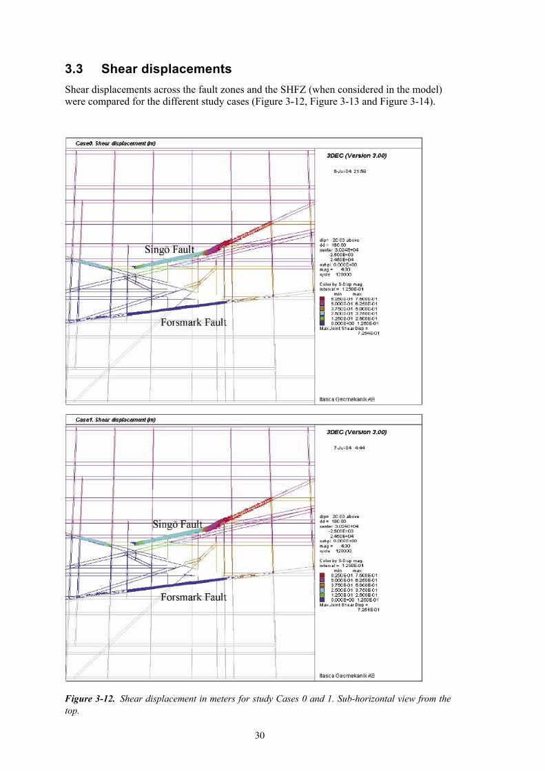
3.3 Shear displacementsShear displacements across the fault zones and the SHFZ (when considered in the model) were compared for the different study cases (Figure 3-12, Figure 3-13 and Figure 3-14).
Figure 3-12. Shear displacement in meters for study Cases 0 and 1. Sub-horizontal view from the top.
31
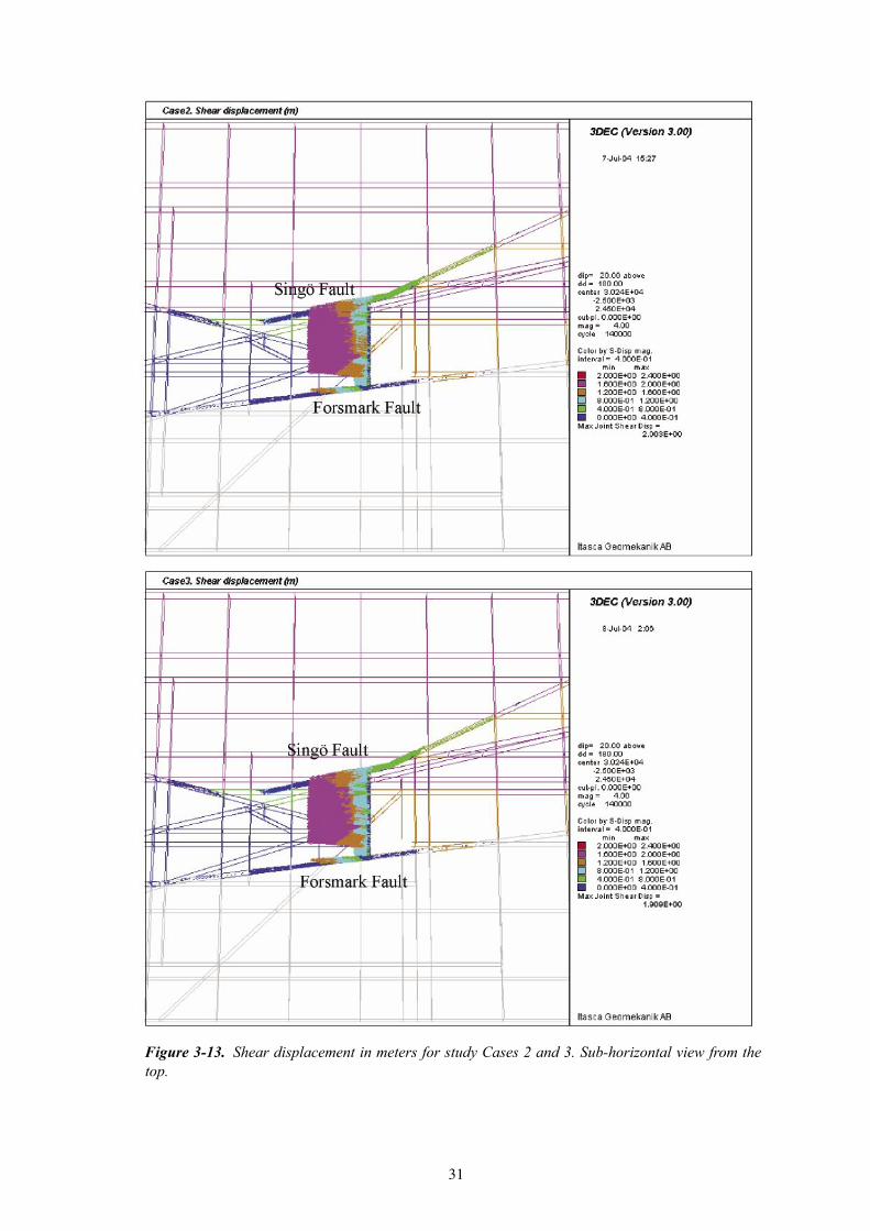
Figure 3-13. Shear displacement in meters for study Cases 2 and 3. Sub-horizontal view from the top.
32
Figure 3-12 shows the shear displacement across the fault zones for Cases 0 and 1 in which no SHFZ is considered. We can see that the shear displacement is much lower across the Forsmark fault due to the low angle between the fault and the regional maximum principal stress. The shear displacement across this fault is less than 12.5 cm. On the other hand, as the Singö fault is curved, some parts of the fault (red colour in Figure 3-12) form a more pronounced angle relative to the regional maximum principal stress and so the shear displacement on those parts is much larger (62.5 to 72.5 cm). As a consequence of this localized large shear displacement, the entire Singö fault is mobilized and the shear displacement is larger across the whole fault than for the Forsmark fault. It is easy to see that the influence of considering a rock lens with 10% difference in deformation modulus (Case 1) has negligible influence in the shear displacement.
In Figure 3-13 we can see the shear displacement when the SHFZ is considered (Case 2 and Case 3). The large shear displacements across the SHFZ reach a maximum value of 2 m near the outcrop of the fracture zone for Case 2 (rock lens of different elastic properties considered). When the rock lens is not considered (Case 3) the maximum shear displacement across the SHFZ decreases to 1.9 m.
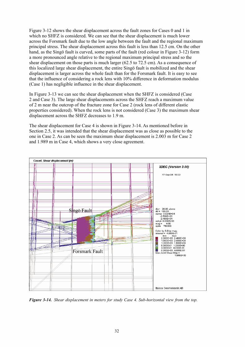
The shear displacement for Case 4 is shown in Figure 3-14. As mentioned before in Section 2.5, it was intended that the shear displacement was as close as possible to the one in Case 2. As can be seen the maximum shear displacement is 2.003 m for Case 2 and 1.989 m in Case 4, which shows a very close agreement.
Figure 3-14. Shear displacement in meters for study Case 4. Sub-horizontal view from the top.

33
3.4 Displacement vertical cross-section along scan line FThis section presents a series of figures of the displacement vectors in a vertical cross-section along scan line F.
In Figure 3-15 we can see the displacement vectors in a vertical cross-section along scan line F for study Case 0 and 1. As can be seen, the effect of introducing a stiffer rock lens without including the SHFZ is negligible in this case.
Figure 3-16 and Figure 3-17 show the displacement vectors over the same cross-section when the SHFZ is considered. While in the area under the fracture the displacement field is similar to the one for Cases 0 and 1, in the area over the fracture we see the large movement towards the ground surface. When considering the rock lens (Case 2) the maximum displacement is larger than without the rock lens included (Case 3).
In Figure 3-18 we see the vertical cross-sectional plot of the displacement vectors along scan line F for Case 4. The influence of the constant velocity boundary conditions is visible in the figure where we can see the different displacement along different areas of the cross-section.
3.5 Principal stress vertical cross-section along scan line FThe figures in this section show vertical cross-section plots of the principal stresses taken at scan line F for the different study cases.
As can be seen in Figure 3-19 the influence of a rock lens of 10% higher deformation modulus is negligible.
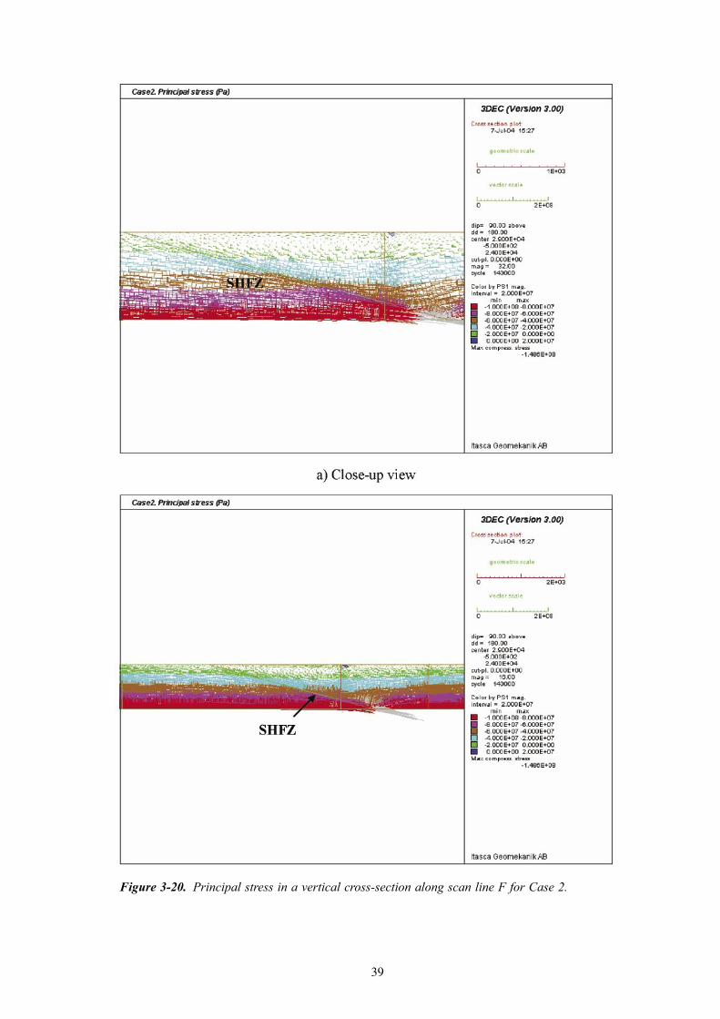
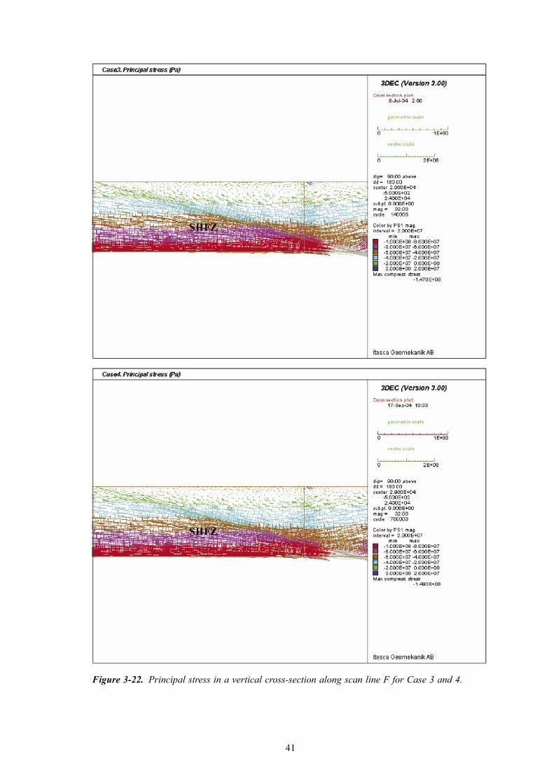
When the SHFZ is included in the analysis (Case 2, Case 3 and Case 4) the stress field in the immediate surrounding of the SHFZ is modified in magnitude and orientation (Figure 3-20, Figure 3-21 and Figure 3-22). It is important to note the release in stress above the fracture zone. Tensile stresses develop near the surface as a consequence of this release in stress (Figure 3-20, Figure 3-21 and Figure 3-22). The presence of tensile stresses in the first 100 m is also observed in the vertical scan lines presented in Section 3.1 (Figure 3-2, Figure 3-3 and Figure 3-4).
As can be seen in Figure 3-21 (Case 2), when the SHFZ is considered there is an increase in the stress under a depth of about 850 m compared to the cases with no SHFZ in Figure 3-19. This way the maximum compressive stress reaches a value of 150 MPa when the SHFZ is considered (possibly caused by stress concentration in the tip of the SHFZ) while, with no SHFZ (Figure 3-19), the maximum compressive stress reaches a value of around 94 MPa at large depth.
The consideration of a rock lens with different elastic properties shows negligible effect in the stress field as shown in preceding results and in Figure 3-20, Figure 3-21 and Figure 3-22.
The comparison between Case 2 and Case 4 (Figure 3-21 and Figure 3-22) shows that the analysis with the tectonic loading at the boundaries does not make any noticeable change. Further study would be needed in this area to be able to achieve more objective conclusions.

34
Figure 3-15. Displacement vectors in a vertical cross-section along scan line F for Case 0 and 1.

35
Figure 3-16. Displacement vectors in a vertical cross-section along scan line F for Case 2.

36
Figure 3-17. Displacement vectors in a vertical cross-section along scan line F for Case 3.

37
Figure 3-18. Displacement vectors in a vertical cross-section along scan line F for Case 4.

38
Figure 3-19. Principal stress in a vertical cross-section along scan line F for Cases 0 and 1.
39
Figure 3-20. Principal stress in a vertical cross-section along scan line F for Case 2.

40
Figure 3-21. Principal stress in a vertical cross-section along scan line F for Case 2 with different stress magnitude ranges.
41
Figure 3-22. Principal stress in a vertical cross-section along scan line F for Case 3 and 4.

42
3.6 Principal stress horizontal cross-section at 450 m depthThis section presents horizontal cross section plots of the major principal stress magnitude and trend at 450 m depth.
In Figure 3-23a, we can see that the effect of the Singö fault on the major principal stress magnitude σ1 is much more pronounced (specially in the eastern part of the Singö fault) than that of the Forsmark fault. This is due to the relative orientation of the faults in relation to the applied regional stress.
When the SHFZ is included in the model (Figure 3-23b), a stress release area is noticeable to the east of the fracture zone. While the regional major principal stress magnitude at 450 m depth is 44.5 MPa, in the de-stressed area values of 24 MPa are reached.
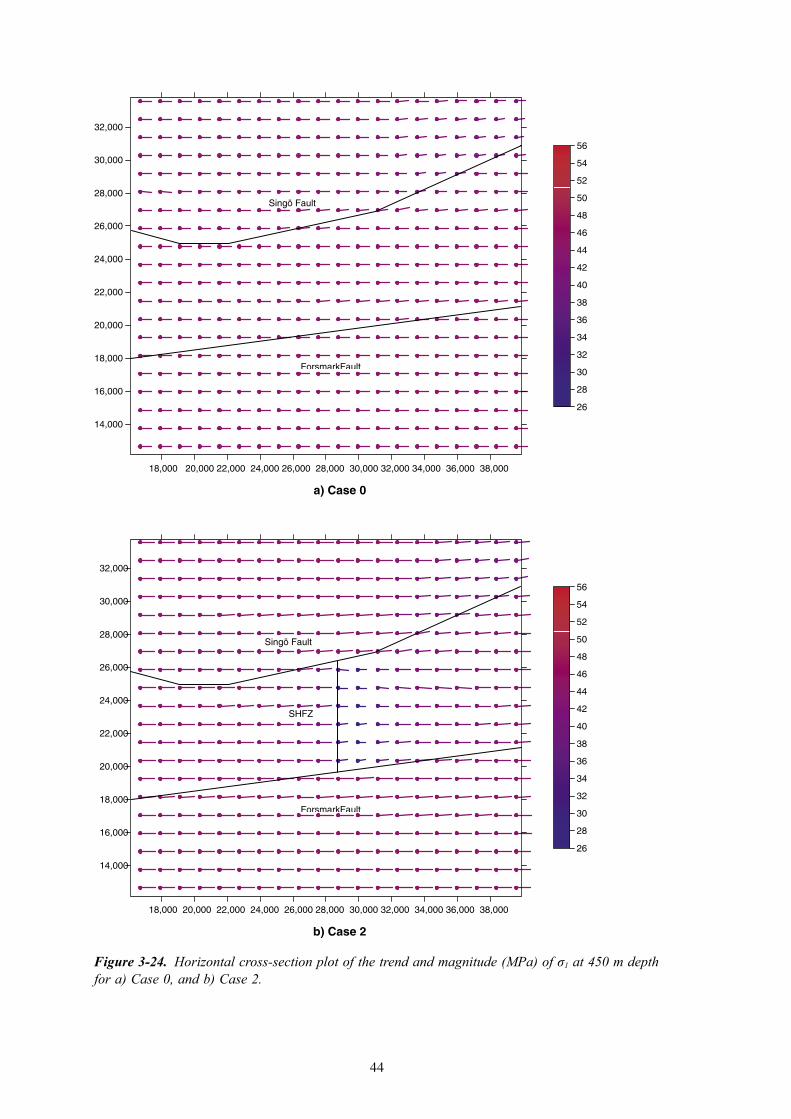
The trend of the major principal stress, σ1, at 450 m depth is shown in Figure 3-24. In Figure 3-24a we can see that the influence on the trend of σ1 of the Singö fault, specially the part on the right of the figure, is much more pronounced than the influence of the Forsmark fault. In this case (Case 0) the maximum deviation from the regional trend of σ1 is 13.8°.
When the SHFZ is included in the model (Figure 3-24b), the trend of σ1 is disturbed also in the vicinity of the fracture zone. In this case (Case 2), the maximum deviation from the regional trend of σ1 is 14.5°.

43
Figure 3-23. Horizontal cross-section plot of the magnitude contours (MPa) of σ1 at 450 m depth for a) Case 0, and b) Case 2.
18,000 20,000 22,000 24,000 26,000 28,000 30,000 32,000 34,000 36,000 38,000
14,000
16,000
18,000
20,000
22,000
24,000
26,000
28,000
30,000
32,000
-56
-54
-52
-50
-48
-46
-44
-42
-40
-38
-36
-34
-32
-30
-28
-26
a) Case 0
18,000 20,000 22,000 24,000 26,000 28,000 30,000 32,000 34,000 36,000 38,000
14,000
16,000
18,000
20,000
22,000
24,000
26,000
28,000
30,000
32,000
-56
-54
-52
-50
-48
-46
-44
-42
-40
-38
-36
-34
-32
-30
-28
-26
b) Case 2
ForsmarkFault
SHFZ
Singö Fault
Singö Fault
ForsmarkFault
44
Figure 3-24. Horizontal cross-section plot of the trend and magnitude (MPa) of σ1 at 450 m depth for a) Case 0, and b) Case 2.
18,000 20,000 22,000 24,000 26,000 28,000 30,000 32,000 34,000 36,000 38,000
14,000
16,000
18,000
20,000
22,000
24,000
26,000
28,000
30,000
32,000
26
28
30
32
34
36
38
40
42
44
46
48
50
52
54
56
a) Case 0
18,000 20,000 22,000 24,000 26,000 28,000 30,000 32,000 34,000 36,000 38,000
14,000
16,000
18,000
20,000
22,000
24,000
26,000
28,000
30,000
32,000
26
28
30
32
34
36
38
40
42
44
46
48
50
52
54
56
b) Case 2
Singö Fault
Singö Fault
ForsmarkFault
SHFZ
ForsmarkFault

45
4 Discussion
The purpose of this section is to highlight several aspects that had an impact on this modeling study and should be taken into account when reading the conclusions.
In the time when this project was carried out there were a number of uncertainties concerning the definition of the conceptual model, mainly due to shortage of input data from the site description model of the Forsmark area – version 1.1 /SKB, 2004/. Much of this input data is already provided in version 1.2 /SKB, 2005/, so that future studies can benefit from it. The main sources of uncertainty identified in the model are:• Extension, location and orientation of the SHFZ. In the conceptual model it is assumed
that the SHFZ extends from the Singö fault to the Forsmark fault, not continuing beyond those two faults. It is further assumed that the fracture zone is continuous until 1,000 m depth. (See Figure 2-1 and Figure 2-3). The dip of the SHFZ is assumed to be 15°. When more data is available regarding the actual geometry of the SHFZ, further analysis would be necessary to judge the influence of these assumptions.
• The input values used for the mechanical properties of the Fault zones and the SHFZ are assumed to be representative of this kind of geological features in Sweden, as no specific data was provided. Early work by /Zoback and Healy, 1984; Hyett, 1990/, and more recent studies by /Homberg et al. 1997/ and by /Su and Stephansson, 1999/ between others, show that one of the most relevant parameters influencing the change in magnitude and orientation of the stresses around faults and fractures is the friction angle. Therefore, a proper characterization of this parameter would be needed for a more accurate study.
• The use of an updated deformation zone model will provide the basis for a more realistic geometrical conceptual model of the Forsmark site.
The deformation modulus of the rock mass, as provided in the site description model of the Forsmark area – version 1.1 /SKB, 2004/, is depth dependent. The value chosen for this numerical study was selected from the minimum value of the deformation modulus from 400 m to 1,000 m depth in rock domain 29. This was judged appropriate, as a lower value of the deformation modulus could be considered as a worse case study because it would, in turn, produce larger shear displacement along the fault zones and fracture zone once shear failure has been reached. In the site description model of the Forsmark area – version 1.2 /SKB, 2005/, the deformation modulus is not depth dependent. Instead it is different for different rock domains. The average value is 64–68 GPa depending on the rock domain considered. These values should be considered in future studies.
In the site description model of the Forsmark area – version 1.2 /SKB, 2005/, the Poisson’s ratio is also different for different rock domains. The average value ranges from 0.20 to 0.24 depending on the rock domain considered. This should be taken into account in future studies because, in general, a lower Poisson’s ratio gives larger shear displacements along the discontinuities once they fail. However, the influence of such a small variation in the Poisson’s ratio is judged to be very limited.
The in-situ stress model from the Forsmark area – version 1.2 /SKB, 2005/ is different from the in-situ stress applied in this model taken from version 1.1 /SKB, 2004/. Although this change would influence the quantitative results of this modeling study, it is not judged to have an influence in the qualitative conclusions presented in this report.

46
The fact that, in the different modelled cases, the presence of the Singö and the Forsmark fault does not have a more intense impact on the trend of σ1 (Figure 3-7, Figure 3-9 and Figure 3-24) could be explained by a number of reasons:• Although the study model was surrounded by a rock mass buffer of 8 km on each side
to avoid boundary effects, the boundary conditions applied (roller boundaries) could lead to a slight underestimation of the shear displacements along the discontinuity planes considered. This would, in turn, diminish the reorientation of the stress near the discontinuities.
• Usually, the presence of discontinuities has a much larger effect on the plunge than on the trend of the stress, as observed in Figure 3-9 and Figure 3-10.
• The aspects that, under the assumptions made in this numerical study and with a given in-situ state of stress, affect the shear behaviour of the discontinuities are: the fracture shear stiffness, the fracture friction angle and cohesion, the rock mass shear modulus and the rock mass Poisson’s ratio. As mentioned before, the input values used in this modelling exercise for the fracture zone and the fault zones are considered representative for this kind of geological structures in hard rock in Sweden. However, if we consider a frictionless case, the shear displacement along the discontinuities and, in turn, the reorientation of the stress near these discontinuities will be much larger.
• As the effect of the reorientation of the stress field due to the presence of a discontinuity is fairly local, considering a finer mesh size in the proximity of the discontinuities will probably produce a more intense reorientation of the stress caused by them in their vicinity. However, the mesh around the discontinuities considered in this study is judged to be fine enough so the effect of diminishing its size is expected to be very limited.
47
5 Conclusions
This report presents the results of three-dimensional modeling analyses conducted with the aim to better understand the influence of large-scale geological structures such as faults, fracture zones, and rock lenses with different elastic properties on the in-situ stress field.
The numerical model included two of the most relevant large-scale features found in the Forsmark site; the Singö fault and the Forsmark fault. Besides, different study cases were analyzed in order to judge the influence on the stress field of a gently dipping sub-horizontal fracture zone and a rock lens with different elastic properties.
The conclusions that may be drawn from this study can be summarized as follows:• The influence on the stress field of the rock lens of 10% different deformation
modulus than the surrounding rock mass is negligible. In the study reported by /Homberg et al. 1997/, a weak rock surrounding the fault zone was considered to have 1/2 to 1/10 the deformation modulus of the surrounding rock mass, and its influence on the final stress state was much more pronounced than that observed in our study.
• The influence of the velocity boundaries imposed on study Case 4 is negligible compared to the equivalent Case 2 with no-displacement boundary conditions. This is due to the fact that, as Case 4 cannot achieve equilibrium, it was decided to run the simulation until the maximum shear displacement on the SHFZ was equal to the one for Case 2. If other equilibrium condition is considered for Case 4, the resulting stress field will be different. There is a need for further study of this issue in order to achieve more conclusive results.
• When the SHFZ is included in the model there is a stress release above the fracture zone that can induce tensile stresses in the first 100 m (Figure 3-1, Figure 3-2 and Figure 3-3). Along scan line D (Figure 3-6) the magnitude of σ1 is about 18 MPa lower due to the stress release when the SHFZ is included in the analysis (Case 2 and Case 3).
• The release in stress magnitude is limited to the region between the faults, as seen in the results from scan lines A, B, C, D and E (Figure 3-5 and Figure 3-6) and in the horizontal cross section contour plots of the magnitude of σ1 (Figure 3-23). If the SHFZ is considered to continue across the fault zones, the influence of the stress release will probably reach across the faults also.
• The in-situ stress field orientation is more intensely influenced by the Singö fault than by the Forsmark fault because of the relative orientation of these two faults with respect to the regional in-situ stress (Figure 3-7 and Figure 3-24). The curvature of the Singö fault causes some of its segments to have an angle with respect to σ1 close to 45° (the most favourable case for slip). This causes the whole Singö fault to have a much larger shear displacement than the Forsmark fault (Figure 3-12 and Figure 3-13) and consequently a much more noticeable influence on the stress orientation.
• The influence of the SHFZ is generally larger on the plunge than on the trend of the principal stresses (Figure 3-9 and Figure 3-10).
49
References
Burgmann R, Pollard D D, 1994. Strain accommodation about strike-slip fault discontinuities in granitic rock under brittle-to-ductile conditions. J. Structural Geology Vol. 16, No. 12, pp 1655–1674.
Carlsson A, Olsson T, 1982. Characterization of deep-seated rock masses by means of borehole investigations. In-situ rock stress measurements, hydraulic testing and core-logging. Final report, April 1982. Main area 5, report No 1. The Swedish State Power Board.
Chester F M, Chester J S, 2000. Stress and deformation along wavy frictional faults. J. Geophysical Research Vol. 105, No. B10, pp 23,421–23,430.
Homberg C, Hu J C, Angelier F, Bergerat F, Lacombe O, 1997. Characterization of stress perturbation near major fault zones: insights from 2-D distinct-element numerical modelling and field studies (Jura mountains). Journal of Structural Geology Vol. 19, No. 5, pp 703–718.
Hyett A J, 1990. The potential state of stress in a naturally fractured rock mass. Ph.D. Thesis, Imperial College, University of London, 365pp.
Itasca Consulting Group, Inc, 2003. 3DEC – 3 Dimensional Distinct Element Code, User’s Manual. Minneapolis: Itasca.
Martin C D, Kaiser P K, Christiansson R, 2003. Stress, instability and design of underground excavations. Int. J. Rock Mech. Min. Sci. Vol. 40, pp 1027–1047.
Pollard D D, Aydin A, 1988. Progress in understanding jointing over the past century. Geological Society of America Bulletin Vol. 100, pp 1181–1204.
Segall P, Pollard D D, 1980. Mechanics of discontinuous faults. J. Geophysical Research Vol. 85, No. B8, pp 4337–4350.
SKB, 2000. Förstudie Tierp. Slutrapport. Svensk Kärnbränslehantering.
SKB, 2004. Preliminary site description. Forsmark area – version 1.1. SKB, R-04-15. Svensk Kärnbränslehantering.
SKB, 2005. Preliminary site description. Forsmark area – version 1.2. SKB, R-05-XX. Svensk Kärnbränslehantering. In preparation.
Su S, Stephansson O, 1999. Effect of a fault on in situ stresses studied by the distinct element method. Int. J. Rock Mech. Min. Sci. Vol. 36, pp 1051–1056.
Zoback M D, Healy J H, 1984. Friction, faulting, and “in situ” stress. Annales Geophysicae Vol. 2, No 6, pp 689–698.