Embed Size (px)
Citation preview

The copyright of this thesis vests in the author. No quotation from it or information derived from it is to be published without full acknowledgement of the source. The thesis is to be used for private study or non-commercial research purposes only.
Published by the University of Cape Town (UCT) in terms of the non-exclusive license granted to UCT by the author.
Univers
ity of
Cap
e Tow
n

An Experimental Study of the Aerodynamic
Characteristics of a Wing in Close Proximity to a
Moving Ground Plane
Steven C. Rhodes
A dissertation submitted to the
Department of Mechanical Engineering,
University of Cape Town,
in fulfilment of the requirements for the degree of
Master of Science in Engineering.
March 2006
Univers
ity of
Cap
e Tow
n

Declaration
I know the meaning of plagiarism and declare that all the work in this document,
save for that which is properly acknowledged, is my own.
Signature of Author ... ~ ~.b ................................... .
Cape Town
31 ~arch 2006
Univers
ity of
Cap
e Tow
n

Abstract
A wind-tunnel investigation was conducted to determine the effect of ground prox
imity on the aerodynamic characteristics of a slender un-cambered DH.\1TU rectan
gular wing of aspect ratio 3. A moving-belt ground plane and elevated aerodynamic
balance facility were designed and installed in the UCT McMillan Laboratory open
test-section wind tunnel. The lift, drag and pitching moment of the wing, were
determined at a flow Reynolds number of 2.2 x 10⁵ for relative ground clearances
0.06 < ho < 1.8, and, angles of attack between -10 and 36 degrees. After the
application of the required aerodynamic corrections, the lift, drag and pitching mo
ment data was presented in coefficient form as a function of angle of attack and
relative ground clearance. The results indicated that as the ground was approached
the wing experienced an increase in the lift-curve slope and a reduction in induced
drag, which resulted in an increase in the lift-drag ratio. The aerodynamic centre
in height (ACH) was found to be predominantly behind the aerodynamic centre in
pitch (ACP). At relative ground clearances, ho < 0.5, the data indicated significant
movement of the ACH. It was concluded that this was a result of a temporary loss
in lift as the ground was approached. The data from the analysis indicated that the
static stability margin, SSM, was predominantly negative at all ground clearances.
Based on these findings, the wing was concluded to be unstable in ground effect.
ii
Univers
ity of
Cap
e Tow
n

Acknow ledgements
First and foremost I would like to thank my supervisor, Prof. Anthony Sayers, for all
his time, patience and expertise throughout the course of the project. Furthermore,
I would like to thank all the fellows in the workshop, namely; Glen, Len, Hubert,
Horst, Peter, Dylan, Willie, Stanley and Julian, for all their great wisdom and good
laughs. Special thanks to Anthony Langevelt from Polynates, for his advice and
all the free products. The Postgraduate Funding Office and the Department of
~echanical Engineering must be acknowledged for funding and material assistance,
without which, would not have made this project possible. Final thanks must go to
my folks; their support has paved the way for opportunities I would otherwise have
missed.
III
Univers
ity of
Cap
e Tow
n

Contents
Declaration
Abstract
Acknowledgements
List of Figures
List of Tables
List of Symbols
Nomenclature
1 Introduction
1.1 Background to the Study .
1.2 History ....... .
1.3 Commercial Interest
1.4 Purpose of this Investigation
1.5 Description of the Main Problems Investigated
1.6 The Plan of development of the Thesis . . . .
2 Ground Effect, Longitudinal Stability in Ground Effect and Ground
Simulation Techniques
2.1 Introduction . . . . .
2.2 The Flow Field in Ground Effect
IV
i
11
111
IX
xii
xiii
xv
1
1
1
2
4
4
5
6
6
7
Univers
ity of
Cap
e Tow
n

2.3 Longitudinal Stability in ground effect
2.3.1 The Aerodynamic Centre in Pitch
2.3.2 The Aerodynamic Centre in Height
2.3.3 The Stability Criterion .
2.4 Ground Effect in Wind Tunnels
2.4.1 Fixed-Floor Wind Tunnel
2.4.2 Symmetry /Method of Images
2.4.3 Elevated Ground Plane ....
2.4.4 Raised Floor: Suction at Leading Edge
2.4.5 Suction through a Perforated Floor
2.4.6 Tangential Blowing . .
2.4.7 Moving Ground Plane
2.5 Concluding Remarks .....
3 Treatment of Flow Interference in the Test-section
3.1 Introduction ........... .
3.2 Aerodynamic Balance Alignment
3.3 Tare and Interference .
3.4 Boundary Corrections
9
11
13
15
16
16
17
17
17
18
18
18
19
20
20
21
24
27
3.4.1 Solid Blockage. 28
3.4.2 Wake Blockage 30
3.4.3 Application of Solid and Wake Blockage Correction Terms 31
4 VeT McMillan Laboratory Wind Tunnel
4.1 Tunnel Parameters and Flow Conditions .
4.2 The Force Balance Specifications and Calibration
4.3 Data Acquisition . . . . . . . . . . . . . . . . . .
5 Experimental Apparatus Design Procedure
v
32
32
33
34
36
Univers
ity of
Cap
e Tow
n

5.1 TE'\1 Balance Elevator 37
5.1.1 Design Criteria and Concept . 37
5.1.2 Final Assembly 37
5.2 Elevator Support Frame 38
5.2.1 Design Criteria and Concept 38
5.2.2 Final Assembly 39
5.3 Moving-Belt Ground System 39
5.3.1 Design Criteria and Concept 39
5.3.2 Rolling Cylinders 40
5.3.3 Supporting Structure 40
5.3.4 Belt Design 40
5.3.5 Final Assembly 41
5.4 Wing Support System 41
5.4.1 Design Criteria 41
5.4.2 Main and Tail Struts 42
5.4.3 Strut Windshields. 42
5.4.4 Strut Mounting Brackets 42
5.4.5 Wing Mounting-spar 43
5.5 Wing Profile . 44
5.5.1 Design Concept 44
5.5.2 Construction Technique 44
6 Test Methodology 48
6.1 Introduction . 48
6.2 Pre-Test Procedure 48
6.2.1 Test-section and Mechanical Balance Calibration 49
6.2.2 Weight Tare Correction. 49
6.2.3 Aerodynamic Balance Alignment 51
VI
Univers
ity of
Cap
e Tow
n

7
8
6.2.4 Tare and Interference Analysis.
6.3 Test Procedure ..
6.3.1 Preparation
6.3.2 Testing...
6.4 Post-Test Procedure
6.4.1 Initial Corrections.
6.4.2 Final Corrections
6.4.3 Moment Transfer
6.4.4 Resolution of the Aerodynamic Centre in Pitch
6.4.5 Resolution of the Aerodynamic Centre in Height .
Test Results
7.1 Test Correction Data
7.1.1 Aerodynamic Balance Alignment
7.1.2 Tare and Interference .
7.1.3 Boundary Corrections
7.2 Force and Moment Data
7.2.1 Lift Coefficient, C L
7.2.2 Drag Coefficient, C n
7.2.3 Moment Coefficient, C M
7.2.4 Polar Diagrams
7.2.5 Lift/Drag Ratio
7.3 Aerodynamic Centres .
7.3.1 Aerodynamic Centre in Pitch
7.3.2 Aerodynamic Centre in Height .
Conclusions
8.1 Test Apparatus
8.1.1 TEM Balance Elevator
Vll
53
57
57
58
58
58
59
61
62
63
65
65
65
66
66
67
67
69
70
70
71
72
72
74
76
76
76
Univers
ity of
Cap
e Tow
n

8.2
8.3
8.1.2 The TEM Balance and the \Ning Support System
8.1.3 Moving-Belt Ground System ........ .
Data Corrections: Aerodynamic Balance Alignment
Test Results ...
76
77
77
77
9 Recommendations 79
9.1 Extend the range of test combinations of angle and ground clearance 79
9.2 Recommended correction for the error in indicated pitch angle . 79
9.3 Improve flow angularity for evaluation of bodies in ground effect 80
References 81
A Data Plots 84
B The DHMTU Airfoil 103
C Design Drawings 105
D Matlab Code 110
E Data 111
Vlll
Univers
ity of
Cap
e Tow
n

List of Figures
l.1 Von Karman-Gabrielli diagram and vehicle power requirements [5] 3
2.1 Measurement of ground clearance . . . . . . 7
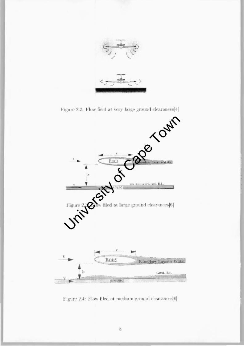
2.2 Flow field at very large ground clearances[4] 8
2.3 Flow field at large ground clearances[6] . . 8
2.4 Flow field at medium ground clearances[6] 8
2.5 Flow field at small ground clearances[6] . . 9
2.6 Flmv field at very small ground clearances[6] 9
2.7 Angle of attack relative to earth-fixed co-ordinate system 10
2.8 Aircraft axes[7] . . . . . . . . . . . 11
2.9 Calculation of aerodynamic centre. 12
3.1 Model with image support system in place[6] 21
3.2 Angular displacement of lift curve[6] 22
3.3 Angular rotation of polar curve[6]
3.4 Force diagram depicting D: 1Lp .[6]
3.5 Wing in normal configuration .
3.6 Wing in inverted configuration .
3.7 Wing inverted with full image support system
3.8 Body shape factor[6] .....
3.9 Tunnel-model shape factor[6] .
3.10 Drag components given by Maskelll61
IX
23
23
25
26
26
28
29
30
Univers
ity of
Cap
e Tow
n

4.1 Schematic of TEM balance . 33
4.2 Lab View Display Panel 35
5.1 TEM balance elevator 38
5.2 Elevator support frame 39
5.3 l\'Ioving-belt ground system 41
5.4 \Ving support system .... 43
0.0 DH AITU 10 - 40 - 2 - 10 - 2 - 60 - 21 - 5 \Villg 44
5.6 Final Configuration of Test Apparatus 46
5.7 Final Configuration of Test Apparatus 47
6.1 Typical ground experiment in the UCT McMillan Laboratory wind
tunnel .................. . 50
6.2 Change of model-weight moment with ex 51
6.3 DHMTU wing with full image support system 52
6.4 Normal and inverted CL 1).5. ex curves 52
6.5 Normal and inverted polar curves .. 53
6.6 DHMTU wing in normal configuration 54
6.7 DHMTU wing in inverted configuration. 55
6.8 Length of image tail strut ....... . 55
6.9 Additional length added to image tail strut. 56
6.10 Drag and moment from additional tail strut length 57
6.11 Moment transfer diagram 62
A.1 \Veight tare correction as function of ex 85
A.2 Calculation of tan exv.p' .. 86
A.3 Tare and interference data 87
A.4 Total blockage correction factor, Etotal 88
A.5 Variation of span efficiency factor, e, with ho 89
A.6 C L V.5. ex and ho ............... . 90
x
Univers
ity of
Cap
e Tow
n

A.7 CD VS. 0 and ho . 91
A.8 C M vs. 0 and ho 92
A.9 Polar diagrams . 93
A.10 L/ D vs. CL and ho 94
A.ll C M vs. C L for constant values of ho 95
A.12 Variation of aerodynamic centre in pitch with ground clearance 96
A.13 Cl\I vs. CL for constant values of a 97
A.14 oCL/oho and oCM/oho vs. ho . . . 98
A.15 Variation of aerodynamic centre in height with ground clearance 99
A.16 (CM vs. Cdh a=3 100
A.17 c.~!achl vs. ho . . 101
A.18 CM.ach2 vs. ho and C L . 102
B.1 Design drawings of DH MTU 10 - 40 - 2 - 10 - 2 - 60 - 21 - 5 ... 104
C.1 TEM balance elevator
C.2 Moving-belt ground system
C.3 v'ling support system .
C.4 Final tunnel assembly
Xl
106
107
108
109
Univers
ity of
Cap
e Tow
n

List of Tables
4.1 Tunnel parameters and ftow conditions . . . . . . . . . . . . . . . . . 32
4.2 Balance specifications and calibration constants . . . . . . . . . . . . 34
6.1 Test conditions . . . . . . . . . . . . . . . . . . . . . . . . . . . . .. 58
6.2 Solid blockage calculation parameters . . . . . . . . . . . . . . . . . . 59
6.3 Estimated values of Kl and Tl . . . . . . . . . . . . . . . . . . . . . . 60
Xll
Univers
ity of
Cap
e Tow
n

List of Symbols
AR
b
B
e
CDOmin
CDi
CD .min
CD.?
CD?e
CDS
CL
CLa
CLh
CL .max
e
h
H
ho
Kl
L
l
LID
LIDmax
M
aspect ratio
wmg span
test-section breadth
wing chord
test-section cross-sectional area
drag coefficient
profile drag coefficient
minimum profile drag coefficient
induced drag coefficient
minimum drag coefficient
parasite drag coefficient
equivalent parasite drag coefficient
drag coefficient due to separated flow
lift coefficient
oCLloa oCLloh maximum lift coefficient
moment coefficient
oCM loa oCMloh diameter of streamlined body
span efficiency factor
ground clearance
test-section height
relative ground clearance (= hie)
body shape factor
test-section length
length of streamlined body
lift I drag ratio
maxirnurn lift I drag ratio
pitching moment
Xlll
Univers
ity of
Cap
e Tow
n

J..1ach
AltT
J..1wt
q
Re
5
SSAJ
t
[T&I]low
[T&IL,p
U
V
V
VO[wing
w
Oup.total
(3
moment about the aerodynamic centre in pitch
moment about the aerodynamic centre in height
moment about the trunnion
moment correction due to model weight
dynamic pressure
Reynolds number
wing plan form area
static stability margin (= Xi! - Xo)
maximum wing thickness
tunnel-model shape factor
tare and interference on the side of the wing-lower surface
tare and interference on the side of the wing-upper surface
x - component of aircraft velocity vector
y - component of aircraft velocity vector
aircraft velocity vector
volume of wing
z - component of aircraft velocity vector
corn ponent axis on chord line
non-dimensional x- coordinate of ACP
non-dimensional x- coordinate of ACH
component axis perpendicular to chordline
angle of attack
equilibrium angle of attack
angle of attack due to upfiow
total angle correction
zero-lift angle of attack
angle of attack at stall
sideslip angle
solid blockage correction factor
wake blockage correction factor
total blockage correction factor
XIV
Univers
ity of
Cap
e Tow
n
Glossary
ACH ACP CFD Ekranoplan
LE
MAC
TE
VLM
\NrC
aerodynamic centre in height
aerodynamic centre in pitch
computational fluid dynamics
Russian term for ground-effect aircraft
leading edge
mean aerodynamic chord
trailing edge
vortex lattice methods
wing-in-ground-effect aircraft
xv
Univers
ity of
Cap
e Tow
n

Chapter 1
Introduction
1.1 Background to the Study
Ground effect is an aerodynamic phenomenon associated with a lifting surface op
erating in close proximity to another surface. Race cars typically use ground effect
to increase the downforce exerted on the car, which leads to improved traction. Air
craft typically use ground effect to increase the lift exerted on the wing, which leads
to a greater load carrying capacity. This report is concerned with the effect of the
ground on a wing for use on an aircraft.
Aircraft operating in close proximity to the ground experience significant changes
in the aerodynamic forces acting upon them. The result is usually characterised by
an increase in the lift and decrease in the drag on the wing; otherwise, an increase
in the lift / drag (L /D) ratio. It is recognised that most ground effect vehicles will
more likely operate as water-based craft, travelling over the ocean. As a result, some
vehicle design concepts are based on optimising an aircraft to safely fly close to the
ground/sea, while, others make use of ground effect to improve the performance
of fast boats. For this reason, these half-airplane/half-ship vehicles are collectively
referred to as "Wing-In-Ground-Effect" (WIG) vehicles. Because of the history and
strength of Russian technology in this field, many refer to WIG craft by its Russian
equivalent Ekranoplan (ekran - screen, plan - plane).
1.2 History
The phenomenon today known as ground effect was observed very early in the birth
of aviation. Pilots noted their aircraft tended to "float" in the air, when close to
the ground during landing. As early as 1921, the German Wieselsberger[lj was al-
1
Univers
ity of
Cap
e Tow
n

ready theoretically and experimentally analysing the effect of the ground on wings.
In 1935, a Finnish engineer, Kaario, designed one of the first craft engineered to
take advantage of ground proximity effects[2]. Throughout the Cold War era, the
Russian Rostislav Alekseev and the German Alexander Lippisch made significant
contributions to the field. However, it was not until 1967 that the West began to
take serious notice of the benefits of ground effect. This occurred when a US ana
lyst at the Defence Intelligence Agency identified a strange looking aircraft in some
satellite imagery taken over Soviet soil, near the Caspian Sea[3]. For a long time,
the very large plane was misunderstood as an incomplete aircraft due to its short,
stubby wings. Only later was it identified as a craft engineered to take advantage
of ground proximity effects, and became know as the Caspian Sea Monster. The
Caspian Sea Monster, launched in 1966 and known as the KM by its chief designer,
Rostislav Alekseev, was over 500 feet long and weighed 550 tons[4J. In 1995, a report
illustrated the interest in WIG technology with one of the largest WIG craft envis
aged to date[3]. An American company, Aerocon, conducted an investigation for the
US Department of Defence on the WIG craft's potential for strategic mobilityl. The
prospective WIG craft, called the AR-1, had a gross weight 5000 tons, a payload
capacity of 1500 tons and could cruise at over 400 knots (740 km/h). Compared
to a Boeing 747, the AR-1 was 12 times the weight, but had 30 times the payload
capacity, with a 44% improvement in operational efficiency2. Although the AR-1
was never built, this craft was conceived by the desire for a faster transportation
platform over water. However, for several reasons to be identified later, the KM
remains the largest WIG craft ever built to date.
1.3 Commercial Interest
WIG craft fill a large gap between low-costilow-speed shipping and high-cost/high
speed aircraft. A well designed WIG craft will have a relatively high L/D ratio of
15 to 30, and a cruise speed of 100 to 400 km/h[4]. This results in a very attractive
commercial and military transport platform, as identified by the KM and AR-1.
The Von Karman-Gabrielli diagram of figure 1.1 (a), illustrates the LID ratio of
various vehicles as a function of speed3. The technology line represents the limit
of the transport efficiency, the product of LID and speed, for all current forms of
transport. The shaded region clearly indicates the gap in transport efficiency, which
WIG craft typically fall into. Furthermore, the cruise power requirements per unit
weight, the P IvV ratio, are very low for WIG craft[4]. This is also illustrated in
figure 1.1 (b) in a comparison of WIG craft to other forms of transport.
1 The ability to project force on a global scale. 2Payload capacity per unit fuel consumed. 3For land-based vehicles the lift is simply the total weight of the vehicle.
2
Univers
ity of
Cap
e Tow
n

, L-________ ~ ____ ~ 100 1000 "" V lkrrVhJ ,- , .. ,~. , .. ~ V [km'hJ
How," "T 1. h"T{' a H' ,,., (,fa l 1 ino i 1m iOIl~ tIl 1 hI' llIl, kIt,! "",I i "v, ,,r t I", t '" Imol, ,~.y t lli-\1.
impact tl](' "')mnH''''i~ 1 "i~l,tl i t y of \\'Il~ ("mfll4l . S ... " ' ~ "fthc>;{' li""!:"'Oll' mdud(' ,
1. \fIG cr~ft are seusitiw 10 O('~aHl>l\raphi(" and dima\(' couditio!1s; such as ",aI'P
height and wind spl~'d. Smaller WIG cral'1 ar~ more sPusitiw to th.'s~ df,'c ts.
and ~n' t h,,, typieally Ie" efficient
2. All WIG n~[' ~re susceptible to pItch instability. which must be carefully
"x~rn iu{ ·d durlllg til(' d€l'.ign pro<·e".
~ Takillg off and lauding ill til<' s('a ""'n'~"'s til<' rksign nXluirc"l('nt.s in Wrms
of the airfranws s1ructural iut ('grit, aud add,tional "ngin.' I) '''' pc rt'quin>m" uts
w ",·,'IU"'l(' t he dra~ of the wa1er
Thpst' lhrt't' arl'as haw be('n t he ' mamstay for "H" h of t he n,,;~ard, "ond "ct ed in
prl'\io u~ ~'-l'ars. Th(' hrst two poinl~ lis t,>d abow, ha,e led to exten~i,e re~earth in
the arl'as of aIrcraft cOllfigurat,ion. pian[unn and wing proftle de~i)';n, The thi rd puint
IlHs i niti~led re:,e~rdl fo(us{·d at, millimi,in),; tak,'-ofl' power lequin'mmt, tll roU~h a
roouc1iou ill th (' tak, ~ofr dm !!, Thi~ is ath i,,\l''(\ t hrou~h th~' hull ,k"'i~n , the use of
h\drofoi ls ~nd PI",,'r a~si s",, 1 s\.a l ic ~ll LushioIl,I-t I, Wheu op€rati!1g ill uufa\'uurable
ciimah' condi tion'. t,he prubJ~lllb as"lXiat~d with t hp,,, t brel' points an' miuimi:;.t'ci
" l th wry larl':(' WIG nafl. Hmw\'er. tlH' cost of de\~l opi Il g larg,'r ("Taft. may nOT 1.><'
3
Univers
ity of
Cap
e Tow
n

politically, economically or sociologically feasible. As was the case with the AR-1,
with an estimated developmental cost of $60 billion dollars and a production cost
of $400 million dollars per vehicle[3].
1.4 Purpose of this Investigation
As identified above, there are limitations in WIG craft technology. The purpose of
this investigation is to develop the means for experimentally examining the forces
and moments on a wing in close proximity to the ground. Furthermore, to examine
the performance of a wing in the presence of the ground, and, examine the nature
of the stability of the wing in terms of the current literature. The investigation is
limited in that it only considers a single, arbitrarily chosen low aspect ratio wing.
The experiments are conducted in the low subsonic flow regime, with a test Reynolds
number of Re = 2.2 X 10⁵. The results are presented and the nature of the stability
determined in terms of the current literature. This report does not suggest any
methods for improving wing performance, nor present any solutions for the stability
problem usually associated with ground effect.
1.5 Description of the Main Problems Investigated
The main design problem was the design and construction of a moving-belt ground
plane for use in the UCT McMillan Laboratory wind tunnel. The original config
uration of the wind tunnel and associated instruments were adapted in order to
accommodate such a ground simulation device. This involved the design of a sup
port structure for positioning the existing three-component balance (L, D, M) in the
over-tunnel configuration. Furthermore, a device for changing the elevation of the
wing above the ground plane was designed, followed by the design of a new wing
support system.
The main research problem was the study of a wing in the presence of the ground.
The longitudinal performance of the wing in the presence of the ground was of pri
mary importance. This involved the capture of the lift, drag and pitching moment
versus angle of attack at varying ground clearance. A matrix of the lift, drag and
pitching moment data was then generated as functions of angle of attack and ground
clearance. The performance of the wing and the nature of the stability was then
determined as the wing entered ground effect.
4
Univers
ity of
Cap
e Tow
n

1.6 The Plan of development of the Thesis
The following chapter presents an overview of the basic aerodynamics in ground
effect, the general theory of longitudinal static stability in ground effect and vari
ous simulation techniques for ground vehicle experiments. Chapter 3 discusses the
treatment of flow interference in the test section. Chapter 4 identifies the existing
characteristics of the UCT McMillan Laboratory Wind Tunnel. Chapter 5 discusses
the design of the moving-belt ground plane and associated test apparatus. The full
test procedure is discussed in chapter 6, followed by the presentation and discus
sion of the results in chapter 7. The final two chapters present the conclusions and
recommendations derived from the results of the study.
5
Univers
ity of
Cap
e Tow
n

Chapter 2
Ground Effect, Longitudinal Stability
in Ground Effect and Ground
Simulation Techniques
2 .1 Introduction
Ground effect is an aerodynamic phenomenon associated with wings operating in
close proximity to the ground. The phenomenon is characterized by two separate
interactions[6]. The first concerns the interaction between the trailing vortex wake
system and the ground. The second concerns the nature of the airflow under the
body, which is strongly influenced by the interaction of the boundary layer forming
on the underside of the body, with the boundary layer on the ground, if it exists,
or with the ground itself. For positive angles of attack, below the stalled condition,
the influence of the ground, in general, produces an increase in the lift-to-drag ratio.
This arises as a result of the restriction in the development of the wing-tip vortices,
and, an increase in pressure between the wing and the ground. This usually only
becomes apparent at distances from the ground less than the length of the mean
aerodynamic chord (MAC). For this reason, the ground clearance is usually non
dimensionalised relative to the MAC of the primary lifting surface of the aircraft
in question. This description of the relative ground clearance will be denoted as
ho = hie, where h is the actual ground clearance and c represents the mean aero
dynamic chord of the wing (see figure 2.1).
Although there is generally a measurable change in the forces at values of ho = 1,
the effect tends to be most advantageous for the range of relative ground clearances
below 25% chord. Rozhdestvensky[2] categorizes very small relative ground clear
ances of less than 10% chord as extreme ground effect. He sites these small relative
6
Univers
ity of
Cap
e Tow
n

Figure 2.1: Measurement of ground clearance
ground clearances as the expected operational regime for future ground effect craft
due to significant iucreases in wing efficiency.
2.2 The Flow Field in Ground Effect
A wing will normally develop a boundary layer over its upper and lower surfaces.
Dependillg on the ground clearance, the presence of the wing will also induce a
bouudary layer on the surface of the ground as well as restrict the development
of the trailing vortices. Barlow et al.[6J identifies several basic classificatious that
describe the clearauce based on the level of interaction betweeu the trailing vortex
wake system and the grouud, and, the level of interaction between the boundary layer
ou the wing and the grouud. Together, with characterizations from van Opstal[4j
aud Ilozhdestvensky[2j, these classifications are broadly described as follows:
• Very Large Clearance (ho < b, ho > e). The presence of the grouud begins
to restrict the development of the trailing vortex wake system aud push them
outward (figure 2.2).
• Large Clearance (ho ~ e). The presence of the ground has a small influeuce on
the velocity distribution uuder the wing and the development of the bouudary
layer ou the wing. Induced flow is sufficielltly small so that no significant
bouudary layer develops ou the ground (figure 2.3).
• Medium Clearance (ho ~ O.5e). The presence of the ground has a cousiderable
iufluence on the wing and the wiug induces a significant boundary layer on
the ground. However, there still exits a well-defined region of potential flow
betweeu the two boundary layers (figure 2.4).
7
Univers
ity of
Cap
e Tow
n
-, ~ ,
, , , ~ .. ,~J, ",I " ,~"- III
-- ,
1 c 'iillW. -- .. -•
""" ,
, --,
,
Univers
ity of
Cap
e Tow
n

, , --
--Figure V i: FloI\' filed at H'fy small ),;T'JIlu ,l, 1('<I"lw Oj!; i6i
• Small (' k IlrUlW<' (hu" n,?;",], I h,' two t>O\lud;lJy !;wen< <I'" ~tp)ngly mterar-
1.'I'r. IlIl t n, t), 1i1,1 1<' n11 ',J uv, ''' Ibm t.he " ( rr~IIl",,r extent of th€ willg, Thl'r~
L, nO potrJ[ ' 1I1.1 H" w ,.-,p", ,, t illg t./l<' tw' , h" "lldM,I' la "er~ 'w{'[ nu" J, 0f lh~ "- '" ~.
lellgt h i li8me Vi)
• Yer." ~ml\lt C'learWlre ("" <: O, le) , Abo kJ I O"-~~;; n· t,r)n~ )';round dfe<:t a,
h" -. LJ Thi ~ iti the limit in r; "al*l wheI€ thr airflow ran ,r~I·. u. ' t " hrlrrw th€
wmg. Yi9<.:on'> force; domil late the mot lon 0[' the 110"- loetwer ll t hr "illg and
the ground. convective terms in t he l\m'iec-Stokc, '"'11l>\tim" I",,-,"'He negligible
3",\l.h<, How b~OIIles CS>.eul iall" c,,:eping flow (l1gm <' 2.61.
2.3 Longitudillal Stahility HI ground effect
III I !JJ:i, <I Fi[J[ll,h <,nginerr. Kaal io. desiv,ued one of th<' fir,t craft l' uglIlcrcl'd (0 take
advautagr of ground proximit.v r lT{'ct.Hi2i. II iH craft dcmollhtlalrd 'I jJ l td\ iu~t<tbi lit-y
which b 1101" recngll it.ed a" au iuhrrcur, d Lar<lct r riHt i,' of <Ill grollnd-eife( t n<lf!. The
, Iat ic lougitudmal stabi li ty of lifti ng "url'ac<.-,> ill l(Tound effect is evaluated by an
aua ly'" of the dl'ri \'ath 'es of t he lift coefficient, C i. and the UJOUlent. coeffic ir ll t. C.\!.
with respect 10 the pltch ll.TI"le. O. aTi d t he rel<lt i,·~ p;!"nu nd clearance. "o{eqnation
2,1 to ~A). T hIs alla ly"i, ai(l~ iJl u1J(lr"tamling t.lll' II>\tnrr of t,hl' rt"P"H'l' of <In
aircraft tn "arion, di'l llcball rrH The aforementioncd dPriYll.tivc, a rl' 'Hiftr ll ill (he
f"li m, ing way 1'01 rom"t'nirnce;
DC,lf
iJoj (2.1)
Univers
ity of
Cap
e Tow
n

XWlr1dlStabdlly
XBody
Figure 2.7: Angle of attack relative to earth-fixed co-ordinate system
(2.3)
(2.4)
At this point, it is important to recall the relationship between the pitch angle, e, and the angle of attack, 0:. The pitch angle, e, is the Euler angle measured between
a reference earth-fixed coordinate system and a body-fixed coordinate system on the
aircraft (see figure 2.7 and 2.8). The equilibrium angle of attack, 0: e , is measured
between the body-fixed axes and the stability axes!7]. Assuming zero sideslip angle,
(3, the stability axes are then aligned with the relative wind direction. Ignoring the
effects of wind/gusts, 0:e is then a function of the aircraft's forward and vertical
velocity components and is given by;
0:e = arctan (:) (2.5)
where the body-axes [x y z]components of the aircraft velocity vector are given by;
V= [UVWf (2.6)
The angle of attack, relative to the earth-fixed coordinate system is then given by
(see figure 2.7);
0:Earth = e + arctan (:) (2.7)
10
Univers
ity of
Cap
e Tow
n

BODY Z-AXIS
Figure 2.8: Aircraft Axes[7]
X-AXIS (WIND)
X-AXIS (BODY)
For an aircraft operating close to the ground, it is important to know whether CiEarth
is a result of the pitch angle, e, or of the vertical velocity component, W. For this
reason, e is the preferred variable for stability studies in ground effect, regarding
the derivatives of CL and CM in equations 2.1 through 2.4. However, for the wind
tunnel study in these experiments, the model is stationary. Therefore CiEarth = e, and, for simplicity, the variable Ci will be used for the remainder of this report.
Rozhdestvensky[2] identifies, through the works ofIrodov[8J, Kumar[9J, Staufenbiel[10]
and Zhukov[ 11 J, that the longitudinal static stability of a wing in ground effect de
pends on the location of the aerodynamic centres in height and pitch, and the
location of the centre of gravity. A discussion of these important parameters now
follows.
2.3.1 The Aerodynamic Centre in Pitch
The aerodynamic centre in pitch (ACP) is the point where CM remains constant
with changing angle of attack, Ci. Its definition is:
(2.8)
This expression gives the non-dimensional x-coordinates, relative to the moment
axis, of the ACP as a function of Ci. If body-fixed axes are used, the positive direction
of the x-axis is upstream and the values are given as a percentage of the wing chord.
11
Univers
ity of
Cap
e Tow
n

L
Aerodynamic Centre
a
••
Figure 2.9: Calculation of aerodynamic centre
Since CM and CL are functions of ho as well, the value of Xn VS. 0' must be calculated
with the data from each value of ho. The resolution of the ACP by equation 2.8, is
limited in that it only defines the movement of ACP along the chordline (assuming
the moment axis lies on the chordline). However, the ACP usually lies very close to
the chordline. Therefore, the vertical displacement is frequently not calculated. The
true location of the ACP can be calculated as follows (see figure2.9). If the distance
along the chord from the reference moment axis to the ACP is x, the distance
below the chordline is z and the mean wing chord is Co then the moment about the
aerodynamic centre in pitch, A1acn , is given by;
lVlac.n lv1Ref - xL cos 0' - zL sin a - xD sin 0' + zD cos 0'
lv1Ref - x(L cos 0' + Dsina) - z(Lsina - Dcosa) (2.9)
Where M Ref is the reference moment axis. In coefficient form;
x Z CM .ae .n = CM .Ref - - (CL cos 0' + CD sin 0') - - (CL sin 0' - CD cos 0')
C C (2.10)
Differentiating with respect to CL and applying the condition that the moment
remains constant with CL 1, the equation becomes;
= 0 = aCMRef
BCL
1 Since C L is approximately proportional to (} at small to medium angles of attack, can differentiate W.r.t. CL or (}.
12
Univers
ity of
Cap
e Tow
n
x [( [Ja ) ( [JC D [Ja ) 1 --;; 1 + CD [JCL
COS a + [JCL
- C L [JCL
sin a
-- CL-- - -- cos a + 1 + CD-- sina z [( [Ja [JC D) ( [Ja ) 1 c [JCL [JCL [JCL
(2.11)
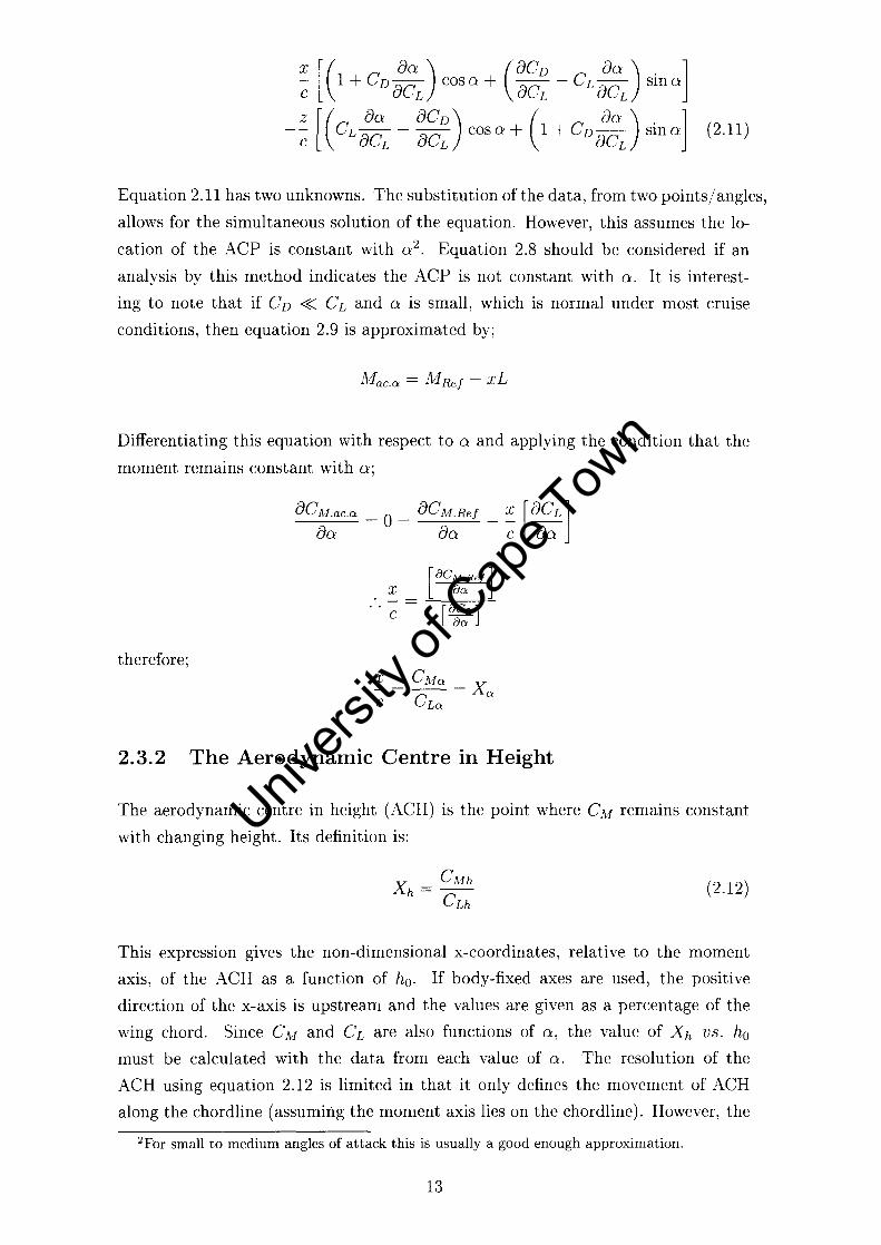
Equation 2.11 has two unknowns. The substitution of the data, from two points/angles,
allows for the simultaneous solution of the equation. However, this assumes the lo
cation of the ACP is constant with a 2. Equation 2.8 should be considered if an
analysis by this method indicates the ACP is not constant with a. It is interest
ing to note that if CD « CL and a is small, which is normal under most cruise
conditions, then equation 2.9 is approximated by;
Mae.n = M Ref - xL
Differentiating this equation with respect to a and applying the condition that the
moment remains constant with a;
therefore;
[JCM .ae.n = 0 = [JCM .Ref _ :. [[JCLl [Ja [Ja c [Ja
x
c
[8C~~Re! ]
[8faLJ
2.3.2 The Aerodynamic Centre in Height
The aerodynamic centre in height (ACH) is the point where CM remains constant
with changing height. Its definition is:
(2.12)
This expression gives the non-dimensional x-coordinates, relative to the moment
axis, of the ACH as a function of ho. If body-fixed axes are used, the positive
direction of the x-axis is upstream and the values are given as a percentage of the
wing chord. Since CM and CL are also functions of a, the value of X h vs. ho
must be calculated with the data from each value of a. The resolution of the
ACH using equation 2.12 is limited in that it only defines the movement of ACH
along the chordline (assuming the moment axis lies on the chordline). However, the
2For small to medium angles of attack this is usually a good enough approximation.
13
Univers
ity of
Cap
e Tow
n

ACH usually lies very close to the chordline. Therefore, the vertical displacement is
frequently not calculated. The true location of the ACH can be calculated as follows
(see figure 2.9). If the distance along the chord from the reference moment axis to
the ACH is X, the distance below the chordline is y and the mean wing chord is c,
then the moment about the aerodynamic centre in height, Mac.h , is given by;
M ac.h
In coefficient form;
M Ref - xLcoso - zLsino - xDsino + zDcoso
MRef - x(Lcoso + Dsino) - z(Lsino - Dcoso) (2.13)
(2.14)
Differentiating with respect to ho and applying the condition that CM remains con
stant with ho, equation 2.14 becomes;
OCM.ac.h oho
0= OCM .Ref
oho
-- 1 + CD-- coso + -- - CL-- sino X [( 00 ) (OC D 00 ) 1 c oCL oCL oCL
-- CL-- - -- coso + 1 + CD-- sino Z [( 00 oC D) ( 00 ) ] c oCL oCL oCL
(2.15)
Equation 2.15 has two unknowns, and substitution of the data, from two values
of ho, allows for the simultaneous solution of the equation. However, this assumes
the ACH is constant with ho, but this is frequently not the case. Thus, equation
2.12 is preferred for resolving the ACH. It is interesting to note that if CD « CL
and 0 is small, which is normal under most cruise conditions, then equation 2.13 is
approximated by;
M ac.h = M Ref - xL
Differentiating with respect to ho and applying the condition that CM remains con
stant with ho;
OCM .ac.h = 0 = OCM .Ref _ ~ [OCL] oho oho coho
x [aCMRe f ]
aha
c [~] aha
therefore;
14
Univers
ity of
Cap
e Tow
n

2.3.3 The Stability Criterion
A ground-effect craft must be stable in both height and pitch. A disturbance in
pitch angle or in height above the surface, must be compensated for by a restoring
moment or force. This tendency to restore equilibrium is known as positive stiffness.
Static pitch stability or positive pitch stiffness is associated with a negative slope of
the CM vs. Q: curve and is represented by;
(2.16)
For a trimmed aircraft, this provides a negative pitching moment for an increase in
angle of attack. Static height stability is also associated with a negative slope of the
CL vs. ho curves and this is represented by;
(2.17)
An increase in height would thus result in a decrease in lift. However, the above
condition is only valid when CM is held constant (held at zero for a trimmed aircraft).
The moment coefficient usually changes with height, and this change must be taken
into account. The condition for static height stability in longitudinal motion, given
by Staufenbiel and Kleineidam[10] and Zhukov[ll]' representing the combined pitch
and height stability criteria is;
By assuming height stability, CLh < 0, the expression can be simplified to;
Xh-X ____ a> 0 Xoo
(2.18)
(2.19)
Irodov[8] effectively came to the same expression, indicating that static height sta
bility is ensured if the aerodynamic centre in height is located upstream of the
aerodynamic centre in pitch. It is important to note that equations 2.18 and 2.19
were derived with the coordinate system located at the trailing edge of the wing,
and with the x-axis directed upstream. Therefore, the sign of X h and X oo , and hence
the inequalities, could be affected if the reference axis is located upstream of the
trailing edge. However, Irodov's criterion for static height stability holds regardless
of the reference point, specifically;
(2.20)
15
Univers
ity of
Cap
e Tow
n

The distance between the aerodynamic centres is referred to as the Static Stability
Margin, SSM = X h - Xo., and is required to be positive for static height stability.
The magnitude of the SSM also aids in predicting the nature of the response of the
wing to a disturbance.
2.4 Ground Effect in Wind Tunnels
I1ozhdestvensky!2J identifies two principal mathematical techniques for studying
ground effect, namely, numerical methods aud asymptotic approaches. Wieselsbergerl1 J
was one of the first to apply asymptotic methods to ground effect by employing
Prandtl's lifting line theory and the method of images. Ilozhdestvensky uses the
method of matched asymptotic expansions, first proposed by vVidnall and Barrowsl12J,
for the treatment of lifting surfaces in ground effect.
Numerical-based studies have made a significant contribution to the field of ground
effect aerodynamics. Huminic and Lutzl13j used CFD methods to study ground
simulation techniques. Chun and Park!14, 15] used potential based panel methods
to predict the influence of waves on a wing, while Pienaar! 16J used Vortex Lattice
Methods (VLM) for his treatment of the aerodynamic forces and moments.
Experimental methods, usually carried out in wind tunnels, form an integral part of
all aerodynamic studies. The treatment of the ground effect phenomenon in wind
tunnels is very important. The complex flow field generated when a wing operates
close to the ground, increases the need for reliable experimental data. Barlow et
aL[6] identify several systems used for simulating the ground in wind tUIlIlels, and
are discussed below.
2.4.1 Fixed-Floor Wind Tunnel
A basic fixed-floor, closed test-section wind tunnel will have a developed boundary
layer on the floor. The ratio of the relative wing ground clearance to the relative
floor boundary layer thickness is critical. When the incoming floor boundary layer
is thick, relative to the wing ground clearance, the flow about the wing can be
significantly modified. Thus, measurements made with fixed-floor tunnels must be
interpreted very carefully. Currently this is not a recoIIlmended practice.
16
Univers
ity of
Cap
e Tow
n
2.4.2 Symmetry /Method of Images
The method is based ou modelliug the grouud as a streamliue (Euler wall). Two
identical models are constructed. One is inverted relative to the other to form a
plane of geometric symmetry. The plane then represents the ground. For model
geometries and Reynolds numbers that result in a steady flow over larger ground
clearances, the method of images is suitable for simulating a moving ground plane.
However, symmetric geometry does not always produce a symmetric flow patteru,
and the mean airflow is not always steady. Furthermore, this method does not
simulate an induced ground boundary layer as expected at smaller clearances. Model
costs are also doubled for each experiment. Barlow et aLl6j suggest the ratio of the
model frontal area to test-section cross-sectional area should not exceed 7.5% unless
errors of several percent are tolerable. Since two models are required, this guideline
restricts the size of the model. Serebrisky and Biachuevl17j examine a Clark Y-H
airfoil with AR 5 using this method. Fink and Lastingerl18j use this method to
examine a rectangular wing of several aspect ratios.
2.4.3 Elevated Ground Plane
The elevated ground plane is a thin plate mounted parallel to the tunuel floor.
It is usually positioned above the tunnel floor boundary layer. A new, thinner
boundary layer theu begins to form on the elevated plate. This technique is simple
to implement, but the problem of the boundary layer still exits. Flow perturbations
may arise due to the presence of the plate and hence cause changes in the flow field.
The arrangement also causes a split flow on either side of the plate that is iufluenced
by the model, which in tum makes accurate determination of the effective airspeed
difficult. Support of the model can also be troublesome. This method was widely
used until the 1970's but is rarely used today. Furlong and Bollechl19j analyse a
swept back wing using this method.
2.4.4 Raised Floor: Suction at Leading Edge
This method uses a blower/fan, mounted at the leading edge of a raised floor in the
test-sectioH, to remove the low energy air from the tunHel floor boundary layer. The
air is re-injected back into the airstream at the downstream end of the test-section.
The result is similar to that of the elevated ground plane; however, there are two
main advantages. The floor and ceiling pressures can be made equal at the entrance
to the test-section through control of the blower setting. This aids in improving the
flow uniforInity (Le. reducing flow angularity). The raised floor need Hot be raised
as much as the elevated ground plane, therefore having little impact on the effective
17
Univers
ity of
Cap
e Tow
n

area available in the test-section.
2.4.5 Suction through a Perforated Floor
There are two variations in the way the perforated floor is used. The first uses suc
tion applied under a perforated floor segment upstream of the model. Depending
on the amount of suction applied, the boundary layer thickness is reduced over the
perforated segment. However, the boundary layer begins to grow again after the
perforated segment. The result is similar to that of the raised floor with suction
at the leading edge; however, there is a delicate balance between induced flow an
gularity and boundary layer thickness. Usually small amounts of suction are used
in conjunction with other methods. The second variation utilises distributed per
forations throughout the test-section. This system can remove the boundary layer
altogether, but cannot simulate the moving ground plane with precision. Again, a
compromise between induced flow angularity and boundary layer thickness must be
made.
2.4.6 Tangential Blowing
With tangential blowing, air is injected parallel to the airstream, through a thin slot
along the tunnel floor upstream of the model. The floor jet energises the boundary
layer by replacing the lost momentum due to viscous effects. The boundary layer
grows normally downstream of the jet. Tangential blowing has been found to pro
duce drag results close to that of a moving ground, but other measurements can
differ considerably.
2.4.7 Moving Ground Plane
This method uses a moving belt as the effective floor of the tunnel. In general, it
is desired that the belt speed matches the air speed in the test-section. Operating
conditions are simulated best; however, there are several disadvantages. Currently,
there are few belt systems capable of approaching 100 m/ s due to the complexity
and cost of such systems. The other disadvantage is that the model generally needs
to be supported from the top or sides of the test section. Tests involving a low
pressure difference between the model and the belt have a tendency to lift the belt
off the floor. This must be counteracted by suction on the underside of the belt.
Kim and Geropp[20] used a moving ground plane, in conjunction with a leading edge
perforated floor, to examine the flow over two-dimensional bluff bodies. Turner[21]
analysed the flow over two high lift models using a moving-belt ground plane in
18
Univers
ity of
Cap
e Tow
n

conjunction with a leading edge suction device, and, assisted by a perforated floor.
Furthermore, he determined a physical limit, based on the lift to ground clearance
ratio, for testing high lift models with an elevated ground plane. He found an
elevated ground plane produced satisfactory results for C L < lOho. For CL > lOho,
a moving-belt ground plane was recommended.
2.5 Concluding Remarks
The moving ground plane best simulates the flow conditions in ground effect. It is
expected that the tests will be conducted at ho < 0.1 and CL > 1. Thus, based on
the recommendations of Turner[21]' a moving ground plane should be used. As will
be identified in the next chapter, the wind tunnel available for this experiment is
relatively small and has a maximum airspeed of approximately 30 mj s. Thus, the
demands on the ground plane are not as severe as larger, faster wind tunnels.
19
Univers
ity of
Cap
e Tow
n

Chapter 3
Treatment of Flow Interference in
the Test-section
3 .1 Introduction
Flow conditions in a wind tunnel are never exactly the same as those that would be
experienced by the same model in an open unrestricted environment. Two important
factors that influence the flow conditions are;
1. the effects of the wing support system.
2. the effects of the test-section boundaries.
The tunnel airstream is usually not perfectly parallel and uniform throughout the
test-section. There is usually some induced flow angularities due to the presence
of the wing support system, windshields and the model itself, however, flow angu
larities may also exist in an empty test-section. The flow angularities can occur
in any streamwise direction; that occurring in the vertical direction is collectively
referred to as upflow, and that occurring in the horizontal direction is referred to as
cross-flow. However, upflow is considered more important as it affects the accuracy
of the drag. The existing "empty test-section" upflow and that induced by the pres
ence of the model, is evaluated and corrected for in section 3.2. The interference
caused by the interaction of the airflow with the wing support system, the wind
shields, and the model, is evaluated in section 3.3. It is important to note that in
both cases the model configuration, the model attitude and dynamic pressure also
influence the airflow; hence, each unique test requires a unique correction.
The presence of test-section boundaries, whether solid plus a boundary layer, or
still air plus shear layers, produce several effects that would not be experienced in
20
Univers
ity of
Cap
e Tow
n
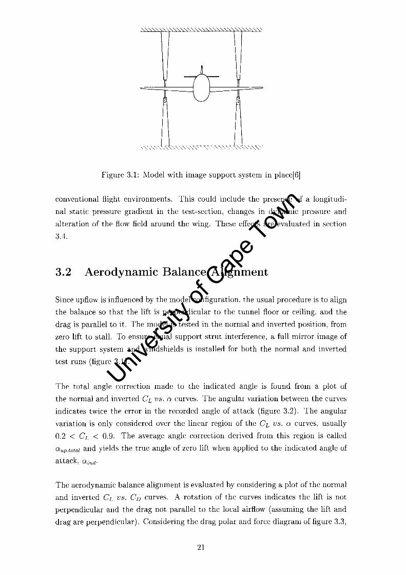
Figure 3.1: Model with image support system in place[6j
conventional flight environments. This could include the presence of a longitudi
nal static pressure gradient in the test-section, changes in dynamic pressure and
alteration of the flow field around the wing. These effects are evaluated in section
3.4.
3.2 Aerodynamic Balance Alignment
Since upflow is influenced by the model configuration, the usual procedure is to align
the balance so that the lift is perpendicular to the tunnel floor or ceiling, and the
drag is parallel to it. The model is tested in the normal and inverted position, from
zero lift to stall. To ensure equal support strut interference, a full mirror image of
the support system and windshields is installed for both the normal and inverted
test runs (figure 3.1).
The total angle correction made to the indicated angle is found from a plot of
the normal and inverted CL vs. Q curves. The angular variation between the curves
indicates twice the error in the recorded angle of attack (figure 3.2). The angular
variation is only considered over the linear region of the CL vs. Q curves, usually
0.2 < CL < 0.9. The average angle correction derived from this region is called
Qup.totai and yields the true angle of zero lift when applied to the indicated angle of
attack, Qind.
The aerodynamic balance alignment is evaluated by considering a plot of the normal
and inverted CL VS. CD curves. A rotation of the curves indicates the lift is not
perpendicular and the drag not parallel to the local airflow (assuming the lift and
drag are perpendicular). Considering the drag polar and force diagram of figure 3.3,
21
Univers
ity of
Cap
e Tow
n

c5 "i
1.4 ..... .
1.2
1.0
.~ 0.8 :E Q)
8 3 0.6
0.4
0.2
0.0 '------'---"-5 o
Model normal ---1"-/
~-- True lift curve
Model inverted
5 10 a,degrees
15
Figure 3.2: Angular displacement of lift curve[6]
part of the lift is appearmg as drag; with the lift decreasing the drag when it is
positive and increasing it when it is negative. The true drag value is related to the
indicated value (wing normal) by the following expression (see figure 3.4):
CD.true C D .ind + CL.true sin Q up
CD .ind + CL .ind tan Q up
Therefore, Q up is found as follows;
tan Q up CD.true - C D .ind
CL .ind
0.5 (CD .inv - CD .ind )
CL .ind
0.5~CD
CL .ind
The correction to the indicated drag is given by:
D true = D ind + ~D
where;
~D = Lind tan Q up
22
(3.1 )
(3.2)
(3.3)
(3.4)
Univers
ity of
Cap
e Tow
n

1.2 -
1.0
I c.J" .... 0.8 f----+----+--+:L>If-----f----t--------l c '" 'u :E '" o ~ 0.6 :::i
OA
0: L------L..-'----L.L~; ._._-----l.--._-.. - ---.J
o 0.01 0.02 0.03 0.04 0.05 0.06 Drag coefficient, C [)
Figure 3.3: Angular rotation of polar curve[6]
-------
~ Relative wind
Tunnel 8 balance ~
Figure 3.4: Force diagram depicting O:up.[6]
23
Univers
ity of
Cap
e Tow
n

The true lift value is given by the expression:
L true = COSDup
(3.5)
However, Dup is usually small enough such that L true = Lind and no correction is
applied. If the indicated angle of attack on the balance is correctly aligned with the
incidence arm, the wing, and the tunnel floor, then Dup.total = Dup. This implies the
angular correction is due to local flow angularities only. If they are not equal, an
error exists between the alignment of the indicated angle, the pitching mechanism
and the tunnel floor. The source of such errors should be assessed to determine its
impact on the data. Nevertheless, the angular correction Dup.total includes D up , and
is the only correction applied to the indicated angle of attack.
D = Dind + Dup.total (3.6)
3.3 Tare and Interference
The airflow around any model supported in a wind tunnel will be exposed to some
level of interference due to the presence of the wing support system and any other
devices in the airstream (such as strut windshields). The interference or modification
to the airflow will affect the forces and moments on the model and must be properly
accounted for. However, since different models and dynamic pressures also produce
different flows, which interact with the wing support system, the level of interference
on the forces and moments will be unique for different test conditions and model
configurations. When the airstream is influenced by the wing support system, the
effect is called interference, while the direct drag on the support structure is referred
to as tare. The two effects are collectively referred to as, tare and interference (T&I).
For a particular model and dynamic pressure, the T &1 effects can be found for the
combined influence of the main and tail support struts (including windshields). This
method required three tests with the wing in three different configurations, namely;
1. the wing supported in the normal configuration.
2. the wing supported in an inverted configuration.
3. the wing supported in an inverted configuration with a mirror image of the
full support system in place.
The support system and windshields of a normal test run will influence the lift, drag
and pitching moment as follows (figure 3.5):
24
Univers
ity of
Cap
e Tow
n

Figure 3.5: Wing in normal configuration
Lind Lnorm + [T &I]up.L
Dnorm + [T&I]up.D (3.7)
where [T&Ilup represents the tare and interference for each component (L, D, M),
due to the support and windshield system on the side of the upper surface of the
wing. The inverted model will yield the following (figure 3.6):
Lind Linv + [T &I]low,L
Dinv + [T &I]low,D (3.8)
Mind Minv + [T&I]low,M
where [T&I]low represents the tare and interference due to the support and wind
shield system on the side of the lower surface of the wing. The inverted model with
the image support system and windshields gives the combination of the two effects,
namely (figure 3.7):
Lind Linv + [T&I]low,L + [T&I]up,L
Dinv + [T&I]low,D + [T&I]up,D (3.9)
Mind Minv + [T&I]low,M + [T&I]up,M
25
Univers
ity of
Cap
e Tow
n
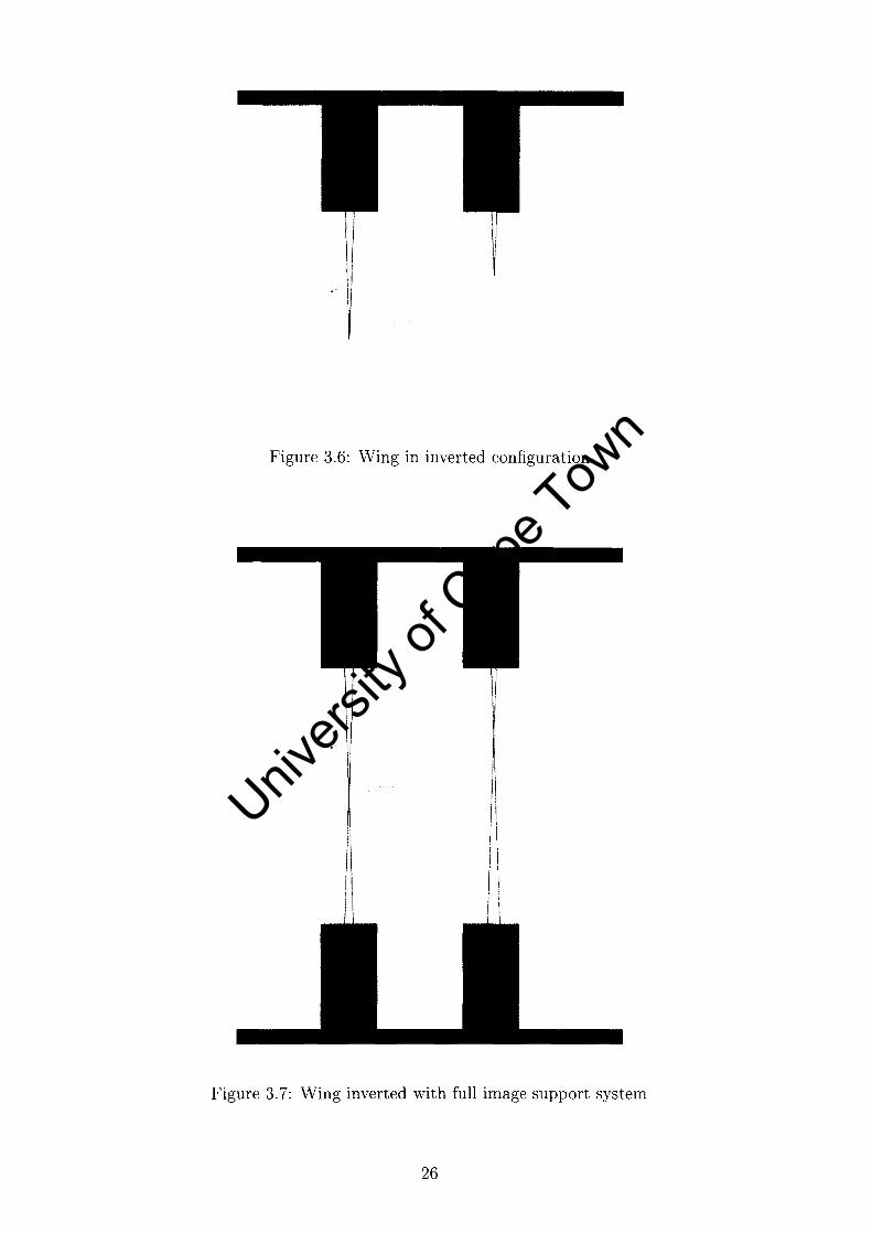
Figure 3.6: Wing in inverted configuration
.1
Figure 3.7: Wing inverted with full image support system
26
Univers
ity of
Cap
e Tow
n

The difference between equations 3.9 and 3.8 yields [T&I]up' for each component,
experienced by the wing supported in the normal configuration. The values of
[T &I]up' which change with angle of attack, are simply subtracted from the wing
normal data represented by equation 3.7. It is required that all the above corrections
are applied before boundary corrections are evaluated.
3.4 Boundary Corrections
The existence of the test-section boundaries produces several effects not experienced
in conventional aircraft environments. Since these effects are a consequence of the
finite size of a wind tunnel test-section, many of these effects are minimised by
reducing the model size to tunnel size ratio. The relevant boundary corrections are
evaluated as listed below[6];
1. horizontal buoyancy
2. solid blockage
3. wake blockage
4. normal downwash correction
5. tail downwash correction
6. streamline curvature
7. spanwise downwash distortion
The experiments described in this thesis are conducted in an open test-section wind
tunnel, with a moving belt installed to simulate the effect of the ground. For ground
effect studies, the force and moment data is usually only corrected for solid and wake
blockage and, if required, horizontal buoyancy[6]. The remainder of the boundary
corrections are usually not applied since the model is close to the tunnel floor. Thus,
the remaining boundary effects due to the side walls and ceiling are considered
negligible in comparison to the ground effects. Many open test-section tunnels
have approximately zero horizontal buoyancy. As will be identified later, the static
pressure gradient, and hence the horizontal buoyancy, are approximately zero for the
tunnel used in these experiments. Horizontal buoyancy is also usually considered
insignificant for wing only experiments. For these reasons, the horizontal buoyancy
correction term is also neglected.
27
Univers
ity of
Cap
e Tow
n

1.10 .----..,...----r------r----;----,
1.06 f-----~--___+---t_-r-w"'7$'q_--___t
1.02 f------'--
~ "0 fi 0.98 I----==F~£..._,~I__--_+--___i---_i
~
0.94 f-------=--+----+--------:~~----I
0.90 I------",.~
0.86 '-__ ...I.-__ --l. ___ '"--__ -'-__ -'
0.04 0.08 0.12 0.16 0.20 0.24
Thickness ratio f or 1
Figure 3.8: Body Shape Factorl6]
3.4.1 Solid Blockage
Solid blockage refers to the ratio of the model frontal area to test-section area. The
ratio is effectively zero in free-air; however, in a wind tunnel it is advisable to limit
the ratio to less than 7.5%16]. Relative to the free-air condition, solid blockage causes
an increase in the surface shear stresses in a closed test-section, and a reduction in
surface shear stresses in an open test-section. The effect is more pronounced in closed
test-section tunnels and is compensated for by considering the effect to produce a
change in the dynamic pressure, q, at the wing. Thus, the correction for this effect
is made to the dynamic pressure before the forces and moments are reduced to
coefficient form. For a wing in a closed test-section:
Kl Tl Vol wing Esb.closed = C1.5 (3.10)
Where;
• Kl - body shape factor (figure 3.8)
• Tl = tunnel-model shape factor (figure 3.9)
• VOlwing~ volume of the wing
28
Univers
ity of
Cap
e Tow
n

1.1 .----"""'T'------,---.....,---~--___,
1.0 I-----+-----f'""'oooo;;;:::-----+----t-----;
0.8 b==~l~.O~O~~~:1~~::~--1_----J
0.7 L--__ --'-__ ---' ____________ ____
o 0.2 0.4 0.6 0.8 1.0 Model geometric span _ b
Tunnel breadth - B
Figure 3.9: Tunnel-Model Shape Factor[6j
• C ~ frontal area of test-section
• I=- max wing thickness to chord ratio c
• 1 = streamlined body diameter to length ratio
For an open test-section:
Esb.open = ~O.25Esb.closed (3.11)
If the airfoil volume is not known, the following estimate is considered acceptablel6j;
Volwing = O.7(t)(MAC)(b) (3.12)
Where;
• t ~ maximum wing thickness
• MAC = mean aerodynamic chord
• b ~ wing span
29
Univers
ity of
Cap
e Tow
n
CD
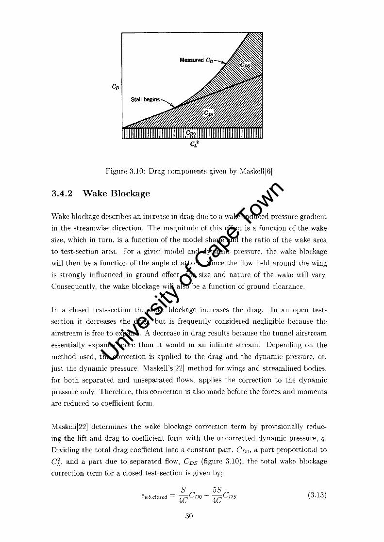
Figure 3.10: Drag components given by Maskelll6]
3.4.2 Wake Blockage
Wake blockage describes an increase in drag due to a wake-induced pressure gradient
in the streamwise direction. The magnitude of this effect is a function of the wake
size, which in turn, is a function of the model shape and the ratio of the wake area
to test-section area. For a given model and dynamic pressure, the wake blockage
will then be a function of the angle of attack. Since the flow field around the wing
is strongly influenced in ground effect, the size and nature of the wake will vary.
Consequently, the wake blockage will also be a function of ground clearance.
In a closed test-section the wake blockage increases the drag. In an open test
section it decreases the drag, but is frequently considered negligible because the
airstream is free to expand. A decrease in drag results because the tunnel airstream
essentially expands more than it would in an infinite stream. Depending on the
method used, the correction is applied to the drag and the dynamic pressure, or,
just the dynamic pressure. Maskell'sI22] method for wings and streamlined bodies,
for both separated and unseparated flows, applies the correction to the dynamic
pressure only. Therefore, this correction is also made before the forces and moments
are reduced to coefficient form.
Maskell[22] determines the wake blockage correction term by provisionally reduc
ing the lift and drag to coefficient form with the uncorrected dynamic pressure, q.
Dividing the total drag coefficient into a constant part, CDO , a part proportional to
Ci, and a part due to separated flow, CDS (figure 3.10), the total wake blockage
correction term for a closed test-section is given by;
(3.13)
30
Univers
ity of
Cap
e Tow
n

\Vhere;
• S -=- wing planform area
CDi is the induced drag which arises from the wing-tip vortices formed by a finite,
lift producing wing. CDi is proportional to C'i. CDO is the profile drag and defined
as that component of the total drag due to viscous effects, consisting of skin friction
and form drag. For angles of attack below the stall angle, the term CDS is usually
zero. For an open test-section, the correction is negative and smaller, and, the
following relation is used.
Ewb.apen = -O.25Ew b.clased (3.14)
3.4.3 Application of Solid and Wake Blockage Correction Terms
The final blockage correction is given by:
Etatal = Esb + Ewb (3.15)
The corrected tunnel velocity is given by:
Vc = Vu (l + Etatal) (3.16)
The corrected dynamic pressure is given by:
(3.17)
31
Univers
ity of
Cap
e Tow
n

Chapter 4
UCT McMillan Laboratory Wind
Tunnel
4.1 Tunnel Parameters and Flow Conditions
The UCT McMillan Laboratory wind tunnel is a closed return wind tunnel. The
test-section has an octagonal profile jet and can operate in an open or closed test
section configuration. Some of the key features of the tunnel are listed in table 4.1.
The values indicated for the static pressure gradient and the turbulence intensity
are for open test-section operation.
For the experiments described in this thesis, the tunnel operated in an open test
section configuration. This allowed easy access for model changes and positioning
of the instrumentation.
Table 4.1: Tunnel Parameters and Flow Conditions
Height, H 0.580 m Breadth, B 0.876 m Length, L 1.600 m
Fillet Height 0.146 m Section Area, C 0.453 m 2
Tunnel Aspect Ratio, B IH 1.51 -
Maximum Test Velocity ~ 30 mls Static Pressure Gradient, dp I dl ~O Palm
Turbulence Intensity 0.4 %
32
Univers
ity of
Cap
e Tow
n

FO;G6S ",m.--
~.b'n Support Struts ------- ~-----T"" Strut •
Fi~uw·U ~kh"'llIalie IJf TE:\! llalall'.T
4 .2 Tllp Force Balance S peci fi cat,ioHs a nd C ali bra
t ion
Th,' fOll<' hi\I~Jln' '" ~ 1!J~{j '1'1-:\1 F1Wl" r~ ""r: ',.odd ii'll; , :1·"o"'l'oO""t. paran",1
",ot io" !} pr h" hH L'P (fi&HIP 4. I ) Ir "~." "IX'I ~((, I" ~H "od"1 "1 oWr ·rllooel ( ·onli~n·
rat ion. Tit", model '''(,(,01 t ~y~t~lll i~ lll' "J11f(~1 "0 H f01 C% [nnw, ,\ hlt'h I, ,n~p"ndh ]
D,' a l'o UIJ I",d ]""am ~s~embly I I"" lift ,,,, eI dr~g l"vre..:, act throll~h th~ [IJrCK f,aH 'f.
wludl IranHfel'~ th", l oael~ to two ~\1Hil1 gHUg'" tra,,~rlueerg. '[he I'jkhin~ nwnu,,,j
ads, ,ia a tail strut. ()n an in("id l'nle ~nll rnOUllt",d ()Il thl, [IJre~ [ram"" lhe iun·
deuce anll trallsfer~ the lo~d tD anoth",r tram;du{'{'r and is also used to set the au~le
of HrtHek. I hI' halam:(' 1ll0lUI'I.lt celltre (the point about whieh the mom('ot is mCa·
~lJ1l~l) H('r~ Hho"t rhe pi\'()t j)<, int ()f the lUall.llUodd support ~tr"ts. It is illlj)<>r!.a"t
t hat th~ main ~truts &Ie I'NI'('mheu1 H1 to I.hl' f()n'ps frHllle ami I.hHt till' tail strut
remains paraHl'l to th", m~il1 stmt.~ hlIthNlllor('. thl' ;"(";01",",,,, HrHl TtlU,t wmain
paraU",llu the line bel\H'('11 r.l"" pl V"I.~ ()f t. h(' lllHio H"d tlt(' tHil ~t]'lJts. titus form;Hg
II parallelolirarll.
I h", halanc", ("alib1 Ht i"" was dlCCk('d usil.lli the supplic.-J ("alibratwo NIUI ptll('n!.. '.I his
cou,isted of:
a calibration frame, which was attached to th", mudd suppurts 10 simulate the
model under test.
2. a pll iley [or r/", "-i'plicatiou of dra~ loads.
:L a r.et of accur«te "~i!11lts and tW() ",'H lr pao" 1.0 Sllpport tlw individllHI weights
:\ lift fore" "as al'p li,'d to the ba.lHJ](·{· by the additiun u[ .... eights to the cHlibra!ioll
fr~ltLe. Omg WHS applied via" iwri.wl.ltal "ire attached 10 the rear of the calibration
Univers
ity of
Cap
e Tow
n

Table 4.2: Balance Specifications and Calibration Constants
Component I Load Range I Accuracy I Calibration Constant I Lift 0- 90 N 0.222 N 111.489 N IV
Drag 0- 36 N 0.0890 N 39.555 NIV Pitching }.foment 0-1.70 N.m 0.0170 N.m 2.2249 N.mIV
I Incidence Range I _100 to + 400 I
frame and passlllg over the calibration pulley where the weights were hung. A
pitching moment was applied by shifting the positions of the scale pans 50 mm off
the moment axis. Weights were applied and the calibration checked. The load range,
transducer accuracy and recalculated calibration constants are given in table 4.2.
The lift / drag and lift I moment interaction was checked. Interaction in both cases was
less than 0.1 % and well within the transducer accuracy. Therefore, it was considered
negligible. Oil dashpots were provided to dampen turbulence-induced oscillations
in the mechanical linkages. Due to the high turbulence levels experienced at high
angles of attack during pre-tests, the oil was replaced with 80W90 weight oil to
increase the damping.
4.3 Data Acquisition
The original display ofthe body forces was made using a digital volt-meter. However,
the pre-tests indicated insufficient damping of the mechanical linkages due to highly
separated flows at high angles of attack. This resulted in rapidly changing data
values on the digital display, making accurate recording of the data difficult. It
was decided to capture the signals over a period of time and calculate the statistical
mean. The signals from the lift, drag and pitching moment transducers were sampled
at 100 Hz with a PCI-730 high performance data acquisition board. A virtual
instrument panel was constructed in Lab View to manage all data acquisition. The
forces and moments were displayed in real-time to help identify any peculiarities
during a test. Each signal was sampled for 30 seconds and processed to find the
statistical mean (figure 4.2). The appropriate scale factors were then applied. The
repeatability of the data was checked and found to be within the specified accuracy
of the balance. The data was then saved to an Excel spreadsheet for post processing.
34
Univers
ity of
Cap
e Tow
n

Univers
ity of
Cap
e Tow
n

Chapter 5
Experimental Apparatus Design
Procedure
The principle design task was to develop a moving-belt ground plane for use in the
UCT Mc:YIillan Laboratory wind tunnel. Furthermore, this involved the design of
several additional features to allow positioning of the ground simulation system and
the required instrumentation. A discussion of the design process of each element of
the final design now follows.
The TEM 3-component balance was previously operated in the under-tunnel con
figuration. Therefore, the balance would have to be converted to the over-tunnel
configuration and repositioned above the test-section for all subsequent tests. The
next design decision depended on the method used for adjusting the ground clear
ance. For cost and complexity reasons, it was decided not to utilise any system using
suction or blowing devices at this stage. This ruled out the possibility for changing
the ground clearance through the vertical displacement of the moving-belt system.
This method, like the 'raised floor: suction at leading edge' method, requires a fan
or blower to remove the flow from the leading edge of the exposed belt and the
re-injection of it at a downstream location. There was also insufficient room below
the test-section to accommodate the moving-belt system and an elevation system
by any simple means. An alternative method, such as that used by Turner[21]' in
volved the use of a telescoping model support strut. This was a favoured method.
However, the TEM balance consists of two leading edge struts and a tail support
strut. Synchronisation of all three struts was thought to be too complicated, and
led to the decision to fix the strut lengths and elevate the balance as a complete
unit. Based on this design methodology, each component of the test apparatus is
discussed below and the final configuration is shown in figure 5.6 and 5.7.
36
Univers
ity of
Cap
e Tow
n

5.1 TEM Balance Elevator
5.1.1 Design Criteria and Concept
Listed below are several design criteria that were considered important.
• The balance-elevator system must maintain alignment under aerodynamic
loading and changes in elevation.
• The change in elevation should exceed the half height of the tunnel. This will
allow testing at the centreline and at the ground.
• The change in elevation should ideally occur in the vertical direction only,
unlike a scissor jack which moves horizontally as it moves vertically.
Several designs were considered utilising various elevation-changing methods. How
ever, the primary concern was whether or not the elevation system could maintain
adequate alignment under the load of the aerodynamic forces and during an elevation
change.
5.1.2 Final Assembly
The final design consisted of two frames (figure 5.1). An outer framework supported
the four solid bar legs, while an inner framework was guided by the four legs. The
design incorporated a 300 mm elevation change. This was sufficient to move a wing
from the tunnel centreline to the tunnel floor. It was concluded that a design
incorporating four 30 mm diameter, bright mild steel solid bar legs, with phosphor
bronze bearing shells, would give adequate support and alignment. The advantage
of this system was that the balance would only move in the vertical direction. The
design was also very simple and a single overhead jacking system could be used.
The main disadvantage with the use of bearing shells was that perfect alignment
of the four solid bar legs and bearings was required to prevent them from binding
or pinching. A greater tolerance in the fit of the bearing shells could be used,
however, this would lead to greater misalignment under aerodynamic loads. The
design required that the entire frame be bolted together since heat induced in a
welded frame would have caused the bearing shells to distort. The assembly drawing
is included in Appendix C.
37
Univers
ity of
Cap
e Tow
n

~ ., .j. ~
• •
I' ;~ur" 5.1' I f:t.r H"hlu, ~ E!<cy;,.wr
C; k vat or SllP I10J' t F";U1 W
OUe\' th~ d .. ~i~1I lof t l: .. 1.> ... 1 ... ,,]0' .. 1<,I'a tor w ..... 1im.lised. II sllppmtJ :a~ flam,'"",k w;l..;
1'I,~'<i,'<i to ~iliofl t t. ... balann-"''',awr 5)'5;,·,;. ;;I'propri:l.ld~<. g.-.,·,-. n.l ,I''''SII Hift-I'i'l
Ihm W"ft' (""D,.,j~eretl ;"'l lOrtaol Ill" li.s."rl be:O\>
• fll., frll''''''''/Hk "~,,, Id h ~ \'(' \0 ~Hv" 11.1<' halan(t' f,) b<. ~h ift "' l f"r",'''! ;,. 11<1
h;(~k"H["(L Th j~ "ill a.n o", for dlm'n'ut ",,,I. \')('>It,, ,,, " in t be ,tR'Hm·"i .. · din'V
lioll.
• Th~ framework mu~t p o, iti'lIl 110 .. 1>;,.1 (11 [("'< loll t~id~ of t h .. shE-lit lfll", of the
!('st_""nio" jd . T h" .... ill pre'~nt possi llll' t llrl>u le r.fe-in.-!uH~ 1 ,,,,"llJ>tIL"U lrl
tl,,' .;"pl ~millg frdl"""·,,. l tha l II/J\\' IIp.'iI': No la llo' ali~m",·nt · ,r ,Ialll 'lu;\h"
• rhO' frallle"", " Ill .!-! not he (X(" ... ' 1\'\ h ' rar II.""Y fwm thl:' w'!~-,., rlOn hm.her
1l\\Il~ " ill rt'tluiw ""'gN " ,,:,It M' l'l'vrt 'U,,[~ ,,-hlt:h "'''Y Iwud "wi", II<'T' HII'
nlllllie lo.adi .:g_
• I II,' fra !l"""'or;-; mu~t all,,\\ c ... mpl t'l.' t<l,(:C!oO to the ",';nd tUJlI, el t~,.,t-M'('liou for
p"~It." ,,, iJlg uf III" mu.-iug-belt ,"r~tell ' all.! ~a",~ mudel cunti!iillU\[ivn d"'Il:::e~,
Univers
ity of
Cap
e Tow
n

". " " ... _.-
• • •
t' i nil I A:.;:.;1;-' t1l b 1 Y
1'1,,' hTl~1 (10."; '1\11 ~os~ltl l \ l r IS ,h"" 1\ ' 11 tijl1J I,' '-l.~ nlH i COO",1 ,.i ,,f ,, t"'(J"I'~;1 tn"'k that
",,,,ld "II,,,, I ll, - hnlAl1n' I () I,.. ~ hlfr,," l t\'j . l l"g'H L.\1 1IL~IIlI "' r" "'''~ r~ 1)· . ...;1 II:> rh~\· 11'01)1<1
.,1 "I fl" I "II iH" I Ii, ' ~ 1T"1.<'·"1" 'jI ~" ,*, to) t h L' I , ... r ~" II"" TII,,~ .. d~·1 L,<, t ~ ~ Illj~t l.lfa I
11~l(11I~ "r t h~ ~"pp"Tt; llg f' ,""""" .1 k \\,u, "do . j " , ... 1 frum high-\re l~ h t d l/l1md <lIW I I·
b.>liUl :.eel ion~ Th" frll.ln~w'Jrk ,,"a~ bull.,,1 I \I ",l(is\ iug poin"" on I h.' ,"nnd SI I un U~
5. :3 J\.Ioving~Bel t G ro und Syst em
S.:i. l Desigll Criteria a nrl Concept.
On,,, · lilt dimension~ of the e le'~'t "r ,u[!p,m [rallw ha.d been propo-ed. th~ de~iRn
"f 11\1' 1,,"'IUK-I"'11 ~nH1nd syS( "m could b e-~in T ilt follm.-ing dl'S l~ 1l cILl"ria "n" (""~id"rt'Ol """,,,w,1 u Ih,' ,Io"i~n
• Ea..,' llI~t"lJa rion a:ld rem", .. ! frO: .l rhl.' tUlIll,,1
11",,'(1 <.'.] til,.",' eri r"u3, 11H' d"~I~1I "f , Ill' !Ullin" nlil1(J, . r~. t b..' ~LljJl",n ~tlll~tIU' "
~ ]]d b.,11 .. r~ di""us",'d !odu,,".
Univers
ity of
Cap
e Tow
n

5.3.2 Rolling Cylinders
The rolling cylinders were central to the design of the moving-belt ground plane.
For a given belt speed, increasing the diameter of the rolling cylinders would lower
the rotational rate of the rolling cylinders. A lower rotational rate would make
dynamic balancing of the cylinders easier. This aspect of the design was observed
in the moving-belt ground systems used by Turnerl21]' and, Kim and Geropp[20].
Turner used a 190 mm diameter cylinder. Kim and Geropp used a 350 mm diameter
cylinder. Due to workshop machine constraints, 300 mm was the largest diameter
section that could be machined. A 275 mm diameter pipe of suitable length and wall
thickness was obtained. No bevel or surface profiling was made across the cylinders;
however, the surface of the cylinders was knurled to improve belt-cylinder contact.
End-plates and axles were machined from several solid billet steel components; press
fitted, welded and then re-machined for perfect alignment. These were then press
fitted and bolted into the rolling cylinders. The axle diameters were matched to a set
of 35 mm self-aligning bearings. Dynamic balancing was performed at approximately
1500 rpm.
5.3.3 Supporting Structure
The mass of the two cylinders was approximately 140 kg. Due to the large mass
of the cylinders, a large flat platform was constructed from 155 mm and 180 mm I
beam. This formed the base of the moving-belt ground system. Bolted to this were
two sets of cross-members which supported a set of pillars. The pillars supported
the cylinders and could be shifted forward and backward to allow tracking control
of the belt. The clearance between the belt and the supporting frame was set
at approximately 100 mm. A Formica guide plate was aligned beneath the belt
to ensure it maintained level movement. A separate frame, which also provided
mounting points for the belt-tracking screws, supported the guide plate.
5.3.4 Belt Design
The conveyor transmission company, NTI, recommended a PVC two-ply reinforced
belt. The dimensions of the belt were 2920 mm long by 890 mm wide. The belt
was hot-welded to ensure smooth running over the cylinders at high speed. The
recommended belt tension was 3 - 5 N /mm of belt width.
40
Univers
ity of
Cap
e Tow
n

.') .:U
• ~ .
~' ili a L Assemhly
The final a,oelIloly of the IllO' Illg·bdt ground v1arw b ~110" n in figlJ[(" r •. :\ /Iud c<)lI,j'h
of (hr<'l' I,,~jl) C(l lHp()lwnt~; a Icmn platfollTo t hat fnrHlrd tl", b".,,· of the ~trudure.
" pair of supporting l'lllars for the evlinders, and :t pair of ev l illd~rs_ T ht- total
It"~'~ of t h, - "sWill WHS approximate ly 400 kg . Th" cvliJjd~fs IWfe driwll by a 3-
phas{" inductiull motor. Sp<'"d CO llhnl wa" lIlark with a ,i llgl{- to 3-l-'ilasoo- frequenry
CUll\'€n~r, Tht, Iwlt rfachp<i "Wlltr()1l~r-rt'5trkted top 5p~ed uf 22111./", but cOllld
reach speeds closer w 30 III/.' if unr~~trirted_ Belt speed was evalual<~i with a ll
opt ical tachometer Tb~ helt ~pallllt'd i(!J{) fll1fl, heyond the full width of til(' (nnn(' l,
>Jud 1060 mm (fi()%) arross tlH ·l en~th of (he (UIlll(·l. The belt wa~ ah gllcd Ht l~ mm
"boY(' th~ h UlIWl nom aJld a bOLlIldary la,.er sl'htt<:r plat ,· 1,.,)~It.lO rl('d at l h"I~ad illg
edg~ uf the h,·lt. The ,~~S\'",b y dfawi" t\ b infllld"d in ApIWlldix C.
5.4 \\ling Support System
5.4. 1 Desigu C r iteria
Olin' the ' d"s ign of t he lIlovj,,::\-bdt oYil teUI. th~ bal:tlLce el~vd.tiorl S"M~1ll alld sup
porting sl rucr ure wa, Ii IJ alb,,(!. 1 h,' d~sigJl of r he w illg support. ~'yst "Ill "'~~ add"·s,,,d.
T hb ~LJ PP() rt o\'"t"111 IH"ded to Iw suflicielLtiy rigid to jJre\~lLt belldill!', umh'! a~ro
d\"lJ>l1Ilir loadin!',. lJ "w~ve!, a oIIJd ll crus~- seetioll "as i,referred to reduct tare aw l
41
Univers
ity of
Cap
e Tow
n

interference effects in the data. A tapered strut would be ideal; therefore, it was
decided to manufacture composite struts, where any taper requirements could be
addressed. The final assembly of the wing support system is shown in figure 5.4 and
the assembly drawing is included in Appendix C.
5.4.2 Main and Tail Struts
An un-tapered steel compression mould was used to manufacture the struts. The
profile of the struts was laser cut into 5 mm sheet steel and supported on either
side by 10 mm backing plates. The three pieces were bolted together to form a
compression mould. Each 5 mm thick strut was approximately 1300 mm long and
manufactured from unidirectional solid carbon. Three solid carbon sections sym
metrically staggered and laminated would form the final part, 15 mm wide at the
base. A steel insert was bonded at the end where the wing would attach, and,
mounting holes were drilled at appropriate locations using the CNC machine.
5.4.3 Strut Windshields
Primarily because of the highly turbulent shear-layer associated with all open test
sections, each strut was shrouded from the shear-layer by a windshield. The wind
shield formed a narrow pyramidal structure that surrounded the strut. The epoxy
fibre glass windshields were made from a two-part mould that was formed from a
clay mock-up of the windshield. The sulphur-free hard styling clay called Y2-Clay,
which is widely used by the automotive and aeronautical industries, was used for
the mock-up[23]. The clay is a hard, dry substance that can be machined at room
temperature. At 60°C the clay becomes soft and is easily worked.
5.4.4 Strut Mounting Brackets
The two mam struts were each mounted on a steel support bracket which was
designed to fit the existing balance components. The tail strut was mounted on the
incidence arm, which formed part of the pitching moment measurement system. A
high degree of accuracy was required in machining these parts to ensure the main
struts remained perpendicular to the forces frame and that no play existed in the
pivot of the tail strut mounting bracket.
42
Univers
ity of
Cap
e Tow
n

• , . •
5.4.:> Wing l\ lounting.spar
,\ 1UO""II1'g-'I~J wru. •• 5ed to corr<"('lly a ~i p;n ~:I" wm8 Oil t~,P "illS ~" I'I )"T1 "'Y~
It'm Thb (illUl '!>'wll' al.<;() requi red " IU;l;h dl-grt't" "r prt'(;i"J, -II , t! it.:. IIHu", f"cl !JI<'.
"I hE' p,vot pOIl .tb n(~·d,~ I '~'I ) I •• I .I1.r a hghr.lt'nt (0 enSure t he ~:rll:. inCIGt"[lCl:' arm and
mounting-spar (of",..d H 1~'rkt1 1~ .r:l l!t':of!.r8.'" as required for accurate rild .in!!: mu·
""',,, lIIell.\ll ren,t..11 Th.- ~11l\.r ",,~, ,.hgllt . [ m tb.e l,h:le of lite ..lIon! of tht' wi llg
duriug . \_ ")LL~~n,,'I '(,' " ,.. , th tl ... ula.in pi,,)! 1-''';II t..- 10(";[.,,<1 ,Il ill<' [<, uhlig "'Il" " f lilt' wilL)I, nlld I t. .. [.fI,1 , n Ul pm-,I ,It th.· I r.u linl!, {\l!!,'-,
Univers
ity of
Cap
e Tow
n

• • •
FigUTn ,) __ ~. DH un' I II - II I - ~ - III - Z - fiO - ~1 - ,-, Win s
;).5 Wing l'l'llfile
:J.5, 1 D esigll ('O Il ('('pL
Th~ t\lnn~l br ~"dth iinuted the "l'~ll Clf th,- wing_ Dark." d :,LIGllll (lif (J.l('< i thaT a
maximum W1l1::'; span to IWIllel bre"dth ratio of' \I ,x w,~, ad" ,""h], ' for :;"'dimensiollal
wings. The tuullel breadth .,t groulld Inel waS ;J.X-l '!fl1/!. [l,,",'d Oil (hi, guid"hue, "
,vall of Hi')""" w'" uso ,d. A WIllg of '~'I){" 't uti ill, .If-! = 3, was d"~Il. I'ILi" :sa\'('
a chord length of c = l .',',mm. A IJJ]MTU LIl - ·lJ) - 2 - 10 - ::: - (ill -- 21 --:;
willg Vl'oli le w,IS Mlntr"ri l,.. chosc'" for Ill<'~e exp"rlm('Ilk> alld j, 'hown III figlJl(' 5.5.
T it" Wlllg \\'a~ l('ial iwiy s] ,,"der "j lh" 10% [l J!Jximmn t l"eknc~s al to'k ~hOld_ TIll'
wing had a flat Sl"Ct ion on thl' ]O\\W snrta<:t from 10% to 1.:'0% chord and a nose
mdi", iJaIamel er of;', T Il<' <"( ' ''ldill ,,1 ,., [(., Ii", WlIl)j .,-,"r" 'akLlla("d l.l'olIlg " pmnk
gmera["rI51. \ d,><{; np l i,,,, of 1h" TJH ,\J]"lr p;J.ri,rrl(' l "r~ and Ih ~ dmW;n&b of thi~
Willg 'U'" incJ1Idni in .·\pppndix H
5.5 .:2 C Oll s t r u d ioll Tcchniquc
The Willg was COllstrncted in " Iwo-paJ"t ill.l l"'Clion muuld Di,idrd b) llle dWld-lillC,
\1". "I01I1d "'n" "..p<"~t,,d illto" l OP il.lld wtl'"n h"lf .""\ ~ral PJ()fil,,~ of e"l'h hillf
\\We ellt on "n ~1Jtomntic C\lC l1"<."h;lI (' Th€~e wert \I,~d to ~har~ tHdl half n~i"g
,'2-Cln} 12.11 \11 ep":>,y lll()uld of the nJ!ll('1 1\l ld lowel hHlf "f the wing WH" Irl"d~
Th"",' ",,,n" bo l\.p<1 tv:;" l h,.] to ronll Ih!' fin,, 1 lnje<:rioll 11l'Jll id Til''.! g·nide Slol~ il,
\I". I" ad lllg l'd!',(' , <']HI Olle ill tiL l' tUlllillg ,..,jg!'. w" re mtlehi""d on lh~ dWld-li",' of
Univers
ity of
Cap
e Tow
n

the mould where the pivot points of the wing mounting-spar were located. The
construction of the wing was made by first laying up an epoxy-fibreglass skin on
each half of the mould. The wing mounting-spar was aligned in the guide slots and
the mould bolted together. A polyurethane liquid-compound was injected into the
mould and allowed to cure. The compound expanded into the enclosed volume to
form a rigid closed cell foam with a density of approximately 80 kg/m3. The wing
was de-moulded, primed and wet sanded to form the final part.
45
Univers
ity of
Cap
e Tow
n

, • •
• ..
(. )
{ i>J
16
Univers
ity of
Cap
e Tow
n

• ~ . Univ
ersity
of C
ape T
own

Chapter 6
Test Methodology
6.1 Introduction
The procedure used to gather the required information and data necessary for correct
analysis of all subsequent test data is presented in this chapter. The techniques, the
formulae used, and, the assumptions made were identified and discussed. The pre
test procedure begins with the calibration of the test-section and balance, followed
by a sequence of data correction procedures. The test procedure follows with a
discussion of the details of how the force and moment data was captured as a function
of angle of attack and ground clearance. The post-test procedure discusses the
application of corrections and the final form of the data.
6.2 Pre-Test Procedure
The test-section airstream was considered to be adequately defined for the purposes
of these experiments in terms of the distribution of the temperature, static pressure,
dynamic pressure, and turbulence level (section 4.1). However, the test-section
airstream ideally required a re-evaluation following the installation of the ground
simulation device. The attitude of the balance, the moving-belt, the wing support
system, and the wing, also required an evaluation to ensure proper alignment with
the mean flow. This was achieved by aligning the various components relative to the
tunnel floor and then correcting for any flow angularities and balance misalignment
in the data reduction process.
48
Univers
ity of
Cap
e Tow
n

6.2.1 Test-section and Mechanical Balance Calibration
The moving-belt ground plane was installed with the belt raised 15 mm above the
tunnel floor. A boundary layer splitter-plate was co-aligned 15 mm above the tunnel
floor at the leading edge of the belt. This removed the incoming tunnel floor bound
ary layer prior to it intersecting the belt. The centreline of the belt was then aligned
with tuft threads, at the tunnel test velocity, to ensure that the belt was aligned
with the mean airflow. The balance was levelled in the longitudinal and transverse
directions. This was achieved through the forces frame upon which the main support
struts were mounted. The main struts of the wing support system were installed
and aligned perpendicular to the forces frame. The wing and tail strut were then
installed, and the transducer readings set to zero by offsetting the mass of the wing
and wing support system with the counterbalance weights. The incidence ann and
wing were then levelled, while simultaneously checking that the tail strut remained
parallel to the main struts. All struts, beams and surfaces were aligned using a
digital inclinometer to an accuracy of 0.1°. The trunnion points (strut/wing pivots)
were then checked for a finn, but frictionless rotation, to minimise hysteresis or poor
repeatability in the moment readings. Finally, the main and tail strut windshields
were installed. They were aligned to penetrate the shear layer and approximately
25% of the tunnel height/ airstream. A typical experiment involving the moving-belt
ground plane is illustrated in figure 6.1.
It was noted that with the wing/incidence ann in the level position, the indicated
angle of attack was at the -1° position. Since the balance had been properly lev
elled, this suggested the error lay in the alignment of the angle of attack gauge. It
was decided to continue to record all angles of attack as indicated by the gauge, and
correct the error in the data reduction process.
6.2.2 Weight Tare Correction
A weight tare correction was required as a result of the model centre-of-gravity, CG,
not existing at the balance moment centre. The moment generated was usually
counteracted, at Q = 0, by the moment counterbalance weight. However, the mo
ment due to the counterbalance weight remains constant with angle of attack, while
the model moment changes with angle of attack (see figure 6.2). This error was ac
counted for in the data reduction process as follows. With the wind off, the pitching
moment was recorded over the range of angles to be measured. The data was zeroed
relative to an angle of attack of zero and applied to the raw moment data as it was
captured. The procedure was repeated for each change in the model configuration
which affected the location and magnitude of the CG. The weight tare correction
49
Univers
ity of
Cap
e Tow
n

figure (}.1' T,'pieaJ gl'ouHd ~xl ~'ri!lll' n~ 111 tI ", l.eT McMi l lan I a t"'TlltoTI' w;rld 111))1 . -!
Univers
ity of
Cap
e Tow
n

'.
(.lfy,) for ea('h 1l1()(ld ('()nlignmholl "HS a\,pl ;"d to th" appropriat~ Illoment dal.a a,
[oUo\\" (>;('C fig"n> A.l OJ[ pag" 85).
rh,· weight t an> ('orren ioIl wbips, for "ileh [Hod"j oJIltiguratiuri, ar~ iuclud,,,d ill
.\PPPIl(il x K
6.2.::1 Aerod y namic Balance Aligument
The acrod,nlli,mic bal anc~ alignment \Ias de l,ermined h\ ~cst.ing t he wing with t l,,'
full irnag.> ~UPP0rT ~y~wJll ill both 1 he ,,,,mIa i and iILVE'rlwl oJilngurat iun (figurr 6.3).
Th" " 'jug __ as pil(he<:j from -10 tu 36' from a position on the tunn"l C~'lltrelliw. rh"
li ft . dr~g and pitching JnOJl"'Jll~ \Wf!' H'""nhl
Th" l01al all)\lc c"HCt"lioJJ lIliU!e to Ihe in(li"a l,~,:l augi" WH.S f"'lIld frolll a plot of
tl,,' "omLal a]J(1 imcrted CL I". (J cunes (fi);uN' 6,-1). Th .. aILglllar mriation j",
[\\,,,,'Il tt", (, ,,n',', ;wh"at.eci twi('e t,he error in the c", 'ocd,,,t aug]" of a1.taek. Th"
~Ilg]" ("orf('{'l i ()Il . ('~p.''''al, w,,~ utlculal , ~l b~ a\'('m~in~ th" ~rwr (JV,'r th" r"g ioll of
Univers
ity of
Cap
e Tow
n

Figure 63: DIB1 rt j "m~ "ith fIJ1 1 1lrla~" .'"P1H)rl ~y~t""l
,. , ••
··f
" ,,-
Q . ~. ~
" .. .. "
·c •
/ • /
,
/
. •
, ., o.
-:;./ / •
/ • •
/
• . . " • • • •
Univers
ity of
Cap
e Tow
n
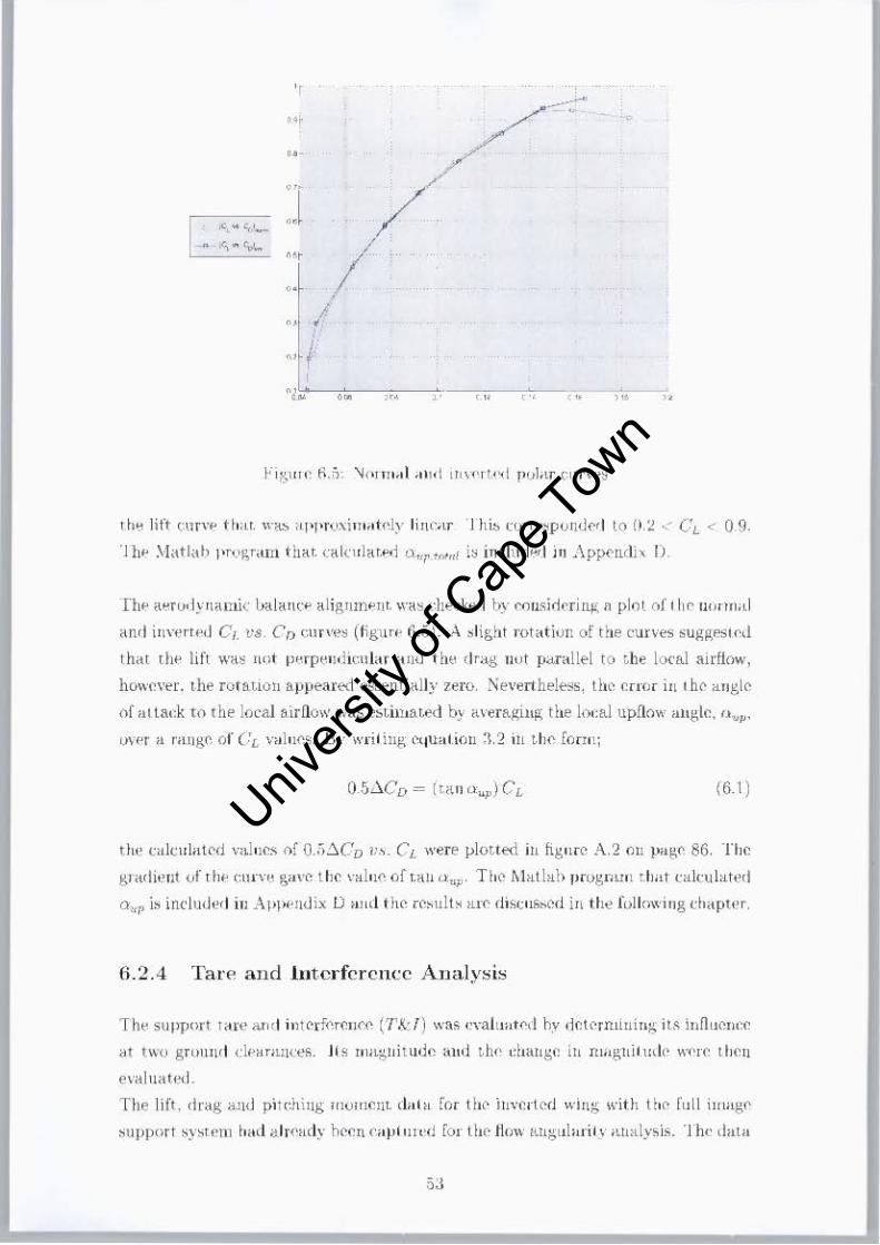
, , ~ -.. "
u
"',~~'-::I
-. "0, ~ 'oJ.. "r
,.
0.' I " I " ,. o. " , " "
,. ,.
lh~ lit't C\1F~ tlo:l!. ".~ "pp r('.xim.,Wly linr.lr I hb nJrre:;p<Jlluf'd to Il.~ " CL <.0 9_
Th~ .\latlah pr('1',r,nn that. (a ku la t.PIj n"rtn',,1 i~ indlldl"'1 In .\pl-"'udh I)
fhp a~f(J' iynH mic ualancp aligllmPIlt. wa~ dw(:ked b~' NlI1s; oi~rJ n~ n pi'll of I h r IH" ",;<1
Hnd illw,rtPu CI.1'8 CD Cl1r"'-'~ (figurp 6_5) _ A ,light rotat iun of tile cunes suggesl",)
that t h!' li ft wa~ not perp tmd icl1 lar anu t he dr"", nut parallel to the local airfiow,
howc\'.,r, the rotation apveared essentia lly zero. Newnheless, the CrrOr illihe >lJlglc
of al tatk 10 t he loeal airflow was e~till1ated b} o.\'eragiug the lDl:al upfiow angle, (1",~.
O\Pf a rang" of CL valnes. JJ~' wr il ing equat ion :\.2 ill til" [Drill;
th,' calculated values of O."j.CD 11.,_ C[ were plotted ill hgnrc .11..2 on pag(' 86. The
grad ieJlt uf t h,· curve !'.m'c t he \ ~I,,(' of t. al! (~llp' T hc IIlatlab program Lha t c"kula ted
Q"P i:; includ,>d iTl .-\PP"ndD: 0 alL d thr rc,ul t" "r(' dlSC"ShCd in the foliow"lg d'aptf'r,
6 .2.4 Ta r e a nd lut crfcrcncc Analy~ i::;
Th,' su pport Wfe "",1 int ('ffNellcc (T X-J) was ",-aIL",t",1 h:.o det rrminin:,; its inflLlCnte
at t l-l'U gfOun d dpariUl(e8_ l is lIla:';l!i tude and th,' dIange in m,'gnitlJ(lr wf're then
e \'~ I u ~t<.'( I _
The lift. drag and pi tch ing mumrnt. dala [or tllr iIl'-ertcd win:,; "'ith thr fLlI I illlag('
,upport ,~,1 eIll had " If('a dy hrrn ea p i III pd [or t IIp flow IoUl:'; LlI"rit, aIml ... ·si8. The data
5J
Univers
ity of
Cap
e Tow
n

f,.r rhe "lQ~ " .. unal ami invell M """ Ih"l1 caplmed (see figure ti,v aut! 6,. ). All
1(""" ",.". rA)fidncwd ... :tll rill' " Ill;>' 1 .... 1lr<~ 1 ar till' r ",md o·o·H'l ill, · ... mllh,· gH)u",1
I,hltlt' i r~~lalll',1 -\ ,;t'CVlltl ".,.. .. r r I,,· I h".· ",,,liC,,. l<!L;"";' ... ,.$ ~u", h ... 1 ,~ I "r " gr<>II'H I
dellrdnre of /, 11iJfllfn lh" I I) rd,u ;,, ' '-0 d u' I"a,hng , 'rig" (.r Ih.· " 'lUll: In
1111 I t'SIi>. I hI' b .. h wa~ ~tM t'.m ~r\" \(. " II .. " I" L~il i""i "g of d iE' "'\I'S" ~"ppurt ~",.. ,'m
Howevtr. i" aoxurdh.nce "ita l'ufm'ri211 (~'(I ion ~ _ L" , on p«gl' 18). " ""' 111 'WIT) I.d !
WI\.' W)t ",," .. idc,-ed to be a prob]"m, ,inCl' Ct. <t: lU h o'
'I h,' lai] 'tipporr ~nu I 1" '':'1'<1 a 1'",111,' 111 f" l t h~ I.e<;: 'lJ\'ohill)l, t.lH· lIm' ~. · 'ail ~\lIIJ" "i
\ wllldshield , 1,dwfI,d p"rt "l th,' l ut l , tr l, I [W'" , I .. · "iNI,,",""'. Aq du· 'inS'" "r
IIttlick "as chan",...:!, II ... h'ngth "f 11:.· ill lii'.t' ~' n" "" ,"h~1 r,' '':'''''I!' r" ",lIIm,aln an
.... Iulll Ifoll!!,1 h of e.'l: p~ ... n.~. ,J, CO lllIX· U<o.at Itt:1 ",,,:1:0,] pl1) ]l')",,:~1 h~ Uarlvl\' ~·t al161
"al:> \I""" I III I 10,· ,, -.I ,. ·11,i.. in" .1.,-,<1 St· ~I 11.114 1 fie If'q>;l:-r ur 1!l1' ~ 1II<11'l (' 1 4 i I ~t ru t l'(I" III
I') th, ' min;""; '" I, ·o~.h <or the eAI"ll<'<i tll,l stru t (.'io.'" fi)(lIre 61S)_ for 0:'4ch 11['1:;11'
(.f 8ttark, til(' d,~ "m' "''''"1'1.11 !-tell" ;" !<'(i hy '1\0' miS!>i ,, ~ ,m!>'.!;" ,wi S("ClivlI lilt.
,.,.till,aI":] and api'h",\ W II", ~ ~ t8.
rh ~ add it iowl.l tail 'U]Jpor t drag \\'H~ I"-",I" ... ,,,,j Il\' pln t. ting 11", drag """in" rlw
'·X I"",,·t! kll1\lh uf (he 1Il ~ 1!l ~t rn t~ (,itlr(' ... 11 ~trUl ~ ""r!' id,'ulim lj Sin",· dnog i~
Univers
ity of
Cap
e Tow
n

T sl mtn
T sUm"9"
'.
Figure 5.S. Lengt h uf image jail strut
J5
Univers
ity of
Cap
e Tow
n

Fi;;UfP G.O Addil10nal kn~th v,d(h l to lllW!j" Lail "til"
pmjJ"rt 1011a1 t 0 arpa, a Ii W','T (urw ".,,,~ ~xJl~(l.l'd, Tht ktlgt h of til" "".,-,111); """';, JIj
('Ill the illlnpT strut w~, cakulatrd as n fnnctwTl of aag i,' or atl<,d., (,,'.' fi~ur~ 6,0),
J I,,· addJllOl1~.l drag rOlllj)l']wnt wa~ t hru cak1 11~vd ;h" r",wl ion vi ,. Th~ H'''HH'll'
t'.,·,,,·t;J.u'd b,1" Ihr addi"onll.] d ,ng COlllpOlwut ,,"':' "~' '' TLaL<-d hI" "pl'l~'illg th" fllr('~ at
Ih" erll1l'<' of Ihe Hb~ .. ll1 s,'ctioll (se,' figure (UO), T ins ,JO(JI,u'nt "'Cl' ("kH]<tt~d for
,-adL val U~ of (). All imag'" I ail ,Lt HI, tolll lH'n:>Jl! ion "~,, appli.~d to th~ data from th~
in,en,.d t~'1 ",ilh th,' full illJa&,' "[1'1>011. ,-,"St""L '1 h" additillildl tail ,uPI-'0rt drag
ami lllll'OIrllt t~blr' ar~ ill('.h~l,'d in '\p!-,,'Illlix L
n,'fore the T&I fllm'eli"ll ! erm~ for each angle 01' attack conld b e sohed [or, Ihe
d»ta from "lllhn~ ' t "sts was fir~t cornX'ted for thr \'ariatjon in weigh! I.au'. OW'" aC-
1'0lmh'd for_ t h, ' con"ctioll 1c'rms \\',,[0' del ennined b,i ,nbl.raer.in.:-; 1.h,. win~ lll\,,.ll,,.d
data f'rolll th~ wiltg iu\"C'u"d "~1.h [tli] imag,. 'UPP(!Tt '.'Stl"tL Thi~ "'ClS giwn by:
D"" ,
[Lim, + [rk;]]"r_£. -+- -T~rlo", [~ - L,n" + T~1imd.J [T&IJ"" L
[D"", i [Tkl l~rD + [T&F1oo}DI
[T!::ILrD
1.11,,,. 1- TA.-11"~M + T&lll<,,;JI[ -1.H,n. -+- T,k(lo,,· .\I1
[T&J]"p-'f
Tb.,' e()rr"CI.ioll WllI1~ arr illcluded in Appuldix E. which im'lude:, thl' ("()rrr('!ion
t,']'jllS calculalrd ht Ihr tlllmrl (·entrrline. at a gr01llld ciearallcP 01' II = 220mm
,'j(j
Univers
ity of
Cap
e Tow
n

I
II \
M>T'~ ~ - ------- -- -- -- - _ D ,r"
(hn ,j ) ~I"l I ll<' ""'"11 ,;1.j,ws of r.hi- I" ,", Tlw T ~Sll lts (,f ,h" T& / ~JL"I ,\"i" an'
d"""_,,,, ) 'ro ill(' fnllowII lli ' h ~l'tPl .
(i.J Test Procedure
6.3. L Preparation
Ouce t he TNl aad weight tare tests wt'r~ cumpleted, t he wiug was l>o,itiolled ill
lht' Borm,,\ clJ1lfir,maliolJ The transducers readlllr," werr Lerocd aud rrJl<'at~bil i ly
clll'ck~d OflU' agaill For ('aclL cOll>pOurlll. of hit, d rag ""d pll.dl1['g lIlomt'ni , a 2-D
llHurix was construckd ill Exct'i T ht· hm;~()utal axb (columll~) represented the
,,"r,lc of all.ack and t he vertical axi, (row~) r~prl':,~ntt>d the ground clearance. The
""file of attack "as varied frum -10 to 36", in 'r increments Thus. 2·1 separate
"llgll"S \"~rr I c~t""L "lht' IiIO,md c1earauce "as ,-aried ["'Jm 2'){}mm. (/1{) = 1.80)
dOlo1.11 to 10 mm (h o = (Hlb)_ Th~ iIlOt'IllPJL h iJL grouud (l€ar~.IlC€ \-ari€d. but b€low
Hi1 "1m {"o = 1) the gTOUllli riear;""'t' w,,~ {'hangpd ill IOmm illnemem~. Tl'St~
WO'[e carried ou t at a total of 20 '""pan.1(> gruuJLd ( l€ara IlC€~ Thus. ~ach 20 x 24
matrix CO[l> l ,;v~1 of 180 UIIJLl"" 1,,_1 ( 'ollligumlioll~ ba",d 011 r\[l~lr of al lack alld
grou JLd cI ~a.ra 1l ct' .
, .• ' ,
I
Univers
ity of
Cap
e Tow
n

Table 6.1: Test Conditions
Inclined Manometer Reading 120.0 mm Dynamic Pressure, q 242.4 Pa
Velocity 20.1 m/s Velocity 72.5 km/h
Mach Number 0.06 -
Effective Reynolds Number, Reeff 2.21 x 10⁵ -Cylinder Rotational Rate, N 1373 rpm
6.3.2 Testing
The ground clearance was measured vertically from the trailing edge of the wing to
the surface of the belt (figure 2.1 on page 7). For each angle of attack, a marker
on the balance elevator system indicated the ground clearance on a scale rule. The
angle of attack was set and the data captured at each specified ground clearance.
When all ground clearances had been tested, the angle of attack was changed and
the procedure repeated. The uncorrected data for the lift, drag and pitching moment
is included in Appendix E. However, sixty one combinations of ground clearance
and angle of attack were impossible to test at due to physical limitations of the
wing support system and balance elevator system. These included; negative angles
of attack at very low ground clearances, high angles of attack at very low ground
clearances, and, medium to high angles of attack at high ground clearances.
For all test runs, the velocity of the airstream was maintained at 20 m/ s. This
corresponded to a dynamic pressure, q = 242 Pa, which was measured using an
inclined manometer and a pitot-static tube. From the airstream velocity, the re
quired rotational speed of the rolling cylinders was calculated. This matched the
belt velocity to the airstream velocity. Table 6.1 indicates these and several other
variables relating to the test conditions.
6.4 Post-Test Procedure
6.4.1 Initial Corrections
The data was then corrected as previously specified. An overview of these corrections
details the following adjustments to the recorded lift, drag and pitching moment;
l. Lift
(a) T &I correction
58
Univers
ity of
Cap
e Tow
n

(b) Correction to angle of attack
2. Drag
( a) T &1 correction
(b) Drag increment due to aerodynamic balance misalignment
(c) Correction to angle of attack
3. Pitching Moment
(a) T &1 correction
(b) Weight tare correction
The individual corrections and the corrected data are included in Appendix E.
6.4.2 Final Corrections
The final correction was made to the dynamic pressure, q. This was achieved through
the solid and wake blockage correction terms. Blockage normally applies to every
thing in the test-section. This includes the wing support system, the windshields
or any other items required in the test-section during the test. However, since the
image method was used to evaluate the T&I, the blockage due to the wing sup
port system and windshields was accounted for. The solid and wake blockage was
accounted for as follows.
Solid Blockage
The solid blockage correction factor was constant with angle of attack and ground
clearance. The solid blockage was calculated using figure 3.8 on page 28 and fig
ure 3.9 on page 29. The required parameters are listed below.
Table 6.2: Solid Blockage Calculation Parameters
Wing Thickness Ratio, tic 0.143 -
Span-to-Tunnel Breadth Ratio, biB 0.53 -
Tunnel Aspect Ratio, B I H 1.55 -
Estimated Wing Volume, Volwing 0.0012 m3
Test-Section Area, C 0.453 m2
The wing volume was estimated using equation 3.12. From figure 3.8, the body
shape factor, K 1 , was estimated using the curve of the 4-digit N ACA profile. The
59
Univers
ity of
Cap
e Tow
n

tunnel-model shape factor, Tl, was estimated from figure 3.9. Both values are listed
below.
Table 6.3: Estimated Values of Kl and Tl
Body Shape Factor, Kl 1.03 Tunnel Shape Factor, Tl 0.875
The open test-section solid blockage was given by:
Esb.open
Wake Blockage
-0.25Kl Tl V olwing C1.5
-0.00089
-
-
(6.2)
The wake blockage correction factor varied with angle of attack and ground clear
ance. The wake blockage terms, CDO and CDS, were determined using the following
method. For angles of attack below the stall angle, the total drag coefficient was
divided into parasite and induced parts;
CD C2
CD.Pe + ~R ?r.e. (6.3)
CD .Pe + K.cI CD .Pe + CDi
Where;
• CD .Pe - equivalent parasite drag coefficient
• K = l/?r.e.AR
• e - span efficiency factor
• AR -=- aspect ratio
Parasite drag (CD .P ) is assumed constant with angle of attack; and includes skin
friction drag, pressure drag and drag due to interference, excrescences and rough
ness. For a wing, CDO is essentially the same as the CD .P ' The product of the span
efficiency factor and the aspect ratio, e.AR, represents the effective aspect ratio of
an equivalent wing having an elliptical lift distribution. The value of e is usually
close to, but less than, one. The value of e usually decreases with decreasing AR,
but in ground effect e can increase to values greater than one.
60
Univers
ity of
Cap
e Tow
n

A value for K and CD .Pe were required for each value of ho. The value of K and
CD .Pe were determined from a plot of CD vs. CI from the data at each ground
clearance[6]. For 0.2 < CL < 0.9, each curve was approximated as linear. The gra
dient of the linear curve was set equal to K. Finding K meant e could be calculated
as well. CD .Pe , an approximation to the true parasite drag, CD .P , was given by the
intercept of the linear curve with the CD axis. For each value of ho, C DO was set
equal to C D .pe . CDS was then calculated over the full range of ho and D values,
given by;
CDS CD - C Di - C DO
CD - K.C't - CD .Pe
In calculating CDS, if the value became negative, the flow was considered unsepa
rated, and the value of CDS set to zero. The values of e, the wake blockage correction
factor and the final corrected dynamic pressure are included in Appendix E and dis
cussed in the following chapter. No further corrections were required. All that
remained was to transfer the moment data to a desired centre-of-gravity location
and reduce the force and moment data to coefficient form with the corrected dynamic
pressure data.
6.4.3 Moment Transfer
The pitching moment was measured about the trunnion of the main support struts.
This represented the balance moment centre. However, the moment is usually trans
ferred to a desired centre-of-gravity location on the model, usually the 1/4MAC.
With reference to figure 6.11, this was achieved as follows:
R
'P
Ml/4MAC
arctan (f) Jy2 +X2
E+D
MtT + L.R. cos 'P + D.Rsin 'P
MtT represents the moment measured about the balance moment centre (the trun
nion). The values of X and Y were known from the model (wing) making process.
Thus, 'P, and hence Ml/4MAC, was calculated as a function of D. The process was
repeated for each data set corresponding to a different value of ho. It was important
that all corrections, weight tares etc, were applied before the moments were trans-
61
Univers
ity of
Cap
e Tow
n

- R
. -y.
~-- --
6.4.'1 Resol utio n of t llf' A('I'odyna nlit: Centre in Pil Ch
Ttw rf'!IOhl t h ,11 " f t h.' I"""il iOIl or I h,' 1t" ,00..-lIa1l1'" ,,..." t~, · ill 1-"t..R (ACP), rur ~ ... n~Ulnt
,.,.hu,," ur !Ia, "''-''~ ~,.,.~ "a~ro u('.'<t. T it .. ('" I <. C~ dl!.\a ""'n 1)la fh." '- " furKli(J!l uf
a n it' ('If dl<t.a "'Ii., glW,. rt ..... " '·'· t il I )", 1, ~\IAC Body-lixt'd ues W~IE' dehnM.
[1'1(\11\'''''' thi, I-'"im. and wen' "I iglh~ ! fLJlw 1l.rd , ~tarlJOard. (\mj duwn (see fij(u",
L~). From E-qu3tiDIl 1X t he ACr Wll9 ctdine,l by:
x"
1 h('T(.fort'. lh" ~h ll'" <lr th,- c", l'~ CL d~':t IV" '- tit,· d i, t,..",x· '" th" ,\ C P. X. ,. ,,, a
fmlt'Hull of" Il",,',nn. it w~, d''',:id,'(f W I lad, th~ ACP as til" wil1)1, "lI t"I"! Io:TP""d
df" ,t. bv r"",,1 " ing tbe fUll''''' Hml 1IIllUH' l l t.s ", p;i, "II by equatiull 2 11 . l~-" I .U' 'II IWr"
Univers
ity of
Cap
e Tow
n

for convenience.
0= OCM .Ref
oCL
-- 1 + CD-- cos a + -- - CL-- sina X [( oa ) (oC D oa ) 1 c oCL oCL oCL
-- CL-- - -- cos a + 1 + CD-- sina Z [( oa oC D) ( oa ) 1 c oCL oCL oCL
Solving this equation would allow the movement of the ACP along the chordline
and above/below the chordline to be tracked as the wing entered ground effect. The
data was used to find CL , CD and a, and, linearised over the region 0.45 < CL < 0.9
to find the slopes of OCM/OCL and oa/oCL . The data was linearised over this
region since it corresponded to 3 < a < 11, which were the expected cruise angles
for normal flight. Since the value of the span efficiency factor, e, had already been
calculated, the value of OCD/OCL was found from the derivative of equation 6.3;
The substitution of the data, from two points/angles in the linearised region, allowed
the simultaneous solution of equation 2.11. The program that performs each of these
tasks was included in Appendix D and the results are discussed in the following
chapter.
6.4.5 Resolution of the Aerodynamic Centre in Height
The resolution of the position of the aerodynamic centre in height (ACH), for con
stant values of a, was evaluated as follows. The CM vs. CL data was plotted as a
function of ho. Once again, the CM data was given relative to the 1/4MAC. Body
fixed axes were defined relative to this point, and were aligned forward, starboard,
and down. The calculation of the ACH was made utilising equation 2.12, namely;
63
Univers
ity of
Cap
e Tow
n

Therefore, the slope of the curves gave the distance, in percentage chord, to the
location of the ACH, as a function of ho (0: - constant). However, the resolution of
the ACH by equation 2.12 was limited in that it only defined the movement of ACH
along the chordline (assuming the moment axis lay on the chordline). A curve fit of
the CL vs. ho and CM vs. ho data was made using a Matlab smoothing spline for
0: = [3, 5, 7, 9, 11]. The smoothing spline from the Matlab Curve Fitting Toolbox
was found to give the best fit of the curves. Furthermore, the toolbox allowed
immediate computation of the derivatives of each curve. From this data, the ACH
was calculated. The results are discussed in the following chapter.
64
Univers
ity of
Cap
e Tow
n

Chapter 7
Test Results
The force and moment data from the experiments is presented in Appendix E,
and the various plots of the data included in Appendix A. This includes data
from the pre-test procedures. Based on this data, the observations, interpretation
and discussion of the results is made in this chapter. The test correction data is
analysed first. This is the data used to correct the lift, drag and pitching moment.
The corrected lift, drag and pitching moment data is then analysed, followed by
the resolution of the aerodynamic centres in pitch and height for an analysis of the
static pitch stability.
7.1 Test Correction Data
7.1.1 Aerodynamic Balance Alignment
The aerodynamic balance alignment was determined by running the wing with the
full image support system (figure 6.3), in both the normal and inverted configura
tion. The wing was positioned at the tunnel centreline and pitched from -10 to 36°.
The normal and inverted curves of CL VS. Q: (figure 6.4 on page 52) suggested
Q:up.total was large. The analysis yielded a total angle correction of Q:up.total = 1.05°.
Therefore, the indicated angle of attack was 1.05° too low.
The normal and inverted curves of CL VS. CD (figure 6.5 on page 53) illustrate
good alignment of the lift and drag vectors relative to the mean airstream. The
analysis yielded a local upflow angle, Q:up = 0.12°. Therefore, the flow angularity
was up, increasing the angle of attack by 0.12°. This error was of the order of the
error in aligning the balance, wing support structure, etc. l!pflow was therefore
considered negligible, as suggested by the curves.
65
Univers
ity of
Cap
e Tow
n

7.1.2 Tare and Interference
The support tare and interference (T&I) was evaluated by determining its influence
at two ground clearances. This included the tunnel centreline (h = 275 mm) and
h = 220 mm. From the lift and pitching moment T&1 curves; the magnitude of
the T&1 corrections were of the order of the accuracy of the balance transducers
at low to medium angles of attack (figure A.3 on page 87). At high angles of at
tack, the curves illustrate more significant corrections are required. The lift and
pitching moment corrections changed in sign several times with increasing angle of
attack. The drag T &1 curves indicate the correction was more significant, with the
correction an order of magnitude higher than the accuracy of the transducers. The
drag correction remained positive, except at very high angles of attack, where it
became negative. Figure A.3 clearly illustrates regions in the T&1 curves in which
the correction varied with ground clearance.
Although the T&1 corrections had changed with varying ground clearance, since
the T &1 analysis was only conducted at two elevation levels, the mean T &1 correc
tion values were applied to all subsequent test data.
7.1.3 Boundary Corrections
The results of the boundary corrections are given in figure A.4 on page 88. This
figure shows the total blockage correction factor, Etotal, as a function of angle of
attack, at different values of ho. The curves indicate that the error in the airstream
velocity due to solid and wake blockage was less than 0.5% below the stall angle
(approximately 19°). Furthermore, for -5 < ex < 11 degrees, Etotal remained ap
proximately constant with ex and ho. The error in the airstream velocity, above
the stall angle, increased almost linearly with angle of attack, from 0.5% at stall to
approximately 3% at 37°. The maximum error in the airstream velocity was esti
mated to be 3.4%, which corresponded to an angle of attack of 37° and a ground
clearance of ho = 0.12. Furthermore, the curves suggest the blockage increases with
decreasing ground clearance. A plot of the span efficiency factor, e, indicated a
significant increase in the effective aspect ratio (e.AR) as the wing approached the
ground (figure A.5 on page 89).
66
Univers
ity of
Cap
e Tow
n

7.2 Force and Moment Data
7.2.1 Lift Coefficient, CL
The CL data is plotted in figure A.6 on page 90 as a function of a and ho. The
following observations are made.
• The data indicates that a reduction in ho causes an increase in CL for a > 0°.
The CL at a = 0° is approximately the same for all values of ho. Negative
angles of attack show a decrease in CL for a reduction in ho. The lift curve
slope, (oCLI oa )0.=0' increases as the ground is approached. The angle of zero
lift, aLD, increases from a = -4.2° to a = -1.6°, however, this change is small
for ho > 0.43.
• The CL .max increases with decreasing ground clearance, coupled with an in
crease in the stall angle. The CL at stall and ho = 0.06 is approximately 21 %
higher than that at ho = 1.8. The average stall angle occurs at a = 19°. The
maximum stall angle occurs at a = 23° for 0.12 < ho < 0.19. However, for
ho = 0.06 the stall angle is not reached.
• The minimum loss in lift at stall is 4% at ho = 0.12. The maximum loss in lift
at stall is 18% at ho = 1.18.
• For angles of attack greater than the stall angle, the CL increases significantly
as the ground is approached. The highest recorded increase in CL is 38% at
ho = 0.06, a = 23°. Furthermore, for 0.12 < ho < 0.5 the CL.max does not
occur at the stall angle, but at the maximum measured value of a (= 37°).
• For positive angles of attack below the stall angle, the data indicates the
slopes of the CL VS. ho curves change from negative to approximately zero
(some positive) over the region 0.25 < ho < 0.5. At approximately ho = 0.25,
a further reduction in ho causes as significant increase in CL and the slope
becomes negative again.
Discussion: The data indicates that a reduction in height causes a loss in lift at
negative angles of attack, little or no change at zero angle of attack, and an increase
in lift at positive angles of attack. The increase in aLO is as a result of the increase
in the lift curve slope, (oCLloa)o.=o. These results correlate well with the results of
Fink and Lastinger[18], and, Serebrisky and Biachuev[17]. Furthermore, the highest
recorded increase in the CL is 38% at ho = 0.06, a = 23°. This compares well with
figures quoted in the literature[4]. At ho = 1.06, the curve representing a = 21°
indicates an abrupt lowering in the CL as a result of the lower stall angle.
67
Univers
ity of
Cap
e Tow
n

The CL .max at stall remains approximately constant as the ground is approached.
However, for ho < 0.43 the maximum lift coefficient increases significantly with
decreasing ground clearance. For ho < 0.37, there is a significant increase in the
stall angle. In contrast, Serebrisky and Biachuev[17J found a reduction in the stall
angle as the ground was approached. However, the decreasing severity of the stall
agrees well with the results of Serebrisky and Biachuev. There is insufficient data to
examine the stall pattern below ho = 0.12, however, it appears the wing may even
tually cease to stall at these high angles of attack and very low ground clearances.
Rozhdestvensky[2J classifies ground clearances of ho < 0.1 as extreme ground effect.
Under these conditions the airflow can stagnate. Since the airflow over the upper
surface of the wing is fully separated at these high angles of attack, the source of
the additional lift, which prevents the wing from stalling, is thought to be due to a
large stagnation pressure on the lower surface of the wing.
For several positive angles of attack, there is a small loss in lift for 0.25 < ho < 0.5.
Serebrisky and Biachuevl17J describe this trend of the CL as a result of a simulta
neous increase in the pressure on the lower surface of the wing, and, a decrease in
pressure on the upper surface, near the leading edge, as the ground is approached.
This produces an increase in the unfavourable pressure gradient on the upper sur
face, which results in early flow separation. At larger ground clearances, the increase
in pressure on the lower surface can be insufficient to compensate for the loss in lift
due to early flow separation. This can result in a lower CL relative to that when the
wing is in free air. The plot of CL vs. ho clearly shows this loss if CL at ho = 0.5
for -1 < a < 7. At smaller ground clearances, the increase in pressure on the lower
surface is increasingly more than the increase in pressure on the upper surface due
to early flow separation. This results in an increase in the lift coefficient, at small
ground clearances, above the free air maximum lift coefficient. This is visible in the
plot of CL vs. ho for a > 10, ho < 0.25.
The change in the slope of CL vs. ho affect the first requirement for the wing to be
stable in height. At positive angles of attack, the CL increases with decreasing ho.
Therefore, the slope of the curve, aCLI aho, is negative and the wing is provision
ally stable in height. However, for positive angles of attack below the stall angle,
the data indicates a transition of the slope from negative to approximately zero
(some positive) over the region 0.25 < ho < 0.5. In these regions the wing becomes
marginally stable (or unstable) in height. At negative angles of attack, there is a
decrease in the CL with decreasing ho. The slope of the curve is positive and the
wing is thus unstable in height.
68
Univers
ity of
Cap
e Tow
n

7.2.2 Drag Coefficient, CD
The CD data is plotted in figure A.7 on page 91 as a function of a and ho. The
following observations are made.
• The minimum drag coefficient, CD .min , occurs at approximately a = _3° for
ho > 0.31. For ho < 0.31, CD .min occurs at approximately a = -1°. CD .min
increases from CD = 0.023 at ho = 1.8, to CD = 0.043 at ho = 0.06.
• The data indicates a reduction in CD with decreasing ho, for aLO < a < 15
degrees.
• For a > 15°, the CD increases as the ground is approached.
• The CD increases by an average of 75% after passing through the stall angle.
The smallest increase in drag is approximately 50%, which occurs at ho = 1.06.
The largest increase in CD is approximately 100%, which occurs at ho = 0.06.
• Above the stall angle, the CD increases by up to 46% with decreasing ho.
Discussion The value of CD .min occurs at low (zero) values of CL and is usually
assumed equal to the profile drag, CDO ' CDO is a function of skin friction drag and
form drag, which are functions of the profile of the wing, hence the name, profile
drag. Furthermore, CDO is ideally independent of AR.
Acknowledging that the tests were conducted at different Reynolds numbers, the
values of CD .min are of similar magnitude to the results of Zimmermanl24]' and, Fink
and Lastingerl18], but greater than those of Serebrisky and Biachuevl17]. Since the
wing profile used by Zimmerman is similar to the one used in these experiments,
this may explain why the results are similar. However, the profile used by Fink and
Lastinger is a substantially thicker (22% thickness ratio) profile. Yet, the values
of CD .min are almost identical. The profile used by Serebrisky and Biachuev is a
slender 12% thickness ratio wing, but does not have a flat bottom. The CD .min val
ues measured by Serebrisky and Biachuev are approximately half that measured in
these experiments. The primary reason for the contrasting CD .min values is thought
to be due to a combination of the elevated rear flap on the wing used in these exper
iments, and, differing test Reynolds numbers. All three wings from references [[17],
[18], [24]], are highly streamlined toward the trailing edge and are tested at higher
Reynolds numbers.
Below the stall angle, there is a general lowering of the CD with decreasing ho.
This agrees well with the results of all the references listed above. Serebrisky and
69
Univers
ity of
Cap
e Tow
n

Biachuev (AR = 5) and the larger AR wings (AR > 4) used by Fink and Lastinger
present the most significant reduction in CD near the stall angle. The larger aspect
ratios are thought to be the primary reason for the greater reduction in CD, at higher
angles of attack, through a greater reduction in the CDi . This is in good agreement
with general ground effect theory, which predicts a reduction in induced drag[4, 1].
7.2.3 Moment Coefficient, CM
The CM data is plotted in figure A.8 on page 92 as a function of Q: and ho. The CM
is given relative to the 1/4MAC. The following observations are made.
• For 3 < Q: < 11 degrees, the slope of the CM vs. Q: curves is positive.
• For -7 < Q: < 17 degrees, the slope of the CM vs. ho curves is approximately
zero for ho > 0.5. For ho < 0.5, the slope of the curves becomes negative.
• For Q: > 19°, the CM decreases significantly with decreasing ho. The large
positive slope of the CM vs. ho curves is in agreement with this.
Discussion For 3 < Q: < 11 degrees, the CM is not constant with Q: as identified
by the positive slope. Therefore, the ACP cannot be located near the 1/ 4MAC as
stated by ideal aerodynamic theory[25]. Judging by the large positive slope, the
ACP is suspected to be forward of the 1/4MAC. However, the CM is constant with
ho for ho > 0.5. This suggests the ACH is located at or near the 1/4MAC.
The nature of the CM curves agrees well with the data and explanation of the
flow field given by Serebrisky and Biachuev[17J. At larger ground clearances, the
early flow separation caused by the increased adverse pressure gradient, result.s in
an increase in pressure on the rear half of the upper surface of the wing. This causes
an increase in CM with decreasing ho, as seen in this experiment for 3 < Q: < 11
degrees . .:\ear the stall angle, separation occurs close to the nose of the wing. This
causes an increase in pressure in front of the moment axis (1/4 MAC), which results
in a net decrease in the pitching moment, as seen in this experiment Q: > 13°.
7.2.4 Polar Diagrams
The CL VS. CD data is plotted in figure A.9 on page 93 as a function of ho. The
CL vs. CM data is included at this point for completeness; however, it is re-plotted
and discussed in the analysis of the aerodynamic centre in pitch (section 7.3.1). CM
70
Univers
ity of
Cap
e Tow
n

is given relative to the 1/4MAC. The following observations are made regarding the
drag polar data.
• Considering the curves along constant lines of C L, the following trends are
noted. At negative values of CL there is a reduction in CD, with decreasing
ho. At approximately CL = -0.1, CD = -0.05, CL and CD remain approxi
mately constant for all values of ho. For -0.1 < CL < 0.4, CD increases with
decreasing ho. CD .min occurs at approximately CL = O. At approximately
CL = 0.4, CD = -0.05, CL and CD remain roughly constant for all values of
ho. For 0.4 < CL < 1, a reduction in ho results in a reduction in CD'
• The maximum lift coefficient before stall increases from CL = 0.98 at ho = 1.3,
to CL = 1.14 at ho = 0.12. However, the drag simultaneously increases from
CD = 0.2, to CD = 0.44. There is insufficient data on the stall characteristics
at ho = 0.06.
• The minimum loss in lift at stall is 4% at ho = 0.12. The maximum loss in lift
at stall is 18% at ho = 1.18. Following stall, there is a marginal increase in CL
at constant values of ho. However, the CD increases by an average of 40%.
Discussion The minimum drag coefficient, CD .min , occurs at approximately CL = O. This agrees with basic aerodynamic theory[25] and with the results of Serebrisky
and Biachuev[17]' and, Fink and Lastinger[18]. Furthermore, for -0.1 < CL < 0.4,
CD increases with decreasing ho. Over this region, CD is primarily due to skin
friction and form drag, which suggests a net increase in these two effects as the
ground is approached. At CL = 0.4, CD = -0.05, CL and CD remain approximately
constant for all values of ho. For CL > 0.4, the increased efficiency of ground effect
is demonstrated by an increase in the slope of the CL VS. CD curves as the ground is
approached. Furthermore, CL .max at stall clearly increases with decreasing ground
clearance. However, the CD at stall is seen to simultaneously increase under these
conditions, and the efficiency of the wing rapidly deteriorates. In contrast with
Serebrisky and Biachuev, the CL .max at stall also increased with decreasing ground
clearance, however, they found CD decreased at stall. The plot further illustrates
the ability of the wing to maintain high values of CL after stall. This is particularly
so for ho < 0.25. However, the high values of CD would make it highly impractical
to operate the wing under these conditions.
7.2.5 Lift/Drag Ratio
The L/ D ratio data is plotted in figure A.10 on page 94 as a function of CL and ho.
The following observations are made.
71
Univers
ity of
Cap
e Tow
n

• At ho = 1.55, the maximum L/ D ratio, L/ Dmax = 9.7 at CL = 0.44 (0: = 3°).
• At ho = 0.06, L/ Dmax = 13.1 occurs at CL = 0.75 (0: = 5°). This is the
highest L/ D ratio of the test.
• The lowest value of L/ Dmax = 8.5 at CL = 0.62, ho = 0.62.
• For CL < 0.4, L/ D decreases with decreasing ho. The plot of L/ D vs. ho, for
0: < 3°, shows a further decrease in L/ D with decreasing ho.
• For 0.8 < CL < CL .max at stall, L/ D increases with decreasing ho. This
corresponds to 7 < 0: < 19.
• An increase in CL (0:) from L/ Dmax to the CL .max before stall, indicates the
L/ D ratio drops by approximately 50% at ho = 1.55 and 80% at ho = 0.06.
• For 0: > 23°, L/ D decreases with 0:, but remains constant with ho.
• The lowest value of L/ D = 1.4 (for CL > 0) occurs at 0: = 37° for all values
of ho.
Discussion The data indicates a 35% increase in L/ Dmax for a reduction in ground
clearance from ho = 1.55 to ho = 0.06. The corresponding angle of attack increased
from 0: = 3° to 0: = 5°. However, as the ground clearance was reduced, L/ Dmax
first decreased, before increasing again to reach the maximum L / D ratio of the
test. The L/ Dmax of the test was 13.1 for a lift coefficient of CL = 0.75. In
comparison with the wing of AR 2 used by Fink and Lastinger[18]' at the same
ground clearance, the L/ Dmax = 17 was produced at CL = 1.1. The wing of AR 4
produced a L/ Dmax = 35 at CL = 1.5. However, the corresponding L/ Dmax is
similar in magnitude when out of ground effect. It is clear from these tests that
both an increased AR and a decrease in ground clearance, significantly improve the
L / Dmax of the wing.
7.3 Aerodynamic Centres
7.3.1 Aerodynamic Centre in Pitch
The resolution of the positioIl of the aerodynamic centre in pitch (ACP), for constant
values of ho, is presented in this section. The CM vs. CL data is plotted in figure A.ll
on page 95 as a function of 0:. CM is given relative to the 1/4MAC. Body-fixed
axes are defined relative to this point, and are aligned forward, starboard, and
down (figure 2.8). The region of interest on this curve is that corresponding to
72
Univers
ity of
Cap
e Tow
n

o < 0: < O:stall. This represents the limits of the expected flight cruise angles. The
following observations are made .
• For 0.2 < CL < 0.45, the slope of the curves is approximately zero, except
for ho = 0.06 and ho > 0.43. Over these regions the slope is predominantly
negative .
• For 0.45 < CL < 0.9, the slope of the curves is positive. At ho = 0.06, the
slope of the curve is both positive and negative.
Discussion As specified by equation 2.8, the slope of the curves gives the dis
tance to the location of the ACP as a function of 0:, for constant values of ho.
The distance is given in percentage chord and is relative to the moment axis. For
0.2 < CL < 0.45 and ho < 0.43, the horizontal slope indicates the CM is approxi
mately constant with CL . Therefore, the position of the ACP is approximately at
the 1/ 4MAC at these lower ground clearances. For ho > 0.43, the slope is negative,
therefore, the ACP must lie backward (i.e. toward the trailing edge) of the 1/ 4MAC.
For 0.45 < CL < 0.9, with the exception of ho = 0.06, the slope of the curves is
positive. Therefore, the ACP must lie somewhere forward of the 1 / 4~AC. The slope
decreases with decreasing ho, therefore, the ACP must approach the 1/4MAC with
decreasing ho.
It was decided to track the ACP, as the wing entered ground effect, by resolv
ing the forces and moments as given by equation 2.11. Solving this equation would
allow the movement of the ACP along the chord and above/below the chord to be
tracked. The data was linearised over the region 0.45 < CL < 0.9, corresponding
to 3 < 0: < 11 degrees, and the results of the determination of the ACP, over this
region, are illustrated in figure A.12 on page 96. The x/c position of the ACP is
given relative to the leading edge (LE) of the wing with positive being backward.
The positive direction of z / c is down. The results indicate that the position of the
ACP essentially remains at x/c = 0.18 for ho > 0.5. For ho < 0.5 the ACP moves
toward the trailing edge (TE). At ho = 0.06 the ACP is located at approximately
x/c = 0.25. This trend of the ACP moving toward the TE, at low ground clear
ances, is in good agreement with Rozhdestvensky[2]. The wing used in his analysis
is a 2-D N ACA - 0008 profile with a flat lower surface and a lower trailing edge
spoiler. His analysis shows the movement of the ACP as a function of the param
eter ({}/ho). Choosing {} = 3°, several values of Xa are plotted in figure A.12. The
results show the ACP is initially close to the chord line and moves down with de
creasing ho. At low ground clearances the ACP moves back toward the chordline.
At ho = 1.3 the ACP is located at z/c = -0.002. The greatest deviation below the
chordline is z/c = -0.006 and occurs at ho = 0.5. At ho = 0.06 the ACP is located
73
Univers
ity of
Cap
e Tow
n

at z / c = -0.0003. This indicates the vertical position of the ACP is essentially
uninfluenced by the presence of the ground, and, assuming it to lie on the chordline,
is a good approximation for this wing.
The moment data was transferred to the location of the ACP corresponding to
each value of ho. The results in figure A.12 clearly show the pitching moment is
approximately constant for 5 < a < 11 degrees and all values of ho.
7.3.2 Aerodynamic Centre in Height
The resolution of the position of the aerodynamic centre in height (ACH), for con
stant values of a, is presented in this section. The CM vs. CL data is plotted in
figure A.13 on page 97 as a function of ho. CM is given relative to the 1/4MAC.
The region of the curve of interest is that corresponding to 0 < a < astall' This
represents the limits of the expected flight cruise angles. The following observations
are made.
• For 3 < a < 11 degrees, the data illustrates the curves form an '5' shape .
• For 11 < a < 19 degrees, the data illustrates the curves form an inverted 'V'
shape.
Discussion As specified by equation 2.12, the slope of the curves gives the distance
to the location of the ACH as a function of ho, for constant values of a. The distance
is expressed in percentage chord and relative to the moment axis. For 3 < a < 11
the 5-shape means the curve has positive and negative infinite gradients. Therefore,
X h is expected to take on infinite positive and negative values. This immediately
breaks the condition for static stability as defined by equation 2.20. The shape of
the curves, for these values of a, corne as a direct result of a small loss in lift at
ho = 0.5 (figure A.6). This was identified as a failure of the first condition for static
height stability, oCL/oho < 0 (equation 2.17), and, illustrates how X h is affected
by a failure to meet this condition. For 11 < a < 19 degrees, the curves illustrate
large positive and negative gradients. Therefore, X h is expected to move forward
and backward from the 1/4MAC.
The position of the ACH, as a function of ho, was calculated as specified by equation
2.12. This tracked the movement of the ACH along the chordline. A curve fit of
the CL vs. ho and CM vs. ho data was made for a = 3, 5, 7, 9, 11 degrees. The
derivative of each curve was made in Matlab (figure A.14 on page 98). oCL/aho clearly takes on positive values for 0.2 < ho < 0.5, thus violating the first condition
74
Univers
ity of
Cap
e Tow
n

for static height stability (equation 2.17). From this data, the ACH was calculated.
The results are presented in figure A.15 on page 99. The xlc position is given rel
ative to the leading edge (LE) of the wing with positive backward. Included in the
figure is the position of the ACP for each corresponding value of ho. For ho > 0.5,
the figure indicates the position of the ACH is approximately at the 1/4MAC, but
changes with Q and ho. The ACH is predominantly behind the ACP, therefore,
the second condition for static height stability has failed, namely, X h - Xn > 0 is
not true (equation 2.12). For ho < 0.5, the figure indicates significant movement
of the ACH, as expected by the infinite gradients seen in figure A.13. This further
illustrates the requirement that aCLI aho < 0 for all values of ho in the normal flight
regime. For comparative purposes, the ACH and ACP from Rozhdestvensky's[2]
2-D N ACA - 0008 profile are included in figure A.15. This wing demonstrates a
positive static stability margin (SSM = X h - Xn) and is thus stable in height.
However, the SSM is seen to decrease as the ground is approached.
A further examination of the problem was made by considering the curve of a = 3°
from figure A.13 (see figure A.16 on page 100). The slope of this curve indicated
the position of ACH as a function of ho and is estimated along two relatively linear
regions. The figure indicates the ground clearance at various points along the curve.
The estimated slopes of the linearised regions and corresponding ground clearance
are given below:
(0.5 < ho < 1.55)
m2 = X h2 = -0.9 (0.25 < ho < 0.5)
For 0.5 < ho < 1.55, the slope is approximately zero. Therefore, X h1 is approxi
mately zero and the ACH is located at the moment axis (1 I 4MAC). A closer ex
amination of the CM VS. ho at a = 3° (figure A.17 on page 101) indicates the CM
is approximately constant for 0.5 < ho < 1.55, as expected. Outside this region
the CM is seen to increase with decreasing ho. For 0.25 < ho < 0.5, the slope
is approximately m2 = -0.9 (figure A.16). Transferring the CM data to a point
xlc = 0.9 behind the 1/4MAC (xlc = 1.15 behind the LE), the corresponding data
is re-plotted in figure A.18 on page 102. The corresponding range of ho values is
indicated in the figure. The slope of CM VS. CL in this range is approximately zero,
indicating the new moment axis location as the ACH for these values of ho. The plot
of CM VS. ho indicates the moment is constant over these ho values. Outside this
region, the moment varies with ho as indicated by the non-zero slope of CM VS. ho.
75
Univers
ity of
Cap
e Tow
n

Chapter 8
Conclusions
8.1 Test Apparatus
8.1.1 TEM Balance Elevator
The design criteria originally specified for the balance elevator were;
1. The balance-elevator system must maintain adequate alignment under aero
dynamic loading and changes in elevation.
2. The change in elevation should exceed the half height of the tunnel.
3. The change in elevation should occur in the vertical direction only.
Based on the results of the aerodynamic balance alignment, the balance-elevator
system performed well in maintaining alignment. The upfiow angle was determined
to be Q up = 0.12°. Any misalignment in the balance elevator system would have
contributed to a larger Q up value. The elevation range was adequate for the experi
ments carried out. This range allowed testing of the wing at both the centreline of
the tunnel and at ground clearances down to 10 mm. Finally, the change in elevation
does occur in the vertical direction only. Therefore the model does not move in the
streamwise direction with a change in elevation. Based on the foregoing discussion,
it can be concluded that the balance-elevator system performed well.
8.1.2 The TEM Balance and the Wing Support System
The TEM balance and the wing support system both performed well for the duration
of the test. However, the design of the trunnion points posed a minor restriction in
76
Univers
ity of
Cap
e Tow
n

the range of test configurations. This became evident at very low ground clearances
and very high angles of attack, but still functioned well within the scope of this
investigation.
8.1.3 Moving-Belt Ground System
The design criteria originally specified for the moving-belt ground system were;
1. Easy installation and removal from the tunnel.
2. Maximum belt speed should equal maximum tunnel jet velocity (~30m/s).
The basic geometry of the ground simulation system allowed for easy installation and
removal from the tunnel. The maximum belt speed was tested to the maximum test
section velocity (~30m/s). Thus, it was concluded that the moving-belt ground
plane performed as required.
8.2 Data Corrections: Aerodynamic Balance Align
ment
The analysis indicated that O:up.total(= 1.05°) did not equal O:up(= 0.12°). The total
angle correction indicated the angle of attack was too low. The upflow was consid
ered negligible; this suggested an error of approximately 1° lay between the indicated
angle of attack and the pitching mechanism. This was supported by the discovery of
an error in the angle of attack gauge during the pre-test calibration of the balance.
The angle of attack gauge was found to under read the angle by approximately 1°.
It was concluded that this was the source of the large O:up,total value.
8.3 Test Results
The results indicate that as the ground is approached the wing experiences an in
crease in lift-curve slope and a reduction in induced drag, which results in an increase
in lift-drag ratio. The results indicate the position of the ACP essentially remains
at x / c = 0.18 for ho > 0.5. For ho < 0.5 the data indicates a rearward shift of
the ACP. Furthermore, the vertical position of the ACP is essentially uninfluenced
by the presence of the ground, and, assuming it to lie on the chordline, is a good
approximation for this wing. For ho > 0.5, the data indicates the position of the
ACH is approximately at the 1/4MAC, but changes with 0: and ho. At lower ground
77
Univers
ity of
Cap
e Tow
n

clearances, the data indicates significant movement in the position of the ACH. It
is concluded that this is a result of a temporary loss in lift as the ground is ap
proached. Therefore, the first condition for static height stability, namely acL / aho, is not negative for all values of ho. The data from this analysis indicates that the
ACH is predominantly behind the ACP, therefore the static stability margin, SSM,
is predominantly negative. Based on these findings, the wing was concluded to be
unstable in ground effect.
78
Univers
ity of
Cap
e Tow
n

Chapter 9
Recommendations
Based on the results and conclusions of this experiment, the following recommenda
tions are made for improvement of the test apparatus and the experimental methods.
9.1 Extend the range of test combinations of angle
and ground clearance
Sixty one combinations of angle of attack and ground clearance were not physically
possible, primarily due to design of the trunnion points. Although the impact on this
investigation was minor, it is recommended that the trunnion points be redesigned
to allow a greater range of movement should it be required. Furthermore, the full
range of the elevator system is not being utilised. It is proposed that the method for
changing elevation be re-evaluated and redesigned to make full use of.the available
range. A remotely operated elevator is strongly recommended for the safety and . .
convemence lssues.
9.2 Recommended correction for the error in indi
cated pitch angle
The error in the angle of attack reading discovered during the alignment and flow
angularity analysis is considered significant. However, it is recommended that no
attempt be made to remove the error due to the delicate nature of the balance. The
error is known, and is a simple correction to apply to the data.
79
Univers
ity of
Cap
e Tow
n

9.3 Improve flow angularity for evaluation of bodies
in ground effect
The test-section currently makes no use of any flow correction devices. This requires
flow angularity to be evaluated for each model configuration. It is recommended
that a uniform parallel flow field be established close to the moving belt using the
necessary flow correction devices. For tests conducted close to the ground, no flow
angularity correction need be applied. Models tested out of ground effect must
occur with the moving-belt ground system removed from the test-section, with flow
angularity analysed as normal.
80
Univers
ity of
Cap
e Tow
n

References
[1] Wieselsberger, C., "\\ling Resistance Near the Ground," Technical Memoran
dum TM 77, NACA, April 1922.
[2] Rozhdestvensky, K. V., Aerodynamics of a Lifting System in Extreme Ground
Effect, Springer, 2000.
[3] Losi, P. C., "The Wingship's Potential For Strategic Lift," Tech. rep., The
Industrial College of the Armed Forces, 1995.
[4] van Opstal, E., "Introduction to WIG Technology," Proceedings of the EuroA via
Ground Effect Symposium, edited by S. Aubin, Euroavia Toulouse, SUPAERO,
Toulouse, June 12-15 2001, pp. 13 44.
[5] van Opstal, E., The WIG Page, http://www.se-technology.com/wig. January
2004.
[6] Barlow, J. B., Rae, W. H., and Pope, A., Low-Speed Wind Tunnel Testing,
John Wiley & Sons, Inc., 3rd ed., 1999.
[7] Stevens, B. L. and Lewis, F. L., Aircraft Control and Simulation, John Wiley
& Sons, Inc., 2nd ed., 2003.
[8] Irodov, R. D., "Criteria of Longitudinal Stability of Ekranoplan," Ucheniye
Zapiski TSAGI, Vol. 1, No.4, 1970, pp. 63 74.
[9] Kumar, P. E., "On the Longitudinal Stability of a Ground Effect Wing," Tech.
Rep. Aero 202, College of Aeronautics Report, 1968.
[10] Staufenbiel, R. and Kleineidam, G., "Longitudinal Motion of Low-Flying Vehi
cles in Nonlinear Flowfields," Proceedings of the Congress of the International
Council of the Aeronautical Sciences, FRG, l'vlunich, 1980, pp. 293 308.
[11] Zhukov, V. 1., "Some Matters of Longitudinal Stability of Ekranoplans," Trudy
TSAGI, 1974.
[12] Widnall, S. E. and Barrows, T. r.,;I., "An Analytic Solution for Two and Three
Dimensional Wings in Ground Effect," Journal of Fluid Mechanics, Vol. 41,
No.4, 1970, pp. 769 792.
81
Univers
ity of
Cap
e Tow
n

[13] Huminic, A. and Lutz, T., "CFD Study of Ground Simulation Techiniques,"
4th International Conference on Heat Transfer, Fluid Mechanics and Thermo
dynamics, HEFAT2005, Cairo, Egypt, 2005.
[14] Chun, H. H. and Park, 1. R., "Analysis of Steady and Unsteady Performances for
3-D Airwings in the Vicinity of the Free Surface," Proc. International Workshop
"Ekranoplans - Flying Ships of the 21st Century", The University of New South
Wales, November 7-9 1995, pp. 23-46.
[15] Park, 1. R. and Chun, H. H., "Numerical Simulation of Cnsteady Performance of
2-D Surface Effect Airfoils," Journal of Ships and Ocean Engineering, Vol. 10,
No.1, );ovember 1995.
[16] van V Pienaar, D., Longitudinal Stability and Control Analysis and Parame
ter Sensitivity Investigation of Fixed Wing Aircraft in Ground Proximity Using
Various Aerodynamic Approaches, Ph.D. thesis, Cniversity of Cape Town, 2000.
[17] Serebrisky, Y. ~. and Biachuev, S. A., "Wind-Tunnel Investigation of the Hori
zontal Motion of a Wing Near the Ground," Technical Memorandum TM 1095,
~ACA, September 1946.
[18] Fink, ~. P. and Lastinger, J. L., "Aerodynamic Characteristics of Low-Aspect
Ratio \Nings in Close Proximity to the Ground," Technical Note TN D-926,
);ASA, 1961.
[19] Furlong, G. C. and Bollech, T. V., "Effect of Ground Interference on the Aero
dynamic Characteristics of a 42deg Sweptback Wing," Technical Note TN 2487,
NACA, October 1951.
[20] Kim, M. S. and Geropp, D., "Experimental Investigation of the Ground Ef
fect on the Flow Around some Two-Dimensional Bluff Bodies with Moving
Belt Technique," Journal of Wind Engineering and Industrial Aemdynamics,
Vol. 74-76, 1998, pp. 511 -519.
[21] Turner, T. R., "A Moving-Belt Ground Plane for Wind-Tunnel Ground Simula
tion and Results for Two Jet-Flat Configurations," Technical Note TN D-4228,
NASA, November 1967.
[22] Maskell, E. C., "A Theory of the Blockage Effects on Bluff Bodies and Stalled
Wings in a Closed Wind Tunnel," Tech. rep., ARC R&M 3400, 1965.
[23] North, J., Clay Pattern Styling and Rigid Surface Casting In Today's Composite
Industry, Chavant Inc., http://www.chavant.com. January 1999.
[24] Zimmerman, C. H., "Characteristics of Clark Y Airfoils of Small Aspect Ratios,"
Tech. Rep. 431, NACA, May 1932.
82
Univers
ity of
Cap
e Tow
n

[25] Kuethe, A. M. and Chow, C.-Y., Foundations of Aerodynamics, John Wiley &
Sons, Inc., 5th ed., 1998.
[26] Belinskiy, V. G., "Maximum and Average Magnitudes of Hydrodynamic Char
acteristics of the Wing, Moving above ~onplanar Ground," Gidromekhanika,
Vol. 11, ~o. 9,1974, pp. 528536.
[27] Grebeshov, E. P., Shakarvene, E. P., and Tsvetkova, G. 1., "Aerodynamic Char
acteristics of a Wing in Proximity of Flat and Wavy Ground," Trudy TSAGI,
Vol. 1725, 1976, pp. 3-28.
83
Univers
ity of
Cap
e Tow
n

Appendix A
Data Plots
84
Univers
ity of
Cap
e Tow
n

"
"' ~ ;; " " , > ,-
" --, -;. ' ~
'f ,
" ~ , , ~ a ,
~ , . , , -, ." , ,
; 2 -03 '--, , 0 , -0 4 : 0 , - -0,1 ,
·w
'-., -:~~ " ¢'----';. -0 ,
., , , "
t- 1t,"'II N ...... al --B- W"'II I""IltIt<!
, " "
• •
W.og l" • ..ruo:I ... ", " """ '".. S(fUIS w ;rog 1" • .., .. 1 ...... " h i Im.;l!j\t 51"" W.,g IINM<I(! -.n Fuf lm:'Ilo St4>po!t S~~:e'" WOYJ NCIm'l(II l1li111 ru' l mag~ s.,ppOtl Syo.Icm
• • •
• •
Univers
ity of
Cap
e Tow
n

• 10 • . "
-. -.
/ / , ," -~~ 02 1
"' " D_!'.
,-/ /
/ / •
.. ,,---='~,. , ,
,,<- Cak:oJlalOK! Li",,~,m(~~o . oO;>·C -, ! _ l 0015)
Univers
ity of
Cap
e Tow
n

, r
~. y
~
171' , -" • , • " 0-., , " ~
~ , ~ > -•
-,~
-10 0 -'
"
, . ,
-(j 3.L_,...-Oc--~--= -10 0 10 ~ 30
! T&I Co<t<K:t.,n .. c-ra LinQ
• Ti l CO"~C"O,, all· • 220.,,,,
'"'[ o~
(j u5
U Col "
I I
! oro Li -~-~-~--~--1~ U lU 20 ~ 40 ..
Univers
ity of
Cap
e Tow
n

r"'-~
'" (l - -
'" -00 I _ 4
"" '" "" "" ~, .
'" .0 -; 0
CVO ? ,to __ I CO • , T OS I 0 • l I O·~-
00'
• -,
•
.. , , ,- 01.0
1)-
I"
'"~ , !
q lO tr
100-
Univers
ity of
Cap
e Tow
n

---~----i "
I
' 0
N ,
( C-
,// •
r
, 0
/
.(/ ~
< / -0
------ >
-~ < , , . 0
, )' I. , ,
" • • " • • • 0 0
,, '>OIJeJ ~)ejl 3 5uM
Univers
ity of
Cap
e Tow
n

"
,," " " " " " " " " , , -,
,. . t- -,. l - - <-J-,. ,
, ~ . --'>- " v
• • •
• •
-0 •
•
'. , .~ " ,
..... ' I
I" • < ....... ,..... .' , -< ,if ,... ... x .... ·,.. J <..- -. .I-
.. ..... ~J •
--• - . "-~~.-•. ~-,
.-
" '"
, ,
,~ , 11"1 ----v--'l'i'l ~
". ,, -lin --~ , -, ~,
'" '" ~L (}
• 1, 0
"' ~ (,-0 , ." •
0 19'O - , ~,
• 0 0 -. 0 ' " - ~
" '" '" '" ~(O
0 <
t , " " "
6r o I ( l 0 " 00'
" t. I" J"
Univers
ity of
Cap
e Tow
n

,. , " , " "
, '" ~ "
, ~- ~
, , " ,
• , '-'-'~"j ~ * " . .
1 {F. e . , . . r-'"""
• • "'"-- • • •• , ...... '- ' 10 0
~~-. , , ... "
££ ---H-
j" " • 11£ --v , '~ ~ " 1" " .--- " "
'" ~, j -
, flCH
" • , a " ~, I'" ~
" ,go ~
e
" '" "
1 ~ 1j '" " • , ~,
~
" <}- <,.. 0 0
" a ... , • ." u - ~--?-- ~" "" ~
~
" • ,<; 0 ..-. , "
.:l- """"'.'v" '""" ' . 0 ., 'i-O .- ~
-A -N-, "'"",
'" • , ~ "t'M\, ,"' \ IL~'O ._ " • "'" . '" " ,~ ." ~ I~'O ~ , • ~'.J "'"
~
" ~p.t"l> 'Jot 4, ·'>1:0--
,. • .. 0 "",:,\.' " " ,. '" ~ • 90'0 -<--
•• • ,
~ ,. .~ .. ,
" , ,. - , "
- ij 0 J 6 (J
Univers
ity of
Cap
e Tow
n

" ~ ,,~
,,~
" . 61: .. '
" ~ ~
" "' " " " " " 1 .. -, , ,,,-
I ~== "
n ,
-
" ~ S5 L ---a---
" lin 00' ~"
"" ". ".
"
" '"
,
I , I •
O l~l 0-I
• L 0-
"
90 0-
I"
,
Univers
ity of
Cap
e Tow
n

' .. "r
"~ -+~-.... , ~p " , .
r -4_4._ 'f. *'~*-::
+ ~ ~
. ........... /"","-~ •
. "'-" - ~ -~-./'). ~,~ , .
-" ........ -.~ - "'-"", <
, 0 '" ,J.'- . ~ .. :;;;.r - 0.1 g
,. II "!~~. " ' "
;; -0.31
" ~ , y , - " " 0.43
'" " ,,;
'" i' " ,
" U· " .. o f;Z
" U
• ,~
P- 0 15
" " a.S! • ~
O,B l
093 ,~
'" "'
1.3
----ti-- 1 55 , " "[ -0 4 '·
"I ." , ~ , " " " .. "' " " " -{I_25 .. " ... " -" ... ~ , c" C .. ,~
Univers
ity of
Cap
e Tow
n

,,~
~~
" " ,,~
6/: - - >-
" ~ .-
" " "' H
" " " , - , 1 -"'-
, -+
" ~- - ,. ,. . 1- -il
L!::----"
,
•
" T
•
. .,
•
,
,.
"
c o
I !n ~ ~,
n _
'" 00 ,
~50
'" '" , ~1 IJ
WO
'" W',
" '" v 1£'0 --'" • S~O
bl ·O
"
n-o 0>- 1 9{lO --+---'
""
, "
A " .,
, r
,. -- "'
+
-,
r joe I
L
-" ~ , L '. " ~ -c
0 " ~.
~ , -.: , 0 ~
Univers
ity of
Cap
e Tow
n

/
, , , ,
! , , ,
• , , \
, ,
j l ~ , ,
, •
b
•
-~-----+ -;;. .- ____ . __ ~-r. ~ ___ i-oF
- "",,.-~
-j",-----------,,~-----9 ? -I ....
, , " o
,.. ........ "
F'igur<".\_ Ll ( ' I I ,.,
,
," o
]. o
o
- ' • •
ff? 9
Univers
ity of
Cap
e Tow
n
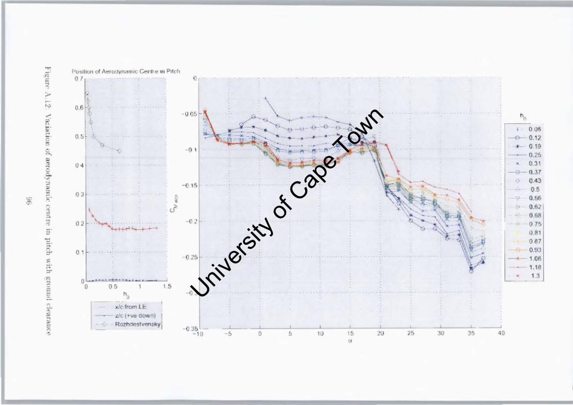
-• , -,-" -F.
" g' ~ • • , , -, >
~ i'i' ~ -, ,
" • , " -, , " , • , --,-• > , ,
1' ......... , 01 ""'<nv""""" ~ ... .. PIt"h 0' (I ,
t Mj
00
"' ", "'rlmrn LI:
--.dc(+ .... a""'~) I RO ..... ".,.h'''' ...... yl
i if
"
'" ~ ~-~~-~ -~,; -~\"Q ij;t.~ ~ ~ . ' ..
-0 . f>
"
'"
(I J50 --,"
~ I!t- • "I ""
~ I ,
\
-"------;,----;---",---,,----,-,,-----,0--~ 0 ~ 10 I ~ 2IJ 15 " ..
, ",. _ 0, 12
• (I 19 -O.2!>
, 0.31 a-- O.Jl
." " 0.$
0.62 1 Oy
'" U.S • .. , (I \!~
_ -1 _ 1 O~
I.M
" Univers
ity of
Cap
e Tow
n

. j
. ' '.~ i
,
, \
~ , L , • 0 , , -~', ... ,
l i!\ UfC.\ JJ, C" t'_, C f . I Dr ("01
!.Ii'
•
-
" ,
, o
o
" o
• ?
, - -c-- " tl37 , , , ,
l~t8llt y I -"'.W'>. "j "
Univers
ity of
Cap
e Tow
n

" , , , , ,
"
•
t¥"' ''''' ' .'
"
"
, , ;: I - ,
,----,','-----, , -,
'" , 0 r,IQ
,~
• S()"()-
,
'" "
lO-
,
• 0
'" ,7
--
Univers
ity of
Cap
e Tow
n

)
• o <
• o
./
,
f ,
>
Y"W\t tOU "f ,wr. >d\ "~l!.it , .••• , . •. H r~ III
!I!J
< , ' -<-,
;;::--"
" .
•
•
• o
1· o Univers
ity of
Cap
e Tow
n

" " " • £~ -......
" v
"' -+ a
" " " " n
" " " , , , t () , ~ ,. ,.
" "
• .. ,
" ". " " ,
'" , ~-6Q- = )( = llJ
'" , , 0 = X = w
\o-----",~. ~~~------.~ '~
/ ,
".
".
" l -" C , . ~
" " - -e
• , lOO- ~
-~ , - ~
90'0-
~
"" Univers
ity of
Cap
e Tow
n
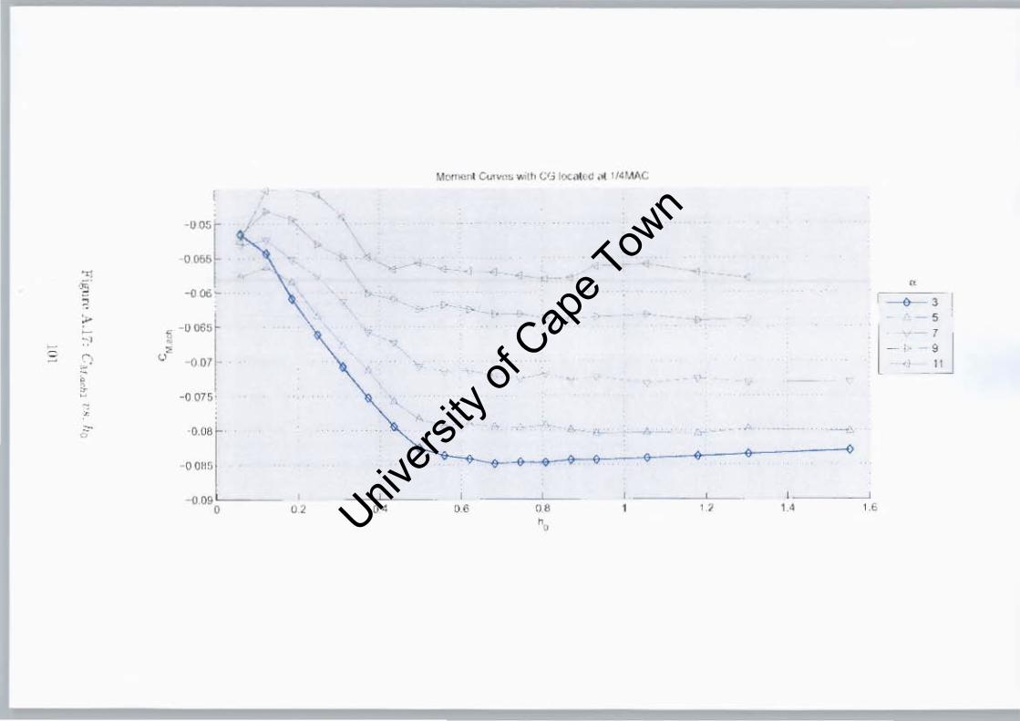
Mome'" C"",,,,, ... ,lh Vj locat\.<1 ,( 1I~1.II\C
~
-'~ f ,
"" ~ • • ~ ' " -006 - " , , ,
" C- • ,. ~
-,ool • , •• ! l U ~ ,.' ~ ~ -0 07
" " ~ " -0075' -• ~ '" " - , "
.-
• , , -0 O~5
, • • • , • -. '" , " " "" "" " " " '. Univ
ersity
of C
ape T
own

, "'l " >
"
' " -<>
I , 0 -,
c: . ., --<'y -,
> " . - -5
~ U -, , " <
., "
~-,
O.l!> " ~ " • >- -<' , -~ "L ,
~
0 o l5 -g. .. , .... j , ' , ._, ..... .L..
~ , " '" "' " " " '" •• ,~ , \, " ., ",
" ,
\ " , II 43 , " , ,
" " '" ~ 025< 1\0< 0.5 /
" " \1 A 1 \:
/ " " ,
" <::> " , " , -~ ~
U ,,,. _b " ,--~ n
"" --:>- " '" ~
,1- 31
"" , , U4t 049 " 0.51 ,~ ' " , ~ '" ". 0.57
C,
Univers
ity of
Cap
e Tow
n

Appendix B
The DHMTU Airfoil
The DHMTlJ airfoil was developed by the Department of Hydromechanics of the
Marine Technical University in St. Petersburg. They were developed specifically
for use in ground effect. The airfoils are generally characterised by a fiat section
on the lower surface of the wing, and an S-shaped mean line. The airfoils are not
defined by a mean line and a thickness distribution, as with the NACA profile, but
by separate definitions for the upper and lower surface. The DHMTlJ sections have
eight defining parameters, one for the nose radius, four for the lower surface and
three for the upper surface. The general designation of a DHMTU airfoil is given
as:
DHMTUa-b-c-d-e-f-g-h
where;
• a "--- maximum ordinate of the upper surface (%c)
• b ~ position of the maximum ordinate (%c)
• c = ordinate of the start of the fiat section (%c, below the horizontal is positive)
• d ~ position of the start of the fiat section (%c-)
• e = ordinate of the end of the fiat section (%c, below the horizontal is positive)
• f = position of the end of the fiat section (%c)
• 9 "--- slope parameter of the upper trailing edge
• h = nose radius parameter
103
Univers
ity of
Cap
e Tow
n

HI(' HI rI(,Ji ,,, .. d 01 , 1.iJ,,,,,· ,>~ P"1'lIJl~IIt.h h~d . J ~l'itll lof -1(., m 11', ~ 11 asp<'Ct ntt I(). A fI :1,
w",,.)J,,.,.·u Ih i ~<\JI\'I'" d:" rdl.· 'I!:\ h " r , ~ IS"mm, A {)UM}'F HI If) 'l 10
1-1;11 1! ,-. "'In!: 1m .hl.· "",i,, Illl " t wn I.," ..I" ",,'Il br I 10,'_'" "~ l>I' rim\' ''I ~ "",I i~ ~1,,)w1J
'" h<l"rl' 1\ 1 11.1' "" 11): ,,-;~, . .. I"u"'1\ ,jl'"",-I,·o' "ith a jotlr " ,ax JJl "JJllIIIJ("k",~ a,
ufA d"Jn\ 1'11\' " 111)\ 11* 1 Ii H~l "" , ,i,,:, "" 11"·]"",-,,. _~ ilrlj,n' fn-, ,,, 1(1';1. I." till7. chord
aud .L Wh<' r ... lhh I ... ram,·~r (Of:'
1
1 ,
'I , I
" "
1 Jb" I . -i-'ll!>
t , "1 . , ,
, • ••
Fl!~\l re e, 1. De,;gll Dr)lw i]j~, (.f J)Ff MTI 10 - 40 - ~ - HI - 1 - {ill - 11 - fl
loW
Univers
ity of
Cap
e Tow
n

Appendix C
Design Drawings
105
Univers
ity of
Cap
e Tow
n

" n , " -; ~ ~ -
" " , ;;; " , , , a ,
Univers
ity of
Cap
e Tow
n
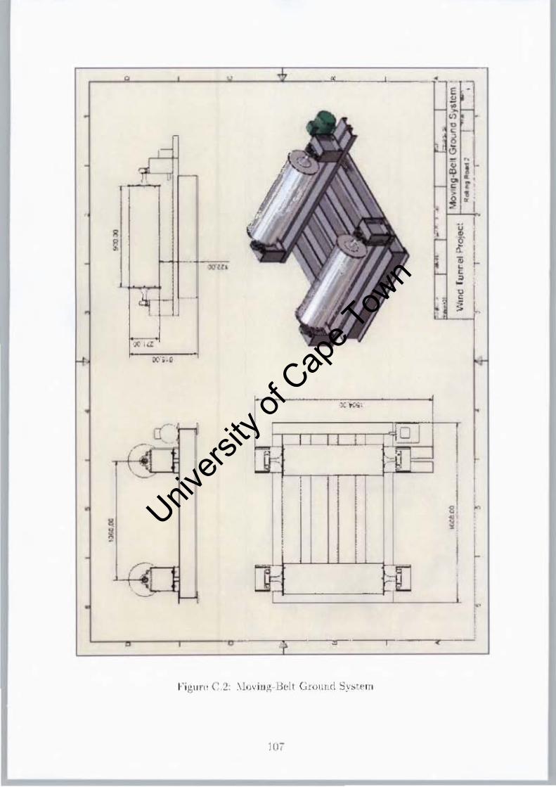
•
. -J
f-, ,
• I -
lUll<
~
""
·x ..-..... ,
ill L - I~ :-bd
,I I
, I I a I
I
• !
-•
lU,
Univers
ity of
Cap
e Tow
n

I ~··"· ........ --------------.
I • r • ,,~
I , • "".-.:'
~~ GO ,no .
"
Fig llrr c.:! Wi'l;:; Support Sy,tP[[l
Univers
ity of
Cap
e Tow
n

-
W£·
Univers
ity of
Cap
e Tow
n

Appendix D
Matlab Code
Included on CD
110
Univers
ity of
Cap
e Tow
n

Appendix E
Data
Included on CD
111
Univers
ity of
Cap
e Tow
n


![SMV [McMillan 93]](https://img.pdfslide.us/doc/110x75/5681572a550346895dc4c47a/smv-mcmillan-93.jpg)