"Aerodynamic Computations on Unstructured Grids Using a Newton-Krylov Approach," AIAA

Three-Dimensional Aerodynamic Computations on

Unstructured Grids Using a Newton-Krylov Approach

P. Wong∗, and D. W. Zingg†

University of Toronto Institute for Aerospace Studies

4925 Dufferin Street, Toronto, Ontario

Canada, M3H 5T6

A Newton-Krylov algorithm is presented for the compressible Navier-Stokes equationsin three dimensions on unstructured grids. The algorithm uses a preconditioned matrix-freeKrylov method to solve the linear system that arises in the Newton iterations. Incompletefactorization is used as the preconditioner, based on an approximate Jacobian matrix afterthe reverse Cuthill-McKee reordering of the unknowns. Approximate viscous operatorsthat involve only the nearest neighboring terms are studied to construct an efficient andeffective preconditioner. Two incomplete factorization techniques are examined: one basedon a level-of-fill approach while the other utilizes a threshold strategy. The performanceof the algorithm is demonstrated with numerical studies over the ONERA M6 wing andthe DLR-F6 wing-body configuration. A ten-order-of-magnitude residual reduction can beobtained in 20-25 hours on a single processor for a mesh with roughly 500,000 nodes.

I. Introduction

After many years of development, computational fluid dynamics has become an important aerodynamicdesign tool.1,2 The current technology is capable of analyzing viscous compressible flows over completeaircraft configurations. Two AIAA Drag Prediction Workshops were organized to assess the capability ofcurrent solvers when applied to such flows. Lee-Rausch et al.3 summarized the results of three state-of-the-art unstructured grid solvers when applied to solve the the DLR-F6 transport configuration in the secondDrag Prediction Workshop. May et al.4 summarized the results for the same configuration from two well-known structured grid solvers. Other studies include the work of Luo et al.,5 and Brodersen and Sturmer.6

With parallelization, flow solutions can be obtained in several hours using a grid with three million nodes.However, the grid density is insufficient to achieve grid convergence. Moreover, variations are observedbetween solutions from different codes. In order to improve the accuracy of the technology, finer grids, meshadaptation and higher-order methods have been suggested. Research also continues in the development offaster algorithms to reduce computational time.

The Newton-Krylov method is an efficient method to solve the Navier-Stokes equations.7 Its implicitnature has good potential in turbulent applications when stretched meshes are used to calculate the viscousboundary layers. Some early work for aerodynamic applications can be found in the studies by Venkatakrish-nan and Mavriplis,8 Barth and Linton,9 Nielsen et al.,10 and Anderson et al.11 Blanco and Zingg12 performeda study comparing quasi-Newton, standard Newton, and matrix-free Newton methods. They developed afast solver on triangular grids using a matrix-free inexact-Newton approach together with an approximate-Newton startup strategy. Pueyo and Zingg13 developed a preconditioned matrix-free Newton-Krylov algo-rithm. Their optimized algorithm is found to converge faster and more reliably than an approximate Newtonalgorithm and an approximately-factored multigrid algorithm. Geuzaine et al.14,15 studied mesh sequenc-ing as well as multigrid preconditioning with the Newton-Krylov method. Nemec and Zingg16 applied aNewton-Krylov method to numerical optimization. The same approach is applied to solve the flow equations

∗Ph.D. Candidate, [email protected]†Professor, Senior Member AIAA, Tier I Canada Research Chair in Computational Aerodynamics, 2004 Guggenheim Fellow,

http://goldfinger.utias.utoronto.ca/dwz

1 of 15

American Institute of Aeronautics and Astronautics

as well as the adjoint equations to calculate the objective function gradients. Chisholm and Zingg17,18 de-veloped a strategy which provides effective and efficient startup for turbulent flows with the Newton-Krylovalgorithm. Manzano et al.19 applied the Newton-Krylov algorithm to three-dimensional inviscid flows usingunstructured grids.

The purpose of this work is to extend the algorithm of Manzano et al. to turbulent flows on hybrid un-structured grids. The goal is to develop an efficient and robust algorithm for three-dimensional aerodynamicflows. Different aspects of the algorithm are studied and discussed in the paper, including preconditioningand startup strategy. The performance of the algorithm is demonstrated over a wing as well as a wing-bodyconfiguration.

II. Governing Equations

The governing equations are the compressible Navier-Stokes equations. These equations describe theconservation of mass, momentum and total energy for a viscous compressible flow. For an arbitrary controlvolume Ω, the integral from of the equations can be written as:

∂

∂t

∫

Ω

QdV +∫

∂Ω

F · ndS =∫

∂Ω

G · ndS (1)

where Q is the set of conservative flow variables (density ρ, momentum components ρu, ρv, ρw, and totalenergy ρE), F is the inviscid flux tensor, and G is the flux tensor associated with viscosity and heatconduction. These quantities can be written as:

Q =

ρ

ρu

ρv

ρw

ρE

, F =

ρu

ρu2 + p

ρuv

ρuw

u(ρE + p)

i +

ρv

ρuv

ρv2 + p

ρvw

v(ρE + p)

j +

ρw

ρuw

ρvw

ρw2 + p

w(ρE + p)

k (2)

G =

0τxx

τxy

τxz

uτxx + vτxy + wτxz − qx

i+

0τyx

τyy

τyz

uτyx + vτyy + wτyz − qy

j+

0τzx

τzy

τzz

uτzx + vτzy + wτzz − qz

k (3)

For a Newtonian fluid in local thermodynamic equilibrium, Stokes relation is valid. The viscous stress tensorτ can be related to the dynamic viscosity µ and the strain rate tensor using:

τ = µ

2ux uy + vx uz + wx

vx + uy 2vy vz + wy

wx + uz wy + vz 2wz

− 2

3µ (ux + vy + wz) I (4)

where I is the unit tensor, and ux denotes ∂u/∂x and so forth. The heat flux vector is given by Fourier’slaw q = −k∇T . The thermal conductivity is related to the dynamic viscosity through the Prandtl numberPr = cpµ/k. Sutherland’s law is used to calculate the dynamic viscosity. Assuming the fluid behaves as aperfect gas, the pressure p can be written in terms of the conservative variables to close the system:

p = (γ − 1)[ρE − 1

2ρ

(u2 + v2 + w2

)](5)

III. Turbulence Modeling

We solve the Reynolds-averaged Navier-Stokes equations for turbulent flows. The Reynolds-stress tensoris modeled using the Boussinesq approximation and introducing an eddy-viscosity term. The turbulent eddyviscosity is modeled with the one-equation Spalart and Allmaras turbulence model.20 In differential form the

2 of 15


model is written as:

∂ν

∂t+ (v · ∇) ν = cb1(1− ft2)Sν +

1σ

[∇ · ((ν + ν)∇ν) + cb2(∇ν)2]

−[cw1fw − cb1

κ2ft2

] (ν

d

)2

+ ft1∆U2 (6)

where v is the velocity vector, and ∆U is the norm of the velocity difference between a field point and thetrip point. The model is solved in a form fully-coupled with the mean-flow equations. The eddy viscosityνt is calculated from the working variable ν, and ν denotes the kinematic viscosity. The terms on the right-hand side of the equation are the production term, the diffusion term, the destruction term, and the tripterm respectively. Production of eddy viscosity is proportional to a vorticity-like term S, which containsthe magnitude of the vorticity in the mean flow. The destruction term governs the dissipation of the eddyviscosity due to blocking effects of the wall. The distance to the closest wall is denoted as d, κ is the vonKarman constant, and fw is a function that models near-wall effects. The model includes a trip term thatmodels laminar-to-turbulent flow transition. Transition locations are not predicted and are specified by theuser. Alternatively, the flow can be assumed to be fully turbulent by setting the trip functions ft1 and ft2

to zero. This assumes transition occurs at the leading edge. Closure coefficients cb1, σ, cb2, and cw1 are thesame as those given by Spalart and Allmaras.21 The wall boundary condition is ν = 0. A value of ν∞/10 isused as the free-stream condition for ν, where ν∞ is the kinematic viscosity in the free stream.

Ashford22 proposed a modification to S in the production term. The modification is found to producebetter numerical properties17 and is adopted in the current work.

IV. Spatial Discretization

The spatial discretization follows that used by Mavriplis and Venkatakrishnan23 for hybrid unstructuredgrids. A cell-vertex approach is utilized with centroidal-median-dual control volumes constructed aroundsource-grid vertices. A finite-volume discretization is obtained by integrating the fluxes over the boundaryof the control volume. The value of the flux at each control volume face is computed by averaging the fluxesin the two control volumes on either side of the face:

fik ' 12

[F(Qi) + F(Qk)] · ~nik + Dik (7)

where fik is the inviscid numerical flux on the face ik with neighboring cells i and k, ~nik is the area-weightednormal of the face ik, and Dik is the dissipation operator.

Numerical dissipation is added for stability and resolving shocks. A matrix dissipation scheme is used.It is constructed from the undivided Laplacian and biharmonic operators:

Dik = −12|Aik|

[ε(2)ik (Qk −Qi)− ε

(4)ik (Lk − Li)

]

Li =∑

k

(Qk −Qi)

where

ε(2)i =

∑

k

κ2|pk − pi|pk + pi

andε(4)i = max

(0, κ4 − ε

(2)i

)(8)

where εik is calculated by averaging the values from the two neighboring cells i and k. Two parameters κ2

and κ4 control the addition of second- and fourth-difference dissipation. A pressure switch selects the second-difference operator in the presence of shocks, while the fourth-difference operator is used in areas of smoothflow. The Laplacian operator is denoted as L, and |A| is the absolute value of the inviscid flux Jacobian.Small eigenvalues in the Jacobian may occur near stagnation points and sonic points using this approach.This affects convergence and can be avoided by introducing two parameters Vl and Vn, as described bySwanson and Turkel.24 Values of κ2 = 2, κ4 = 0.1, Vl = Vn = 0.25 are used in the current work. A centered

3 of 15


scheme is utilized for the diffusive-flux term. The convective terms in the turbulence model are discretizedusing a first-order scheme, as suggested by Spalart and Allmaras.20

Boundary conditions are enforced by extrapolating the solution to boundary faces and imposing the ap-propiate boundary conditions. They are handled in a fully-implicit manner in order to obtain fast convergenceusing Newton’s method.

V. Newton-Krylov Algorithm

A. Newton iterations

After spatial discretization the steady-state governing equations become a system of nonlinear algebraicequations R(Q) = 0. We use Newton’s method, which has the potential for fast convergence, to obtain asolution of these equations. At each Newton iteration, we need to solve a linear system for the solutionupdate: (

∂R∂Q

)n

∆Qn = −R(Qn) (9)

Qn+1 = Qn + ∆Qn (10)

This procedure is repeated until the solution satisfies some convergence tolerance.Newton’s method may not converge when the solution is far from the final result because (9) is a rea-

sonable approximation to R(Qn+1) = 0 only for small ∆Qn. One alternative to improve robustness of themethod is to include a time step and apply an implicit-Euler approach. The matrix of the linear systembecomes:

A(Qn) =Ω

∆tn+

(∂R∂Q

)n

(11)

where Ω/∆tn represents a diagonal matrix of cell volumes divided by local time steps. When the time stepsare increased towards infinity, Newton’s method is approached. This provides some flexibility to controlrobustness versus efficiency during the solution process.

B. The linear system

The linear system that arises in the Newton iterations is large and sparse for practical problems. In addition,the matrix is non-symmetric due to the hyperbolic nature of the Navier-Stokes equations. Krylov subspacemethods can be used to solve this class of problems. In particular, the generalized minimum residual method(GMRES) developed by Saad and Schultz25 is found to be effective for aerodynamic applications. Thismethod has the property of minimizing the 2-norm of the residual over all vectors in the Krylov subspace. Anew search direction is constructed every iteration and is added to the subspace, thus progressively improvingthe solution. On the other hand, more search directions incur extra memory and computational costs. Forlarge problems, this limits the maximum number of iterations that can be used. The restarted version ofthe algorithm is one alternative to reduce memory usage. However, the solution may stagnate for indefinitematrices. A more effective way to reduce the number of iterations is to use preconditioning.

Since (9) is only an approximation to zero the residual at the next iteration, complete solving of thesystem is found to be unnecessary to obtain quadratic convergence.26 An inexact Newton method can beutilized which leads to efficient algorithms by avoiding oversolving of the linear system. The linear systemis solved until the solution satisfies a tolerance specified by a parameter ηn:

||R(Qn) +A(Qn)∆Qn|| ≤ ηn||R(Qn)|| (12)

The choice of this parameter is a compromise between the accuracy of the update and efficiency. Choosingηn too small will result in over-solving of the linear system, which slows down the algorithm.

The GMRES algorithm allows a matrix-free implementation; the matrix of the linear system is notrequired explicitly. The matrix-vector product can be calculated using finite differences:

Av ' R(Q+ εv)−R(Q)ε

+Ω∆t

v (13)

4 of 15


This allows quadratic convergence of Newton’s method because the matrix of the linear system is a com-plete linearization of the residual vector. Moreover, this approach reduces memory usage and avoids somedifficulties during linearization. We use a matrix-free stepsize of:

ε||v|| =√

10−10 (14)

following recent results from Chisholm and Zingg.18

C. Preconditioning

Preconditioning transforms the linear system (written as Ax = b) to one which has the same solution, butis easier to solve by an iterative solver. This reduces the number of inner iterations required to solve thesystem. The right-preconditioned GMRES algorithm is based on solving

AM−1u = b, u = Mx (15)

where M is the preconditioner. The matrix AM−1 should have a better condition number than the originalmatrix A. In practice, an iterative solver will perform efficiently if the eigenvalues of AM−1 are clusteredaround unity. An effective preconditioner M is chosen so that M−1 approximates A−1, while M−1 is easyto compute. This operation is performed every outer iteration.

Pueyo and Zingg13 have constructed a preconditioner which works well for many aerodynamic flows. Itis based on an incomplete-lower-upper factorization (ILU(p)) of an approximate Jacobian after the reverseCuthill-McKee reordering of the unknowns. The parameter p controls the amount of fill. Increasing its valueresults in more accurate factors with extra storage and computational costs. The approximate Jacobian isconstructed by a linearization of the flow equations with only nearest-neighbor contributions. This improvesthe diagonal dominance of the matrix, and was found by Pueyo and Zingg to be more effective than thecomplete Jacobian. The coefficient of the dissipation term is calculated using

ε(2)p = ε(2) + σε(4) (16)

with a parameter σ, where ε(2) and ε(4) are the coefficients of the dissipation term as defined in (8). Thesubscript p denotes the preconditioner. Chisholm and Zingg17 have extended the approximate Jacobian toincorporate the matrix-dissipation scheme. They suggest two parameters Vl,p and Vn,p to avoid overly smalldiagonal elements in the matrix. Hence the blend of scalar and matrix dissipation can be altered in theapproximate Jacobian used to form the preconditioner. Values typically used are Vl,p = Vn,p = 0.6.

Besides the aforementioned preconditioner based on a level-of-fill strategy, factorization with a thresholdstrategy (ILUT) is also considered in this work. Pueyo and Zingg compared the two preconditioners andfound that the level-of-fill approach is more efficient for two-dimensional flow computations. The thresholdstrategy is reconsidered in this work since it provides more control over the number of nonzero entries inthe preconditioner, which is important in three dimensions. The threshold strategy ILUT(l,τ) is based ondropping elements in the factorization according to their magnitude rather than their locations. The droptolerance τ determines the elements to be neglected, while l controls how many elements are kept.

D. Preconditioning of the viscous term

The baseline viscous term is calculated by:(∫

∂Ω

G · ndS

)

i

'∑

k

Gik · ~nik (17)

where Gik = G(Qik,∇Qik) is the viscous flux on a face ik, with neighboring cells i and k. ∇Q is the gradientof the flow variables. This is calculated using:

∇Qik =12

(∇Qi +∇Qk) (18)

where∇Qi ' 1

Ωi

∑

k

Qik~nik (19)

5 of 15


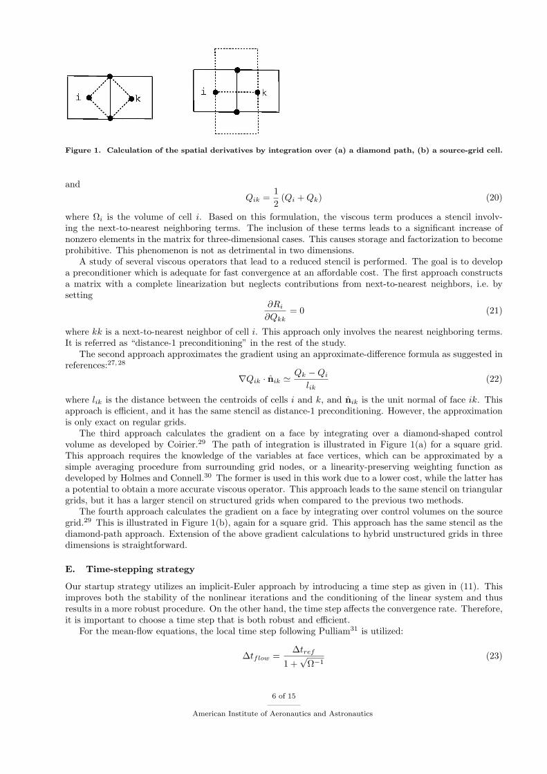
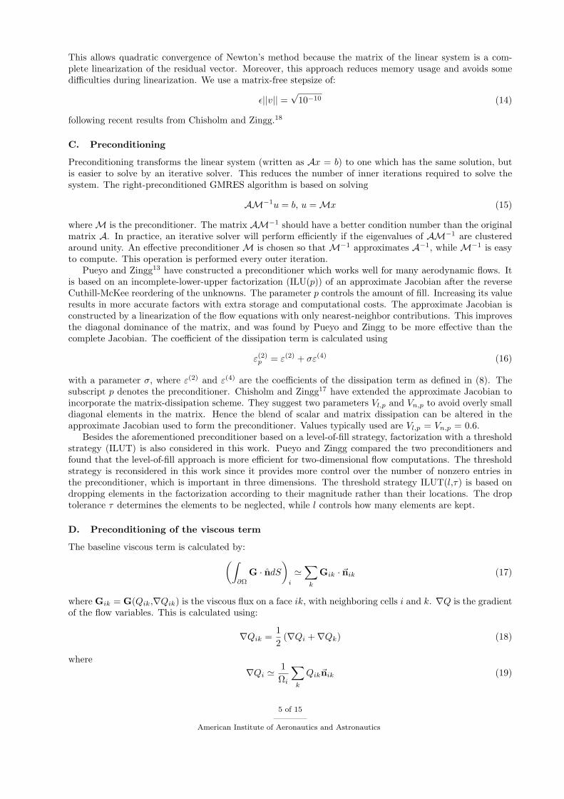
Figure 1. Calculation of the spatial derivatives by integration over (a) a diamond path, (b) a source-grid cell.

andQik =

12

(Qi + Qk) (20)

where Ωi is the volume of cell i. Based on this formulation, the viscous term produces a stencil involv-ing the next-to-nearest neighboring terms. The inclusion of these terms leads to a significant increase ofnonzero elements in the matrix for three-dimensional cases. This causes storage and factorization to becomeprohibitive. This phenomenon is not as detrimental in two dimensions.

A study of several viscous operators that lead to a reduced stencil is performed. The goal is to developa preconditioner which is adequate for fast convergence at an affordable cost. The first approach constructsa matrix with a complete linearization but neglects contributions from next-to-nearest neighbors, i.e. bysetting

∂Ri

∂Qkk= 0 (21)

where kk is a next-to-nearest neighbor of cell i. This approach only involves the nearest neighboring terms.It is referred as “distance-1 preconditioning” in the rest of the study.

The second approach approximates the gradient using an approximate-difference formula as suggested inreferences:27,28

∇Qik · nik ' Qk −Qi

lik(22)

where lik is the distance between the centroids of cells i and k, and nik is the unit normal of face ik. Thisapproach is efficient, and it has the same stencil as distance-1 preconditioning. However, the approximationis only exact on regular grids.

The third approach calculates the gradient on a face by integrating over a diamond-shaped controlvolume as developed by Coirier.29 The path of integration is illustrated in Figure 1(a) for a square grid.This approach requires the knowledge of the variables at face vertices, which can be approximated by asimple averaging procedure from surrounding grid nodes, or a linearity-preserving weighting function asdeveloped by Holmes and Connell.30 The former is used in this work due to a lower cost, while the latter hasa potential to obtain a more accurate viscous operator. This approach leads to the same stencil on triangulargrids, but it has a larger stencil on structured grids when compared to the previous two methods.

The fourth approach calculates the gradient on a face by integrating over control volumes on the sourcegrid.29 This is illustrated in Figure 1(b), again for a square grid. This approach has the same stencil as thediamond-path approach. Extension of the above gradient calculations to hybrid unstructured grids in threedimensions is straightforward.

E. Time-stepping strategy

Our startup strategy utilizes an implicit-Euler approach by introducing a time step as given in (11). Thisimproves both the stability of the nonlinear iterations and the conditioning of the linear system and thusresults in a more robust procedure. On the other hand, the time step affects the convergence rate. Therefore,it is important to choose a time step that is both robust and efficient.

For the mean-flow equations, the local time step following Pulliam31 is utilized:

∆tflow =∆tref

1 +√

Ω−1(23)

6 of 15


Case M∞ α Re Geometry Grid size

1 0.8395 3.06 11.7 × 106 ONERA M6 179,0002 0.8395 3.06 11.7 × 106 ONERA M6 480,0003 0.5 0.0 3.0 × 106 DLR-F6 431,000

Table 1. Flow conditions, geometry and grid size.

where Ω is the local cell volume. One way to calculate the reference time step ∆tref is to follow the switchedevolution relaxation approach from Mulder and van Leer:32

∆tref = α||R||−β2 (24)

where ||R||2 is the residual norm, and α and β are parameters. The idea is to increase the time step ininverse proportion to the residual norm, thus approaching Newton’s method as the residual converges tozero. Other choices include the use of a constant value or a geometric series. These seem to be better choicesfor the startup stages due to their flexibility.

The turbulence model requires small time steps during the startup stage. Otherwise, unphysical negativevalues of ν will occur and cause the solution to become unstable. However, the use of small time stepsslows down the convergence rate. Spalart and Allmaras20 suggested the use of an M-type Jacobian matrixto prevent ν to become negative at a penalty on the convergence rate. Chisholm and Zingg17 provide analternative approach using a spatially varying time step during the start-up phase. This approach attemptsto prevent negative ν by locally reducing the time step. It allows larger time steps to be used elsewhere inthe domain. Moreover, a matrix-free approach can be utilized due to the lack of modification in the Jacobianmatrix. This provides an effective startup strategy.

Chisholm and Zingg’s time step can be summarized as follows:

∆tturb =

∆tflow if |δe| < δm

|∆tlimit| otherwise(25)

where δe is an estimate of the solution update, and δm = rν is the maximum allowable change specified bya parameter r. A typical value of r is 0.3. When the estimate exceeds the allowable value, the time step isreduced to ∆tlimit. Otherwise, the mean-flow time step is utilized. The estimate is determined by applyingNewton’s method to the local uncoupled turbulence equation:

JDδe = −R (26)

where JD is the Jacobian entry on the diagonal in the turbulence model equation, and R is the right-handside of the turbulence equation. The limiting time step is determined such that it reduces the estimate tothe allowable value, i.e. |δe| = δm. This can be calculated solving the following equation for ∆tlimit:

(Ω

∆tlimit+ JD

)δm = −R (27)

Further details about the local time step can be found in the original work by Chisholm and Zingg.18

VI. Results

Three turbulent cases are studied. The first two are transonic flows over a wing. The third case is asubsonic flow over a wing-body configuration. Flow conditions are summarized in Table 1. The cases areassumed to be fully turbulent. All cases are run on a single 1 GHz alpha EV68 processor at the high-performance advanced computing facility in the University of Toronto Institute for Aerospace Studies.

A. Grid generation

The ICEMCFD grid generator is utilized to generate the grids for the test cases. Prism layers are generatedby extruding 15 layers of prism elements from the surface mesh using a growth ratio of 1.5. The off-wall

7 of 15


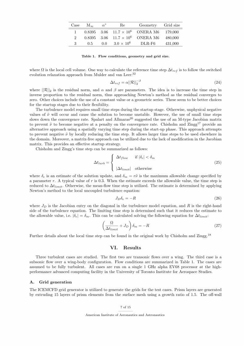
Figure 2. ONERA M6 wing grid with 179,000 nodes. Figure 3. ONERA M6 wing grid with 480,000 nodes.

Figure 4. DLR-F6 wing-body grid with 431,000nodes.

Figure 5. Close-up view at the wing-body junction.

spacing is 10−6 times the chord at the wing root. The far-field boundary is specified at 12 wing-root chordsfrom the wing. It is located at 12 times the length of the fuselage from the wing-body configuration.

The geometry and grid size are summarized in Table 1. Figure 2 shows the grid for Case 1, with aclose-up of the leading edge at the wing root. The grid has 179,000 nodes consisting of both tetrahedral andprismatic cells. Figure 3 shows the grid for Case 2. It is a finer grid with 480,000 nodes. The wing surface aswell as the volume region above the wing are refined to provide better resolution of the shock wave. Figure 4shows the grid with 431,000 nodes for Case 3. A close-up of the wing-body junction is shown in Figure 5.None of these grids is expected to be sufficiently fine to achieve a low numerical error in drag.

B. Solver parameters

The linear system is solved using a matrix-free non-restarted version of GMRES with 50 Krylov vectors. Alinear system tolerance of η = 10−2 is used in this work, based on a study given in a later part of the paper.The preconditioner is ILU(1) based on an approximate Jacobian matrix after the reverse Cuthill-McKeereordering of the unknowns. Values of σ = 10, Vl,p = Vn,p = 0.6 are utilized in the approximate Jacobian.

Startup is initiated using a first-order scalar scheme before switching to the matrix-dissipation scheme.Switching is triggered when the mean-flow residual converges to 10−4. The first-order scheme is defined withε(2) = 1/4, ε(4) = 0, and Vl = Vn = 1, where ε(2) and ε(4) are the coefficients of the dissipation term as givenin (8).

One set of time step parameters is used for the three cases in this work. We use ∆tref = 1 for the firstthree iterations. After that, ∆tref is set to 20 and the value is doubled every 5 iterations. To prevent thesolution from becoming unstable with too large a time step, the solution update is checked every Newtoniteration. If nonphysical flow quantities are encountered, (i.e. negative pressure or density), then the recentsolution update is rejected and ∆tref for the next iteration is halved. A similar safeguarding mechanism is

8 of 15


1e-12

1e-10

1e-08

1e-06

0.0001

0.01

1

100

0 1 2 3 4 5 6 7 8

0 1000 2000 3000 4000 5000

Res

idua

l

CPU time (hours)

RHS evaluations

Dist-1Approx-Diff

Diamond-PathSource-Grid

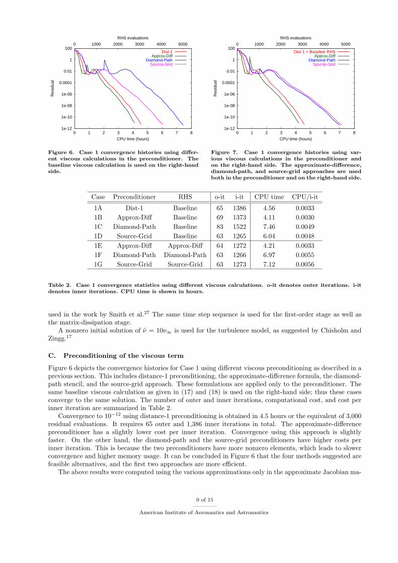
Figure 6. Case 1 convergence histories using differ-ent viscous calculations in the preconditioner. Thebaseline viscous calculation is used on the right-handside.

1e-12

1e-10

1e-08

1e-06

0.0001

0.01

1

100

0 1 2 3 4 5 6 7 8

0 1000 2000 3000 4000 5000

Res

idua

l

CPU time (hours)

RHS evaluations

Dist-1 + Baseline RHSApprox-Diff

Diamond-PathSource-Grid

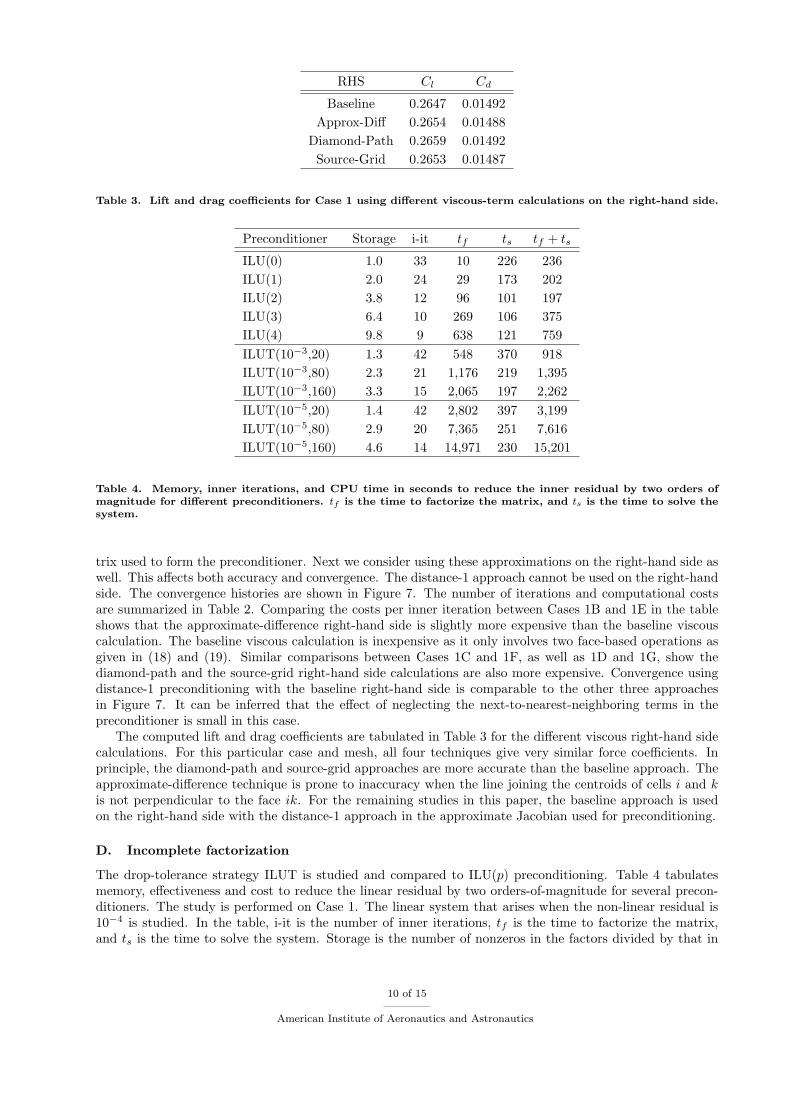
Figure 7. Case 1 convergence histories using var-ious viscous calculations in the preconditioner andon the right-hand side. The approximate-difference,diamond-path, and source-grid approaches are usedboth in the preconditioner and on the right-hand side.

Case Preconditioner RHS o-it i-it CPU time CPU/i-it

1A Dist-1 Baseline 65 1386 4.56 0.00331B Approx-Diff Baseline 69 1373 4.11 0.00301C Diamond-Path Baseline 83 1522 7.46 0.00491D Source-Grid Baseline 63 1265 6.04 0.00481E Approx-Diff Approx-Diff 64 1272 4.21 0.00331F Diamond-Path Diamond-Path 63 1266 6.97 0.00551G Source-Grid Source-Grid 63 1273 7.12 0.0056

Table 2. Case 1 convergence statistics using different viscous calculations. o-it denotes outer iterations. i-itdenotes inner iterations. CPU time is shown in hours.

used in the work by Smith et al.27 The same time step sequence is used for the first-order stage as well asthe matrix-dissipation stage.

A nonzero initial solution of ν = 10ν∞ is used for the turbulence model, as suggested by Chisholm andZingg.17

C. Preconditioning of the viscous term

Figure 6 depicts the convergence histories for Case 1 using different viscous preconditioning as described in aprevious section. This includes distance-1 preconditioning, the approximate-difference formula, the diamond-path stencil, and the source-grid approach. These formulations are applied only to the preconditioner. Thesame baseline viscous calculation as given in (17) and (18) is used on the right-hand side; thus these casesconverge to the same solution. The number of outer and inner iterations, computational cost, and cost perinner iteration are summarized in Table 2.

Convergence to 10−12 using distance-1 preconditioning is obtained in 4.5 hours or the equivalent of 3,000residual evaluations. It requires 65 outer and 1,386 inner iterations in total. The approximate-differencepreconditioner has a slightly lower cost per inner iteration. Convergence using this approach is slightlyfaster. On the other hand, the diamond-path and the source-grid preconditioners have higher costs perinner iteration. This is because the two preconditioners have more nonzero elements, which leads to slowerconvergence and higher memory usage. It can be concluded in Figure 6 that the four methods suggested arefeasible alternatives, and the first two approaches are more efficient.

The above results were computed using the various approximations only in the approximate Jacobian ma-

9 of 15


RHS Cl Cd

Baseline 0.2647 0.01492Approx-Diff 0.2654 0.01488

Diamond-Path 0.2659 0.01492Source-Grid 0.2653 0.01487

Table 3. Lift and drag coefficients for Case 1 using different viscous-term calculations on the right-hand side.

Preconditioner Storage i-it tf ts tf + ts

ILU(0) 1.0 33 10 226 236ILU(1) 2.0 24 29 173 202ILU(2) 3.8 12 96 101 197ILU(3) 6.4 10 269 106 375ILU(4) 9.8 9 638 121 759ILUT(10−3,20) 1.3 42 548 370 918ILUT(10−3,80) 2.3 21 1,176 219 1,395ILUT(10−3,160) 3.3 15 2,065 197 2,262ILUT(10−5,20) 1.4 42 2,802 397 3,199ILUT(10−5,80) 2.9 20 7,365 251 7,616ILUT(10−5,160) 4.6 14 14,971 230 15,201

Table 4. Memory, inner iterations, and CPU time in seconds to reduce the inner residual by two orders ofmagnitude for different preconditioners. tf is the time to factorize the matrix, and ts is the time to solve thesystem.

trix used to form the preconditioner. Next we consider using these approximations on the right-hand side aswell. This affects both accuracy and convergence. The distance-1 approach cannot be used on the right-handside. The convergence histories are shown in Figure 7. The number of iterations and computational costsare summarized in Table 2. Comparing the costs per inner iteration between Cases 1B and 1E in the tableshows that the approximate-difference right-hand side is slightly more expensive than the baseline viscouscalculation. The baseline viscous calculation is inexpensive as it only involves two face-based operations asgiven in (18) and (19). Similar comparisons between Cases 1C and 1F, as well as 1D and 1G, show thediamond-path and the source-grid right-hand side calculations are also more expensive. Convergence usingdistance-1 preconditioning with the baseline right-hand side is comparable to the other three approachesin Figure 7. It can be inferred that the effect of neglecting the next-to-nearest-neighboring terms in thepreconditioner is small in this case.

The computed lift and drag coefficients are tabulated in Table 3 for the different viscous right-hand sidecalculations. For this particular case and mesh, all four techniques give very similar force coefficients. Inprinciple, the diamond-path and source-grid approaches are more accurate than the baseline approach. Theapproximate-difference technique is prone to inaccuracy when the line joining the centroids of cells i and kis not perpendicular to the face ik. For the remaining studies in this paper, the baseline approach is usedon the right-hand side with the distance-1 approach in the approximate Jacobian used for preconditioning.

D. Incomplete factorization

The drop-tolerance strategy ILUT is studied and compared to ILU(p) preconditioning. Table 4 tabulatesmemory, effectiveness and cost to reduce the linear residual by two orders-of-magnitude for several precon-ditioners. The study is performed on Case 1. The linear system that arises when the non-linear residual is10−4 is studied. In the table, i-it is the number of inner iterations, tf is the time to factorize the matrix,and ts is the time to solve the system. Storage is the number of nonzeros in the factors divided by that in

10 of 15


1e-12

1e-10

1e-08

1e-06

0.0001

0.01

1

100

0 5 10 15 20 25 30 35 40

0 2000 4000 6000 8000 10000

Res

idua

l

CPU time (hours)

RHS evaluations

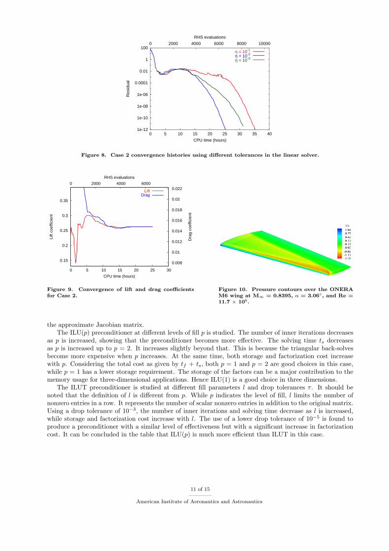
η = 10-1

η = 10-2

η = 10-3

Figure 8. Case 2 convergence histories using different tolerances in the linear solver.

0.15

0.2

0.25

0.3

0.35

0 5 10 15 20 25 30

0.008

0.01

0.012

0.014

0.016

0.018

0.02

0.022 0 2000 4000 6000

Lift

coef

ficie

nt

Dra

g co

effic

ient

CPU time (hours)

RHS evaluations

LiftDrag

Figure 9. Convergence of lift and drag coefficientsfor Case 2.

Figure 10. Pressure contours over the ONERAM6 wing at M∞ = 0.8395, α = 3.06, and Re =11.7 × 106.

the approximate Jacobian matrix.The ILU(p) preconditioner at different levels of fill p is studied. The number of inner iterations decreases

as p is increased, showing that the preconditioner becomes more effective. The solving time ts decreasesas p is increased up to p = 2. It increases slightly beyond that. This is because the triangular back-solvesbecome more expensive when p increases. At the same time, both storage and factorization cost increasewith p. Considering the total cost as given by tf + ts, both p = 1 and p = 2 are good choices in this case,while p = 1 has a lower storage requirement. The storage of the factors can be a major contribution to thememory usage for three-dimensional applications. Hence ILU(1) is a good choice in three dimensions.

The ILUT preconditioner is studied at different fill parameters l and drop tolerances τ . It should benoted that the definition of l is different from p. While p indicates the level of fill, l limits the number ofnonzero entries in a row. It represents the number of scalar nonzero entries in addition to the original matrix.Using a drop tolerance of 10−3, the number of inner iterations and solving time decrease as l is increased,while storage and factorization cost increase with l. The use of a lower drop tolerance of 10−5 is found toproduce a preconditioner with a similar level of effectiveness but with a significant increase in factorizationcost. It can be concluded in the table that ILU(p) is much more efficient than ILUT in this case.

11 of 15


Convergence criterion CPU time (hours)

0.5% of CL 17.20.1% of CL 18.80.01% of CL 20.60.5% of CD 16.90.1% of CD 18.60.01% of CD 20.5

Table 5. Convergence data for the lift and drag coefficients for Case 2.

1e-12

1e-10

1e-08

1e-06

0.0001

0.01

1

100

10000

0 5 10 15 20

0 2000 4000 6000

Res

idua

l

CPU time (hours)

RHS evaluations

First-orderMatrix Diss

Figure 11. Case 3 convergence history. Figure 12. Pressure contours over the DLR-F6wing-body configuration at M∞ = 0.5, α = 0,and Re = 3 × 106.

E. Convergence results

Figure 8 shows the convergence for Case 2 using different linear system tolerances. ILU(1) is used as thepreconditioner. Convergence to 10−12 is obtained in 25 hours or the equivalent of 6,000 residual evaluationsfor this half-million-node grid using a linear system tolerance of η = 10−2. It requires 148 outer and 2,300inner iterations. The use of a larger inner tolerance of 10−1 is found to produce a longer startup stage withan increased number of outer iterations, while a smaller inner tolerance of 10−3 leads to slower convergencewith respect to CPU time resulting from an increased number of inner iterations.

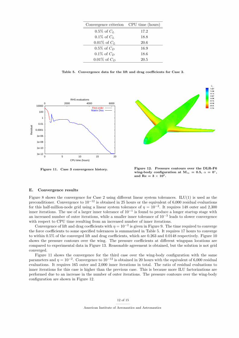
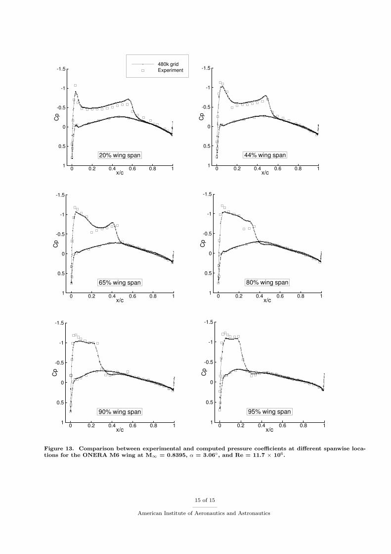
Convergence of lift and drag coefficients with η = 10−2 is given in Figure 9. The time required to convergethe force coefficients to some specified tolerances is summarized in Table 5. It requires 17 hours to convergeto within 0.5% of the converged lift and drag coefficients, which are 0.263 and 0.0148 respectively. Figure 10shows the pressure contours over the wing. The pressure coefficients at different wingspan locations arecompared to experimental data in Figure 13. Reasonable agreement is obtained, but the solution is not gridconverged.

Figure 11 shows the convergence for the third case over the wing-body configuration with the sameparameters and η = 10−2. Convergence to 10−12 is obtained in 20 hours with the equivalent of 6,000 residualevaluations. It requires 165 outer and 2,000 inner iterations in total. The ratio of residual evaluations toinner iterations for this case is higher than the previous case. This is because more ILU factorizations areperformed due to an increase in the number of outer iterations. The pressure contours over the wing-bodyconfiguration are shown in Figure 12.

12 of 15


VII. Conclusions

A Newton-Krylov algorithm is presented for turbulent aerodynamic flows on three-dimensional unstruc-tured grids. Residual convergence to 10−12 for grids with a half-million nodes can be obtained in 20-25 hourson a single processor.

The inclusion of the next-to-nearest neighboring terms in the viscous operator causes preconditioning tobecome impractical for three-dimensional applications. Four approaches are suggested as alternatives and arefound to be viable options. Distance-1 viscous preconditioning in conjunction with the baseline distance-2viscous calculation on the right-hand side is selected based on both efficiency and accuracy considerations.The ILU(p) and ILUT preconditioners are studied; the former is found to be more efficient.

Current results have motivated further research to improve the efficiency of the current algorithm. Futurework includes further investigation of startup strategies. The algorithm will also be extended to parallelcomputers to further reduce computational time. The improved algorithm will be applied to computationson finer grids to produce grid converged solutions.

VIII. Acknowledgments

This research was supported by Bombardier Aerospace and an OGS grant of the Government of Ontario.The authors would like to thank Prof. J. V. Lassaline for many useful discussions.

References

1Johnson, F. T., Tinoco, E. N., and Yu, N. J., “Thirty Years of Development and Application of CFD at Boeing CommercialAirplanes, Seattle,” AIAA Paper 2003-3439 , 2003.

2Nelson, T. E. and Zingg, D. W., “Fifty Years of Aerodynamics: Successes, Challenges, and Opportunities,” CAS Journal ,Vol. 50, No. 1, 2004, pp. 61–84.

3Lee-Rausch, E. M., Frink, N. T., Mavriplis, D. J., Rausch, R. D., and Milholen, W. E., “Transonic Drag Prediction on aDLR-F6 Transport Configuration Using Unstructured Grid Solvers,” AIAA Paper 2004-0554 , 2004.

4May, G., van der Weide, E., Jameson, A., Sriram, and Martinelli, L., “Drag Prediction of the DLR-F6 Configuration,”AIAA Paper 2004-0396 , 2004.

5Luo, H., Baum, J. D., and Lohner, R., “High-Reynolds Number Viscous Flow Computations Using an Unstructured-GridMethod,” AIAA Paper 2004-1103 , 2004.

6Brodersen, O. and Sturmer, A., “Drag Prediction of Engine-Airframe Interference Effects Using Unstructured Navier-Stokes Calculations,” AIAA Paper 2001-2414 , 2001.

7Knoll, D. A. and Keyes, D. E., “Jacobian-free Newton-Krylov methods: a Survey of Approaches and Applications,”Journal of Computational Physics, Vol. 193, 2004, pp. 357–397.

8Venkatakrishnan, V. and Mavriplis, D. J., “Implicit Solvers for Unstructured Meshes,” Journal of Computational Physics,Vol. 105, 1992, pp. 83–91.

9Barth, T. J. and Linton, S. W., “An Unstructured Mesh Newton Solver for Compressible Fluid Flow and its ParallelImplementation,” AIAA Paper 95-0221 , 1995.

10Nielsen, E. J., Anderson, W. K., Walters, R. W., and Keyes, D. E., “Application of Newton-Krylov Methodology to aThree-Dimensional Unstructured Euler Code,” AIAA Paper 95-1733 , 1995.

11Anderson, W. K., Rausch, R. D., and Bonhaus, D. L., “Implicit/Multigrid Algorithms for Incompressible TurbulentFlows on Unstructured Grids,” Journal of Computational Physics, Vol. 128, 1996, pp. 391–408.

12Blanco, M. and Zingg, D. W., “Fast Newton-Krylov Method for Unstructured Grids,” AIAA Journal , Vol. 36, No. 4,1998, pp. 607–612.

13Pueyo, A. and Zingg, D. W., “Efficient Newton-Krylov Solver for Aerodynamic Computations,” AIAA Journal , Vol. 36,No. 11, 1998, pp. 1991–1997.

14Geuzaine, P., Lepot, I., Meers, F., and Essers, J. A., “Multilevel Newton-Krylov Algorithms for Computing CompressibleFlows on Unstructured Meshes,” AIAA Paper 99-3341 , 1999.

15Geuzaine, P., “Newton-Krylov Strategy for Compressible Turbulent Flows on Unstructured Meshes,” AIAA Journal ,Vol. 39, No. 3, 2000, pp. 528–531.

16Nemec, M. and Zingg, D. W., “Newton-Krylov Algorithm for Aerodynamic Design Using the Navier-Stokes Equations,”AIAA Journal , Vol. 40, No. 6, 2002, pp. 1146–1154.

17Chisholm, T. and Zingg, D. W., “A Newton-Krylov Algorithm for Turbulent Aerodynamic Flows,” AIAA Paper 2003-0071 , 2003.

18Chisholm, T. and Zingg, D. W., “Start-up Issues in a Newton-Krylov Algorithm for Turbulent Aerodynamic Flows,”AIAA Paper 2003-3708 , 2003.

19Manzano, L. M., Lassaline, J. V., Wong, P., and Zingg, D. W., “A Newton-Krylov Algorithm for the Euler EquationsUsing Unstructured Grids,” AIAA Paper 2003-0274 , 2003.

20Spalart, P. R. and Allmaras, S. R., “A One-Equation Turbulence Model for Aerodynamic Flows,” AIAA Paper 92-0439 ,1992.

13 of 15


21Spalart, P. R. and Allmaras, S. R., “A One-Equation Turbulence Model for Aerodynamic Flows,” La RechercheAerospatiale, No. 1, 1994, pp. 5–21.

22Ashford, G. A., An Unstructured Grid Generation and Adaptive Solution Technique for High Reynolds Number Com-pressible Flows, Ph.D. thesis, University of Michigan, 1996.

23Mavriplis, D. J. and Venkatakrishnan, V., “A Unified Multigrid Solver for the Navier-Stokes Equations on Mixed ElementMeshes,” AIAA Paper 95-1666 , 1995.

24Swanson, R. C. and Turkel, E., “On Central-Difference and Upwind Schemes,” J. Comp. Phys., Vol. 101, 1992, pp. 292–306.

25Saad, Y. and Schultz, M. H., “GMRES: A Generalized Minimum Residual Algorithm For Solving Nonsymmetric LinearSystems,” SIAM J. Sci. Stat. Computing, Vol. 7, 1986, pp. 856–869.

26Eisenstat, S. C. and Walker, H. F., “Choosing the Forcing Terms in an Inexact Newton Method,” SIAM J. Sci. Comput.,Vol. 17, No. 1, 1996, pp. 16–32.

27Smith, T. M., Hooper, R. W., Ober, C. C., Lorber, A. A., and Shadid, J. N., “Comparison of Operators for Newton-KrylovMethod for Solving Compressible Flows on Unstructured Meshes,” AIAA Paper 2004-0743 , 2004.

28Mavriplis, D. J., “On Convergence Acceleration Techniques for Unstructured Meshes,” AIAA Paper 98-2966 , 1998.29Coirier, W. J., An Adaptively-Refined, Cartesian, Cell-Based Scheme for the Euler and Navier-Stokes Equations, Ph.D.

thesis, University of Michigan, 1994.30Holmes, D. G. and Connell, S. D., “Solution of the 2D Navier-Stokes Equations on Unstructured Adaptive Grids,” AIAA

Paper 89-1932 , 1989.31Pulliam, T. H., “Efficient Solution Methods for the Navier-Stokes Equations,” Tech. rep., Lecture Notes for the von

Karman Inst. for Fluid Dynamics Lecture Series: Numerical Techniques for Viscous Flow Computation in TurbomachineryBladings, Brussels, Belgium, Jan. 1986.

32Mulder, W. A. and van Leer, B., “Experiments with Implicit Upwind Methods for the Euler Equations,” Journal ofComputational Physics, Vol. 59, 1985, pp. 232–246.

14 of 15


x/c

Cp

0 0.2 0.4 0.6 0.8 1

-1.5

-1

-0.5

0

0.5

1

480k gridExperiment

20% wing span

x/c

Cp

0 0.2 0.4 0.6 0.8 1

-1.5

-1

-0.5

0

0.5

1

44% wing span

x/c

Cp

0 0.2 0.4 0.6 0.8 1

-1.5

-1

-0.5

0

0.5

1

65% wing span

x/c

Cp

0 0.2 0.4 0.6 0.8 1

-1.5

-1

-0.5

0

0.5

1

80% wing span

x/c

Cp

0 0.2 0.4 0.6 0.8 1

-1.5

-1

-0.5

0

0.5

1

90% wing span

x/c

Cp

0 0.2 0.4 0.6 0.8 1

-1.5

-1

-0.5

0

0.5

1

95% wing span

Figure 13. Comparison between experimental and computed pressure coefficients at different spanwise loca-tions for the ONERA M6 wing at M∞ = 0.8395, α = 3.06, and Re = 11.7 × 106.

15 of 15


Documents

"Aerodynamic Computations on Unstructured Grids Using a Newton-Krylov Approach," AIAA