Quiz 2 next Sunday & Monday

6/05/2011

1

11

psyc3010 lecture 10psyc3010 lecture 10

review of regression topicsreview of regression topics

last lecture: mediation and moderation analysesnext lecture: within-participants ANOVA

22

Quiz 2 next Sunday & Mondaypreparation• review Lectures 6, 7, 8, and 9• organize your notes so you know where to find information• look at quiz tips + complete the practice questions online• complete the Practice Quiz on Blackboard

taking the quiz• opens @ 9am Sunday, closes @ 9pm Monday• no time restrictions + can return to active quiz• can submit quiz only once, and must do so by closing date

6/05/2011

2

33

Assignment 2 due 23 May @ 12 noonAssignment 2 due 23 May @ 12 noon

submission deadline = noon on Monday of Week 12

submission via Turnitin on Blackboard only. (If late, e-mail to your tutor.)

tutorials this week (Week 10) provide feedback on Assignment 1 and tips for Assignment 2

tutorials next week (Week 11) provide consultation

44

topics for this lecture topics for this lecture least-squares criterionstandard error of the estimatepartial correlations and semi-partial correlationsSMR: questions, tests, resultsHMR: questions, tests, resultsANCOVA: questions, tests, resultsmeaning of an interaction in MRsteps in moderated multiple regressionIndirect effects and mediation

Optional:Intro to SEM

6/05/2011

3

xxx

xxxx

x

55

error variance in regression•• research often investigates whether scores on one research often investigates whether scores on one

variable can be predicted by scores on another variable(s)variable can be predicted by scores on another variable(s)• the systematic variance in this case is the association

or relationship between the criterion and the predictor(s)

BUT due to random or unknown systematic influences, there will be additional unexplained or error variance in the observed scores

IF there were no error variance in the dataset, every observed score would reflect the systematic relationship between variables

x

xxxx

x

xx

66

least squares criterion •• regression line represents the relationship between regression line represents the relationship between

a criterion and 1+ predictorsa criterion and 1+ predictors–– estimated based on observed scores in the datasetestimated based on observed scores in the dataset

•• since there is always some error variance in a since there is always some error variance in a dataset, observed scores will not fall in a perfect linedataset, observed scores will not fall in a perfect line

so how do we decide where to draw the line? so how do we decide where to draw the line? •• aimaim: accurately capture the systematic association in : accurately capture the systematic association in

the data, while limiting the influence of error variancethe data, while limiting the influence of error variance

least-squares criterion: minimise the (squared) distance between each observed score and the regression line x

xxxx

x

xx

6/05/2011

4

77

semi-partial correlation squared• scale-free measure of association between two

variables, independent of other IVs• proportion of total variance in DV uniquely

accounted for by one IV

unique IV-DV variance total DV variance

B

AC

D

IV 1IV 2

A spr2 for IV1:unique IV-DV variance = Atotal DV variance = A+B+C+D

DV

88

partial correlation squared• scale-free measure of association between two

variables, independent of other IVs• proportion of residual variance in DV (after

taking out the effect of the other IVs) uniquely accounted for by IV

unique IV-DV varianceunique IV-DV variance + unexplained DV variance

pr2 for IV1:unique IV-DV variance = Aresidual DV variance = A + B

B

AC

D

IV 1IV 2

A

DV

6/05/2011

5

99

• Standard Multiple Regression (SMR)• Hierarchical Multiple Regression (HMR)

1010

how much of the variance in a criterion variable can be explained by a set of predictor variables?– R2 = proportion of variance in one variable (i.e. the

criterion) that is explained by others (i.e. all the predictors together)

– assess magnitude of R2 with an F test: is R2 significantly different from 0?

how important is each individual predictor in explaining variance in the criterion?– independent predictive effect of each predictor is

represented by its slope: b or β– assess magnitude of b / β with a t test:

is b / β significantly different from 0?

questions in SMR

6/05/2011

6

1111

SMR: predictors entered simultaneously

criterion

predictor1

predictor2model

predictor1

predictor2

criterion

b for each IV based on unique contribution

IV1IV1IV2

model R2 assessed in 1 step

1212

a new examplea new example

continuousmeasures

did you give your mother a card or gift on mother’s did you give your mother a card or gift on mother’s day?day?possible predictors:possible predictors:–– how many hints mom gave youhow many hints mom gave you–– how much you support capitalismhow much you support capitalism–– how much you love your mom how much you love your mom

how much variance how much variance (R2 ) can the predictors can the predictors explain as a set? explain as a set? what is the relative importance what is the relative importance (b, β, pr2, sr2) of each predictor?of each predictor?

6/05/2011

7

ModelModelSums of Sums of SquaresSquares dfdf

Mean Mean SquareSquare FF sigsig

RegressionRegression 4346.034346.03 33 1448.681448.68 16.2316.23 .000.000

ResidualResidual 2321.432321.43 2626 89.2989.29

TotalTotal 6667.466667.46 2929

1313

Summary Table for Analysis of Regression:

1p,p −−=df“The model including hints, support for capitalism, and “The model including hints, support for capitalism, and love accounted for significant variation in giftlove accounted for significant variation in gift--giving giving behaviourbehaviour, F(3, 26) = 16.23, p < .001, R2 = .65.”

testing the magnitude of R2

R = .813R2 = .652

1414

standard regression– all predictors are entered simultaneously– each predictor is evaluated in terms of what it adds to

prediction beyond that afforded by all others

hierarchical regression– predictors are entered sequentially in a pre-specified

order based on logic and/or theory– each predictor is evaluated in terms of what it adds to

prediction at its point of entry (i.e., independent contribution relative to predictors already in the model; may be assigned variance shared with variables entered in later steps)

– order of prediction based upon theory

standard standard vsvs hierarchical hierarchical multiple regressionmultiple regression

6/05/2011

8

hierarchical multiple regression

predictor1

predictor2

criterion

step 1

step 2

each step adds more IVs

model R2 assessed in more than 1 step

b at each step based on unique contribution, independent of other IVs in current and earlier steps

1515

1616

• still testing magnitude of R2 and individual b / β• order of entry can help address specific questions:

1. demonstrate that hypothesised predictor(s) explains significantly more variance than control variable(s)

similar idea as ANCOVA:predictor at step 1 is like the covariate

2. build a sequential model according to theory

• order is crucial to outcome and interpretation• predictors entered singly or in blocks of > 1• can test increment in prediction at each block:

R2 change and F change

research questions in HMR

6/05/2011

9

1717

steps and models in HMR

predictor1

predictor2

criterionR ch.

R2 ch.

F ch.step 1

model 1

1818

predictor1

predictor2

criterion

step 1

R ch.

R2 ch.

F ch.step 1

step 2

model 2


6/05/2011

10

1919

predictor1

predictor2

criterion

step 1

step 2

step 1

step 2

Final modelR

R2

F

final model


2020

6/05/2011

11

2121

• suppose we want to repeat our Mother’s Day gift-giving study using hierarchical regression

• further suppose our real interest is in the variables of hints from mom and support for capitalism: we want to show that these explain significantly more variance than love for mom:

– enter love at step 1– enter hints and capitalism support at step 2

• model would be assessed sequentially– step 1: prediction by love for mom– step 2: prediction by hints and capitalism

support, above and beyondvariance explained by love

back to our exampleback to our example

2222

ModelModel RR RR22 RR22adjadj

RR22 chch F chF ch df1df1 df2df2 sig F sig F chch

11 .505.505 .255.255 .228.228 .255.255 9.5849.584 11 2828 .004.004

22 .813.813 .652.652 .612.612 .397.397 14.83614.836 22 2626 .000.000

change statistics

for model 1:R2 ch = R2 because it simply reflects the change from zero

model summary

6/05/2011

12

2323



11 .505.505 .255.255 .228.228 .255.255 9.5849.584 11 2828 .004.004

22 .813.813 .652.652 .612.612 .397.397 14.83614.836 22 2626 .000.000

change statistics

for model 2:R and R2 are the same as our SMR conducted earlier with the same three predictors

model summary

2424



11 .505.505 .255.255 .228.228 .255.255 9.5849.584 11 2828 .004.004

22 .813.813 .652.652 .612.612 .397.397 14.83614.836 22 2626 .000.000

change statistics

for model 2:• R2 ch tells us that including Hints and Capitalism Support

increases the amount of variance accounted for by 40%• alternatively, R2 ch tells us that after controlling for Love,

Hints and Capitalism Support explain 40% of the variance standard MR can’t do that

model summary

6/05/2011

13

2525



11 .505.505 .255.255 .228.228 .255.255 9.5849.584 11 2828 .004.004

22 .813.813 .652.652 .612.612 .397.397 14.83614.836 22 2626 .000.000

change statistics

for model 2:F ch tells us that this increment in the variance accounted for is significantly different from 0

again, standard MR can’t do that

testing the magnitude of R2 ch

2626



1p,p −−=df


Mean SquareMean SquareFF sigsig

1 Regression1 Regression 1702.9011702.901 11 1702.9011702.901 9.5849.584 .004.004


TotalTotal 6667.466667.46 2929



TotalTotal 6667.466667.46 2929

for model 1: details are the same as reported in the change statistics section (as the change was relative to zero)

6/05/2011

14

2727


1p,p −−=df


Mean SquareMean SquareFF sigsig



TotalTotal 6667.466667.46 2929



TotalTotal 6667.466667.46 2929

model 2: F tests the overall significance of the model (thus, exactly the same as if we had done an SMR with these three predictors)


2828

testing magnitude of coefficients

1p,p −−=df

ModelModel BB SESE ββ tt sigsig

1 constant1 constant --80.23380.233 7.5957.595 7.0097.009 .000.000

LOVELOVE 5.2685.268 1.7001.700 .505.505 3.0093.009 .004.004

2 constant2 constant --95.0295.02 33 1448.681448.68 16.2316.23 .000.000

LOVELOVE 1.6781.678 1.4371.437 .16.16 1.1681.168 .253.253

HINTSHINTS .789.789 .208.208 .42.42 3.7853.785 .000.000

CAPITALISMCAPITALISM 1.4531.453 .484.484 .46.46 3.0003.000 .005.005

for model 1:coefficient for Love as sole predictor of gift-giving (i.e., the variable included at step 1)

6/05/2011

15

2929



LOVELOVE 5.2685.268 1.7001.700 .505.505 3.0093.009 .004.004


LOVELOVE 1.6781.678 1.4371.437 .16.16 1.1681.168 .253.253

HINTSHINTS .789.789 .208.208 .42.42 3.7853.785 .000.000


for model 2:identical to the coefficients table we would get in SMR with the three predictors entered simultaneously

testing magnitude of coefficients

3030

ANCOVAANCOVAadjusted treatment means assume that covariate means are the same at each level of the focal IVthus, any differences in the adjusted treatment means can be attributed to the focal IV only

“would groups differ on the DV “would groups differ on the DV ifif they were they were equivalent on the covariate?”equivalent on the covariate?”refines error termrefines error term by subtracting variation that is by subtracting variation that is predictable from covariatepredictable from covariate–– larger adjustment when covariatelarger adjustment when covariate--DV relationship DV relationship

is strongis strong

refines treatment effectrefines treatment effect to adjust for any to adjust for any systematic group differences on covariate that systematic group differences on covariate that existed before experimental treatmentexisted before experimental treatment

6/05/2011

16

3131

Between-Subjects FactorsValue Label N

nationality -1.00 Other 751.00 Australian 74

Tests of Between-Subjects EffectsDependent Variable: Intentions to use sun protection behaviourSource Type III Sum of Squares df Mean Square F Sig.Intercept 5.845 1 5.845 1.997 .161att1 16.053 1 16.053 5.484 .022nationality 10.160 1 10.160 3.471 .045Error 427.342 146 2.927Total 459.400 148

a. R Squared = .381 (Adjusted R Squared = .359)

“In an ANCOVA controlling for attitudes, which covaried significantly with intentions, F(1, 146)= 5.48, p=.022, nationality was associated with significant differences in intentions to use sun protection, F(1, 146) = 3.47, p=.045” (Report some sort of effect size measure plus means, SD)

3232

• interactions in multiple regression• steps in Moderated Multiple Regression

6/05/2011

17

3333

interactions in MRrelationship between a criterion and a predictor relationship between a criterion and a predictor variesvaries as a function of a second predictoras a function of a second predictor

the second predictor is usually called a the second predictor is usually called a moderatormoderatormoderator enhancesenhances or attenuatesattenuates the relationship between criterion and predictor

example:* hints gift-giving, moderated by capitalism support

moderated regressionmoderated regression achieves the same purpose achieves the same purpose as examination of interactions in factorial ANOVA: as examination of interactions in factorial ANOVA: effect of X at different levels of Zeffect of X at different levels of Z

3434

questions in moderated regression

1. does the XZXZ interaction contribute significantlyto the prediction of Y?in hierarchical regression:

Additive direct effects accounted for in 1st blockcontribution of interaction term assessed in later block

significant R2 ch indicates a significant interaction

2. how do we interpret the effect Z has on the X Y relationship?

in ANOVA, we examine the simple effects of IV1 at different levels of IV2similarly, in moderated regression, we examine the simple slopes of X Y lines at different values of Z

6/05/2011

18

3535

making sense of the interactionsimple slopes help us interpret a significant simple slopes help us interpret a significant interactioninteraction

simple effects in ANOVA: examine effect of Factor A simple effects in ANOVA: examine effect of Factor A at different levels of Factor Bat different levels of Factor Bsimple slopes in MMR: examine IVsimple slopes in MMR: examine IV--DV relationship at DV relationship at different levels of the moderatordifferent levels of the moderator

predictors in MMR are continuous predictors in MMR are continuous –– have no levelshave no levels

we we selectselect critical values of the moderator where it is critical values of the moderator where it is interesting to examine the simple slopes of the interesting to examine the simple slopes of the association between the predictor and Yassociation between the predictor and Y

we use logical grounds, usually we use logical grounds, usually +1 and +1 and --1 SD1 SD of of moderatormoderator (“high” and “low” levels of Z)(“high” and “low” levels of Z)

3636

animated graphical representation animated graphical representation regression plane with interactive effects, varying b3

6/05/2011

19

3737

another look at simple slopes

regression plane with interactive effects, varying b3

we examine the relationship between X and Y at high and low values of Z

(and typically the values chosen are ± 1SD of Z)

X

Z

Y

3838

6/05/2011

20

3939

Coefficientsa

5.475 .045 121.949 .000.059 .014 .313 4.224 .000 .313.212 .047 .332 4.485 .000 .332

5.478 .043 126.442 .000.059 .013 .316 4.420 .000 .315.229 .046 .358 4.982 .000 .356

-.047 .014 -.246 -3.421 .001 -.244

(Constant)C_OPC_MOT(Constant)C_OPC_MOTC_INT

Model1

2

B Std. Error

UnstandardizedCoefficients

Beta

StandardizedCoefficients

t Sig. PartCorrelations

Dependent Variable: GPAa.

• our original MMR gave us the slope for OP (X Y) when motivation (Z) = 0

• 0 is the mean of Z (centered)

• we want SPSS to test the slope of OP (X Y) at high and low values of motivation (Z)

• we will create two new variables for Z (high and low)

• we will then re-run the MMR regression at each value of Z to get the simple slopes of OP

(3) testing simple slopes – strategy

4040

first:create two new variables for the moderator: high and lowformulae: add or subtract 1 S.D. (standard deviation)

high level of moderator = ModABOVE = cmod – SDlow level of moderator = ModBELOW = cmod + SD

(3) testing simple slopes - steps

yes, it’s counteryes, it’s counter--intuitiveintuitivesecondsecond:create 2 new interaction terms: 1 for each level of create 2 new interaction terms: 1 for each level of moderator (centered IV x centered high moderator; moderator (centered IV x centered high moderator; centered IV x centered low moderator)centered IV x centered low moderator)

third:re-run MMR for each of the new values of moderator (additive effects in Step 1, interaction in Step 2)examine slope of predictor X in Step 2 – this is the relationship between X and Y at high / low levels of Z

6/05/2011

21

4141

Coefficientsa

5.678 .064 89.253 .000.059 .014 .313 4.224 .000 .313.212 .047 .332 4.485 .000 .332

5.696 .062 92.458 .000.014 .019 .076 .764 .446 .055.229 .046 .358 4.982 .000 .356

-.047 .014 -.341 -3.421 .001 -.244

(Constant)C_OPMOTHIGH(Constant)C_OPMOTHIGHC_INT_HI

Model1

2

B Std. Error


Beta


t Sig. Part

Correlations


(3a) test simple slope of OP at high motivation

center motivation at center motivation at +1SD+1SD and reand re--run the MMR:run the MMR:(1) subtract 0.9528 from C_MOT to give C_MOT+(2) recalculate interaction term (C_OP x C_MOT+) to give INT+(3) re-run MMR: Step 1 = additive effects, Step 2 = interaction

b1 is now the slope for X Y at high Z

4242

Coefficientsa

5.273 .064 82.900 .000.059 .014 .313 4.224 .000 .313.212 .047 .332 4.485 .000 .332

5.260 .061 85.551 .000.104 .019 .555 5.517 .000 .394.229 .046 .358 4.982 .000 .356

-.047 .014 -.346 -3.421 .001 -.244

(Constant)C_OPMOTLOW(Constant)C_OPMOTLOWC_INT_LO

Model1

2

B Std. Error


Beta


t Sig. Part

Correlations


center motivation at center motivation at --1SD1SD and reand re--run the MMR, i.e., run the MMR, i.e., (1) subtract -0.9528 from C_MOT to give C_MOT-(2) recalculate interaction term (C_OP x C_MOT-) to give INT-(3) re-run MMR: Step 1 = additive effects, Step 2 = interaction

b1 is now the slope for X Y at low Z

(3b) test simple slope of OP at low motivation

6/05/2011

22

4343

interpreting the resultswe have gone through 2 steps of a moderated we have gone through 2 steps of a moderated multiple regression: multiple regression: –– we identified a significant interaction we identified a significant interaction –– we we decomposeddecomposed the interaction by examining the interaction by examining

the simple slopesthe simple slopes

so now we have an answer to our questionso now we have an answer to our question

our analysis showed that the relationship between our analysis showed that the relationship between OP and GPA is significant at lower levels of OP and GPA is significant at lower levels of motivation but not higher levelsmotivation but not higher levels–– high motivation high motivation attenuatesattenuates or or buffers againstbuffers against the the

effects of poor prior academic performance on effects of poor prior academic performance on current academic performancecurrent academic performance

4444

HMR: Indirect effects & mediation

1p,p −−=df



LOVELOVE 5.2685.268 1.7001.700 .51.51 3.0093.009 .004.004


LOVELOVE 1.6781.678 1.4371.437 .16.16 1.1681.168 .253.253

HINTSHINTS .789.789 .208.208 .42.42 3.7853.785 .000.000


In original HMR: reported love as sig in B1 and Hints & Capitalism as sig in B2

In mediation analysis: Interested in change in effect for love when hints & capitalism are controlled

6/05/2011

23

Conditions for mediation in MRConditions for mediation in MRStrong theory!Strong theory!

1.1. IV should predict mediatorIV should predict mediator2.2. IV should predict DV in Block 1IV should predict DV in Block 13.3. Mediator should predict DV in Block 2 (i.e., Mediator should predict DV in Block 2 (i.e.,

when IV = controlled)when IV = controlled)4.4. Coefficient for IV should decrease to ns (full Coefficient for IV should decrease to ns (full

mediation) or in size but still sig (partial mediation) or in size but still sig (partial mediation)mediation)

5.5. SobelSobel test should be significant test should be significant or or bootstrapping analyses should be significantbootstrapping analyses should be significant

4545

Hypothetical writeHypothetical write--up focusing only up focusing only on mediationon mediation

Two standard multiple regressions were conducted Two standard multiple regressions were conducted predicting each of the mediators from the distal predicting each of the mediators from the distal independent variable (love) while controlling for the independent variable (love) while controlling for the alternative mediator. Love was associated alternative mediator. Love was associated independently with selfindependently with self--reported hints (reported hints (ββ = .66, p < .001) = .66, p < .001) but not with support for capitalism (but not with support for capitalism (ββ = .04, p = .898). = .04, p = .898). Accordingly, only selfAccordingly, only self--reported hints met the conditions reported hints met the conditions for mediation analyses (Baron & Kenny, 1986).for mediation analyses (Baron & Kenny, 1986).

A hierarchical multiple regression was conducted to A hierarchical multiple regression was conducted to predict giftpredict gift--giving from the distal independent variable giving from the distal independent variable (love) and control variables (support for capitalism) in (love) and control variables (support for capitalism) in Block 1 and the potential mediator (selfBlock 1 and the potential mediator (self--reported hints) in reported hints) in Block 2 ...Block 2 ... 4646

6/05/2011

24

Write up cont’d....Write up cont’d....The model is depicted in The model is depicted in Figure 1. Consistent with Figure 1. Consistent with expectations, love was a expectations, love was a significant predictor of giftsignificant predictor of gift--giving in Block 1 (giving in Block 1 (ββ = .55, p = .55, p = .002), but declined to = .002), but declined to nonnon--significance in Block 2 significance in Block 2 ((ββ = .16, p = .364) when = .16, p = .364) when hints was included in the hints was included in the model (model (ββ = .44, p = .034). = .44, p = .034). A A SobelSobel test confirmed the test confirmed the indirect effect of love via indirect effect of love via hints was significant, hints was significant, z=2.14, p=006. z=2.14, p=006. 4747

Love Gifts

Hints.66*** .44*

.16 (.55**)

4848

6/05/2011

25

But what if both mediators were But what if both mediators were associated with DV?associated with DV?

With multiple IVs and multiple mediators and With multiple IVs and multiple mediators and multiple DVs, mediation analyses get multiple DVs, mediation analyses get increasingly cumbersome in MR worldincreasingly cumbersome in MR worldMove to world of structural equation modelling Move to world of structural equation modelling (SEM)(SEM)Cool thing # 1 SEM does Cool thing # 1 SEM does –– allows alternative to allows alternative to “unit“unit--weighted” scales. Instead of averaging weighted” scales. Instead of averaging (each item = weighted equally), each item (each item = weighted equally), each item counts towards the scale in proportion to its counts towards the scale in proportion to its correlation with the other itemscorrelation with the other items

4949

5050

6/05/2011

26

5151

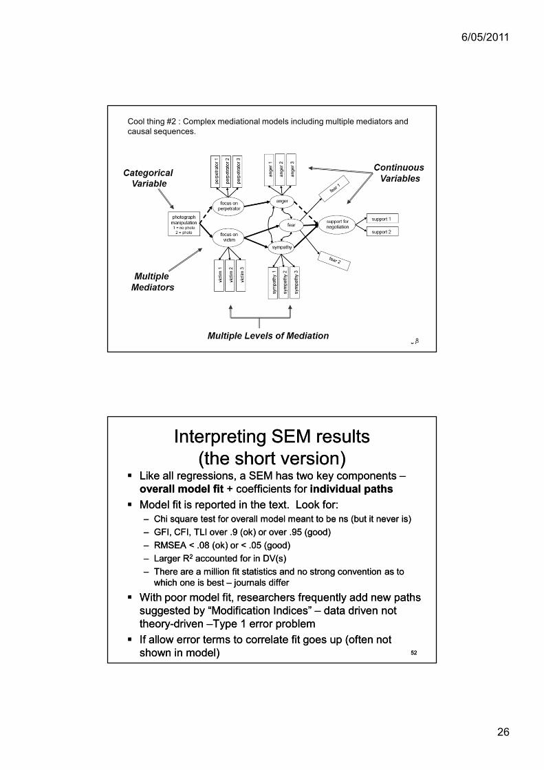
Cool thing #2 : Complex mediational models including multiple mediators and causal sequences.

Interpreting SEM resultsInterpreting SEM results(the short version)(the short version)

Like all regressions, a SEM has two key components Like all regressions, a SEM has two key components ––overall model fit overall model fit + coefficients for + coefficients for individual pathsindividual pathsModel fit is reported in the text. Look for:Model fit is reported in the text. Look for:–– Chi square test for overall model meant to be ns (but it never is)Chi square test for overall model meant to be ns (but it never is)–– GFI, CFI, TLI over .9 (ok) or over .95 (good)GFI, CFI, TLI over .9 (ok) or over .95 (good)–– RMSEA < .08 (ok) or < .05 (good)RMSEA < .08 (ok) or < .05 (good)–– Larger RLarger R22 accounted for in DV(s)accounted for in DV(s)–– There are a million fit statistics and no strong convention as to There are a million fit statistics and no strong convention as to

which one is best which one is best –– journals differjournals differ

With poor model fit, researchers frequently add new paths With poor model fit, researchers frequently add new paths suggested by “Modification Indices” suggested by “Modification Indices” –– data driven not data driven not theorytheory--driven driven ––Type 1 error problemType 1 error problemIf allow error terms to correlate fit goes up (often not If allow error terms to correlate fit goes up (often not shown in model)shown in model) 5252

6/05/2011

27

Direct and indirect effectsDirect and indirect effectsCoefficients for direct effects may be reported in text or Coefficients for direct effects may be reported in text or simply in figuresimply in figure–– You want significant coefficientsYou want significant coefficients–– But NB: whether it’s a unidirectional arrow in one direction, a biBut NB: whether it’s a unidirectional arrow in one direction, a bi--

directional arrow, or a unidirectional arrow in the other direction directional arrow, or a unidirectional arrow in the other direction is based on is based on theorytheory (causality is usually inferred)(causality is usually inferred)

Indirect effects generally reported in the text or a table. Indirect effects generally reported in the text or a table. In text “The indirect effect was significant (IE=.xx, In text “The indirect effect was significant (IE=.xx, UL=.xx, LL = .xx)”. UL=.xx, LL = .xx)”. –– IE is a coefficient for the indirect effect; UL and LL are upper and IE is a coefficient for the indirect effect; UL and LL are upper and

lower limit confidence intervals. Sig if UL to LL does not include lower limit confidence intervals. Sig if UL to LL does not include zero. E.g., UL= .15 LL = .03 is sig. UL = .15 LL = zero. E.g., UL= .15 LL = .03 is sig. UL = .15 LL = --.01 is ns..01 is ns.

In a full “effects decomposition” researchers report In a full “effects decomposition” researchers report estimates for the total effect (TE), direct effect (DE), and estimates for the total effect (TE), direct effect (DE), and indirect effect (IE) indirect effect (IE) –– generally in a Table.generally in a Table. 5353

A SEM A SEM writeupwriteup example excerpts from example excerpts from Barlow, Louis & Hewstone (2009)Barlow, Louis & Hewstone (2009)

The model provided a good fit to the data, The model provided a good fit to the data, x2(70, N = 272) = 136.30, p < .001, x2/x2(70, N = 272) = 136.30, p < .001, x2/dfdf = = 1.95; CFI = 0.98; RMSEA = .059; SRMR 1.95; CFI = 0.98; RMSEA = .059; SRMR =.061. The results of the present SEM are =.061. The results of the present SEM are displayed in Figure 1. A summary of the displayed in Figure 1. A summary of the effects decomposition analysis is shown in effects decomposition analysis is shown in Table 1.Table 1.

5454

6/05/2011

28

5555

Fig 1. Model stresses direct effect coefficients (always) plus R2 (not always).Note how the structural model is hidden here. Error terms also hidden.

5656

Table 1. Generally need to look at effects decomposition table along with figure. Note how multiple effects tested at once (exact ps hidden). Type 1 error avoided ostensibly by good model fit based on theory. No real effect sizes.

6/05/2011

29

Take home SEM messagesTake home SEM messagesSEM is a powerful technique that most readers, SEM is a powerful technique that most readers, reviewers, and researchers do not fully understandreviewers, and researchers do not fully understandSEM makes it possible to represent and test complex SEM makes it possible to represent and test complex causal models in a way that hides a lot of the mathcausal models in a way that hides a lot of the math–– Simultaneously awesome and disturbingSimultaneously awesome and disturbing

At its simplest, can be read like MR At its simplest, can be read like MR –– tells you (1) overall tells you (1) overall model fit; (2) relationships of predictors to DVsmodel fit; (2) relationships of predictors to DVsConventions still evolving; prone to confusion & misuseConventions still evolving; prone to confusion & misuse–– Common sins: (1) good model fit created by allowing error terms Common sins: (1) good model fit created by allowing error terms

to correlate (hidden off figure); (2) dodgy ‘itemto correlate (hidden off figure); (2) dodgy ‘item--parcelling’ to avoid parcelling’ to avoid bad fit in structural model; (3) paths added based on modification bad fit in structural model; (3) paths added based on modification indices (dataindices (data--driven driven –– may not replicate)may not replicate)

5757

5858

In class next week:In class next week:Within Ps ANOVAWithin Ps ANOVA

In the tutes:In the tutes:This week: This week: Feedback on A1 + Tips on A2Feedback on A1 + Tips on A2Next week: Consult for A2Next week: Consult for A2

Readings :Readings :HowellHowell–– chapter 14chapter 14

FieldField–– Chapter 11Chapter 11

Documents

Quiz 2 next Sunday & Monday