QUEST User Manual

Yu-Shan ShihDepartment of Mathematics

National Chung Cheng University, Taiwanyshih@math.ccu.edu.tw

Revised April 27, 2004

Contents

1 Introduction 1

2 Distribution files 22.1 Library files . . . . . . . . . . . . . . . . . . . . . . . . . . . . . . . . . . . . . . . . . . . 2

3 Input files 33.1 Data file . . . . . . . . . . . . . . . . . . . . . . . . . . . . . . . . . . . . . . . . . . . . . 33.2 Description file . . . . . . . . . . . . . . . . . . . . . . . . . . . . . . . . . . . . . . . . . 3

4 Running the program 44.1 Interactive mode . . . . . . . . . . . . . . . . . . . . . . . . . . . . . . . . . . . . . . . . 44.2 Explanation of questions . . . . . . . . . . . . . . . . . . . . . . . . . . . . . . . . . . . . 74.3 Batch mode . . . . . . . . . . . . . . . . . . . . . . . . . . . . . . . . . . . . . . . . . . . 8

5 Sample output files 85.1 Annotated output . . . . . . . . . . . . . . . . . . . . . . . . . . . . . . . . . . . . . . . . 95.2 Explanation of annotations . . . . . . . . . . . . . . . . . . . . . . . . . . . . . . . . . . . 185.3 Linear combination splits . . . . . . . . . . . . . . . . . . . . . . . . . . . . . . . . . . . . 20

1 Introduction

QUEST stands for “Quick, Unbiased, Efficient Statistical Trees” and is a program for tree-structured classi-fication. The algorithms are described in Loh and Shih (1997). The performance of QUEST comparedwith other classification methods can be found in Lim, Loh and Shih (2000). The main strengths ofQUEST are unbiased variable selection and fast computational speed. In addition, it has options to performCART-style exhaustive search and cost-complexity cross-validation pruning (Breiman, Friedman, Olshenand Stone, 1984). This version is coded in Fortran 90. The main changes since version 1.6 are

1. an option to handle missing values is included,

2. linear combination split for mixed variables is added,

1

3. exhaustive search method is added for split point selection,

4. family of splitting criteria is added,

5. dynamic allocation of memory is used,

6. an interactive mode is added into the main program,

7. options related to direct stopping, importance ranking, deviance pruning and global CV are dropped.

The updated versions of QUEST can be obtained from

http://www.stat.wisc.edu/∼loh/quest.html.

For detailed changes made in the latest version, please read the companion history file: history.txt. This usermanual explains how the program is executed and how the output is interpreted.

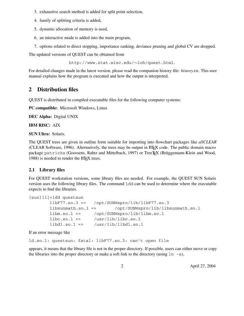
2 Distribution files

QUEST is distributed in compiled executable files for the following computer systems:

PC compatible: Microsoft Windows, Linux

DEC Alpha: Digital UNIX

IBM RISC: AIX

SUN Ultra: Solaris.

The QUEST trees are given in outline form suitable for importing into flowchart packages like allCLEAR(CLEAR Software, 1996). Alternatively, the trees may be output in LATEX code. The public domain macropackage pstricks (Goossens, Rahtz and Mittelbach, 1997) or TreeTEX (Bruggemann-Klein and Wood,1988) is needed to render the LATEX trees.

2.1 Library files

For QUEST workstation versions, some library files are needed. For example, the QUEST SUN Solarisversion uses the following library files. The command ldd can be used to determine where the executableexpects to find the libraries.

[sun][1]>ldd questsunlibF77.so.3 => /opt/SUNWspro/lib/libF77.so.3libsunmath.so.1 => /opt/SUNWspro/lib/libsunmath.so.1libm.so.1 => /opt/SUNWspro/lib/libm.so.1libc.so.1 => /usr/lib/libc.so.1libdl.so.1 => /usr/lib/libdl.so.1

If an error message like

ld.so.1: questsun: fatal: libF77.so.3: can’t open file

appears, it means that the library file is not in the proper directory. If possible, users can either move or copythe libraries into the proper directory or make a soft link to the directory (using ln -s).

2 April 27, 2004

3 Input files

The QUEST program needs two text input files.

3.1 Data file

This file contains the learning (or training) samples. Each sample consists of observations on the class (orresponse or dependent) variable and the predictor (or independent) variables plus any frequency variable.The entries in each sample record should be comma or space delimited. Each record can occupy one ormore lines in the file, but each record must begin on a new line. Record values can be numerical or characterstrings. Categorical variables can be given numerical or character values. Any character string that containsa comma or space must be surrounded by a matching pair of quotation marks (either ’ or "). Please makesure that either the data file or the description file ends with a carriage return. Otherwise, the program willignore all incomplete lines and may yield false results.

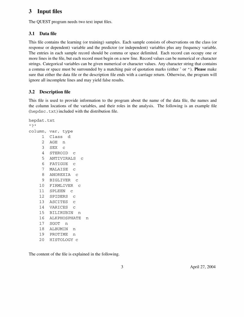
3.2 Description file

This file is used to provide information to the program about the name of the data file, the names andthe column locations of the variables, and their roles in the analysis. The following is an example file(hepdsc.txt) included with the distribution file.

hepdat.txt"?"column, var, type

1 Class d2 AGE n3 SEX c4 STEROID c5 ANTIVIRALS c6 FATIGUE c7 MALAISE c8 ANOREXIA c9 BIGLIVER c

10 FIRMLIVER c11 SPLEEN c12 SPIDERS c13 ASCITES c14 VARICES c15 BILIRUBIN n16 ALKPHOSPHATE n17 SGOT n18 ALBUMIN n19 PROTIME n20 HISTOLOGY c

The content of the file is explained in the following.

3 April 27, 2004

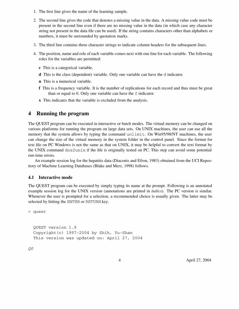
1. The first line gives the name of the learning sample.

2. The second line gives the code that denotes a missing value in the data. A missing value code must bepresent in the second line even if there are no missing value in the data (in which case any characterstring not present in the data file can be used). If the string contains characters other than alphabets ornumbers, it must be surrounded by quotation marks.

3. The third line contains three character strings to indicate column headers for the subsequent lines.

4. The position, name and role of each variable comes next with one line for each variable. The followingroles for the variables are permitted:

c This is a categorical variable.

d This is the class (dependent) variable. Only one variable can have the d indicator.

n This is a numerical variable.

f This is a frequency variable. It is the number of replications for each record and thus must be greatthan or equal to 0. Only one variable can have the f indicator.

x This indicates that the variable is excluded from the analysis.

4 Running the program

The QUEST program can be executed in interactive or batch modes. The virtual memory can be changed onvarious platforms for running the program on large data sets. On UNIX machines, the user can use all thememory that the system allows by typing the command unlimit. On Win95/98/NT machines, the usercan change the size of the virtual memory in the system folder in the control panel. Since the format fortext file on PC Windows is not the same as that on UNIX, it may be helpful to convert the text format bythe UNIX command dos2unix if the file is originally tested on PC. This step can avoid some potentialrun-time errors.

An example session log for the hepatitis data (Diaconis and Efron, 1983) obtained from the UCI Repos-itory of Machine Learning Databases (Blake and Merz, 1998) follows.

4.1 Interactive mode

The QUEST program can be executed by simply typing its name at the prompt. Following is an annotatedexample session log for the UNIX version (annotations are printed in italics). The PC version is similar.Whenever the user is prompted for a selection, a recommended choice is usually given. The latter may beselected by hitting the ENTER or RETURN key.

> quest

QUEST version 1.9Copyright(c) 1997-2004 by Shih, Yu-ShanThis version was updated on: April 27, 2004

Q0

4 April 27, 2004

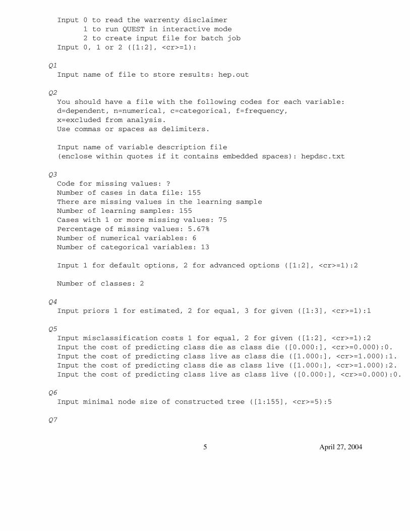
Input 0 to read the warrenty disclaimer1 to run QUEST in interactive mode2 to create input file for batch job

Input 0, 1 or 2 ([1:2], <cr>=1):

Q1Input name of file to store results: hep.out

Q2You should have a file with the following codes for each variable:d=dependent, n=numerical, c=categorical, f=frequency,x=excluded from analysis.Use commas or spaces as delimiters.

Input name of variable description file(enclose within quotes if it contains embedded spaces): hepdsc.txt

Q3Code for missing values: ?Number of cases in data file: 155There are missing values in the learning sampleNumber of learning samples: 155Cases with 1 or more missing values: 75Percentage of missing values: 5.67%Number of numerical variables: 6Number of categorical variables: 13

Input 1 for default options, 2 for advanced options ([1:2], <cr>=1):2

Number of classes: 2

Q4Input priors 1 for estimated, 2 for equal, 3 for given ([1:3], <cr>=1):1

Q5Input misclassification costs 1 for equal, 2 for given ([1:2], <cr>=1):2Input the cost of predicting class die as class die ([0.000:], <cr>=0.000):0.Input the cost of predicting class live as class die ([1.000:], <cr>=1.000):1.Input the cost of predicting class die as class live ([1.000:], <cr>=1.000):2.Input the cost of predicting class live as class live ([0.000:], <cr>=0.000):0.

Q6Input minimal node size of constructed tree ([1:155], <cr>=5):5

Q7

5 April 27, 2004

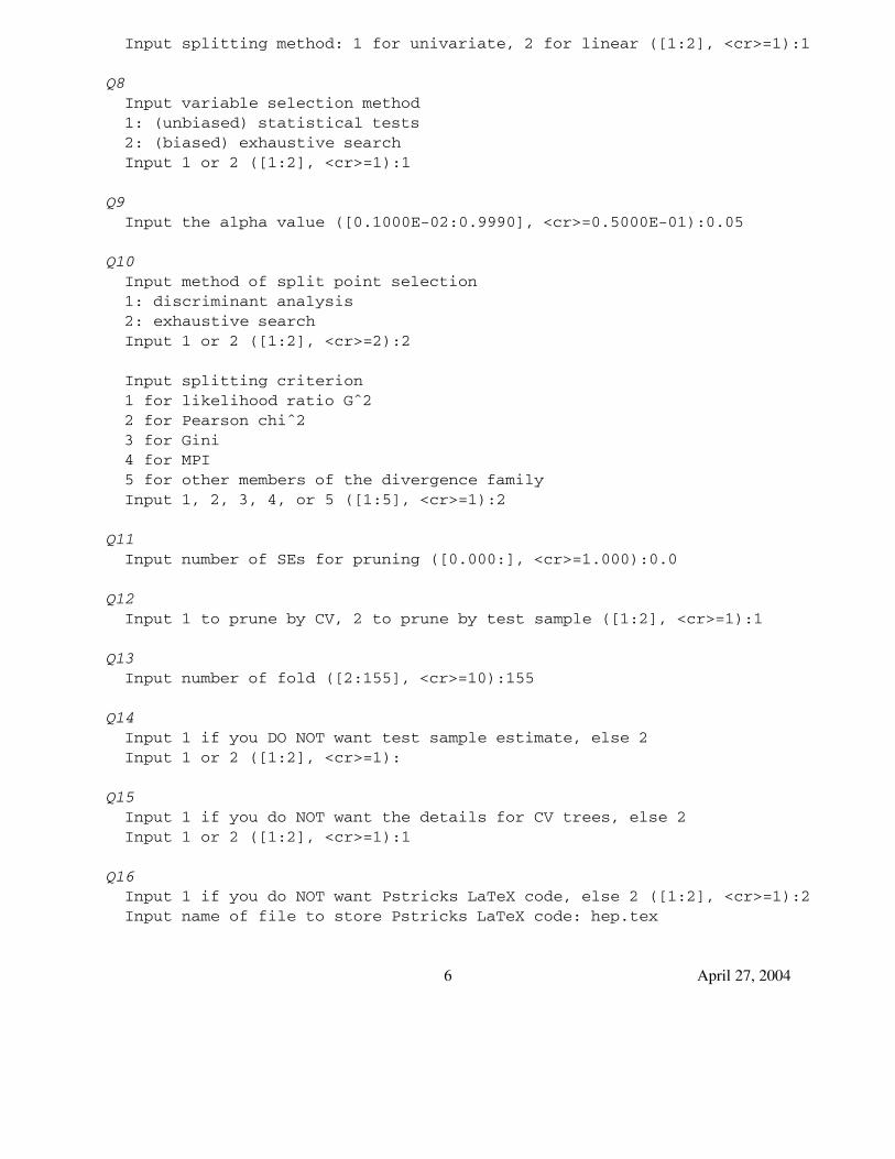
Input splitting method: 1 for univariate, 2 for linear ([1:2], <cr>=1):1

Q8Input variable selection method1: (unbiased) statistical tests2: (biased) exhaustive searchInput 1 or 2 ([1:2], <cr>=1):1

Q9Input the alpha value ([0.1000E-02:0.9990], <cr>=0.5000E-01):0.05

Q10Input method of split point selection1: discriminant analysis2: exhaustive searchInput 1 or 2 ([1:2], <cr>=2):2

Input splitting criterion1 for likelihood ratio Gˆ22 for Pearson chiˆ23 for Gini4 for MPI5 for other members of the divergence familyInput 1, 2, 3, 4, or 5 ([1:5], <cr>=1):2

Q11Input number of SEs for pruning ([0.000:], <cr>=1.000):0.0

Q12Input 1 to prune by CV, 2 to prune by test sample ([1:2], <cr>=1):1

Q13Input number of fold ([2:155], <cr>=10):155

Q14Input 1 if you DO NOT want test sample estimate, else 2Input 1 or 2 ([1:2], <cr>=1):

Q15Input 1 if you do NOT want the details for CV trees, else 2Input 1 or 2 ([1:2], <cr>=1):1

Q16Input 1 if you do NOT want Pstricks LaTeX code, else 2 ([1:2], <cr>=1):2Input name of file to store Pstricks LaTeX code: hep.tex

6 April 27, 2004

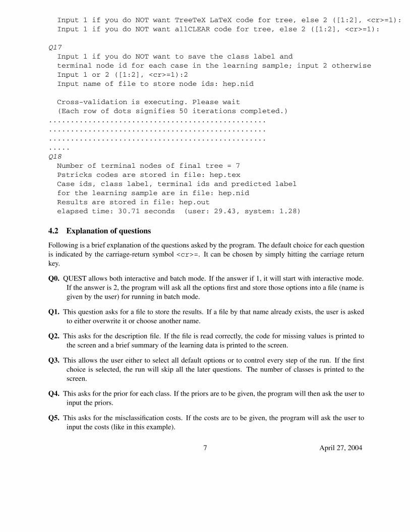
Input 1 if you do NOT want TreeTeX LaTeX code for tree, else 2 ([1:2], <cr>=1):Input 1 if you do NOT want allCLEAR code for tree, else 2 ([1:2], <cr>=1):

Q17Input 1 if you do NOT want to save the class label andterminal node id for each case in the learning sample; input 2 otherwiseInput 1 or 2 ([1:2], <cr>=1):2Input name of file to store node ids: hep.nid

Cross-validation is executing. Please wait(Each row of dots signifies 50 iterations completed.)

..................................................

..................................................

..................................................

.....Q18

Number of terminal nodes of final tree = 7Pstricks codes are stored in file: hep.texCase ids, class label, terminal ids and predicted labelfor the learning sample are in file: hep.nidResults are stored in file: hep.outelapsed time: 30.71 seconds (user: 29.43, system: 1.28)

4.2 Explanation of questions

Following is a brief explanation of the questions asked by the program. The default choice for each questionis indicated by the carriage-return symbol <cr>=. It can be chosen by simply hitting the carriage returnkey.

Q0. QUEST allows both interactive and batch mode. If the answer if 1, it will start with interactive mode.If the answer is 2, the program will ask all the options first and store those options into a file (name isgiven by the user) for running in batch mode.

Q1. This question asks for a file to store the results. If a file by that name already exists, the user is askedto either overwrite it or choose another name.

Q2. This asks for the description file. If the file is read correctly, the code for missing values is printed tothe screen and a brief summary of the learning data is printed to the screen.

Q3. This allows the user either to select all default options or to control every step of the run. If the firstchoice is selected, the run will skip all the later questions. The number of classes is printed to thescreen.

Q4. This asks for the prior for each class. If the priors are to be given, the program will then ask the user toinput the priors.

Q5. This asks for the misclassification costs. If the costs are to be given, the program will ask the user toinput the costs (like in this example).

7 April 27, 2004

Q6. This asks for the smallest number of samples in a node during tree construction. A node will not besplit if it contains fewer cases than this number. The smaller this value is, the larger the initial tree willbe prior to pruning. The default value is max(5, n/100), where n is the total number of observations.

Q7. The user can choose either splits on single variable or linear combination of variables.

Q8. This asks for the user to choose between the unbiased variable selection method described in Loh andShih (1997) or the biased exhaustive search method which is used in CART.

Q9. If the unbiased method based on statistical tests is used in Q8, this asks for the alpha value to conductthe tests. The suggest value is usually best.

Q10. For the split point, this asks for the user to choose between methods using discriminant analysis (Lohand Shih, 1997) and the exhaustive search method (Breiman et al., 1984). The former is the defaultoption if the number of classes is more than 2, otherwise the latter is the default option. If the latteroption is selected, the program will ask for the user to choose the splitting criterion. These criteria arestudied in Shih (1999). The likelihood criterion is the default option. If instead the CART-style splitis used, the Gini criterion is the default option.

Q11. The number of SEs controls the size of the pruned tree. 0-SE gives the tree with the smallest cross-validation estimate of misclassification cost or error.

Q12. The user can choose to select the final tree by cross-validation or test sample pruning. Test sampleestimates are available for both trees.

Q13. This asks for the value of V in V-fold cross-validation. The larger the value of V is, the longer runningtime the program takes. 10-fold is usually recommended and is the default in CART.

Q14. The test sample estimate can be obtained for the final CV tree, if it is needed.

Q15. The details of CV tree sequences are reported, if the user chooses 2. They are not reported by default.

Q16. If LATEX source code for drawing the tree is needed, the user should choose 2 to use either pstricksor TreeTEX package. So is allCLEAR code.

Q17. This allows the user to obtain a file containing the class label and terminal node for each case inthe learning sample. The information is useful for extracting the learning samples from particularterminal nodes of the tree.

Q18. After the tree is built, some related information is printed to the screen.

4.3 Batch mode

If the answer in Q0 is 2, QUEST will ask for a file to store the selected options. It also checks the descriptionfile and the data file. However, it does not construct the tree. After all the questions being asked, QUESTwill prompt the command for running a job in batch mode.

5 Sample output files

The annotated output file hep.out is in the following.

8 April 27, 2004

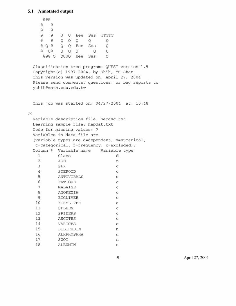
5.1 Annotated output

@@@@ @@ @@ @ U U Eee Sss TTTTT@ @ Q Q Q Q Q@ Q @ Q Q Eee Sss Q@ Q@ Q Q Q Q Q@@@ Q QUUQ Eee Sss Q

Classification tree program: QUEST version 1.9Copyright(c) 1997-2004, by Shih, Yu-ShanThis version was updated on: April 27, 2004Please send comments, questions, or bug reports toyshih@math.ccu.edu.tw

This job was started on: 04/27/2004 at: 10:48

P1Variable description file: hepdsc.txtLearning sample file: hepdat.txtCode for missing values: ?Variables in data file are(variable types are d=dependent, n=numerical,c=categorical, f=frequency, x=excluded):

Column # Variable name Variable type1 Class d2 AGE n3 SEX c4 STEROID c5 ANTIVIRALS c6 FATIGUE c7 MALAISE c8 ANOREXIA c9 BIGLIVER c

10 FIRMLIVER c11 SPLEEN c12 SPIDERS c13 ASCITES c14 VARICES c15 BILIRUBIN n16 ALKPHOSPHA n17 SGOT n18 ALBUMIN n

9 April 27, 2004

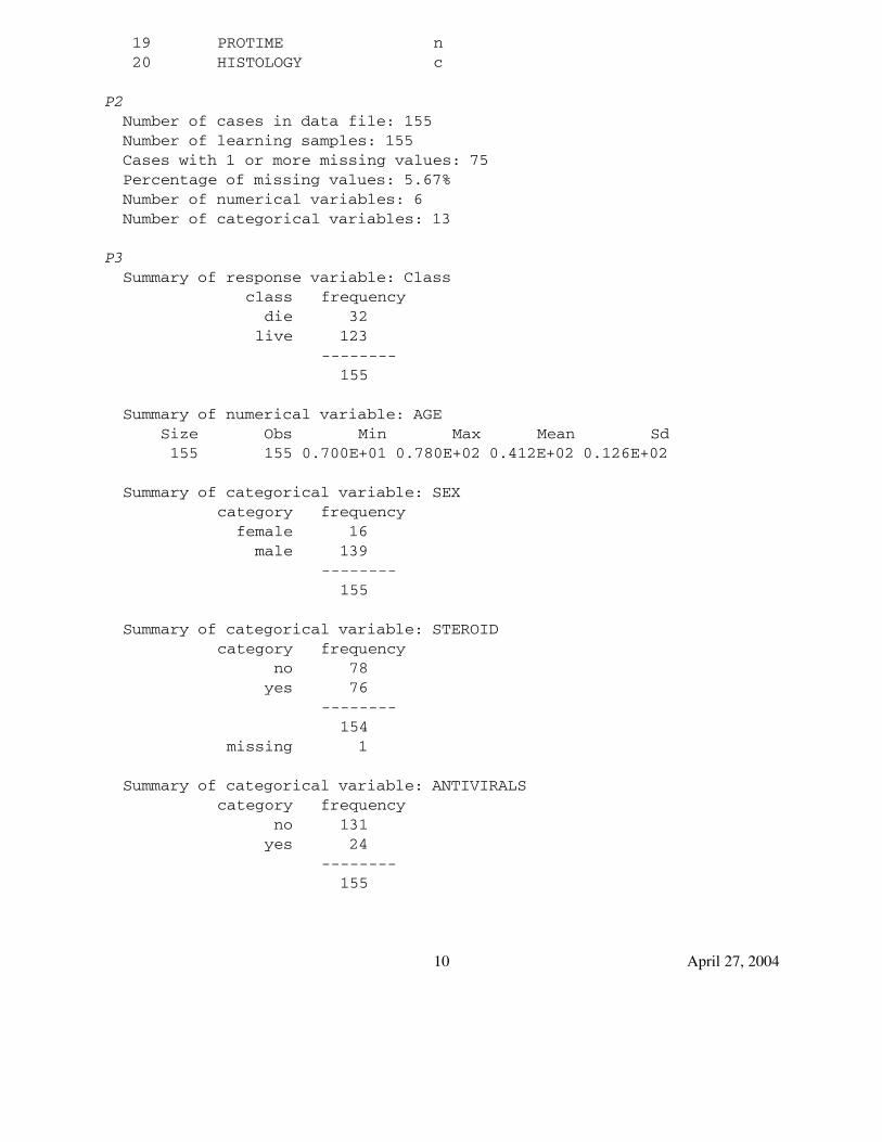
19 PROTIME n20 HISTOLOGY c

P2Number of cases in data file: 155Number of learning samples: 155Cases with 1 or more missing values: 75Percentage of missing values: 5.67%Number of numerical variables: 6Number of categorical variables: 13

P3Summary of response variable: Class

class frequencydie 32

live 123--------

155

Summary of numerical variable: AGESize Obs Min Max Mean Sd155 155 0.700E+01 0.780E+02 0.412E+02 0.126E+02

Summary of categorical variable: SEXcategory frequency

female 16male 139

--------155

Summary of categorical variable: STEROIDcategory frequency

no 78yes 76

--------154

missing 1

Summary of categorical variable: ANTIVIRALScategory frequency

no 131yes 24

--------155

10 April 27, 2004

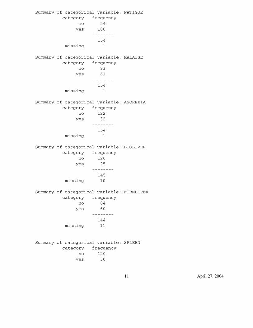
Summary of categorical variable: FATIGUEcategory frequency

no 54yes 100

--------154

missing 1

Summary of categorical variable: MALAISEcategory frequency

no 93yes 61

--------154

missing 1

Summary of categorical variable: ANOREXIAcategory frequency

no 122yes 32

--------154

missing 1

Summary of categorical variable: BIGLIVERcategory frequency

no 120yes 25

--------145

missing 10

Summary of categorical variable: FIRMLIVERcategory frequency

no 84yes 60

--------144

missing 11

Summary of categorical variable: SPLEENcategory frequency

no 120yes 30

11 April 27, 2004

--------150

missing 5

Summary of categorical variable: SPIDERScategory frequency

no 99yes 51

--------150

missing 5

Summary of categorical variable: ASCITEScategory frequency

no 130yes 20

--------150

Summary of categorical variable: VARICEScategory frequency

no 132yes 18

--------150

missing 5

Summary of numerical variable: BILIRUBINSize Obs Min Max Mean Sd155 149 0.300E+00 0.800E+01 0.143E+01 0.121E+01

Summary of numerical variable: ALKPHOSPHATESize Obs Min Max Mean Sd155 126 0.260E+02 0.295E+03 0.105E+03 0.515E+02

Summary of numerical variable: SGOTSize Obs Min Max Mean Sd155 151 0.140E+02 0.648E+03 0.859E+02 0.897E+02

Summary of numerical variable: ALBUMINSize Obs Min Max Mean Sd155 139 0.210E+01 0.640E+01 0.382E+01 0.652E+00

Summary of numerical variable: PROTIMESize Obs Min Max Mean Sd

12 April 27, 2004

155 88 0.000E+00 0.100E+03 0.619E+02 0.229E+02

Summary of categorical variable: HISTOLOGYcategory frequency

no 85yes 70

--------155

Options for tree constructionestimated priors are

Class priordie 0.20645

live 0.79355The cost matrix is in the following formatcost(1|1),cost(1|2),.....,cost(1|no. of class)cost(2|1),cost(2|2),.....,cost(2|no. of class)............................................................................................cost(no. of class|1),.. .,cost(no. of class|no. of class)where cost(i|j)= cost of misclassifying class jas class i and class label is assigned in alphabetical order

0.0000000E+00 1.0000002.000000 0.0000000E+00

The altered priors aredie:.34225

live:.65775

P4minimal node size: 5use univariate splituse (unbiased) statistical tests for variable selectionalpha value: .050split point method: exhaustive searchuse Pearson chiˆ2

P5use 155-fold CV sample pruningSE-rule trees based on number of SEs = 0.00

P6subtree # Terminal complexity currentnumber nodes value cost

1 15 0.0000 0.0581

13 April 27, 2004

2 9 0.0043 0.08393 8 0.0065 0.09034 7 0.0129 0.10325 2 0.0284 0.24526 1 0.1677 0.4129

P7Size and CV misclassification cost and SE of subtrees:Tree #Tnodes Mean SE(Mean)

1 15 0.3355 0.4937E-012 9 0.3419 0.5034E-013 8 0.3290 0.5089E-014** 7 0.2903 0.4911E-015 2 0.3226 0.4556E-016 1 0.4129 0.6502E-01

CART 0-SE tree is marked with *CART SE-rule using CART SE is marked with **The * and ** trees are the same

P8Following tree is based on *

Structure of final tree

Node Left node Right node Split variable Predicted class1 2 3 ALBUMIN2 4 5 BILIRUBIN4 6 7 ASCITES6 8 9 MALAISE8 * terminal node * live9 14 15 STEROID

14 * terminal node * live15 16 17 PROTIME16 * terminal node * die17 * terminal node * live7 * terminal node * die5 * terminal node * die3 * terminal node * live

Number of terminal nodes of final tree = 7Total number of nodes of final tree = 13

P9

14 April 27, 2004

Classification tree:

Node 1: ALBUMIN <= 3.850Node 2: BILIRUBIN <= 3.700

Node 4: ASCITES = noNode 6: MALAISE = no

Node 8: liveNode 6: MALAISE = yes

Node 9: STEROID = noNode 14: live

Node 9: STEROID = yesNode 15: PROTIME <= 70.50

Node 16: dieNode 15: PROTIME > 70.50

Node 17: liveNode 4: ASCITES = yes

Node 7: dieNode 2: BILIRUBIN > 3.700

Node 5: dieNode 1: ALBUMIN > 3.850

Node 3: live

P10Information for each node:

**************************************************Node 1: Intermediate nodeA case goes into Node 2 if its value of ALBUMIN <= 3.8500

Class # cases Mean of ALBUMINdie 32 3.1519

live 123 3.9777--------

155

**************************************************Node 2: Intermediate nodeA case goes into Node 4 if its value of BILIRUBIN <= 3.7000

Class # cases Mean of BILIRUBINdie 29 2.6222

live 32 1.3687--------

61

**************************************************Node 4: Intermediate nodeA case goes into Node 6 if its value of ASCITES =

15 April 27, 2004

noClass # cases Mode of ASCITESdie 21 no

live 32 no--------

53

**************************************************Node 6: Intermediate nodeA case goes into Node 8 if its value of MALAISE =

noClass # cases Mode of MALAISEdie 12 yes

live 28 no--------

40

**************************************************Node 8: Terminal node assigned to Class live

Class # casesdie 3

live 18-------

21

**************************************************Node 9: Intermediate nodeA case goes into Node 14 if its value of STEROID =

noClass # cases Mode of STEROIDdie 9 yes

live 10 yes--------

19

**************************************************Node 14: Terminal node assigned to Class live

Class # casesdie 0

live 4-------

4

**************************************************Node 15: Intermediate nodeA case goes into Node 16 if its value of PROTIME <= 70.500

Class # cases Mean of PROTIMEdie 9 36.333

live 6 100.00

16 April 27, 2004

--------15

**************************************************Node 16: Terminal node assigned to Class die

Class # casesdie 9

live 0-------

9

**************************************************Node 17: Terminal node assigned to Class live

Class # casesdie 0

live 6-------

6

**************************************************Node 7: Terminal node assigned to Class die

Class # casesdie 9

live 4-------

13

**************************************************Node 5: Terminal node assigned to Class die

Class # casesdie 8

live 0-------

8

**************************************************Node 3: Terminal node assigned to Class live

Class # casesdie 3

live 91-------

94P11Classification matrix based on learning sample

predicted classactual class die live

die 26 6live 4 119

Classification matrix based on 155-fold CV

17 April 27, 2004

predicted classactual class die live

die 19 13live 19 104

P12Pstricks codes are stored in file: hep.tex

Case ids, class label, terminal ids and predicted labelfor the learning sample are in file: hep.nid

elapsed time: 30.71 seconds (user: 29.43, system: 1.28)

This job was completed on: 04/27/2004 at: 10:49

5.2 Explanation of annotations

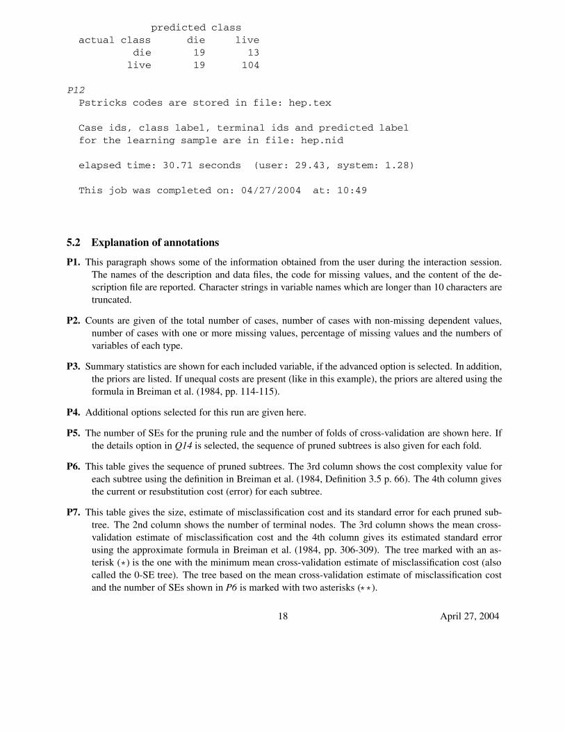
P1. This paragraph shows some of the information obtained from the user during the interaction session.The names of the description and data files, the code for missing values, and the content of the de-scription file are reported. Character strings in variable names which are longer than 10 characters aretruncated.

P2. Counts are given of the total number of cases, number of cases with non-missing dependent values,number of cases with one or more missing values, percentage of missing values and the numbers ofvariables of each type.

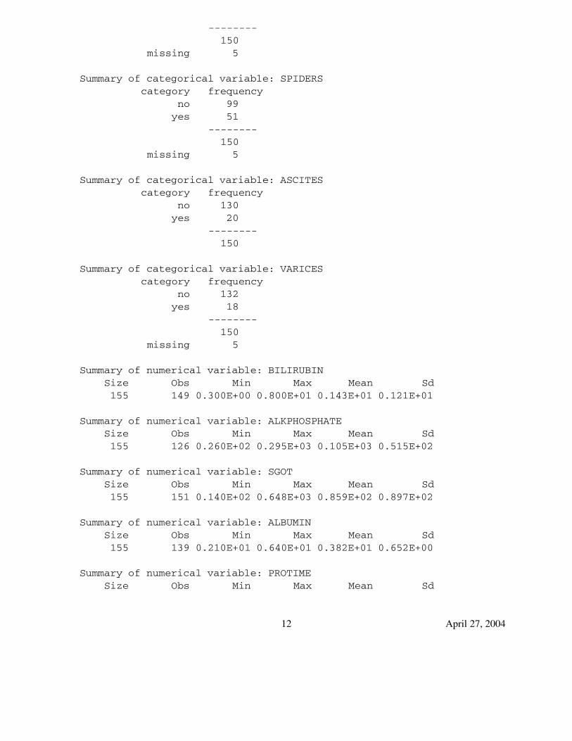
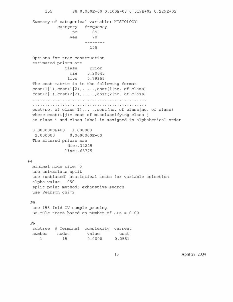
P3. Summary statistics are shown for each included variable, if the advanced option is selected. In addition,the priors are listed. If unequal costs are present (like in this example), the priors are altered using theformula in Breiman et al. (1984, pp. 114-115).

P4. Additional options selected for this run are given here.

P5. The number of SEs for the pruning rule and the number of folds of cross-validation are shown here. Ifthe details option in Q14 is selected, the sequence of pruned subtrees is also given for each fold.

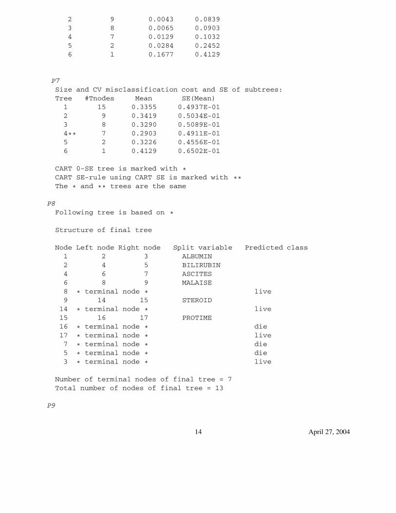
P6. This table gives the sequence of pruned subtrees. The 3rd column shows the cost complexity value foreach subtree using the definition in Breiman et al. (1984, Definition 3.5 p. 66). The 4th column givesthe current or resubstitution cost (error) for each subtree.

P7. This table gives the size, estimate of misclassification cost and its standard error for each pruned sub-tree. The 2nd column shows the number of terminal nodes. The 3rd column shows the mean cross-validation estimate of misclassification cost and the 4th column gives its estimated standard errorusing the approximate formula in Breiman et al. (1984, pp. 306-309). The tree marked with an as-terisk (*) is the one with the minimum mean cross-validation estimate of misclassification cost (alsocalled the 0-SE tree). The tree based on the mean cross-validation estimate of misclassification costand the number of SEs shown in P6 is marked with two asterisks (**).

18 April 27, 2004

P8. The structure of the tree selected by the user (the tree marked by** in this example) is given here. Theroot node always has the label 1. The total number of nodes and terminal nodes are also shown.

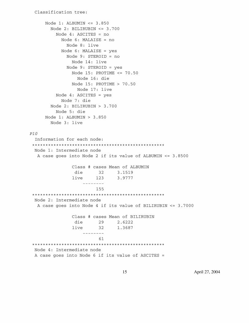
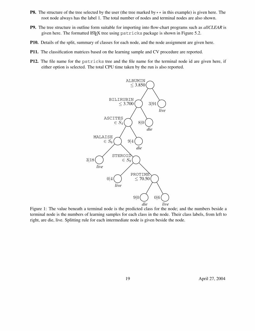
P9. The tree structure in outline form suitable for importing into flow-chart programs such as allCLEAR isgiven here. The formatted LATEX tree using pstricks package is shown in Figure 5.2.

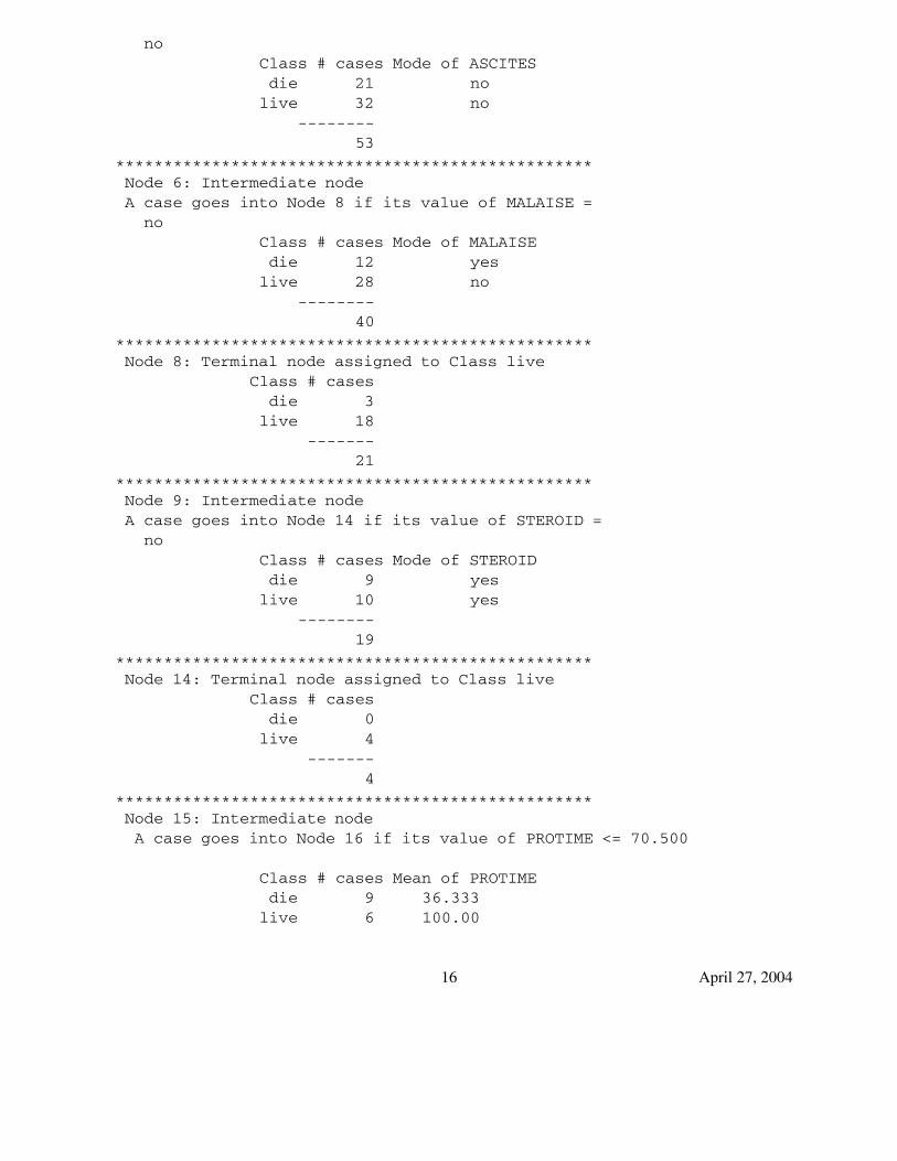
P10. Details of the split, summary of classes for each node, and the node assignment are given here.

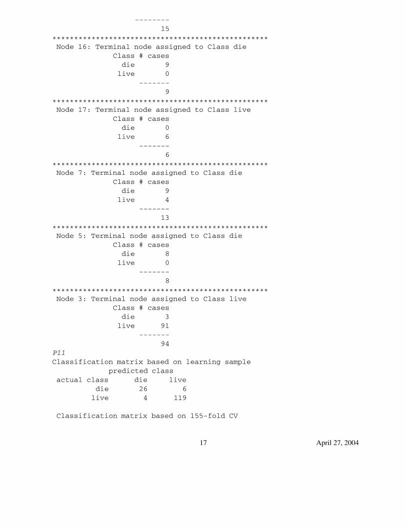
P11. The classification matrices based on the learning sample and CV procedure are reported.

P12. The file name for the pstricks tree and the file name for the terminal node id are given here, ifeither option is selected. The total CPU time taken by the run is also reported.

ALBUMIN≤ 3.850

BILIRUBIN≤ 3.700

ASCITES∈ S4

MALAISE∈ S6

3|18live

STEROID∈ S9

0|4live

PROTIME≤ 70.50

9|0die

0|6live

9|4die

8|0die

3|91live

Figure 1: The value beneath a terminal node is the predicted class for the node; and the numbers beside aterminal node is the numbers of learning samples for each class in the node. Their class labels, from left toright, are die, live. Splitting rule for each intermediate node is given beside the node.

19 April 27, 2004

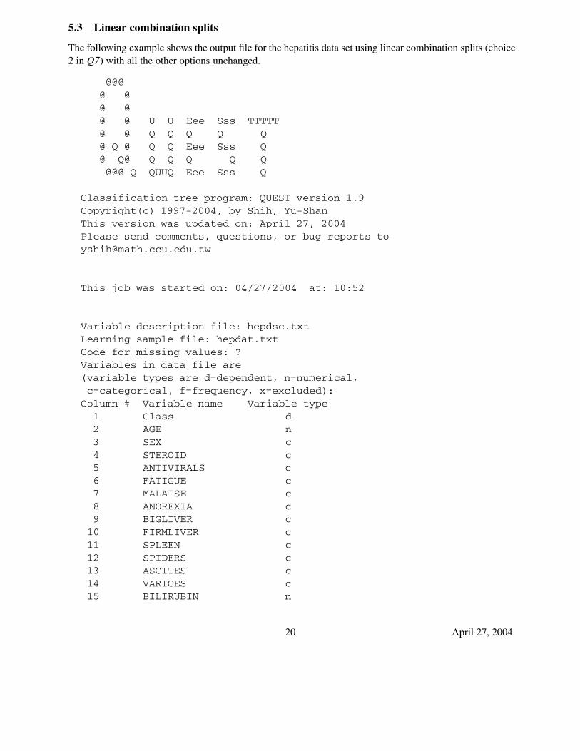
5.3 Linear combination splits

The following example shows the output file for the hepatitis data set using linear combination splits (choice2 in Q7) with all the other options unchanged.

@@@@ @@ @@ @ U U Eee Sss TTTTT@ @ Q Q Q Q Q@ Q @ Q Q Eee Sss Q@ Q@ Q Q Q Q Q@@@ Q QUUQ Eee Sss Q

Classification tree program: QUEST version 1.9Copyright(c) 1997-2004, by Shih, Yu-ShanThis version was updated on: April 27, 2004Please send comments, questions, or bug reports toyshih@math.ccu.edu.tw

This job was started on: 04/27/2004 at: 10:52

Variable description file: hepdsc.txtLearning sample file: hepdat.txtCode for missing values: ?Variables in data file are(variable types are d=dependent, n=numerical,c=categorical, f=frequency, x=excluded):

Column # Variable name Variable type1 Class d2 AGE n3 SEX c4 STEROID c5 ANTIVIRALS c6 FATIGUE c7 MALAISE c8 ANOREXIA c9 BIGLIVER c

10 FIRMLIVER c11 SPLEEN c12 SPIDERS c13 ASCITES c14 VARICES c15 BILIRUBIN n

20 April 27, 2004

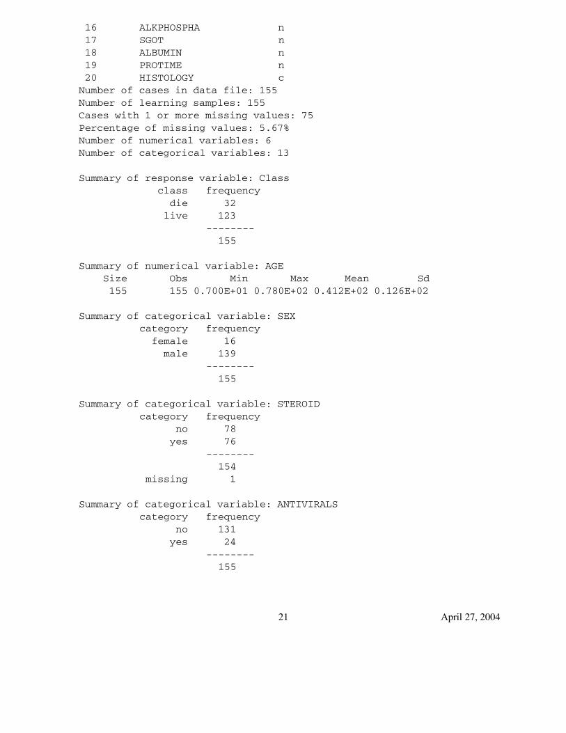
16 ALKPHOSPHA n17 SGOT n18 ALBUMIN n19 PROTIME n20 HISTOLOGY c

Number of cases in data file: 155Number of learning samples: 155Cases with 1 or more missing values: 75Percentage of missing values: 5.67%Number of numerical variables: 6Number of categorical variables: 13

Summary of response variable: Classclass frequency

die 32live 123

--------155

Summary of numerical variable: AGESize Obs Min Max Mean Sd155 155 0.700E+01 0.780E+02 0.412E+02 0.126E+02

Summary of categorical variable: SEXcategory frequency

female 16male 139

--------155

Summary of categorical variable: STEROIDcategory frequency

no 78yes 76

--------154

missing 1

Summary of categorical variable: ANTIVIRALScategory frequency

no 131yes 24

--------155

21 April 27, 2004

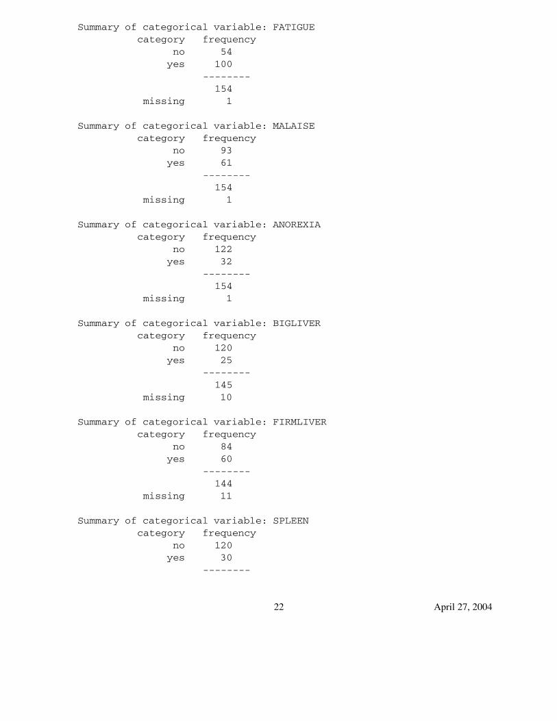
Summary of categorical variable: FATIGUEcategory frequency

no 54yes 100

--------154

missing 1

Summary of categorical variable: MALAISEcategory frequency

no 93yes 61

--------154

missing 1

Summary of categorical variable: ANOREXIAcategory frequency

no 122yes 32

--------154

missing 1

Summary of categorical variable: BIGLIVERcategory frequency

no 120yes 25

--------145

missing 10

Summary of categorical variable: FIRMLIVERcategory frequency

no 84yes 60

--------144

missing 11

Summary of categorical variable: SPLEENcategory frequency

no 120yes 30

--------

22 April 27, 2004

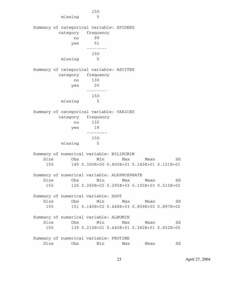
150missing 5

Summary of categorical variable: SPIDERScategory frequency

no 99yes 51

--------150

missing 5

Summary of categorical variable: ASCITEScategory frequency

no 130yes 20

--------150

missing 5

Summary of categorical variable: VARICEScategory frequency

no 132yes 18

--------150

missing 5

Summary of numerical variable: BILIRUBINSize Obs Min Max Mean Sd155 149 0.300E+00 0.800E+01 0.143E+01 0.121E+01

Summary of numerical variable: ALKPHOSPHATESize Obs Min Max Mean Sd155 126 0.260E+02 0.295E+03 0.105E+03 0.515E+02

Summary of numerical variable: SGOTSize Obs Min Max Mean Sd155 151 0.140E+02 0.648E+03 0.859E+02 0.897E+02

Summary of numerical variable: ALBUMINSize Obs Min Max Mean Sd155 139 0.210E+01 0.640E+01 0.382E+01 0.652E+00

Summary of numerical variable: PROTIMESize Obs Min Max Mean Sd

23 April 27, 2004

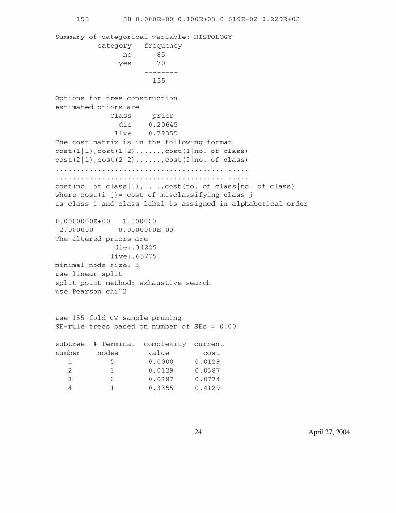
155 88 0.000E+00 0.100E+03 0.619E+02 0.229E+02

Summary of categorical variable: HISTOLOGYcategory frequency

no 85yes 70

--------155

Options for tree constructionestimated priors are

Class priordie 0.20645

live 0.79355The cost matrix is in the following formatcost(1|1),cost(1|2),.....,cost(1|no. of class)cost(2|1),cost(2|2),.....,cost(2|no. of class)............................................................................................cost(no. of class|1),.. .,cost(no. of class|no. of class)where cost(i|j)= cost of misclassifying class jas class i and class label is assigned in alphabetical order

0.0000000E+00 1.0000002.000000 0.0000000E+00

The altered priors aredie:.34225

live:.65775minimal node size: 5use linear splitsplit point method: exhaustive searchuse Pearson chiˆ2

use 155-fold CV sample pruningSE-rule trees based on number of SEs = 0.00

subtree # Terminal complexity currentnumber nodes value cost

1 5 0.0000 0.01292 3 0.0129 0.03873 2 0.0387 0.07744 1 0.3355 0.4129

24 April 27, 2004

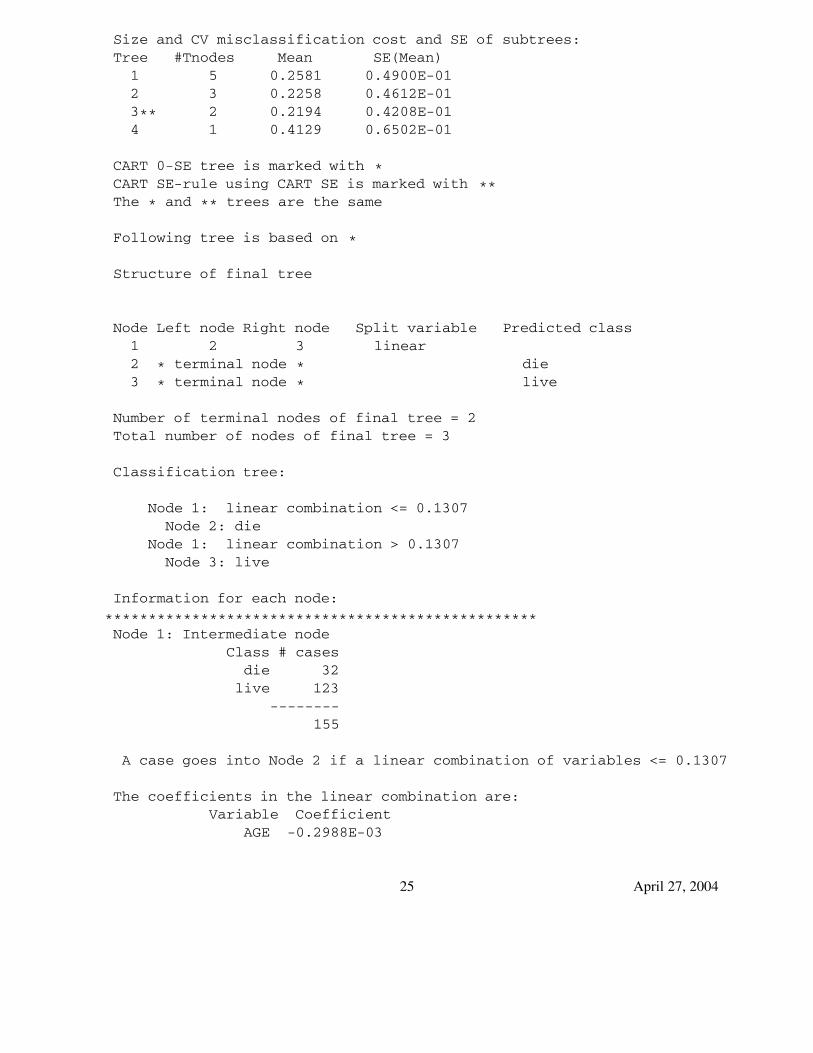
Size and CV misclassification cost and SE of subtrees:Tree #Tnodes Mean SE(Mean)

1 5 0.2581 0.4900E-012 3 0.2258 0.4612E-013** 2 0.2194 0.4208E-014 1 0.4129 0.6502E-01

CART 0-SE tree is marked with *CART SE-rule using CART SE is marked with **The * and ** trees are the same

Following tree is based on *

Structure of final tree

Node Left node Right node Split variable Predicted class1 2 3 linear2 * terminal node * die3 * terminal node * live

Number of terminal nodes of final tree = 2Total number of nodes of final tree = 3

Classification tree:

Node 1: linear combination <= 0.1307Node 2: die

Node 1: linear combination > 0.1307Node 3: live

Information for each node:

**************************************************Node 1: Intermediate node

Class # casesdie 32

live 123--------

155

A case goes into Node 2 if a linear combination of variables <= 0.1307

The coefficients in the linear combination are:Variable Coefficient

AGE -0.2988E-03

25 April 27, 2004

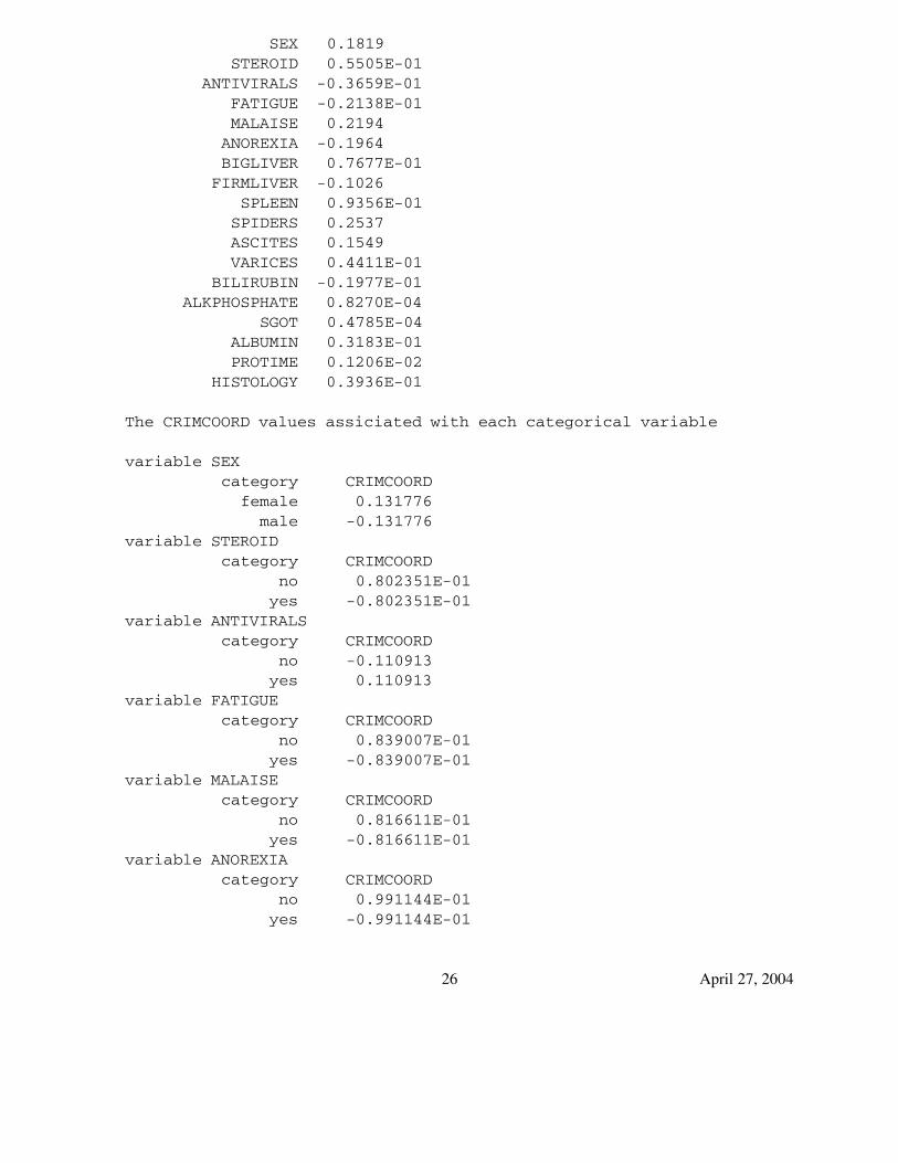
SEX 0.1819STEROID 0.5505E-01

ANTIVIRALS -0.3659E-01FATIGUE -0.2138E-01MALAISE 0.2194

ANOREXIA -0.1964BIGLIVER 0.7677E-01

FIRMLIVER -0.1026SPLEEN 0.9356E-01

SPIDERS 0.2537ASCITES 0.1549VARICES 0.4411E-01

BILIRUBIN -0.1977E-01ALKPHOSPHATE 0.8270E-04

SGOT 0.4785E-04ALBUMIN 0.3183E-01PROTIME 0.1206E-02

HISTOLOGY 0.3936E-01

The CRIMCOORD values assiciated with each categorical variable

variable SEXcategory CRIMCOORD

female 0.131776male -0.131776

variable STEROIDcategory CRIMCOORD

no 0.802351E-01yes -0.802351E-01

variable ANTIVIRALScategory CRIMCOORD

no -0.110913yes 0.110913

variable FATIGUEcategory CRIMCOORD

no 0.839007E-01yes -0.839007E-01

variable MALAISEcategory CRIMCOORD

no 0.816611E-01yes -0.816611E-01

variable ANOREXIAcategory CRIMCOORD

no 0.991144E-01yes -0.991144E-01

26 April 27, 2004

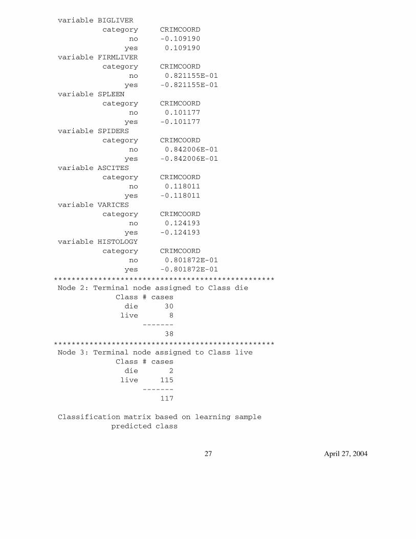
variable BIGLIVERcategory CRIMCOORD

no -0.109190yes 0.109190

variable FIRMLIVERcategory CRIMCOORD

no 0.821155E-01yes -0.821155E-01

variable SPLEENcategory CRIMCOORD

no 0.101177yes -0.101177

variable SPIDERScategory CRIMCOORD

no 0.842006E-01yes -0.842006E-01

variable ASCITEScategory CRIMCOORD

no 0.118011yes -0.118011

variable VARICEScategory CRIMCOORD

no 0.124193yes -0.124193

variable HISTOLOGYcategory CRIMCOORD

no 0.801872E-01yes -0.801872E-01

**************************************************Node 2: Terminal node assigned to Class die

Class # casesdie 30

live 8-------

38

**************************************************Node 3: Terminal node assigned to Class live

Class # casesdie 2

live 115-------

117

Classification matrix based on learning samplepredicted class

27 April 27, 2004

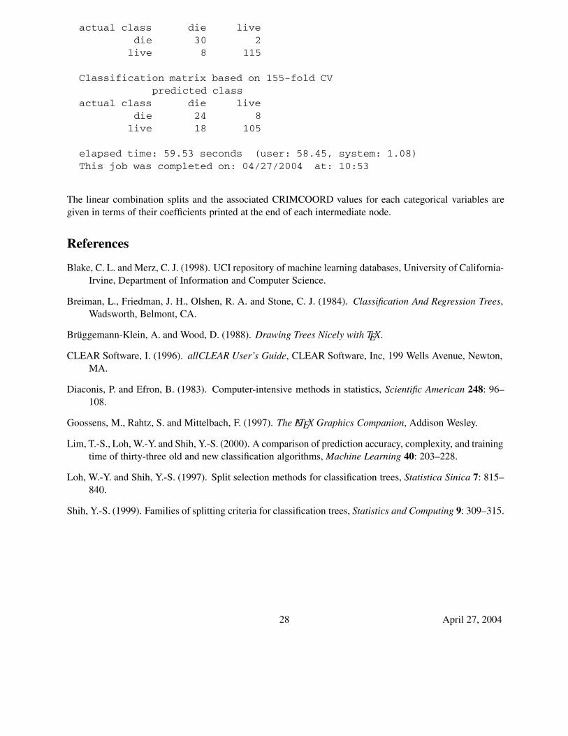
actual class die livedie 30 2

live 8 115

Classification matrix based on 155-fold CVpredicted class

actual class die livedie 24 8

live 18 105

elapsed time: 59.53 seconds (user: 58.45, system: 1.08)This job was completed on: 04/27/2004 at: 10:53

The linear combination splits and the associated CRIMCOORD values for each categorical variables aregiven in terms of their coefficients printed at the end of each intermediate node.

References

Blake, C. L. and Merz, C. J. (1998). UCI repository of machine learning databases, University of California-Irvine, Department of Information and Computer Science.

Breiman, L., Friedman, J. H., Olshen, R. A. and Stone, C. J. (1984). Classification And Regression Trees,Wadsworth, Belmont, CA.

Bruggemann-Klein, A. and Wood, D. (1988). Drawing Trees Nicely with TEX.

CLEAR Software, I. (1996). allCLEAR User’s Guide, CLEAR Software, Inc, 199 Wells Avenue, Newton,MA.

Diaconis, P. and Efron, B. (1983). Computer-intensive methods in statistics, Scientific American 248: 96–108.

Goossens, M., Rahtz, S. and Mittelbach, F. (1997). The LATEX Graphics Companion, Addison Wesley.

Lim, T.-S., Loh, W.-Y. and Shih, Y.-S. (2000). A comparison of prediction accuracy, complexity, and trainingtime of thirty-three old and new classification algorithms, Machine Learning 40: 203–228.

Loh, W.-Y. and Shih, Y.-S. (1997). Split selection methods for classification trees, Statistica Sinica 7: 815–840.

Shih, Y.-S. (1999). Families of splitting criteria for classification trees, Statistics and Computing 9: 309–315.

28 April 27, 2004