Embed Size (px)
Citation preview
University of Nebraska - LincolnDigitalCommons@University of Nebraska - LincolnComputer Science and Engineering: Theses,Dissertations, and Student Research Computer Science and Engineering, Department of
Summer 7-2017
Querying and Visualization of Moving ObjectsUsing Constraint DatabasesSemere M. WoldemariamUniversity of Nebraska - Lincoln, [email protected]
Follow this and additional works at: http://digitalcommons.unl.edu/computerscidiss
Part of the Computer Engineering Commons, Databases and Information Systems Commons,and the Numerical Analysis and Scientific Computing Commons
This Article is brought to you for free and open access by the Computer Science and Engineering, Department of at DigitalCommons@University ofNebraska - Lincoln. It has been accepted for inclusion in Computer Science and Engineering: Theses, Dissertations, and Student Research by anauthorized administrator of DigitalCommons@University of Nebraska - Lincoln.
Woldemariam, Semere M., "Querying and Visualization of Moving Objects Using Constraint Databases" (2017). Computer Science andEngineering: Theses, Dissertations, and Student Research. 133.http://digitalcommons.unl.edu/computerscidiss/133
Querying and Visualization of Moving
Objects Using Constraint Databases
by:
Semere M. Woldemariam
A THESIS
Presented to the Faculty of
The Graduate College at the University of Nebraska
In Partial Fulfillment of Requirements
For the Degree of Master of Science
Major: Computer Science
Under the Supervision of Professor Peter Revesz
Lincoln, Nebraska
July, 2017
QUERYING AND VISUALIZATION OF MOVING
OBJECTS USING CONSTRAINT DATABASES
Semere Woldemariam, M.S.
University of Nebraska, 2017
Advisor: Peter Revesz
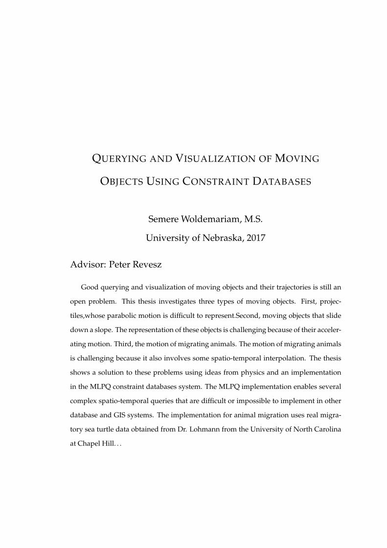
Good querying and visualization of moving objects and their trajectories is still an
open problem. This thesis investigates three types of moving objects. First, projec-
tiles,whose parabolic motion is difficult to represent.Second, moving objects that slide
down a slope. The representation of these objects is challenging because of their acceler-
ating motion. Third, the motion of migrating animals. The motion of migrating animals
is challenging because it also involves some spatio-temporal interpolation. The thesis
shows a solution to these problems using ideas from physics and an implementation
in the MLPQ constraint databases system. The MLPQ implementation enables several
complex spatio-temporal queries that are difficult or impossible to implement in other
database and GIS systems. The implementation for animal migration uses real migra-
tory sea turtle data obtained from Dr. Lohmann from the University of North Carolina
at Chapel Hill. . .

iii
Acknowledgements
First, I would like to acknowledge my advisor Dr Peter Revesz for his patient guidance.
Second, thanks to my thesis committee members Dr Lisong Xu and Dr Ashok Samal for
reviewing my work for its betterment . . .
iv
Contents
Abstract
Acknowledgements iii
1 Introduction 1
1.1 Background . . . . . . . . . . . . . . . . . . . . . . . . . . . . . . . . . . . 1
1.2 Thesis Outline . . . . . . . . . . . . . . . . . . . . . . . . . . . . . . . . . . 2
1.3 Major Thesis Contribution . . . . . . . . . . . . . . . . . . . . . . . . . . . 3
2 Constraint Database Representation of a Projectile Motion In MLPQ System 4
2.1 Background – Projectile Motion Problem . . . . . . . . . . . . . . . . . . . 4
2.1.1 Vectors . . . . . . . . . . . . . . . . . . . . . . . . . . . . . . . . . . 5
2.1.2 One Dimensional Motion . . . . . . . . . . . . . . . . . . . . . . . 6
2.2 Implementation of Constraint Database - Projectile Motion . . . . . . . . 7
2.3 Result and Analysis . . . . . . . . . . . . . . . . . . . . . . . . . . . . . . . 9
2.4 Discussion and Conclusion . . . . . . . . . . . . . . . . . . . . . . . . . . 14
3 Constraint Database Representation of Inclined Plane in MLPQ System 17
3.1 Background – Incline Plane Problem . . . . . . . . . . . . . . . . . . . . . 17
3.2 Implementation of Constraint Database - Inclined Plane . . . . . . . . . . 20
3.3 Result and Analysis . . . . . . . . . . . . . . . . . . . . . . . . . . . . . . . 21
3.4 Discussion and Conclusion . . . . . . . . . . . . . . . . . . . . . . . . . . 26
4 Constraint Database Representation of Sea Turtle in MLPQ System 27
4.1 Background . . . . . . . . . . . . . . . . . . . . . . . . . . . . . . . . . . . 27

v
4.2 Analysis of the Original Data . . . . . . . . . . . . . . . . . . . . . . . . . 28
4.3 Minimizing Data Aberration . . . . . . . . . . . . . . . . . . . . . . . . . . 32
4.4 Implementation of Constraint Database . . . . . . . . . . . . . . . . . . . 36
4.5 Result and Analysis . . . . . . . . . . . . . . . . . . . . . . . . . . . . . . . 38
4.6 Discussion and Conclusion . . . . . . . . . . . . . . . . . . . . . . . . . . 44
5 Conclusion 46

vi
List of Figures
2.1 Vector Addition . . . . . . . . . . . . . . . . . . . . . . . . . . . . . . . . . 5
2.2 Trajectory of a Projectile . . . . . . . . . . . . . . . . . . . . . . . . . . . . 7
2.3 Projectile Constraint Database Design . . . . . . . . . . . . . . . . . . . . 9
2.4 Snippets of Constraint Databases of Projectiles . . . . . . . . . . . . . . . 11
2.5 Result of Constraint Database Representation of Projectile Motion . . . . 13
2.6 Result of the Query of the Constraint Database Representation of Projec-
tile Motion . . . . . . . . . . . . . . . . . . . . . . . . . . . . . . . . . . . . 14
3.1 Diagrammatical Illustration of an Inclined Plane . . . . . . . . . . . . . . 18
3.2 Free – Body Diagram of a Sliding Object on a Frictionless Inclined Plane 19
3.3 Inclined Plane Constraint Database Design . . . . . . . . . . . . . . . . . 21
3.4 Snippet of Constraint Database of Inclined Plane . . . . . . . . . . . . . 23
3.5 Result of Constraint Database Representation of an Inclined Plane . . . . 24
3.6 Result of the Query of the Constraint Database Representation of an In-
clined Plane . . . . . . . . . . . . . . . . . . . . . . . . . . . . . . . . . . . 25
4.1 Original Data of the Sea Turtles . . . . . . . . . . . . . . . . . . . . . . . . 31
4.2 Modified Data of the Sea Turtles . . . . . . . . . . . . . . . . . . . . . . . 35
4.3 Snippet of the Constraint Database of the US Map . . . . . . . . . . . . . 36
4.4 Snippet of the Constraint Database Irving . . . . . . . . . . . . . . . . . . 37
4.5 Result of Dexter’s moving object constraint database representation . . . 38
4.6 Result of Irvings’s moving object constraint database representation . . 39
4.7 Result of Nala’s moving object constraint database representation . . . . 40
4.8 Query on the Position of Irving at a Given Time . . . . . . . . . . . . . . 41

vii
4.9 Query on the Position of All Turtles at a Given Time . . . . . . . . . . . . 42
4.10 Query on the most Eastern Turtle at a Given Time . . . . . . . . . . . . . 43

viii
Dedicated to my late father Mihreteab Woldemariam and mymother Tiblets Fitawu. . .
1
Chapter 1
Introduction
1.1 Background
It may be fair to say, moving object constraint database is not a new concept now. How-
ever, the representation of accelerating objects in a constraint database, so that to be able
to query them and be able to visualize them, still has its challenges. For example, arcGIS
and Oracle Spatial either don’t represent the motion of all continuous rigid motions of
objects or don’t represent accelerating objects. This thesis presents the representation of
some accelerating objects, based on physics concepts, and hence be able to query and
visualize them using MLPQ system.
MLPQ (Management of Linear Programming Queries) is a constraint -relational database
system that is continuously built and upgraded at the University of Nebraska - Lincoln,
since 1995 [3][4][5]. It extends the relational database by incorporating data represented
by a linear function over k attribute variables. The linear function serves as a bound
for the data by the linear inequality relation of the attributes, hence it is a constraint
database. Several query operations can be performed on the data, same way as in rela-
tional database, but enhanced as it is not limited to a finite data. Such data constrained
by the linear function constitutes a constraint database.
Constraint database may represent different kinds of data. For example, geographic
2
constraint database is concerned with the representation of objects and phenomena oc-
curring on the surface of the earth [3][4][5]. It may be considered as a database used
to represent a region, such as, countries, cities, roads, rivers, mountains, train and tele-
phone line networks, weather patterns, etc [3][4][5].
Constraint database can also represent the data for a moving object. Such database
is called a moving objects constraint database [3][4][5]. Basically, a moving object database
can be assumed as the temporal history of a geographic constraint database. Geo-
graphic constraint database and moving object constraint database inspired this thesis
to revisit old physics problems, that involve acceleration, and to have look at an actual
animal migration research from a constraint database perspective.
1.2 Thesis Outline
The physics problems revisited are the projectile motion and inclined plane problems. In
Chapter 2 the representation of the projectile motion in constraint database along with
its querying and visualization is presented. Projectile motion problem involves under-
standing the trajectory of an object under a sole influence of gravitational force, after
acquiring a certain magnitude initial velocity [2].
In Chapter 3, the thesis focuses on an inclined plane. Inclined plane problem involves
additional forces other than gravitational force. It studies the motion of an object on an
inclined plane, which is a tilted surface up on which another object can move ( or sim-
ply sit, for that matter). Here, it is investigated if constraint database would be able to
represent the trajectory of a projectile and the motion of an object on an inclined plane;
thereby to be able to query the database for information, and also visualize it.
3
In Chapter 4, constraint database representation of migrating sea turtles is presented.
Dr Lohmann ( University of North Carolina - Chapel Hill), et al, [7], are studying the
migration of sea turtles in the Atlantic ocean and their homing behavior. Some of their
data, courtesy of Dr. Lohmann, is used to try to visualize the migration of the sea tur-
tles using constraint database in MLPQ system. That helps convert a finite data to a
constraint database, representing infinite data, hence to be able to have a continuous
visualization of the migration of the sea turtles, instead of dotted data.
1.3 Major Thesis Contribution
The representation of accelerating objects in a constraint database has its challenges.
By showing the representation of accelerating objects, whose motion is well defined by
physics theory, using linear piecewise approximation, may give an insight for a future
more generic approach to the problem.
Matlab can visualize equations. However, it cannot query a set of constraint objects
in any easy way. For example the question, from section 4.5, “Find the Easternmost at
time 250 hours.” is not doable in any easy way. However as we showed in section 4.5,
that query can be implemented in the MLPQ constraint database system by two simple
extended SQL queries. Hence a contribution of this thesis is showing a simple database
approach to querying scientific moving objects data.
4
Chapter 2
Constraint Database Representation
of a Projectile Motion In MLPQ
System
Projectile motion is one of the classical physics problems. The projectile motion of an
object is well defined given certain initial parameters. These parameters are related to
each other mathematically via some physics laws. Such relationship between the pa-
rameters is the basis for generating several different exercise questions and problems in
physics textbooks. Here, the thesis looks at this physical problem, from a database per-
spective, to explore if it is possible to represent the projectile with a constraint database,
thereby be able to do database query to find information about the projectile, and also
to be able to visualize it. Hence, the objective of this chapter is to try to represent a
projectile motion using constraint database in MLPQ system, and to try to be able to
query the constraint database and visualize it.
2.1 Background – Projectile Motion Problem
A projectile is anything that is given an initial velocity and then follows a path deter-
mined entirely by the effects of gravitational acceleration (and air resistance) [1]. A
batted baseball, thrown football, a package dropped from an air plane, and a bullet
shot from a rifle are all examples of projectiles. The path followed by a projectile is
5
called its trajectory[1]. The concepts of vector and one-dimensional motion, with constant
and accelerated velocities, are important background concepts for projectile motion.
2.1.1 Vectors
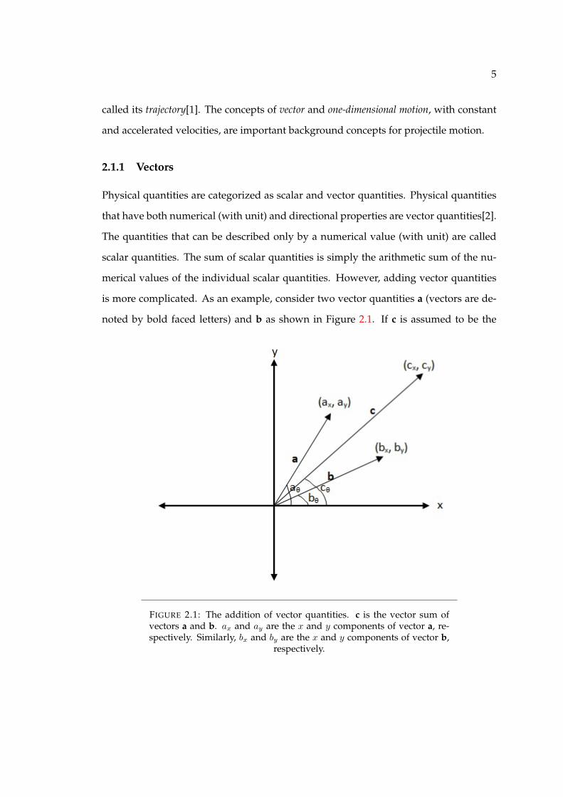
Physical quantities are categorized as scalar and vector quantities. Physical quantities
that have both numerical (with unit) and directional properties are vector quantities[2].
The quantities that can be described only by a numerical value (with unit) are called
scalar quantities. The sum of scalar quantities is simply the arithmetic sum of the nu-
merical values of the individual scalar quantities. However, adding vector quantities
is more complicated. As an example, consider two vector quantities a (vectors are de-
noted by bold faced letters) and b as shown in Figure 2.1. If c is assumed to be the
FIGURE 2.1: The addition of vector quantities. c is the vector sum ofvectors a and b. ax and ay are the x and y components of vector a, re-spectively. Similarly, bx and by are the x and y components of vector b,
respectively.
6
vector sum of vectors a and b, then the magnitude of vector c is given by,
cx = ax + bx (2.1a)
cy = ay + by (2.1b)
c =√c2x + c2y (2.1c)
The direction of the vectors a, b, and c is given in terms of the angles that the vectors
make with respect to the positive x-axis. That is,
aθ = arctan(ayax
) (2.2a)
bθ = arctan(bybx
) (2.2b)
cθ = arctan(cycx
) (2.2c)
2.1.2 One Dimensional Motion
One dimensional motion is a motion along a straight line [2]. One dimensional motion
may have a constant velocity, or it may be accelerating. If we assume the direction
of motion of an object is along the positive x-axis starting from the origin, then for a
constant velocity v motion, the position x at a time t is given by:
x = vt (2.3)
If the motion is an accelerating motion, then the position of the object is given by,
x = vot+1
2at2 (2.4)
where a is the acceleration of the object.
7
Projectile motion is the vector sum of a constant velocity horizontal motion and an
accelerated vertical motion. The horizontal motion has a velocity equal to the horizon-
tal component of the initial velocity throughout the trajectory. The vertical component
of the projectile motion is an accelerating motion. The acceleration is due to gravity,
which is approximately g = 9.8m/s2.
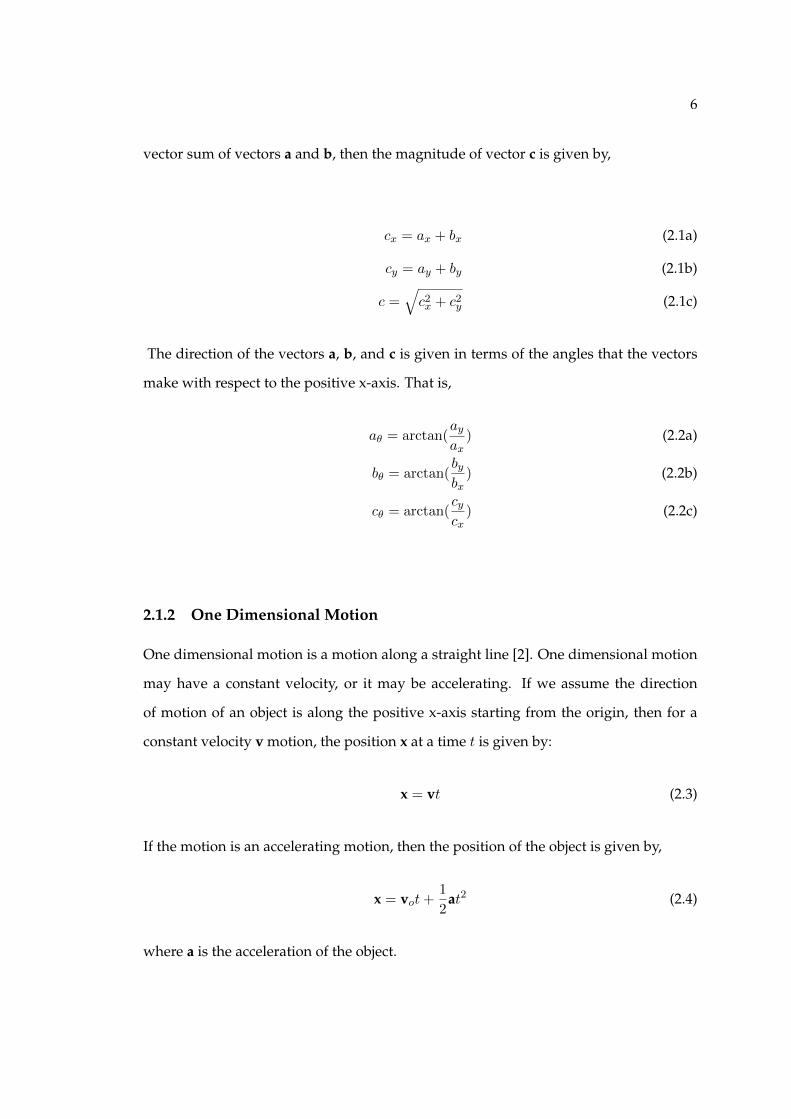
2.2 Implementation of Constraint Database - Projectile Motion
Consider the projectile trajectory in Figure 2.2
FIGURE 2.2: The trajectory of a projectile. It has an initial velocity ofmagnitude v, at an angle of θ degrees from the positive x-axis direction.
The full trajectory, from launch to landing, of a projectile is determined by the mag-
nitude and direction of the initial velocity. At all time instances, the trajectory is de-
scribed by the horizontal position x and vertical position y of the projectile. Therefore,
the x and y positions, in terms of v and θ, are the following:
x = (v cos θ)t (2.5)
y = (v sin θ)t− 1
2gt2 (2.6)
8
Total horizontal distance traveled by the projectile, before it arrives on the ground,
known as range of the projectile, r, total time, T , and maximum height, H , are some of
the special characteristics of projectiles. They are given by,
r =v2 sin 2θ
g(2.7)
T =2v sin θ
g(2.8)
H =(v sin θ)2
2g(2.9)
The MLPQ system requires the constraints to be linear inequalities [3][4][5]. In
Equations 2.5 and 2.6, x is linear in terms of the variables v and t, but they are non-
linear in terms of θ. In Equation 2.5, the variable y is linear in terms of v, but it is
non-linear in terms of θ and t. One possible way to minimize the non-linearity problem
of x and y over θ is to have different databases for different specific angles in MLPQ
system.
In Equation 2.6, it can be seen that y is not a linear function of t. But it is possible
to approximate it into a linear inequality in t, i.e., take several values of t (that span
throughout the trajectory) and their corresponding y values, then use a linear piece-wise
approximation method to get a linear function of t [6]. At this point, Equations 2.5 and
2.6 are ready to be used for the design of a database for representing a projectile motion.
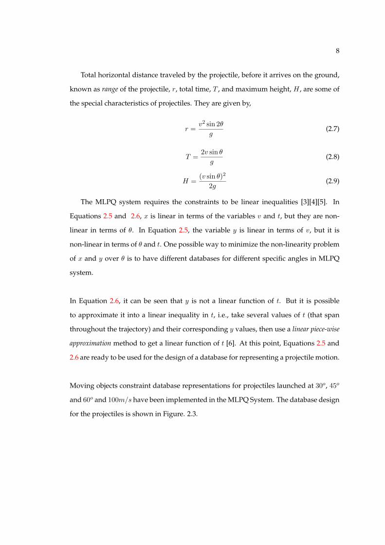
Moving objects constraint database representations for projectiles launched at 30o, 45o
and 60o and 100m/s have been implemented in the MLPQ System. The database design
for the projectiles is shown in Figure. 2.3.
9
FIGURE 2.3: Constraint database design for three projectiles and a land.The box30deg design represents the constraint database for a projectilelaunched at 30o. Similarly, the box45deg and the box60deg projectiles rep-resent for projectiles launched at 45o and 60o, respectively. Finally, land
is a constraint database for the ground level
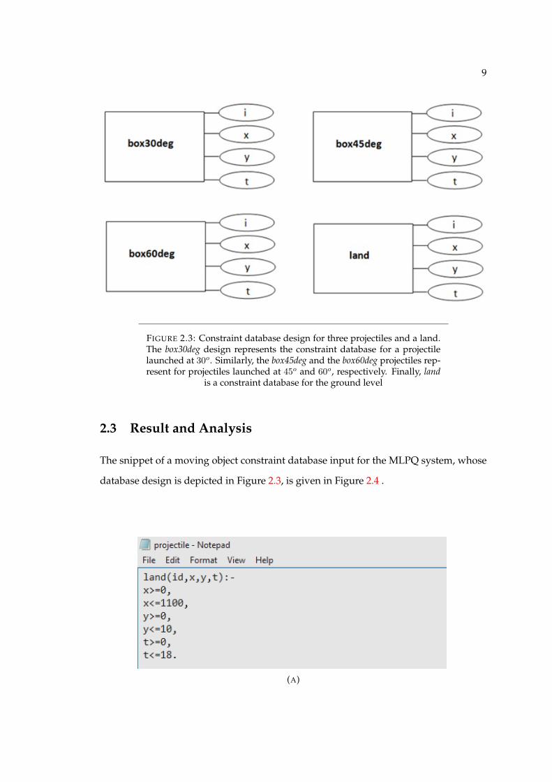
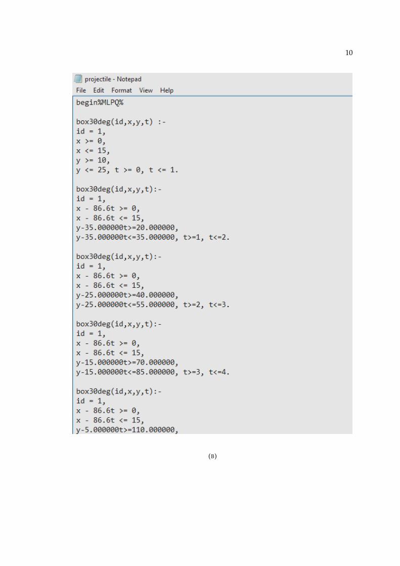
2.3 Result and Analysis
The snippet of a moving object constraint database input for the MLPQ system, whose
database design is depicted in Figure 2.3, is given in Figure 2.4 .
(A)
10
(B)
11
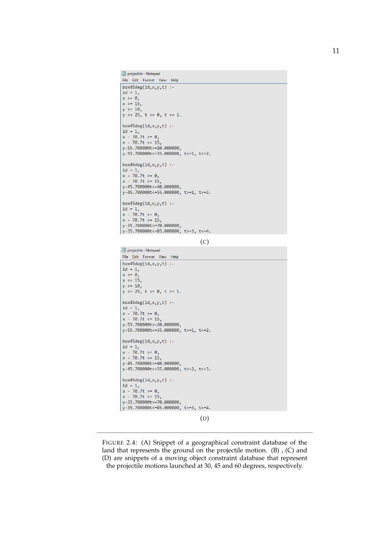
(C)
(D)
FIGURE 2.4: (A) Snippet of a geographical constraint database of theland that represents the ground on the projectile motion. (B) , (C) and(D) are snippets of a moving object constraint database that represent
the projectile motions launched at 30, 45 and 60 degrees, respectively.

12
The projectiles are represented by moving object constraint databases. Before launch,
i.e. time t = 0, the projectiles can be assumed of geographical databases represent-
ing 15 x 15 square shape, located at the origin. After launch, they are moving object
databases changing their position according to their projectile path. box30deg(i, x, y),
box45deg(i, xy) and box60deg(i, x, y) are the moving object constraint databases repre-
senting the three projectiles launched at 30 , 45 and 60 degrees, respectively.
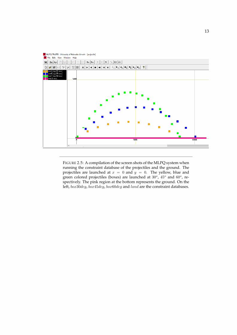
Figure 2.5 shows screen shot of the animation of the constraint database representing
the projectiles and the ground in MLPQ system. The screen shots were taken at each
step of MLPQ system animation. This means, multiple screen shots were taken, from
the launch to the landing. All the screen shots were then compiled into one picture.
Note that, all the screen shots are exactly the same except the projectiles are displaced
in every next screen shot. Hence, when compiled into one picture, it appears each pro-
jectile to have a sequence of the same box in a projectile path.
It is also interesting to note that at the time of launch, i.e. when time t = 0, there is
only one green colored box visible. During flight there are three (green, blue and yel-
low) boxes. After landing there are two boxes. There is reason related to the physics of
the projectiles and how MLPQ system runs. It is discussed under the Discussion and
Conclusion section.
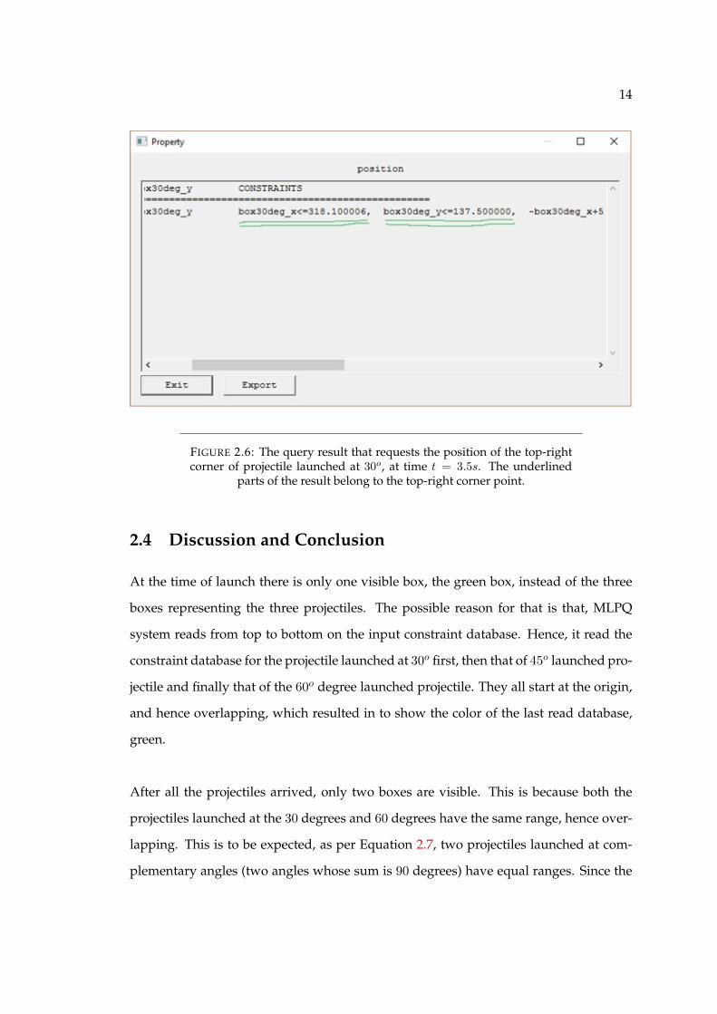
Finally, to check the accuracy of the information stored in the constraint database,
database query was made. The idea is to make a position query at a random time
and compare the query result with a mathematical result from Equations 2.5 and 2.6.
Hence, a query was made on the box30deg() constraint database, to find the position of
the top-right corner point of the projectile after 3.5s.Note that, at the time t = 0s,the po-
sition of the top-right corner point is (15, 25). Figure 2.6 shows the query result, which
is (318.100, 137.500). The result through mathematical calculation is (318.109, 139.975).
13
FIGURE 2.5: A compilation of the screen shots of the MLPQ system whenrunning the constraint database of the projectiles and the ground. Theprojectiles are launched at x = 0 and y = 0. The yellow, blue andgreen colored projectiles (boxes) are launched at 30o, 45o and 60o, re-spectively. The pink region at the bottom represents the ground. On theleft, box30deg, box45deg, box60deg and land are the constraint databases.
14
FIGURE 2.6: The query result that requests the position of the top-rightcorner of projectile launched at 30o, at time t = 3.5s. The underlined
parts of the result belong to the top-right corner point.
2.4 Discussion and Conclusion
At the time of launch there is only one visible box, the green box, instead of the three
boxes representing the three projectiles. The possible reason for that is that, MLPQ
system reads from top to bottom on the input constraint database. Hence, it read the
constraint database for the projectile launched at 30o first, then that of 45o launched pro-
jectile and finally that of the 60o degree launched projectile. They all start at the origin,
and hence overlapping, which resulted in to show the color of the last read database,
green.
After all the projectiles arrived, only two boxes are visible. This is because both the
projectiles launched at the 30 degrees and 60 degrees have the same range, hence over-
lapping. This is to be expected, as per Equation 2.7, two projectiles launched at com-
plementary angles (two angles whose sum is 90 degrees) have equal ranges. Since the
15
projectile launched at 60 degrees arrive later than the one launched at 30 degrees, the
color of the overlap box is green. Moreover, according to Equation 2.7, the maximum
range occurs at a launch angle of 45 degrees. This is consistent with the result in Fig-
ure 2.5, where the blue projectile traveled the farthest horizontally.
On arriving to the ground, the yellow (30o projectile), blue (45o projectile) and green
( 60o projectile) boxes arrived in that order. This is also consistent with Equation 2.8.
The total time of flight increases with the increase of the launching angle (sine of an
angle increases with the increase of the angle in the range [0, 90]).
Maximum height of a projectile increases proportionally with the square of the sine
of the launching angle, according to Equation 2.9. As can be seen in Figure 2.5, the
maximum height of the three projectiles, in their angle of launch, is ranked, highest to
lowest, 60o, 45o and 30o.
The accuracy of the result is not only relative to each other. For example, in calculating
the range of the projectile launched at 45o, with initial speed of 100m/s, the result is
1000m, according to Equation 2.7. In Figure 2.5, the blue box (45o projectile) arrives
1000m away from the origin.
As mentioned on the previous section, when querying the position of the projectile
launched at 30o, its top-right corner point, the query result and the mathematical re-
sults were almost equal. The slight discrepancy on the y component may be attributed
to the linear piecewise approximation performed on the y component of the position
when implementing the database (there was no linear piecewise approximation on the
x component, because it was linear). The goal of this chapter was to show that a projec-
tile motion (which is accelerated motion) can be represented by a constraint database,
using the MLPQ System. The variables of constraint databases need to be linear. Equa-
tions 2.5 and 2.6, which define the trajectory of projectile, have non-linear variables. By
16
constructing database for specific angles and by approximating the quadratic depen-
dence of position on time into a linear dependence,using linear piecewise approxima-
tion, this chapter showed that it is possible to represent projectile motion in constraint
database.

17
Chapter 3
Constraint Database Representation
of Inclined Plane in MLPQ System
Inclined plane problem is a physics problem that applies Newton’s second law[1]. As
projectile motion is a common problem in two dimensional motion problems in physics,
inclined plane problem is a common problem in the application of Newton’s second
law. There are several problems in physics textbooks that stem from the inclined plane
model, with or without friction. Here the focus is on frictionless inclined plane problem.
In projectile motion, the motion is affected only by gravity. In inclined plane problem,
however, there is additional normal force involved ( assuming frictional force is ignored,
as is the case here)[1]. The textbooks solve the problem using Newton’s second law,
that relates the net force applied to the acceleration of an object, mathematically. In
this chapter, however, it is tried to represent an inclined plane problem using constraint
database in MLPQ system.
3.1 Background – Incline Plane Problem
Any tilted surface upon which an object can slide up or down can be considered an
inclined plane. A slide at a park, interstate exit ramp, truck loading ramp are all exam-
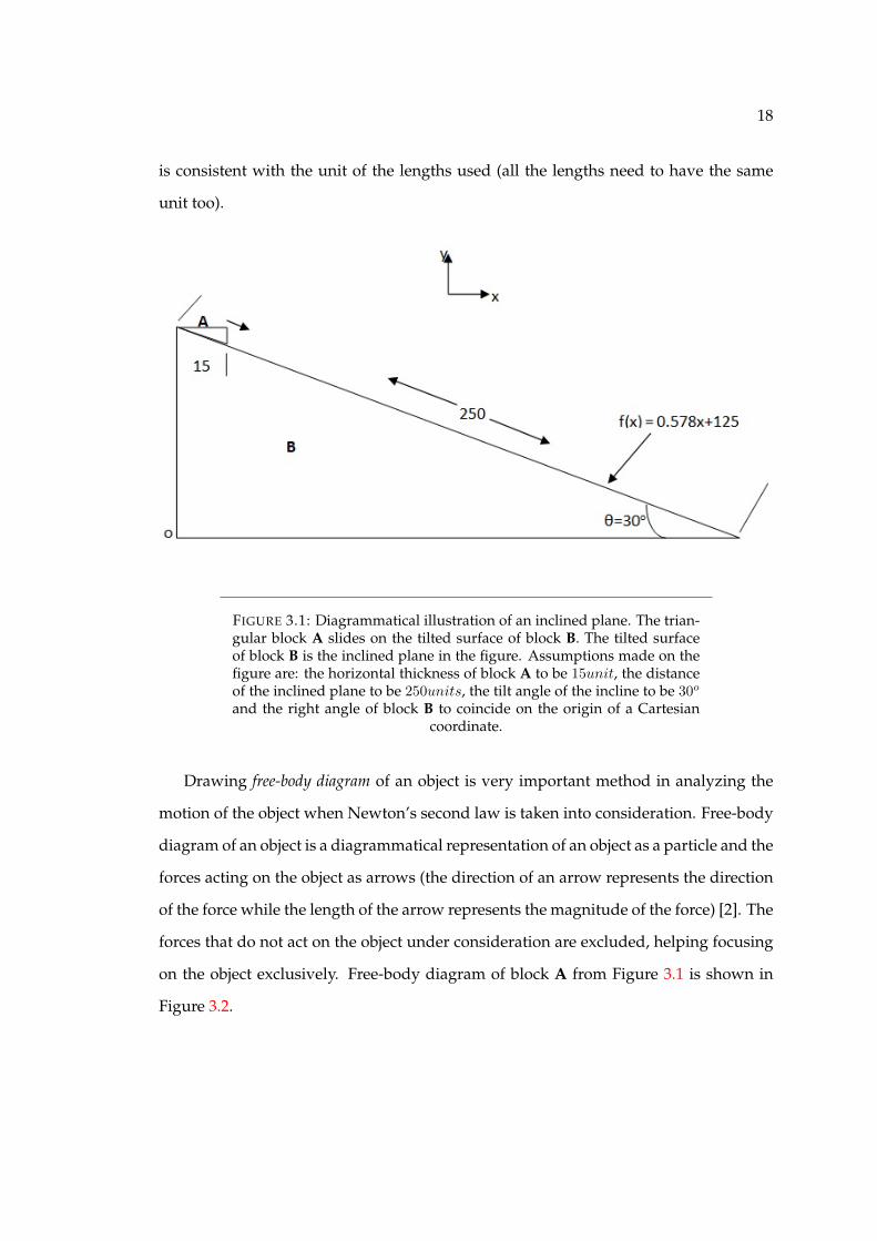
ples of inclined planes. Figure 3.1 shows a diagrammatical illustration of an inclined
plane. Note that the quantities of the lengths used are random. Moreover, the units of
the lengths do not impact the quantity of the result, as long as that the unit of the result
18
is consistent with the unit of the lengths used (all the lengths need to have the same
unit too).
FIGURE 3.1: Diagrammatical illustration of an inclined plane. The trian-gular block A slides on the tilted surface of block B. The tilted surfaceof block B is the inclined plane in the figure. Assumptions made on thefigure are: the horizontal thickness of block A to be 15unit, the distanceof the inclined plane to be 250units, the tilt angle of the incline to be 30o
and the right angle of block B to coincide on the origin of a Cartesiancoordinate.
Drawing free-body diagram of an object is very important method in analyzing the
motion of the object when Newton’s second law is taken into consideration. Free-body
diagram of an object is a diagrammatical representation of an object as a particle and the
forces acting on the object as arrows (the direction of an arrow represents the direction
of the force while the length of the arrow represents the magnitude of the force) [2]. The
forces that do not act on the object under consideration are excluded, helping focusing
on the object exclusively. Free-body diagram of block A from Figure 3.1 is shown in
Figure 3.2.
19
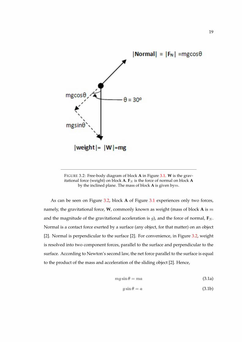
FIGURE 3.2: Free-body diagram of block A in Figure 3.1. W is the grav-itational force (weight) on block A. FN is the force of normal on block A
by the inclined plane. The mass of block A is given bym.
As can be seen on Figure 3.2, block A of Figure 3.1 experiences only two forces,
namely, the gravitational force, W, commonly known as weight (mass of block A is m
and the magnitude of the gravitational acceleration is g), and the force of normal, FN .
Normal is a contact force exerted by a surface (any object, for that matter) on an object
[2]. Normal is perpendicular to the surface [2]. For convenience, in Figure 3.2, weight
is resolved into two component forces, parallel to the surface and perpendicular to the
surface. According to Newton’s second law, the net force parallel to the surface is equal
to the product of the mass and acceleration of the sliding object [2]. Hence,
mg sin θ = ma (3.1a)
g sin θ = a (3.1b)
20
where, a is the magnitude of the acceleration of block A on the surface of the block B.
Therefore, the magnitude of the acceleration of block A on the surface of the inclined
plane (block B) is given by Equation 3.1. It is assumed to start from rest at the top of
the inclined plane accelerating down, parallel to the surface. The position of block A,
at any time t, using Equation 2.4, is then given by,
x = (1
2(g sin θ)t2) cos θ (3.2)
y = (250− 1
2(g sin θ)t2) sin θ (3.3)
Note that in both Equations 3.2 and 3.3, θ = 30o.
3.2 Implementation of Constraint Database - Inclined Plane
The goal here is to be able to represent blocks A and B in Figure 3.1, using constraint
database in MLPQ system. Since block A is a moving object, it is represented by a mov-
ing object constraint database. However, block B does not move, hence it is represented
with a geographical constraint database.
In defining the constraints for the blocks, it is important to first find the equation of
the line that represents the inclined plane. And it is given by,
y = 0.578x+ 125 (3.4)
As mentioned in the previous chapter, MLPQ system requires its constraint database
variables to be linear [3][4][5]. Therefore, Equation 3.4 is important in describing y, in
terms of a linear variable x.
21
Now it can be seen block B to be bounded in,
x ≥ 0, x ≤ 250 cos θ
y ≤ 0.578x+ 125
(3.5)
and block A is bounded by,
x ≥ T, x ≤ T + 15
y ≥ 0.578x+ 125
where T = (12(g sin 30o)t2) cos 30o
(3.6)
In Equation 3.6, T is not linear in t. Therefore, linear piecewise approximation is used to
convert it into linear inequality [6].
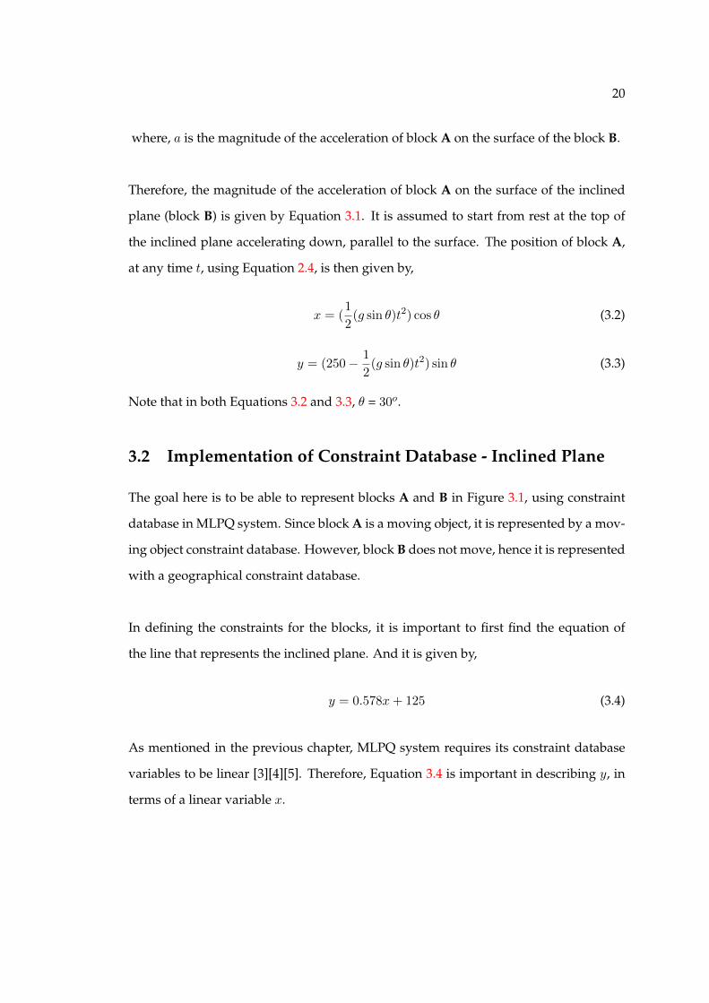
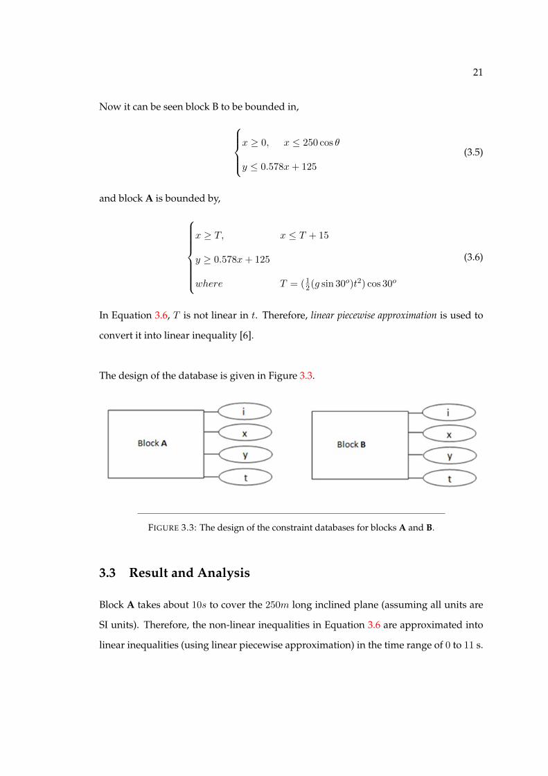
The design of the database is given in Figure 3.3.
FIGURE 3.3: The design of the constraint databases for blocks A and B.
3.3 Result and Analysis
Block A takes about 10s to cover the 250m long inclined plane (assuming all units are
SI units). Therefore, the non-linear inequalities in Equation 3.6 are approximated into
linear inequalities (using linear piecewise approximation) in the time range of 0 to 11 s.

22
The snippet of the input of constraint database in MLPQ system for the blocks is shown
in Figure 3.4.

23
FIGURE 3.4: Constraint database input of MLPQ system for blocksA and B. incline(id, x, y, t) is the constraint database for block B and
slideBox(id, x, y, t) is constraint database for block A.
24
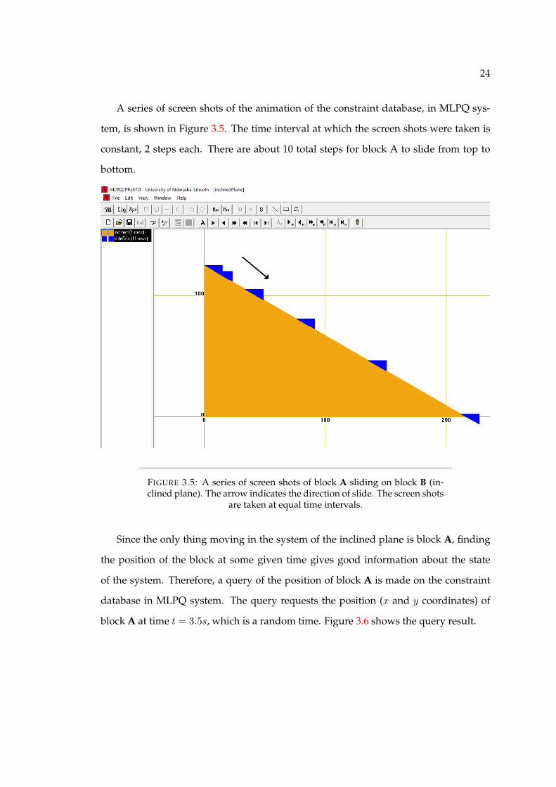
A series of screen shots of the animation of the constraint database, in MLPQ sys-
tem, is shown in Figure 3.5. The time interval at which the screen shots were taken is
constant, 2 steps each. There are about 10 total steps for block A to slide from top to
bottom.
FIGURE 3.5: A series of screen shots of block A sliding on block B (in-clined plane). The arrow indicates the direction of slide. The screen shots
are taken at equal time intervals.
Since the only thing moving in the system of the inclined plane is block A, finding
the position of the block at some given time gives good information about the state
of the system. Therefore, a query of the position of block A is made on the constraint
database in MLPQ system. The query requests the position (x and y coordinates) of
block A at time t = 3.5s, which is a random time. Figure 3.6 shows the query result.
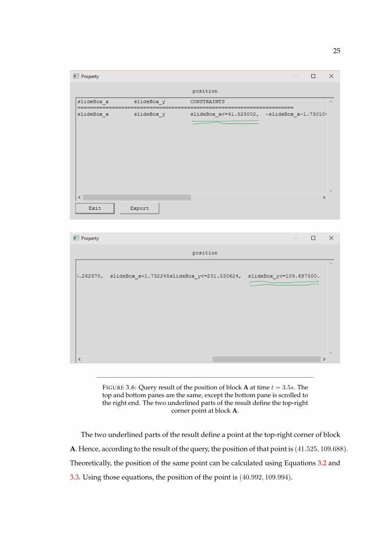
25
FIGURE 3.6: Query result of the position of block A at time t = 3.5s. Thetop and bottom panes are the same, except the bottom pane is scrolled tothe right end. The two underlined parts of the result define the top-right
corner point at block A.
The two underlined parts of the result define a point at the top-right corner of block
A. Hence, according to the result of the query, the position of that point is (41.525, 109.688).
Theoretically, the position of the same point can be calculated using Equations 3.2 and
3.3. Using those equations, the position of the point is (40.992, 109.994).
26
3.4 Discussion and Conclusion
In Figure 3.5, the screen shots are taken at equal time interval, 2 steps each (in SI unit a
step may represent 1 second). However, it is important to note that the distance covered
in between each screen shot is not equal. It increases in each successive interval. This
has physical significance. It implies that the block was accelerating when it was sliding
down.
From Figure 3.5 it is possible to learn that the block accelerates when sliding down.
However, it is not easy to guess where block A is going to be after a certain time.
Therefore, accuracy of query result on the constraint database is important. Hence,
comparison of the result of a query of a position of block A (a specific reference point at
the block) with the position of the same point obtained using Equations 3.2 and 3.3 is
made. As mentioned in the previous section, the result of query and calculation of the
position of the top-right corner of block A are (41.525, 109.688) and (40.992, 109.994),
respectively. The results are very close. The slight difference may be attributed to the
approximation of non-linear inequalities to linear inequalities, using piecewise linear
approximation.
The goal of this chapter was to show the possibility of representing a frictionless in-
clined plane problem (which is an accelerated motion), using constraint database in
MLPQ system. The equations of the position of a sliding object are not linear in time
(because of acceleration), as can be seen in Equations 3.2 and 3.3. However, it is possible
to circumvent this challenge by approximating the equations using linear piecewise ap-
proximation method. Therefore, it is possible to represent a frictionless inclined plane,
at a specified angle, on a constraint database in MLPQ system.
27
Chapter 4
Constraint Database Representation
of Sea Turtle in MLPQ System
Dr. Kenneth Lohmann, et al., worked on tracing the migration of loggerhead and green
turtles [7]. The study area is in North Carolina, USA. However, the turtles migrate deep
into the Atlantic ocean. The visualization of turtle migration using constraint database
in MLPQ system, presented under this chapter, is based on the data obtained by Dr.
Kenneth Lohmann, et al [7].
4.1 Background
Animal migration is one of the most observed phenomenon in biology, probably, in no
small part, because movement itself is a defining characteristic of animals [7]. In his
book, Archie Carr, professor of zoology at the University of Florida, first published in
1956 and titled The Windward Road, mentions an incident regarding sea turtles told to
him by a captain of turtle fishermen’s boat in Cayman Islands. According to the captain,
a boat filled with sea turtles captured in their feeding area around northern Nicaragua,
was shipped to Florida. Around the coast of Florida the boat capsized. The turtles were
marked, customarily with the fishermen’s initials, and to the surprise of the fishermen
the turtles got back to where they were captured initially [8].
Dr. Lohmann, et al, have been interested on the migration of juvenile loggerhead
28
(Caretta caretta) and green (chelonia mydas) sea turtles [9]. These juvenile turtles orig-
inate from the east coast of the USA [9]. They show strong homing behavior, i.e., they
return back to their feeding sites after migration [9]. They have also studied hatchling
turtles.
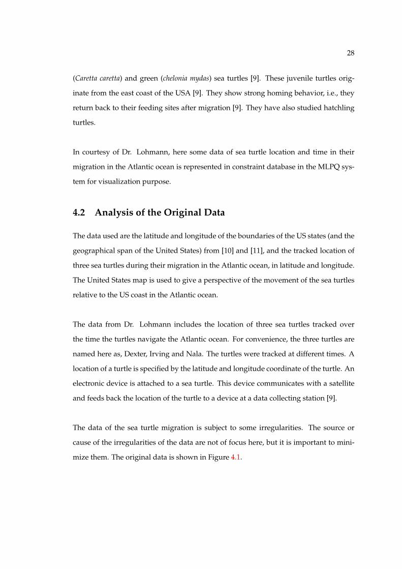
In courtesy of Dr. Lohmann, here some data of sea turtle location and time in their
migration in the Atlantic ocean is represented in constraint database in the MLPQ sys-
tem for visualization purpose.
4.2 Analysis of the Original Data
The data used are the latitude and longitude of the boundaries of the US states (and the
geographical span of the United States) from [10] and [11], and the tracked location of
three sea turtles during their migration in the Atlantic ocean, in latitude and longitude.
The United States map is used to give a perspective of the movement of the sea turtles
relative to the US coast in the Atlantic ocean.
The data from Dr. Lohmann includes the location of three sea turtles tracked over
the time the turtles navigate the Atlantic ocean. For convenience, the three turtles are
named here as, Dexter, Irving and Nala. The turtles were tracked at different times. A
location of a turtle is specified by the latitude and longitude coordinate of the turtle. An
electronic device is attached to a sea turtle. This device communicates with a satellite
and feeds back the location of the turtle to a device at a data collecting station [9].
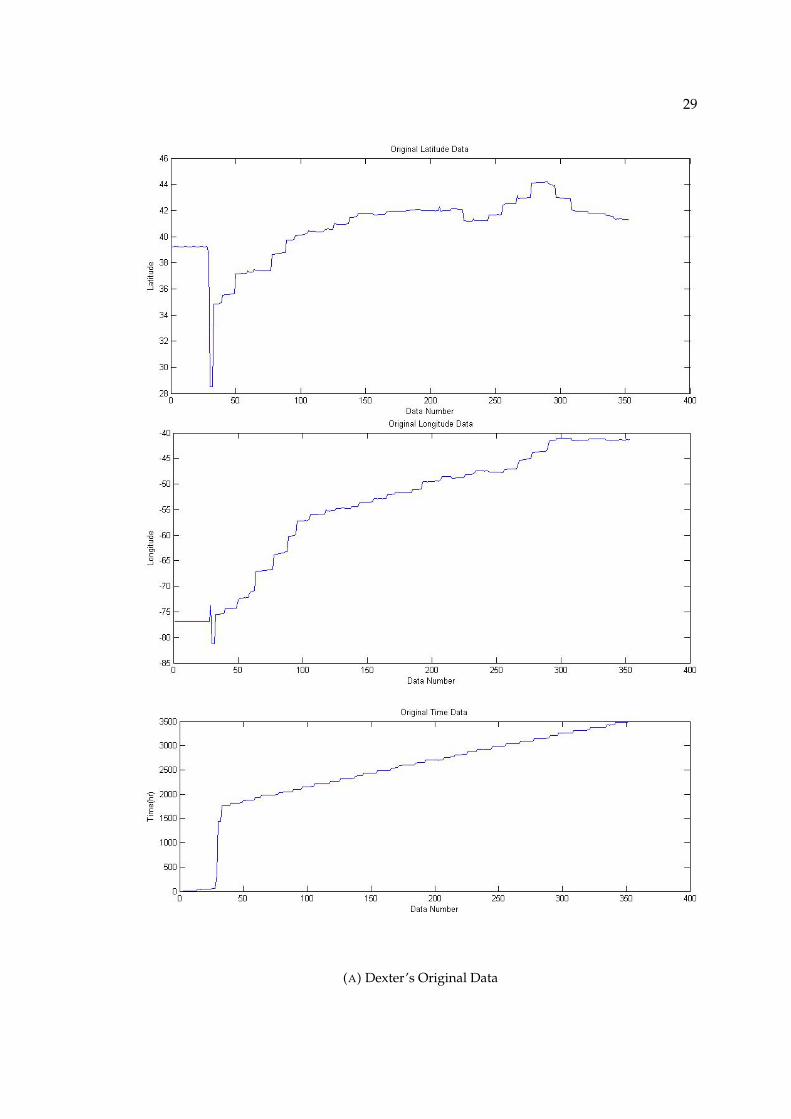
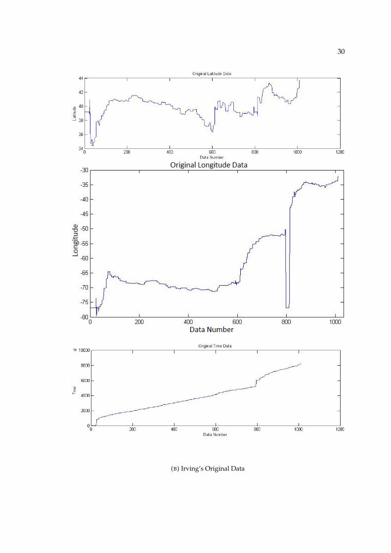
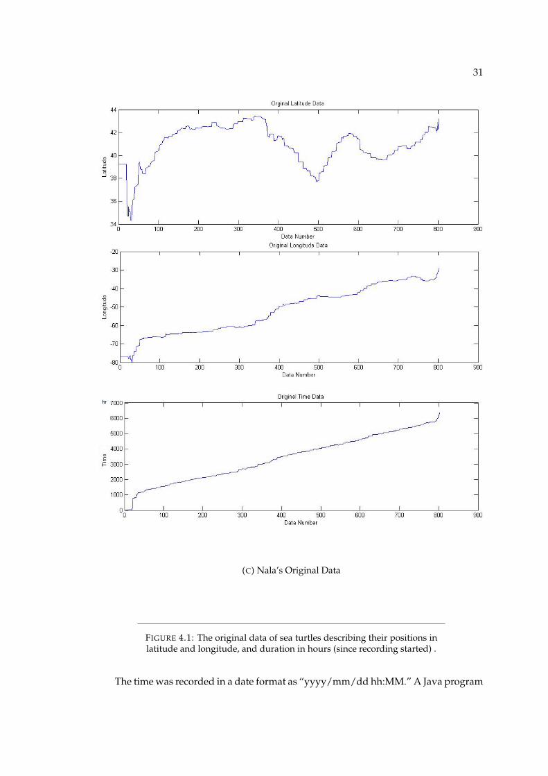
The data of the sea turtle migration is subject to some irregularities. The source or
cause of the irregularities of the data are not of focus here, but it is important to mini-
mize them. The original data is shown in Figure 4.1.
29
(A) Dexter’s Original Data
30
(B) Irving’s Original Data
31
(C) Nala’s Original Data
FIGURE 4.1: The original data of sea turtles describing their positions inlatitude and longitude, and duration in hours (since recording started) .
The time was recorded in a date format as “yyyy/mm/dd hh:MM.” A Java program
32
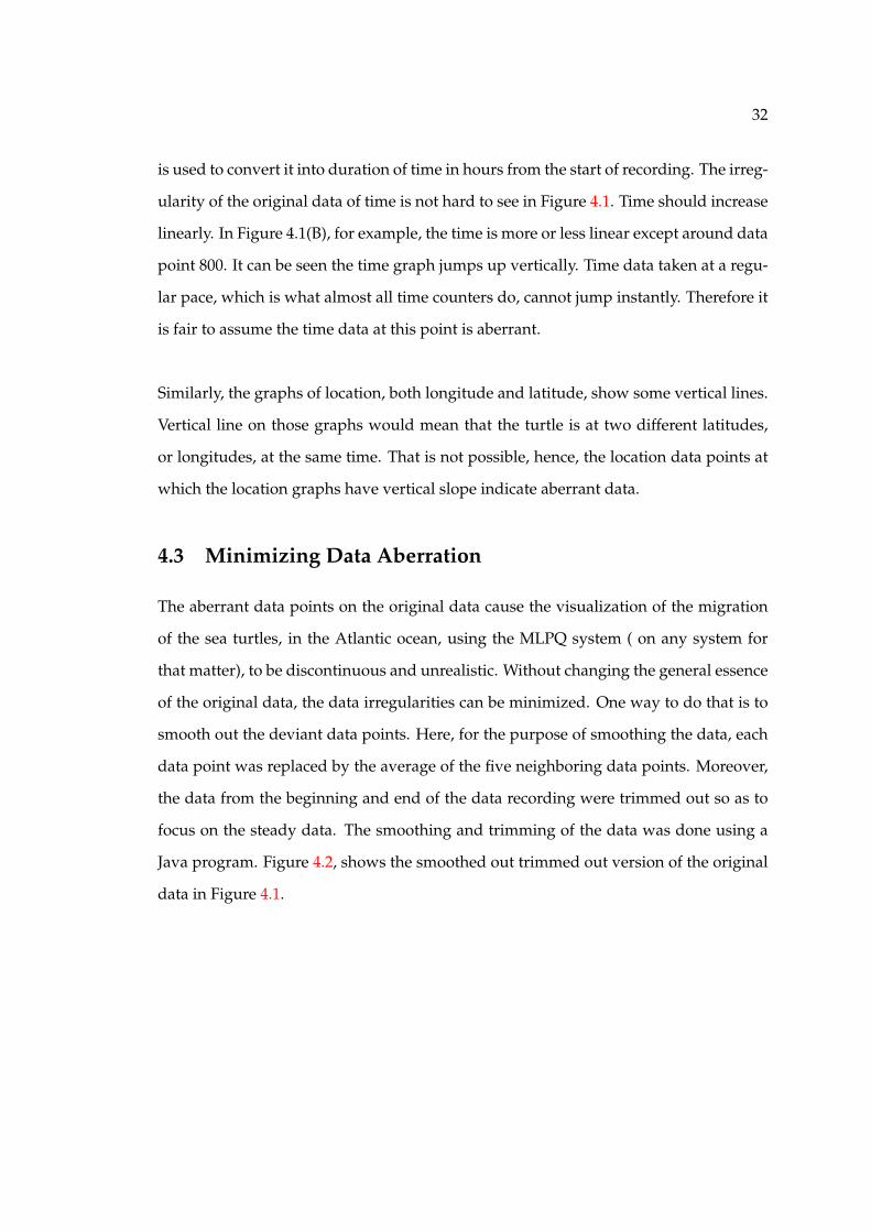
is used to convert it into duration of time in hours from the start of recording. The irreg-
ularity of the original data of time is not hard to see in Figure 4.1. Time should increase
linearly. In Figure 4.1(B), for example, the time is more or less linear except around data
point 800. It can be seen the time graph jumps up vertically. Time data taken at a regu-
lar pace, which is what almost all time counters do, cannot jump instantly. Therefore it
is fair to assume the time data at this point is aberrant.
Similarly, the graphs of location, both longitude and latitude, show some vertical lines.
Vertical line on those graphs would mean that the turtle is at two different latitudes,
or longitudes, at the same time. That is not possible, hence, the location data points at
which the location graphs have vertical slope indicate aberrant data.
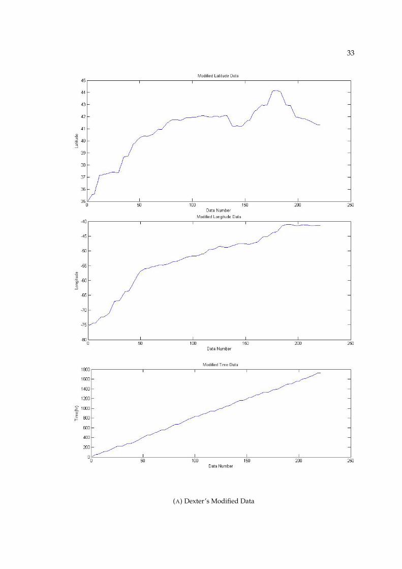
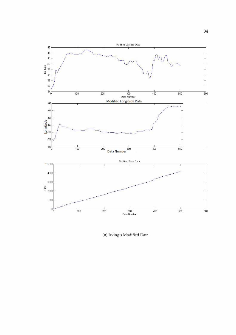
4.3 Minimizing Data Aberration
The aberrant data points on the original data cause the visualization of the migration
of the sea turtles, in the Atlantic ocean, using the MLPQ system ( on any system for
that matter), to be discontinuous and unrealistic. Without changing the general essence
of the original data, the data irregularities can be minimized. One way to do that is to
smooth out the deviant data points. Here, for the purpose of smoothing the data, each
data point was replaced by the average of the five neighboring data points. Moreover,
the data from the beginning and end of the data recording were trimmed out so as to
focus on the steady data. The smoothing and trimming of the data was done using a
Java program. Figure 4.2, shows the smoothed out trimmed out version of the original
data in Figure 4.1.
33
(A) Dexter’s Modified Data
34
(B) Irving’s Modified Data

35
(C) Nala’s Modified Data
FIGURE 4.2: The modified data of sea turtles describing their positionsin latitude and longitude, and duration in hours (since recording started)
.
36
4.4 Implementation of Constraint Database
At this point, the data is raw data with its irregularities minimized. However, in order
to be able to visualize the sea turtles movement through the Atlantic ocean, using the
MLPQ system, it is necessary to represent the data in the form of constraint database.
As afore mentioned, the constraint equations must be linear.
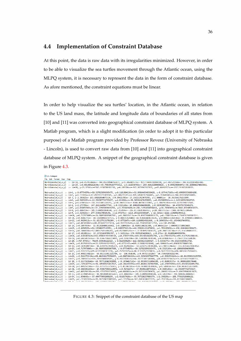
In order to help visualize the sea turtles’ location, in the Atlantic ocean, in relation
to the US land mass, the latitude and longitude data of boundaries of all states from
[10] and [11] was converted into geographical constraint database of MLPQ system. A
Matlab program, which is a slight modification (in order to adopt it to this particular
purpose) of a Matlab program provided by Professor Revesz (University of Nebraska
- Lincoln), is used to convert raw data from [10] and [11] into geographical constraint
database of MLPQ system. A snippet of the geographical constraint database is given
in Figure 4.3.
FIGURE 4.3: Snippet of the constraint database of the US map

37
As afore mentioned, the location of a sea turtle at a time is defined by its longitude
and latitude. This means the location of the sea turtle changes as either (or both) the
longitude and latitude change. Therefore, the constraint database is represented by the
linear variation of the latitude in time and the linear variation of longitude in time.
Because there is large quantity of data points, Java program is prepared to convert the
large data into a constraint database of MLPQ system for each sea turtle. A snippet of
the large MLPQ’s constraint database for Irving is given in Figure 4.4.
FIGURE 4.4: Snippet of the moving object constraint database of the Irv-ing

38
4.5 Result and Analysis
Once the constraint database for MLPQ system is prepared, running it in MLPQ is what
ensues in order to visualize the movement of the sea turtles in the Atlantic ocean. There
is the US map where each state is delineated using latitude and longitude. A sea turtle
is represented by square box which is out of scale.
Figure 4.5 is the series screen shots of running Dexter’s moving object and US’ geo-
graphical databases on MLPQ system. The screen shots were taken at about 10 steps,
in a fairly constant manner. That means the denser the boxes are the more time Dexter
took there. The arrows also indicate the direction of motion of Dexter.
FIGURE 4.5: A series of screen shots of a running MLPQ system with US’geographical constraint database and Dexter’s moving object constraint
database.
Figure 4.6 also shows, like Figure 4.5, the series of screen shots of MLPQ system
running the geographical and a moving object constraint databases for Irving. Each box
represents the position of Irving in the Atlantic ocean in about 15 steps in the MLPQ

39
system. The density of the of the boxes represents the speed, inversely, and the arrows
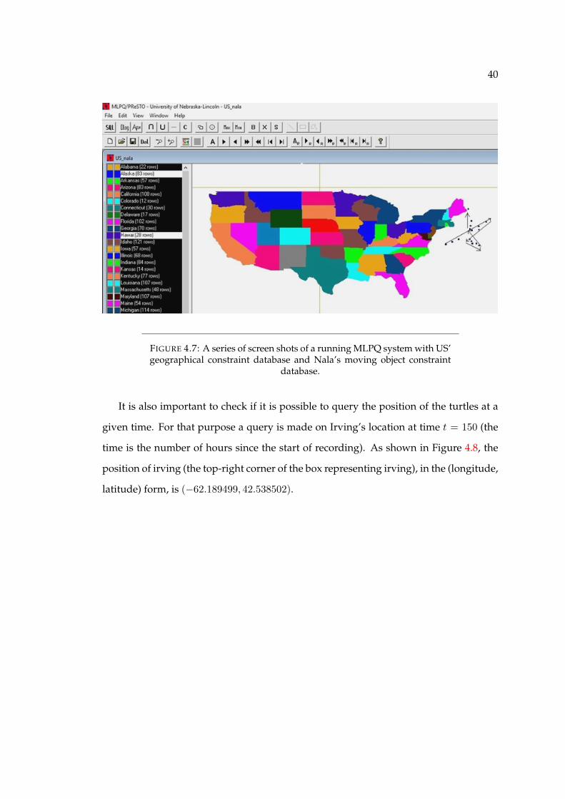
represent the direction of Irving. Finally, Figure 4.7 is like Figure 4.5 and Figure 4.6 with
the sea turtle being Nala. The shots were taken at about 15 steps of MLPQ system. Since
each step is fairly equal, the box density indicate how fast Nala was moving, while the
direction is pointed by the arrows.
FIGURE 4.6: A series of screen shots of a running MLPQ system with US’geographical constraint database and Irving’s moving object constraint
database.
40
FIGURE 4.7: A series of screen shots of a running MLPQ system with US’geographical constraint database and Nala’s moving object constraint
database.
It is also important to check if it is possible to query the position of the turtles at a
given time. For that purpose a query is made on Irving’s location at time t = 150 (the
time is the number of hours since the start of recording). As shown in Figure 4.8, the
position of irving (the top-right corner of the box representing irving), in the (longitude,
latitude) form, is (−62.189499, 42.538502).

41
(A) Query of irving’s position at time t = 150
(B) The result query of irving’s position at time t = 150
FIGURE 4.8: The query and its result of irving’s position at time t = 150.The underlined part indicates the position of the top-right corner of the
box that represents irving.
42
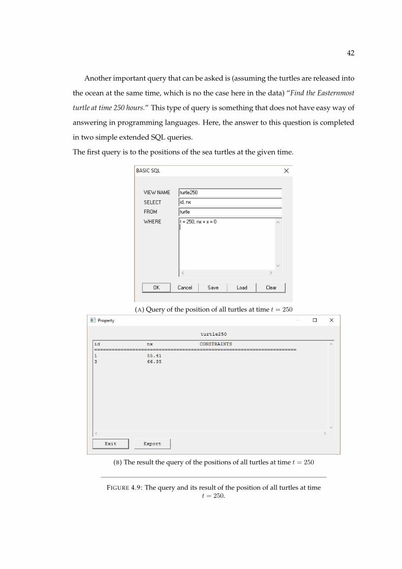
Another important query that can be asked is (assuming the turtles are released into
the ocean at the same time, which is no the case here in the data) “Find the Easternmost
turtle at time 250 hours.” This type of query is something that does not have easy way of
answering in programming languages. Here, the answer to this question is completed
in two simple extended SQL queries.
The first query is to the positions of the sea turtles at the given time.
(A) Query of the position of all turtles at time t = 250
(B) The result the query of the positions of all turtles at time t = 250
FIGURE 4.9: The query and its result of the position of all turtles at timet = 250.
43
x in the constraint database denotes the longitude of the turtles. nx and nx+ x = 0
are used to maintain positive values.The id denotes the identification number of the
turtles on the database (1 = Irving, 2 = Dexter and 3 = Nala).
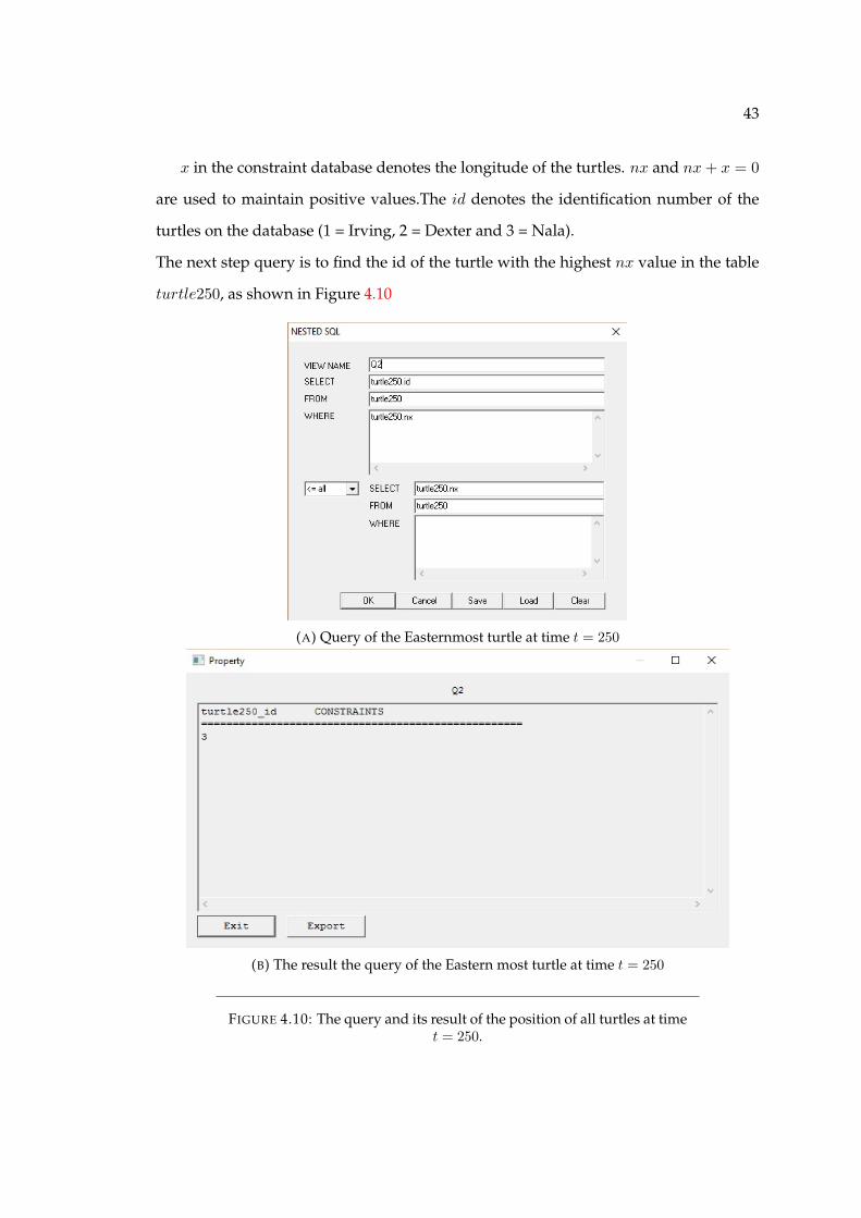
The next step query is to find the id of the turtle with the highest nx value in the table
turtle250, as shown in Figure 4.10
(A) Query of the Easternmost turtle at time t = 250
(B) The result the query of the Eastern most turtle at time t = 250
FIGURE 4.10: The query and its result of the position of all turtles at timet = 250.
44
The result is 3 which means Nala is the Easternmost with respect to the rest of the
sea turtles.
4.6 Discussion and Conclusion
The data collection of the location of Dexter seems to start when the sea turtle was at
the coast of North Carolina. After spending some time in the Atlantic ocean, it seems
to head back to the North Carolina coast. Irving started from the coast of the North
Carolina. It swam in a relatively wide area in the Atlantic ocean. The recording of
its location ends when it gets near the coast of Rhode Island. Nala also was recorded
near North Carolina coast and the recording ended near Maine. Dexter’s migration
shown by the MLPQ system seems to be consistent with the hypothesis that the sea
turtles would return to their original place after migrating deep in the Atlantic ocean.
Irvin and Nala, even though, they seem to return to a different US state, in the MLPQ
system, it is important at this point to remember that the data used was trimmed at its
beginning and its ending of the recording during the irregularity minimization process.
So there is still a possibility that the turtles have returned to the same state. Moreover,
in relation to the spread of the distance they travelled in the Atlantic ocean, the distance
between the origin and the destination is not too far.
When running the geographical constraint database and the moving object database
of the three sea turtles in the MLPQ system, there exist some random movements of the
boxes which seem to be out of sync from what would be normally expected the box to
move to. Moreover, at times, there exist double boxes for one turtle at one time. It is
fair to assume that these drawbacks originate from the data itself rather than from the
constraint database. The reason for that assumption is that, first, when a simulated data
is converted into a moving object constraint database and is run in the system, there is
no experience of abnormal movement. This is shown with simulation of a projectile
motion and an inclined plane. The second reason is understood by analyzing the given
45
data of the location of the sea turtles. Looking at Figure 4.1, it can be seen that there are
vertical lines on the graphs of the latitude and longitude. Vertical lines on these graphs
mean that the sea turtles are existing at different latitude or longitude at the same time.
To minimize such data aberration, averaging of neighbor data points was done. Even
though, this method helps minimize such data aberration, it can’t be expected to solve
the problem completely.
Finally, query of the position of irving at time t = 150 was made. The result of the
query , (−62.189499, 42.538502), is with in the Atlantic ocean, somewhere near the US
coast(around Maine), which gives more confidence on the accuracy of the constraint
database.
46
Chapter 5
Conclusion
A projectile motion constraint database was constructed using existing mathematical
relations, as in Equations 2.5 and 2.6, on MLPQ system. In the constraint database, the
trajectory of projectiles launched at 30o, 45o and 60o were represented. In investigating
the results obtained by constraint database, the projectiles’ relative total time of flight,
range and maximum height were in agreement with the theoretical expectation. More-
over, in order to test the absolute accuracy of the database, not relative to each other,
the position of the projectile at random time was queried and the result was compared
with its theoretical counterpart. A constraint database representing the motion of an
object on an inclined plane, tilted at 30o and frictionless, was also constructed, using
Equations 3.2 and 3.3, in MLPQ system. The accuracy of the database is substantiated
by looking the total time the object on the inclined plane took to slide all the way on
the inclined plane and by querying the its position at a random time. Both were com-
pared with what would be expected theoretically. Both the projectile motion and the
inclined plane problem are accelerated motions, and both were represented in a con-
straint database in this thesis.
Data obtained from a research that investigates the homing behavior of sea turtles
(courtesy of Dr. Lohmann [7]), was also used to convert it into constraint database, in
MLPQ system. The finite data, that represents the position, in latitude and longitude,
of the sea turtles at certain date, was converted into constraint database. Converting a
47
finite data into constraint database in MLPQ system can provide a continuous motion
animation in MLPQ system. Continuous motion animation gives a better perspective
in viewing the migration of the sea turtles, instead of dotted data points on a map, and
hence help make better analysis of the research results. The position data of the sea
turtles, which is in the Atlantic ocean, is better understood with the map of the United
States as reference. For this purpose, the latitude and longitude of the boundaries of all
the states was used to create a geographical constraint database of the US map. A query
on the position of one of the sea turtles was also done to show that an information can
be queried from the constraint database.
Finally, on this thesis it was shown that some accelerated motion and complicated mi-
gration movement of sea turtles could be represented on a constraint database, which
thereby can be queried and visualized. This may give an insight for a more generic
approach to representing accelerated motion in constraint database.
48
Reference
1. Young, Hugh D., Roger A. Freedman, and A. Lewis Ford. University physics with
modern physics. 11th ed. Harlow, Essex: Pearson, 2004. Print.
2. Serway, Raymond A., and John W. Jewett. Physics for scientists and engineers. Pa-
cific Grove, CA: Brooks/Cole, n.d. Print.
3. Revesz, Peter. Introduction to Databases from Biological to Spatio-Temporal. N.p.: n.p.,
n.d. Print.
4. P. C. Kanellakis, G. M. Kuper, and P. Z. Revesz, Constraint Query Languages, Journal
of Computer and System Sciences, Vol. 51, No. 1, 1995, pp.26-52.
5. P. Z. Revesz, R Chen, P. Kanjamala, Y. Li, Y. Liu, and Y. Wang, The MLPQ/GIS
Constraint Database Systems, Proceedings of the ACM-SIGMOD International Con-
ference on Management of Data, ACM Press, 2000, pp. 601
6. Burden, Richard L., and J. Douglas Faires. Numerical Analysis. 9th ed. Boston,
MA: Brooks/Cole, 2011. Print.
7. Milner-Gulland, E. J., John M. Fryxell, and Anthony R. E. Sinclair. Animal Migra-
tion: A Synthesis. Oxford: Oxford UP, 2011. Print.
8. Carr, Archie. The Windward Road: Adventures of a Naturalist on Remote Caribbean
Shores. Gainesville: U of Florida, 2013. Print.
9. Avens, L. and K. J. Lohmann. 2004. Navigation and seasonal migratory orienta-
tion in juvenile sea turtles. Journal of Experimental Biology 207: 1771-1778.
10. William, M. (n.d.). States. Retrieved from http://econym.org.uk/gmap/states.xml

49
11. Zwiefelhofer, D. B. (n.d.). Find Latitude and Longitude. Retrieved June 1, 2017,
from http://www.findlatitudeandlongitude.com/