Embed Size (px)
DESCRIPTION
Query Optimization. Why Optimize?. Given a query of size n and a database of size m , how big can the output of applying the query to the database be? Example: R(A) with 2 rows. One row has value 0. One row has value 1. How many rows are in R x R? How many in R x R x R? - PowerPoint PPT Presentation
Citation preview

1
Query OptimizationQuery Optimization

2
Why Optimize?Why Optimize?
• Given a query of size n and a database of
size m, how big can the output of applying
the query to the database be?
• Example: R(A) with 2 rows. One row has
value 0. One row has value 1.
– How many rows are in R x R?
– How many in R x R x R?
Size of output as a function of input: O( ? )
3
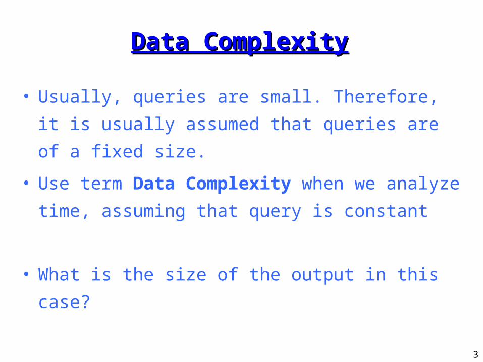
Data ComplexityData Complexity
• Usually, queries are small. Therefore, it is
usually assumed that queries are of a fixed
size.
• Use term Data Complexity when we
analyze time, assuming that query is
constant
• What is the size of the output in this case?

4
Optimizer ArchitectureOptimizer Architecture
Algebraic Space
Method-StructureSpace
Cost Model
Size-DistributionEstimator
Planner
Rewriter
5
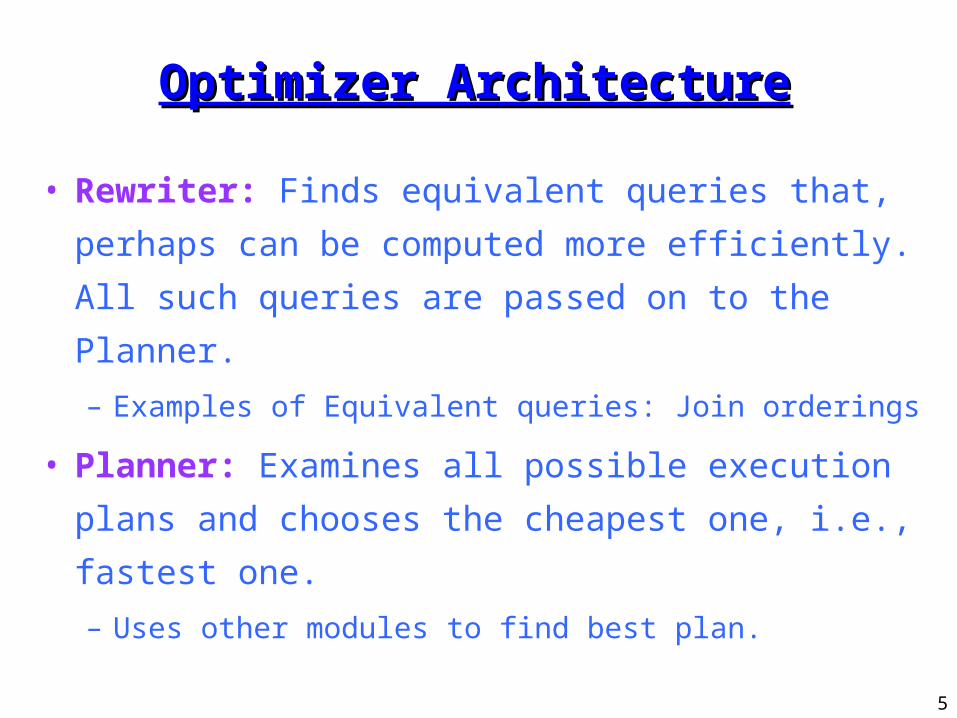
Optimizer ArchitectureOptimizer Architecture
• Rewriter: Finds equivalent queries that,
perhaps can be computed more efficiently. All
such queries are passed on to the Planner.
– Examples of Equivalent queries: Join orderings
• Planner: Examines all possible execution
plans and chooses the cheapest one, i.e.,
fastest one.
– Uses other modules to find best plan.

6
Optimizer Architecture Optimizer Architecture (cont.)(cont.)
• Algebraic Space: Determines which types of
queries will be examined.
– Example: Try to avoid Cartesian Products
• Method-Space Structure: Determines what
types of indexes are available and what types
of algorithms for algebraic operations can be
used.
– Example: Which types of join algorithms can be
used

7
Optimizer Architecture Optimizer Architecture (cont.)(cont.)
• Cost Model: Estimates the cost of
execution plans.
– Uses Size-Distribution Estimator for this.
• Size-Distribution Estimator:
Estimates size of tables, intermediate
results, frequency distribution of
attributes and size of indexes.

8
Algebraic SpaceAlgebraic Space
• We consider queries that consist of select, project and join.
(Cartesian product is a special case of join.)
• Such queries can be represented by a tree.
• Example: emp(name, age, sal, dno)
dept(dno, dname, floor, mgr, ano)
act(ano, type, balance, bno)
bank(bno, bname, address)
select name, floor
from emp, dept
where emp.dno=dept.dno and sal>100K

9
3 Trees3 Trees
name, floor
dno=dno
sal>100K
EMP
DEPT
name, floor
dno=dno
sal>100K
EMP DEPT
name, floor
dno=dno
sal>100K
EMP
DEPT
dno, floor
name,sal,dno
dno, name
T1 T2 T3
10
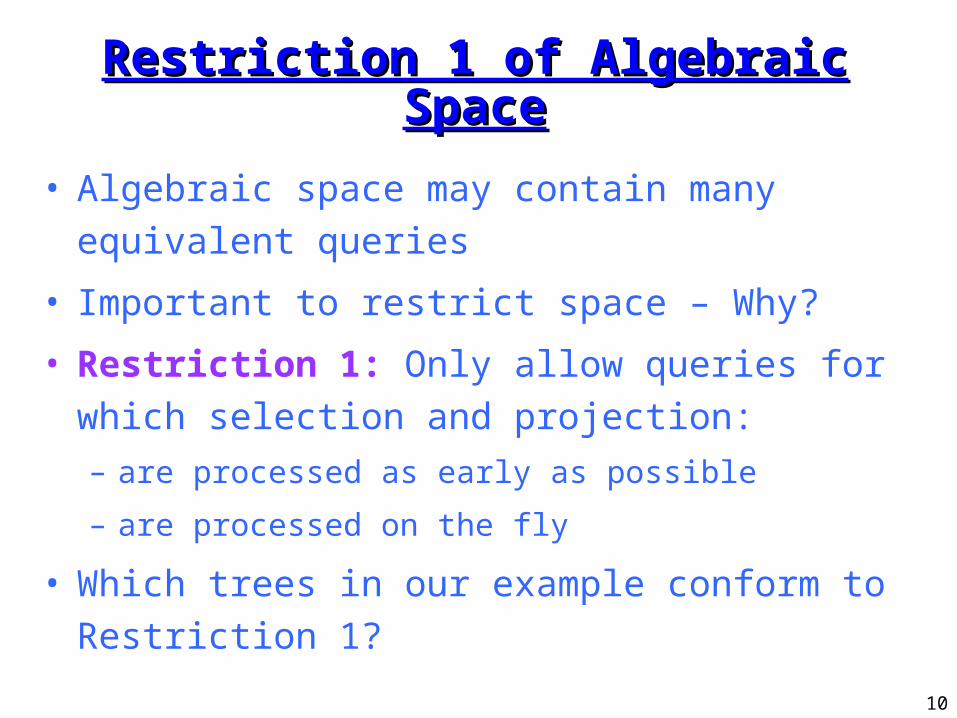
Restriction 1 of Algebraic Restriction 1 of Algebraic SpaceSpace
• Algebraic space may contain many equivalent queries
• Important to restrict space – Why?
• Restriction 1: Only allow queries for which selection and projection:– are processed as early as possible
– are processed on the fly
• Which trees in our example conform to Restriction 1?

11
Performing Selection and Performing Selection and Projection "On the Fly"Projection "On the Fly"
• Selection and projection are performed as part of other actions
• Projection and selection that appear one after another are performed one immediately after another
Projection and Selection do not require writing to the disk
• Selection is performed while reading relations for the first time
• Projection is performed while computing answers from previous action
12
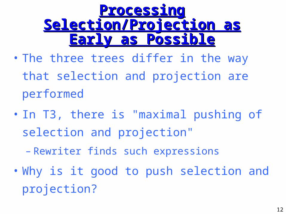
Processing Processing Selection/Projection as Selection/Projection as
Early as PossibleEarly as Possible• The three trees differ in the way that
selection and projection are performed
• In T3, there is "maximal pushing of
selection and projection"
– Rewriter finds such expressions
• Why is it good to push selection and
projection?

13
Restriction 2 of Algebraic Restriction 2 of Algebraic SpaceSpace
• Since the order of selection and projection is determined, we can write trees only with joins.
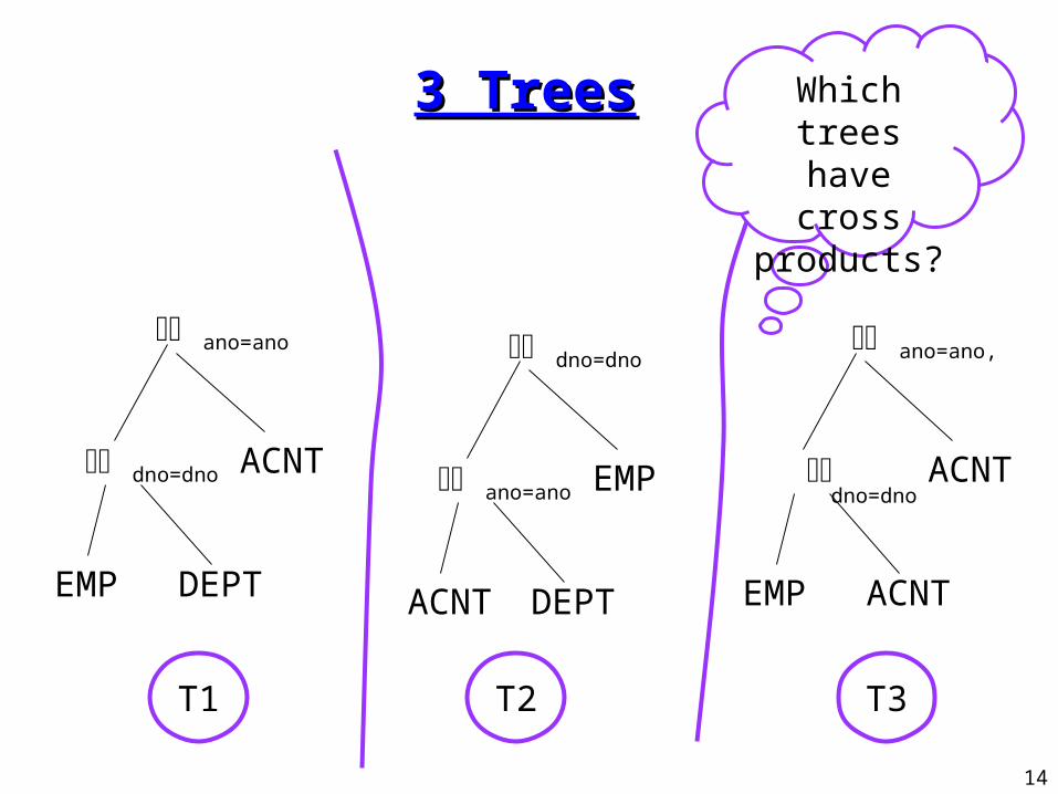
• Restriction 2: Cross products are never formed, unless the query asks for them.
• Why this restriction?
• Example:
select name, floor, balance
from emp, dept, acnt
where emp.dno=dept.dno and
dept.ano = acnt.ano
14
3 Trees3 Trees
ano=ano
EMP DEPT
T1 T2 T3
dno=dno ACNT
ano=ano,
dno=dno
EMP ACNT
ACNT
dno=dno
ACNT DEPT
ano=ano EMP
Which trees have cross products?

15
Restriction 3 of Algebraic Restriction 3 of Algebraic SpaceSpace
• The left relation is called the outer relation in a join and the right relation is the inner relation. (as in terminology of nested loops algorithms)
• Restriction 3: The inner operand of each join is a database relation, not an intermediate result.
• Example: select name, floor, balance
from emp, dept, acnt, bank
where emp.dno=dept.dno and dept.ano=acnt.ano
and acnt.bno = bank.bno

16
3 Trees3 Trees
ano=ano
EMP DEPT
T1 T2 T3
dno=dno ACNT
ano=ano
EMP DEPT
dno=dno
ACNT
Which trees follow
restriction 3?
bno=bno
BANK
BANK
bno=bno
ano=ano
EMPDEPT
dno=dno
ACNT
bno=bno
BANK

17
Algebraic Space - Algebraic Space - SummarySummary
• We allow plans that
1. Perform selection and projection early
and on the fly
2. Do not create cross products
3. Use database relations as inner relations
(also called left –deep trees)

18
PlannerPlanner
• Dynamic programming algorithm to find best plan for performing join of N relations.
• Intuition:– Find all ways to access a single relation. Estimate costs and
choose best access plan(s)
– For each pair of relations, consider all ways to compute joins using all access plans from previous step. Choose best plan(s)...
– For each i-1 relations joined, find best option to extend to i relations being joined...
– Given all plans to compute join of n relations, output the best.

19
Pipelining JoinsPipelining Joins
• Consider computing: (Emp Dept) Acnt.
In principle, we should
– compute Emp Dept, write the result to the disk
– then read it from the disk to join it with Acnt
• When using block and index nested loops
join, we can avoid the step of writing to the
disk.
• Do you understand now restriction 3?

20
Pipelining Joins - Example Pipelining Joins - Example
Read block from Emp
Find matching Dept tuples using index
Find matching Acnt tuples using index
Write final output
1
2 3
4
Emp blocks
Dept blocks
Acnt blocks
Output blocks Buffer

21
Reminder: Dynamic Reminder: Dynamic ProgrammingProgramming
• To find an optimal plan for joining R1, R2, R3, R4,
choose the best among:
– Optimal plan for joining R2, R3, R4 + for reading R1 +
optimal join of R1 with result of previous joins
– Optimal plan for joining R1, R3, R4 + for reading R2 +
optimal join of R2 with result of previous joins
– Optimal plan for joining R1, R2, R4 + for reading R3 +
optimal join of R3 with result of previous joins
– Optimal plan for joining R1, R2, R3 + for reading R4 +
optimal join of R4 with result of previous joins

22
Not Good EnoughNot Good Enough
• Example, suppose we are computing (R(A,B)
S(B,C)) T(B,D)
• Maybe merge-sort join of R and S is not the
most efficient, but the result is sorted on B
• If T is sorted on B, the performing a sort-
merge join of R and S, and then of the result
with T, maybe the cheapest total plan

23
Interesting OrdersInteresting Orders
• For some joins, such as sort-merge join, the
cost is cheaper if relations are ordered
• Therefore, it is of interest to create plans
where attributes that participate in a join are
ordered on attributes in joins later on
• For each interesting order, save the best plan.
• We save plans for non order if it better than all
interesting order costs

24
ExampleExample
• We want to compute the query:
select name, mgr
from emp, dept
where emp.dno=dept.dno and sal>30K and floor = 2
• Available Indexes: B+tree index on emp.sal, B+tree index on emp.dno, hashing index on dept.floor
• Join Methods: Block nested loops, index nested loops and sort-merge
• In the example, all cost estimations are fictional.

25
Step 1 – Accessing Single Step 1 – Accessing Single RelationsRelations
Relation Interesting
Order
Plan Cost
emp emp.dno Access through B+tree on emp.dno 700
Access through B+tree on emp.sal
Sequential scan
200
600
dept Access through hashing on dept.floor
Sequential scan
50
200
Which do we save for the next step?

26
Step 2 – Joining 2 RelationsStep 2 – Joining 2 Relations
Join
Method
Outer/Inner Plan Cost
nested
loops
empt/dno •For each emp tuple obtained through
B+Tree on emp.sal, scan dept
through hashing index on dept.floor to
find tuples matching on dno
1800
•For each emp tuple obtained through
B+Tree on emp.dno and satisfying
selection, scan dept through hashing
index on dept.floor to find tuples
matching on dno
3000

27
Step 2 – Joining 2 RelationsStep 2 – Joining 2 Relations
Join
Method
Outer/Inner Plan Cost
nested
loops
dept/emp •For each dept tuple obtained through
hashing index on dept.floor, scan emp
through B+Tree on emp.sal to find
tuples matching on dno
2500
•For each dept tuple obtained through
hashing index on dept.floor, scan emp
through B+Tree on emp.dno to find
tuples satisfying the selection on
emp.sal
1500

28
Step 2 – Joining 2 RelationsStep 2 – Joining 2 RelationsJoin
Method
Outer/
Inner
Plan Cost
sort
merge
•Sort the emp tuples resulting from
accessing the B+Tree on emp.sal into L1
•Sort the dept tuples resulting from
accessing the hashing index on dept.floor
into L2
•Merge L1 and L2
2300
•Sort the dept tuples resulting from
accessing the hashing index on dept.floor
into L2
•Merge L2 and the emp tuples resulting
from accessing the B+Tree on emp.dno
and satisfying the selection on emp.sal
2000

29
The PlanThe Plan
• Which plan will be chosen?

30
Cost ModelCost Model
• Taught In class: estimate time of
computing joins
• Now: Estimating result size

31
Estimating Result SizesEstimating Result Sizes

32
Picking a Query PlanPicking a Query Plan
• Suppose we want to find the natural join of: Reserves, Sailors, Boats.
• The 2 options that appear the best are (ignoring the order within a single join):
(Sailors Reserves) Boats
Sailors (Reserves Boats)
• We would like intermediate results to be as small as possible. Which is better?

33
Analyzing Result SizesAnalyzing Result Sizes
• In order to answer the question in the
previous slide, we must be able to estimate
the size of (Sailors Reserves) and
(Reserves Boats).
• The DBMS stores statistics about the
relations and indexes.
• They are updated periodically (not every
time the underlying relations are modified).

34
Statistics Maintained by Statistics Maintained by DBMSDBMS
• Cardinality: Number of tuples NTuples(R) in each relation R
• Size: Number of pages NPages(R) in each relation R
• Index Cardinality: Number of distinct key values NKeys(I) for each index I
• Index Size: Number of pages INPages(I) in each index I
• Index Height: Number of non-leaf levels IHeight(I) in each B+ Tree index I
• Index Range: The minimum ILow(I) and maximum value IHigh(I) for each index I

35
Estimating Result SizesEstimating Result Sizes
• Consider
• The maximum number of tuples is the product of the cardinalities of the relations in the FROM clause
• The WHERE clause is associating a reduction factor with each term
• Estimated result size is: maximum size times product of reduction factors
SELECT attribute-list
FROM relation-list
WHERE term1 and ... and termn

36
Estimating Reduction Estimating Reduction FactorsFactors
• column = value: 1/NKeys(I) if there is an index I on column. This assumes a uniform distribution. Otherwise, System R assumes 1/10.
• column1 = column2: 1/Max(NKeys(I1),NKeys(I2)) if there is an index I1 on column1 and I2 on column2. If only one column has an index, we use it to estimate the value. Otherwise, use 1/10.
• column > value: (High(I)-value)/(High(I)-Low(I)) if there is an index I on column.

37
ExampleExample
• Cardinality(R) = 1,000 * 100 = 100,000
• Cardinality(S) = 500 * 80 = 40,000
• NKeys(Index on R.agent) = 100
• High(Index on Rating) = 10, Low = 0
SELECT *
FROM Reserves R, Sailors S
WHERE R.sid = S.sid and S.rating > 3 and
R.agent = ‘Joe’

38
Example (cont.)Example (cont.)
• Maximum cardinality: 100,000 * 40,000
• Reduction factor of R.sid = S.sid: 1/40,000
• Reduction factor of S.rating > 3: (10–3)/(10-
0) = 7/10
• Reduction factor of R.agent = ‘Joe’: 1/100
• Total Estimated size: 700