Quenching of Reaction by Cellular Flows

Albert Fannjiang∗ Alexander Kiselev† Lenya Ryzhik ‡

September 27, 2004

Abstract

We consider a reaction-diffusion equation in a cellular flow. We prove that in the strongflow regime there are two possible scenario for the initial data that is compactly supportedand the size of the support is large enough. If the flow cells are large compared to thereaction length scale, propagating fronts will always form. For the small cell size, any finitelysupported initial data will be quenched by a sufficiently strong flow. We estimate that theflow amplitude required to quench the initial data of support L0 is A > CL4

0 ln(L0). Theessence of the problem is the question about the decay of the L∞ norm of a solution to theadvection-diffusion equation, and the relation between this rate of decay and the propertiesof the Hamiltonian system generated by the two-dimensional incompressible fluid flow.

1 Introduction

It has been well understood since the classical work of G.I. Taylor that the presence of a fluid flowmay greatly increase the mixing properties of diffusion. This phenomenon is known as “eddydiffusivity” or “enhanced diffusion”. The mathematical approach to the problem is usually viathe homogenization techniques that concentrate on the long time-large scale behavior: see [25]for a recent extensive review. This approach is appropriate when there are no other time scales inthe problem so that one may wait as long as needed for the mixing effects to become prominent.

Recently there has been a lot of interest in the effect of flows on the qualitative and quantita-tive behavior of solutions of reaction-diffusion equations. Intuitively, there may be two oppositeeffects of the additional mixing by the flow: on one hand, it may increase the spreading rate ofthe chemical reaction (the “wind spreading the fire” effect), or it may extinguish the reaction(the “try to light the campfire in a wind” effect). The first effect is related to the behavior offront-like solutions, and has been extensively studied recently: traveling fronts have been shownto exist in various flows [5, 6, 7, 33, 34, 35, 36], and flows have been shown to speed-up the frontpropagation due to the improved mixing [3, 4, 9, 20, 37], see [4, 36] for recent reviews of themathematical results in the area. This problem has also attracted a significant attention in the

∗Department of Mathematics, University of California, Davis, CA 95616, USA; e-mail: cafan-njiang@ucdavis.edu

†Institute for Advanced Study, Princeton, NJ 08540 and Department of Mathematics, University of Wisconsin,Madison, WI 53706, USA; e-mail: kiselev@math.wisc.edu

‡Department of Mathematics, University of Chicago, Chicago, IL 60637; e-mail: ryzhik@math.uchicago.edu

1

physical literature, we mention [1, 2, 3, 17, 18, 19, 22, 23] among the recent papers and referto [30] as a general reference. The present paper addresses the second phenomenon mentionedabove: the possibility of flame extinction by a flow. The basic idea is that if the reaction processmay occur only at the temperatures T above a critical threshold θ0, then mixing by a strongflow coupled to diffusion may drop the temperature everywhere below θ0 and hence extinguishthe flame. However, unlike the usual linear advection-diffusion homogenization problems, onemay not wait for this to happen beyond the time tc it takes for the chemical reaction to occur –the mixing has to happen before this time. The question we address is: ”Given a threshold θ0,a time tc, and the support L0 of the initial data, can we find a flow amplitude A0(L0) so that ifthe flow amplitude A > A0(L0) is sufficiently large then supx T (t = tc,x) ≤ θ0?” This problemhas been first considered in [10] for unidirectional, or shear, flows that have open streamlines.Even in this simple situation the answer is non-trivial: in order for quenching to be possible,the profile u(y) should not be constant on intervals larger than a prescribed size. The answerhas been shown to be sharp in [21].

In this paper, we study quenching by a different class of flows with a more complex structure:incompressible cellular flows. These are flows such that the whole plane R2 is separated intoinvariant regions bounded by the separatrices of the flow that connect the flow saddle points.Many types of instabilities in fluids lead to cellular flows, making them ubiquitous in nature.We only mention Rayleigh-Benard instability in heat convection, Taylor vortices in Couette flowbetween rotating cylinders or heat expansion driven Landau-Darrieus instability. The fact thatthe cellular flows have closed streamlines make the effect of advection more subtle. An importantrole in the possibility of quenching is played by a thin boundary layer which forms along theseparatrices of the flow. Our main results show that the cellular flow is quenching if and only ifthe size of the minimal invariant regions (the flow cells) is smaller than a certain critical size ofthe order of laminar flame length scale.

The simplest mathematical model that describes a chemical reaction in a fluid is a singleequation for temperature T of the form

Tt + Au(x) · ∇T = ∆T + Mf(T ) (1)T (0,x) = T0(x)

where the flow u(x) is prescribed. We are interested in the effect of a strong advection, andaccordingly have written the velocity as a product of an amplitude A and a fixed flow u(x). Inthis paper we consider nonlinearity of the ignition type, that is, we assume that

(i) f(T ) is Lipschitz continuous on 0 ≤ T ≤ 1,

(ii) f(1) = 0, ∃θ0 such that f(T ) = 0 for T ∈ [0, θ0], f(T ) > 0 for T ∈ (θ0, 1) (2)(iii) f(T ) ≤ T.

The threshold θ0 is called the ignition temperature. The last condition in (2) is just a nor-malization. We consider the reaction-diffusion equation (1) in a two-dimensional strip D =x ∈ R, y ∈ [0, 2πl] with the periodic boundary conditions at the vertical boundaries:

T (x, y + 2πl) = T (x, y).

2

The initial data T0(x) = T (0,x) is assumed to satisfy 0 ≤ T0(x) ≤ 1. The maximum principleimplies that then 0 ≤ T (t,x) ≤ 1 for all t ≥ 0. We will say that regions with temperature closeto one are ”hot”, and those with temperature close to zero are ”cold”.

The problem of extinction and flame propagation in (1) with the ignition type nonlinearity(2) was first studied by Kanel [16] in one dimension and with no advection. Assume for simplicitythat the initial data are given by a characteristic function: T0(x) = χ[0,L](x). Kanel showed that,in the absence of fluid motion, there exist two length scales L0 < L1 such that the flame becomesextinct for L < L0, and propagates for L > L1. More precisely, he has shown that there existL0 and L1 such that

T (t,x) → 0 as t →∞ uniformly in D if L < L0 (3)T (t,x) → 1 as t →∞ for all (x, y) ∈ D if L > L1.

In the absence of advection, the flame extinction is achieved by diffusion alone, given that thesupport of initial data is small compared to the scale of the laminar front width lc = M−1/2.However, in many applications quenching is a result of strong wind, intense fluid motion andoperates on larger scales. Kanel’s result was extended to non-zero advection by shear flows byRoquejoffre [31] who has shown that (3) holds also for u 6= 0 with L0 and L1 depending, inparticular, on A and u(y) in an uncontrolled way.

As we have mentioned, the question of the dependence of the strength of advection A whichis necessary for quenching the initial data of a given size L0 has been recently studied in [10] and[21] in the case of a unidirectional (shear) flow (Au(y), 0). Following [10], we call the flow u(x, y)quenching if for every L0 there exists A0(L0) such that the solution of (1) with the initial dataof size L0 and advection strength A > A0(L0) quenches. It turns out [10, 21] that the shear flowu(y) is quenching if and only if u(y) does not have a plateau of size larger than a certain criticalthreshold (comparable with the length scale M−1/2 which characterizes the width of a laminarflame). The intuition behind this result is that shear flows are very effective in stretching thefront and exposing the hot initial data to cool-off effects of diffusion unless there is a long, flatpart in their profile, where this phenomenon is obviously not present.

Here we consider (1) for the domain D = R × [−πl, πl] with the 2πl-periodic boundaryconditions in y and decay conditions in x:

T (t, x, y) = T (t, x, y + 2πl), T (t, x, y) → 0 as x → ±∞. (4)

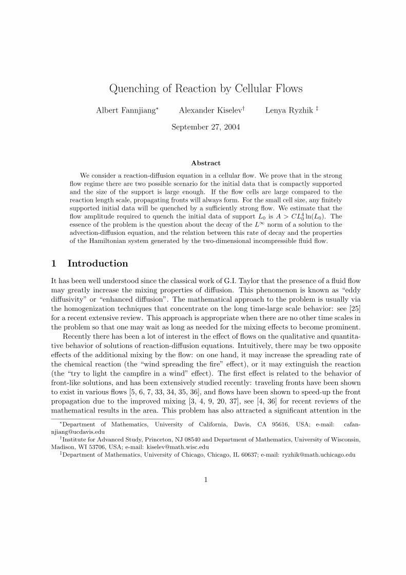
We restrict ourselves to a particular example of a cellular flow u(x, y) that has the form ul(x, y) =∇⊥hl(x, y), where ∇⊥h = (hy,−hx). Here l defines the size of a flow cell, and we take the streamfunction hl to be

hl(x, y) = l sinx

lsin

y

l(5)

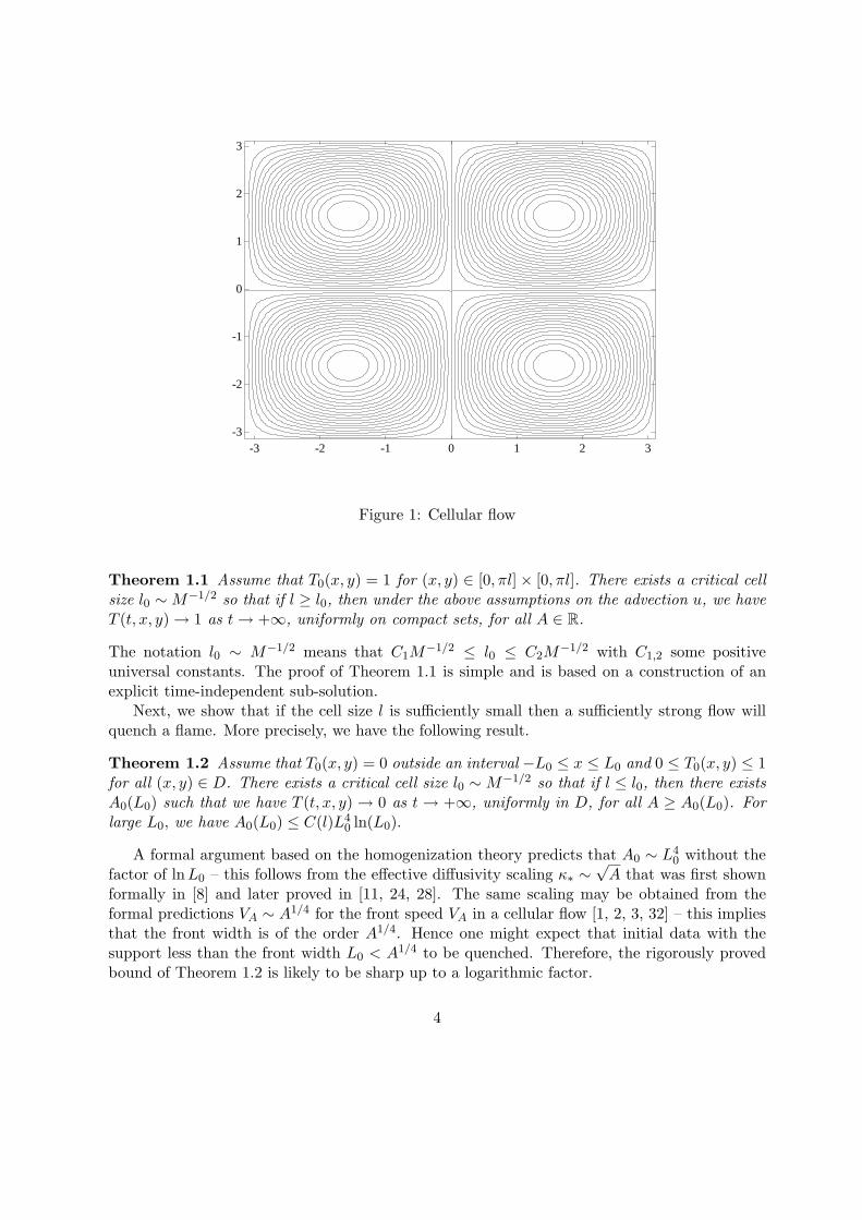
whose streamline structure are shown in Fig. 1.We will usually omit the index l in notation for ul, hl for the fluid flow; it will be clear from

the context what the scaling is. The initial data T0(x, y) is non-negative, and bounded aboveby one: 0 ≤ T0(x, y) ≤ 1.

The first theorem shows that cellular flows with large cells do not have the quenching prop-erty.

3

-3

-2

-1

0

1

2

3

-3 -2 -1 0 1 2 3

Figure 1: Cellular flow

Theorem 1.1 Assume that T0(x, y) = 1 for (x, y) ∈ [0, πl]× [0, πl]. There exists a critical cellsize l0 ∼ M−1/2 so that if l ≥ l0, then under the above assumptions on the advection u, we haveT (t, x, y) → 1 as t → +∞, uniformly on compact sets, for all A ∈ R.

The notation l0 ∼ M−1/2 means that C1M−1/2 ≤ l0 ≤ C2M

−1/2 with C1,2 some positiveuniversal constants. The proof of Theorem 1.1 is simple and is based on a construction of anexplicit time-independent sub-solution.

Next, we show that if the cell size l is sufficiently small then a sufficiently strong flow willquench a flame. More precisely, we have the following result.

Theorem 1.2 Assume that T0(x, y) = 0 outside an interval −L0 ≤ x ≤ L0 and 0 ≤ T0(x, y) ≤ 1for all (x, y) ∈ D. There exists a critical cell size l0 ∼ M−1/2 so that if l ≤ l0, then there existsA0(L0) such that we have T (t, x, y) → 0 as t → +∞, uniformly in D, for all A ≥ A0(L0). Forlarge L0, we have A0(L0) ≤ C(l)L4

0 ln(L0).

A formal argument based on the homogenization theory predicts that A0 ∼ L40 without the

factor of lnL0 – this follows from the effective diffusivity scaling κ∗ ∼√

A that was first shownformally in [8] and later proved in [11, 24, 28]. The same scaling may be obtained from theformal predictions VA ∼ A1/4 for the front speed VA in a cellular flow [1, 2, 3, 32] – this impliesthat the front width is of the order A1/4. Hence one might expect that initial data with thesupport less than the front width L0 < A1/4 to be quenched. Therefore, the rigorously provedbound of Theorem 1.2 is likely to be sharp up to a logarithmic factor.

4

The particular choice of the stream function (5) is not important for the proof but it doessimplify some of the estimates – it is straightforward to generalize our result to other cellularflows. However, the proof of Theorem 1.2 does use the periodicity of the flow in an essential way.We believe that the quenching property should hold for sufficiently regular non-periodic flowswith small cells as well. We have preliminary results in this direction using different techniques;however, these results give much weaker upper bound for A0(L0), and will appear elsewhere.

At the heart of the proof of Theorem 1.2 is the question about the rate of decay of L∞ norm(and its dependence on A) of the solution to a passive advection-diffusion equation. Thus, ourmain object of study is a natural question about the effects of a combination of two fundamentaland separately well-understood processes: advection by a fixed incompressible flow and diffusion.Yet their interaction is well known to produce subtle phenomena. The issues we study are directlyrelated to the work of Freidlin and Wentzell [13, 14, 15] on the random perturbations of theHamiltonian systems. They show that in the limit of large A the process converges to a diffusionon the Reeb graph of the background Hamiltonian. The relation to that work is very natural asany incompressible flow in two dimensions is a Hamiltonian system (the stream function is theHamiltonian). However, the cellular flow that we consider does not satisfy the assumptions ofthe Freidlin-Wentzell theory, which requires growth of the Hamiltonian at infinity and does notallow existence of hetero-clinic orbits. Nevertheless, one may restate the small cell assumptionin Theorem 1.2 as a requirement that the Reeb graph of the Hamiltonian has a sufficientlysmall diameter in its natural metric. The proof of Theorem 1.2 is based on two observations:first, temperature becomes approximately constant on the whole skeleton of separatrices, as theskeleton is just one point on the Reeb graph. Because of that, solution inside each cell maybe split into two parts. One solves the initial value problem with zero data on the boundary.Another solves a nearly identical boundary value problem in each cell. The first part decaysbecause the cell is small – this is where we use the size restriction. The second one is nearlyidentical on all cells, hence it has to be small in order not to violate the preservation of theL1-norm. The technical part of the proof is in making this informal scenario rigorous.

The paper is organized as follows: in Section 2 we prove Theorem 1.1 by constructing anappropriate sub-solution and using certain PDE estimates to prove convergence of solution tounity. In Section 3 we give the proof of Theorem 1.2, which is more involved. It uses uniform inA estimates on the evolution of advection-diffusion equation, a boundary layer argument, andprobabilistic estimates for an auxiliary cell heating problem.Acknowledgment. The research of AF is supported in part by The Centennial Fellowshipfrom American Mathematical Society and U.S. National Science Foundation (NSF) grant DMS-0306659. AK has been supported in part by NSF grants DMS-0321952 and DMS-0314129. LRhas been supported in part by NSF grant DMS-0203537 and ONR grant N00014-02-1-0089.Both AK and LR acknowledge support by Alfred P. Sloan fellowships.

2 Absence of quenching by large cells

We prove in this section Theorem 1.1, that is, we show that cellular flows with sufficiently largecells do not have the quenching property. The proof consists of two steps. First, we construct a

5

time-independent sub-solution Φ(x) to (1) in a cell C1 = [0, πl]× [0, πl]: the function Φ satisfies

Aul (x) · ∇Φ ≤ ∆Φ + Mf(Φ) (6)

and is 2πl-periodic in y. It is also positive on an open set inside C1 and negative on ∂C1. Wenormalize Φ so that Φ ≤ 1. As T0 = 1 on C1 by assumption, we have T0(x) ≥ Φ(x). Then themaximum principle implies that T (t,x) ≥ Φ(x) for all t ≥ 0 and x ∈ C1. It follows that T (t,x)does not vanish as t → +∞. In the second step we show that actually T (t,x) → 1. We beginwith the construction of the sub-solution Φ(x). First, we rescale equation (1) by x → lx so thata sub-solution in the rescaled coordinates should satisfy

A

lu(x) · ∇Φ ≤ 1

l2∆Φ + Mf(Φ). (7)

Lemma 2.1 If l is sufficiently large then there exists a C1 function Φ(x) that is constant onthe streamlines of the flow u(x) and satisfies (7) for x ∈ C1 = [−π, π]2. Moreover, Φ(x) ≤ 1 forall x ∈ C1, and Φ(x) < 0 for x ∈ ∂C1.

Proof of Lemma 2.1. We may choose two numbers θ1 and θ2 so that θ0 < θ1 < θ2 < 1 andsuch that the straight line that connects the point (θ1, 0) to the point (θ2, f(θ2)) lies below thegraph of f(T ). More precisely, that means that the function

g(T ) =

0, T ≤ θ1

α(T − θ1), θ1 ≤ T ≤ θ2

f(T ), T ≥ θ2

(8)

with α = f(θ2)/(θ2 − θ1), satisfies g(T ) ≤ f(T ). Such modification of f(T ) for the constructionof sub-solutions was first used in [16], and then in [10]. A function Φ(h(x)) satisfies (7) if

1l2

(|∇h|2 d2Φ

dh2+ ∆h

dΦdh

)+ Mg(Φ) ≥ 0,

where h(x, y) = sinx sin y is the stream function. Note that the advection term vanishes identi-cally for such functions. We use the fact that ∆h = −2h to obtain

|∇h|2 d2Φdh2

− 2hdΦdh

+(

l

lc

)2

g(Φ) ≥ 0. (9)

Here lc = M−1/2 is the laminar front width, the length scale associated to the chemical reactionstrength. Relation (9) indicates that the ratio l/lc has to be sufficiently large for a sub-solutionto exist. Note that

2h(1− h) ≤ |∇h|2 ≤ 2(1− h2).

Indeed, we have

|∇h(x, y)|2 = sin2 x cos2 y + cos2 x sin2 y = sin2 x + sin2 y − 2 sin2 x sin2 y

≥ 2 sinx sin y(1− sinx sin y) = 2h(x, y)(1− h(x, y))

6

and

|∇h(x, y)|2 ≤ 2− 2 sin2 x sin2 y = 2(1− h2(x, y)).

Therefore it suffices to construct an increasing function Φ(h) satisfying

d2Φdh2

− 2h

2h(1− h)dΦdh

+1

2(1− h2)

(l

lc

)2

g(Φ) ≥ 0,

which would in turn follow from

d2Φdh2

− 11− h

dΦdh

+12

(l

lc

)2

g(Φ) = 0.

Make a change of variables R =l

lc√

2(1− h) so that the above becomes

d2ΦdR2

+1R

dΦdR

+ g(Φ) = 0. (10)

The center of the cell corresponds now to R = 0, while the boundary h = 0 becomes R =l

lc√

2.

We impose the following “initial data” for (10):

Φ(0) = θ2,dΦ(0)dR

= 0.

The explicit form (8) of the function g(Φ) implies that the solution Φ(R) is given explicitly by

Φ(R) = θ1 + (θ2 − θ1)J0

(R√

α), for R ≤ R1 =

ξ1√α

(11)

with α as in (8). Here J0(ξ) is the Bessel function of order zero, and ξ1 is its first zero.Furthermore, we have

Φ(R) = B lnR2

R, for R1 ≤ R. (12)

The constants B and R2 are determined by matching the functions (11) and (12), and theirderivatives at R = R1. Then we get

B = (θ2 − θ1)ξ1|J ′0(ξ1)|, R2 = ξ1

√θ2 − θ1

f(θ2)exp

[θ1

(θ2 − θ1)ξ1|J ′0(ξ1)|]

.

Observe that the function Φ(R) constructed above is negative on the boundary of the cell only

provided that R2 <l

lc√

2, which means that the cell size

l ≥ lc√

2ξ1

√θ2 − θ1

f(θ2)exp

[θ1

(θ2 − θ1)ξ1|J ′0(ξ1)|]

7

has to be sufficiently large for this construction to be applicable. This proves Lemma 2.1. ¤In order to finish the proof of Theorem 1.1 we have to show that T (t,x) → 1 as t → +∞

provided that T0(x) = 1 on a cell. For such initial data we have

T0(x) ≥ Φ0(x) = max Φ(h(x)), 0 ,

where the function Φ(x) is the sub-solution constructed in Lemma 2.1. It follows from theparabolic maximum principle that then T (t,x) ≥ Φ0(x) for all t ≥ 0. Furthermore, we haveT (t,x) ≥ Ψ(t,x), where the function Ψ(t,x) satisfies (1) with the initial data Φ0(x). Notethat Ψ(t,x) ≥ Φ0(x) for all t ≥ 0. The maximum principle applied to the finite differencesΨh(t, x) = Ψ(t + h,x) − Ψ(t,x) implies that Ψ(t,x) is a point-wise increasing function of timethat is bounded above by one. Therefore the point-wise limit Ψ(x) = limt→+∞Ψ(t,x) exists,moreover, Ψ(x) ≥ Φ0(x), and Ψ(x) satisfies the stationary problem

Au(x) · ∇Ψ = ∆Ψ + Mf(Ψ). (13)

with the 2πl-periodic boundary conditions in y

Ψ(t, x, 0) = Ψ(t, x, 2πl)

(here 2N is the number of cells in y direction). We have the following lemma.

Lemma 2.2 The function Ψ(x, y) satisfies the following bound:∫

D|∇Ψ(x)|2 dx +

∫

Df(Ψ(x)) dx < +∞, (14)

where D = Rx × [−πl, πl]y.

Proof. The function Ψ(t,x) satisfies an a priori bound

1τ

∫ τ

0

(∫

Df(Ψ(t,x)) dx

)dt ≤ C0, τ ≥ CM−1,

that may be easily proved as in [9]. Here the constant C0 may depend on the flow amplitude A.Therefore, there exists a sequence of times tn → +∞ so that

∫

Df(Ψ(tn,x)) dx ≤ C0.

This implies that ∫

Df(Ψ(x)) dx ≤ C0,

and it remains to obtain the bound on ‖∇Ψ‖L2 in (14). We multiply (13) by Ψ and integratein x between −X + ζ and X + ζ with X large and ζ ∈ [0, lc], and in y ∈ R. We get

A

2

∫ πl

−πl

[u1(X + ζ, y)|Ψ(X + ζ, y)|2 − u1(−X + ζ, y)|Ψ(−X + ζ, y)|2] dy

=∫ πl

−πl

[Ψ(X + ζ, y)Ψx(X + ζ, y)−Ψ(−X + ζ, y)Ψx(−X + ζ, y)

]dy

+M

∫ πl

−πldy

∫ X+ζ

−X+ζΨ(x, y)f(Ψ(x, y))dx−

∫ πl

−πldy

∫ X+ζ

−X+ζ|∇Ψ(x, y)|2dx

8

and average this equation in ζ ∈ [0, lc]. This provides the bound

1lc

∫ lc

0dζ

∫ πl

−πldy

∫ X+ζ

−X+ζ|∇Ψ(x, y)|2dx ≤ πAl‖u‖∞ +

2πl

lc+ M

∫

Df(Ψ(x, y))dxdy

Taking X to infinity, we obtain∫

D|∇Ψ(x, y)|2dx ≤ πAl‖u‖∞ +

2πl

lc+ M

∫

Df(Ψ(x, y))dxdy

and the bound on ∇Ψ in (14) follows. ¤Now we are ready to complete the proof of Theorem 1.1.

Proof. Lemma 2.2 implies that there exist two sequences of points xn → −∞ and zn → +∞so that ∫ πl

−πl

(|∇Ψ(xn, y)|2 + |∇Ψ(zn, y)|2) dy → 0 as n → +∞. (15)

We integrate (13) in y and in x between xn and zn to obtain

A

∫ πl

−πl

[u1(zn, y)Ψ(zn, y)− u1(xn, y)Ψ(xn, y)

]dy (16)

=∫ πl

−πl

[Ψx(zn, y)−Ψx(xn, y)

]dy + M

∫ πl

−πldy

∫ zn

xn

f(Ψ(x, y))dx.

We pass to the limit n →∞ in (16). Observe that∣∣∣∣∫ πl

−πlΨx(zn, y)dy

∣∣∣∣ ≤√

πl

(∫ πl

−πl|Ψx(zn, y)|2dy

)1/2

→ 0 as n → +∞

as follows from (15), and similarly∣∣∣∣∫ πl

−πlΨx(xn, y)dy

∣∣∣∣ → 0 as n → +∞.

Furthermore, since ∫ πl

−πlu1(x, y)dy = 0

for all x ∈ R, (15) and the Cauchy-Schwartz inequality imply that∫ πl

−πlu1(zn, y)Ψ(zn, y)dy =

∫ πl

−πlu1(zn, y)

(∫ y

0Ψξ(zn, ξ)dξ

)dy → 0, as n → +∞.

Therefore in the limit n → +∞ equation (16) becomes∫

Df(Ψ(x, y))dxdy = 0

and hence f(Ψ(x, y)) = 0 for all (x, y) ∈ D. However, since Ψ(x, y) ≥ Φ0(x, y), while, on theother hand, max Φ0(x, y) = θ2 > θ0, and the function Ψ(x, y) is continuous, we conclude thatΨ(x, y) ≡ 1. This finishes the proof of Theorem 1.1. ¤

9

3 Quenching by small cells

In this section we show that the cellular flow with small cells is quenching. The proof proceedsin several steps. First, we reduce the problem to a linear advection-diffusion equation. Indeed,as f(T ) ≤ T we have the following upper bound for T :

T (t,x) ≤ eMtφ(t,x). (17)

The function φ(t,x) satisfies the advection-diffusion equation

∂φ

∂t+ Au · ∇φ = ∆φ (18)

with the same initial data φ(0,x) = T0(x) and the 2πl-periodic boundary conditions in y:φ(t, x, y) = φ(t, x, y + 2πl). Note that if at some time t0 > 0 we have φ(t0,x) ≤ θ0 everywhere,then the maximum principle implies that φ(t,x) ≤ θ0 and T satisfies the linear equation (18)for all t ≥ t0. Then the conclusion of Theorem 1.2 follows. Hence, the upper bound (17) impliesthat it suffices to show φ(t = M−1, x, y) ≤ θ′0 = θ0e

−1 and this is what we will do.Heuristically, the proof relies on the observation that solution of (18) should generally become

constant along the streamlines of the flow if its amplitude is large. Moreover, the value of thesolution on the streamlines h = h0 very near the boundary in two neighboring cells have tobe close (as follows from a simple L2-bound on ∇φ appearing in Lemma 3.3 below). However,that means that solution should have, roughly speaking, the same profile in each cell. This isincompatible with the preservation of the L1-norm of φ unless this function is very small in eachof the cells which means that solution has to be less than θ0 everywhere. The proof follows thisheuristic outline – the technical difficulty is that we are able to control the uniformity of thesolution along the streamlines only in a space-time averaged sense. Additional ingredients arerequired to obtain the point-wise control.

3.1 The Nash inequality lemma

We will need throughout the proof an L1−L∞ decay estimate for solutions of the linear diffusion-advection

∂T

∂t+ v · ∇T = ∆T (19)

that is independent of the advection strength. Equation (19) is considered in the infinite stripD = R× [−πl, πl] with the 2πl-periodic boundary conditions in y direction.

Lemma 3.1 There exists a constant C > 0 so that the solution of

∂ψ

∂t+ v · ∇ψ = ∆ψ (20)

ψ(0,x) = ψ0(x) ≥ 0, x ∈ R2

with the 2πl-periodic boundary condition in y and a flow v that is 2πl-periodic, sufficiently regularand divergence-free: ∇ · v = 0, satisfies

‖ψ(t)‖L∞(D) ≤ Cn2(t)‖ψ0‖L1(D), (21)

10

where D = Rx × [−πl, πl]y. Here n(t) is the unique solution of

4n4(t)1 + 4n3(t)l3

=C1

l2t,(22)

and the constants C, C1 do not depend on v.

Remark. Note that (22) implies that for t ≥ l2, we have n(t)2 ∼ Cl√

t. Hence, solution decays

as the solution of the one-dimensional problem after the time it takes the diffusion to feel theboundary.

Proof. We multiply (20) by ψ and integrate over the domain D to obtain

12

d

dt‖ψ‖2

2 = −‖∇ψ‖22. (23)

Here and below in the proof of this Lemma, ‖ · ‖p denotes the norm in Lp(D).We now prove the following version of the Nash inequality [27] for a strip of width l:

‖∇ψ‖22 ≥ C

l2‖ψ‖62

‖ψ‖41 + l3‖ψ‖1‖ψ‖3

2

(24)

The proof of (24) is similar to that of the usual Nash inequality. We represent ψ in terms of itsFourier series-integral:

ψ(x, y) =∑

n∈Z

∫

Reiny/l+ikxψn(k)

dk

(2π)2,

whereψn(k) =

1l

∫

De−ikx−iny/lψ(x, y)dxdy.

Therefore we have |ψn(k)| ≤ 1l‖ψ‖L1 . The Plancherel formula becomes

∫

D|ψ(x, y)|2dxdy =

∑

n,m∈Z

∫

R2

einy/l−imy/l+ikx−ipxψn(k)ψm(p)dkdpdxdy

(2π)4

= l∑

n∈Z

∫|ψn(k)|2 dk

(2π)2

and similarly∫

D|∇ψ(x, y)|2dxdy = l

∑

n∈Z

∫

R

(k2 +

n2

l2

)|ψn(k)|2 dk

(2π)2.

Let ρ > 0 be a positive number to be chosen later. Then using the Plancherel formula we maywrite

‖ψ‖22 = I + II,

whereI = l

∑

|n|≤ρl

∫

|k|≤ρ|ψn(k)|2 dk

2π≤ Clρ([lρ] + 1)

l2‖ψ‖2

1 ≤Cρ(lρ + 1)

l‖ψ‖2

1.

11

The rest may be bounded by

II ≤ l

ρ2

∑

n∈Z

∫

k∈R

(k2 +

n2

l2

)|ψn(k)|2 dk

(2π)2≤ C

ρ2‖∇ψ‖2

2.

Therefore we have for all ρ > 0:

‖ψ‖22 ≤

Cρ(lρ + 1)l

‖ψ‖21 +

C

ρ2‖∇ψ‖2

2.

We choose ρ so that

ρ3 =l‖∇ψ‖2

2

‖ψ‖21

and obtain

‖ψ‖22 ≤

C‖∇ψ‖2/32

l2/3‖ψ‖2/31

(l4/3‖∇ψ‖2/3

2

‖ψ‖2/31

+ 1

)‖ψ‖2

1 +C‖∇ψ‖2

2‖ψ‖4/31

l2/3‖∇ψ‖4/32

=2C

l2/3‖ψ‖4/3

1 ‖∇ψ‖2/32 + Cl2/3‖∇ψ‖4/3

2 ‖ψ‖2/31 .

This is a quadratic inequality ax2+bx−c ≥ 0 with x = ‖∇ψ‖2/32 , a = l2/3‖ψ‖2/3

1 , b =2

l2/3‖ψ‖4/3

1 ,

and c = ‖ψ‖22/C and hence

x ≥ −b +√

b2 + 4ac

2a=

2c

b +√

b2 + 4ac≥ c√

b2 + 4ac.

This implies that

‖∇ψ‖2/32 ≥ C‖ψ‖2

2

(4‖ψ‖8/3

1

l4/3+ 4l2/3‖ψ‖2/3

1 ‖ψ‖22

)−1/2

and therefore

‖∇ψ‖22 ≥ C‖ψ‖6

2

(4‖ψ‖8/3

1

l4/3+ 4l2/3‖ψ‖2/3

1 ‖ψ‖22

)−3/2

≥ C‖ψ‖62

(‖ψ‖41

l2+ l‖ψ‖1‖ψ‖3

2

)−1

≥ Cl2‖ψ‖62

‖ψ‖41 + l3‖ψ‖1‖ψ‖3

2

.

Hence (24) indeed holds.We insert (24) into the inequality (23) and using the conservation of the L1-norm of ψ (recall

that the initial data is non-negative) obtain

d‖ψ‖2

dt≤ − Cl2‖ψ‖5

2

‖ψ0‖41 + l3‖ψ0‖1‖ψ‖3

2

. (25)

12

Integrating (25) in time we have

Cl2t ≤ ‖ψ0‖41

4‖ψ‖42

+l3‖ψ0‖1

‖ψ‖2≤ 1

z(t)

[l3 +

14z3(t)

],

where z(t) = ‖ψ(t)‖2/‖ψ0‖1, and thus

4z4(t)1 + 4l3z3(t)

≤ 1Cl2t

. (26)

The function on the left side of (26) is monotonically increasing and hence we have

‖ψ(t)‖2 ≤ n(t)‖ψ0‖1, (27)

where n(t) is the solution of (22).Let us denote by Pt the solution operator for (20): ψ(t) = Ptψ0. Then (27) implies that

‖Pt‖L1→L2 ≤ n(t). The adjoint operator P∗t is the solution operator for

∂ψ

∂t− v · ∇ψ = ∆ψ (28)

ψ(0, x) = ψ0(x), x ∈ Rd

Note that the preceding estimates rely only on the skew adjointness of the convection operatorv · ∇. Therefore we have the bound ‖P∗t ‖L1→L2 ≤ n(t) and hence ‖Pt‖L2→L∞ ≤ n(t) so that

‖ψ(t)‖L∞ ≤ n(t/2)‖ψ(t/2)‖L2 ≤ n2(t/2)‖ψ0‖L1 (29)

and the proof of Lemma 3.1 is complete. ¤A very similar argument leads to an estimate for the solution of (19) with the 2πl-periodic

or zero Dirichlet boundary conditions in both x and y. We state this variant which we will need.

Lemma 3.2 Consider equation (20) with the 2πl-periodic boundary conditions in x and y. As-sume that the initial data ψ0(x) is mean zero:

∫ψ0(x) dx = 0. Then there exists a constant

C > 0 such that‖ψ(t)‖L∞(D) ≤ Cn2(t)‖ψ0‖L1(D),

where D = [0, 2πl]x × [0, 2πl]y. Here n(t) is the unique solution of

4n4(t)1 + 4n3(t)l3

=C1

l2t,

and the constants C, C1 do not depend on v. The same result holds for the zero Dirichlet boundaryconditions, without the assumption that the initial data is mean zero.

13

3.2 Variation of temperature on streamlines and gradient bounds

The next step of the proof is to estimate the time-space averages of the oscillations of the solutionalong the streamlines of u and show that they are small if the advection amplitude is sufficientlystrong. This does not have to be true in general, but a bound of this type holds if the initialdata is uniform on the streamlines – then one has only to show that no large oscillations appearat later times. First, we reduce the problem to such initial data with the help of the Nashinequality in Lemma 3.1. The maximum principle implies that it suffices to prove Theorem 1.2for the initial data of the form T0 = 1 for |x| ≤ L0 and T0 = 0 elsewhere. We split the initialdata as

T0(x) = T0(x)η(h(x)/δ0) + T0(x)(1− η(h(x)/δ0)) = φ01 + φ02. (30)

The small parameter δ0 will be specified later. The cutoff function η(h) satisfies

0 ≤ η(h) ≤ 1 for all h ∈ R, η(h) = 0 for |h| ≤ 1, η(h) = 1 for |h| ≥ 2.

We split the solution φ(t,x) of (18) as a sum φ = φ1 + φ2. The functions φ1,2 satisfy (18) withthe initial data φ01 and φ02, respectively. The function φ01 is smooth and is constant (1 or 0)on the streamlines of the flow. In particular it is equal to zero in the whole “water-pipe” systemof boundary layers around the separatrices. The function φ02 satisfies a bound

‖φ02‖L1(D) ≤ |x ∈ D = R× [−πl, πl] : |x| ≤ L0, |h(x)| ≤ 2δ0| ≤ Cδ0L0 ln(l/δ0). (31)

Therefore, Lemma 3.1 implies that if L0 is sufficiently large and we require that

δ0 ≤ Cθ0l2

L0(ln(L0/l))2, (32)

with an appropriate constant C, then the function φ2 satisfies a uniform upper bound

‖φ2(t = l2)‖L∞(D) ≤θ′010

. (33)

Hence we choose δ0 as in (32) and concentrate on the function φ1 that is initially uniform alongthe streamlines of u. We drop the subscript one to simplify the notation wherever this causesno confusion.

Next, we obtain some uniform estimates for solutions of (18) that are initially constant onthe streamlines.

Lemma 3.3 For any time t > 0 we have∫ t

0

∫

D|∇φ|2dxds ≤

∫

D|φ0(x)|2dx. (34)

Assume in addition that the initial data φ0(x) for the equation (18) are constant on streamlines.Then ∫ t

0

∫

D|u · ∇φ|2dxds ≤ CA−2t

∫

D|∆φ0|2dx + CA−1

∫

D|φ0|2dx. (35)

14

Proof. Multiplying (18) by φ(t,x) and integrating we trivially obtain∫

D|φ(t,x)|2dx +

∫ t

0

∫

D|∇φ(s,x)|2dxds =

∫

D|φ0(x)|2dx,

which implies (34). Next, we multiply (18) by u · ∇φ and integrate over D to get∫

D|u · ∇φ|2dx = A−1

∫

Du · ∇φ(∆φ− φt)dx

≤ 12A2

∫

Dφ2

t dx +12

∫

D|u · ∇φ|2dx−A−1

∫

D∇φT∇u∇φdx.

Thus we get ∫

D|u · ∇φ|2 dx ≤ CA−2

∫

Dφ2

t dx + CA−1

∫

D|∇φ|2dx. (36)

From (36) and (34) we obtain that∫ t

0

∫

D|u · ∇φ(x, s)|2 dxds ≤ CA−2

∫ t

0

∫

Dφ2

sdxds + CA−1

∫

D|φ0|2dx. (37)

Recall that initially φ0(x, y) is constant on streamlines of u, so that u · ∇φ0 = 0. Since thefunction φt satisfies the same equation (18) as φ, this implies that

∫

D|φt(t,x)|2dx +

∫ t

0

∫

D|∇φt(s,x)|2dxds =

∫

D|φt(0,x)|2dx =

∫

D|∆φ0|2dx.

Therefore, bounding from above the time derivative term in (37), we arrive at (35). ¤Note that the initial data for the function φ1 in (30) obeys an upper bound

∫

D|∆φ01|2dx =

∫ L0

−L0

∫ 2πl

0

∣∣∣∣∆[η

(h(x)δ0

)]∣∣∣∣2

dydx

=∫ L0

−L0

∫ 2πl

0

∣∣∣∣∆h(x)

δ0η′

(h(x)δ0

)+|∇h(x)|2

δ20

η′′(

h(x)δ0

)∣∣∣∣2

dxdy ≤ CL0

δ30

ln(

l

δ0

).

Hence, according to (35), the total oscillation on streamlines is bounded by∫ t

0

∫

D|u · ∇φ(s,x)|2 dxds ≤ CA−2t

∫

D|∆φ01|2dx + CA−1

∫

D|φ01|2dx (38)

≤ CA−2τL0

δ30

ln(

l

δ0

)+ CA−1L0

for t ≤ τ .

15

3.3 Boundary layer and cell-to-cell heat conduction

Lemma 3.3 suggests that for most times, there should be very little temperature variation alongthe streamlines. Our next goal is make this statement more precise. Let us fix a time τ to bechosen later. We will denote by h and θ the coordinates inside each cell, with h being our usualstream function and θ the orthogonal coordinate normalized by the condition |∇θ| = |∇h| alongthe cell boundary and increasing in the direction of the flow. Let δ > 0 be an arbitrary, smallnumber to be chosen later.

Lemma 3.4 There exists h0 satisfying 2δ > h0 > δ such that∫ τ

0

∑

cells

supθ1,θ2|φ(h0, θ1, t)−φ(h0, θ2, t)|2 dt ≤ Cδ−1A−1L0l ln

(l

δ

)(A−1τδ−3

0 ln(

l

δ0

)+1) (39)

where δ0 satisfies (32). As a consequence, given a small number γ > 0, for all times except fora set Sγ of Lebesgue measure at most γτ we have

∑

cells

supθ1,θ2|φ(h0, θ1, t)−φ(h0, θ2, t)|2 ≤ Cδ−1A−1γ−1L0l ln

(l

δ

)(A−1δ−3

0 ln(

l

δ0

)+ τ−1). (40)

Proof. It is easy to check that

∂φ

∂θ= |∇h|−1|∇θ|−1u · ∇φ.

Let us denote by Sa the streamline h = a ∈ [δ, 2δ] in a given cell. Then we have

supθ1,θ2|φ(h, θ1)− φ(h, θ2)|2 ≤

(∫

Sh

|u · ∇φ| dθ

|∇θ||∇h|)2

≤ C

∫

Sh

|u · ∇φ|2 dθ

|∇θ||∇h|∫

Sh

dθ

|∇θ||∇h| ≤ Cl lnl

δ

∫

Sh

|u · ∇φ|2 dθ

|∇θ||∇h| .

The last step follows from the estimate∫

Sh

dθ

|∇θ||∇h| ≤ Cl ln(

l

δ

)

in the tube δ < h < 2δ. Integrating in h and in time and summing over all cells, we obtain∫ τ

0

∫ 2δ

δ

∑

cells

supθ1,θ2|φ(h, θ1, t)− φ(h, θ2, t)|2 dhdt ≤ Cl ln

(l

δ

)∫ τ

0

∫

D|u · ∇φ|2 dxdt. (41)

Now (39) and (40) follow from (38) by an application of the mean value theorem. ¤We see that for all times but a small set of ”exceptional” times, the value of the temperature

on the h = h0 streamline is close to some constant in any cell. Our next goal is to establisha control on how different these constants can be for two neighboring cells. Consider two suchcells, C− and C+, and let B be their common boundary. Let us choose the coordinates on these

16

two cells so that h = 0 on B, h > 0 on the right cell C+, h < 0 on the left cell C−, and theangular coordinates θ− and θ+ are equal to zero in the mid-point of B. Denote by D± the regionbounded by curves θ−,+ = ±y and streamlines h = ±h0, where y ∼ l is chosen so that D± issufficiently far away from the corners of the cells (so that |∇h|, |∇θ±| ≥ C on D±). Also denoteby S−,+ the pieces of streamlines bounding D±. Let us define the temperature drop between C−and C+ as follows:

|φ+ − φ−| = max0, minS+φ−maxS−φ, minS−φ−maxS+φ

.

Note that if the time is not exceptional, Lemma 3.4 implies that maximum and minimum of φalong h = h0 streamline in any cell differ by at most Cδ−1A−1l ln(l/δ)γ−1L0(A−1δ−3

0 ln(l/δ0) +τ−1). Now we are ready to state

Lemma 3.5 For any τ > 0, we have for D = R× [−πl, πl]∫ τ

0

∑

cells

|φ+ − φ−|2 dt ≤ Cδl−1

∫ τ

0

∫

D|∇φ|2 dxdt ≤ CL0δ. (42)

Therefore, given γ > 0, for all times with an exception of a set of Lebesgue measure at most γτ,we have ∑

cells

|φ+ − φ−|2 ≤ CδL0γ−1τ−1. (43)

Proof. The proof is straightforward and has already appeared in [20]. We sketch it here for thesake of completeness. Clearly,

∣∣∣∣∫ h0

−h0

∂φ

∂h(h, θ) dh

∣∣∣∣ ≥ |φ+ − φ−|,

for any θ± = θ. Since in the region D± we have |∇h|, |∇θ±| ∼ 1, integrating in the curvilinearcoordinates we obtain

∫

D|∇φ|2dx ≥

∫ y

−y

∫ h0

−h0

∣∣∣∣∂φ

∂h

∣∣∣∣2

dθdh ≥ Cδ−1l|φ+ − φ−|2,

finishing the proof. ¤Lemmas 3.4 and 3.5 allow to control how much the temperature changes from cell to cell.

Our next lemma summarizes this in a way that will prove useful.

Lemma 3.6 Assume that at a certain time t, the estimates (40) and (43) hold. Suppose thatthere exists a cell C such that φ(h0, θ) ≥ β > 0 at some point (h0, θ) ∈ C. Then for at least Ncells, we have φ(h0, θ) ≥ β/2 for any θ inside these cells, where the number N can be estimatedfrom below as follows:

N ≥ Cβ2γτ(δL0 + δ−1A−2L0δ

−30 l ln(l/δ)τ ln(l/δ0) + δ−1A−1L0l ln(l/δ)

)−1. (44)

17

Proof Consider a cell C1 which is the closest to C and such that there exists a point (h0, θ) ∈ C1

with φ(h0, θ) < β/2. Then we must have∑

cells

|φ+ − φ−|+∑

cells

supθ1,θ2|φ(h0, θ1)− φ(h0, θ2)| > β/2, (45)

where the sum is over all cells between C and C1. On the other hand, Lemmas 3.4 and 3.5 implythat

∑

cells

|φ+ − φ−|2 +∑

cells

supθ1,θ2|φ(h0, θ1)− φ(h0, θ2)|2 (46)

≤ Cγ−1τ−1(δL0 + δ−1A−1L0l ln(l/δ)(A−1δ−30 τ ln(l/δ0) + 1)).

Since N∑N

m=1 a2n ≥

(∑Mm=1 an

)2, a combination of (45) and (46) yields (44). ¤

Now we can explain the strategy of the proof of Theorem 1.2 in more detail. Assume that ata certain ”good” (not exceptional in the sense of Lemmas 3.4, 3.5) time we have a sufficientlyhigh temperature φ = β in some cell on a streamline h = h0. Then an appropriate choice of δ(hence h0) and an application of Lemma 3.6 ensure that φ ≥ β/2 in many cells. Assume thatfor a sufficiently large portion of times ≤ τ , the temperature at h = h0 streamlines is high inmany cells. Clearly, the interiors of the cells will heat up too, giving (for a suitable choice of δensuring N is large enough) a contradiction with the preservation of the L1 norm of φ. On theother hand, if the temperature on the streamline h = h0 is low most of the time, we expect thesolution inside the cells to be small and quenching to happen if the cells are sufficiently small –the last condition ensures that the interaction between the boundary and the interior of the cellhappens on a short time scale. To make the above plan work, we need a good understanding ofan auxiliary ”cell heating” problem. The next section is devoted to this goal.

3.4 An auxiliary cell heating problem

Consider a domain Ω which is a sub-domain of a cell, defined by the condition |h| ≥ |h0|, that is,Ω is the interior of the closed streamline h = h0. We consider the following initial-boundaryvalue problem on Ω :

wt + Au · ∇w −∆w = 0 (47)w(t,x) = σ(t), x ∈ ∂Ω

w(x, 0) = g(x).

Here σ(t) is some (smooth) function of time, independent of x. Let us derive a compact formulafor the solution of (47). Set v = w−σ(t). Then v satisfies the zero Dirichlet boundary conditions,and we have

vt + Au · ∇v −∆v = −σ′(t), v(x, 0) = g(x)− σ(0).

Let us denote by H the differential operator −∆ + Au · ∇ with the zero Dirichlet boundaryconditions on ∂Ω and by e−tH the positive semigroup generated by H. Using the Duhamelformula, we get

v(t,x) = e−tH(g − σ(0)1)−∫ t

0e−(t−s)H1σ′(s) ds. (48)

18

Here the semigroup is applied to a function equal identically to one in all of Ω, denoted by 1.Integrating by parts in (48), and recalling that w = v + σ(t), we obtain

w(t,x) = e−tHg(x) +∫ t

0σ(s)He−(t−s)H1 ds. (49)

It will be convenient to use probabilistic interpretation of (49). Recall that we can representthe semigroup action in the following way (see, e.g. [12]):

e−tHf(x) = Ex [f(Xxt (ω))] ,

where Xxt is the diffusion process corresponding to H starting at x, and the expectation Ex

is taken over all paths that start at x and never leave Ω up to time t. The latter restrictioncorresponds to the zero Dirichlet boundary condition on ∂Ω. Note that in the case f ≡ 1, thefunction Q(t,x) = e−tH1 coincides with probability that the stochastic process Xx

t (ω) neverleaves Ω before time t :

e−tH1 = Ex [1(Xxt (ω))] = P(Xx

s (ω) ∈ Ω, ∀ s ≤ t).

In terms of the function Q(t,x) expression (49) becomes

w(t,x) = e−tHg(x)−∫ t

0σ(s)∂tQ(t− s,x) ds (50)

In order to control the solution of an auxiliary cell problem, we need to control the propertiesof Q(t,x), uniformly in the flow amplitude A – this is akin to Lemma 3.1. The first result weneed in this direction is the following lemma, showing that the exit probability is bounded fromabove by a constant independent of A.

Lemma 3.7 For any t satisfying 0 ≤ t ≤ C1l2 we have

∫

ΩQ(t,x) dx ≥ C2l

2 > 0, (51)

where C2 is a universal constant depending only on C1 but not on A or l.

Proof. Let us rewrite the generator H in the natural coordinates h, θ :

H = |∇θ|2 ∂2

∂θ2+ |∇h|2 ∂2

∂h2+ ∆h

∂

∂h+ (∆θ −A|∇θ||∇h|) ∂

∂θ.

Note that ∆h = −2l−2h – this property is by no means crucial for our analysis but it doessimplify some computations. The diffusion process Xx

t corresponding to H, written in the(h, θ)-coordinates, is given by

dXht =

√2|∇h|dB

(1)t − 2l−2Xh

t dt (52)

dXθt =

√2|∇θ|dB

(2)t + (∆θ −A|∇h||∇θ|)dt,

19

where the values of all functions are taken at a point (Xht , Xθ

t ), while B(1) and B(2)t are inde-

pendent one-dimensional Brownian motions. Clearly, Q(t,x) ≥ P (Xh(x)s ∈ [0, l], ∀ s ≤ t). It is

not difficult to see that the exit probabilities of Xht are majorized by the exit probabilities of the

Ornstein-Uhlenbeck process where the factor |∇h| in (52) is dropped. Indeed, let us introduce

α(t, ω) =√

2|∇h(Xht (ω), Xθ

t (ω))|.

Multiplying (52) with e2l−2t and integrating leads to

e2l−2tXh(x)t = h(x) +

∫ t

0e2l−2sα(s, ω)dB(1)

s .

Making a random time change (see, e.g., [29]), we find that the integral above has the samedistribution as the Brownian motion B0

ρ(t,ω), where

ρ(t, ω) =∫ t

0e4l−2s|α(s, ω)|2 ds.

Since |α(s, ω)|2 ≤ 2, we have

ρ(t, ω) ≤ ρ(t) ≡ 12l2(e4l−2t − 1),

and thereforeQ(t,x) ≥ P (Bh(x)

ρ(s) e−2l−2s ∈ [0, l], ∀ s ≤ t). (53)

Let us remark that the expression on the right hand side is exactly the exit probability forthe Ornstein-Uhlenbeck process mentioned above. The claim of the lemma now follows from asimple rescaling τ = t/l2, Yτ = l−1Xl2τ . ¤

Next, we need some information on the behavior of ∂tQ(t,x).

Lemma 3.8 For any t satisfying C1l2 ≥ t ≥ 0, we have

∫

Ω∂tQ(t,x)dx ≤ −C3,

with a constant C3 > 0 that depends on C1 but is independent of A or l. Moreover,∫Ω ∂tQ(t,x)dx

is monotonically increasing in time.

Proof. According to the previous lemma,∫

ΩQ(t,x) dx ≡ ‖Q(t,x)‖L1 ≥ C2l

2 > 0

for any t ≤ C1l2. The Cauchy-Schwartz inequality then implies a lower bound for the L2 norm:

‖Q(t,x)‖L2 ≥ C2l. Recall that the function Q(t,x) solves

∂Q

∂t= HQ(t,x)

20

with the zero Dirichlet boundary conditions and the initial condition Q(0,x) = 1. Then

12∂t‖Q‖2

L2 = −‖∇Q‖2L2 ≤ −l−2‖Q‖2

L2 (54)

by the Poincare inequality. Thus we have∫

QQtdx ≤ −C22 where C2 is independent of A and l.

It is clear that 0 ≤ Q(t,x) ≤ 1, and also that ∂tQ(t,x) ≤ 0 since Q(t,x) is the probability thatthe diffusion process starting at x does not exit Ω before time t. This implies the first statementof the lemma.

To prove the second statement, we use again the monotonic decay of Q(t,x) in time. Fixingsome time t > 0 and integrating by parts (using the fact that the flow u is tangent to ∂Ω) wefind that ∫

Ω∂tQ(t,x) dx =

∫

∂Ω

∂Q

∂nds.

Since the function Q vanishes on the boundary and decays (in time) inside, we see that∫Ω ∂tQdx

is monotonically increasing in time. ¤

Corollary 3.9 The solution w(t,x) of (47) with any nonnegative boundary and initial datasatisfies ∫

Ωw(t,x)dx ≥ C

∫ t

0σ(s) ds, (55)

where C is a positive constant depending on t but not on A. If t ≤ C1l2, the constant C can be

chosen independent of l.

Proof. The corollary follows immediately from the previous lemma and the representation (50).¤

Since we have no control over what happens at a small set of exceptional times, we need anestimate from above on how much the L1 norm of the solution can change if the boundary datais close to one for a short time. The second part of Lemma 3.8 implies that it is sufficient to lookat the situation when this hot period occurs at the end of the interval [0, t]. More precisely, ifwe replace σ(t) by its monotonically increasing rearrangement then the L1-norm of the solutionincreases. The following lemma will be useful in such scenario.

Lemma 3.10 For a time t satisfying 0 < t < l2, we have∫

Ω(1−Q(t,x)) dx ≤ Cl2(tl−2)1/2 ln

(l2

t

). (56)

Proof. Note that∫

Ω(1−Q(t,x)) dx =

∫

ΩP(∃ s < t : Xx

s (ω) /∈ Ω) dx.

It follows from the proof of Lemma 3.7 that the probability on the right hand side is majorizedby

P(∃ s < t : Bh(x)ρ(s) e−2l−2s /∈ [0, l]) ≤ P(∃ s < t : B

h(x)ρ(s) /∈ [0, l]), (57)

21

where ρ(t) = 12 l2(e4l−2t − 1). Take a constant C so that ρ(t) ≤ Ct for any t as in the statement

of the lemma. Let t = tl−2 be the rescaled time. Then the probability on the right hand side of(57) does not exceed the probability that B0

s leaves the interval C−1/2[−h/l, 1− h/l] before thetime t. Using the reflection principle, we can estimate this probability from above by one, if h/l

or 1− h/l are less than√

t, and by Cn(tl/h)n otherwise (where n > 0 is arbitrary). Integratingand taking into account the Jacobian of transformation between h, θ and x, we arrive at

∫

Ω(1−Q(t,x)) dx ≤ Cl(tl2)1/2 ln

(Cl

(tl2)1/2

)= Clt1/2 ln

(Cl2

t1/2

),

which is nothing but (56). ¤

3.5 Proof of Theorem 1.2

Now we are ready to complete the proof of Theorem 1.2. In this proof, we will work with thetime scale τ = C0l

2 for a sufficiently large universal constant C0. It means that in all estimatesof the previous sections that we are going to use, we take τ = C0l

2. This ensures, in particular,applicability of Lemma 3.8 and Corollary 3.9. If we show that φ(t,x) ≤ θ′0/2 = θ0/(2e) for somet ≤ τ, this will be sufficient for quenching since we assume that τ ≤ τc = M−1 (small cell size).

Proof. We have a set Sγ of exceptional times of size at most γτ such that on the complementSc

γ of Sγ the estimates (40), (43) are valid. The value of the constant γ will be chosen later andwill be independent of A and l. Assume first that for all t ∈ Sc

γ except for a set Sb (of “bad”times) of size at most γτ we have φ(h0, θ) ≤ γ for all cells and all θ. We are going to showthat if γ is chosen sufficiently small (with the choice being uniform in A, l), then we must havequenching. Let Ωn be the subset of a cell Cn enclosed by |h| = |h0|. Then for any x ∈ Ωn wehave φ(t,x) ≤ φ(t,x) where φ(t,x) satisfies

φt −∆φ + Au · ∇φ = 0

with the initial data φ(x, 0) = 1 in Ωn, and the boundary data given by

φ(s,x)|h=h0 =

1, s ∈ Sγ ∪ Sb;γ, otherwise

.

This bound on φ follows from the representation formula (50) and the above assumption on thebehavior of φ(h0, θ). By linearity, inside each region Ωn, we have φ(t,x) = φ1(t,x) + φ2(t,x),where φ1 satisfies the zero Dirichlet boundary conditions, while φ2 has zero initial data. Lett1 = C1l

2, where C1 is a universal constant which will be chosen below. A simple argumentusing (54) shows that

l−2‖φ1(t1, ·)‖L1(Ωn) ≤ l−1‖Φ1(t1, ·)‖L2(Ωn) → 0 (58)

uniformly in A, l as C1 →∞.The function φ2 can be estimated in the L1-norm using (cf. (50))

φ2(t,x) = −∫ t

0σ(s)∂tQ(t− s,x)ds

22

and the second statement in Lemma 3.8 as

‖φ2(t1, ·)‖L1(Ωn) ≤ −∫ t1

0σ(s)

∫

Ωn

∂t1Q(t1 − s,x)dxds

≤ −∫ t1

t1−|Sγ∪Sb|

∫

Ωn

∂t1Q(t1 − s,x)dxds− γ

∫ t1−|Sγ∪Sb|

0

∫

Ωn

∂tQ(t1 − s,x)dxds

≤∫

Ωn

[1−Q(|Sγ ∪ Sb|,x)] dx + γ

∫

Ωn

[1−Q(t1,x)] dx

≤ Cl2[(C1γ)1/2 ln

(1

C1γ

)+ C1γ

](59)

by Lemma 3.10.It follows now from the parabolic maximum principle that for all times t ≥ t1, the solution

φ(t,x) of the original linear advection-diffusion problem (18) in any cell Cn satisfies

φ(t,x) ≤ φ∗(t,x) + φ2(t,x).

The function φ2 has been estimated in (31) and (33). The function φ∗(t,x) solves (47) for t ≥ t1with the 2πl-periodic boundary conditions in x, y and at time t = t1 = C1l

2 is given by

φ∗(t1,x) =

φ(t1,x), x ∈ Ωn

1 x ∈ Cn \ Ωn.

Lemma 3.2 allows us to choose a positive number γ so that if

‖φ∗(t1,x)‖L1(Cn) ≤ γl2,

then‖φ∗(t1 + l2,x)‖L∞(Cn) ≤ Cn2(l2)‖φ∗(t1,x)‖L1(Cn) ≤ θ′0/4.

This is possible, as n2(l2) ∼ l−2 (see Remark after Lemma 3.1). Note that

‖φ∗(t1,x)‖L1(Cn) ≤ ‖φ1(t1,x)‖L1(Ωn) + ‖φ2(t1,x)‖L1(Ωn) + Cδl ln(l/δ).

Choosing C1 large enough we can use (58) to estimate the first term on the right hand sideand make sure it does not exceed γl2/3. Next we choose γ small enough so that (59) givessimilar control of the second term. Finally, choose δ small enough so that the last term is alsosufficiently small. With this choice of C1, γ and δ (uniform in A, l) we have

‖φ(t1 + l2,x)‖L∞ ≤ ‖φ∗(t1 + l2,x)‖L∞(Cn) + θ′0/10 ≤ θ′0/2

and thus quenching.It remains to consider the case when there exists a set of bad times Sb ∈ [0, t1] of size at

least γτ (with γ universal constant determined above) such that for any t ∈ Sb, there exists acell Cn such that for some point (h0, θ) ∈ Cn, we have φ(h0, θ) ≥ γ. We are going to show thatthis cannot be true if A is large enough, thus forcing the scenario which is considered above andleads to quenching. Indeed, Lemma 3.6 implies that there are at least

N = Cγ3τ(δL0 + δ−1A−2L0δ

−30 τ l ln(l/δ) ln (l/δ0) + δ−1A−1L0l ln(l/δ)

)−1 (60)

23

cells such that φ(h0, θ) > γ/2 for any θ in these cells. For each cell, let σ(t) = minθφ(h0, θ, t).On each cell, solve the initial-boundary value problem (47) with g = 0, and denote the solutionφ(t,x). By the parabolic maximum principle, we have that φ(t,x) ≥ φ(t,x) for |h| ≥ |h0|.Applying Corollary 3.9, we obtain

∫

Dφ(τ,x) dx ≥ C

∑

cells

∫ τ

0σ(s) ds = C

∫ τ

0

∑

cells

σ(s) ds ≥ Cγ2τN, (61)

where N is given by (60). We claim that if δ = δ(L0) is chosen to be sufficiently small andA = A(L0) sufficiently large then (61) leads to

∫

Dφ(τ,x) dx À lL0, (62)

obtaining a contradiction since the L1 norm of φ is preserved by evolution. Indeed, since γ andτ/l2 are fixed constants, it suffices to choose δ so that

δ ¿ τ2

L20l

, (63)

and then choose A so that

A À max

C(l)L0

δ3/20 δ1/2

(ln

l

δ0ln

l

δ

)1/2

,C(l)L2

0

δln

(l

δ

). (64)

Recalling the formula (32) for δ0, we discover that A > C(l)L40 ln L0 is sufficient to satisfy (64),

(63), completing the proof of Theorem 1.2. ¤

References

[1] M. Abel, A. Celani, D. Vergni and A. Vulpiani, Front propagation in laminar flows, PhysicalReview E, 64, 2001, 046307.

[2] M. Abel, M. Cencini, D. Vergni and A. Vulpiani, Front speed enhancement in cellular flows,Chaos, 12, 2003, 481.

[3] B. Audoly, H. Berestycki and Y. Pomeau, Reaction-diffusion en ecoulement stationnairerapide, C. R. Acad. Sci. Paris, 328 II, 2000, 255–262.

[4] H. Berestycki, The influence of advection on the propagation of fronts in reaction-diffusionequations, in Nonlinear PDEs in Condensed Matter and Reactive Flows, NATO ScienceSeries C, 569, H. Berestycki and Y. Pomeau eds, Kluwer, Doordrecht, 2003.

[5] H. Berestycki and F. Hamel, Front propagation in periodic excitable media, Comm. PureAppl. Math., 55, 2002, 949–1032.

[6] H. Berestycki, B. Larrouturou and P.-L. Lions, Multi-dimensional traveling wave solutionsof a flame propagation model, Arch. Rational Mech. Anal., 111, 1990, 33–49.

24

[7] H. Berestycki and L. Nirenberg, Traveling fronts in cylinders, Annales de l’IHP, Analysenon lineare, 9, 1992, 497–572.

[8] S. Childress, Alpha-effect in flux ropes and sheets, Phys. Earth Planet Inter., 20, 1979,172-180.

[9] P. Constantin, A. Kiselev, A. Oberman and L. Ryzhik, Bulk burning rate in passive-reactivediffusion, Arch. Rat. Mech. Anal., 154, 2000, 53–91.

[10] P. Constantin, A. Kiselev and L. Ryzhik, Quenching of flames by fluid advection, Comm.Pure Appl. Math 54, 2001, 1320–1342.

[11] A. Fannjiang and G. Papanicolau, Convection enhanced diffusion for periodic flows, SIAMJour. Appl. Math., 54, 1994, 333–408.

[12] M. Freidlin, Functional Integration and Partial Differential Equations, Princeton UniversityPress, Princeton 1985.

[13] M. Freidlin, Reaction-diffusion in incompressible fluid: asymptotic problems, J. Diff. Eq.,179 (2002), 44-96

[14] M. Freidlin and A. Wentzell, Random perturbations of Hamiltonian systems, Memoir AMS,1994.

[15] M. Freidlin and A. Wentzell, Random Perturbations of Dynamical Systems, 2nd ed.,Springer-Verlag, New York/Berlin, 1998.

[16] Ya. Kanel, Stabilization of solutions of the Cauchy problem for equations encountered incombustion theory, Mat. Sbornik, 59, 1962, 245–288.

[17] L. Kagan and G. Sivashinsky, Flame propagation and extinction in large-scale vortical flows,Combust. Flame, 120, 2000, 222–232.

[18] L. Kagan, P.D. Ronney and G. Sivashinsky, Activation energy effect on flame propagationin large-scale vortical flows, Combust. Theory Modelling 6, 2002, 479–485.

[19] B. Khoudier, A. Bourlioux and A. Majda, Parametrizing the burning rate speed enhance-ment by small scale periodic flows: I. Unsteady shears, flame residence time and bending,”Combust. Theory Model., 5, 2001, 295–318.

[20] A. Kiselev and L. Ryzhik, Enhancement of the traveling front speeds in reaction-diffusionequations with advection, Ann. de l’Inst. Henri Poincare, C. Analyse non lineaire, 18, 2001,309–358.

[21] A. Kiselev and A. Zlatos, Quenching of combustion by shear flows, Preprint, 2004.

[22] I. Kiss, J. Merkin and Z. Neufeld, Combustion initiation and extinction in a 2D chaoticflow, Phys. D., 183, 2003, 175–189.

25

[23] I. Kiss, J. Merkin, S. Scott, P. Simon, S. Kalliadasis, and Z. Neufeld, The structure of flamefilaments in chaotic flows, Phys. D., 176, 2003, 67–81.

[24] L. Koralov, Random perturbations of two-dimensional Hamiltonian flows, Prob. Theor. Rel.Fields, 129, 37–62, 2004.

[25] A. Majda and P. Kramer, Simplified models for turbulent diffusion: theory, numericalmodelling, and physical phenomena. Phys. Rep., 314, 1999, 237–574.

[26] J.-F. Mallordy and J.-M. Roquejoffre, A parabolic equation of the KPP type in higherdimensions, SIAM J. Math. Anal., 26, 1995, 1-20.

[27] J. Nash, Continuity of solutions of parabolic and elliptic equations, Amer. Jour. Math., 80,1958, 931–954.

[28] A. Novikov, G. Papanicolaou and L. Ryzhik, Boundary layers for cellular flows at highPeclet numbers, to appear in Comm. Pure Appl. Math., 2004.

[29] B. Oksendal, Stochastic Differential Equations, Springer-Verlag, Berlin, 1995.

[30] N. Peters, Turbulent combustion, Cambridge University Press, 2000.

[31] Roquejoffre, J.-M., Eventual monotonicity and convergence to traveling fronts for the so-lutions of parabolic equations in cylinders, Annal. Inst. Poincare, Analyse Nonlineare, 14,1997, 499-552.

[32] N. Vladimirova, P. Constantin, A. Kiselev, O. Ruchayskiy and L. Ryzhik, Flame Enhance-ment and Quenching in Fluid Flows, Combust. Theory Model., 7, 2003, 487–508

[33] V.A. Volpert and A.I. Volpert, Existence and stability of multidimensional travelling wavesin the monostable case, Israel Jour. Math., 110, 1999, 269–292.

[34] J. Xin, Existence of planar flame fronts in convective-diffusive periodic media, Arch. Rat.Mech. Anal., 121, 1992, 205–233.

[35] J. Xin, Existence and nonexistence of travelling waves and reaction-diffusion front propa-gation in periodic media, Jour. Stat. Phys., 73, 1993, 893–926.

[36] J. Xin, Analysis and modelling of front propagation in heterogeneous media, SIAM Rev.,42, 2000, 161–230.

[37] J. Xin, KPP front speeds in random shears and the parabolic Anderson model, Meth. Appl.Anal., 10, 2003, 191–198.

26