-1-

Oxford Physics Engineering Report 15LBNL-57580

Quench Protection and Magnet Power Supply RequirementsFor the MICE Focusing and Coupling Magnets

Michael A. GreenLawrence Berkeley National Laboratory

Berkeley CA 94720, USA

Holger WitteOxford University Physics Department

Oxford, OX1-3RH, UK

8 June 2005*

Abstract

This report discusses the quench protection and power supply requirements of theMICE superconducting magnets. A section of the report discusses the quench processand how to calculate the peak voltages and hotspot temperature that result from a magnetquench. A section of the report discusses conventional quench protection methods.Thermal quench back from the magnet mandrel is also discussed. Selected quenchprotection methods that result in safe quenching of the MICE focusing and couplingmagnets are discussed. The coupling of the MICE magnets with the other magnets in theMICE is described. The consequences of this coupling on magnet charging andquenching are discussed. Calculations of the quenching of a magnet due quench backfrom circulating currents induced in the magnet mandrel due to quenching of an adjacentmagnet are discussed. The conclusion of this report describes how the MICE magnetchannel will react when one or magnets in that channel are quenched.

TABLE OF CONTENTSPage

Abstract 1.Introduction 2.Quench Propagation Velocity and the Hot Spot Temperature 3.Active Quench Protection using a Resistor 9.Quench Propagation in the Magnet Coils 12.Coil Quench Back from the Aluminum Mandrel 14.Passive Quenches in the Focusing and Coupling Magnets 21.Magnetic Coupling between Various Magnets in MICE 28.Magnet Power Supply Design Parameters 34.Magnet Quench Back due to Inductive Coupling to the Mandrels 35.Concluding Comments 45.Acknowledgements 46.References 46.

* Last revision 8 May 2005

-2-

Introduction

The superconducting magnets in the MICE channel may be connected to other coilsof that in series [1], [2]. A quench of one magnet in the string will result in all magnets inthe string being dumped. A quench of one magnet may turn the other magnets in thestring normal through quench back. If the other magnets in the string are not quenchedthrough quench back, the stored magnetic energy in all of the magnets in the string willend up in the magnet that quenches. The report will discuss the advisability of hookingthe various types of magnet coils in series. Quench protection methods that allow the coilto be hooked up in series will be described.

There are two problems that are caused by the quenching of a superconductingmagnet or a string of magnets. The first problem is the need to keep the temperature ofthe magnet hot spot (the place where the magnet quench started) below about 400 K.Excessive hot spot temperatures will result in insulation failure and even a melting of theconductor. The second issue is the voltages developed turn to turn, layer to layer and toground during the quench process. Excessive voltages can cause a voltage breakdownand arcing. An arc will direct the stored energy of the magnet to the place where itoccurs and cause the coil to melt.

The two requirements of a magnet quench protection system (whether it be active orpassive) are that the hot spot temperature in the coil where the quench starts be no morethan 350 to 400 K and that the layer to layer voltage be less than say 500 V and that thevoltage to ground be less than 1500 V. (In a potted magnet, these voltage limits can beraised somewhat. Conventional quench protection methods such as putting a resistoracross the coil to extract the magnet energy will produce high voltages to ground whenthe hot spot temperatures are low and vice versa. The most desirable way to protect themagnet is quench the entire coil quickly, so that the magnet stored-energy is put into thecoils. This has the effect of reducing the hot spot temperature and reducing the voltageswithin the coil. The most desirable quench protection method for the MICE magnets isone that is completely passive. (A passive quench protection method does not need aquench detector, which in turn causes something to happen which caused the coil toquench safely.) Passive quench protection methods are inherently safe and are usuallyless expensive to implement, particularly in DC magnets.

The inductive coupling of one magnet to another affect the quench process and theway the magnet is regulated by its power supply. One cannot design a power supply for aMICE magnet or a string of MICE magnets without understanding the inductive couplingbetween the coil or coils being powered and all of the other coils in MICE.

The inductive coupling between a magnet and its mandrel can cause quench back inthe coil or any other coil in the string thus speeding up the quench process and reducingthe magnet voltages and the hot spot temperature of the coil that the quench starts in.

Inductive coupling between MICE coils can cause other coil or strings of coils notinvolved in the quench to go normal. Inductive coupling may cause all of the MICEmagnets to quench when one magnet quenches. Two factors come into play. First aquench in one magnet can cause the current in an adjacent magnet to rise above itscritical current. Second, a quench in one magnet can cause a circulating current to flowin the mandrel of an adjacent magnet. This current causes the coil wound on the mandrelto become normal through quench back.

-3-

Quench Propagation Velocity and the Hot Spot Temperature

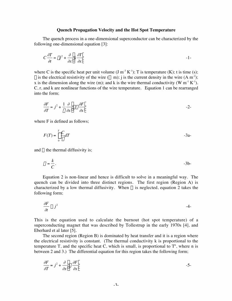
The quench process in a one-dimensional superconductor can be characterized by thefollowing one-dimensional equation [3]:

†

C ∂T∂t

= rj 2 +∂∂x

k ∂T∂x

È

Î Í ˘

˚ ˙ -1-

where C is the specific heat per unit volume (J m-3 K-1); T is temperature (K); t is time (s);r is the electrical resistivity of the wire (W m); j is the current density in the wire (A m-2);x is the dimension along the wire (m); and k is the wire thermal conductivity (W m-1 K-1).C, r, and k are nonlinear functions of the wire temperature. Equation 1 can be rearrangedinto the form;

†

∂F∂T

= j 2 +1r

∂∂x

ar∂F∂x

È

Î Í ˘

˚ ˙ -2-

where F is defined as follows;

†

F(T) =Cr0

T

Ú dT -3a-

and a the thermal diffusivity is;

†

a =kC

. -3b-

Equation 2 is non-linear and hence is difficult to solve in a meaningful way. Thequench can be divided into three distinct regions. The first region (Region A) ischaracterized by a low thermal diffusivity. When a is neglected, equation 2 takes thefollowing form;

†

∂F∂t

ª j 2 -4-

This is the equation used to calculate the burnout (hot spot temperature) of asuperconducting magnet that was described by Tollestrup in the early 1970s [4], andEberhard et al later [5].

The second region (Region B) is dominated by heat transfer and it is a region wherethe electrical resistivity is constant. (The thermal conductivity k is proportional to thetemperature T, and the specific heat C, which is small, is proportional to Tn, where n isbetween 2 and 3.) The differential equation for this region takes the following form;

†

∂F∂T

= j 2 +∂∂x

a∂F∂x

È

Î Í ˘

˚ ˙ -5-

-4-

Equation 5 takes the form that is similar to the wave equation. From this equation, acharacteristic quench velocity can be derived.

The third region (Region C) is the superconducting region characterized by zeroresisitivity. This region does not enter into the discussions of this paper. The boundarybetween regions A and B occurs at temperatures between 15 and 30 K. The boundarybetween regions B and C occurs at the transition temperature of the superconductor. Thissuperconductor transition temperature is a function of the current density in thesuperconductor j and the magnetic induction B the conductor sees.

a) The Velocity of Quench Propagation Waves along the ConductorThe velocity of normal region propagation can be found from equation 5. The

solution to this equation takes the following general form [6];

†

v < j rnanc

hnc - hno

È

Î Í

˘

˚ ˙

0.5

-6-

where rn is the resistivity of the normal metal; anc is the thermal diffusivity of the normalmetal at the superconductor critical temperature Tc; and (hnc-hno) is the change in volumeenthalpy from the superconductor operating temperature To and Tc (J m-3).

Since the specific heat per unit volume is close to that of the normal metal, thethermal diffusivity and electrical resistivity of the normal metal plus superconductor takethe following form;

†

ro = rnr +1

rand

aoc =knc

Cnc

rr +1

-7-

where r is the ratio of the normal metal to the superconductor in the overall conductor.One can modify the equation 6 to the following form;

†

v < j rokoc

Cnc (hnc - hno)È

Î Í

˘

˚ ˙

0.5

= j rnknc

Cnc (hnc - hno)È

Î Í

˘

˚ ˙

0.5

-8-

Note that equation 8 is completely independent of r. If one applies the Wiedemann Franzrelationship where r(T)k(T) = LT (L is the Lorenz number (L = 2.45 x 10-8 W W K-2)) atTc, equation 8 will take the following form;

†

v < j LTc

Cnc (hnc - hno)È

Î Í

˘

˚ ˙

0.5

. -9-

From equation 9 is clear that the normal metal thermal conductivity and electricalresistivity have almost no effect on the normal region propagation velocity.

-5-

If compares equation 9 with measurements of quench propagation velocity inmagnets, the equation changes slightly. Based on LBNL quench propagationmeasurements made in the late 1970’s on might use the following form for the equation;

†

v ª 0.6 j rnanc

hnc - hno

È

Î Í

˘

˚ ˙

0.5

ª 0.6 j LTc

Cnc (hnc - hno)È

Î Í

˘

˚ ˙

0.5

-10-

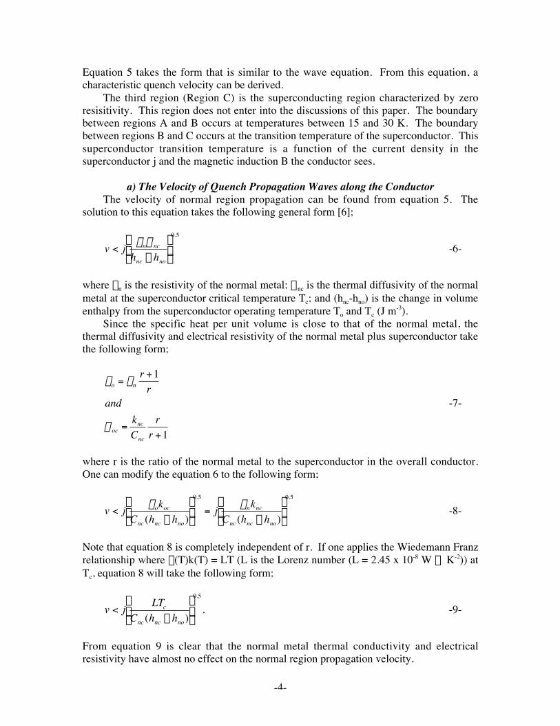
Equation 10 is dependent only on the current density in the conductor cross-section jand magnetic induction B the conductor sees. The dependence on matrix current densityis about j1.5 at low current densities. At high current densities, where heat transfer fromthe conductor plays a negligible role, the matrix current density dependence is more likej2 as observed by Scherer and Turowski [7]. (See Figure 1.) At matrix current densitiesin the range of that for the MICE magnets the dependence is more like j1.65.

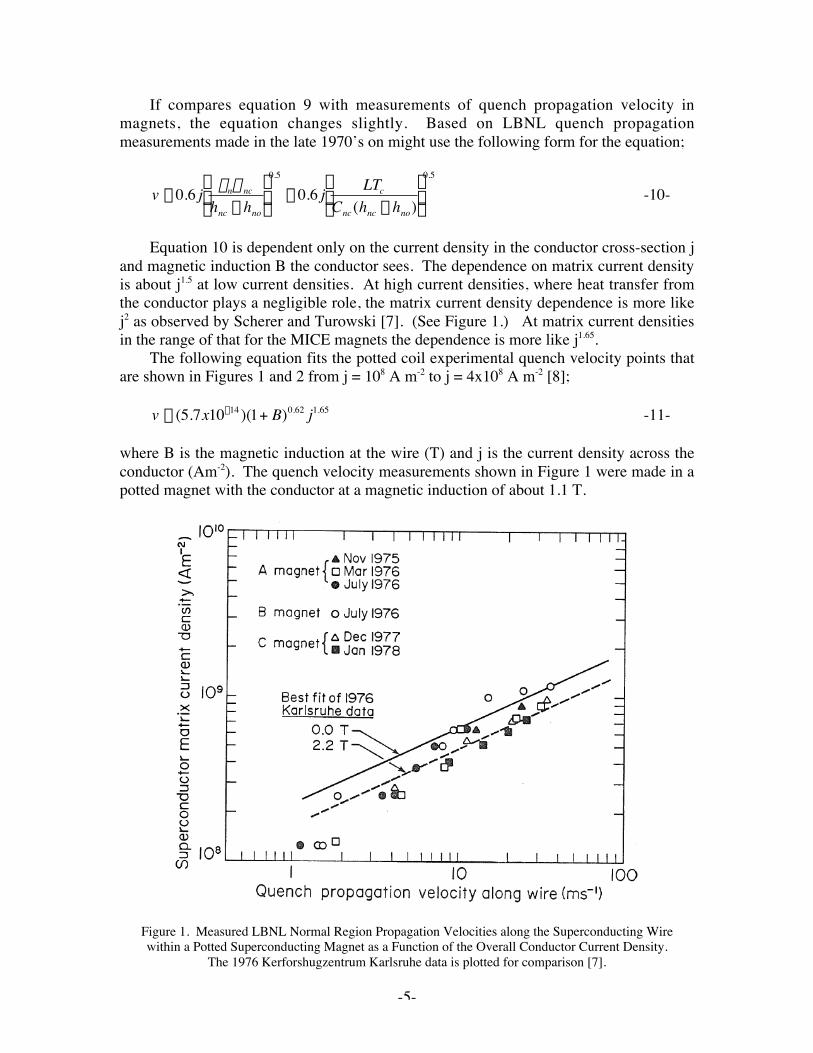
The following equation fits the potted coil experimental quench velocity points thatare shown in Figures 1 and 2 from j = 108 A m-2 to j = 4x108 A m-2 [8];

†

v ª (5.7x10-14 )(1+ B)0.62 j1.65 -11-

where B is the magnetic induction at the wire (T) and j is the current density across theconductor (Am-2). The quench velocity measurements shown in Figure 1 were made in apotted magnet with the conductor at a magnetic induction of about 1.1 T.

Figure 1. Measured LBNL Normal Region Propagation Velocities along the Superconducting Wirewithin a Potted Superconducting Magnet as a Function of the Overall Conductor Current Density.

The 1976 Kerforshugzentrum Karlsruhe data is plotted for comparison [7].

-6-

Figure 2. Predicted and Measured Quench Propagation Velocities along the Wire as aFunction of the Conductor Overall Current Density [8]

Equation 11 applies for quench propagation velocity along the superconducting wire(in the q direction in a solenoid). On can also estimate the quench propagation velocityin the other two directions using the following relationships;

†

vR = avq , -12a-

and

†

vZ = bvq . -12b-

vq is the velocity around the solenoid (in the direction of the wire); vR is the quenchvelocity in the radial direction in the solenoid; and vZ is the quench velocity along thelength of the solenoid. The dimensionless function a = vR/vq, and the dimensionlessfunction b = vZ/vq.

The values of a and b depend on the dimensions of the bare conductor and thethickness of the insulation between layers (for a) and between turns (for b). Theequations for calculating a and b for the MICE solenoid coils are as follows [9];

†

a ª 0.7 rnki

LTc

bS

r +1r

È

Î Í

˘

˚ ˙

0.5

, -13a-

and

†

b ª 0.7 rnki

LTc

aS

r +1r

È

Î Í

˘

˚ ˙

0.5

. -13b-

-7-

In equations 13a and 13b, L is the Lorentz number (L = 2.45x10-8 WWK-2.); ki is thethermal conductivity of the insulation material (For a potted magnet, ki = 0.04 Wm-1K-1.);Tc is the conductor critical temperature (use 7 K); and rn is the resistivity of the matrixmetal. (For copper, rn = 1.55x10-8/RRR in W m.) (Note: RRR is the ratio of the normalmetal resistivity at 273 K to the normal metal resistivity at 4 K.) The values of a and bare inversely proportional to the square root of RRR. S is the insulation thickness; a isthe length of the conductor (in the z direction); b is the thickness of the conductor (in ther direction); and r is the copper to superconductor ratio.

In general, a and b will have a value of 0.012 to 0.05 for a typical niobium titaniummagnet with a copper conductor with RRR from 20 to 140. From equation 9, it is clearthat RRR has almost no effect on the quench velocity along the wire. For the MICEcoupling magnet and focusing magnet, which use a bare conductor than is 0.95 mm by1.60 mm with rounded ends, the values are:

†

r direction z direction

S = 0.105 mm S = 0.08rn = 1.55x10-10 Wm rn = 1.55x10-10 Wm

a = 0.95 mm b = 1.6 mmr = 4 r = 4

a = 0.0142 b = 0.0214

The conductor proposed for the MICE magnets will have a design RRR = 100.Reducing the RRR will increase the quench propagation velocity in the r and z directions(by increasing a and b) without changing the propagation velocity in the q direction, butthere are some negative implications that make this undesirable. The reasons for wantingto keep the matrix material RRR high are as follows: 1) Having a matrix RRR that is highimprove the stability of the superconductor, particularly if the superconducting filamentsare large. 2) Having the matrix RRR high reduces the voltage buildup in the early part ofthe quench. (At the end of the quench, RRR has little effect on the voltages within thecoil.) 3) Reducing the RRR of the matrix material will reduce the integral of j2dt neededto reach the maximum allowable coil hot spot temperature. The improved quenchpropagation within the coil may end up being of little or no advantage overall.

The values of a and b given above for the MICE coils are conservative in the highfield regions of the coil because magneto resistance will increase the resistivity of thematrix material by a factor of two in the high field regions of both coils. The value of Tcwill also be reduced. Both effects will increase the values of a and b in the high fieldregions of the MICE coils by about 50 percent. Because a and b are lower in the lowfield regions of the coil the use of the values given above would be prudent.

b) The Derivation of the Conductor Burnout ConditionThe conductor burn out condition (maximum hot spot temperature) is a function of

the properties of the conductor for a given value of the integral of j2dt. When one designsthe magnet quench protection system, limiting the maximum hot spot temperature is themost important part of the quench protection system design.

The limit for the burnout condition for a superconducting magnet is derived byintegrating equation 4;

-8-

†

F = j 2

0

t

Ú dt . -14-

Redefining this equation slightly from the basic definition for F given by equation 3a, onegets the following expression;

†

F *(T) =C(T)r(T)0

T

Ú dT =r +1

rj 2dt

0

t

Ú . -15-

When a magnet quenches the start for the quench is t = 0. The end at time for themagnet quench is when the current in the coil has completely decayed away t =

†

• .Using the quench time limits, the equation for F*(T) takes the following form;

†

F * (TM ) =C (T )r(T )0

T M

Ú dT =r +1

rj 2dt

0

•

Ú =r +1

rJ0

2 X(t)2 dt0

•

Ú -16-

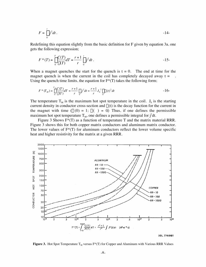
The temperature TM is the maximum hot spot temperature in the coil. J0 is the startingcurrent density in conductor cross-section and X(t) is the decay function for the current inthe magnet with time (X (0) = 1; X(•) = 0). Thus, if one defines the permissiblemaximum hot spot temperature TM, one defines a permissible integral for j2dt.

Figure 3 Shows F*(T) as a function of temperature T and the matrix material RRR.Figure 3 shows this for both copper matrix conductors and aluminum matrix conductor.The lower values of F*(T) for aluminum conductors reflect the lower volume specificheat and higher resistivity for the matrix at a given RRR.

Figure 3. Hot Spot Temperature TM versus F*(T) for Copper and Aluminum with Various RRR Values

-9-

Active Quench Protection using a Resistor

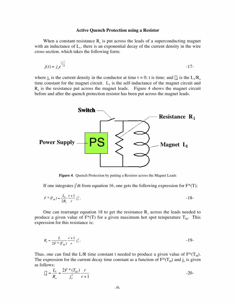
When a constant resistance Rc is put across the leads of a superconducting magnetwith an inductance of L1, there is an exponential decay of the current density in the wirecross-section, which takes the following form;

†

j(t) = joe-

tt1 -17-

where jo is the current density in the conductor at time t = 0; t is time; and t1 is the L1/Rotime constant for the magnet circuit. L1 is the self-inductance of the magnet circuit andRo is the resistance put across the magnet leads. Figure 4 shows the magnet circuitbefore and after the quench protection resistor has been put across the magnet leads.

Figure 4. Quench Protection by putting a Resistor across the Magnet Leads

If one integrates j2dt from equation 16, one gets the following expression for F*(T);

†

F * (TM ) =L1

2R1

r +1r

jo2 . -18-

One can rearrange equation 18 to get the resistance R1 across the leads needed toproduce a given value of F*(T) for a given maximum hot spot temperature TM. Thisexpression for this resistance is;

†

R1 =L

2F * (TM )r +1

rjo

2 . -19-

Thus, one can find the L/R time constant t needed to produce a given value of F*(TM).The expression for the current decay time constant as a function of F*(TM) and jo is givenas follows;

†

t1 =L1

Ro

=2F *(TM )

jo2

rr +1

-20-

-10-

The maximum voltage Vo across the leads of the magnet needed to limit the quenchmaximum hot spot temperature to TM can be calculated using the following expression;

†

Vo = ioRo =AcL

2F *(TM )r +1

rjo

3 -21-

From equations 20 and 21 one can derive the well known Ej2 limit for quenching, whichtakes the following form;

†

Eo jo2 = F *(TM )Voio

rr +1

-22-

where Eo is the fully charged stored energy of the magnet (at the start of the quench); jo isthe current density across the conductor cross-section (copper plus superconductor); andF*(TM) is the F* function for the maximum hot spot temperature TM. The quench Ej2

function is proportional to F*(TM), the maximum discharge voltage Vo and the startingcurrent Io.

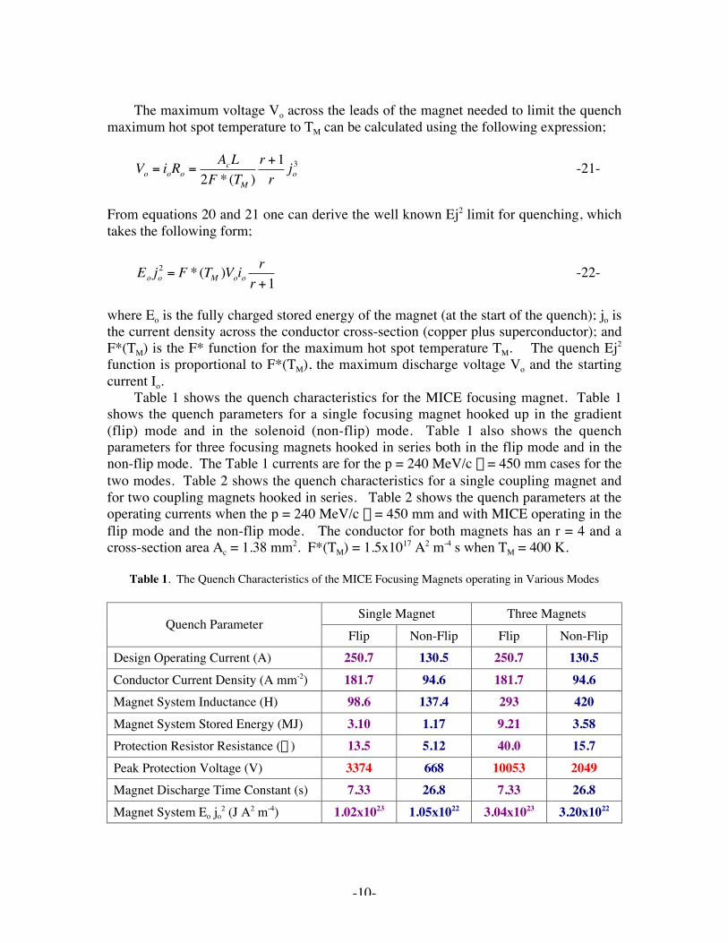
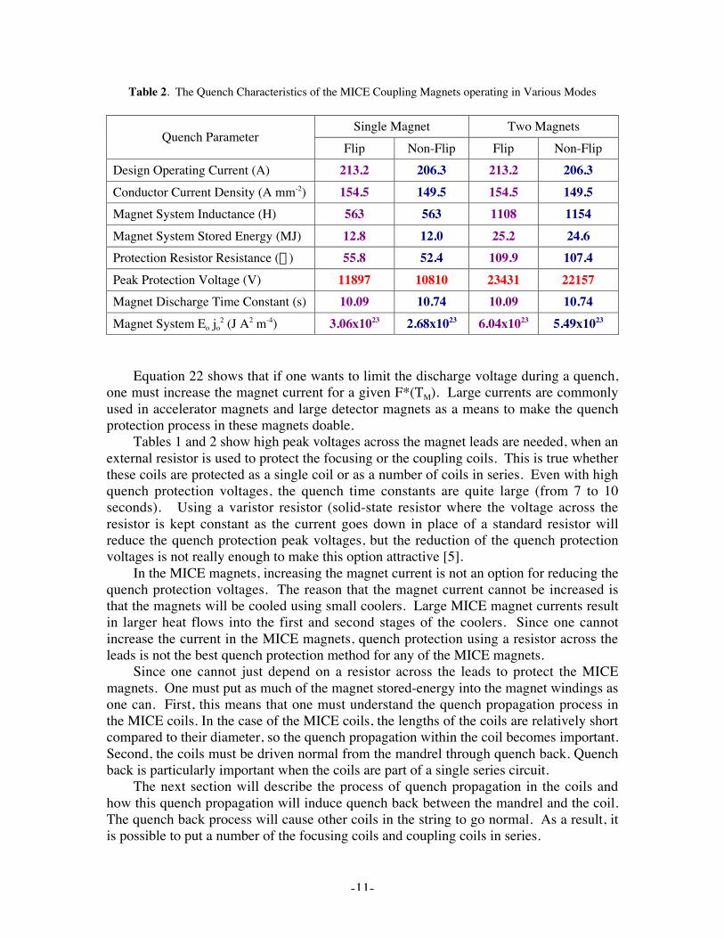
Table 1 shows the quench characteristics for the MICE focusing magnet. Table 1shows the quench parameters for a single focusing magnet hooked up in the gradient(flip) mode and in the solenoid (non-flip) mode. Table 1 also shows the quenchparameters for three focusing magnets hooked in series both in the flip mode and in thenon-flip mode. The Table 1 currents are for the p = 240 MeV/c b = 450 mm cases for thetwo modes. Table 2 shows the quench characteristics for a single coupling magnet andfor two coupling magnets hooked in series. Table 2 shows the quench parameters at theoperating currents when the p = 240 MeV/c b = 450 mm and with MICE operating in theflip mode and the non-flip mode. The conductor for both magnets has an r = 4 and across-section area Ac = 1.38 mm2. F*(TM) = 1.5x1017 A2 m-4 s when TM = 400 K.

Table 1. The Quench Characteristics of the MICE Focusing Magnets operating in Various Modes

Single Magnet Three MagnetsQuench Parameter

Flip Non-Flip Flip Non-FlipDesign Operating Current (A) 250.7 130.5 250.7 130.5Conductor Current Density (A mm-2) 181.7 94.6 181.7 94.6Magnet System Inductance (H) 98.6 137.4 293 420Magnet System Stored Energy (MJ) 3.10 1.17 9.21 3.58Protection Resistor Resistance (W) 13.5 5.12 40.0 15.7Peak Protection Voltage (V) 3374 668 10053 2049Magnet Discharge Time Constant (s) 7.33 26.8 7.33 26.8Magnet System Eo jo

2 (J A2 m-4) 1.02x1023 1.05x1022 3.04x1023 3.20x1022

-11-

Table 2. The Quench Characteristics of the MICE Coupling Magnets operating in Various Modes

Single Magnet Two MagnetsQuench Parameter

Flip Non-Flip Flip Non-FlipDesign Operating Current (A) 213.2 206.3 213.2 206.3Conductor Current Density (A mm-2) 154.5 149.5 154.5 149.5Magnet System Inductance (H) 563 563 1108 1154Magnet System Stored Energy (MJ) 12.8 12.0 25.2 24.6Protection Resistor Resistance (W) 55.8 52.4 109.9 107.4Peak Protection Voltage (V) 11897 10810 23431 22157Magnet Discharge Time Constant (s) 10.09 10.74 10.09 10.74Magnet System Eo jo

2 (J A2 m-4) 3.06x1023 2.68x1023 6.04x1023 5.49x1023

Equation 22 shows that if one wants to limit the discharge voltage during a quench,one must increase the magnet current for a given F*(TM). Large currents are commonlyused in accelerator magnets and large detector magnets as a means to make the quenchprotection process in these magnets doable.

Tables 1 and 2 show high peak voltages across the magnet leads are needed, when anexternal resistor is used to protect the focusing or the coupling coils. This is true whetherthese coils are protected as a single coil or as a number of coils in series. Even with highquench protection voltages, the quench time constants are quite large (from 7 to 10seconds). Using a varistor resistor (solid-state resistor where the voltage across theresistor is kept constant as the current goes down in place of a standard resistor willreduce the quench protection peak voltages, but the reduction of the quench protectionvoltages is not really enough to make this option attractive [5].

In the MICE magnets, increasing the magnet current is not an option for reducing thequench protection voltages. The reason that the magnet current cannot be increased isthat the magnets will be cooled using small coolers. Large MICE magnet currents resultin larger heat flows into the first and second stages of the coolers. Since one cannotincrease the current in the MICE magnets, quench protection using a resistor across theleads is not the best quench protection method for any of the MICE magnets.

Since one cannot just depend on a resistor across the leads to protect the MICEmagnets. One must put as much of the magnet stored-energy into the magnet windings asone can. First, this means that one must understand the quench propagation process inthe MICE coils. In the case of the MICE coils, the lengths of the coils are relatively shortcompared to their diameter, so the quench propagation within the coil becomes important.Second, the coils must be driven normal from the mandrel through quench back. Quenchback is particularly important when the coils are part of a single series circuit.

The next section will describe the process of quench propagation in the coils andhow this quench propagation will induce quench back between the mandrel and the coil.The quench back process will cause other coils in the string to go normal. As a result, itis possible to put a number of the focusing coils and coupling coils in series.

-12-

Quench Propagation in the Magnet Coils

Equations 11, 12a and 12b show the quench propagation velocities vq, vR, and vZwithin the magnet coils. Using these equations one can estimate the amount of timeneeded to drive the entire coil normal tMAG. The time needed to drive the entire coilnormal should be evaluated for the average magnetic induction within the coil. For boththe focusing and the coupling coil the average induction in the coil is about 2.5 T. If oneuses the average magnetic induction in the coil, the calculated time for the coil to gocompletely normal is probably conservative. The quench in most likely initiated at thehigh field point on the inner surface of the coil. At or near the high field point, thequench velocities are large. The quench will propagate around the coil and along the coil(in the z direction) rapidly. As the quench moves outward (in the r direction), it will slowdown as the field decreases; then it will speed up as the field increases.

The value of tMAG can be calculated using the following expression;

†

tMAG = tq + tR + tZ -23-

where the average value of tq and tR are;

†

tq =pRc

vq

=(1.75x1013)pRc

(1+ Bave )0.62 j1.65 , -24a-

†

tR =Tc

vR

=(1.75x1013)Tc

a(1+ Bave )0.62 j1.65 , -24b-

and the maximum value of tZ (based on the quench starting in the corner) is;

†

tZ =Lc

vZ

=(1.75x1013)Lc

b(1+ Bave )0.62 j1.65 , -24c-

where Bave is the average magnetic induction in the coil; Rc is the average radius of thecoil; Tc is the thickness of the coil; and Lc is the length of the coil. (Note: setting Lc as thelength of the coil instead of the half-length of the coil makes equation 23 even moreconservative in terms of estimating the time needed for all of the coil to go normal. Thevalues of a and b are defined by equations 13a and 13b.

For the superconductor and insulation selected for both the focusing coils and thecoupling coils, a = 0.0142, b = 0.0214, and Bave = 2.5 T. For the focusing magnet, thevalue of j that one should use is j = 1.81x108 A m-2. For the coupling magnet, the valueof j that one should use is j = 1.54x108 A m-2. Using Equation 11, one can see that theaverage quench velocity along the wire for a fully charged focusing magnet in the flipmode is about 5.2 m s-1. For a fully charged coupling magnet in the flip mode, theaverage quench velocity along the wire is about 4.0 m s-1.

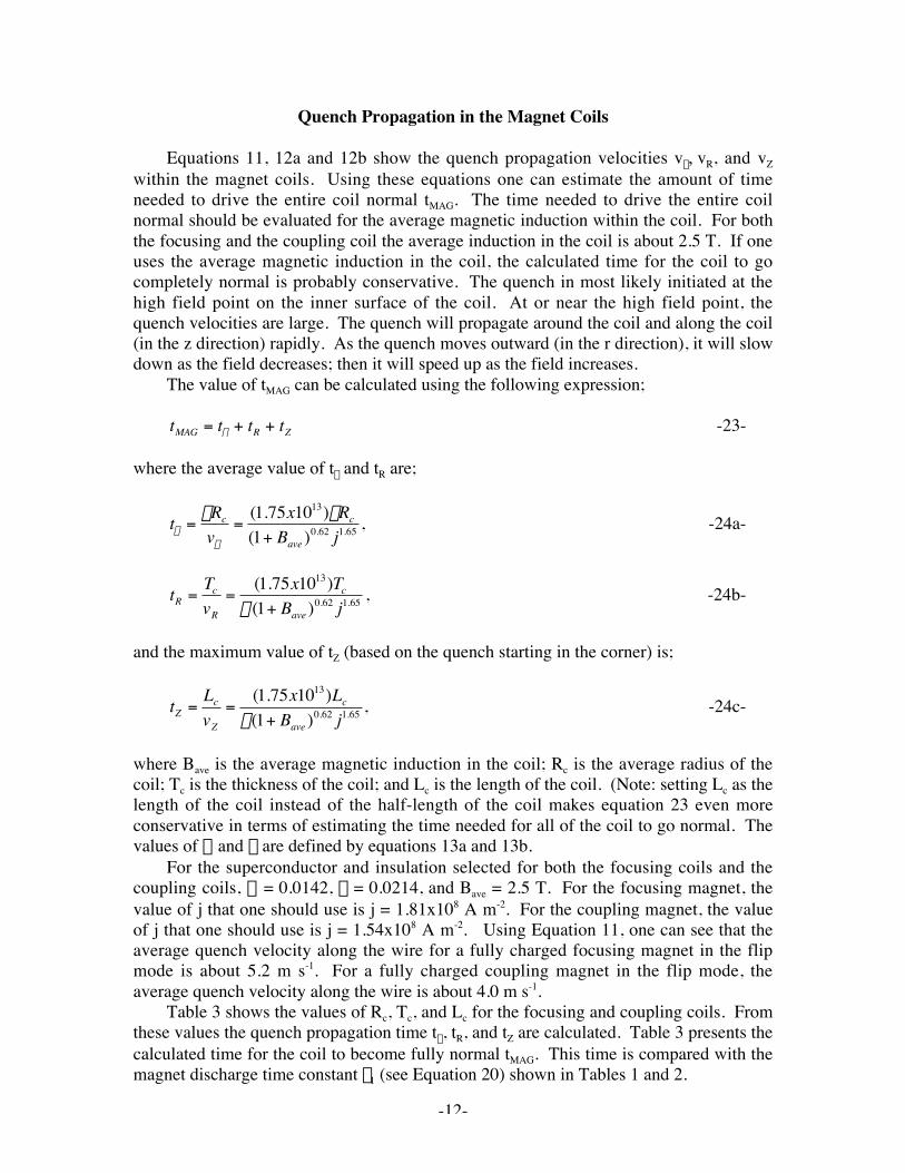
Table 3 shows the values of Rc, Tc, and Lc for the focusing and coupling coils. Fromthese values the quench propagation time tq, tR, and tZ are calculated. Table 3 presents thecalculated time for the coil to become fully normal tMAG. This time is compared with themagnet discharge time constant t1 (see Equation 20) shown in Tables 1 and 2.

-13-

Table 3. Coil Dimensions, and Quench Propagation Times for the Focusing and Coupling coilsThe total quench propagation time within the coils is compared with magnet discharge time constant.

Quench Parameter Focusing CouplingQuench Velocity along the Wire (m s-1) 5.2 4.0Coil Average Half Circumference (m) 0.958 2.45Coil Thickness Tc (m) 0.084 0.116Coil Length Lc (m) 0.210 0.250Time to Propagate Quench around Coil (s) 0.18 0.61Time to Propagate Quench along Tc (s) 1.14 2.04Maximum Time to Propagate Quench along Lc (s) 1.89 2.92Most Probable Time to Quench the Entire Coil (s) 2.27 4.11Maximum Time to Quench the Entire Coil (s) 3.21 5.57Safe Quench Discharge Time Constant (s) 7.33 10.09

Table 3 shows that the calculated most probable time for the quench to propagate toall parts of the focusing coil and coupling coil is less than half of the magnet dischargetime constant for safe quenching. The maximum calculated time for quench propagationwithin the coils is larger, but still safe. Once the whole coil has turned normal, themagnet stored-energy is dumped in the coil.

At an average coil temperature of 100 K, the resistance of a single focusing coil willbe about 41.6 ohms. This resistance is over three times the resistance needed to quenchthe magnet (both coils) safely. The conclusion that one draws from this is that thefocusing magnet will probably quench safely without an external quench protectionsystem even if only one of the two coils turns normal.

At an average coil temperature of 100 K, the resistance of the coupling coil will beabout 173.1 ohms. This resistance is also over three times the resistance needed toquench the magnet safely. The conclusion that one draws from this is that the couplingmagnet will probably quench safely without and external quench protection system.

The high resistance of the coil at or near the end of the quench implies high voltagesduring the quench process. The current is low when the resistance is at its highest, so thevoltages are not as high as one would think. The resistive voltages within the coil will bebalanced by the inductive voltages within the coil. The net voltages to ground or acrossthe magnet layers are in fact quite reasonable. It is always better to quench a magnet allat once, because the voltage buildup within the coil is minimized.

In both magnets, even the most probable calculated quench times are conservative.More of the conductor will be involved early in the quench process than is implied by thequench propagation time calculations. Two other factors come into play. First, the Lc isabout half of what was used in the quench time equation so the time for this part of thequench to take place will be half as much. Second, quench back from the mandrel willgreat speed up the quench propagation process in the coils. Because Quench backspeeds up the quench process within the coil, it also reduces the voltage buildup withinthe coil. If the coils are designed with a layer-to-layer voltage of >500 V and a voltage toground of >3000 V, there should be no trouble during a magnet quench.

Quench back will also have the effect of quenching the second coil in the case of thefocusing magnet. Quench back will permit the three focusing magnets to be hooked inseries and it will also permit the two coupling magnets to be hooked in series.

-14-

Coil Quench Back from the Aluminum Mandrel

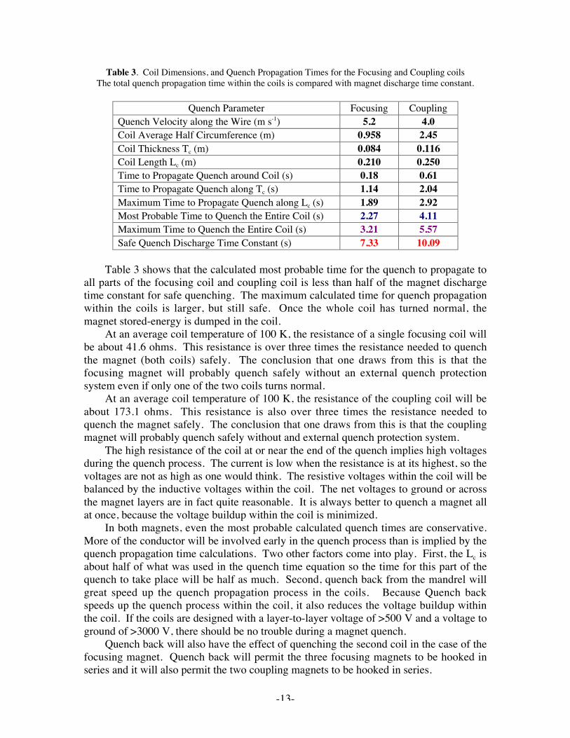
Quench back implies that there is a current flowing in the magnet mandrel during thequench process. The mandrel behaves as a shorted secondary circuit that is inductivelywell coupled with the magnet (the primary circuit). Figure 5 shows the magnet with itscoupled secondary circuit (the mandrel). The only way that a current can flow in themagnet mandrel is that the mandrel is inductively coupled with the magnet coil. In boththe focusing and coupling magnets, the mandrel in a continuous cylinder of aluminumaround the coil package. The coupling between the coils and the adjacent mandrel mustbe reasonably good in order for the current in the magnet to be effectively transferred tothe magnet mandrel.

Figure 5. Quench Protection with a Resistor across the Magnet Leadsand by having a Shorted Secondary Circuit coupled with the Primary Circuit

a) The Effect of the Mandrel as a Shorted Secondary CircuitThe effective coupling coefficient d between the focusing coils and their mandrel is

estimated to be about 0.82. The effective coupling coefficient d between the couplingcoil and its mandrel is estimated to be about 0.92. The use of an effective couplingcoefficient allows one to simplify the quench back problem to a simple circuit. As wewill see later, the region of the mandrel that is closest to the coil will be coupled moreclosely with the than the use of an effective coupling coefficient suggests. This meansthat the quench back times derived from the use of an effective coupling coefficient willbe longer than the actual quench back from the current carrying mandrel to the coil.

A well-coupled low resistance mandrel will affect the quench process in thefollowing ways: 1) A mandrel behaves as a shorted secondary that causes current in thecoil to shift to the mandrel. 2) The mandrel will absorb a substantial amount of themagnet stored-energy during the quench. The mandrel will end up at nearly the sametemperature as the average temperature of the coil at the end of the quench. 3) Since thetime constant for magnetic flux decay is long compared to the time constant for the initialcurrent decay (for a well-coupled system), the transient voltages in the coil are reduced.4) Since a portion of the current in the coil is transferred to the mandrel (for a well-coupled system), the integral of j2dt is reduced, thus the hot spot temperature in the coil is

-15-

reduced. 5) The mandrel heats up from the current flowing within it. This heating causesportions of the coil that are close to the mandrel to turn normal faster than they wouldfrom ordinary quench propagation. This phenomenon is called quench back.

When t1 the coil L over R time constant and t2 the mandrel L over R time constant,respectively, are constant, the current i in the coil has the following relationship;

†

i =i0

t L -t S(t1 -t S )e

- ttL + (t L -t1)

- ttS

È

Î Í Í

˘

˚ ˙ ˙ . -25-

When the coupling is good the coefficient e is small, where e is defined as follows;

†

e = 1-d[ ] = 1-M1-2

2

L1L2

È

Î Í

˘

˚ ˙ -26-

where d is the coupling coefficient between the coil and the mandrel; L1 is the self-inductance of the coil; L2 is the self-inductance of the mandrel; and M1-2 is the mutualinductance between the coil and the mandrel. (Note: for a perfectly coupled coil andmandrel L2 = L1/N1

2 and M1-2 = L1/N1 where N1 is the number of turns in the coil.)With e << 1, tL and tS take the following approximate form;

†

t L ª t1 +t 2 -27a-

and

†

t S ªet1t 2

t1 +t 2. -27b-

When t1 and t2 are constant, the value of F*(TM) takes the following approximateform (with no quench back assumed);

†

F * (TM ) =r +1

rj0

2 t12

2(t1 +t 2)+

t S

2È

Î Í

˘

˚ ˙ . -28-

When on compares equation 28 with equation 18, it is clear that the value of F*(TM) isalways lower when there are a conductive mandrel. When the time constant for themandrel t2 is long compared to the coil circuit time constant t1, the reduction in F*(TM) isquite large, even without quench back to the coil contributing to an additional reductionin the value of t1. The comparison between equations 28 and 18 explains how dramaticreductions in F* are achievable within closely coupled large thin solenoids [10].

Within the MICE coupling and focusing solenoids t2 < t1 (particularly early in thequench) because the mandrel is fabricated from a very high resistivity 6061-T6 aluminum(r = 1.42x10-8 Wm for RRR = 1.8). The MICE focusing magnet has a t2 = 0.43 s. TheMICE coupling magnet has a t2 = 0.40 s. In order for the MICE magnet mandrel tosignificantly reduce F* by itself (without quench back), the mandrel must be made from alow resistivity 1100-O aluminum (r = 8.3x10-10 Wm for RRR = 30). For 1100-Oaluminum t2 for the focusing and coupling mandrels are 7.4 s and 6.8 s respectively.

-16-

In the MICE magnets, F* will not be reduced very much by the mandrel withoutquench back. Quench back from the mandrel to the coil can still be a factor in reducingF* during a quench, even if the mandrel resistivity is high. Quench back become animportant factor for reducing the F* in any coil with a coupled-secondary circuit that isthermally connected to the coil (or coils) [11], [12].

b) Quench Back in the Coil from the MandrelThe process of magnet quench back from a conducting mandrel is adequately

discussed in Reference [9], [11], and [12], so this section of the report will no do muchmore than present the basic equations for the quench back process. In general,importance of quench back to the quench process of the MICE magnets is limited toreducing the hot spot temperature and the voltages that occur within the coil package.The hot spot temperature is reduced because the whole coil becomes fully normal in atime that is less than the time calculated using equation 23. The voltages within the coilare lowered because the resistance of the coil is more evenly spread within the coil.

In order for quench back to be effective in improving the quench process within themagnet, the time for quench back to start tQBS must be substantially less than the time thatthe whole coil would turn normal on its own without quench back tMAG. The question is,“What is substantially shorter time for quench back?” One answer to the question is thattQBS < tMAG – tZ/2. Since tZ is the longest of the three times in equation 23, a much betteranswer is that tQBS < (tq + tR) (See equations 24a and 24b). The authors suggest a shortertime tQBS = (tq + tR)/2.

Once a value for tQBS has been settled on, one can look at the minimum externalresistance Rex in the coil circuit that will induce quench back from the mandrel in the timetQBS. An expression for calculating Rex is given as follows:

†

Rex =L1

t 2

N 2

N1

Ac2

i0

È

Î Í

˘

˚ ˙

DH 2

r2tQBS

È

Î Í Í

˘

˚ ˙ ˙

12

-29-

where L1 is the inductance of the coil; N1 is the number of turns in the coil; and N2 is thenumber of turns in the secondary circuit. (For the magnet mandrel N2 = 1.) Ac2 is thecross-section area of the secondary circuit, and i0 is the starting current in the coil. DH2 isthe change in enthalpy of the material in the secondary circuit needed to induce quenchback. (For the aluminum in the mandrel between 4 K and say 10 K, DH2 = 11700 J m-3.)r2 is the electrical resistivity of the mandrel metal (r2 = 1.42x10-8 W m). t2 can becalculated using the following expression;

†

t 2 =L2

R2ª L1

N 2

N1

Ê

Ë Á

ˆ

¯ ˜

2Ac2

2pRCr2-30-

where RC is the average radius of the coil.From equation 30 one can get an approximate value for Rex, which is given using the

following approximate expression;

-17-

†

Rex =N1

N 2

2pRc

i0

È

Î Í

˘

˚ ˙

r2DH 2

tQBS

È

Î Í Í

˘

˚ ˙ ˙

12

-31-

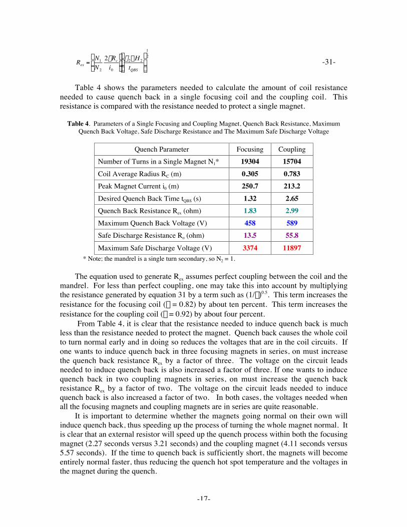
Table 4 shows the parameters needed to calculate the amount of coil resistanceneeded to cause quench back in a single focusing coil and the coupling coil. Thisresistance is compared with the resistance needed to protect a single magnet.

Table 4. Parameters of a Single Focusing and Coupling Magnet, Quench Back Resistance, MaximumQuench Back Voltage, Safe Discharge Resistance and The Maximum Safe Discharge Voltage

Quench Parameter Focusing CouplingNumber of Turns in a Single Magnet N1* 19304 15704Coil Average Radius RC (m) 0.305 0.783Peak Magnet Current i0 (m) 250.7 213.2Desired Quench Back Time tQBS (s) 1.32 2.65Quench Back Resistance Rex (ohm) 1.83 2.99Maximum Quench Back Voltage (V) 458 589Safe Discharge Resistance Ro (ohm) 13.5 55.8Maximum Safe Discharge Voltage (V) 3374 11897

* Note; the mandrel is a single turn secondary, so N2 = 1.

The equation used to generate Rex assumes perfect coupling between the coil and themandrel. For less than perfect coupling, one may take this into account by multiplyingthe resistance generated by equation 31 by a term such as (1/d)0.5. This term increases theresistance for the focusing coil (d = 0.82) by about ten percent. This term increases theresistance for the coupling coil (d = 0.92) by about four percent.

From Table 4, it is clear that the resistance needed to induce quench back is muchless than the resistance needed to protect the magnet. Quench back causes the whole coilto turn normal early and in doing so reduces the voltages that are in the coil circuits. Ifone wants to induce quench back in three focusing magnets in series, on must increasethe quench back resistance Rex by a factor of three. The voltage on the circuit leadsneeded to induce quench back is also increased a factor of three. If one wants to inducequench back in two coupling magnets in series, on must increase the quench backresistance Rex by a factor of two. The voltage on the circuit leads needed to inducequench back is also increased a factor of two. In both cases, the voltages needed whenall the focusing magnets and coupling magnets are in series are quite reasonable.

It is important to determine whether the magnets going normal on their own willinduce quench back, thus speeding up the process of turning the whole magnet normal. Itis clear that an external resistor will speed up the quench process within both the focusingmagnet (2.27 seconds versus 3.21 seconds) and the coupling magnet (4.11 seconds versus5.57 seconds). If the time to quench back is sufficiently short, the magnets will becomeentirely normal faster, thus reducing the quench hot spot temperature and the voltages inthe magnet during the quench.

-18-

In the focusing magnet, the quench within the magnet propagates in threedimensions in time when 0 < t < 0.19 s. The focusing magnet quench is two dimensionalwhen 0.19 < t < 1.14 s. The focusing quench is one dimensional for t > 1.14 s. In thecoupling magnet, the quench propagates in three dimensions in time when 0 < t < 0.61 s.The coupling magnet quench is two dimensional when 0.61 < t < 2.04 s. The couplingquench is one dimensional for t > 2.04 s.

Since the desired quench back time is a little greater than the time where the quenchbecomes one dimensional (1.32 s for the focusing magnet and 2.65 s for the couplingmagnet), one should use the two dimensional scenario for the quench process leading upto quench back within the magnet. If the calculated quench back time based on twodimensional quench propagation is less than the time where the quench process becomesone dimensional, there will be a speed up of the time the coil becomes fully normal. As aresult, both the hot spot temperature and the in coil voltages will be reduced compared tothe cases where there is no quench back from the mandrel to the coil.

The time to the start of quench back tQB can be estimated for a two dimensionalquench if the R direction and the Z direction using the following approximate expression;

†

tQB =tq2

+ 5F2 * L1

L2

R2

R02

N 2

N1

Ac2

abVL2i0

Ê

Ë Á

ˆ

¯ ˜

2È

Î Í Í

˘

˚ ˙ ˙

15

+ tH -32-

where tq is the time to propagate the quench around the coil; L1 is the self-inductance ofthe magnet coil system with N1 turns; and L2 is the self-inductance of the secondarycircuit with N2 turns (N2 = 1 for the MICE magnets). R2 is the resistance of the secondarycircuit; Ac2 is the cross-section area of the secondary winding (the mandrel); VL is thequench propagation velocity along the wire (defined by Equation 11) and i0 is the startingcurrent in the coil (at t = 0). a and b are quench propagation velocity ratios in the R andZ directions respectively that are defined Equations 13a and 13b. tH is the time constantfor the heat to jump from the mandrel across a 1 mm thick plane of ground insulation.(For the MICE magnets tH < 0.01 seconds, so it can be neglected.)

The two-dimensional resistance growth term R02 is defined as follows;

†

R02 =2pRcN1r1

TcLc Ac1

r +1r

-33a-

where r1 is the resistivity of the superconductor matrix material (r1 = 1.55 x 10-10 Wm inour case); a1 is the average radius of the coil; Ac1 is the cross-section area of theconductor (Ac1 = 1.38x10-6 m2 in our case); N1 is the number of turns in the coil; and r isthe copper to superconductor ratio in the coil conductor (r = 4 in our case).

The integral j2dt term for the secondary circuit F2* can be estimated using thefollowing expression for the secondary material at low temperature;

†

F2* = F2 (TQB ) - F2 (4.2) = j20

tQBÚ (t)2 dt =DH 2

r2-33b-

where TQB is the secondary circuit temperature where quench back starts (TQB > 7K); tQBis the time to the start of quench back; and j2(t) is the current density in the secondary as a

-19-

function of time. DH2 is the enthalpy change per unit volume from 4.2 K to TQB, and r2 isthe resistivity of the secondary circuit material over the temperature range from 4.2 K toTQB. (For our case with TQB = 10 K, DH2 = 11700 J m-3, and r2 = 1.42x10-8 Wm.)

One can simplify equation 32 so that tQB is only a function of the material properties,the coil dimensions; the quench propagation velocity along the wire VL; the copper tosuperconductor ratio r and the starting current density j0 in the magnet conductor. Inorder to do this one must define L1, L2 and R2 as follows;

†

L1 ªm0pa1

2N12

l1g1 (a1 ,l1) , -34a-

†

L2 ªm0pa2

2N 22

l 2g2 (a2 ,l 2) , -34b-

and

†

R2 =2pa2r2M N 2

Ac2-34c-

where a1 is the average coil radius (a1 = Rc); a2 is the average secondary circuit radius;

†

l1

is the coil average length (

†

l1 = Lc);

†

l 2 is the secondary circuit average lengths; N1 is thenumber of turns in the coil; and N2 is the number of turns in the secondary circuit. m0 isthe magnetic permeability of vacuum (m0 = 4p x 10-7 Hm-1). g1 is the geometricinductance term for the coil and g2 is the geometric inductance term for the secondarycircuit. Ac2 is the cross-sectional area of the secondary circuit and r2M is the electricalresistivity of the material in that circuit.

If the coils are well coupled, the average radii are nearly the same and the averagelengths are nearly the same so the inductance geometric functions g1 and g2 are the same.Using the well-coupled coil approximation, one can simplify the expression for tQB givenby equation 32 to the following approximate form;

†

tQB =5DH 2r2

r12

Tc2

a 2Lc

2

b 21

VL4 j0

2r

r +1Ê

Ë Á

ˆ

¯ ˜

2È

Î Í Í

˘

˚ ˙ ˙

15

+tq2

-35-

where DH2 is the mandrel enthalpy change needed to induce quench back; r1 is theelectrical resistivity of the matrix material in the conductor. r2 is the electrical resistivityof the mandrel material. (r2 is constant over a wide temperature range.) Tc is thickness ofthe coil; and Lc is the length of the coil. a is defined by equation 13a, and b is defined byequation 13b. The quench velocity along the wire VL is defined by equation 11. j0 is thestarting current density in the conductor cross-section; r is the copper to superconductorratio for the conductor. tq is the time for the quench to propagate the third dimension(half way around the coil).

To be conservative one should use the minimum value of r1 (at say 10 K). It is morerealistic to use a larger value of r1 that represents the average resistivity of the matrix asthe quench develops in the coil. This value may be 3 to 5 times the minimum value of r1.Increasing r1 by a factor of 3 will reduce tQB – tq/2 by about 36 percent.

-20-

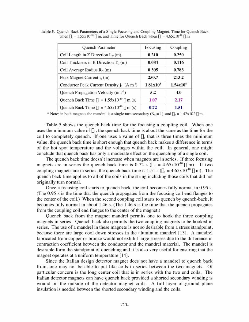
Table 5. Quench Back Parameters of a Single Focusing and Coupling Magnet, Time for Quench Backwhen r1 = 1.55x10-10 Wm, and Time for Quench Back when r1 = 4.65x10-10 Wm

Quench Parameter Focusing CouplingCoil Length in Z Direction LC (m) 0.210 0.250Coil Thickness in R Direction TC (m) 0.084 0.116Coil Average Radius RC (m) 0.305 0.783Peak Magnet Current i0 (m) 250.7 213.2Conductor Peak Current Density j0 (A m-2) 1.81x108 1.54x108

Quench Propagation Velocity (m s-1) 5.2 4.0Quench Back Time r1 = 1.55x10-10 Wm (s) 1.07 2.17Quench Back Time r1 = 4.65x10-10 Wm (s) 0.72 1.51

* Note; in both magnets the mandrel is a single turn secondary (N2 = 1), and r2 = 1.42x10-8 Wm.

Table 5 shows the quench back time for the focusing a coupling coil. When oneuses the minimum value of r1, the quench back time is about the same as the time for thecoil to completely quench. If one uses a value of r1 that is three times the minimumvalue, the quench back time is short enough that quench back makes a difference in termsof the hot spot temperature and the voltages within the coil. In general, one mightconclude that quench back has only a moderate effect on the quenching of a single coil.

The quench back time doesn’t increase when magnets are in series. If three focusingmagnets are in series the quench back time is 0.72 s (r1 = 4.65x10-10 Wm). If twocoupling magnets are in series, the quench back time is 1.51 s (r1 = 4.65x10-10 Wm). Thequench back time applies to all of the coils in the string including those coils that did notoriginally turn normal.

Once a focusing coil starts to quench back, the coil becomes fully normal in 0.95 s.(The 0.95 s is the time that the quench propagates from the focusing coil end flanges tothe center of the coil.) When the second coupling coil starts to quench by quench-back, itbecomes fully normal in about 1.46 s. (The 1.46 s is the time that the quench propagatesfrom the coupling coil end flanges to the center of the magnet.)

Quench back from the magnet mandrel permits one to hook the three couplingmagnets in series. Quench back also permits the two coupling magnets to be hooked inseries. The use of a mandrel in these magnets is not so desirable from a stress standpoint,because there are large cool down stresses in the aluminum mandrel [13]. A mandrelfabricated from copper or bronze would not exhibit large stresses due to the difference incontraction coefficient between the conductor and the mandrel material. The mandrel isdesirable form the standpoint of quenching and it is also very useful for ensuring that themagnet operates at a uniform temperature [14].

Since the Italian design detector magnet does not have a mandrel to quench backfrom, one may not be able to put like coils in series between the two magnets. Ofparticular concern is the long center coil that is in series with the two end coils. TheItalian detector magnets can have quench back provided a shorted secondary winding iswound on the outside of the detector magnet coils. A full layer of ground planeinsulation is needed between the shorted secondary winding and the coils.

-21-

Passive Quenches in the Focusing and Coupling Magnets

Between relatively rapid propagation of the quench in the coils (see Table 3) andquench back induced in the non-quenching coils (see Table 5), it is clear that the focusingcoils and the coupling coils will quench passively, without removing any energy from thecoils. Because the coils quench rapidly, the integral of j2 dt is low enough so that the hotspot temperature at the spot where the quench started is less than 300 K. If the coils areallowed to quench without any external quench protection, all of the magnet stored-energy is shared by all of the coils in the string that are involved in the quench process.

The quench process can be modeled by dividing the quench time into time steps Dt1through DtN. The sum of the time steps Dt1 through DtN is some time like 10 to 15 s (to apoint where the remaining stored magnetic energy is small). At the very minimum, thefirst three time steps should be dictated by the quench process within the magnet (ormagnets). From then on, the remaining time steps can be the same. I suggest thefollowing Dt1 = tq, Dt2 = tQB - tq, and Dt3 = tZ/2. From then on the time steps can be in one-second intervals. If one wants to look at how the quench progresses within the coil, onecan further subdivide steps Dt1, Dt2, and Dt3. (A program called QUENCH, written in thelate 1960s and modified in the mid 1970s subdivides the early time steps to allow on tolook at the quench within the coil. QUENCH does a reasonably good job of modelingquench behavior in magnets despite the fact that the model for quench propagationvelocities within the coil is often incorrect.)

Since the quench progression within the coil is modeled using three time steps, theregions of the coil that are quenching during those time steps should be worked withseparately. For example, a magnet that is in series with the coil quenching does not startto quench until time step 3 when the quench is induced within that magnet throughquench back. For the first three time steps the following resistances can be calculated;

For t = 0

†

l 0 = 0 , and

†

R0 = 0. -36a-

For t = t1

†

l1 =p 3Rc

3abab

, and

†

R1 =r1l1

Ac1

r +1r

, where r1 = 1.55x10-10 Wm. -36b-

For t = t2

†

l 2 = pRcVL

2t22ab

ab. and

†

R2 =r2l 2

Ac1

r +1r

, where r2 = 4.65x10-10 Wm. -36c-

When the quench starts near the end of the coil, divide

†

l1 and

†

l 2 by two.

For t = t3

†

l 3 = pRcNT , and

†

R3 =r3 (Tc1)l 3

Ac1+ (N coil -1) r3 (Tco)l 3

Ac1

È

Î Í

˘

˚ ˙

r +1r

. -36d-

For t = tn

†

l n = 2l 3 for n > 3, and

†

Rn =rn (Tc1)l 3

Ac1+ (N coil -1) rn (Tco)l 3

Ac1

È

Î Í

˘

˚ ˙

r +1r

. -36e-

For the equations above

†

l 0 through

†

l n are the lengths of conductor in the normal state asa function of time. Rc is the average radius of the coil, and NT is the number of turns inthe coil. a is the velocity ratio in the r direction; a is the conductor plus insulationthickness in the r direction; b is the velocity ratio in the z direction; and b is the conductorplus insulation dimension in the z direction. Ac1 is the conductor cross-section area. (InMICE focusing and coupling coils Ac1 = 1.38x10-6 m2.) Ncoil is the number of coils in themagnet string. (For the focusing magnet, Ncoil = 6; for the coupling magnet Ncoil = 2.) Forthe simple model, and for times t3 through tN, the value of r is determined by the averagetemperature of the coil in question. The coil where the quench starts is always hotter.

-22-

The next set of equations are used to calculate the energy in the magnet system E,which has an overall self-inductance LMS. If one knows energy the energy in the magnetat the end of the time step, one can calculate the magnet system current ic at the end of thetime step. It is assumed that none of the magnet stored energy ends up in the mandrel orin external resistors. Given what we know from the Fermilab MUCOOL solenoid,twenty to thirty percent of the magnet stored energy ends up in the mandrel, so thequench analysis presented here is conservative.

For t = 0,

†

E0 =LMS

2i0c

2 . -37a-

LMS is the inductance of the magnet system, and i0 is the starting current for the system.For a single focusing magnet in the flip mode, LMS = 98.6 H. For three focusing magnetsin the flip mode in series, LMS = 295.8 H. For a single focusing magnet in the non-flipmode, LMS = 138.2 H. For three focusing magnets in the non-flip mode hooked in series,LMS = 414.6 H. For a single coupling magnet, LLM = 563 H. For a pair of couplingmagnets in series, LLM = 1126 H.

One can calculate the energy change in magnet circuit as the magnet quenches usingthe equations given below. The equations below assume that the mandrel absorbs verylittle of the energy in the magnet, because t2 << (t1 + t2). The energy change per unit Dtthat leads to a current change in coil can be calculated as follows;

For t = t1,

†

E1 = E0 - DE1 , where

†

DE1 = i0c2 R1

2Dt1. Therefore,

†

i1c =2E1

LMS

È

Î Í

˘

˚ ˙

0.5

. -37b-

For t = t2,

†

E2 = E1 - DE2 , where

†

DE2 = i1c2 R1 + R2

2Dt2. Therefore,

†

i2c =2E2

LMS

È

Î Í

˘

˚ ˙

0.5

. -37c-

For t = t3,

†

E3 = E2 - DE3 , where

†

DE3 = i2c2 R2Dt3. Therefore,

†

i3c =2E3

LMS

È

Î Í

˘

˚ ˙

0.5

. -37d-

For t = tn,

†

En = En-1 - DEn , where

†

DEn = i(n-1)c2 Rn-1Dtn. Therefore,

†

inc =2En

LMS

È

Î Í

˘

˚ ˙

0.5

. -37e-

In the equations above, DEn is the magnet energy change during a time step Dtn; Rn-1 is themagnet system resistance at the start of the time step Dtn; and Rn is the magnet systemresistance at the end of the time step Dtn. One must determine the resistance Rn, which isa function of the average coil temperature Tn, which in turn is a function of the averagethermal energy per unit volume stored in the coil (En/coil volume).

Equations 37b through 37e assume that the mandrel plays no role in the quenchprocess except to cause quench back. In fact, in the MICE magnets, the mandrel canabsorb up thirty percent of the magnet stored-energy at the end of the quench. Thereason that the mandrel is significant is that it is fabricated from a conductive material.The mandrel time constant t2 changes very little during the quench process, because themandrel material resistivity does not change with temperature, when the temperature isless than 120 K. At the end of the quench, t2 can be of the same order as t1, so asignificant portion of the quench energy can end up in the mandrel.

At any time during the quench process the current in the coil and the mandrel canhave the following values;

-23-

†

inC =t1n

t1n +t 2in , where

†

t1n =LMS

Rn and

†

t 2 ªLMS

N coilRM

N 2

N1

Ê

Ë Á

ˆ

¯ ˜

2

, and -38a-

†

inM =t 2

t1n +t 2in

N1

N 2

Ê

Ë Á

ˆ

¯ ˜

2

. R2M is the secondary circuit resistance, where; -38b-

†

R2M =2pRcr2M N 2

Ac2-38c-

The magnet mandrel has is a single turn secondary so N2 = 1.When, t2 is large enough to cause a diversion of the magnet current into the mandrel,

the energy in the magnet circuit En and the coil current inc can be calculated using thefollowing expressions for various values of t;

For t = 0,

†

E0 =LMS

2i0c

2 . -39c-

For t = t1,

†

E1 = E0 - (PC1 - PM1)Dt1;

†

PC1 = i0c2 R1c

2 ;

†

PM1 = 0; and

†

i1c =t11

t11 +t 2

2E1

LMS

È

Î Í

˘

˚ ˙

0.5

. -39b-

For t = t2,

†

E2 = E1 - (PC2 - PM 2)Dt2;

†

PC2 = i1c2 RC1;

†

PM 2 = i1M2 RM ; and

†

i1c =t12

t12 +t 2

2E2

LMS

È

Î Í

˘

˚ ˙

0.5

. -39c-

For t = t3,

†

E3 = E2 - (PC3 - PM 3)Dt3;

†

PC3 = i2c2 RC2;

†

PM 3 = i2M2 RM ; and

†

i3c =t13

t13 +t 2

2E3

LMS

È

Î Í

˘

˚ ˙

0.5

. -39d-

For t = tn,

†

En = En-1 - (PCn - PMn )Dtn ;

†

PCn = i(n-1)c2 Rn-1;

†

PMn = iM (n-1)2 RM ;

†

i1c =t1n

t1n +t 2

2En

LMS

È

Î Í

˘

˚ ˙

0.5

.-39e-

The final equations determine F*(TM). From F*(TM), the hot spot temperature at thepoint where the quench starts TM can be determined;

For t = 0,

†

F0 * (TM ) = 0 . TM = 4.2 K -40a-

For t = t1,

†

F1 * (TM ) = F0 * (TM ) +i0C

2

Ac2 Dt1 . TM can be found in figure 3. -40b-

For t = t2,

†

F2 * (TM ) = F1 * (TM ) +i1C

2

Ac2 Dt2 . TM can be found in figure 3. -40c-

For t = t3,

†

F3 * (TM ) = F2 * (TM ) +i2C

2

Ac2 Dt2 . TM can be found in figure 3. -40d-

For t = tn,

†

Fn * (TM ) = Fn-1 * (TM ) +i(n-1)

2

Ac2 Dtn . TM can be found in figure 3. -40e-

F*(TM) is the integral of j2dt defined by equation 16 where in-1 is the current at t = tn-1 andin is the current at t = tn. Ac is the cross-section area of the matrix.

†

Ac = (Ac1r) (r +1) ,where for both types of magnets Ac1 = 1.38x10-8 m2 and r = 4.

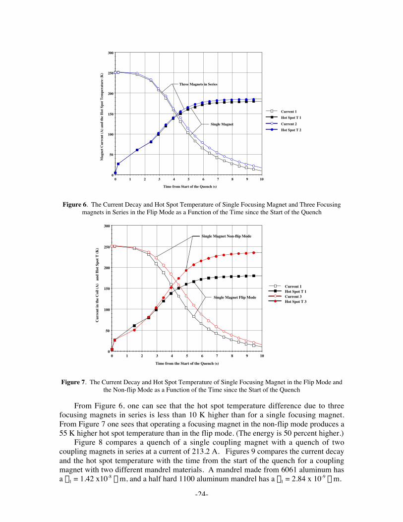
Figure 6 compares a quench of a single focusing magnet with a quench of threefocusing magnets in series. Figure 7 compares a quench of a single focusing magnet inthe flip mode with a quench of a single focusing magnet in the non-flip mode. Both casesin Figure 7 have the same current (250.7 A). Figures 6 and 7 plot the current decay withtime and the hot spot temperature with time. A comparison of Figures 6 and 7 shows thatcurrent flowing in the mandrel causes quench back, which reduces coil current morerapidly, because more of the coil resistance is involved in the quench.

-24-

1098765432100

50

100

150

200

250

300

Current 1Hot Spot T 1Current 2Hot Spot T 2

Time from Start of the Quench (s)

Mag

net C

urre

nt (A

) and

the H

ot S

pot T

empe

ratu

re (K

)

Single Magnet

Three Magnets in Series

Figure 6. The Current Decay and Hot Spot Temperature of Single Focusing Magnet and Three Focusingmagnets in Series in the Flip Mode as a Function of the Time since the Start of the Quench

1098765432100

50

100

150

200

250

300

Current 1Hot Spot T 1Current 3Hot Spot T 3

Time from the Start of the Quench (s)

Cur

rent

in th

e Coi

l (A

) a

nd H

ot S

pot T

(K)

Single Magnet Flip Mode

Single Magnet Non-flip Mode

Figure 7. The Current Decay and Hot Spot Temperature of Single Focusing Magnet in the Flip Mode andthe Non-flip Mode as a Function of the Time since the Start of the Quench

From Figure 6, one can see that the hot spot temperature difference due to threefocusing magnets in series is less than 10 K higher than for a single focusing magnet.From Figure 7 one sees that operating a focusing magnet in the non-flip mode produces a55 K higher hot spot temperature than in the flip mode. (The energy is 50 percent higher.)

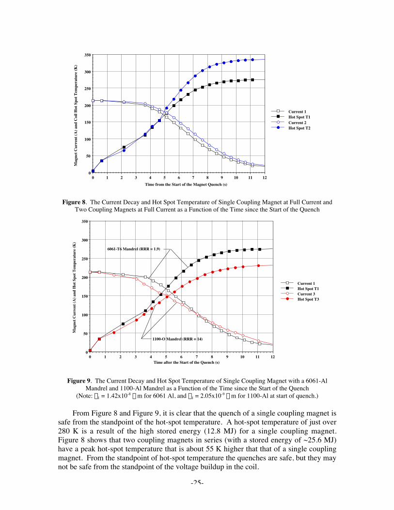
Figure 8 compares a quench of a single coupling magnet with a quench of twocoupling magnets in series at a current of 213.2 A. Figures 9 compares the current decayand the hot spot temperature with the time from the start of the quench for a couplingmagnet with two different mandrel materials. A mandrel made from 6061 aluminum hasa r1 = 1.42 x10-8 Wm, and a half hard 1100 aluminum mandrel has a r1 = 2.84 x 10-9 Wm.

-25-

12111098765432100

50

100

150

200

250

300

350

Current 1Hot Spot T1Current 2Hot Spot T2

Time from the Start of the Magnet Quench (s)

Mag

net C

urre

nt (A

) and

Coi

l Hot

Spo

t Tem

pera

ture

(K)

Figure 8. The Current Decay and Hot Spot Temperature of Single Coupling Magnet at Full Current andTwo Coupling Magnets at Full Current as a Function of the Time since the Start of the Quench

12111098765432100

50

100

150

200

250

300

350

Current 1Hot Spot T1Current 3Hot Spot T3

Time after the Start of the Quench (s)

Mag

net C

urre

nt (A

) and

Hot

Spo

t Tem

pera

ture

(K)

6061-T6 Mandrel (RRR = 1.9)

1100-O Mandrel (RRR = 14)

Figure 9. The Current Decay and Hot Spot Temperature of Single Coupling Magnet with a 6061-AlMandrel and 1100-Al Mandrel as a Function of the Time since the Start of the Quench

(Note: r1 = 1.42x10-8 Wm for 6061 Al, and r1 = 2.05x10-9 Wm for 1100-Al at start of quench.)

From Figure 8 and Figure 9, it is clear that the quench of a single coupling magnet issafe from the standpoint of the hot-spot temperature. A hot-spot temperature of just over280 K is a result of the high stored energy (12.8 MJ) for a single coupling magnet.Figure 8 shows that two coupling magnets in series (with a stored energy of ~25.6 MJ)have a peak hot-spot temperature that is about 55 K higher that that of a single couplingmagnet. From the standpoint of hot-spot temperature the quenches are safe, but they maynot be safe from the standpoint of the voltage buildup in the coil.

-26-

Figure 9 shows the effect of slowing the quench process down by using a moreconductive mandrel. A half hard 1100 aluminum mandrel has an electrical resistivity thatis a factor of seven lower than a 6061 aluminum mandrel at temperatures below 40 K[15]. Above 60 K, the 1100-aluminum mandrel resistivity will be higher, but not as highas the 6061-aluminum mandrel resistivity. At temperatures below 40 K, the mandrelcurrent decay time constant will be about 2.8 seconds. The use of a low-resistivitymandrel appears to reduce the hot spot temperature by 35 to 40 K. One reason for this isthat much of the F* gain occurs before the coil has gone completely normal due toquench back. The other reason is that the mandrel takes current away from the magnetcoil.

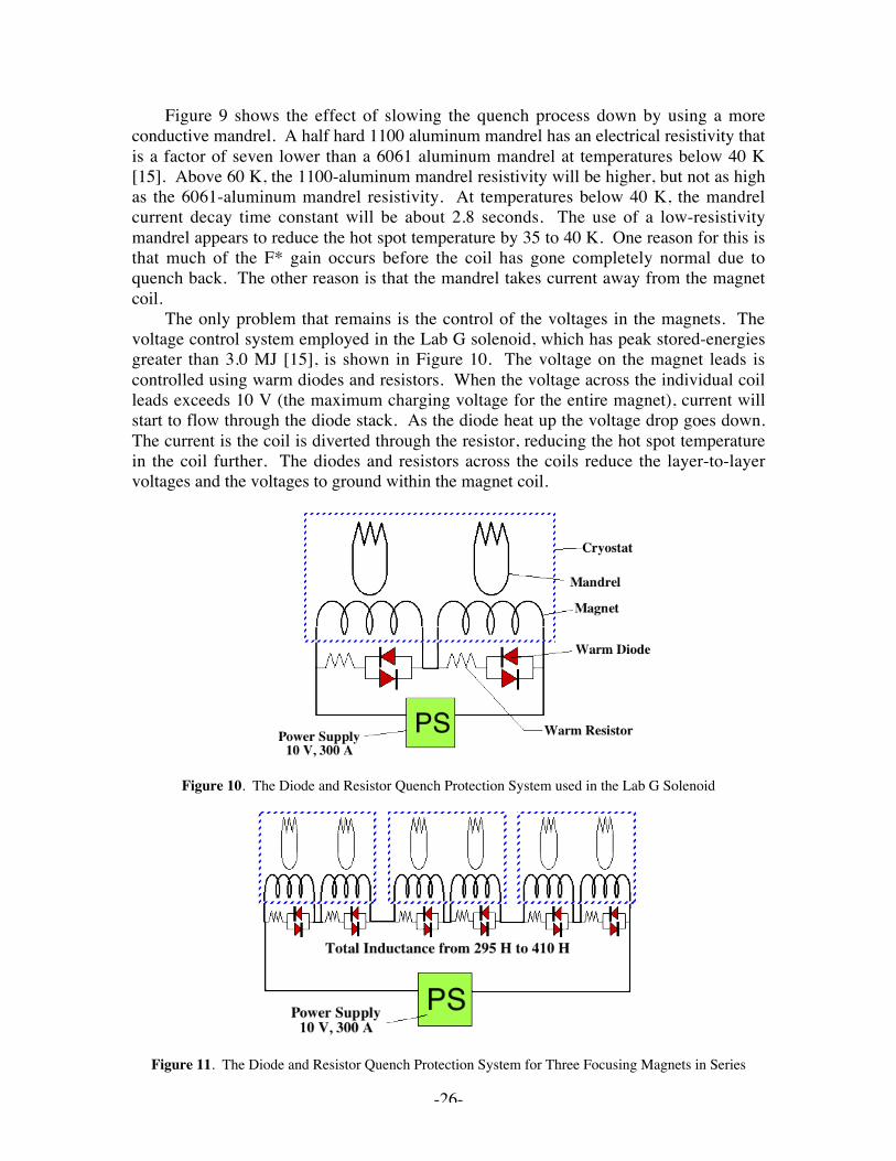
The only problem that remains is the control of the voltages in the magnets. Thevoltage control system employed in the Lab G solenoid, which has peak stored-energiesgreater than 3.0 MJ [15], is shown in Figure 10. The voltage on the magnet leads iscontrolled using warm diodes and resistors. When the voltage across the individual coilleads exceeds 10 V (the maximum charging voltage for the entire magnet), current willstart to flow through the diode stack. As the diode heat up the voltage drop goes down.The current is the coil is diverted through the resistor, reducing the hot spot temperaturein the coil further. The diodes and resistors across the coils reduce the layer-to-layervoltages and the voltages to ground within the magnet coil.

Figure 10. The Diode and Resistor Quench Protection System used in the Lab G Solenoid

Figure 11. The Diode and Resistor Quench Protection System for Three Focusing Magnets in Series

-27-

Figure 11 shows the quench protections system for three focusing magnets hookedup in series. The quench protection system shown in Figure 11 should have the sameperformance as the quench protection system shown in Figure 10. We know that thequench protections system shown in Figure 10 works very well, so the authors don’texpect the three focusing magnets in series to behave much different from the Lab Gmagnet. The previous statement is likely to be accurate up to a stored energy per magnetof about 3 MJ. The peak current in the focusing magnets for the low beta cases in thenon-flip mode may result in magnet stored energies greater than 3.0 MJ. This mayrequire that the non-flip low beta cases be operated at an average momentum of less than200 MeV/c, just as for many of the flip cases.

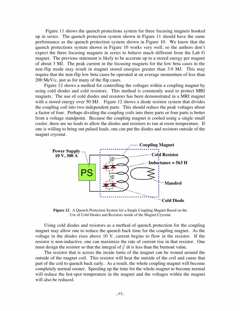
Figure 12 shows a method for controlling the voltages within a coupling magnet byusing cold diodes and cold resistors. This method is commonly used to protect MRImagnets. The use of cold diodes and resistors has been demonstrated in a MRI magnetwith a stored energy over 50 MJ. Figure 12 shows a diode resistor system that dividesthe coupling coil into two independent parts. This should reduce the peak voltages abouta factor of four. Perhaps dividing the coupling coils into three parts or four parts is betterfrom a voltage standpoint. Because the coupling magnet is cooled using a single smallcooler, there are no leads to allow the diodes and resistors to run at room temperature. Ifone is willing to bring out pulsed leads, one can put the diodes and resistors outside of themagnet cryostat.

Figure 12. A Quench Protection System for a Single Coupling Magnet Based on theUse of Cold Diodes and Resistors inside of the Magnet Cryostat

Using cold diodes and resistors as a method of quench protection for the couplingmagnet may allow one to reduce the quench back time for the coupling magnet. As thevoltage in the diodes rises above 10 V, current begins to flow in the resistor. If theresistor is non-inductive, one can maximize the rate of current rise in that resistor. Onemust design the resistor so that the integral of j2 dt is less than the burnout value.

The resistor that is across the inside turns of the magnet can be wound around theoutside of the magnet coil. This resistor will heat the outside of the coil and cause thatpart of the coil to quench back early. As a result, the whole coupling magnet will becomecompletely normal sooner. Speeding up the time for the whole magnet to become normalwill reduce the hot-spot temperature in the magnet and the voltages within the magnetwill also be reduced.

-28-

Magnetic Coupling between Various Magnets in MICE

The power supply for the MICE magnets is determined by three factors. They are;1) the required charge time for the magnet set, 2) the voltages generated by the chargingof a nearby magnet, and 3) the total current change in a coil caused by the quenching of anearby magnet or set of magnets. In addition, when a nearby superconducting magnetquenches, coupling from the quenching magnet to a second magnet mandrel may heat thesecond magnet mandrel enough to induce quench back in the second magnet. Thiscoupling between a magnet and an adjacent magnet mandrel and quench back heatingthat results will be dealt with in a later section of this report.

The hook up of the magnets in the MICE cooling channel is quite clear. It has beenproposed that the three focusing coils be hooked up in series so that they can be run froma single power supply. It has also been proposed that the two coupling coil can behooked up in series and run from a single power supply. From the quench simulations itis clear that the coupling magnets can be hooked together in series. The question iswhether the two coupling magnet should be hooked together in series. This section willlook at the magnetic coupling for both alternatives.

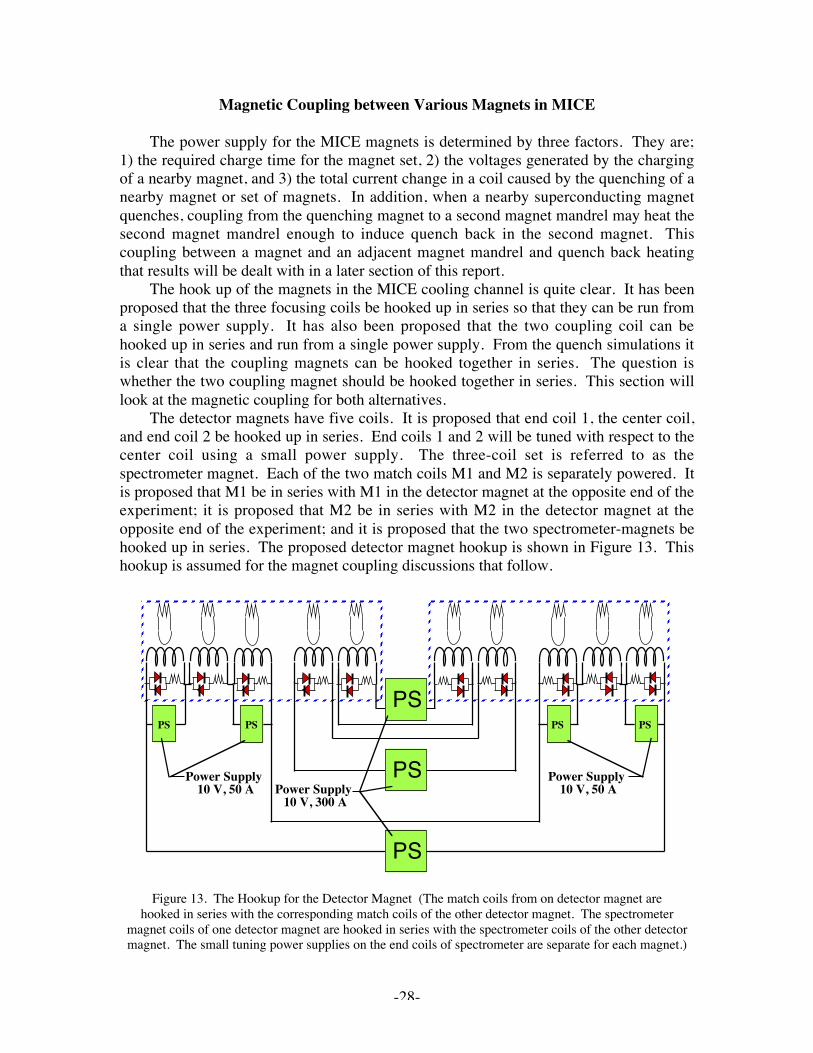
The detector magnets have five coils. It is proposed that end coil 1, the center coil,and end coil 2 be hooked up in series. End coils 1 and 2 will be tuned with respect to thecenter coil using a small power supply. The three-coil set is referred to as thespectrometer magnet. Each of the two match coils M1 and M2 is separately powered. Itis proposed that M1 be in series with M1 in the detector magnet at the opposite end of theexperiment; it is proposed that M2 be in series with M2 in the detector magnet at theopposite end of the experiment; and it is proposed that the two spectrometer-magnets behooked up in series. The proposed detector magnet hookup is shown in Figure 13. Thishookup is assumed for the magnet coupling discussions that follow.

Power Supply10 V, 300 A

Power Supply10 V, 50 A

PS PSPSPS

PS

PS

PS

Power Supply10 V, 50 A

Figure 13. The Hookup for the Detector Magnet (The match coils from on detector magnet arehooked in series with the corresponding match coils of the other detector magnet. The spectrometer

magnet coils of one detector magnet are hooked in series with the spectrometer coils of the other detectormagnet. The small tuning power supplies on the end coils of spectrometer are separate for each magnet.)

-29-

a) Inductance calculationsFor calculating the inductance matrix, an analytic approach was chosen [17]; the

results were verified using finite element software (FEA). The self-inductance of a loopof wire with the radius R and circular cross section with radius ra is:

˜̃¯

ˆÁÁË

Ê-=

478

ln0a

self rR

RL m . -44-

For wires with a rectangular cross-section of height h and width w, the followingapproximation gives good results:

phw

ra

⋅= . -45-

The mutual inductance between two current loops of radius R1 and R2 is calculatedusing;

˙̊˘

ÍÎ

È --= )(2

)()2

(210 kEk

kKkk

RRLab m -46-

where E(k) and K(k) are elliptic integrals, defined as

Ú -=2/

0

22 sin1)(p

ff dkkE -46a-

Ú-

=2/

0 22 sin1)(

p

f

f

k

dkK -46b-

where k is a geometry factor, defined by the radii of the current loops R and the distancez between them:

2221

21

z + )R + (RR R 4

=k . -46c-

A program was written to calculate the inductance matrix for each coil with respect tothe others. The inductance of a single coil is the sum of all self-inductances and allmutual inductances of the individual turns (labelled k) with all the others (labelled l):

ÂÂ=N

kl

N

ooil LL11

. -47-

The same method can be employed for calculating the mutual inductances between coils.For verifying the obtained results, FEA was used. In general, the inductance of a

single coil can be obtained easily if the magnetic energy Wmag and current I in theconductor is known:

-30-

2

21

ILW coilmag= . -48-

Solving the above equation for Lcoil yields

2

2

I

WL mag

coil

⋅= . -49-

The magnetic energy can be obtained easily by an FEA simulation, integrating thefollowing expression over the complete model volume V:

Ú⋅

= dVHB

Wmag 2-50-

For obtaining the mutual inductance between two coils, it is necessary to do twosimulations: in the first simulation both coils are powered in the same direction, and inthe second simulation the current in one coil is reversed. The inductances Lea and Leb forboth arrangements is obtained using the above equations; the mutual inductance Lab canbe calculated by [18];

4ebea

ab

LLL

-= -51-

Selected values of the mutual inductance and self-inductance were verified using thisapproach. It was found that the analytic code is in good agreement with the finiteelement results (of the order of 1-2 percent).

b) Calculation of Inductance Networks for the MICE Magnet SystemTables 6 and 7 show the inductance network for the MICE magnets with the

coupling coils in series in the full flip and full non-flip modes. Intermediate mixed flipand non-flip cases are not included in the analysis. All of the information that isnecessary to know about the inductive behavior of the magnets and the resultant couplingcan be learned from studying the two extreme cases (and most likely operating cases).The diagonal between the upper left hand corner and the lower right hand corner ofTables 6 and 7 is the self-inductance of the magnet systems in question. The off diagonalterms are the mutual inductance terms between magnet systems.

Tables 8 and 9 show the inductance network for the MICE magnets with thecoupling coils separately powered in the full flip and full non-flip modes. Intermediatemixed flip and non-flip cases are not included in the analysis. All of the information thatis necessary to know about the inductive behavior of the magnets can be learned from theextreme cases. The diagonal between the upper left hand corner and the lower right handcorner of Tables 8 and 9 is the self-inductance of the magnet system in question. The offdiagonal terms are the mutual inductance terms between magnet systems.

-31-

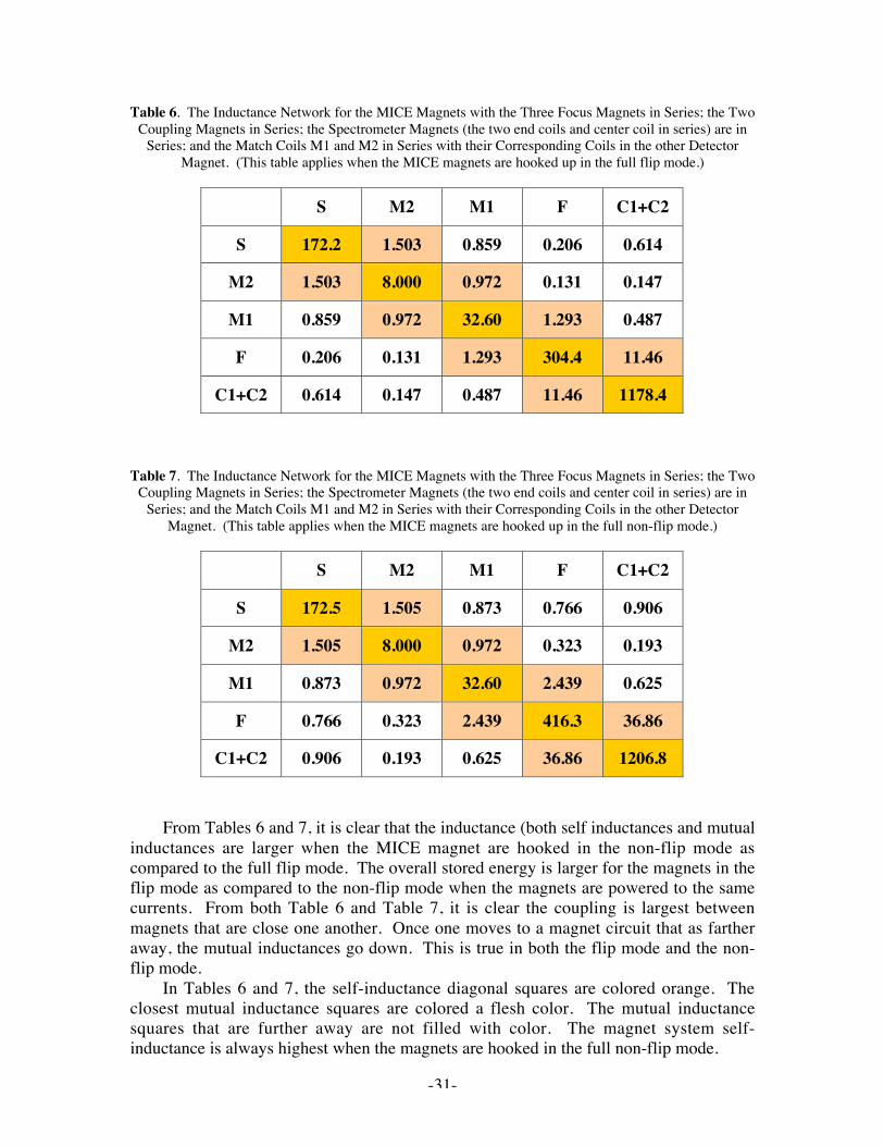
Table 6. The Inductance Network for the MICE Magnets with the Three Focus Magnets in Series; the TwoCoupling Magnets in Series; the Spectrometer Magnets (the two end coils and center coil in series) are in

Series; and the Match Coils M1 and M2 in Series with their Corresponding Coils in the other DetectorMagnet. (This table applies when the MICE magnets are hooked up in the full flip mode.)

S M2 M1 F C1+C2

S 172.2 1.503 0.859 0.206 0.614

M2 1.503 8.000 0.972 0.131 0.147

M1 0.859 0.972 32.60 1.293 0.487

F 0.206 0.131 1.293 304.4 11.46

C1+C2 0.614 0.147 0.487 11.46 1178.4

Table 7. The Inductance Network for the MICE Magnets with the Three Focus Magnets in Series; the TwoCoupling Magnets in Series; the Spectrometer Magnets (the two end coils and center coil in series) are in

Series; and the Match Coils M1 and M2 in Series with their Corresponding Coils in the other DetectorMagnet. (This table applies when the MICE magnets are hooked up in the full non-flip mode.)

S M2 M1 F C1+C2

S 172.5 1.505 0.873 0.766 0.906

M2 1.505 8.000 0.972 0.323 0.193

M1 0.873 0.972 32.60 2.439 0.625

F 0.766 0.323 2.439 416.3 36.86

C1+C2 0.906 0.193 0.625 36.86 1206.8

From Tables 6 and 7, it is clear that the inductance (both self inductances and mutualinductances are larger when the MICE magnet are hooked in the non-flip mode ascompared to the full flip mode. The overall stored energy is larger for the magnets in theflip mode as compared to the non-flip mode when the magnets are powered to the samecurrents. From both Table 6 and Table 7, it is clear the coupling is largest betweenmagnets that are close one another. Once one moves to a magnet circuit that as fartheraway, the mutual inductances go down. This is true in both the flip mode and the non-flip mode.

In Tables 6 and 7, the self-inductance diagonal squares are colored orange. Theclosest mutual inductance squares are colored a flesh color. The mutual inductancesquares that are further away are not filled with color. The magnet system self-inductance is always highest when the magnets are hooked in the full non-flip mode.

-32-

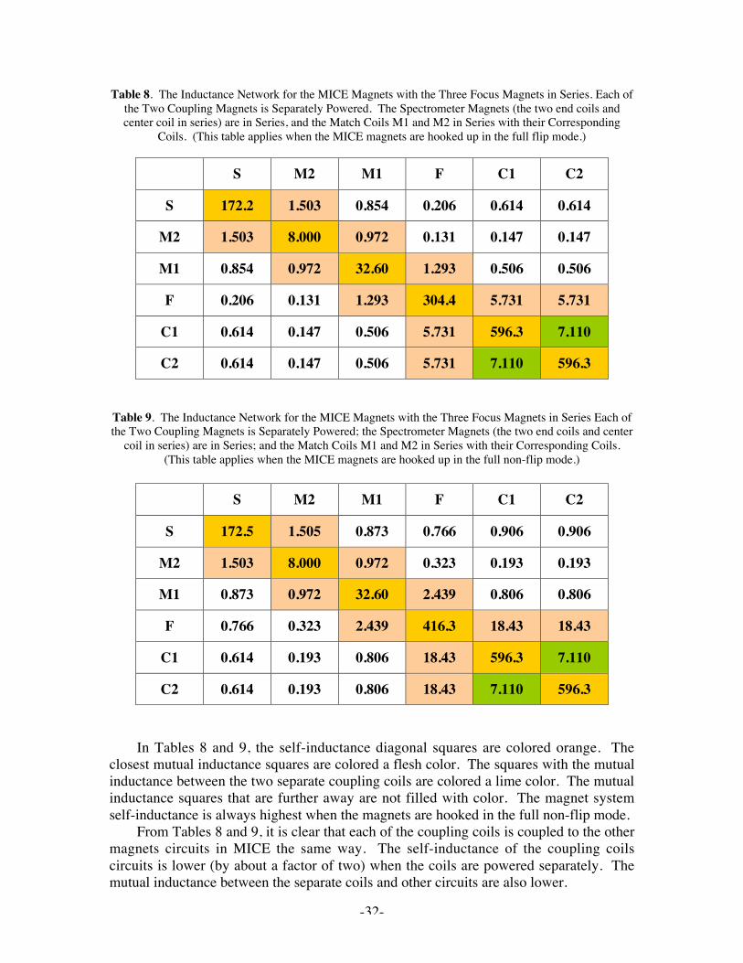
Table 8. The Inductance Network for the MICE Magnets with the Three Focus Magnets in Series. Each ofthe Two Coupling Magnets is Separately Powered. The Spectrometer Magnets (the two end coils andcenter coil in series) are in Series, and the Match Coils M1 and M2 in Series with their Corresponding

Coils. (This table applies when the MICE magnets are hooked up in the full flip mode.)

S M2 M1 F C1 C2

S 172.2 1.503 0.854 0.206 0.614 0.614

M2 1.503 8.000 0.972 0.131 0.147 0.147

M1 0.854 0.972 32.60 1.293 0.506 0.506

F 0.206 0.131 1.293 304.4 5.731 5.731

C1 0.614 0.147 0.506 5.731 596.3 7.110

C2 0.614 0.147 0.506 5.731 7.110 596.3

Table 9. The Inductance Network for the MICE Magnets with the Three Focus Magnets in Series Each ofthe Two Coupling Magnets is Separately Powered; the Spectrometer Magnets (the two end coils and center

coil in series) are in Series; and the Match Coils M1 and M2 in Series with their Corresponding Coils.(This table applies when the MICE magnets are hooked up in the full non-flip mode.)

S M2 M1 F C1 C2

S 172.5 1.505 0.873 0.766 0.906 0.906

M2 1.503 8.000 0.972 0.323 0.193 0.193

M1 0.873 0.972 32.60 2.439 0.806 0.806

F 0.766 0.323 2.439 416.3 18.43 18.43

C1 0.614 0.193 0.806 18.43 596.3 7.110

C2 0.614 0.193 0.806 18.43 7.110 596.3

In Tables 8 and 9, the self-inductance diagonal squares are colored orange. Theclosest mutual inductance squares are colored a flesh color. The squares with the mutualinductance between the two separate coupling coils are colored a lime color. The mutualinductance squares that are further away are not filled with color. The magnet systemself-inductance is always highest when the magnets are hooked in the full non-flip mode.

From Tables 8 and 9, it is clear that each of the coupling coils is coupled to the othermagnets circuits in MICE the same way. The self-inductance of the coupling coilscircuits is lower (by about a factor of two) when the coils are powered separately. Themutual inductance between the separate coils and other circuits are also lower.

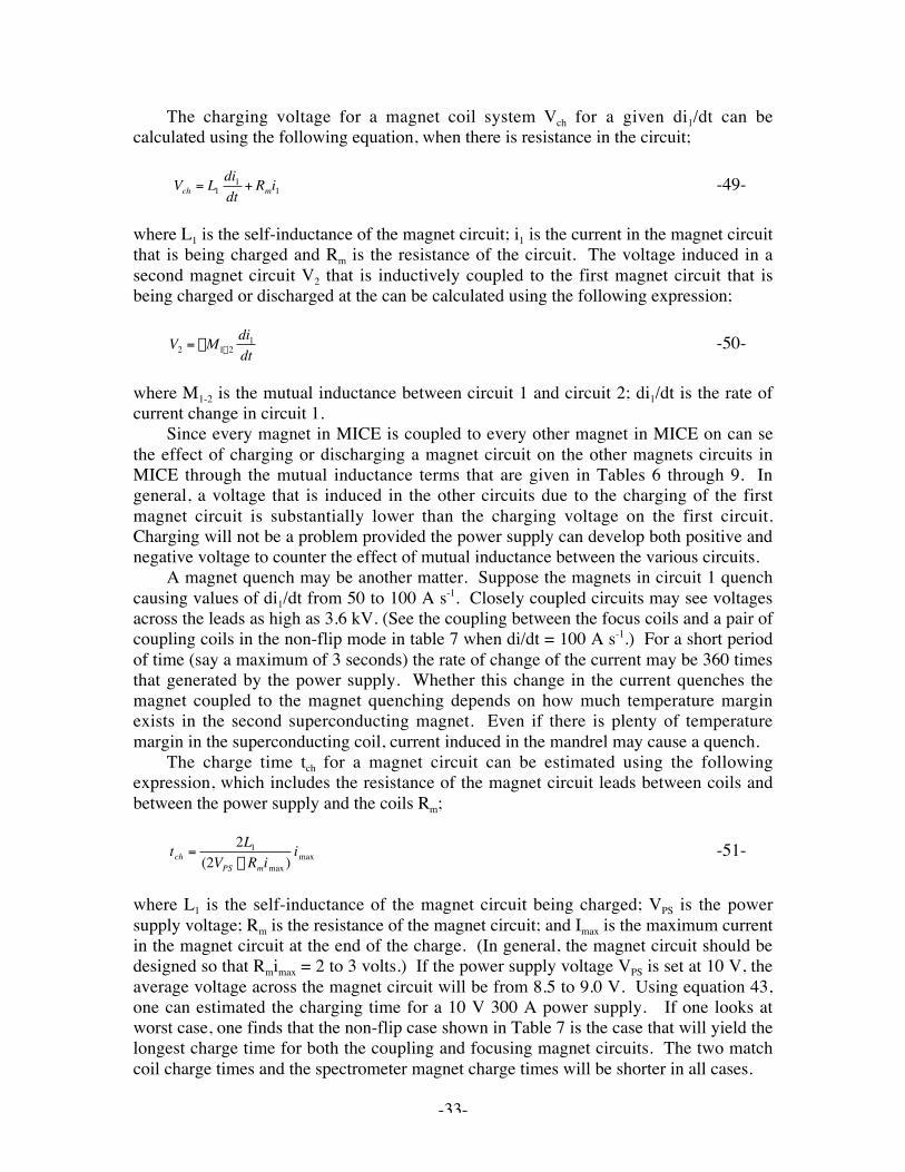
-33-

The charging voltage for a magnet coil system Vch for a given di1/dt can becalculated using the following equation, when there is resistance in the circuit;

†

Vch = L1di1dt

+ Rmi1 -49-

where L1 is the self-inductance of the magnet circuit; i1 is the current in the magnet circuitthat is being charged and Rm is the resistance of the circuit. The voltage induced in asecond magnet circuit V2 that is inductively coupled to the first magnet circuit that isbeing charged or discharged at the can be calculated using the following expression;

†

V2 = -M1-2di1dt

-50-

where M1-2 is the mutual inductance between circuit 1 and circuit 2; di1/dt is the rate ofcurrent change in circuit 1.

Since every magnet in MICE is coupled to every other magnet in MICE on can sethe effect of charging or discharging a magnet circuit on the other magnets circuits inMICE through the mutual inductance terms that are given in Tables 6 through 9. Ingeneral, a voltage that is induced in the other circuits due to the charging of the firstmagnet circuit is substantially lower than the charging voltage on the first circuit.Charging will not be a problem provided the power supply can develop both positive andnegative voltage to counter the effect of mutual inductance between the various circuits.

A magnet quench may be another matter. Suppose the magnets in circuit 1 quenchcausing values of di1/dt from 50 to 100 A s-1. Closely coupled circuits may see voltagesacross the leads as high as 3.6 kV. (See the coupling between the focus coils and a pair ofcoupling coils in the non-flip mode in table 7 when di/dt = 100 A s-1.) For a short periodof time (say a maximum of 3 seconds) the rate of change of the current may be 360 timesthat generated by the power supply. Whether this change in the current quenches themagnet coupled to the magnet quenching depends on how much temperature marginexists in the second superconducting magnet. Even if there is plenty of temperaturemargin in the superconducting coil, current induced in the mandrel may cause a quench.

The charge time tch for a magnet circuit can be estimated using the followingexpression, which includes the resistance of the magnet circuit leads between coils andbetween the power supply and the coils Rm;

†

tch =2L1

(2VPS - Rmimax )imax -51-

where L1 is the self-inductance of the magnet circuit being charged; VPS is the powersupply voltage; Rm is the resistance of the magnet circuit; and Imax is the maximum currentin the magnet circuit at the end of the charge. (In general, the magnet circuit should bedesigned so that Rmimax = 2 to 3 volts.) If the power supply voltage VPS is set at 10 V, theaverage voltage across the magnet circuit will be from 8.5 to 9.0 V. Using equation 43,one can estimated the charging time for a 10 V 300 A power supply. If one looks atworst case, one finds that the non-flip case shown in Table 7 is the case that will yield thelongest charge time for both the coupling and focusing magnet circuits. The two matchcoil charge times and the spectrometer magnet charge times will be shorter in all cases.

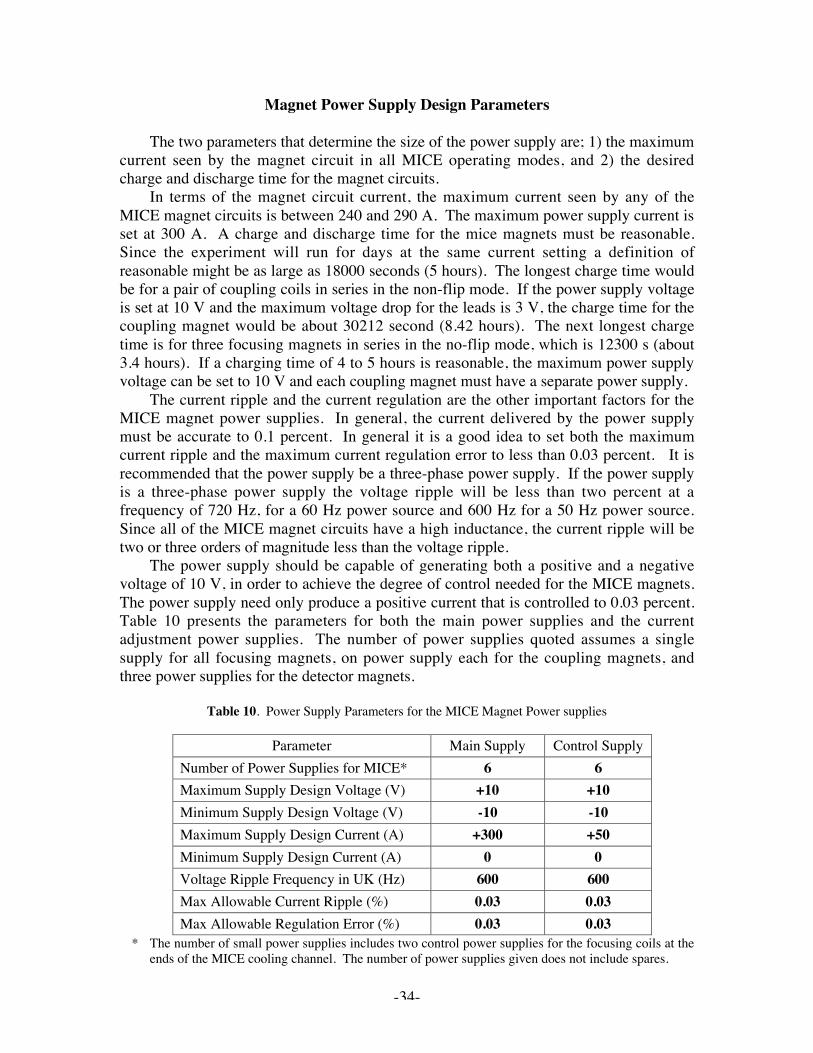
-34-

Magnet Power Supply Design Parameters

The two parameters that determine the size of the power supply are; 1) the maximumcurrent seen by the magnet circuit in all MICE operating modes, and 2) the desiredcharge and discharge time for the magnet circuits.

In terms of the magnet circuit current, the maximum current seen by any of theMICE magnet circuits is between 240 and 290 A. The maximum power supply current isset at 300 A. A charge and discharge time for the mice magnets must be reasonable.Since the experiment will run for days at the same current setting a definition ofreasonable might be as large as 18000 seconds (5 hours). The longest charge time wouldbe for a pair of coupling coils in series in the non-flip mode. If the power supply voltageis set at 10 V and the maximum voltage drop for the leads is 3 V, the charge time for thecoupling magnet would be about 30212 second (8.42 hours). The next longest chargetime is for three focusing magnets in series in the no-flip mode, which is 12300 s (about3.4 hours). If a charging time of 4 to 5 hours is reasonable, the maximum power supplyvoltage can be set to 10 V and each coupling magnet must have a separate power supply.

The current ripple and the current regulation are the other important factors for theMICE magnet power supplies. In general, the current delivered by the power supplymust be accurate to 0.1 percent. In general it is a good idea to set both the maximumcurrent ripple and the maximum current regulation error to less than 0.03 percent. It isrecommended that the power supply be a three-phase power supply. If the power supplyis a three-phase power supply the voltage ripple will be less than two percent at afrequency of 720 Hz, for a 60 Hz power source and 600 Hz for a 50 Hz power source.Since all of the MICE magnet circuits have a high inductance, the current ripple will betwo or three orders of magnitude less than the voltage ripple.

The power supply should be capable of generating both a positive and a negativevoltage of 10 V, in order to achieve the degree of control needed for the MICE magnets.The power supply need only produce a positive current that is controlled to 0.03 percent.Table 10 presents the parameters for both the main power supplies and the currentadjustment power supplies. The number of power supplies quoted assumes a singlesupply for all focusing magnets, on power supply each for the coupling magnets, andthree power supplies for the detector magnets.

Table 10. Power Supply Parameters for the MICE Magnet Power supplies

Parameter Main Supply Control SupplyNumber of Power Supplies for MICE* 6 6Maximum Supply Design Voltage (V) +10 +10Minimum Supply Design Voltage (V) -10 -10Maximum Supply Design Current (A) +300 +50Minimum Supply Design Current (A) 0 0Voltage Ripple Frequency in UK (Hz) 600 600Max Allowable Current Ripple (%) 0.03 0.03Max Allowable Regulation Error (%) 0.03 0.03

* The number of small power supplies includes two control power supplies for the focusing coils at theends of the MICE cooling channel. The number of power supplies given does not include spares.

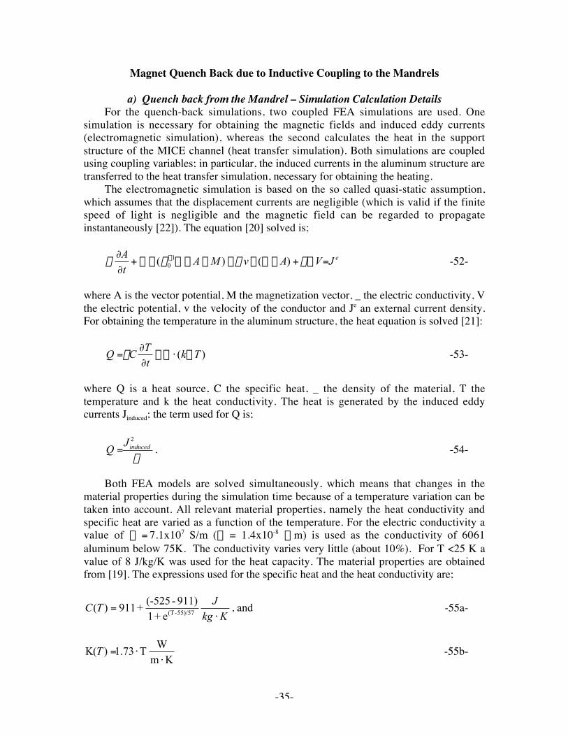
-35-

Magnet Quench Back due to Inductive Coupling to the Mandrels

a) Quench back from the Mandrel – Simulation Calculation DetailsFor the quench-back simulations, two coupled FEA simulations are used. One

simulation is necessary for obtaining the magnetic fields and induced eddy currents(electromagnetic simulation), whereas the second calculates the heat in the supportstructure of the MICE channel (heat transfer simulation). Both simulations are coupledusing coupling variables; in particular, the induced currents in the aluminum structure aretransferred to the heat transfer simulation, necessary for obtaining the heating.

The electromagnetic simulation is based on the so called quasi-static assumption,which assumes that the displacement currents are negligible (which is valid if the finitespeed of light is negligible and the magnetic field can be regarded to propagateinstantaneously [22]). The equation [20] solved is;

eJVAvMAtA

=—+¥—¥--¥—¥—+∂∂ - ssms )()( 1

0 -52-

where A is the vector potential, M the magnetization vector, _ the electric conductivity, Vthe electric potential, v the velocity of the conductor and Je an external current density.For obtaining the temperature in the aluminum structure, the heat equation is solved [21]:

)( TktT

CQ —⋅—-∂∂

=r -53-

where Q is a heat source, C the specific heat, _ the density of the material, T thetemperature and k the heat conductivity. The heat is generated by the induced eddycurrents Jinduced; the term used for Q is;

s

2inducedJ

Q = . -54-

Both FEA models are solved simultaneously, which means that changes in thematerial properties during the simulation time because of a temperature variation can betaken into account. All relevant material properties, namely the heat conductivity andspecific heat are varied as a function of the temperature. For the electric conductivity avalue of s = 7.1x107 S/m (r = 1.4x10-8 Wm) is used as the conductivity of 6061aluminum below 75K. The conductivity varies very little (about 10%). For T <25 K avalue of 8 J/kg/K was used for the heat capacity. The material properties are obtainedfrom [19]. The expressions used for the specific heat and the heat conductivity are;

KkgJ

TC⋅

= 55)/57-(Te+1911)-(-525

+911)( , and -55a-

KmW

T1.73)(K⋅

⋅=T -55b-

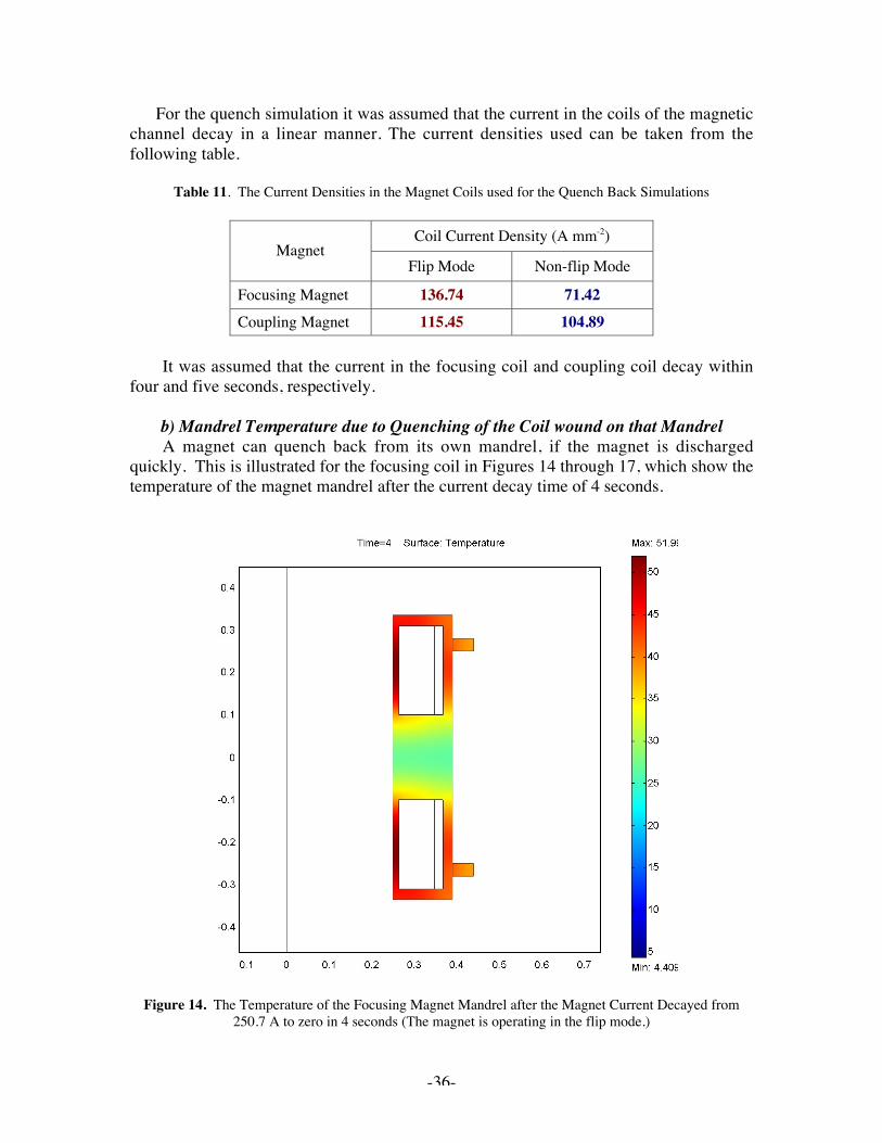
-36-

For the quench simulation it was assumed that the current in the coils of the magneticchannel decay in a linear manner. The current densities used can be taken from thefollowing table.

Table 11. The Current Densities in the Magnet Coils used for the Quench Back Simulations

Coil Current Density (A mm-2)Magnet

Flip Mode Non-flip Mode

Focusing Magnet 136.74 71.42Coupling Magnet 115.45 104.89

It was assumed that the current in the focusing coil and coupling coil decay withinfour and five seconds, respectively.

b) Mandrel Temperature due to Quenching of the Coil wound on that MandrelA magnet can quench back from its own mandrel, if the magnet is discharged

quickly. This is illustrated for the focusing coil in Figures 14 through 17, which show thetemperature of the magnet mandrel after the current decay time of 4 seconds.

Figure 14. The Temperature of the Focusing Magnet Mandrel after the Magnet Current Decayed from250.7 A to zero in 4 seconds (The magnet is operating in the flip mode.)

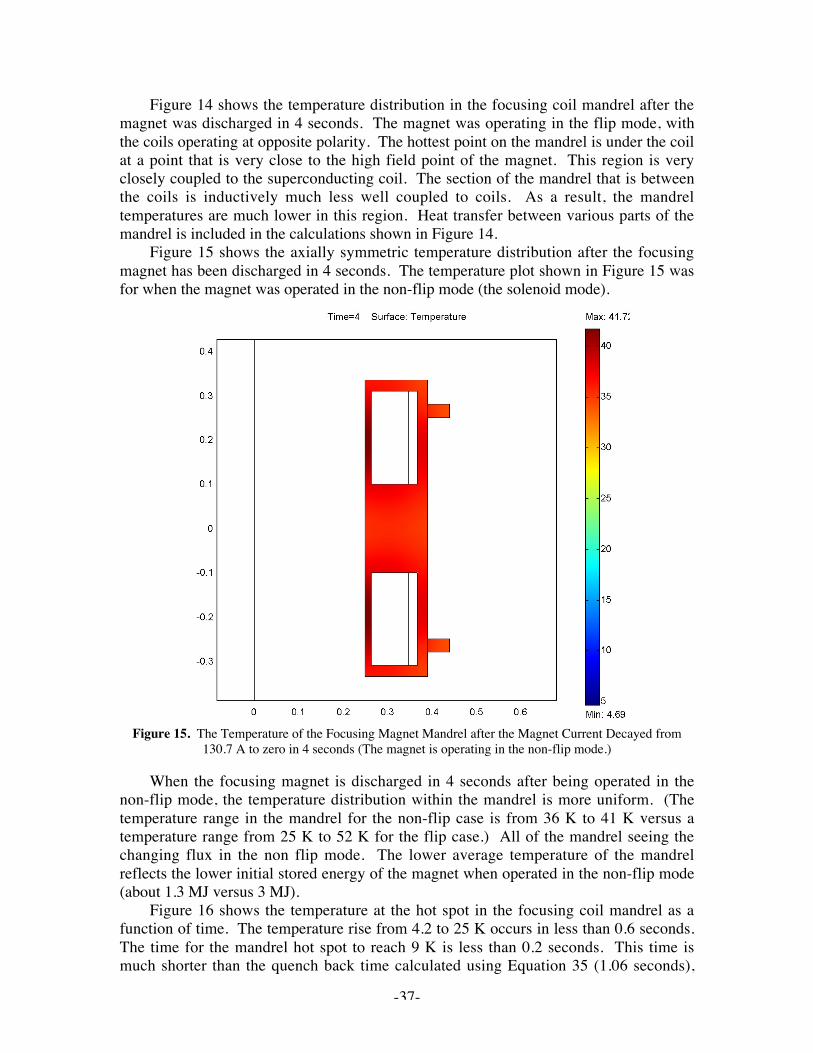
-37-

Figure 14 shows the temperature distribution in the focusing coil mandrel after themagnet was discharged in 4 seconds. The magnet was operating in the flip mode, withthe coils operating at opposite polarity. The hottest point on the mandrel is under the coilat a point that is very close to the high field point of the magnet. This region is veryclosely coupled to the superconducting coil. The section of the mandrel that is betweenthe coils is inductively much less well coupled to coils. As a result, the mandreltemperatures are much lower in this region. Heat transfer between various parts of themandrel is included in the calculations shown in Figure 14.

Figure 15 shows the axially symmetric temperature distribution after the focusingmagnet has been discharged in 4 seconds. The temperature plot shown in Figure 15 wasfor when the magnet was operated in the non-flip mode (the solenoid mode).

Figure 15. The Temperature of the Focusing Magnet Mandrel after the Magnet Current Decayed from130.7 A to zero in 4 seconds (The magnet is operating in the non-flip mode.)

When the focusing magnet is discharged in 4 seconds after being operated in thenon-flip mode, the temperature distribution within the mandrel is more uniform. (Thetemperature range in the mandrel for the non-flip case is from 36 K to 41 K versus atemperature range from 25 K to 52 K for the flip case.) All of the mandrel seeing thechanging flux in the non flip mode. The lower average temperature of the mandrelreflects the lower initial stored energy of the magnet when operated in the non-flip mode(about 1.3 MJ versus 3 MJ).

Figure 16 shows the temperature at the hot spot in the focusing coil mandrel as afunction of time. The temperature rise from 4.2 to 25 K occurs in less than 0.6 seconds.The time for the mandrel hot spot to reach 9 K is less than 0.2 seconds. This time ismuch shorter than the quench back time calculated using Equation 35 (1.06 seconds),

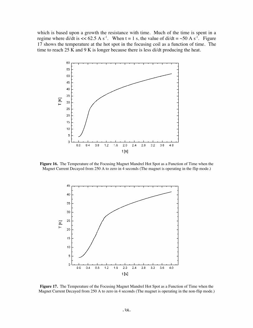
-38-

which is based upon a growth the resistance with time. Much of the time is spent in aregime where di/dt is << 62.5 A s-1. When t = 1 s, the value of di/dt = ~50 A s-1. Figure17 shows the temperature at the hot spot in the focusing coil as a function of time. Thetime to reach 25 K and 9 K is longer because there is less di/dt producing the heat.

Figure 16. The Temperature of the Focusing Magnet Mandrel Hot Spot as a Function of Time when theMagnet Current Decayed from 250 A to zero in 4 seconds (The magnet is operating in the flip mode.)

Figure 17. The Temperature of the Focusing Magnet Mandrel Hot Spot as a Function of Time when theMagnet Current Decayed from 250 A to zero in 4 seconds (The magnet is operating in the non-flip mode.)

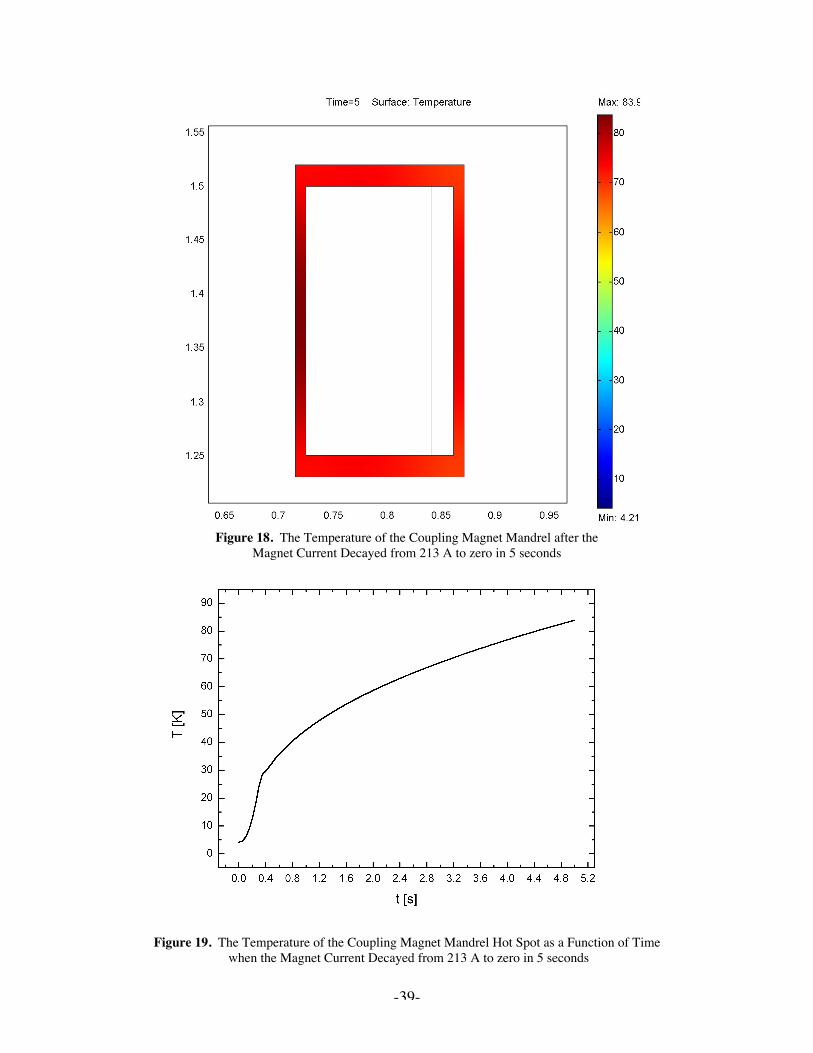
-39-

Figure 18. The Temperature of the Coupling Magnet Mandrel after theMagnet Current Decayed from 213 A to zero in 5 seconds

Figure 19. The Temperature of the Coupling Magnet Mandrel Hot Spot as a Function of Time when the Magnet Current Decayed from 213 A to zero in 5 seconds

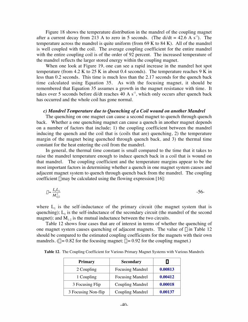
-40-

Figure 18 shows the temperature distribution in the mandrel of the coupling magnetafter a current decay from 213 A to zero in 5 seconds. (The di/dt = 42.6 A s-1). Thetemperature across the mandrel is quite uniform (from 69 K to 84 K). All of the mandrelis well coupled with the coil. The average coupling coefficient for the entire mandrelwith the entire coupling coil is of the order of 92 percent. The increased temperature ofthe mandrel reflects the larger stored energy within the coupling magnet.

When one look at Figure 19, one can see a rapid increase in the mandrel hot spottemperature (from 4.2 K to 25 K in about 0.4 seconds). The temperature reaches 9 K inless than 0.2 seconds. This time is much less than the 2.17 seconds for the quench backtime calculated using Equation 35. As with the focusing magnet, it should beremembered that Equation 35 assumes a growth in the magnet resistance with time. Ittakes over 5 seconds before di/dt reaches 40 A s-1, which only occurs after quench backhas occurred and the whole coil has gone normal.

c) Mandrel Temperature due to Quenching of a Coil wound on another MandrelThe quenching on one magnet can cause a second magnet to quench through quench

back. Whether a one quenching magnet can cause a quench in another magnet dependson a number of factors that include; 1) the coupling coefficient between the mandrelinducing the quench and the coil that is (coils that are) quenching, 2) the temperaturemargin of the magnet being quenched through quench back, and 3) the thermal timeconstant for the heat entering the coil from the mandrel.

In general, the thermal time constant is small compared to the time that it takes toraise the mandrel temperature enough to induce quench back in a coil that is wound onthat mandrel. The coupling coefficient and the temperature margins appear to be themost important factors in determining whether a quench in one magnet system causes andadjacent magnet system to quench through quench back from the mandrel. The couplingcoefficient e may be calculated using the flowing expression [16]:

†

e =L1L2

M1-22 -56-

where L1 is the self-inductance of the primary circuit (the magnet system that isquenching); L2 is the self-inductance of the secondary circuit (the mandrel of the secondmagnet); and M1-2 is the mutual inductance between the two circuits.

Table 12 shows four cases that are of interest in terms of whether the quenching ofone magnet system causes quenching of adjacent magnets. The value of e in Table 12should be compared to the estimated coupling coefficients for the magnets with their ownmandrels. (e = 0.82 for the focusing magnet; e = 0.92 for the coupling magnet.)

Table 12. The Coupling Coefficient for Various Primary Magnet Systems with Various Mandrels

Primary Secondary e

2 Coupling Focusing Mandrel 0.008131 Coupling Focusing Mandrel 0.00412

3 Focusing Flip Coupling Mandrel 0.000183 Focusing Non-flip Coupling Mandrel 0.00137

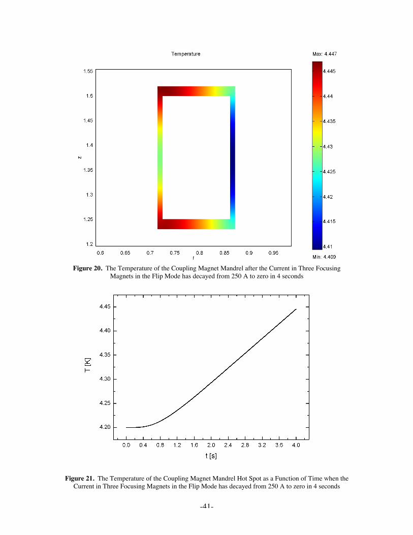
-41-

Figure 20. The Temperature of the Coupling Magnet Mandrel after the Current in Three FocusingMagnets in the Flip Mode has decayed from 250 A to zero in 4 seconds

Figure 21. The Temperature of the Coupling Magnet Mandrel Hot Spot as a Function of Time when theCurrent in Three Focusing Magnets in the Flip Mode has decayed from 250 A to zero in 4 seconds

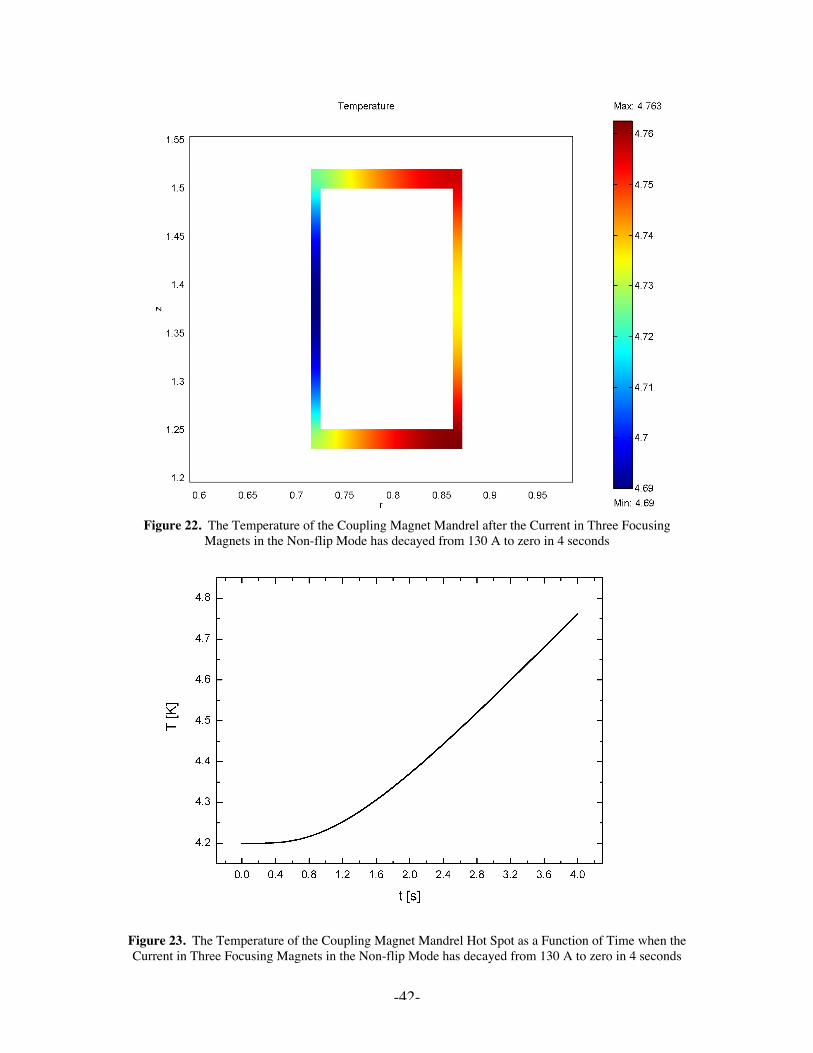
-42-

Figure 22. The Temperature of the Coupling Magnet Mandrel after the Current in Three FocusingMagnets in the Non-flip Mode has decayed from 130 A to zero in 4 seconds

Figure 23. The Temperature of the Coupling Magnet Mandrel Hot Spot as a Function of Time when theCurrent in Three Focusing Magnets in the Non-flip Mode has decayed from 130 A to zero in 4 seconds

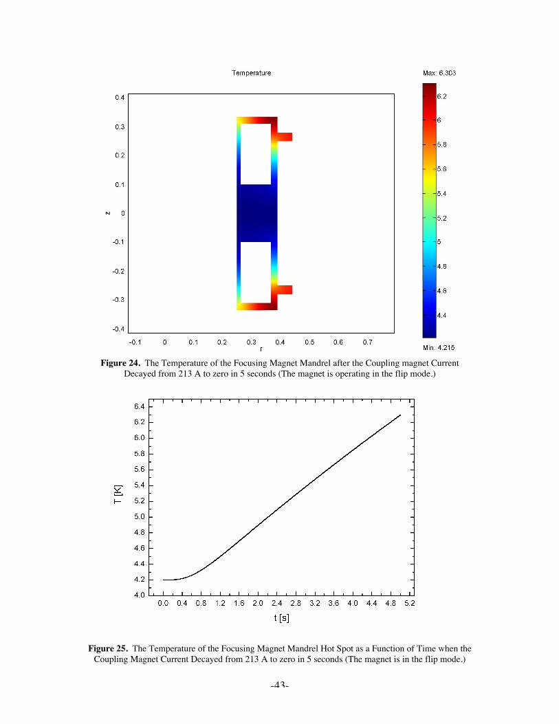
-43-

Figure 24. The Temperature of the Focusing Magnet Mandrel after the Coupling magnet CurrentDecayed from 213 A to zero in 5 seconds (The magnet is operating in the flip mode.)

Figure 25. The Temperature of the Focusing Magnet Mandrel Hot Spot as a Function of Time when theCoupling Magnet Current Decayed from 213 A to zero in 5 seconds (The magnet is in the flip mode.)

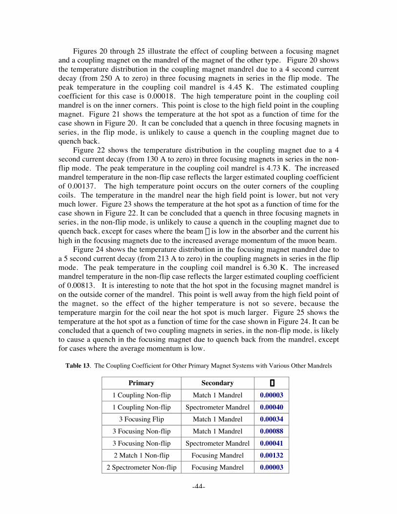
-44-

Figures 20 through 25 illustrate the effect of coupling between a focusing magnetand a coupling magnet on the mandrel of the magnet of the other type. Figure 20 showsthe temperature distribution in the coupling magnet mandrel due to a 4 second currentdecay (from 250 A to zero) in three focusing magnets in series in the flip mode. Thepeak temperature in the coupling coil mandrel is 4.45 K. The estimated couplingcoefficient for this case is 0.00018. The high temperature point in the coupling coilmandrel is on the inner corners. This point is close to the high field point in the couplingmagnet. Figure 21 shows the temperature at the hot spot as a function of time for thecase shown in Figure 20. It can be concluded that a quench in three focusing magnets inseries, in the flip mode, is unlikely to cause a quench in the coupling magnet due toquench back.

Figure 22 shows the temperature distribution in the coupling magnet due to a 4second current decay (from 130 A to zero) in three focusing magnets in series in the non-flip mode. The peak temperature in the coupling coil mandrel is 4.73 K. The increasedmandrel temperature in the non-flip case reflects the larger estimated coupling coefficientof 0.00137. The high temperature point occurs on the outer corners of the couplingcoils. The temperature in the mandrel near the high field point is lower, but not verymuch lower. Figure 23 shows the temperature at the hot spot as a function of time for thecase shown in Figure 22. It can be concluded that a quench in three focusing magnets inseries, in the non-flip mode, is unlikely to cause a quench in the coupling magnet due toquench back, except for cases where the beam b is low in the absorber and the current hishigh in the focusing magnets due to the increased average momentum of the muon beam.

Figure 24 shows the temperature distribution in the focusing magnet mandrel due toa 5 second current decay (from 213 A to zero) in the coupling magnets in series in the flipmode. The peak temperature in the coupling coil mandrel is 6.30 K. The increasedmandrel temperature in the non-flip case reflects the larger estimated coupling coefficientof 0.00813. It is interesting to note that the hot spot in the focusing magnet mandrel ison the outside corner of the mandrel. This point is well away from the high field point ofthe magnet, so the effect of the higher temperature is not so severe, because thetemperature margin for the coil near the hot spot is much larger. Figure 25 shows thetemperature at the hot spot as a function of time for the case shown in Figure 24. It can beconcluded that a quench of two coupling magnets in series, in the non-flip mode, is likelyto cause a quench in the focusing magnet due to quench back from the mandrel, exceptfor cases where the average momentum is low.

Table 13. The Coupling Coefficient for Other Primary Magnet Systems with Various Other Mandrels

Primary Secondary e

1 Coupling Non-flip Match 1 Mandrel 0.000031 Coupling Non-flip Spectrometer Mandrel 0.00040

3 Focusing Flip Match 1 Mandrel 0.000343 Focusing Non-flip Match 1 Mandrel 0.000883 Focusing Non-flip Spectrometer Mandrel 0.000412 Match 1 Non-flip Focusing Mandrel 0.00132

2 Spectrometer Non-flip Focusing Mandrel 0.00003

-45-

From Table 13 it is clear that coupling between the cooling channel magnets (thefocusing and coupling magnets) and the detector magnets is small. Since thetemperature margin for all of the detector magnets is large (about 2 K), it is unlikely thatany of the detector magnet circuits will be driven normal through quench back from themandrel. From Table 13 it is also clear that quenching the spectrometer magnet isunlikely to quench the focusing magnets directly. At high momenta, when thetemperature margin in the focus magnets is small, a quench of the first match coil maycause a quench in the focusing magnet system.

Concluding Comments

This report shows that the MICE magnets can be quenched safely. The MICEchannel coils are short and relatively thin. Thus a whole focus coil or coupling coil willturn completely normal relatively quickly once the coil starts to quench. A relatively lowresistance in the magnet circuit is needed to cause either the focusing magnet or thecoupling magnet to turn normal through quench back from the magnet mandrel.Reducing the magnet mandrel resistivity reduces the magnet quench back time.Unfortunately, one cannot reduce the quench back time by reducing the mandrelresistivity. High electrical resistivity is inherent to 6061-T6 aluminum. Aluminum witha lower electrical resistivity will not be strong enough to carry the magnetic forces.

No active external quench protection system is needed for any of the MICE magnets.The three focusing magnets can be quenched passively while hooked together in eitherthe flip mode or non-flip mode. The coupling magnets can also be connected in series,but the hot spot temperature in the quenched coil will go up. It is recommended that thecoupling coils be powered separately, in order to reduce the charge time so that thecoupling magnets can be charged in the same time as the other magnets.

The focusing magnets will have warm diodes and resistors across their coils. Thediodes and resistors will reduce the voltage buildup in the magnet circuit as the magnetstring is quenching. The coupling magnet will be sub-divided into magnet sub-circuits.Each sub-circuit will have a cold diode and resistor across the sub-circuit to limit thevoltage build up during the quench process. The resistor across the inner sub-circuit ofthe coupling magnet can be used to speed up the magnet quench back process for thewhole magnet. This will further reduce voltage built up and the hot spot temperature inthe magnet that first quenches.

The MICE cooling channel magnets and the detector magnets form severalinductively coupled circuits. Charging or discharging one magnet circuit will induce avoltage in the other magnet circuits. The power supplies must be capable of regulatingthe current in all of the MICE magnet circuits while all magnets are being charged.

Six 300 A, 10 V power supplies are required for MICE. Six 50 A, 10 V powersupplies are required for correction of the two spectrometer end coils and for correctionof the current in the two end focus coils at the ends of the cooling channel. It isrecommended that a six-phase power supply (after half wave rectification) be used inorder to reduce the voltage ripple, but a two-phase power supply (after half waverectification) may provide a low enough voltage ripple to ensure that the current ripplewill be less than 0.03 percent. The power supply current regulation should also be goodto 0.03 percent.

-46-

Detailed simulations of coupling from the magnet coils to the mandrel show that theparts of the mandrel that are closest to the magnet coils are better coupled than the partsof the mandrel furthest from the coil current center. When the magnet is charged ordischarged at a uniform rate, the current flowing in the mandrel is proportional to di/dtand inversely proportional to the mandrel material resistivity. The energy put into themandrel inductively is inversely proportional to the charge or discharge time. It is clear,from the simulation, that quenching the magnet heats the mandrel.

It is also clear that quenching a magnet heats the mandrels of other magnets that arecoupled to the magnet quenching. The quenching of the focusing magnet is unlikely toquench any other magnet in MICE when the machine operates in the flip mode. In thenon-flip mode, a quench of the focusing magnets can cause quenching of other magnetswhen these magnets are operating at a temperature that is close to the critical temperatureof the superconductor at the high field point. Quenching the coupling coil will quenchthe focusing magnets when the temperature margin is less than about 1.5 K in the flipmode. Quenching the coupling magnets can also cause quenching of the focusingmagnets in the non-flip mode for the very low muon beam beta in the AFC module cases.A quench of the detector solenoid may cause the focusing coils to quench when thefocusing magnet temperature margin is low. Quenching the focusing or the couplingmagnets is unlikely to quench any of the detector magnets.

Acknowledgements

This work was supported by the Oxford University Physics Department and theParticle Physics and Astronomy Research Council of the United Kingdom. This workwas also supported by the Lawrence Berkeley Laboratory and the Office of Science,United States Department of Energy, under the DOE contract DE-AC03-76SF00098.

References

[1] "A Proposal to the Rutherford Appleton Laboratory, an International MuonIonization Cooling Experiment (MICE)," proposed by the MICE Collaboration,15 December 2002

[2] G. Gregoire, G. Ryckewaert, L. Chevalier, et al, “MICE and International MuonIonization Cooling Experiment Technical Reference Document,”(October 2004)

[3] W. H. Cherry and J. I Gittlemen, “Thermal and Electrodynamic Aspects of theSuperconductive Transition Process,” Solid State Electronics 1, p 287 (1960)

[4] A. V. Tollestrup Fermi National Laboratory, private communication about 1975[5] P. H. Eberhard, M. Alston-Gernjost, M. A. Green, et al, “Quenches in Large

Superconducting Magnets,” Proceedings of MT-6, Bratislava, Czechoslovakia,p 654, (1977) also LBL-6718 (August 1977)

[6] Z. J. J. Stekly, “Theoretical and Experimental Study of an UnprotectedSuperconducting Coil Going Normal,” Advances in Cryogenic Engineering 8,p. 585, Plenum Press, New York, (1962)

[7] M. Scherer and P. Turowski, "Investigation of the Propagation Velocity of aNormal Conducting Zone in Technical Superconductors," Cryogenics 18 p. 515(September 1978)

-47-

[8] P. H. Eberhard et al., "The Measurement and Theoretical Calculation of QuenchVelocities in Large Fully Epoxy Impregnated Superconducting Coils," IEEETransactions on Magnetics, MAG-17, No. 5, pp. 1803, (1981)

[9] M. A. Green, "The Role of Quench Back in Quench Protection of aSuperconducting Solenoid", Cryogenics 24, p 659, (December 1984).

[10] J. D. Taylor, et al, "Quench Protection for a 2 MJ Magnet", IEEE Transactionson Magnetics MAG-15, No. 1, p. 855, (1979)

[11] M. A. Green, "Design Conditions for Fail-Safe Quenching of a High-CurrentDensity Superconducting Solenoid Magnet with a Shorted Secondary Circuit",LBL-14859, September 1982.

[12] M. A. Green, "Quench Back in Thin Superconducting Solenoid Magnets",Cryogenics 24, p 3, (1984)

[13] Jon Zbasnik of the Lawrence Berkeley Laboratory, private communicationconcerning the failure of one of the ALS Superbend RDK-415D coolers.

[14] M. A. Green and S. Q. Yang, “Heat Transfer into and within the 4.4 K Regionand the 40 K Shields of the MICE Focusing and Coupling Magnets,” OxfordUniversity Physics Department Report for the MICE project, 28 April 2004

[15] Handbook of Materials for Superconducting Machinery, Metal and CeramicsInformation Center, MIC-MB-04, National Bureau of Standards, Jan. 1977

[16] W. R. Smythe, Static and Dynamic Electricity, McGraw Hill Book Co., NewYork, (1950)

[17] L. Li, “High Performance Pulsed Magnets: Theory, Design and Construction.PhD Thesis, Katholieke Universiteit Leuven, Belgium, 1998.

[18] A. Führer, K. Heidemann and W. Nerreter, Grundgebiete der Elektrotechnik,Band 2: Zeitabhängige Vorgänge, Carl Hanser Verlag, München, 1994.

[19] G. K. White and P. J. Meeson. Experimental Techniques in Low-TemperaturePhysics. Oxford University Press, Oxford, 2002.

[20] Femlab 3 Electromagnetic Module User’s Guide. COMSOL, 2004.[21] Femlab 3 Modelling Guide. COMSOL, 2004.[22] J. D. Jackson. Classical Electrodynamics. 3rd edition, John Weiley & Sons, 1998.