Embed Size (px)
Citation preview
7/22/2019 Quaternions for engineers
http://slidepdf.com/reader/full/quaternions-for-engineers 1/12
SUBMITTED TO THE IEEE TRANSACTIONS ON ROBOTICS 1
Approaching Dual Quaternions
From Matrix AlgebraFederico Thomas, Member, IEEE
Abstract—Dual quaternions give a neat and succinct wayto encapsulate both translations and rotations into a unifiedrepresentation that can easily be concatenated and interpolated.Unfortunately, the combination of quaternions and dual numbersseem quite abstract and somewhat arbitrary when approachedfor the first time. Actually, the use of quaternions or dual num-bers separately are already seen as a break in mainstream robotkinematics, which is based on homogeneous transformations. Thispaper shows how dual quaternions arise in a natural way whenapproximating 3D homogeneous transformations by 4D rotationmatrices. This results in a seamless presentation of rigid-bodytransformations based on matrices and dual quaternions whichpermits building intuition about the use of quaternions and theirgeneralizations.
Index Terms—Spatial kinematics, quaternions, biquaternions,double quaternions, dual quaternions, Cayley factorization.
I. INTRODUCTION
IN 1843, Hamilton defined quaternions as quadruples of the
form a + bi + cj + dk, where i2 = j2 = k2 = ij k = −1,
when seeking a new kind of number that would extend the
idea of complex numbers [1].
Quaternions were developed independently of their needs
for any particular application. The main use of quaternions
in the nineteenth century consisted in expressing physical
theories in the notation of quaternions. In this context, duringthe end of the nineteenth century, researchers working on
electromagnetic theory debated about the choice of quaternion
or vector notation in their formulations. This generated a fierce
dispute from about 1880 to 1900, reaching its climax in a
series of letters in the journal Nature [2]. Then, quaternions
disappeared from view, and their value discredited, having
been replaced by the simpler algebra of matrices and vectors.
Later on, in the mid-twentieth century, the development of
computing machinery made necessary a re-examination of
quaternions from the standpoint of their utility in computer
simulations. The need for efficient simulations of aircraft and
missile motions was responsible to a large extent for sparking
the renewed interest in quaternions [3]. It was rapidly realized
that quaternion algebra yields more efficient algorithms than
matrix algebra for applications involving rigid-body transfor-
mations. Nowadays, quaternions play a fundamental role in
the representation of spatial rotations and a chapter devoted
to them can be found in nearly every advanced textbook
F. Thomas is with the Instit ut de Robotica i Informatica In-dustrial (CSIC-UPC), Llorens Artigas 4-6, 08028 Barcelona, [email protected]
This work was supported by the Spanish Ministry of Economy andCompetitiveness through the Explora programme under Contract DPI2011-13208-E.
on Computer Vision, Robot Kinematics and Dynamics, or
Computer Graphics.
Surprisingly, despite their long life, the use of quaternions in
engineering is not free from confusions which mainly concern:
1) The order of quaternion multiplication. Quaternions are
sometimes multiplied in the opposite order than rotation
matrices, as in [4]. The origin of this can be found in
the way vector coordinates are represented. For example,
in [5], a celebrated book on Computer Graphics, point
coordinates are represented by row vectors instead of
column vectors, as is the common practice in Robotics.Then, transformation matrices post-multiply a point
vector to produce a new point vector. When using
quaternions, instead of homogeneous transformations,
the same composition rules are adopted. The result can
be confusing for anyone approaching quaternions for the
first time. For more details on this matter, see [6].
2) The way quaternions operate on vectors. Quaternions
have been used to rotate vectors in three dimensions
by essentially sandwiching a vector in three dimensions
between a unit quaternion and its conjugate [7, Chap. 17]
[8]. Nevertheless, strictly speaking, quaternions cannot
operate on vectors. The word vector was introduced by
Hamilton to denote the imaginary part of the quaternion
which is different from today’s meaning [9].
3) The nature of the quaternion imaginary units [6], [8].
Hamilton himself contributed to this confusion as he
always identified the quaternion units with quadrantal
rotations, as he called the rotations by π/2 [10, p. 64,
art. 71]. Nevertheless, they represent rotations by π [9].
All these confusions are seriously affecting the progress of
quaternions in engineering because, as a result, they are used
in recipes for manipulating sequences of rotations without
a precise understanding of their meaning. The situation just
worsens when working with dual quaternions, an extension of ordinary quaternions that permits encapsulating rotations and
translations in a unified representation. Thus, it is not strange
that many practitioners are still averse to using them despite
their undeniable value.
This paper shows how quaternions do naturally emerge
from 4D rotation matrices and how dual quaternions are then
derived when approximating 3D homogeneous transformations
by 4D rotations. As a consequence, all common misun-
derstandings concerning quaternions are cleared up because
the derived expressions may be interpreted both as matrix
expressions and as quaternions.
7/22/2019 Quaternions for engineers
http://slidepdf.com/reader/full/quaternions-for-engineers 2/12
SUBMITTED TO THE IEEE TRANSACTIONS ON ROBOTICS 2
A. Quaternions and rotations in R3 and R4
Soon after Hamilton introduced quaternions, he tried to
use them to represent rotations in R3 in the same way as
complex numbers can be used to represent rotations in R2.
Nevertheless, it seems that he was not aware of Rodrigues’
work and his use of quaternions as a description of rotations
was wrong. He believed that the expression for a rotated
vector was linear in the quaternion rather than quadratic. Thispassage of the history of quaternions is actually a matter of
controversy (see [9], [11], [12] for details). It is Cayley whom
we must thank for the correct development of quaternions as a
representation of rotations and for establishing the connection
with the results published by Rodrigues three years before the
discovery of quaternions [13]. Cayley is also credited to be
the first to discover that quaternions could also be used to
represent rotations in R4 [14]. Cayley’s results can be used
to prove that any rotation in R4 is a product of rotations
in a pair of orthogonal two-dimensional subspaces [15]. This
factorization, known as Cayley’s factoring of 4D rotations,
was also proved using matrix algebra by Van Elfrinkhof in
1897 in a paper [16] rescued from oblivion by Mebius in [17].Cayley’s factorization plays a central role in what follows as it
provides a bridge between homogeneous transformations and
quaternions that remained unnoticed in the past.
B. Quaternions and their generalizations
In 1882, Clifford introduced the idea of a biquaternion in
three papers: “Preliminary sketch of biquaternions”, “ Notes
on biquaternions”, and “Further note on biquaternions” [18]
(see [19] for a review and summary of this work). Clifford
adopted the word biquaternion, previously used by Hamilton
to refer to a quaternion with complex coefficients, to denote a
combination of two quaternions algebraically combined via anew symbol, ω, defined to have the property ω2 = 0, so that
a biquaternion has the form q 1 + ωq 2, where q 1 and q 2 are
both ordinary quaternions. The use of the term biquaternion
is confusing. As observed in [19], even Clifford contributed
to this confusion by using the symbol ω in several different
contexts. For example, in his paper “Preliminary sketch of
biquaternions paper ”, it is also used with the multiplication
rule ω2 = 1. Nowadays, in the area of robot kinematics,
biquaternions of the form q 1 + εq 2, where ε2 = 0, are called
dual quaternions, while those of the form q 1 + eq 2, where
e2 = 1, are called double quaternions. This denomination
derives from the fact that the symbols ε and e designate the
dual and the double units, respectively [20]. Thus, we havethree imaginary units which can be equal either to the complex
unit i (i2 = −1), to the dual unit ε (ε2 = 0), or to the double
unit e (e2 = 1). These units define the basis of the so-called
hypercomplex numbers [21].
The double quaternion q 1 + eq 2 can be reformulated by
introducing the symbols ξ = 1+e2
and η = 1−e2
[18], [22].
Then, q 1 + eq 2 = ξ (q 1 + q 2) + η(q 1 − q 2). Since ξ 2 = ξ ,η2 = η and ξη = 0, the terms (q 1 + q 2) and (q 1 − q 2)operate independently in the double quaternion product which
has been found quite convenient when manipulating kinematic
equations expressed in terms of double quaternions [23]. A
third possible representation for double quaternions consists
in having two quaternions expressed in different bases of
imaginary units whose product is commutative. This also leads
to couples of quaternions that operate independently when
multiplied. Nowadays, the algebras of ordinary, double, and
dual quaternions are grouped under the umbrella of Clifford
algebras, also known as geometric algebras (see [24, Chap. 9]
or [25] for an introduction).
While double quaternions have been found direct applica-
tion to represent 4D rotations, dual quaternions found ap-
plication to encapsulate both translation and rotation into a
unified representation. Then, if 3D spatial displacements are
approximated by 4D rotations, a beautiful connection between
double and dual quaternions can be established.
Yang and Freudenstein introduced the use of dual quater-
nions for the analysis of spatial mechanisms [26]. Since
then, dual quaternions have been used by several authors in
the kinematic analysis and synthesis of mechanisms, and in
computer graphics (see, for instance, the works of McCarthy
[27], Angeles [28], and Perez-Gracia [29]).
C. Quaternions and matrix algebra
Matrix algebra was developed beginning about 1858 by
Cayley and Sylvester. Soon it was realized that matrices
could be used to represent the imaginary units used in the
definition of quaternions. Actually, a set of 4 × 4 matrices,
sometimes called Dirac-Eddington-Conway matrices, with real
values can realize every algebraic requirement of quaternions.
Alternatively, a set of 2 × 2 matrices, usually called Pauli
matrices, with complex values can play the same role (see [30,
pp. 143-144] for details). Therefore, there are sets of matrices
which all produce valid matrix representations of quaternions.
The choice of one set over other has been driven by esthetic
preferences, but we will show how Cayley’s factorization
leads to a matrix representation that attenuates this sense of
arbitrariness.
While in most textbooks the matrix representation of quater-
nions is considered as an advanced topic, if ever mentioned,
in this paper matrix algebra is used as the doorway to quater-
nions. This would probably be the usual practice if matrix
algebra had been developed before quaternions.
D. Organization of the paper
This paper is organized as follows. Section II reviews the
connection between 4D rotations and double quaternions in
terms of matrix algebra. Section III presents a digression, thatcan be skipped on a first reading, in which the expressive
power of matrix algebra is explored to derive different systems
of hypercomplex numbers associated with 4D rotations. In
Section IV, the results presented in Section II are specialized
to the 3D case. Section V deals with the problem of ap-
proximating 3D transformations in homogeneous coordinates
by 4D rotations. The results obtained in Section IV and
Section V constitute the basic building blocks of the proposed
twofold matrix-quaternion formalism for the representation
of rigid-body transformations. The reinterpretation of kine-
matic equations expressed as products of transformations in
7/22/2019 Quaternions for engineers
http://slidepdf.com/reader/full/quaternions-for-engineers 3/12
SUBMITTED TO THE IEEE TRANSACTIONS ON ROBOTICS 3
homogeneous coordinates using this formalism is treated in
Section VI. Section VII presents some examples and, finally,
we conclude in Section VIII with a summary of the main
points.
II. 4D ROTATIONS AND DOUBLE QUATERNIONS
After a proper change in the orientation of the reference
frame, an arbitrary 4D rotation matrix (i.e., an orthogonalmatrix with determinant +1) can be expressed as [31, Theorem
4]: cos α1 − sin α1 0 0sin α1 cos α1 0 0
0 0 cos α2 − sin α2
0 0 sin α2 cos α2
. (1)
Thus, a 4D rotation is defined by two mutually orthogonal
planes of rotation, each of which is fixed in the sense that
points in each plane stay within the planes. Then, a 4D rotation
has two angles of rotation, α1 and α2, one for each plane of
rotation, through which points in the planes rotate. All points
not in the planes rotate through an angle between α1 and α2.
See [32] for details on the geometric interpretation of rotations
in four dimensions.
If α1 = ±α2, the rotation is called an isoclinic rotation. An
isoclinic rotation can be left- or right-isoclinic (depending on
whether α1 = α2 or α1 = −α2, respectively) which can be
represented by a rotation matrix of the form
RL =
l0 −l3 l2 −l1l3 l0 −l1 −l2
−l2 l1 l0 −l3l1 l2 l3 l0
, (2)
and
RR = r0 −r3 r2 r1r3 r0 −r1 r2−r2 r1 r0 r3−r1 −r2 −r3 r0
, (3)
respectively. Since (2) and (3) are rotation matrices, their rows
and columns are unit vectors. As a consequence,
l21 + l22 + l23 + l24 = 1 (4)
and
r21 + r22 + r23 + r24 = 1. (5)
Without loss of generality, we have introduced some
changes in the signs and indices of (2) and (3) with respect to
the notation used by Cayley [14], [33] to ease the treatmentgiven below and to provide a neat connection with the stan-
dard use of quaternions for representating rotations in three
dimensions.
Isoclinic rotation matrices have three important properties:
1) The product of two right- (left-) isoclinic matrices is a
right- (left-) isoclinic matrix.
2) The product of a right- and a left-isoclinic matrix is
commutative.
3) Any 4D rotation matrix, according to Cayley’s factor-
ization, can be decomposed into the product of a right-
and a left-isoclinic matrix.
Then, a 4D rotation matrix, say R, can be expressed as:
R = RLRR = RRRL (6)
where
RL = l0I + l1A1 + l2A2 + l3A3 (7)
and
RR = r0I + r1B1 + r2B2 + r3B3, (8)
where I stands for the 4 × 4 identity matrix and
A1 =
0 0 0 −10 0 −1 00 1 0 01 0 0 0
, A2 =
0 0 1 00 0 0 −1
−1 0 0 00 1 0 0
,
A3 =
0 −1 0 01 0 0 00 0 0 −10 0 1 0
, B1 =
0 0 0 10 0 −1 00 1 0 0
−1 0 0 0
,
B2 =
0 0 1 00 0 0 1
−1 0 0 0
0 −1 0 0
, B3 =
0 −1 0 01 0 0 00 0 0 1
0 0 −1 0
.
Therefore, {I, A1, A2, A3} and {I, B1, B2, B3} can be seen,
respectively, as bases for left- and right-isoclinic rotations.
The details on how to compute Cayley’s factorization (6)
can be found in the appendix.
Now, it can be verified that
A21 = A2
2 = A23 = A1A2A3 = −I, (9)
and
B21 = B2
2 = B23 = B1B2B3 = −I. (10)
We can recognize in these two expressions the quaternion
definition. Actually, (9) and (10) reproduce the celebrated
formula that Hamilton carved into the stone of Brougham
Bridge.
Expression (9) determines all the possible products of A1,
A2, and A3 resulting in
A1A2 = A3, A2A3 = A1, A3A1 = A2,
A2A1 = −A3, A3A2 = −A1, A1A3 = −A2. (11)
Likewise, all the possible products of B1, B2, and B3 can
be derived from expression (10). All these products can be
summarized in the following product tables:
I A1 A2 A3
I I A1 A2 A3
A1 A1 −I A3 −A2
A2 A2 −A3 −I A1
A3 A3 A2 −A1 −I
(12)
I B1 B2 B3
I I B1 B2 B3
B1 B1 −I B3 −B2
B2 B2 −B3 −I B1
B3 B3 B2 −B1 −I
(13)
Moreover, it can be verified that
AiBj = BjAi. (14)
7/22/2019 Quaternions for engineers
http://slidepdf.com/reader/full/quaternions-for-engineers 4/12
SUBMITTED TO THE IEEE TRANSACTIONS ON ROBOTICS 4
which is actually a consequence of the commutativity of left-
and right-isoclinic rotations. Then, in the composition of two
4D rotations, we have:
R1R2 = (RL1 RR
1 )(RL2 RR
2 ) = (RL1 RL
2 )(RR1 RR
2 ). (15)
It can be concluded that RLi and RR
i can be seen either as
4×
4 rotation matrices or, when expressed as in (7) and (8)
respectively, as unit quaternions and their product, as a double
quaternion because they operate independently in the product
of two 4D rotations. It is said that they are unit quaternions
because their coefficients satisfy (4) and (5).
Next, in Section IV, the above twofold matrix-quaternion
representation of 4D rotations is specialized to 3D rotations
and, in Section V, generalized to represent 3D translations.
Nevertheless, let us fist explore this twofold representation a
bit further.
III. A DIGRESSION
One of the multiple advantages of the proposed matrix-
quaternion formulation is that the involved imaginary unitshave a clear algebraic interpretation. We can operate with these
units to obtain different representations of 4D rotations that
would otherwise be quite abstract and difficult to derive. To
see this, let us start by defining
D1 = A1B−11 =
−1 0 0 00 1 0 00 0 1 00 0 0 −1
,
D2 = −A2B−12 =
1 0 0 00 −1 0 00 0 1 00 0 0 −1
,
D3 = A3B−13 =
−1 0 0 00 −1 0 00 0 1 00 0 0 1
.
Then, it can be verified that
D21 = D2
2 = D23 = D1D2D3 = I (16)
which allow us to define a kind of quaternion whose imaginary
units are double units. As with ordinary quaternions, (16)
determines all the possible products of D1, D2, and D3 which
can be summarized in the following product table:
I D1 D2 D3
I I D1 D2 D3
D1 D1 I D3 D2
D2 D2 D3 I D1
D3 D3 D2 D1 I
(17)
Then, clearly Di = D−1i , i = 1, 2, 3, and, as a consequence,
B1 = D1A1, B2 = −D2A2, and B3 = D3A3.
Substituting the above expressions for Bi, i = 1, 2, 3, in (8),
multiplying the result by (7), and factoring out Di, i = 1, 2, 3,
we conclude that (6) can be rewritten as:
R = IQ0 + D1Q1 + D2Q2 + D3Q3 (18)
where
Q0 = r0 (l0I + l1A1 + l2A2 + l3A3) ,
Q1 = r1 (l0A1 − l1I + l2A3 − l3A2) ,
Q2 = r2 (−l0A2 + l1A3 + l2I − l3A1) ,
Q3 = r3 (l0A3 + l1A2 − l2A1 − l3I) .
Now, we can shift from the basis {I, D1, D2, D3} to thebasis {E1, E2, E3, E4} defined as
E1 = 1
4 (I − D1 + D2 − D3) =
1 0 0 00 0 0 00 0 0 00 0 0 0
, (19)
E2 = 1
4 (I + D1 − D2 − D3) =
0 0 0 00 1 0 00 0 0 00 0 0 0
, (20)
E3 =
1
4 (I + D1 + D2 + D3) = 0 0 0 00 0 0 0
0 0 1 00 0 0 0
, (21)
E4 = 1
4 (I − D1 − D2 + D3) =
0 0 0 00 0 0 00 0 0 00 0 0 1
. (22)
The elements of this basis are distinguished by the fact that
their multiplication table is the simplest possible for a basis:
E1 E2 E3 E4
E1 E1 0 0 0
E2 0 E2 0 0
E3 0 0 E3 0E4 0 0 0 E4
By inverting the system of equations defined by (19)-(22),
we obtain:
I = E1 + E2 + E3 + E4
D1 = −E1 + E2 + E3 − E4
D2 = E1 − E2 + E3 − E4
D3 = −E1 − E2 + E3 + E4
Substituting these expressions in (18) and factoring out Ei,
for i = 1, . . . , 4, we obtain:
R = E1K1 + E2K2 + E3K3 + E4K4, (23)
where
K1 =Q0 − Q1 + Q2 − Q3
=(r0l0 + r1l1 + r2l2 + r3l3)I
+ (r0l1 − r1l0 − r2l3 + r3l2)A1
+ (r0l2 + r1l3 − r2l0 − r3l1)A2
+ (r0l3 − r1l2 + r2l1 − r3l0)A3,
7/22/2019 Quaternions for engineers
http://slidepdf.com/reader/full/quaternions-for-engineers 5/12
SUBMITTED TO THE IEEE TRANSACTIONS ON ROBOTICS 5
K2 =Q0 + Q1 − Q2 − Q3
=(r0l0 − r1l1 − r2l2 + r3l3)I
+ (r0l1 + r1l0 + r2l3 + r3l2)A1
+ (r0l2 − r1l3 + r2l0 − r3l1)A2
+ (r0l3 + r1l2 − r2l1 − r3l0)A3,
K3 =Q0 + Q1 + Q2 + Q3
=(r0l0 − r1l1 + r2l2 − r3l3)I
+ (r0l1 + r1l0 − r2l3 − r3l2)A1
+ (r0l2 − r1l3 − r2l0 + r3l1)A2
+ (r0l3 + r1l2 + r2l1 + r3l0)A3,
and
K4 =Q0 − Q1 − Q2 + Q3
=(r0l0 + r1l1 − r2l2 − r3l3)I
+ (r0l1 − r1l0 + r2l3 − r3l2)A1
+ (r0l2 + r1l3 + r2l0 + r3l1)A2
+ (r0l3−
r1l2−
r2l1 + r3l0)A3.
It is thus concluded that a 4D rotation can be expressed
as a linear combination of four quaternions. In the product of
two 4D rotations, these four quaternions operate independently
because E2i = Ei, for i = 1, 2, 3, 4, and EiEj = 0 if i =
j. The reader interested in further exploring the connections
between 4D rotations and different sets of imaginary units is
referred to [33] and [34].
IV. 3D ROTATIONS AND ORDINARY QUATERNIONS
We have seen how double quaternions naturally emerge
from Cayley’s factorization of 4D rotations into isoclinic
rotations. Now, we specialize this result to 3D rotations.The homogenous matrix transformation representing a ro-
tation by φ about the x axis is:
Rx(φ) =
1 0 0 00 cos(φ) − sin(φ) 00 sin(φ) cos(φ) 00 0 0 1
, (24)
which can be readily interpreted as a rotation in R4. Then, its
Cayley’s factorization into a right- and a left-isoclinic rotation,
using the procedure given in the appendix, yields
RLx
(φ) = 1
√ t2 + 1 1 0 0 −t0 1 −t 0
0 t 1 0t 0 0 1 (25)
and
RRx
(φ) = 1√
t2 + 1
1 0 0 t0 1 −t 00 t 1 0−t 0 0 1
, (26)
respectively, where we have introduced the change of variable
t = tanφ2
to obtain more amenable expressions. Then,
Rx(φ) =
1√ t2 + 1
(I + tA1)
1√ t2 + 1
(I + tB1)
.
(27)
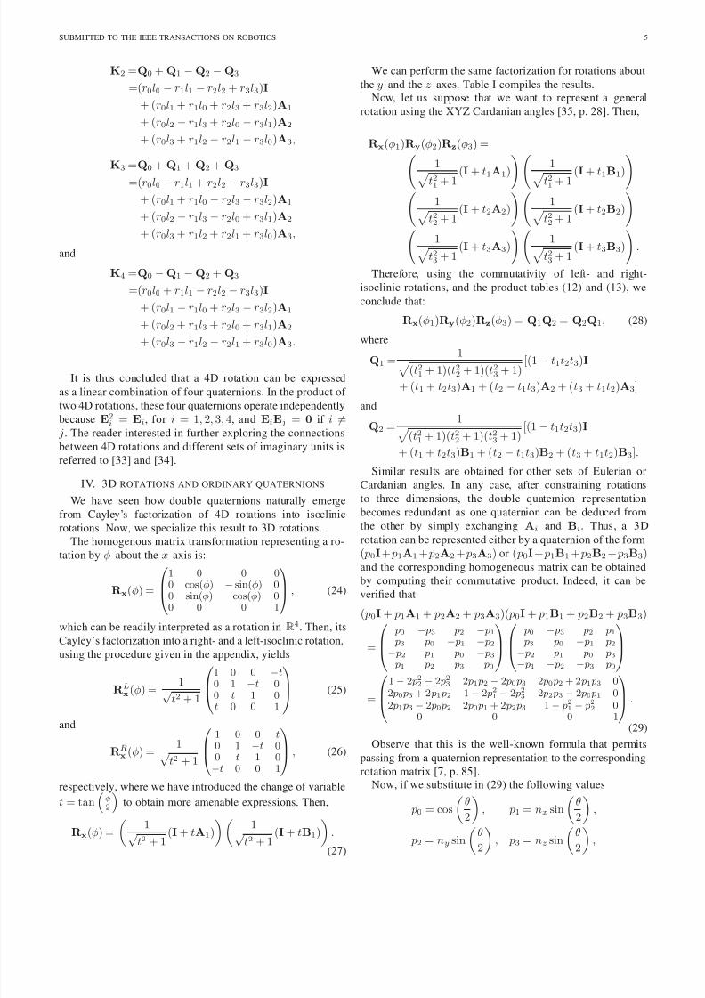
We can perform the same factorization for rotations about
the y and the z axes. Table I compiles the results.
Now, let us suppose that we want to represent a general
rotation using the XYZ Cardanian angles [35, p. 28]. Then,
Rx(φ1)Ry(φ2)Rz(φ3) =
1 t21 + 1 (I + t1A1) 1 t21 + 1 (I + t1B1) 1 t22 + 1
(I + t2A2)
1
t22 + 1(I + t2B2)
1 t23 + 1
(I + t3A3)
1
t23 + 1(I + t3B3)
.
Therefore, using the commutativity of left- and right-
isoclinic rotations, and the product tables (12) and (13), we
conclude that:
Rx(φ1)Ry(φ2)Rz(φ3) = Q1Q2 = Q2Q1, (28)
where
Q1 = 1
(t21 + 1)(t22 + 1)(t23 + 1)[(1 − t1t2t3)I
+ (t1 + t2t3)A1 + (t2 − t1t3)A2 + (t3 + t1t2)A3]
and
Q2 = 1
(t21 + 1)(t22 + 1)(t23 + 1)[(1 − t1t2t3)I
+ (t1 + t2t3)B1 + (t2 − t1t3)B2 + (t3 + t1t2)B3].
Similar results are obtained for other sets of Eulerian or
Cardanian angles. In any case, after constraining rotations
to three dimensions, the double quaternion representation
becomes redundant as one quaternion can be deduced from
the other by simply exchanging Ai and Bi. Thus, a 3Drotation can be represented either by a quaternion of the form
( p0I + p1A1 + p2A2 + p3A3) or ( p0I + p1B1 + p2B2 + p3B3)and the corresponding homogeneous matrix can be obtained
by computing their commutative product. Indeed, it can be
verified that
( p0I + p1A1 + p2A2 + p3A3)( p0I + p1B1 + p2B2 + p3B3)
=
p0 − p3 p2 − p1 p3 p0 − p1 − p2− p2 p1 p0 − p3 p1 p2 p3 p0
p0 − p3 p2 p1
p3 p0 − p1 p2− p2 p1 p0 p3− p1 − p2 − p3 p0
=1 − 2 p22 − 2 p23 2 p1 p2 − 2 p0 p3 2 p0 p2 + 2 p1 p3 02 p0 p3 + 2 p1 p2 1 − 2 p21 − 2 p23 2 p2 p3 − 2 p0 p1 02 p1 p3 − 2 p0 p2 2 p0 p1 + 2 p2 p3 1 − p21 − p22 0
0 0 0 1 .
(29)
Observe that this is the well-known formula that permits
passing from a quaternion representation to the corresponding
rotation matrix [7, p. 85].
Now, if we substitute in (29) the following values
p0 = cos
θ
2
, p1 = nx sin
θ
2
,
p2 = ny sin
θ
2
, p3 = nz sin
θ
2
,
7/22/2019 Quaternions for engineers
http://slidepdf.com/reader/full/quaternions-for-engineers 6/12
SUBMITTED TO THE IEEE TRANSACTIONS ON ROBOTICS 6
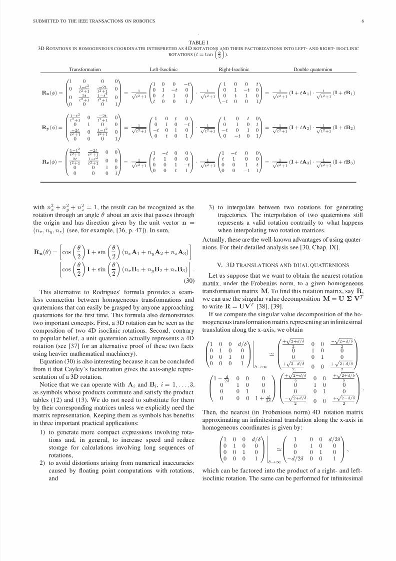
.
TABLE I3D ROTATIONS IN HOMOGENEOUS COORDINATES INTERPRETED AS 4 D ROTATIONS AND THEIR FACTORIZATIONS INTO LEFT- AND RIGHT- ISOCLINIC
ROTATIONS (t = tanφ2
).
Transformation Left-Isoclinic Right-Isoclinic Double quaternion
Rx(φ) =
1 0 0 0
0 1−t2
t2+1
−2tt2+1
0
0 2tt2+1
1−t2
t2+1 00 0 0 1
= 1
√ t2
+1
1 0 0 −t0 1 −t 0
0 t 1 0t 0 0 1
· 1
√ t2
+1
1 0 0 t0 1 −t 0
0 t 1 0−t 0 0 1
= 1
√ t2
+1
(I+ tA1)·
1
√ t2
+1
(I+ tB1)
Ry(φ) =
1−t2
t2+1 0 −2t
t2+1 0
0 1 0 0−2tt2+1
0 1−t2
t2+1 0
0 0 0 1
= 1√
t2+1
1 0 t 00 1 0 −t−t 0 1 00 t 0 1
· 1√
t2+1
1 0 t 00 1 0 t−t 0 1 00 −t 0 1
= 1√
t2+1(I+ tA2) · 1√
t2+1(I+ tB2)
Rz(φ) =
1−t2
t2+1
−2tt2+1
0 0
2tt2+1
1−t2
t2+1 0 0
0 0 1 00 0 0 1
= 1√
t2+1
1 −t 0 0t 1 0 00 0 1 −t0 0 t 1
· 1√
t2+1
1 −t 0 0t 1 0 00 0 1 t0 0 −t 1
= 1√
t2+1(I+ tA3) · 1√
t2+1(I+ tB3)
with n2x + n2
y + n2z = 1, the result can be recognized as the
rotation through an angle θ about an axis that passes through
the origin and has direction given by the unit vector n =(nx, ny, nz) (see, for example, [36, p. 47]). In sum,
Rn(θ) =
cos
θ
2
I + sin
θ
2
(nxA1 + nyA2 + nzA3)
cos
θ
2
I + sin
θ
2
(nxB1 + nyB2 + nzB3)
.
(30)
This alternative to Rodrigues’ formula provides a seam-less connection between homogeneous transformations and
quaternions that can easily be grasped by anyone approaching
quaternions for the first time. This formula also demonstrates
two important concepts. First, a 3D rotation can be seen as the
composition of two 4D isoclinic rotations. Second, contrary
to popular belief, a unit quaternion actually represents a 4D
rotation (see [37] for an alternative proof of these two facts
using heavier mathematical machinery).
Equation (30) is also interesting because it can be concluded
from it that Cayley’s factorization gives the axis-angle repre-
sentation of a 3D rotation.
Notice that we can operate with Ai and Bi, i = 1, . . . , 3,
as symbols whose products commute and satisfy the producttables (12) and (13). We do not need to substitute for them
by their corresponding matrices unless we explicitly need the
matrix representation. Keeping them as symbols has benefits
in three important practical applications:
1) to generate more compact expressions involving rota-
tions and, in general, to increase speed and reduce
storage for calculations involving long sequences of
rotations,
2) to avoid distortions arising from numerical inaccuracies
caused by floating point computations with rotations,
and
3) to interpolate between two rotations for generating
trajectories. The interpolation of two quaternions still
represents a valid rotation contrarily to what happens
when interpolating two rotation matrices.
Actually, these are the well-known advantages of using quater-
nions. For their detailed analysis see [30, Chap. IX].
V. 3D TRANSLATIONS AND DUAL QUATERNIONS
Let us suppose that we want to obtain the nearest rotation
matrix, under the Frobenius norm, to a given homogeneous
transformation matrix M. To find this rotation matrix, say R,
we can use the singular value decomposition M = U Σ VT
to write R = UVT [38], [39].
If we compute the singular value decomposition of the ho-
mogeneous transformation matrix representing an infinitesimal
translation along the x-axis, we obtain1 0 0 d/δ 0 1 0 00 0 1 00 0 0 1
δ→∞
≃
+√
2+d/δ
2 0 0
−
√ 2−d/δ
2
0 1 0 00 0 1 0
+√
2−d/δ
2 0 0
+√
2+d/δ
2
1 − d
2δ 0 0 0
0 1 0 0
0 0 1 00 0 0 1 + d2δ
+√
2−d/δ
2 0 0
+√
2+d/δ
2
0 1 0 0
0 0 1 0−
√ 2+d/δ
2 0 0
+√
2−d/δ
2
.
Then, the nearest (in Frobenious norm) 4D rotation matrix
approximating an infinitesimal translation along the x-axis in
homogeneous coordinates is given by:1 0 0 d/δ 0 1 0 00 0 1 00 0 0 1
δ→∞
≃
1 0 0 d/2δ 0 1 0 00 0 1 0
−d/2δ 0 0 1
,
which can be factored into the product of a right- and left-
isoclinic rotation. The same can be performed for infinitesimal
7/22/2019 Quaternions for engineers
http://slidepdf.com/reader/full/quaternions-for-engineers 7/12
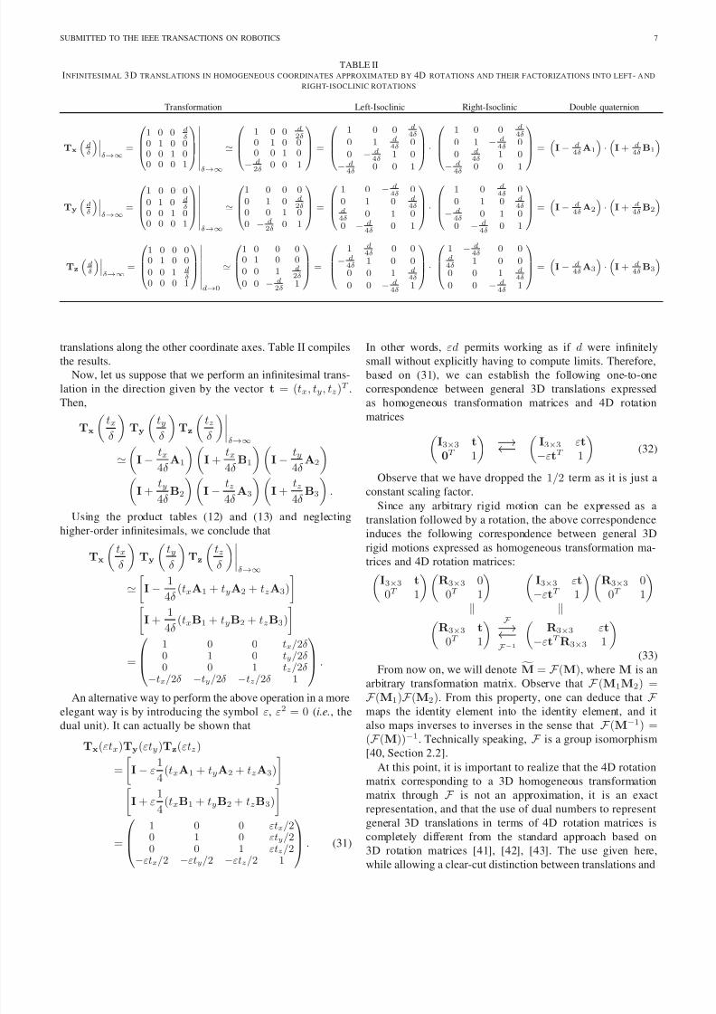
SUBMITTED TO THE IEEE TRANSACTIONS ON ROBOTICS 7
TABLE IIINFINITESIMAL 3 D TRANSLATIONS IN HOMOGENEOUS COORDINATES APPROXIMATED BY 4D ROTATIONS AND THEIR FACTORIZATIONS INTO LEFT- A ND
RIGHT-ISOCLINIC ROTATIONS
Transformation Left-Isoclinic Right-Isoclinic Double quaternion
Tx
dδ
δ→∞
=
1 0 0 dδ
0 1 0 00 0 1 00 0 0 1
δ→∞
≃
1 0 0 d2δ
0 1 0 00 0 1 0
− d2δ
0 0 1
=
1 0 0 d4δ
0 1 d4δ
0
0 − d4δ
1 0
− d4δ
0 0 1
·
1 0 0 d4δ
0 1 − d4δ
0
0 d4δ
1 0
− d4δ
0 0 1
=
I− d
4δA1
·I+ d
4δB1
Ty
dδ
δ→∞
=
1 0 0 0
0 1 0 dδ
0 0 1 00 0 0 1
δ→∞
≃
1 0 0 0
0 1 0 d2δ
0 0 1 0
0 − d2δ
0 1
=
1 0 − d4δ
0
0 1 0 d4δ
d4δ
0 1 0
0 − d4δ
0 1
·
1 0 d4δ
0
0 1 0 d4δ
− d4δ
0 1 0
0 − d4δ
0 1
=
I− d
4δA2
·I+ d
4δB2
Tz
dδ
δ→∞
=
1 0 0 00 1 0 0
0 0 1 dδ
0 0 0 1
d→0
≃
1 0 0 00 1 0 0
0 0 1 d2δ
0 0 − d2δ
1
=
1 d4δ
0 0
− d4δ
1 0 0
0 0 1 d4δ
0 0 − d4δ
1
·
1 − d4δ
0 0d4δ
1 0 0
0 0 1 d4δ
0 0 − d4δ
1
=
I− d
4δA3
·I+ d
4δB3
translations along the other coordinate axes. Table II compiles
the results.
Now, let us suppose that we perform an infinitesimal trans-
lation in the direction given by the vector t = (tx, ty, tz)T .Then,
Tx
txδ
Ty
tyδ
Tz
tzδ
δ→∞
≃
I − tx4δ
A1
I +
tx4δ
B1
I − ty
4δ A2
I + ty4δ
B2
I − tz
4δ A3
I +
tz4δ
B3
.
Using the product tables (12) and (13) and neglecting
higher-order infinitesimals, we conclude that
Tx
txδ
Ty
tyδ
Tz
tzδ
δ→∞
≃
I − 1
4δ (txA1 + tyA2 + tzA3)
I + 1
4δ (txB1 + tyB2 + tzB3)
=
1 0 0 tx/2δ 0 1 0 ty/2δ 0 0 1 tz/2δ
−tx/2δ −ty/2δ −tz/2δ 1
.
An alternative way to perform the above operation in a more
elegant way is by introducing the symbol ε, ε2 = 0 (i.e., thedual unit). It can actually be shown that
Tx(εtx)Ty(εty)Tz(εtz)
=
I − ε
1
4(txA1 + tyA2 + tzA3)
I + ε1
4(txB1 + tyB2 + tzB3)
=
1 0 0 εtx/20 1 0 εty/20 0 1 εtz/2
−εtx/2 −εty/2 −εtz/2 1
. (31)
In other words, εd permits working as if d were infinitely
small without explicitly having to compute limits. Therefore,
based on (31), we can establish the following one-to-one
correspondence between general 3D translations expressed
as homogeneous transformation matrices and 4D rotation
matrices I3×3 t
0T 1
⇄
I3×3 εt
−εtT 1
(32)
Observe that we have dropped the 1/2 term as it is just a
constant scaling factor.
Since any arbitrary rigid motion can be expressed as a
translation followed by a rotation, the above correspondence
induces the following correspondence between general 3Drigid motions expressed as homogeneous transformation ma-
trices and 4D rotation matrices:I3×3 t
0T 1
R3×3 0
0T 1
I3×3 εt
−εtT 1
R3×3 0
0T 1
R3×3 t
0T 1
F ⇄F −1
R3×3 εt
−εtT R3×3 1
(33)
From now on, we will denote M = F (M), where M is an
arbitrary transformation matrix. Observe that F (M1M2) =
F (M1)
F (M2). From this property, one can deduce that
F maps the identity element into the identity element, and italso maps inverses to inverses in the sense that F (M−1) =(F (M))−1. Technically speaking, F is a group isomorphism
[40, Section 2.2].
At this point, it is important to realize that the 4D rotation
matrix corresponding to a 3D homogeneous transformation
matrix through F is not an approximation, it is an exact
representation, and that the use of dual numbers to represent
general 3D translations in terms of 4D rotation matrices is
completely different from the standard approach based on
3D rotation matrices [41], [42], [43]. The use given here,
while allowing a clear-cut distinction between translations and
7/22/2019 Quaternions for engineers
http://slidepdf.com/reader/full/quaternions-for-engineers 8/12
SUBMITTED TO THE IEEE TRANSACTIONS ON ROBOTICS 8
rotations, provides at the same time a neat connection with
standard homogeneous transformations.
Now, the 4D rotation matrix corresponding to the translation
in the direction given by the unit vector n = (nx, ny, nz)T a
distance d, after factoring it using Cayley’s factorization, can
be expressed as:
Tn(d) = I
−ε
d
2(nxA1 + nyA2 + nzA3)
I + εd
2(nxB1 + nyB2 + nzB3)
. (34)
As with 3D rotations, the double quaternion representation
of 3D translations is also redundant because one quaternion
can be deduced from the other by exchanging Ai and Bi and
changing the sign of the dual part.
VI . KINEMATIC EQUATIONS
Consider the kinematic equation:
M0 = M1M2 · · · Mn, (35)
where Mi, i = 0, . . . , n, is an arbitrary transformation inhomogeneous coordinates. This kinematic equation can be
translated, through the mapping in (33), into a kinematic
equation fully expressed in terms of 4D rotation matrices. That
is, M0 = M1M2 · · ·Mn. (36)
Then, using Cayley’s factorization, we obtainML0MR
0 = ML1MR
1ML
2MR
2 · · ·MLnMR
n . (37)
Therefore, using the properties of left- and right-isoclinic
rotations, we conclude that
ML
0
=ML
1 ML
2 · · ·ML
n
, (38)MR0 =MR
1MR
2 · · ·MRn . (39)
Each rotation matrix in (38), or (39), can readily be
interpreted as a quaternion if expressed in the basis
{I, A1, A2, A3}, or {I, B1, B2, B3}. Moreover, as we have
already seen, any of these two equations can be obtained from
the other by exchanging Ai and Bi and changing the sign of
the dual symbol.
Although translations and rotations provide the basic build-
ing blocks of any kinematic equation, in many applications it
is interesting to have a more compact expression for motions
combining a rotation about an axis and a translation in the
direction given by the same axis (i.e., screw motions). Indeed,if we define
S = Rn(θ)Tn(d), (40)
thenSR =
cos
θ
2
− ε
d
2 sin
θ
2
I
+
sin
θ
2
+ ε
d
2 cos
θ
2
(nxB1 + nyB2 + nzB3).
(41)
Since all powers greater or equal to two of ε vanish, the
Taylor expansion of f (a + εb) about a yields f (a) + εbf ′(a).
As a consequence, sin(a + εb) = sin a + εb cos a and cos(a +εb) = cos a − εb sin a [43, p. 3]. Therefore, (41) can be more
compactly expressed as:
SR = cos
θ
2
I +sin
θ
2
(nxB1 + nyB2 + nzB3), (42)
where θ = θ + εd. The dual quaternion (42) is undoubtedly
a much more compact representation of a screw motionthan the expansion of (40). Thus, it is not surprising that
dual quaternions defining successive screw displacements are
introduced to simplify the structure of the design equations in
the synthesis of mechanisms [29].
The screw displacement given by (42) is not general as the
rotation axis passes through the origin. The general form is
derived as an example in the next section.
VII. EXAMPLES
The following examples illustrate different aspects on how
to operate with the presented twofold matrix-quaternion for-
malism.
A. Derivation of the sandwich formula
It is straightforward to prove that, if q = C p, where C is
an arbitrary rotation matrix in homogeneous coordinates and
p a unit vector, then
Rq(θ) = C Rp(θ) CT . (43)
If we substitute (30) in (43), set θ = π, and separate left- and
right-isoclinic rotations, we obtain
(q xA1 + q yA2 + q zA3) = CL( pxA1 + pyA2 + pzA3)(CL)T
(44)
and
(q xB1 + q yB2 + q zB3) = CR( pxB1 + pyB2 + pzB3)(CR)T
(45)
respectively.
Observe that either (44) or (45), after expressing CR and
CL in quaternion form according to (2) and (3), respectively,
is the well-known quaternion sandwich formula used to rotate
vectors. It is interesting to observe the number of pages de-
voted to the derivation of this formula in current textbooks [4,
pp. 127-134], [7], and the existence of recent papers essentially
devoted to its justification [8], while its derivation using the
proposed twofold matrix-quaternion formulation seems much
easier, at least for those used to work with homogenous
transformations.
B. Approximating dual quaternions by double quaternions
Let us suppose that we need to obtain the quaternion
representation of the following transformation in homogeneous
coordinates
M = Tx(4)Ty(−3)Tz(7)Ry
π
2
Rz
π
2
=
0 0 1 41 0 0 −30 1 0 70 0 0 1
. (46)
7/22/2019 Quaternions for engineers
http://slidepdf.com/reader/full/quaternions-for-engineers 9/12
SUBMITTED TO THE IEEE TRANSACTIONS ON ROBOTICS 9
The 4D rotation matrix resulting from the mapping in (33)
is:
M =
0 0 1 4ε1 0 0 −3ε0 1 0 7ε
3ε −7ε −4ε 1
. (47)
Cayley’s factoring of this matrix into a left- and right-isoclinic
rotation matrix, using the procedure given in the appendix,yields:
ML =
0.5 + 2ε −0.5 + 3.5ε 0.5 −0.5 − 1.5ε0.5 − 3.5ε 0.5 + 2ε −0.5 − 1.5ε −0.5−0.5 0.5 + 1.5ε 0.5 + 2ε −0.5 + 3.5ε
0.5 + 1.5ε 0.5 0.5 − 3.5ε 0.5 + 2ε
=(0.5 + 2ε)I + (0.5 + 1.5ε)A1 + 0.5A2 + (0.5 − 3.5ε)A3
(48)
and
MR
=0.5 − 2ε −0.5 − 3.5ε 0.5 0.5 − 1.5ε
0.5 + 3.5ε 0.5−
2ε −
0.5 + 1.5ε 0.5−0.5 0.5 − 1.5ε 0.5 − 2ε 0.5 + 3.5ε
−0.5 + 1.5ε −0.5 −0.5 − 3.5ε 0.5 − 2ε
=(0.5 − 2ε)I + (0.5 − 1.5ε)B1 + 0.5B2 + (0.5 + 3.5ε)B3,(49)
respectively. Hence,
M = MLMR =[(0.5 + 2ε)I + (0.5 + 1.5ε)A1
+ 0.5A2 + (0.5 − 3.5ε)A3]
[(0.5 − 2ε)I + (0.5 − 1.5ε)B1
+ 0.5B2 + (0.5 + 3.5ε)B3].
This double quaternion representation is redundant as onequaternion can be deduced from the other by exchanging Ai
and Bi and changing the sign of the dual part. Thus, either
the dual quaternion (48) or (49) unambiguously represents the
transformation (46).
The rotation matrix M is an exact representation of M, it
is not an approximation. Alternatively, if we are not interested
in using dual numbers, we can approximate M by
M =
0 0 1 4/δ 1 0 0 −3/δ 0 1 0 7/δ
3/δ −
7/δ −
4/δ 1
. (50)
where δ is a scaling factor. M is closer to a 4D rotation
matrix as δ tends to infinity (it can be verified that det(M ) =
1 − 5/δ 2). This is the approach pioneered in [44] and [45]
to approximate 3D homogeneous transformations by 4D rota-
tion matrices and used, for example, in [23] in dimensional
synthesis, or in [46] to solve the inverse kinematics of a
6R robot. This kind of approximation introduces a tradeoff
between numerical stability and accuracy of the approximation
(see [45] for details). If we factor M into a left- and a right-
isoclinic rotation, with δ = 100, we obtain:
M L
=
0.5204 −0.4632 0.4996 −0.51520.4632 0.5204 −0.5152 −0.4996
−0.4996 0.5152 0.5204 −0.46320.5152 0.4996 0.4632 0.5204
= 0.5204I + 0.5152A1 + 0.4996A2 + 0.4632A3 (51)
and
M R
=
0.4804 −0.5332 0.4996 0.48520.5332 0.4804 −0.4852 0.4996
−0.4996 0.4852 0.4804 0.5332−0.4852 −0.4996 −0.5332 0.4804
= 0.4804I + 0.4852B1 + 0.4996B2 + 0.5332B3.
(52)
Hence, M LM R
can be used as an approximation of
M by properly scaling the translations. This approximate
double quaternion representation of M is not redundant as
one quaternion cannot be deduced from the other.
C. Computation of screw parameters
Chasles’ theorem states that the general spatial motion of
a rigid body can be produced a rotation about an axis and a
translation along the direction given by the same axis. Such
a combination of translation and rotation is called a general
screw motion [47]. In the definition of screw motion, a positive
rotation corresponds to a positive translation along the screw
axis by the right-hand rule.
q p
n
θ
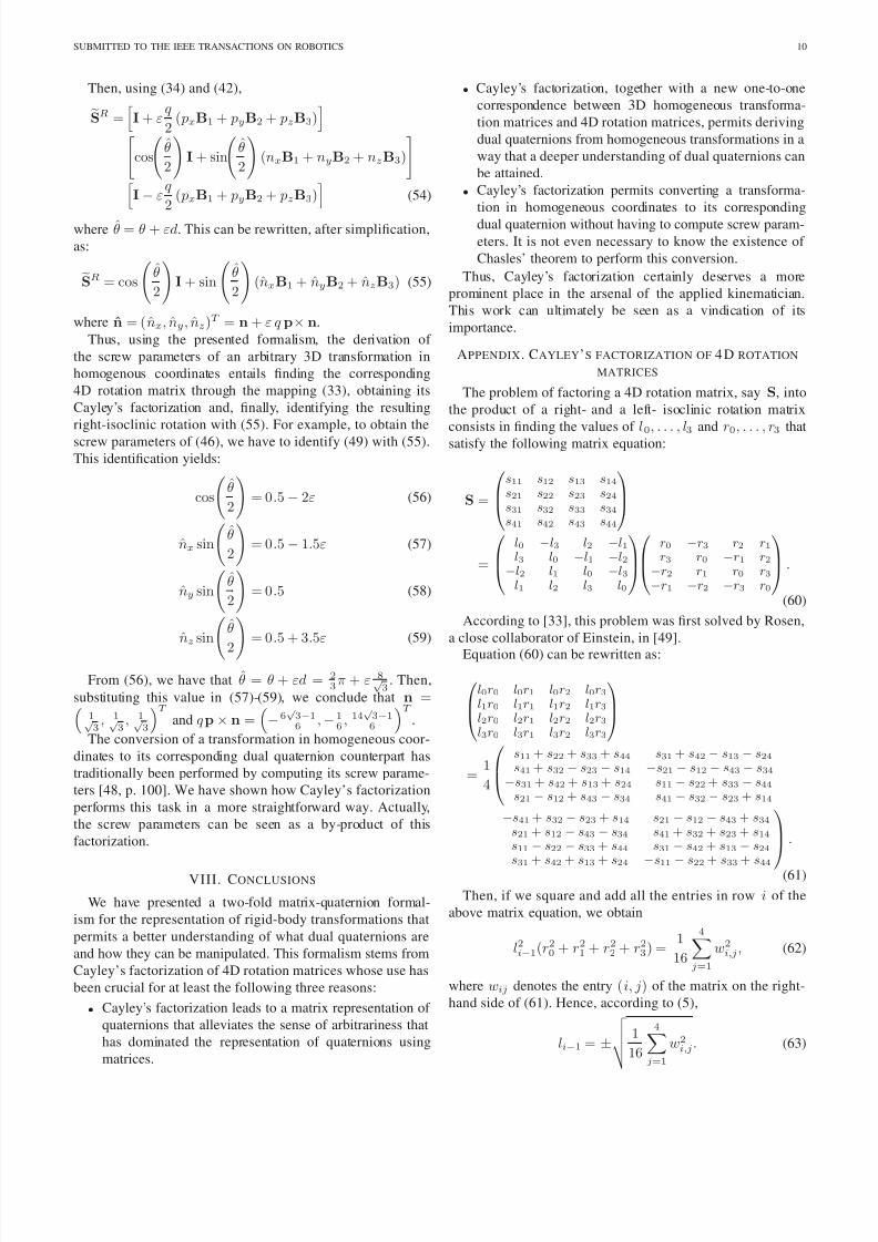
Fig. 1. Geometrix parameters used to describe a general screw motion.
In Fig. 1, a screw axis is defined by n = (nx, ny, nz)T , a
unit vector defining its direction, and q p, the position vector
of a point lying on it, where p = ( px, py, pz)T is also
a unit vector. The angle of rotation θ and the translational
distance d are called the screw parameters. These screw
parameters together with the screw axis completely define the
general displacement of a rigid body. In terms of homogeneous
transformations, in a way similar to (43), this can be expressed
as:
S = Tp(q )Rn(θ)Tn(d)Tp(−q ) (53)
7/22/2019 Quaternions for engineers
http://slidepdf.com/reader/full/quaternions-for-engineers 10/12
SUBMITTED TO THE IEEE TRANSACTIONS ON ROBOTICS 10
Then, using (34) and (42),SR =
I + εq
2 ( pxB1 + pyB2 + pzB3)
cos
θ
2
I + sin
θ
2
(nxB1 + nyB2 + nzB3)
I − ε
q
2 ( pxB1 + pyB2 + pzB3)
(54)
where θ = θ + εd. This can be rewritten, after simplification,
as:
SR = cos
θ
2
I + sin
θ
2
(nxB1 + nyB2 + nzB3) (55)
where n = (nx, ny, nz)T = n + ε q p× n.
Thus, using the presented formalism, the derivation of
the screw parameters of an arbitrary 3D transformation in
homogenous coordinates entails finding the corresponding
4D rotation matrix through the mapping (33), obtaining its
Cayley’s factorization and, finally, identifying the resulting
right-isoclinic rotation with (55). For example, to obtain the
screw parameters of (46), we have to identify (49) with (55).
This identification yields:
cos
θ
2
= 0.5 − 2ε (56)
nx sin
θ
2
= 0.5 − 1.5ε (57)
ny sin
θ
2
= 0.5 (58)
nz sinθ
2 = 0.5 + 3.5ε (59)
From (56), we have that θ = θ + εd = 2
3π + ε 8√
3. Then,
substituting this value in (57)-(59), we conclude that n = 1√ 3
, 1√ 3
, 1√ 3
T and q p × n =
− 6
√ 3−16
, − 1
6, 14
√ 3−16
T .
The conversion of a transformation in homogeneous coor-
dinates to its corresponding dual quaternion counterpart has
traditionally been performed by computing its screw parame-
ters [48, p. 100]. We have shown how Cayley’s factorization
performs this task in a more straightforward way. Actually,
the screw parameters can be seen as a by-product of this
factorization.
VIII. CONCLUSIONS
We have presented a two-fold matrix-quaternion formal-
ism for the representation of rigid-body transformations that
permits a better understanding of what dual quaternions are
and how they can be manipulated. This formalism stems from
Cayley’s factorization of 4D rotation matrices whose use has
been crucial for at least the following three reasons:
• Cayley’s factorization leads to a matrix representation of
quaternions that alleviates the sense of arbitrariness that
has dominated the representation of quaternions using
matrices.
• Cayley’s factorization, together with a new one-to-one
correspondence between 3D homogeneous transforma-
tion matrices and 4D rotation matrices, permits deriving
dual quaternions from homogeneous transformations in a
way that a deeper understanding of dual quaternions can
be attained.
• Cayley’s factorization permits converting a transforma-
tion in homogeneous coordinates to its corresponding
dual quaternion without having to compute screw param-
eters. It is not even necessary to know the existence of
Chasles’ theorem to perform this conversion.
Thus, Cayley’s factorization certainly deserves a more
prominent place in the arsenal of the applied kinematician.
This work can ultimately be seen as a vindication of its
importance.
APPENDIX. CAYLEY’S FACTORIZATION OF 4 D ROTATION
MATRICES
The problem of factoring a 4D rotation matrix, say S, into
the product of a right- and a left- isoclinic rotation matrix
consists in finding the values of l0, . . . , l3 and r0, . . . , r3 that
satisfy the following matrix equation:
S =
s11 s12 s13 s14s21 s22 s23 s24s31 s32 s33 s34s41 s42 s43 s44
=
l0 −l3 l2 −l1l3 l0 −l1 −l2
−l2 l1 l0 −l3l1 l2 l3 l0
r0 −r3 r2 r1
r3 r0 −r1 r2−r2 r1 r0 r3−r1 −r2 −r3 r0
.
(60)
According to [33], this problem was first solved by Rosen,
a close collaborator of Einstein, in [49].
Equation (60) can be rewritten as:l0r0 l0r1 l0r2 l0r3l1r0 l1r1 l1r2 l1r3l2r0 l2r1 l2r2 l2r3l3r0 l3r1 l3r2 l3r3
=
1
4
s11 + s22 + s33 + s44 s31 + s42 − s13 − s24s41 + s32 − s23 − s14 −s21 − s12 − s43 − s34
−s31 + s42 + s13 + s24 s11 − s22 + s33 − s44s21 − s12 + s43 − s34 s41 − s32 − s23 + s14
−s41 + s32 − s23 + s14 s21 − s12 − s43 + s34s21 + s12 − s43 − s34 s41 + s32 + s23 + s14s11 − s22 − s33 + s44 s31 − s42 + s13 − s24s31 + s42 + s13 + s24
−s11
−s22 + s33 + s44
.
(61)
Then, if we square and add all the entries in row i of the
above matrix equation, we obtain
l2i−1(r20 + r21 + r22 + r23) = 1
16
4j=1
w2i,j, (62)
where wij denotes the entry (i, j) of the matrix on the right-
hand side of (61). Hence, according to (5),
li−1 = ± 1
16
4j=1
w2i,j. (63)
7/22/2019 Quaternions for engineers
http://slidepdf.com/reader/full/quaternions-for-engineers 11/12
SUBMITTED TO THE IEEE TRANSACTIONS ON ROBOTICS 11
Therefore, assuming that li−1 = 0, which is always true for
at least one value of i according to (4), the entries of the
right-isoclinic matrix can be obtained as follows:
rj−1 = wi,j
li−1. (64)
Now, if we take a value of j for which rj−1 = 0, all other
entries of the left-isoclinic matrix, besides that obtained in
(63), can be obtained as follows:
lk−1 = wk,j
rj−1. (65)
Observe that we have two possible solutions for the fac-
torization depending on the sign chosen for the square root in
(63). This simply says that the factorization of S into isoclinic
rotations can either be expressed as SLSR or (−SL)(−SR).
In other words, Cayley’s factorization is unique up to a sign
change. The consequence of this fact is that quaternions
provide a double covering of the space of rotations.
ACKNOWLEDGMENT
The author would like to thank the anonymous reviewers for
their extremely detailed comments and suggestions to improve
the quality of the paper.
REFERENCES
[1] W.R. Hamilton, “On Quaternions or a new system of imaginaries inalgebra,” Philosophical Magazine, Vol. 25, pp. 489-495, 1844.
[2] A.M. Bork, “Vectors versus quaternions. The letters in Nature,” American Journal of Physics, Vol. 34, No. 3, pp. 202-211, 1966.
[3] A. C. Robinson, “On the use of quaternions in simulation of rigid-bodymotion,” WADC technical report , 1958.
[4] J.B. Kuippers, Quaternions and Rotation Sequences, Princeton UniversityPress, Princeton, 1999.
[5] J.D. Foley and A. Van Dam, Fundamentals of Interactive Computer
Graphics, Addison-Wesley Publishing Co., 1982.[6] M.D. Shuster, “The nature of the Quaternion,” The Journal of the
Astronautical Sciences, Vol. 56, No. 3, pp. 359-371, 2008.[7] R. Goldman, Rethinking Quaternions. Theory and Computation, Morgan
and Claypool Publishers, 2010.[8] J. McDonald, “Teaching quaternions is not complex,” Computer Graphics
Forum, Vol. 29, No. 8, pp. 2447-2455, 2010.[9] S.L. Altmann, “Hamilton, Rodrigues, and the quaternion scandal,” Math-
ematics Magazine, Vol. 62, No. 5, pp. 291-308, 1989.[10] W.R. Hamilton, Lectures on Quaternions, Hodges & Smith, Dublin,
1853.[11] M.D. Shuster, “A Survey of attitude representations,” The Journal of the
Astronautical Sciences, Vol. 41, No. 4, pp. 439-517, 1993.[12] J. Pujol, “Hamilton, Rodrigues, Gauss, Quaternions, and Rotations: a
Historical Reassessment,” Communications in Mathematical Analysis,Vol. 13, No. 2, pp. 1-14, 2012.
[13] A. Cayley, “On certain results relating to quaternions,” Philosophical
Magazine, Vol. 26, pp. 141-145, 1845.[14] A. Cayley, “Recherches ulterieures sur les determinants gauches,” The
Collected Mathematical Papers Of Arthur Cayley, article 137, p. 202-215,Cambridge Uniniversity Press, 1891.
[15] J.L.Weiner and G.R. Wilkens, “Quaternions and rotations in E 4,” The American Mathematical Monthly, Vol. 112, No. 1, pp. 69-76, 2005.
[16] L. van Elfrinkhof, “Eene eigenschap van de orthogonale substitutievan de vierde orde,” Handelingen van het zesde Nederlandsch Natuur-en Geneeskundig Congres (Acts of the sixth Dutch nature and medicalcongress), pp. 237-240, Delft, 1897.
[17] J.E. Mebius, Applications of Quaternions to Dynamical Simulation,Computer Graphics and Biomechanics, Ph.D. Thesis, Delft Universityof Technology, 1994.
[18] W.K. Clifford, Collected Mathematical Papers, Edited by R. Tucker,Macmillan and co., London, 1882. Reprinted in 1968 by Chelsea Pub-lishing Company, New York.
[19] J. Rooney, “William Kingdon Clifford (1845-1879),” In: Ceccarelli,Marco ed. Distinguished figures in mechanism and machine science: Their contributions and legacies. History of mechanism and machine science,Volume 1. Dordrecht, Netherlands: Springer, pp. 79-116.
[20] I.M. Yaglom, Complex Numbers in Geometry, Academic Press, NewYork, 1968.
[21] I.L. Kantor and A.S. Solodovnikov, Hypercomplex numbers, Berlin, NewYork: Springer-Verlag, 1989.
[22] A. Buchheim, “A memoir on biquaternions,” American Journal of Mathematics, Vol. 7, No. 4 , pp. 293-326, 1885.
[23] J.M. McCarthy and S. Ahlers, “Dimensional synthesis of robots usinga double quaternion formulation of the workspace,” 9th InternationalSymposium of Robotics Research, ISRR’99, pp 1-6, 1999.
[24] J. Selig, Geometrical Methods in Robotics, Springer, New York, 1996.[25] L. Dorst and S. Mann, “Geometric Algebra: a computational framework
for geometrical applications (Part 1),” IEEE Computer Graphics and Applications, Vol. 22, No. 3, pp. 24-31, 2002.
[26] A.T. Yang and F. Freudenstein, “Application of dual-number quaternionalgebra to the analysis of spatial mechanisms,” Transactions of the ASME,
Journal of Applied Mechanics E , Vol. 31, No. 2, pp. 300-308, 1964.[27] J.M. McCarthy, Introduction to Theoretical Kinematics, The MIT Press,
1990.[28] J. Angeles, “The application on dual algebra to kinematic analysis,”
Computational Methods in Mechanical Systems, NATO ASI Series (ed.J. Angeles and E. Zakhariev), Springer, Berlin, 1998.
[29] A. Perez-Gracia, Dual Quaternion Synthesis of Constrained RoboticSystems, PhD dissertation, University of California, Irvine, 2003.
[30] A.J. Hanson, Visualizing Quaternions, Morgan Kaufmann, 2006.[31] C.Y. Hsiung and G.Y. Mao, Linear Algebra, Allied Publishers, 1998.[32] L. Pertti, Clifford algebras and spinors, Cambridge University Press,
2001.[33] F.L. Hitchcock, “Analysis of rotations in euclidean four-space by
sedenions,” Journal of Mathematics and Physics, Univerisity of Mas-sachusetts, Vol. 9, No. 3, pp. 188-193, 1930.
[34] G. Juvet, “Les rotations de l’espace Euclidien a quatre dimensions, leurexpression au moyen des nombres de Clifford et leurs relations avec latheorie des spineurs,” Commentarii mathematici Helvetici, Vol. 8, pp.264-304, 1936.
[35] P. Corke, Robotics, Vision and Control: Fundamental Algorithms in MATLAB, Springer, 2011.
[36] J.J. Craig, Introduction to robotics: Mechanics and control, ThirdEdition, Prentice Hall, 2004.
[37] Q.J. Ge, A. Varshney, J.P. Menon, and C-F. Chang, “Double quater-nions for motion interpolation,” Proc. of the 1998 ASME ASME Design
Manufacturing Conference, Atlanta, GA, Paper No. DETC98/DFM-5755,1998.
[38] P. Larochelle, A. Murray, and J. Angeles, “A distance metric for finitesets of rigid-body displacements via the polar decomposition,” ASME
Journal of Mechanical Design, Vol. 129, No. 8, pp. 883-886, 2007.[39] D.W. Eggert, A. Lorusso, and R.B. Fisher, “Estimating 3-D rigid body
transformations: a comparison of four major algorithms,” Machine Visionand Applications, Vol. 9, No. 5, pp. 272-290, 1997.
[40] J. Stillwell, Naive Lie Theory, Springer, 2008.[41] G.R. Veldkamp, “On the use of dual numbers, vectors and matrices in
instantaneous, Spatial Kinematics,” Mechanism and Machine Theory, Vol.11, pp. 141-156, 1976.
[42] G.R. Pennock and A.T. Yang, “Application of dual-number matrices tothe inverse kinematics problem of robot manipulators,” ASME Journal of
Mechanisms, Transmissions, and Automation in Design, Vol. 107, No. 2,201 (8 pages), 1985.
[43] I.S. Fischer, Dual-Number Methods in Kinematics, Statics and Dynam-
ics, CRC Press, 1999.[44] P. Larochelle and J.M. McCarthy, “Planar motion synthesis using an
approximate bi-invariant metric,” ASME J. Mechanical Design, Vol. 117,pp. 646-651, 1995.
[45] K.R. Etzel and J.M. McCarthy, “A metric for spatial displacement usingbiquaternions on SO(4),” International Conference on Robotics and
Automation, Vol. 4, pp. 3185-3190, 1996.[46] S. Qiao, Q. Liao, S. Wei and H-J. Su, “Inverse kinematic analysis of the
general 6R serial manipulators based on double quaternions,” Mechanismand Machine Theory, Vol. 45, pp. 193-199, 2010.
[47] J.K. Davidson and K.H. Hunt, Robots and Screw Theory: Applications
of Kinematics and Statics to Robotics, Oxford Univ Press, Oxford, 2004.[48] J. Angeles, Fundamentals of Robotic Mechanical Systems: Theory,
Methods, and Algorithms, Springer, 2006.[49] N. Rosen, “Note on the general Lorentz transformation,” Journal of
Mathematics and Physics, Vol. 9, pp. 181-187, 1930.

7/22/2019 Quaternions for engineers
http://slidepdf.com/reader/full/quaternions-for-engineers 12/12
SUBMITTED TO THE IEEE TRANSACTIONS ON ROBOTICS 12
Federico Thomas (M’06) received the Telecom-munications Engineering degree in 1984 and thePh.D. degree in computer science in 1988, both fromthe Technical University of Catalonia, Barcelona,Spain. He is currently a Research Professor at theSpanish Scientific Research Council, Instituto deRobotica e Informatica Industrial, Barcelona. Hisresearch interests include geometry and kinematicswith applications to robotics. Prof. Thomas was anAssociate Editor of the IEEE TRANSACTIONS ON
ROBOTICS.
![Quadratic Split Quaternion Polynomials: …...been done for quaternions in [6] and for split quaternions in [2]. Results for generalized quaternions, including split quaternions, can](https://img.pdfslide.us/doc/110x75/5ea3ed9b0e257f05c666f8d7/quadratic-split-quaternion-polynomials-been-done-for-quaternions-in-6-and.jpg)