Quarterly Journal of the Business Valuation … VALUATION REVIEW —Published quarterly by the Business Valuation Committee of the American Society of Appraisers. TM Editor:

Published by the American Society of Appraisers Copyright © 2016 American Society of Appraisers Qu

arte

rly Jo

urna

l of t

he B

usin

ess V

alua

tion

Com

mitt

ee o

f the

Am

erica

n So

ciety

of A

ppra

isers

Volume 35

Issue 3

Fall 2016

77 Editor’s Column Dan McConaughy, PhD, ASA

78 AMERICAN SOCIETY OF APPRAISERS: Business Valuation Committee Special Topics Paper #1: Use of Offers as Indications of Value in the Market Approach

81 Estimating Discounts for Lack of Marketability: Understanding Alternative Approaches—Put Options Versus Monetizing an Option Collar Jay E. Fishman, FASA, and Bonnie O’Rourke, ASA

86 EBITDA Single-Period Income Capitalization for Business Valuation Z. Christopher Mercer, FASA, CFA, ABAR

103 Two Theories of Control Eric Sundheim, BA, ASA, and Jordan Sundheim, MA, BA

112 From the Chair William A. Johnston, ASA

Business Valuation Review – Fall 2016

The Business Valuation Committee

Chair William A. Johnston, ASA – Empire Valuation Consultants, LLC

Vice Chair Jeffrey S. Tarbell, ASA – Houlihan Lokey

Secretary Erin Hollis, ASA – Marshall & Stevens, Inc.

Treasurer Kenneth J. Pia, Jr., ASA – Meyers, Harrison & Pia, LLC

Past Chair Robert B. Morrison, ASA – Morrison Valuation & Forensic Services, LLC

Members At-Large Gregory Ansel, ASA – Financial Strategies Consulting Group LLC Arlene Ashcraft, ASA – Columbia Financial Advisors, Inc. KC Conrad, ASA – American Business Appraisers Matthew R. Crow, ASA – Mercer Capital Nancy M. Czaplinski, ASA – Duff & Phelps Erin Hollis, ASA – Marshall & Stevens, Inc. Bruce Johnson, ASA – Munroe, Park & Johnson, Inc. Curtis T. Johnson, ASA – Ernst & Young Timothy Meinhart, ASA – Willamette Management Associates Susan Saidens, ASA – SMS Valuation & Financial Forensics Ronald L. Seigneur, ASA – Seigneur Gustafson LLP Gary R. Trugman, ASA – Trugman Valuation Associates, Inc. Mark Zyla, ASA – Acuitas, Inc.

Ex Officio James O. Brown, ASA – Perisho Tombor Brown, PC R. Chris Rosenthal, ASA – Ellin & Tucker Linda B. Trugman, ASA – Trugman Valuation Associates, Inc.

Emeritus Jay E. Fishman, FASA – Financial Research Associates Shannon P. Pratt, FASA – Shannon Pratt Valuations, LLC

HQ Advisor Bonny Price

BUSINESS VALUATION REVIEW TM —Published quarterly by the Business Valuation Committee of the American Society of Appraisers. Editor: Daniel L. McConaughy, PhD, ASA. Managing Editor: Chris Brower, [email protected].

INTERNATIONAL STANDARD SERIAL NUMBER—The Library of Congress, National Serials Data Pro = ISSN 0897-1781.SUBSCRIPTION RATES—PRINT AND ELECTRONIC ACCESS: Members of American Society of Appraisers-$60 if paid with annual dues;

all others—$140 per year. Direct any questions and/or subscription changes to Bonny F. Price (703) 733-2110 or [email protected]—Authors should submit their articles (including charts, graphs, pictures, etc.) for publication in Business Valuation Review ©

at http://www.editorialmanager.com/bvr/. Follow the new user registration login instructions, at the Register Now hotlink. Since we use a double-blind peer review system, authors should provide the author’s name (as it would appear if published), and a short one-paragraph description of professional activities when completing the registration process. An abstract should appear at the beginning of the paper submitted for review. Authors are asked to not submit manuscripts currently under review by other publications or that have been published elsewhere. All manuscripts are reviewed by the Editorial Review Board and may be accepted, rejected, or returned for additional work. Editor’s notes may be included with the printing of accepted articles. All authors will be so notified. No manuscripts will be returned, and no critiques or reasons for rejection will be given for material not selected for publication.

CLASSIFIED ADS—Accepted for publication in one issue only and should reach the Publisher no later than the 10th of the month prior to publication. Rates: full page—$500, 2/3 page—$375, 1/2 page—$300, 1/3 page—$200, 1/4 page—$150. Payable in U.S. funds. Direct any questions to Bonny F. Price (703) 733-2110 or [email protected]

LETTERS TO THE EDITOR & COMMENTS—Letters from readers are encouraged on any valuation subject. BVR reserves the right to edit letters for length, taste and/or clarity. No guarantee of publica tion is given. Please direct critique or comments to the Editor. All Letters to the Editor should be submitted at http://www.editorialmanager.com/bvr/.

STATEMENTS & OPINIONS—Statements expressed herein by the authors and contributors to Business Valuation Review are their own and not necessarily those of the American Society of Appraisers or its Business Valuation Committee.

Copyright, © American Society of Appraisers—2016All rights reserved. For permission to reproduce in whole or part, and for quotation privilege, contact International Headquarters of ASA. Neither the Society nor its Editor accepts responsibility for statements or opinions advanced in articles appearing herein, and their appearance does not necessarily constitute an endorsement.

EditorDaniel L. McConaughy, PhD, ASA

California State University Northridge

Managing EditorChris Brower

Lawrence, Kansas

Business ManagerJames O. Brown, ASA Campbell, California

ReviewersVincent Covrig*, PhD, CFA

Los Angeles, California

Roxanne Cheng*, ASA Pasadena, California

Bob Dohmeyer, ASA Frisco, Texas

Tiago Duarte-Silva Boston, Massachusetts

John D. Finnerty, PhD New York, New York

Roger Grabowski*, FASA Chicago, Illinois

Alan Imberman, MBA, CFA Dallas, Texas

William Kennedy*, PhD Boston, Massachusetts

Eric Nath, ASA San Francisco, California

Michael Vitti, BS Morristown, New Jersey

*Editorial Board Member

Editors EmeritusJames H. Schilt, ASA (1982–2001)

San Francisco, California

Jay E. Fishman, FASA (2002–2007) Bala Cynwyd, Pennsylvania

Roger J. Grabowski, FASA (2008–2012) Chicago, Illinois

Publishers EmeritusJohn E. Bakken, FASA (1982–2003)

Granby, Colorado

Ralph Arnold, III, ASA (2004–2007) Portland, Oregon

BVR Editorial Review Board

© 2016, American Society of Appraisers

EBITDA Single-Period Income Capitalization for BusinessValuation

Z. Christopher Mercer, FASA, CFA, ABAR

This article begins with a discussion of EBITDA, or earnings before interest, taxes,

depreciation, and amortization. The focus on the EBITDA of private companies is

almost ubiquitous among business appraisers, business owners, and other market

participants. The article then addresses the relationship between depreciation (and

amortization) and EBIT, or earnings before interest and taxes, as one measure of

relative capital intensity. This relationship, which is termed the EBITDA Depreciation

Factor, is then used to convert debt-free pretax (i.e., EBIT) multiples into corresponding

multiples of EBITDA. The article presents analysis that illustrates why, in valuation

terms (i.e., expected risk, growth, and capital intensity), the so-called pervasive rules of

thumb suggesting that many companies are worth 4.03 to 6.03 EBITDA, plus or minus,

exhibit such stickiness. The article suggests a technique based on the adjusted capital

asset pricing model whereby business appraisers and market participants can

independently develop EBITDA multiples under the income approach to valuation.

Finally, the article presents private and public company market evidence regarding the

EBITDA Depreciation Factor, which should facilitate further investigation and analysis.

What is EBITDA?1

EBITDA is an acronym for earnings before interest,

taxes, depreciation, and amortization. It is important

because, as we will see, EBITDA is the initial source of

cash flow for all reinvestment in a business and for all

returns to shareholders.2

Why is EBITDA such a ubiquitous term, particularly in

the market for private businesses and in their valuation? It

is not because EBITDA is uniquely capitalizable, but

because it is the most comparable measure of income

across a broad range of private (and public) companies.

Think about EBITDA:

� EBITDA neutralizes tax differences across private

companies, because it is a measure of cash flow

before taxes are considered.� EBITDA neutralizes capital structure differences.

Since EBITDA measures cash flow before interest

expense, buyers consider their own financing

structures, regardless of the financing of sellers.3

� EBITDA neutralizes accounting differences. Depre-

ciation can be straight line or accelerated, and

EBITDA captures the difference in measuring cash

flow. In addition, EBITDA captures differences in

amortization, or differences between companies that

build out their growth or purchase it.

EBITDA is, then, a ‘‘lowest-common-denominator’’way to express relative value. It can be used to compare

different companies at a point in time or over time or

specific companies over time.

Keep in mind, however, that despite the pervasiveness

of vocabulary among business appraisers and market

participants, buyers do not buy EBITDA. They buy cash

Z. Christopher Mercer, FASA, CFA, ABAR, isfounder and chief executive officer of Mercer Capital,a national business valuation firm.

1I would like to thank Travis Harms, CPA/ABV, CFA, senior vicepresident at Mercer Capital, for reviewing several drafts of this article.Any issues or problems with the article, however, fall to me.2Early readers of this article are of two minds when it comes to the followingfairly lengthy discussion of EBITDA. I have taken a ‘‘by-the-line’’ approachto explaining the concepts in the article, which adds to the length as well asclarity, I hope. The early readers either think the discussion is interesting andenlightening, or they think it is too long and too obvious. Based on more thanthirty-five years in valuing businesses and dealing with business owners,accountants, attorneys, judges, financial planners and other referral sources,and other appraisers as well, nothing is too obvious. Further, as noted in thearticle, very little has been written about EBITDA in the appraisal literature.As readers will see, even with a concept so ‘‘obvious’’ as EBITDA, there aremany nuances that must be considered when analyzing EBITDA and itsimpact on value.

3EBITDA may not control for differences in capital structure related tocapital leases versus operating leases. If operating leases are significant,the analyst may employ a different analysis and may employ a differentvaluation method.

Page 86 � 2016, American Society of Appraisers

Business Valuation Review

Volume 35 � Number 3

� 2016, American Society of Appraisers

flow. A review of current valuation texts provides little

insight into EBITDA, how to analyze it, or how to

capitalize it. The entire discussion of EBITDA in five

valuation texts is summarized below:

1. Valuing a Business, 5th ed.4 This text mentions

possibly capitalizing EBITDA in calculating the

terminal value for discounted cash flow valuation

methods, but it indicates a preference for using the

Gordon model.

2. Financial Valuation: Applications and Models, 3rd

ed.5 This volume mentions using guideline market

data to capitalize EBITDA for terminal value

determinations in discounted cash flow methods,

but it suggests that appraisers use the Gordon model.

Hitchner notes: ‘‘Using concepts such as EBIT

[earnings before interest and taxes] and EBITDA

can be useful because they can reflect the economics

of the business better than net income and cash flow,

which are very much influenced by both the

company’s tax planning and its choice of capital

structure.’’ He then mentions advantages of EBIT and

EBITDA because they reflect the operations of the

business and exclude nonoperating, financial (capital

structure), and tax planning (depreciation policies)

aspects that are part of net income. Because of

variances in these factors across companies, EBITDA

may be preferable in some instances to net income. It

is noted that net operating income before replacement

reserves in real estate is similar in concept to

EBITDA. The final mention pertains to the invested

capital/EBITDA multiple, where the text notes that

public EBITDA multiples for hospitals are often

considerably higher than relevant multiples for

individual hospitals.

3. Understanding Business Valuation: A PracticalGuide to Valuing Small to Medium Sized Business-es.6 The Trugman book does not mention EBITDA,

but it does briefly discuss EBIT.

4. PPC’s Guide to Business Valuations. EBITDA is

not found in the index, and I did not find any

discussion of the topic.

5. Valuation: Measuring and Managing the Value ofCompanies, 4th ed.7 The most extensive discussion

of EBITDA and EBITDA multiples is found in

chapter 12 of the McKinsey & Company book. The

chapter focuses more on EBITA (earnings before

interest, taxes, and amortization) than on EBITDA.

The chapter provides a formula for deriving

enterprise value/EBITA multiples that allows for

the substitution of an ROIC (return on invested

capital) that is different than the weighted average

cost of capital (WACC) for a business being valued.

The chapter discusses best practices for using

multiples, enterprise value (as discussed in this

article), and alternative multiples like enterprise

value/sales.

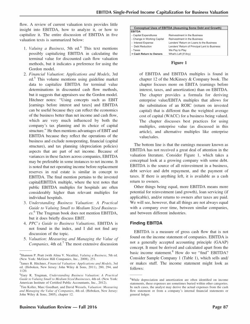
The bottom line is that the earnings measure known as

EBITDA has not received a great deal of attention in the

valuation literature. Consider Figure 1, which takes a

conceptual look at a growing company with some debt.

EBITDA is the source of all reinvestment in a business,

debt service and debt repayment, and the payment of

taxes. If there is anything left, it is available as a cash

return to owners.

Other things being equal, more EBITDA means more

potential for reinvestment (and growth), loan servicing (if

applicable), and/or returns to owners after taxes are paid.

We will see, however, that all things are not always equal

with a company over time, between similar companies,

and between different industries.

Finding EBITDA

EBITDA is a measure of gross cash flow that is not

found on the income statement of companies. EBITDA is

not a generally accepted accounting principle (GAAP)

concept. It must be derived and calculated apart from the

basic income statement.8 How do we ‘‘find’’ EBITDA?

Consider Sample Company 1 (Table 1), which sells and/

or makes stuff. The income statement might look as

follows:

Figure 1

4Shannon P. Pratt (with Alina V. Niculita), Valuing a Business, 5th ed.(New York: McGraw Hill Companies, Inc., 2008), 251.5James R. Hitchner, Financial Valuation: Applications and Models, 3rded. (Hoboken, New Jersey: John Wiley & Sons, 2011), 280, 294, and1120.6Gary R. Trugman, Understanding Business Valuation: A PracticalGuide to Valuing Small to Medium Sized Businesses, 4th ed. (New York:American Institute of Certified Public Accountants, Inc., 2012).7Tim Koller, Marc Goedhart, and David Wessels, Valuation: Measuringand Managing the Value of Companies, 4th ed. (Hoboken, New Jersey:John Wiley & Sons, 2005), chapter 12.

8While depreciation and amortization are often identified on incomestatements, these expenses are sometimes buried within other categories.In such cases, the analyst may derive the actual expenses from the cashflow statement or from a company’s internal financial statements orgeneral ledger.

Business Valuation Review — Fall 2016 Page 87

EBITDA Single-Period Income Capitalization for Business Valuation

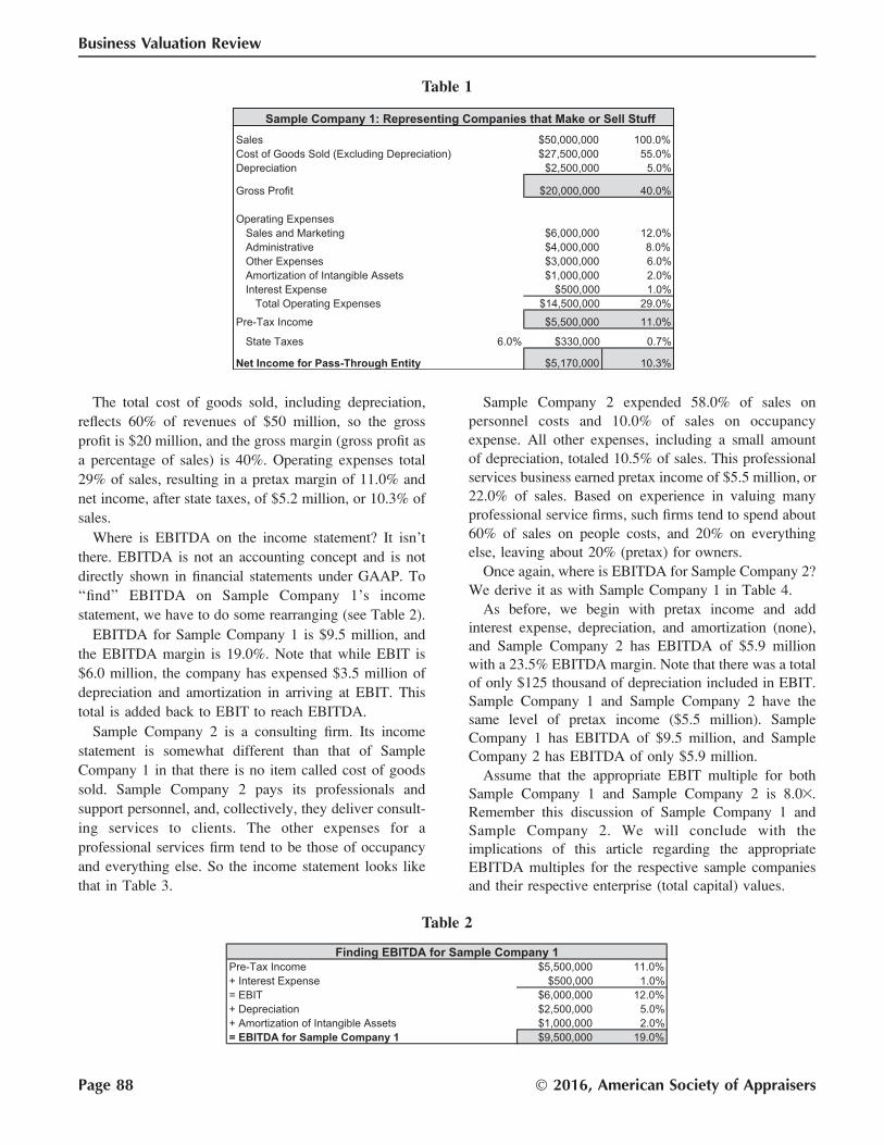
The total cost of goods sold, including depreciation,

reflects 60% of revenues of $50 million, so the gross

profit is $20 million, and the gross margin (gross profit as

a percentage of sales) is 40%. Operating expenses total

29% of sales, resulting in a pretax margin of 11.0% and

net income, after state taxes, of $5.2 million, or 10.3% of

sales.

Where is EBITDA on the income statement? It isn’t

there. EBITDA is not an accounting concept and is not

directly shown in financial statements under GAAP. To

‘‘find’’ EBITDA on Sample Company 1’s income

statement, we have to do some rearranging (see Table 2).

EBITDA for Sample Company 1 is $9.5 million, and

the EBITDA margin is 19.0%. Note that while EBIT is

$6.0 million, the company has expensed $3.5 million of

depreciation and amortization in arriving at EBIT. This

total is added back to EBIT to reach EBITDA.

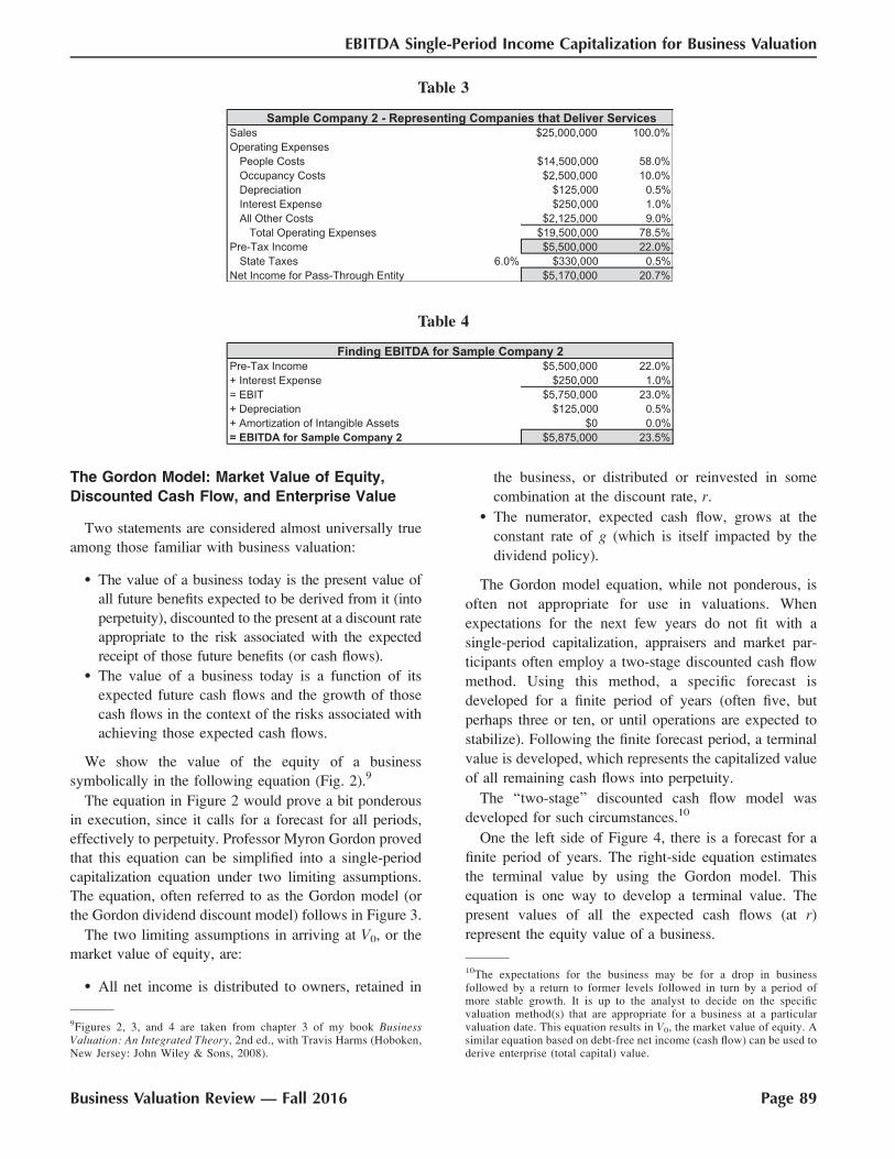
Sample Company 2 is a consulting firm. Its income

statement is somewhat different than that of Sample

Company 1 in that there is no item called cost of goods

sold. Sample Company 2 pays its professionals and

support personnel, and, collectively, they deliver consult-

ing services to clients. The other expenses for a

professional services firm tend to be those of occupancy

and everything else. So the income statement looks like

that in Table 3.

Sample Company 2 expended 58.0% of sales on

personnel costs and 10.0% of sales on occupancy

expense. All other expenses, including a small amount

of depreciation, totaled 10.5% of sales. This professional

services business earned pretax income of $5.5 million, or

22.0% of sales. Based on experience in valuing many

professional service firms, such firms tend to spend about

60% of sales on people costs, and 20% on everything

else, leaving about 20% (pretax) for owners.

Once again, where is EBITDA for Sample Company 2?

We derive it as with Sample Company 1 in Table 4.

As before, we begin with pretax income and add

interest expense, depreciation, and amortization (none),

and Sample Company 2 has EBITDA of $5.9 million

with a 23.5% EBITDA margin. Note that there was a total

of only $125 thousand of depreciation included in EBIT.

Sample Company 1 and Sample Company 2 have the

same level of pretax income ($5.5 million). Sample

Company 1 has EBITDA of $9.5 million, and Sample

Company 2 has EBITDA of only $5.9 million.

Assume that the appropriate EBIT multiple for both

Sample Company 1 and Sample Company 2 is 8.03.

Remember this discussion of Sample Company 1 and

Sample Company 2. We will conclude with the

implications of this article regarding the appropriate

EBITDA multiples for the respective sample companies

and their respective enterprise (total capital) values.

Table 1

Table 2



The Gordon Model: Market Value of Equity,

Discounted Cash Flow, and Enterprise Value

Two statements are considered almost universally true

among those familiar with business valuation:

� The value of a business today is the present value of

all future benefits expected to be derived from it (into

perpetuity), discounted to the present at a discount rate

appropriate to the risk associated with the expected

receipt of those future benefits (or cash flows).� The value of a business today is a function of its

expected future cash flows and the growth of those

cash flows in the context of the risks associated with

achieving those expected cash flows.

We show the value of the equity of a business

symbolically in the following equation (Fig. 2).9

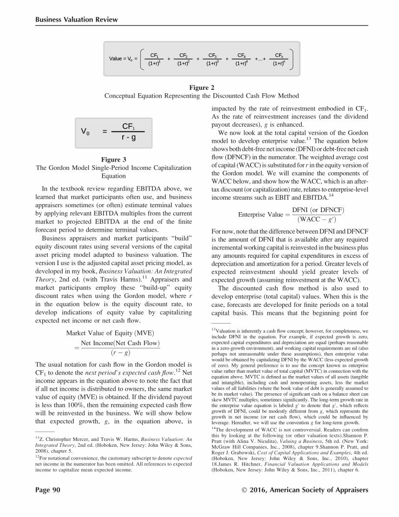
The equation in Figure 2 would prove a bit ponderous

in execution, since it calls for a forecast for all periods,

effectively to perpetuity. Professor Myron Gordon proved

that this equation can be simplified into a single-period

capitalization equation under two limiting assumptions.

The equation, often referred to as the Gordon model (or

the Gordon dividend discount model) follows in Figure 3.

The two limiting assumptions in arriving at V0, or the

market value of equity, are:

� All net income is distributed to owners, retained in

the business, or distributed or reinvested in some

combination at the discount rate, r.

� The numerator, expected cash flow, grows at the

constant rate of g (which is itself impacted by the

dividend policy).

The Gordon model equation, while not ponderous, is

often not appropriate for use in valuations. When

expectations for the next few years do not fit with a

single-period capitalization, appraisers and market par-

ticipants often employ a two-stage discounted cash flow

method. Using this method, a specific forecast is

developed for a finite period of years (often five, but

perhaps three or ten, or until operations are expected to

stabilize). Following the finite forecast period, a terminal

value is developed, which represents the capitalized value

of all remaining cash flows into perpetuity.

The ‘‘two-stage’’ discounted cash flow model was

developed for such circumstances.10

One the left side of Figure 4, there is a forecast for a

finite period of years. The right-side equation estimates

the terminal value by using the Gordon model. This

equation is one way to develop a terminal value. The

present values of all the expected cash flows (at r)

represent the equity value of a business.

Table 3

Table 4

9Figures 2, 3, and 4 are taken from chapter 3 of my book BusinessValuation: An Integrated Theory, 2nd ed., with Travis Harms (Hoboken,New Jersey: John Wiley & Sons, 2008).

10The expectations for the business may be for a drop in businessfollowed by a return to former levels followed in turn by a period ofmore stable growth. It is up to the analyst to decide on the specificvaluation method(s) that are appropriate for a business at a particularvaluation date. This equation results in V0, the market value of equity. Asimilar equation based on debt-free net income (cash flow) can be used toderive enterprise (total capital) value.



In the textbook review regarding EBITDA above, we

learned that market participants often use, and business

appraisers sometimes (or often) estimate terminal values

by applying relevant EBITDA multiples from the current

market to projected EBITDA at the end of the finite

forecast period to determine terminal values.

Business appraisers and market participants ‘‘build’’equity discount rates using several versions of the capital

asset pricing model adapted to business valuation. The

version I use is the adjusted capital asset pricing model, as

developed in my book, Business Valuation: An IntegratedTheory, 2nd ed. (with Travis Harms).11 Appraisers and

market participants employ these ‘‘build-up’’ equity

discount rates when using the Gordon model, where rin the equation below is the equity discount rate, to

develop indications of equity value by capitalizing

expected net income or net cash flow.

Market Value of Equity ðMVEÞ

¼ Net IncomeðNet Cash FlowÞðr � gÞ

The usual notation for cash flow in the Gordon model is

CF1 to denote the next period’s expected cash flow.12 Net

income appears in the equation above to note the fact that

if all net income is distributed to owners, the same market

value of equity (MVE) is obtained. If the dividend payout

is less than 100%, then the remaining expected cash flow

will be reinvested in the business. We will show below

that expected growth, g, in the equation above, is

impacted by the rate of reinvestment embodied in CF1.As the rate of reinvestment increases (and the dividendpayout decreases), g is enhanced.

We now look at the total capital version of the Gordon

model to develop enterprise value.13 The equation below

shows both debt-free net income (DFNI) or debt-free net cash

flow (DFNCF) in the numerator. The weighted average cost

of capital (WACC) is substituted for r in the equity version of

the Gordon model. We will examine the components of

WACC below, and show how the WACC, which is an after-

tax discount (or capitalization) rate, relates to enterprise-level

income streams such as EBIT and EBITDA.14

Enterprise Value ¼ DFNI ðor DFNCFÞðWACC� g0Þ

For now, note that the difference between DFNI and DFNCF

is the amount of DFNI that is available after any required

incremental working capital is reinvested in the business plus

any amounts required for capital expenditures in excess of

depreciation and amortization for a period. Greater levels of

expected reinvestment should yield greater levels of

expected growth (assuming reinvestment at the WACC).

The discounted cash flow method is also used to

develop enterprise (total capital) values. When this is the

case, forecasts are developed for finite periods on a total

capital basis. This means that the beginning point for

Figure 2Conceptual Equation Representing the Discounted Cash Flow Method

Figure 3The Gordon Model Single-Period Income Capitalization

Equation

11Z. Christopher Mercer, and Travis W. Harms, Business Valuation: AnIntegrated Theory, 2nd ed. (Hoboken, New Jersey: John Wiley & Sons,2008), chapter 5.12For notational convenience, the customary subscript to denote expectednet income in the numerator has been omitted. All references to expectedincome to capitalize mean expected income.

13Valuation is inherently a cash flow concept; however, for completeness, weinclude DFNI in the equation. For example, if expected growth is zero,expected capital expenditures and depreciation are equal (perhaps reasonablein a zero-growth environment), and working capital requirements are nil (alsoperhaps not unreasonable under these assumptions), then enterprise valuewould be obtained by capitalizing DFNI by the WACC (less expected growthof zero). My general preference is to use the concept known as enterprisevalue rather than market value of total capital (MVTC) in connection with theequation above. MVTC is defined as the market values of all assets (tangibleand intangible), including cash and nonoperating assets, less the marketvalues of all liabilities (where the book value of debt is generally assumed tobe its market value). The presence of significant cash on a balance sheet canskew MVTC multiples, sometimes significantly. The long-term growth rate inthe enterprise value equation is labeled g0 to denote that g0, which reflectsgrowth of DFNI, could be modestly different from g, which represents thegrowth in net income (or net cash flow), which could be influenced byleverage. Hereafter, we will use the convention g for long-term growth.14The development of WACC is not controversial. Readers can confirmthis by looking at the following (or other valuation texts).Shannon P.Pratt (with Alina V. Niculita), Valuing a Business, 5th ed. (New York:McGraw Hill Companies, Inc., 2008), chapter 9.Shannon P. Pratt, andRoger J. Grabowski, Cost of Capital Applications and Examples, 4th ed.(Hoboken, New Jersey: John Wiley & Sons, Inc., 2010), chapter18.James R. Hitchner, Financial Valuation Applications and Models(Hoboken, New Jersey: John Wiley & Sons, Inc., 2011), chapter 6.



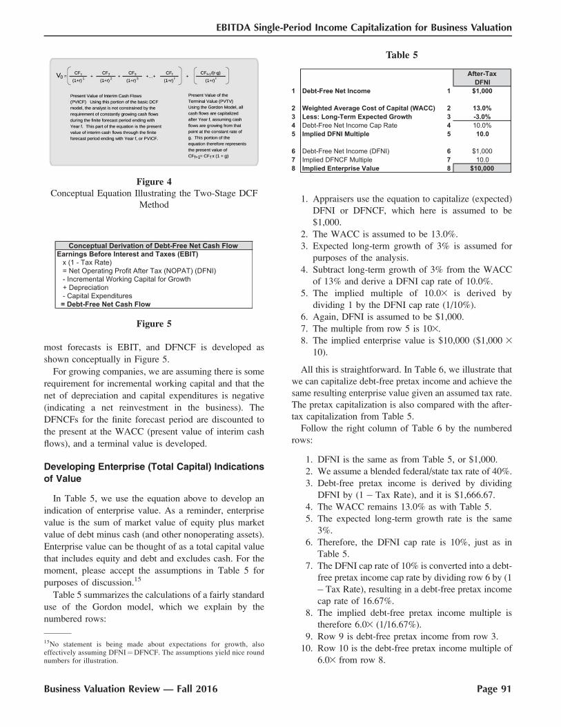
most forecasts is EBIT, and DFNCF is developed as

shown conceptually in Figure 5.

For growing companies, we are assuming there is some

requirement for incremental working capital and that the

net of depreciation and capital expenditures is negative

(indicating a net reinvestment in the business). The

DFNCFs for the finite forecast period are discounted to

the present at the WACC (present value of interim cash

flows), and a terminal value is developed.

Developing Enterprise (Total Capital) Indications

of Value

In Table 5, we use the equation above to develop an

indication of enterprise value. As a reminder, enterprise

value is the sum of market value of equity plus market

value of debt minus cash (and other nonoperating assets).

Enterprise value can be thought of as a total capital value

that includes equity and debt and excludes cash. For the

moment, please accept the assumptions in Table 5 for

purposes of discussion.15

Table 5 summarizes the calculations of a fairly standard

use of the Gordon model, which we explain by the

numbered rows:

1. Appraisers use the equation to capitalize (expected)

DFNI or DFNCF, which here is assumed to be

$1,000.

2. The WACC is assumed to be 13.0%.

3. Expected long-term growth of 3% is assumed for

purposes of the analysis.

4. Subtract long-term growth of 3% from the WACC

of 13% and derive a DFNI cap rate of 10.0%.

5. The implied multiple of 10.03 is derived by

dividing 1 by the DFNI cap rate (1/10%).

6. Again, DFNI is assumed to be $1,000.

7. The multiple from row 5 is 103.

8. The implied enterprise value is $10,000 ($1,000 3

10).

All this is straightforward. In Table 6, we illustrate that

we can capitalize debt-free pretax income and achieve the

same resulting enterprise value given an assumed tax rate.

The pretax capitalization is also compared with the after-

tax capitalization from Table 5.

Follow the right column of Table 6 by the numbered

rows:

1. DFNI is the same as from Table 5, or $1,000.

2. We assume a blended federal/state tax rate of 40%.

3. Debt-free pretax income is derived by dividing

DFNI by (1� Tax Rate), and it is $1,666.67.

4. The WACC remains 13.0% as with Table 5.

5. The expected long-term growth rate is the same

3%.

6. Therefore, the DFNI cap rate is 10%, just as in

Table 5.

7. The DFNI cap rate of 10% is converted into a debt-

free pretax income cap rate by dividing row 6 by (1

�Tax Rate), resulting in a debt-free pretax income

cap rate of 16.67%.

8. The implied debt-free pretax income multiple is

therefore 6.03 (1/16.67%).

9. Row 9 is debt-free pretax income from row 3.

10. Row 10 is the debt-free pretax income multiple of

6.03 from row 8.

Figure 4Conceptual Equation Illustrating the Two-Stage DCF

Method

Figure 5

Table 5

15No statement is being made about expectations for growth, alsoeffectively assuming DFNI¼DFNCF. The assumptions yield nice roundnumbers for illustration.



11. Row 11 is the product of rows 9 and 10, which

yields an implied enterprise value of $10,000,

which is identical to the enterprise value derived

from capitalizing DFNI.

This ‘‘proof’’ may seem trivial, but it is important for

the remainder of the article.

Note that on line 3 of Table 6 showing debt free pre-tax

income, we see the ‘‘insight’’ that debt-free pretax income

equals EBIT. This is true because pretax income plus interest

expense is earnings before interest and taxes, or EBIT.

A Single-Period Income Capitalization Techniqueto Capitalize EBITDA

With this background, we can now, using the totalcapital version of the Gordon model, build capitalization

rates and multiples for EBIT and EBITDA. A range of

equity discount rates from 15% to 20% is used in Table 7.

The components of this range include the approximate

market yield on twenty-year Treasury bonds at the time of

writing (about 2.5%), an equity risk premium of about

5.5%, a base size premium of about 6%, and additional,

specific risk factors ranging from about 1% to 6%.16

Similar assumptions are made every time appraisers

use the adjusted capital asset pricing model (CAPM) to

develop equity discount rates. The remaining assumptions

Table 6Comparison of Capitalization of Debt-Free Net Income and Debt-Free Pre-Tax Income

Table 7Developing a Range of Implied EBITDA Multiples Under a Reasonable Range of Assumptions

16For simplicity, assume that a beta of 1.03 is appropriate for the rangeof companies being considered. Further analysis can be performed toexamine the impact of beta on this analysis. On balance, we are assumingthat the companies considered range in size from perhaps $5 million invalue to $100 million or more for our purposes here.



are discussed in Table 7. I hope that no reader is offended

by the general range of assumptions, which are fairly

typical in the valuation of a broad range of private

companies.

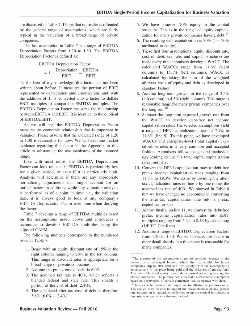
The last assumption in Table 7 is a range of EBITDA

Depreciation Factors from 1.20 to 1.30. The EBITDA

Depreciation Factor is defined as:

EBITDA Depreciation Factor

¼ 1þ Depreciation

EBIT¼ EBITDA

EBIT

To the best of my knowledge, this factor has not been

written about before. It measures the portion of EBIT

represented by depreciation (and amortization) and, with

the addition of 1, is converted into a factor to deflate

EBIT multiples to comparable EBITDA multiples. The

EBITDA Depreciation Factor measures the relationship

between EBITDA and EBIT. It is identical to the quotient

of EBITDA/EBIT.

As we will see, the EBITDA Depreciation Factor

measures an economic relationship that is important in

valuation. Please assume that the indicated range of 1.20

to 1.30 is reasonable for now. We will examine market

evidence regarding this factor in the Appendix to this

article to substantiate the reasonableness of the assumed

range.

Like with most ratios, the EBITDA Depreciation

Factor can look unusual if EBITDA is particularly low

for a given period, or even if it is particularly high.

Analysis will determine if there are any appropriate

normalizing adjustments that might account for an

outlier factor. In addition, while any valuation analysis

is performed as of a point in time, i.e., the valuation

date, it is always good to look at any company’s

EBITDA Depreciation Factor over time when deriving

the factor.

Table 7 develops a range of EBITDA multiples based

on the assumptions noted above and introduces a

technique to develop EBITDA multiples using the

adjusted CAPM.

The following numbers correspond to the numbered

rows in Table 7.

1. Begin with an equity discount rate of 15% in the

right column ranging to 20% in the left column.

This range of discount rates is appropriate for a

broad range of private companies.

2. Assume the pretax cost of debt is 6.0%.

3. The assumed tax rate is 40%, which reflects a

blended federal and state rate. This shields a

portion of the cost of debt (2.4%).

4. The calculated after-tax cost of debt is therefore

3.6% (6.0% � 2.4%).

5. We have assumed 70% equity in the capital

structure. This is in the range of equity capitali-

zation for many private companies having debt.17

6. The resulting debt capitalization is 30% (1� 70%

attributed to equity).

7. These first four assumptions (equity discount rate,

cost of debt, tax rate, and capital structure) are

made every time appraisers develop a WACC. The

calculated WACCs range from 11.6% (right

column) to 15.1% (left column). WACC is

calculated by taking the sum of the weighted

after-tax costs of equity and debt as developed in

standard fashion.

8. Assume long-term growth in the range of 3.5%

(left column) to 4.5% (right column). This range is

reasonable range for many private companies over

the long run.18

9. Subtract the long-term expected growth rate from

the WACC to develop debt-free net income

capitalization rates. The selected assumptions yield

a range of DFNI capitalization rates of 7.1% to

11.6% (line 9). To this point, we have developed

WACCs and enterprise-level (total capital) capi-

talization rates in a very common and accepted

fashion. Appraisers follow the general methodol-

ogy leading to line 9’s total capital capitalization

rates routinely.

10. Convert the DFNI capitalization rates to debt-free

pretax income capitalization rates ranging from

11.8% to 19.3%. We do so by dividing the after-

tax capitalization rates on line 9 by one minus the

assumed tax rate of 40%. We showed in Table 6

that we have changed no economics in converting

the after-tax capitalization rate into a pretax

capitalization rate.

11. Almost finally, on line 11, we convert the debt-free

pretax income capitalization rates into EBIT

multiples ranging from 5.23 to 8.53 by calculating

(1/EBIT Cap Rate).

12. Assume a range of EBITDA Depreciation Factors

from 1.20 to 1.30. We will discuss this factor in

more detail shortly, but this range is reasonable for

many companies.

17The purpose of this assumption is not to consider leverage in thecontext of a leveraged buyout, where the mix could, for largercompanies, flip to 70% debt and 30% equity, with an accompanyingenhancement in the price being paid and the riskiness of transactions.This mix of debt and equity is well above normal operating leverage forprivate companies. The purpose here is to make a reasonable assumptionbased on observation of private companies that do operate with debt.18These expected growth rate ranges are for illustrative purposes only.The analyst must be able to support the reasonableness of any growthrate assumption in valuations performed using the method introduced inthis article or any other valuation method.



13. Finally, we convert the range of EBIT multiples to

a range of EBITDA multiples by dividing the

assumed EBITDA Depreciation Factors into the

EBIT multiples developed on line 11. The

calculated range of EBITDA multiples is 4.03 to

7.13.

We have developed a range of EBITDA multiples in

Table 7. However, this technique could as well be

employed to develop a single multiple for a single-period

capitalization of EBITDA.

Until line 9, the technique is identical to that of

developing traditional WACCs and debt-free net income

(net cash flow) capitalization rates. While not shown in

Table 7, the implied debt-free net income (net cash flow)

multiples for capitalization rates of 11.6% to 7.1% (line 9)

range from 8.63 to 14.13. However, most appraisers and

market participants have no frame of reference to assess

the reasonableness of debt-free net cash flow multiples,

which are not typical market multiples considered by

market participants.

As noted above, the only additional assumption needed

to derive EBTIDA multiples is that of the EBITDA

Depreciation Factor. This factor is discussed at more length

in the remainder of this article and in its Appendix.

Analysts can examine the relationship between EBIT and

EBITDA (i.e., the EBITDA Depreciation Factor) for any

company or group of companies. They can perform similar

analyses for peer groups of private companies where such

information is available, and they can look at the

relationship for companies in guideline public company

groups. They can also examine the overall analyses of the

EBITDA Depreciation Factor for private companies and

the Standard and Poor’s (S&P) 500 (nonfinancial)

companies found in the Appendix. The information

provided will show that the range of assumptions on line

12 above is reasonable for discussion purposes.

The range of single-period EBITDA multiples devel-

oped in Table 7 is 4.03 to 7.13. Business appraisers and

market participants are familiar with EBITDA multiples.

They are calculated for every guideline transaction for

which data are available. Multiples of EBITDA are also

calculated for groups of guideline public companies by

investment bankers, stock analysts, market participants,

and business appraisers. From a practical standpoint, the

so-called rule of thumb range of 43 to 63 EBITDA, plus

or minus, that market participants and business owners

throw around, often carelessly, is confirmed by this

analysis. We do begin to see that there is an understand-

able valuation rationale for the rule of thumb ranges.

EBITDA multiples developed as in Table 7 can be used

by appraisers and market participants for two primary

purposes:

� Develop single-period income capitalizations of

EBITDA when the circumstances warrant using the

technique.� Develop the terminal value indication when using the

two-stage discounted cash flow method. The derived

EBITDA multiples facilitate comparison with EBIT-

DA multiples in the current market environment at

the time of any valuation. This method ‘‘solves’’ any

issue of ‘‘mixing’’ a market method with an income

method in using the discounted cash flow method.19

In the remainder of the article, we examine the

relationships among expected growth in cash flow, risk,

and capital intensity (as measured by the EBITDA

Depreciation Factor). The analysis is, in my view,

instructive for analysts and market participants.

Risk, Expected Growth, Capital Intensity, andEBITDA Multiples

In 1989, I wrote an article for Business ValuationReview addressing what I then called (and still do) the

adjusted CAPM.20 The article discussed how to build up

equity discount rates and to develop capitalization rates

applicable for net income (or net cash flow).

The 1989 article built on publications by James Schilt

and Shannon Pratt, who were among (and may still be)

the first to tackle the use of the CAPM to develop

discount rates and capitalization rates for business

valuation.21 The 1989 article was the first time, to my

knowledge, that a build-up method for developing equity

discount rates (and capitalization rates) considering long-

term growth was published. In that article, a range of

equity multiples was created based on ranges of

assumptions regarding expected risk and growth. The

calculated range of equity multiples was divided into four

quadrants, similar to what we will see for EBITDA

multiples below.

I have thought about extending the concept of discount

rates to pretax, total capital measures of income on a

19As I have said for years, when analysts use the Gordon model todevelop terminal value indications, it is good practice to calculate theimplied EBITDA multiples as a test of reasonableness and forcomparison with current market multiples.20Z. Christopher Mercer, ‘‘The Adjusted Capital Asset Pricing Model forDeveloping Capitalization Rates: An Extension of Previous ‘Build-Up’Methodologies Based Upon the Capital Asset Pricing Model,’’ BusinessValuation Review, 8, 4 (1989):147–156.21James H. Schilt, ‘‘Selection of Capitalization Rates for Valuing aClosely Held Business,’’ Business Valuation News (the predecessor tothe Business Valuation Review) (June 1982):2.Shannon P. Pratt, ValuingSmall Businesses and Professional Practices (Homewood, Illinois: Dow-Jones Irwin, 1986), chapter 11. Also Pratt’s Valuing a Business, 2nd ed.(Homewood, Illinois: Richard D. Irwin, Inc., 1989). Neither book hadyet provided a clear exposition for developing equity discount ratesusing the (Adjusted) CAPM, although they were moving in thatdirection. Pratt spoke of subtracting inflation (and not expected growth)from the discount rate to arrive at an equity cash flow capitalization rate.



number of occasions in the past. In particular, I was

interested in developing a single-period income capital-

ization model to capitalize EBITDA, because of the

universal nature of its use by business appraisers,

business owners, and market participants, including both

buyers and sellers of businesses.

The insight of the relationship between EBIT and

depreciation, which led to recognition of the EBITDA

Depreciation Factor, made this extension possible.

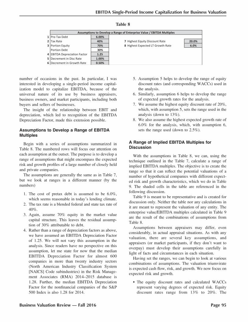
Assumptions to Develop a Range of EBITDAMultiples

Begin with a series of assumptions summarized in

Table 8. The numbered rows will focus our attention on

each assumption at the outset. The purpose is to develop a

range of assumptions that might encompass the expected

risk and growth profiles of a large number of closely held

and private companies.

The assumptions are generally the same as in Table 7,

but we look at ranges in a different manner (by the

numbers)

1. The cost of pretax debt is assumed to be 6.0%,

which seems reasonable in today’s lending climate.

2. The tax rate is a blended federal and state tax rate of

40%.

3. Again, assume 70% equity in the market value

capital structure. This leaves the residual assump-

tion of 30% attributable to debt.

4. Rather than a range of depreciation factors as above,

we have assumed an EBITDA Depreciation Factor

of 1.25. We will not vary this assumption in the

analysis. Since readers have no perspective on this

assumption, let me state for now that the median

EBITDA Depreciation Factor for almost 600

companies in more than twenty industry sectors

(North American Industry Classification System

[NAICS] Code subindustries) in the Risk Manage-

ment Associates (RMA) 2014–2015 database is

1.28. Further, the median EBITDA Depreciation

Factor for the nonfinancial companies of the S&P

500 Index is also 1.28 for 2014.

5. Assumption 5 helps to develop the range of equity

discount rates (and corresponding WACCs) used in

the analysis.

6. Similarly, assumption 6 helps to develop the range

of expected growth rates for the analysis.

7. We assume the highest equity discount rate of 20%,

which, with assumption 5, sets the range used in the

analysis (down to 13%).

8. We also assume the highest expected growth rate of

6.0% for the analysis, which, with assumption 6,

sets the range used (down to 2.5%).

A Range of Implied EBITDA Multiples forDiscussion

With the assumptions in Table 8, we can, using the

technique outlined in the Table 7, calculate a range of

implied EBITDA multiples. The objective is to create the

range so that it can reflect the potential valuations of a

number of hypothetical companies with different expect-

ed risk and growth characteristics, which we do in Table

9. The shaded cells in the table are referenced in the

following discussion.

Table 9 is meant to be representative and is created for

discussion only. Neither the table nor any calculations in

it are meant to represent the valuation of any entity. The

enterprise value/EBITDA multiples calculated in Table 9

are the result of the combinations of assumptions from

Table 8.

Assumptions between appraisers may differ, even

considerably, in actual appraisal situations. As with any

valuation, there are several key assumptions, and

appraisers (or market participants, if they don’t want to

overpay) must develop their assumptions carefully in

light of facts and circumstances in each situation.

Having set the ranges, we can begin to look at various

combinations of assumptions. The valuation triumvirate

is expected cash flow, risk, and growth. We now focus on

expected risk and growth.

� The equity discount rates and calculated WACCs

represent varying degrees of expected risk. Equity

discount rates range from 13% to 20%. The

Table 8



corresponding WACCs range from about 10% to

15%. Obviously, a company with an equity discount

rate of 13% is a different animal than one with a

corresponding equity discount rate of 20%.� The range of expected growth rates represents

varying levels of expectations for the future. The

indicated range is from 6.0% down to 2.5%. There is

a significant difference in expected growth over this

range.� Finally, each EBITDA multiple calculated in Table 9

is based on the assumptions in Table 8 and

calculations as presented in Table 7.

Focus on one combination in Table 9 to verify how the

table works. Look at the intersection of a 17% equity

discount rate and a 4.0% expected growth rate. With all

the assumptions in Table 8, this combination implies an

enterprise value to EBITDA multiple of 5.33. All of the

implied EBITDA multiples in Table 11 are calculated

similarly.

Look at the column in Table 9 with an equity discount

rate of 16%. The calculated multiples range from 4.93 to

7.63 as expected growth rises from 2.5% to 6.0%. Value,

as represented by the EBITDA multiples, is positively

correlated with expected growth. More rapid expected

growth yields higher EBITDA multiples and highervalues, all other things being equal.

Look now at the row in Table 9 with expected growth

of 4.0%. The implied EBITDA multiples range from

4.33 where the equity discount rate is 20%, up to 7.83

where the equity discount rate is 13%. Value, as

represented by the EBITDA multiple, is inversely

correlated with risk. As risk decreases, the EBITDAmultiple increases and value increases, all other thingsbeing equal.

Tradeoffs Between Expected Growth and Riskand the Impact on Value

We have, somewhat arbitrarily, divided Table 9 into

four quadrants. They are cleverly called quadrants I, II,

III, and IV. There are many implied EBITDA multiples in

Table 9. In Table 10, we show only the ranges of implied

multiples and the average multiples for each quadrant.

With fewer numbers in Table 10, we gain better insight

into how EBITDA multiples relate to varying expecta-

tions regarding expected risk and growth.

� Quadrant I—higher risk/lower growth. Companies

in quadrant I (and having all the assumptions in

Table 10

Table 9



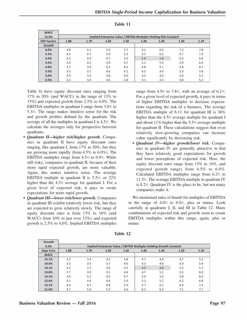
Table 8) have equity discount rates ranging from

17% to 20% (and WACCs in the range of 13% to

15%) and expected growth from 2.5% to 4.0%. The

EBITDA multiples in quadrant I range from 3.83 to

5.33. The range makes intuitive sense for the risk

and growth profiles defined by the quadrant. The

average of all the multiples in quadrant I is 4.53. We

calculate the averages only for perspective between

quadrants.� Quadrant II—higher risk/higher growth. Compa-

nies in quadrant II have equity discount rates

ranging, like quadrant I, from 17% to 20%, but they

are growing more rapidly (from 4.5% to 6.0%). The

EBITDA multiples range from 4.53 to 6.93. While

still risky, companies in quadrant II, because of their

more rapid expected growth, are more valuable.

Again, this makes intuitive sense. The average

EBITDA multiple in quadrant II is 5.53, or 22%

higher than the 4.53 average for quadrant I. For a

given level of expected risk, it pays to create

expectations for more rapid growth.� Quadrant III—lower risk/lower growth. Companies

in quadrant III exhibit relatively lower risk, but they

are expected to grow relatively slowly. The range of

equity discount rates is from 13% to 16% (and

WACCs from 10% to just over 12%), and expected

growth is 2.5% to 4.0%. Implied EBITDA multiples

range from 4.93 to 7.83, with an average of 6.13.

For a given level of expected growth, it pays in terms

of higher EBITDA multiples to decrease expecta-

tions regarding the risk of a business. The average

EBITDA multiple of 6.13 for quadrant III is 36%

higher than the 4.53 average multiple for quadrant I

and about 11% higher than the 5.53 average multiple

for quadrant II. These calculations suggest that even

relatively slow-growing companies can increase

value significantly by decreasing risk.� Quadrant IV—higher growth/lower risk. Compa-

nies in quadrant IV are generally attractive in that

they have relatively good expectations for growth

and lower perceptions of expected risk. Here, the

equity discount rates range from 13% to 16%, and

expected growth ranges from 4.5% to 6.0%.

Calculated EBITDA multiples range from 6.23 to

11.53. The average EBITDA multiple in quadrant IV

is 8.23. Quadrant IV is the place to be, but not many

companies make it.

We mentioned rules of thumb for multiples of EBITDA

in the range of 4.03 to 6.03, plus or minus. Look

carefully at quadrants I, II, and III in Table 12. Many

combinations of expected risk and growth seem to create

EBITDA multiples within this range, again, plus or

minus.

Table 12

Table 11



� Quadrant I multiples are entirely within this general

range.� Quadrant II multiples are largely within this range,

and they exceed it only with lower relative risk and

above-average growth expectations.� The average EBITDA multiple in quadrant III is 6.1,

and only companies with lower relative risk and

higher expected growth (within the quadrant) receive

multiples above this pervasive range of 4.03 to 6.03

of EBITDA multiples.� Finally, we see that to break out of the rule of thumb

range, a company needs to be in quadrant IV, where

it demonstrates both relatively lower risk and

relatively higher growth (in relationship to the other

quadrants).22

Many business owners think that the primary way to

create value is by increasing earnings. If earnings or cash

flow increase, value certainly does tend to increase, even

at the same valuation multiple.

Tables 9 and 10 suggest additional ways to work on

increasing value at any given level of earnings. EBITDA

multiples and value can also be increased by working on

the other two elements of the valuation triumvirate,

expected risk and growth. This type of analysis should

help business appraisers explain the relationships between

risk and growth and value to their business owner clients.

Look back at Table 9 at the intersections of the 16%

and 17% equity discount rate columns and the expected

growth row of 2.5%. The EBITDA multiple at a 17%

discount rate is 4.63, while the multiple at a 16%

discount rate is 4.93, or about 7% greater. Business

owners can increase value by working to reduce common

risks related to concentrations of customers, suppliers,

products, or other risks. This will not happen at once, but

over time, it is always good to be working to reduce risk,

and increasing value in the process.

Look again at Table 9 at the intersection of a 16%

equity discount rate column and the rows for expected

growth of 4.0% and 4.5%. The EBITDA multiple where

growth is 4.5% is 6.23, or 7% greater than the multiple of

5.83 where growth is 4%. Other things being equal,

increasing expected growth tends to increase multiples

and value.

Look again at the multiples we have discussed. The

multiple for a 17% equity discount rate and 4% growth

is 5.33, while the multiple for a 16% discount rate and

4.5% growth is 6.23. Consider a business owner who,

over a period of time, increased expected growth a little,

from 4% to 4.5% and lowered risk, reducing the

discount rate from 17% to 16%. The EBITDA multiple

would increase by 17%, or from 5.33 to 6.23. That

would be a worthwhile increase, and worth a bit of

effort.

The real world of market valuation is not necessarily as

precise as our examples. The lesson is nevertheless clear.

Business owners should always be working, over time, to

move to the right on Tables 9 and 10 (by reducing risk)

and up as well (by increasing growth).

Risk, Growth, and the EBITDA DepreciationFactor

In Tables 9 and 10, we examined the relationship

between EBITDA multiples and various assumptions

about expected risk and expected growth. In addition to

differences in expected risk and growth, EBITDA

multiples are also impacted by changes in relative

capital intensity. In the tables above, we assumed that

the EBITDA Depreciation Factor was fixed at 1.25. It

can obviously vary from company to company and

industry to industry, so we need to examine the impact

of relative capital intensity on EBITDA multiples, as

well.

Tables 11 and 12 provide calculations of implied

EBITDA multiples for a range of EBITDA Depreciation

Factors holding risk constant at a WACC of 13.0% while

varying expected growth (Table 11), and holding

expected growth constant at 4.5% while varying risk

(Table 12).

Table 11 illustrates the impact of changes in the

EBITDA Depreciation Factors while holding expected

growth constant (along each row). For example, a

company that could, over time, improve its EBITDA

Depreciation Factor from 1.40 to 1.30 while holding

expected growth constant at 5.0% could expect EBITDA

multiple expansion from about 5.43 to 5.83, which

would represent an improvement of about 7%.23

Table 12 holds expected growth constant at 4.5% and

varies expected risk. Look at the row where expected risk

is represented by a WACC of 14.1%. A company that,

over time, can enhance its capital efficiency from 1.40 to

1.30 (as represented by the EBITDA Depreciation Factor)

can expect an increase in its EBITDA multiple from 4.53

to 5.83, or about 7%.

22Larger companies are generally perceived to be less risky than smallercompanies. To the extent that very large companies are being valued,equity discount rates may be less than the 13% lower bound for equitydiscount rates in Tables 9 and 10. For larger companies, depending ontheir growth expectations and capital intensity, there would be a biasupward in EBITDA multiples relative to the ranges noted here.

23‘‘Improving’’ an EBITDA Depreciation Factor might result fromenhanced productivity related to plant and equipment (or software) thatdeliver the same level of EBITDA with relatively fewer depreciableassets. Note that for companies growing above an inflationary rate, therewill be some net investment of net cash flow back into the business.Appraisers need to be aware of the expected impact of growth on cashflow available for taxes and distribution. See Figure 5.



Analysis of the EBITDA Depreciation Factor can

enable the business appraiser to focus on expected risk,

growth, and relative capital intensity in developing

EBITDA multiples.

Reprise for Sample Company 1 and SampleCompany 2

Sample Company 1 has twice the level of sales as

Sample Company 2 ($50 million versus $25 million).

Sample Company 1 has EBITDA of $9.5 million (19.0%

margin), or 62% more than Sample Company 2 ($5.875

million with a 23.5% margin). Both are successful

companies. The question becomes, which is worth more?

With EBIT of $6.0 million and depreciation and

amortization expense of $3.5 million, Sample Company

1’s EBITDA Depreciation Factor is 1.58 (1þ $3.5/$6.0).

With EBIT of $5.75 million and depreciation of $125

thousand, Sample Company 2’s EBITDA Depreciation

Factor is 1.02 (1 þ $0.125/$5.875).

Recall that relevant EBIT multiple for both companies

is assumed to be 8.03. We calculate EBITDA multiples

below.

� Sample Company 1: 8.0/1.58 ¼ 5.13 EBITDA

multiple.� Sample Company 2: 8.0/1.02 ¼ 7.83 EBITDA

multiple.

Sample Company 2 has an implied EBITDA multiple

of 7.83, or more than 50% greater than the 5.13 EBITDA

multiple for Sample Company 1. Sample Company 2 is

clearly worth relatively more per dollar of EBITDA than

Sample Company 1.

The bottom line is that, relative to Sample Company 1,

Sample Company 2 delivers more dollars of EBIT from a

given dollar of sales. The result is that the markets (and

appraisers) would generally deliver a higher multiple of

EBITDA for companies like Sample Company 2, other

things being equal.

We now calculate the enterprise values for each of the

two companies.

� Sample Company 1: $9.500 million 3 5.1¼ $48.450

million.� Sample Company 2: $5.875 million 3 7.8¼ $45.825

million.

Enterprise value for Sample Company 1 is $48.45

million, while enterprise value for Sample Company 2 is

$45.825 million, or almost as much on half the sales. We

have discussed the rule of thumb range of 43 to 63

EBITDA for many private companies. The entire

discussion above shows why that rule of thumb range

exists. However, the discussion also shows that not every

company will fit into that rule of thumb range. Our

sample company analysis makes this clear. There is no

substitute for good valuation analysis that appropriately

considers the risks, expected growth, and expected capital

intensity (which impacts net cash flow) of every subject

company.

Conclusion

We began this article with a discussion addressing the

observation that EBITDA is the lowest common

denominator measure of gross cash flow with which to

compare private companies. EBITDA is the starting point

for analyzing cash flow for owners.

We then introduced the EBITDA Depreciation Factor,

which examines the relationship between DA, or

depreciation and amortization, and EBIT. The EBITDA

Depreciation Factor converts EBIT multiples to corre-

sponding multiples of EBITDA. Market evidence regard-

ing the EBITDA Depreciation Factor is provided in the

Appendix to this article.

We introduced a technique to develop implied

EBITDA multiples. Then we discussed the implications

of varying assumptions regarding expected risk, growth,

and capital intensity. Finally, we ‘‘valued’’ Sample

Company 1 and Sample Company 2 to illustrate the

impact of the EBITDA Depreciation Factor on relative

value and enterprise value.

To my knowledge, the technique we introduced for

developing capitalization rates and multiples to capitalize

EBITDA has not been published previously. This

technique requires the development of all of the

assumptions necessary to develop the WACC for a

business and requires only one additional assumption,

that of the EBITDA Depreciation Factor.

Appendix A: Market Evidence for the EBITDA

Depreciation Factor

Table 13 illustrates the generic EBITDA multiples

related to varying EBITDA Depreciation Factors. It

shows the following:

� Depreciation as a percentage of EBIT is shown

ranging from 5% to 50% on the top row for purposes

of illustration.� EBITDA Depreciation Factors are then calculated,

i.e., [1 þ (Depreciation/EBIT)], and these factors

range from 1.05 to 1.50 (second row below).� In the third row of the table, implied EBITDA

multiples are calculated based on an assumed EBIT

multiple of 8.03. We will use this as a reference

point, but know that not all businesses sell for 83

EBIT.



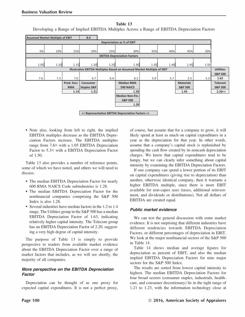
� Note also, looking from left to right, the implied

EBITDA multiples decrease as the EBITDA Depre-

ciation Factors increase. The EBITDA multiples

range from 7.63 with a 1.05 EBITDA Depreciation

Factor to 5.33 with a EBITDA Depreciation Factor

of 1.50.

Table 13 also provides a number of reference points,

some of which we have noted, and others we will need to

discuss.

� The median EBITDA Depreciation Factor for nearly

600 RMA NAICS Code subindustries is 1.28.� The median EBITDA Depreciation Factor for the

nonfinancial companies comprising the S&P 500

Index is also 1.28.� Several industries have median factors in the 1.2 to 1.4

range. The Utilities group in the S&P 500 has a median

EBITDA Depreciation Factor of 1.63, indicating

relatively higher capital intensity. The Telecom group

has an EBITDA Depreciation Factor of 2.20, suggest-

ing a very high degree of capital intensity.

The purpose of Table 13 is simply to provide

perspective to readers from available market evidence

about the EBITDA Depreciation Factor over a range of

market factors that includes, as we will see shortly, the

majority of all companies.

More perspective on the EBITDA DepreciationFactor

Depreciation can be thought of as one proxy for

expected capital expenditures. It is not a perfect proxy,

of course, but assume that for a company to grow, it will

likely spend at least as much on capital expenditures in a

year as the depreciation for that year. In other words,

assume that a company’s capital stock is replenished by

spending the cash flow created by its noncash depreciation

charges. We know that capital expenditures tend to be

lumpy, but we can clearly infer something about capital

intensity by examining the EBITDA Depreciation Factors.

If one company can spend a lower portion of its EBIT

on capital expenditures (giving rise to depreciation) than

another, otherwise identical company, then it warrants a

higher EBITDA multiple, since there is more EBIT

available for non-capex uses (taxes, additional reinvest-

ment, and dividends or distributions). Not all dollars of

EBITDA are created equal.

Public market evidence

We can test the general discussion with some market

evidence. It is not surprising that different industries have

different tendencies towards EBITDA Depreciation

Factors, or different percentages of depreciation in EBIT.

We look at the major nonfinancial sectors of the S&P 500

in Table 14.

Table 14 shows median and average figures for

depreciation as percent of EBIT, and also the median

implied EBITDA Depreciation Factors for nine major

sectors for the S&P 500 Index.

The results are sorted from lowest capital intensity to

highest. The median EBITDA Depreciation Factors for

four broad sectors (consumer staples, industrials, health-

care, and consumer discretionary) lie in the tight range of

1.21 to 1.23, with the information technology close at

Table 13Developing a Range of Implied EBITDA Multiples Across a Range of EBITDA Depreciation Factors



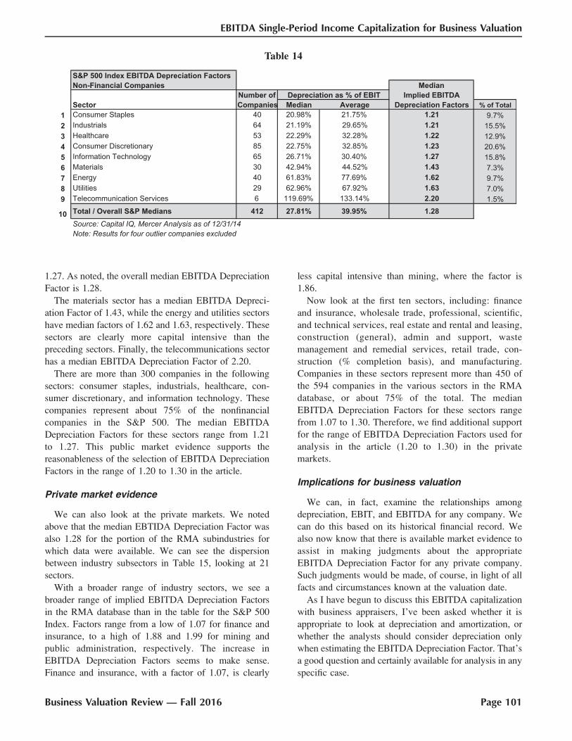
1.27. As noted, the overall median EBITDA Depreciation

Factor is 1.28.

The materials sector has a median EBITDA Depreci-

ation Factor of 1.43, while the energy and utilities sectors

have median factors of 1.62 and 1.63, respectively. These

sectors are clearly more capital intensive than the

preceding sectors. Finally, the telecommunications sector

has a median EBITDA Depreciation Factor of 2.20.

There are more than 300 companies in the following

sectors: consumer staples, industrials, healthcare, con-

sumer discretionary, and information technology. These

companies represent about 75% of the nonfinancial

companies in the S&P 500. The median EBITDA

Depreciation Factors for these sectors range from 1.21

to 1.27. This public market evidence supports the

reasonableness of the selection of EBITDA Depreciation

Factors in the range of 1.20 to 1.30 in the article.

Private market evidence

We can also look at the private markets. We noted

above that the median EBTIDA Depreciation Factor was

also 1.28 for the portion of the RMA subindustries for

which data were available. We can see the dispersion

between industry subsectors in Table 15, looking at 21

sectors.

With a broader range of industry sectors, we see a

broader range of implied EBITDA Depreciation Factors

in the RMA database than in the table for the S&P 500

Index. Factors range from a low of 1.07 for finance and

insurance, to a high of 1.88 and 1.99 for mining and

public administration, respectively. The increase in

EBITDA Depreciation Factors seems to make sense.

Finance and insurance, with a factor of 1.07, is clearly

less capital intensive than mining, where the factor is

1.86.

Now look at the first ten sectors, including: finance

and insurance, wholesale trade, professional, scientific,

and technical services, real estate and rental and leasing,

construction (general), admin and support, waste

management and remedial services, retail trade, con-

struction (% completion basis), and manufacturing.

Companies in these sectors represent more than 450 of

the 594 companies in the various sectors in the RMA

database, or about 75% of the total. The median

EBITDA Depreciation Factors for these sectors range

from 1.07 to 1.30. Therefore, we find additional support

for the range of EBITDA Depreciation Factors used for

analysis in the article (1.20 to 1.30) in the private

markets.

Implications for business valuation

We can, in fact, examine the relationships among

depreciation, EBIT, and EBITDA for any company. We

can do this based on its historical financial record. We

also now know that there is available market evidence to

assist in making judgments about the appropriate

EBITDA Depreciation Factor for any private company.

Such judgments would be made, of course, in light of all

facts and circumstances known at the valuation date.

As I have begun to discuss this EBITDA capitalization

with business appraisers, I’ve been asked whether it is

appropriate to look at depreciation and amortization, or

whether the analysts should consider depreciation only

when estimating the EBITDA Depreciation Factor. That’s

a good question and certainly available for analysis in any

specific case.

Table 14



Further, I’ve been asked what should be done if a

private company uses accelerated depreciation methods.

It might make sense to normalize depreciation in a

particular situation, just like appraisers make other

normalizing adjustments to the income statement.

The point of the questions is that analysis and judgment

are always appropriate, but this analysis is readily

performable for any company. It should be less contro-

versial than analysis and judgments made by appraisers

regarding other components of the WACC buildup.

Table 15



Documents

Quarterly Journal of the Business Valuation … VALUATION REVIEW —Published quarterly by the Business Valuation Committee of the American Society of Appraisers. TM Editor: