Embed Size (px)
Citation preview

PCBs TMDL Project – Work Order# 582-6-70860-13 –Quarterly Report No.1
Total Maximum Daily Loads for PCBs in the Houston Ship Channel
Contract No. 582-6-70860
Work Order No. 582-6-70860-13
Quarterly Report No. 1
Prepared by University of Houston
Parsons Water&Infrastructure
Principal Investigators Hanadi Rifai
Randy Palachek
PREPARED IN COOPERATION WITH THE TEXAS COMMISSION ON ENVIRONMENTAL QUALITY AND
U.S. ENVIRONMENTAL PROTECTION AGENCY
The preparation of this report was financed through grants from the U.S. Environmental Protection Agency through the Texas Commission on Environmental Quality
TCEQ Contact: Larry Koenig TMDL Team
P.O. Box 13087, MC - 203 Austin, Texas 78711-3087 [email protected]
December 2006
i

PCBs TMDL Project – Work Order# 582-6-70860-13 –Quarterly Report No.1
TABLE OF CONTENTS
TABLE OF CONTENTS ................................................................................................. ii
LIST OF TABLES ............................................................................................................ v
LIST OF FIGURES ......................................................................................................... vi
CHAPTER 1 – INTRODUCTION.................................................................................. 1
1.1 SCOPE OF THE PROJECT................................................................................ 1
1.2 DESCRIPTION OF THE REPORT ................................................................... 2
CHAPTER 2 –BACKGROUND AND PROPERTIES OF PCBs ................................ 3
2.1 BRIEF HISTORY AND BACKGROUND OF PCBs........................................ 3
2.2 PROPERTIES, SOURCES, AND FATE AND TRANSPORT OF PCBs ....... 5
2.2.1 Physical and Chemical Properties.................................................................. 5
2.3 TOXICITY AND HEALTH ASPECTS ........................................................... 11
2.3.1 Health Effects................................................................................................ 11
2.3.2 Toxic Equivalency Factors ........................................................................... 14
2.3.3 Toxicity as Related to Chemical Structure of Congeners ............................. 16
2.3.4 Maximum Contaminant Levels ..................................................................... 18
2.3.5 Regulatory Views on Toxicity ....................................................................... 19
2.4 MAJOR SOURCES OF PCBs........................................................................... 22
ii

PCBs TMDL Project – Work Order# 582-6-70860-13 –Quarterly Report No.1
2.4.1 Primary PCB Sources ................................................................................... 22
2.4.2 Recent Studies Concerning Primary Sources ............................................... 23
2.4.3 Secondary Sources ........................................................................................ 26
2.5 ENVIRONMENTAL FATE AND TRANSPORT ........................................... 27
2.5.1 Atmospheric Deposition and Air Transport.................................................. 27
2.5.2 Water Transport............................................................................................ 30
2.5.3 Sediment Transport....................................................................................... 34
2.5.3 Biological Fate.............................................................................................. 36
2.5.4 Forensics....................................................................................................... 40
CHAPTER 3 – ANALYSIS AND SAMPLING METHODS ...................................... 41
3.1 ANALYSIS METHODS........................................................................................... 41
3.2 SURFACE WATER, SEDIMENT, AND TISSUE SAMPLING.......................... 45
3.2.1 Water Sampling Methods.............................................................................. 46
3.2.2 Error Minimization in Field Sampling ......................................................... 48
CHAPTER 4 – EXISTING DATA ................................................................................ 50
4.1 – HOUSTON SHIP CHANNEL PCB DATA......................................................... 50
4.1.1 Texas Department of Health Fish Advisories ............................................... 50
4.1.2 Dioxin TMDL Project ................................................................................... 53
iii

PCBs TMDL Project – Work Order# 582-6-70860-13 –Quarterly Report No.1
4.2 OTHER RELEVANT SURFACE WATER STUDIES................................... 55
4.2.1 Shenandoah River Valley.............................................................................. 55
4.2.2 San Francisco Bay ........................................................................................ 56
4.2.3 Lake Worth, Texas ........................................................................................ 56
CHAPTER 5 – SUMMARY AND FURTHER ACTIVITIES.................................... 58
5.1 SUMMARY AND CONCLUSIONS ................................................................. 58
5.2 ACTIVITIES TO CONDUCT DURING THE NEXT QUARTER ............... 60
APPENDIX A – CONGENER PHYSICAL AND CHEMICAL PARAMETERS
APPENDIX B – PCB DATASET FROM DIOXIN TMDL PROJECT SAMPLING
REFERENCES................................................................................................................ 61
iv

PCBs TMDL Project – Work Order# 582-6-70860-13 –Quarterly Report No.1
LIST OF TABLES
Table Title Page
2.1 PCB TEFs in the TEQ-WHO98 Scheme 16
2.2 Federal PCB MCLs in Various Media and Food 19
2.3 TSCA-Mandated PCB Clean-up Levels 20
2.4 Primary Source Quantities Listed by the EPA in 1995 23
2.5 Potential PCB Coproduction Chemicals or Chemical Classes 25
3.1 NOAA Method Congener Lists 43
4.1 PCB Results From 2001 PDH Health Assessment 51
4.2 PCB Results from 2005 DSHS Health Assessment 52
4.3 Summary of Total PCB Results from the Dioxin TMDL Project 53
4.4 Summary of Aroclor Results from the Dioxin TMDL Project 54
v

PCBs TMDL Project – Work Order# 582-6-70860-13 –Quarterly Report No.1
LIST OF FIGURES
Figure Title Page
2.1 Structure of Biphenyl 6
2.2 General Structure of a PCB 6
vi

PCBs TMDL Project – Work Order# 582-6-70860-13 –Quarterly Report No.1
CHAPTER 1 – INTRODUCTION
Polychlorinated biphenyls (PCBs) are widespread organic contaminants which are
environmentally persistent and can be harmful to human health even at low
concentrations. A major route of exposure for PCBs worldwide is through food
consumption, and this route is especially significant in seafood. The discovery of PCBs
in seafood tissue has led Texas Department of State Health Services to issue seafood
consumption advisories, and some of these advisories have been issued for the Houston
Ship Channel (HSC). Two specific advisories have been issued recently for all finfish
species based on concentrations of PCBs, organochlorine pesticides, and dioxins. ADV
20 was issued in October 2001 and includes the HSC upstream of the Lynchburg Ferry
crossing and all contiguous waters, including the San Jacinto River Tidal below the U.S.
Highway 90 bridge. ADV-28 was issued in January 2005 for Upper Galveston Bay
(UGB) and the HSC and all contiguous waters north of a line drawn from Red Bluff Point
to Five Mile Cut Marker to Houston Point. These two advisories represent a large
surface water system for which TMDLs need to be developed and implemented.
1.1 SCOPE OF THE PROJECT
The scope of the TMDL PCB project includes studies and implementations related
only to PCBs in the HSC System including Upper Galveston Bay. The work included in
the scope currently includes project administration, participation in stakeholder
involvement, and development of a detailed plan for completing the PCBs TMDL. The
latter task is the bulk of the work and includes the following according to the Work Order
task numbers:
1

PCBs TMDL Project – Work Order# 582-6-70860-13 –Quarterly Report No.1
3.1.1 Collection and analysis of levels of PCBs in environmental media and sources
relevant to the HSC-UGB area.
3.1.2 Characterize the permitted and actual loading of PCBs from specific facilities or
discharges.
3.1.3 Review current technical literature to characterize the state of the science on
PCB sources, transport, and fate, which will be used to define the temporal and
spatial trends within the project area.
3.1.4 Identify data and information gaps important to the project.
1.2 DESCRIPTION OF THE REPORT
This document comprises the first quarterly report of the TMDL PCB project and
summarizes the results of the activities undertaken by the University of Houston for
Work Order No.582-6-70860-13 during the period from September 11, 2006 to
November 30, 2006.
This report reflects the progress made towards tasks 3.1.1 and 3.1.3 of the Work
Order. Chapter 2 gives a historical summary of PCBs in production, use, distribution,
analytical chemistry, and regulation in the United States. It is taken from a variety of
historical summary sources, and it serves to a give a greater context for understanding the
views and state of PCBs in the environment today. In addition, Chapter 2 presents the
results of a detailed literature review of PCB physical/chemical properties, health effects,
sources, and fate and transport. Chapter 3 presents from the literature some of the well-
established and up and coming chemical analysis and sampling methods for PCBs.
Chapter 4 summarizes PCB environmental data and information from the HSC and from
other similar PCB TMDL studies. Finally, Chapter 5 presents a summary of the activities
conducted during the reporting period and outlines the activities to be conducted in the
next quarter.
2
PCBs TMDL Project – Work Order# 582-6-70860-13 –Quarterly Report No.1
CHAPTER 2 –BACKGROUND AND PROPERTIES OF PCBS
2.1 BRIEF HISTORY AND BACKGROUND OF PCBS
Polychlorinated Biphenyls (PCBs) are a class of organic chemicals which were
first produced on an industrial scale in 1929 by the Swan Chemical Company. This
company was later purchased by Monsanto Industrial Chemicals which became the main
U.S. producer of PCBs for nearly their entire domestic production life. (De Voogt, 1989)
In the early years of PCB production, their main use was as a dielectric fluid in
transformers, but like many industrial products in that era, the end of WWII significantly
diversified the application of these chemicals and increased their levels of production.
From the late 1940s until the early 1970s, PCBs found a wide range of applications. The
main applications were dielectric fluids, heat transfer fluids in heat exchangers, and as
heat resistant hydraulic fluids. Many other smaller miscellaneous applications for PCBs
were also developed including plasticizers, carbonless copy paper, lubricants, inks,
laminating agents, impregnating agents, paints, adhesives, waxes, additives in cements
and plasters, casting agents, dedusting agents, sealing liquids, fire retardants, immersion
oils, and pesticides. (De Voogt, 1989) This latter class of applications represents only
suspected uses of PCBs and demonstrates that beyond the mainline uses, they became so
widely utilized that records do not even exist to verify all of their applications.
The environmental history of PCBs begins in 1966 when Soren Jenson, a Swede,
discovered the presence of PCBs in fish, human hair, and museum eagle feathers. He
speculated at that time that PCBs might be found in many places all over the globe and
that they might represent human and environmental health hazards. (Shifrin, 1998) The
discovery prompted an interest in environmental distribution, persistence, and toxicology
of PCBs in what had previously been a field of research concerned only with their useful
properties and their production chemistry. The interest became an intensified effort to
understand the effects and dangers of PCBs when in 1968 a group of people consuming
3

PCBs TMDL Project – Work Order# 582-6-70860-13 –Quarterly Report No.1
rice oil contaminated with PCBs at levels of 1000 ppm in Yusho, Japan showed some
serious health effects. (Shifrin, 1998)
It was then only a short number of years for the concern with PCBs to turn into an
outright national ban on their production and investigation of how to quantify and remove
them from the environment. In 1971, Monsanto voluntarily limited its production of
PCBs due to the growing public and scientific concerns of their effects (De Voogt,
1989), and in 1976 the Toxic Substances Control Act (TSCA) was passed which called
for a ban on all production, distribution, and use of PCBs. (USEPA, 2003) Monsanto’s
compliance with TSCA resulted in a complete cessation of PCB production in mid-1977,
and PCBs have not been produced industrially in the U.S. ever since. (De Voogt, 1989)
Long-life PCB applications such as transformers were still allowed under strict
regulations for operations and disposal, but those uses will eventually be completely
phased out as the old technologies are replaced.
From the time of Jenson’s discovery and into the 1970s, the international
scientific and health community made it a priority to discover how toxic PCBs really
were and what to do about them. It was clear that they were toxic enough to be banned
from production, but the exact degree of toxicity would be something which was argued
about in the scientific literature even until today.
The technology to analyze PCB samples from the environment was not well
developed enough to characterize what specific PCBs were present and to what degree.
So in addition to a rapid development of toxicological study, the analytic chemists
performed a great deal of research from the mid-1970s to the present to quantify PCBs.
That research did not culminate into any standard method of PCB analysis until the EPA
issued Method 608 in the SW-846 manual in 1982, which was used only for PCB Aroclor
mixtures. (Shifrin, 1998) Moreover the complete list of PCB congeners* could not be
quantified using GC until Schultz et al. performed the first successful analysis in 1989.
(Shifrin, 1998) The EPA has more recently provided a measure of congener-specific
* Congener is a term in chemistry that refers to one of many variants or configurations of a common chemical structure. For PCBs, each configuration of the base compound biphenyl containing two or more chlorines is its own congener.
4

PCBs TMDL Project – Work Order# 582-6-70860-13 –Quarterly Report No.1
analysis in Method 8082. Method 8082 can be used to get Aroclors and is listed to
measure 19 of the total 209 congeners. (USEPA, 1996) A complete congener distribution
high resolution PCB analysis in standard methods 1668 and 1668A(USEPA, 1999). This
body of work brings the analysis of today’s samples to high levels of detection and
resolution though regulations themselves do not require such resolution as yet.
PCBs are generally not produced, distributed, processed, or used for any
application. They are, however, nearly ubiquitous in the environment even in polar
regions far from anywhere they were ever produced or used. Thus, recent studies have
focused on three main areas: toxicology, chemical analysis, and fate and transport.
2.2 PROPERTIES, SOURCES, AND FATE AND TRANSPORT OF PCBS
2.2.1 Physical and Chemical Properties
Physicochemical properties of PCBs have been extensively studied since they
became and environmental issue in the late 1970s as evidenced by the extensive body of
literature available. However, because their properties are difficult to measure, the
reported constants for some of the environmentally-relevant properties range within
several orders of magnitude.
2.2.1.1 Chemical Classification, Structure, and Nomenclature of PCBs
Polychlorinated Biphenyls are a member of a class of compounds called
polychlorinated aromatic hydrocarbons (PCHs). PCHs are compounds containing
multiple aromatic rings bonded together in combination with multiple chlorine atoms
which are usually bound up on one of the carbon joints on an aromatic ring. PCBs are
distinct within PCHs in that their chemical structure is based off of the biphenyl molecule
as shown in Figure 2.1.
5

PCBs TMDL Project – Work Order# 582-6-70860-13 –Quarterly Report No.1
Figure 2.1 Structure of Biphenyl
As can be seen biphenyl is simply two C6 aromatic rings joined together a by a single
covalent bond. A PCB is a biphenyl which has at least two chlorine atoms attached
somewhere on one or both of the two aromatic rings. A general PCB structure for this
arrangement is shown in Figure 2.2.
Figure 2.2 General Structure of a PCB
Each ring has two ortho, two meta, and one para position on it, and the particular number
and arrangement of chlorines in these positions gives 209 theoretical combinations each
of which is called a congener.
There are two systems of nomenclature for each of the 209 congeners. The first is
the IUPAC system of nomenclature which simply lists the positions of each chlorine on
the biphenyl, followed by the Greek prefix for the number of chlorines on the biphenyl
6

PCBs TMDL Project – Work Order# 582-6-70860-13 –Quarterly Report No.1
and finally simply the word “biphenyl”. So, for example, a biphenyl with 4 chlorines at
the 2, 3, 4’, and 6 positions would be called 2,3,4’,6-Tetrachlorobiphenyl. The second
nomenclature system was developed by Ballschmiter et al. (1980) and is simply a number
of the PCB congeners in order of increasing chlorination and increasingly higher position
numbers of that chlorination. Under their system for example, 2,3,4’,6
Tetrachlorobiphenyl is called PCB64. A full table of all congeners under their IUPAC
and Ballschmiter (BZ) nomenclature has been created by the EPA and is available at
http://www.epa.gov/toxteam/pcbid/table.htm.
PCBs were not normally produced industrially (and there are no non
anthropogenic sources of PCBs) as a single pure congener product. One of the reasons
for the congener mixture was because of the production chemistry. The reaction was
always conducted at near atmospheric pressure as a batch chlorination of biphenyl with
anhydrous chlorine gas. The result was a broad mixture of many PCB congeners which
were subsequently separated and purified into more specific fractions. Each fraction,
however, still contained several congeners. (De Voogt, 1989)
The mixtures were always marketed as technical grade liquids under various trade
names such as Aroclor in the U.S., Kanechlor in Japan, and Clophen in Germany to name
but a few. (De Voogt, 1989) The Aroclor mixtures had a number designation which
followed the Aroclor name to signify the number of carbon atoms in biphenyl and the
percentage of chlorine by mass in the mixture as a whole. Thus, Aroclor 1260 contains
12 carbon items that make up the biphenyl skeleton and 60% chlorine by mass when the
congener composition of the entire mixture was taken into account. The chlorine
percentage gave the mixture different physical properties to make each mixture more
suited for particular applications.
2.2.1.2 Water Solubility
The hydrophobic nature of PCBs means that in general water solubilities are low.
The EPA agrees with this assessment but acknowledges that though all of the PCBs have
7
PCBs TMDL Project – Work Order# 582-6-70860-13 –Quarterly Report No.1
low solubilities, the differences in solubility among the congeners can still vary within
several orders of magnitude. (USEPA, 2003)
Huang and Hong (2002) found that for coplanar PCBs, within a homolog group,
the congeners that have greater ortho substitution generally have greater water solubility.
They also found that the aqueous solubility of 12 PCB congeners increased exponentially
with temperature. Huang and Hong crafted a model to predict the solubility of all 209
PCB congeners based on the melting point and chlorine substitution pattern, but they
acknowledged that more needed to be known in the area of solubility of coplanar PCBs
specifically and PCBs in general. Shiu (2000) performed a comprehensive review of
literature PCB solubilities, which is another source of some useful values.
Solubility data from the Huang (2002)study and Mackay (1992)are given in
Appendix A.
2.2.1.3 Vapor Pressure
In general, the vapor pressures of all PCBs are low though there are order of
magnitude variations among them. (USEPA, 2003) Bidleman showed that with each
addition of chlorine, the vapor pressure decreased by around a factor of 4.5. Some
representative data was found for vapor pressures by Bidleman (1984) and Paasivirta
(1999) and is presented in Appendix A.
2.2.1.4 Henry’s Law Constant
Henry’s law constants are useful in many aspects of PCB transport in water, but
the most direct use of Henry’s law constants is in the characterization of water-air
volatilization equilibrium.
A representative set of Henry’s Law constants for some congeners is given in
Appendix A by Bamford (2000) and Fang (2006).
8

PCBs TMDL Project – Work Order# 582-6-70860-13 –Quarterly Report No.1
2.2.1.5 Octanol/Water Constants
The octanol-water partitioning coefficient (Kow) is an extremely important
constant for each PCB congener since it describes the partitioning behavior of congeners
between water, soil, and biota. Hawker and Connell (1988) presented a paper which
analyzed 13 congeners and used those results to get predicted Kow’s based on assumed
log-log relationship between Kow and GC retention time. That relation is of the form
log K OW = 1.47 logα + 5.52
where α is the GC retention time. The paper by Hawker and Connell (1988) has been
cited in at least 370 articles and is a good source for Kow values.
A summary of PCB Kow values reported in the literature is presented in Appendix A..
2.2.1.6 Organic Carbon-Normalized Partition Coefficient
The organic carbon-normalized partition coefficient is a measure of partitioning
of a compound between a soil/sediment particle and water. It is usually denoted as KOC
where the OC stands for organic carbon. The organic carbon amount in the soil/sediment
matrix is important because the KOC value is highly dependent on the level of organic
carbon as evidenced by the equations below that are given and elucidated more fully by
Hansen (1999).
The octanol-water coefficient can be measured experimentally, and there are
empirical correlations available to relate Kow to KOC. A more rigorous method, however,
to measure KOC is to measure the distribution coefficient, a non-equilibrium constant
denoted as KD. It describes the soil-water partitioning for trace amounts of PCBs and is
defined as
9

PCBs TMDL Project – Work Order# 582-6-70860-13 –Quarterly Report No.1
K = C / CD S W
where CS and CW are the concentrations of the chemical in the soil and water phases,
respectively. Once this trace partitioning constant is found experimentally, a general
relationship for KOC is
†KOC = K D / fOC
where fOC is the fraction of organic carbon in the soil/sediment matrix. Strictly speaking
the distribution coefficient is not proportional to KOC because the distribution coefficient
is not based on equilibrium (CS and CW are not at equilibrium values), and KOC is an
equilibrium value. The partition coefficient KP is truly an equilibrium constant (CS and
CW are at equilibrium values) which KD will approach with time, and it is the KP which is
technically proportional to the KOC as shown
K OC = K P / f OC
Hansen was speaking, however, in a context in which KOC’s were being measured and
evaluated in experimental situations, and it is often more practical to assume that the KD
is being measured and to use it like a KP rather than to wait what could be a prohibitive
amount of time to reach equilibrium.
Thus it is seen that the organic carbon-normalized partition coefficient can be
found two ways. One way uses empirical correlations relating KOC to the PCB water
octanol relationship, and the second way uses the PCB soil-water partitioning relationship
at low PCB concentrations with the fraction of organic carbon in the media of concern.
† In the application of KOC to soils and sediments, this relation should hold up quite well. It should be remembered, however, that the polarity of the organic matter will also play a large role in PCB partitioning. Thus, in biological media such as lipids, which are highly polar, this relationship will not be enough to fully conceptualize and model PCB transport.
10

PCBs TMDL Project – Work Order# 582-6-70860-13 –Quarterly Report No.1
Thus, for the purposes of the PCB TMDL project, the characterization of
sediment-water partitioning of PCBs would depend heavily on the understanding of the
organic carbon content and behavior of either suspended particles in the water column or
deposited sediments. In the interest of providing some quantitative values (while
acknowledging that there are many other values that could have been chosen) for KOC the
data from two studies both provided in Hansen (1999) on three kinds of soils which were
averaged together are presented in Appendix A. It should be noted that this dataset will
certainly show trending in partitioning behaviors between different congeners, but there
is no reason to assume that the soil used to get these KOC values is in anyway similar to
sediment media that might be found in the HSC.
2.3 TOXICITY AND HEALTH ASPECTS
2.3.1 Health Effects
The health effects of PCB exposure can be grouped into two categories:
occupational/accidental exposure and environmental exposure. The reason for the
categorization of exposure is that generally occupational/accidental exposure to PCBs is
resultant from some large quantity event-based (acute) exposure while environmental
exposure is more long-term and accumulative (chronic). The effects of the different
exposure types in humans can be quite different.
2.3.1.1 Occupational/Accidental Exposure
There have not been large data sets on heavy dose human exposure of PCBs other
than a few well known exposure accidents from which many conclusions have been
drawn. The two refernced incidents happened in 1968 and 1978 in Fukuoka, Japan and
Taiwan, respectively. Both exposures involved PCB contamination of rice, and the
symptoms of that exposure have since been called Yusho rice oil disease. (George, 1988)
11

PCBs TMDL Project – Work Order# 582-6-70860-13 –Quarterly Report No.1
The Agency for Toxic Substances and Disease Registry (ATSDR) characterizes
symptoms of PCB exposure in “Yusho rice oil disease”. Skins affects from the exposure
include chloracne and rashes. In addition, there is evidence of liver damage. (ATSDR,
2000)
The full range of health effects that have been observed to one degree or another
by the ATSDR include the following: liver, thyroid, dermal and ocular changes,
immunological alterations, neurodevelopmental changes, reduced birth weight,
reproductive toxicity, and cancer. (ATSDR, 2000) Many of these effects arise at
increasingly higher dosages of PCBs.
2.3.1.2 Environmental Exposure
Most of the general population will encounter PCBs through environmental
exposure in air, water, soil, and food. Yet the primary exposure pathway is through food,
especially fish. (ATSDR, 2000) PCBs can be found in nearly all world populations to
some degree due to their large-scale global transport. This ubiquity in populations occurs
in both diets that include fish and diets that do not include fish. Studies involving non-
fish eating individuals showed mean serum concentrations of PCB in the range of 0.9-1.5
ppb. (ATSDR, 2000) Thus when human PCB exposure amounts are discussed, this
background level of PCBs found in nearly all populations needs to be considered before
assessing a population as having a higher PCB health risk.
Studies involving animals which consumed large quantities of food containing
PCBs showed symptoms of immunal system changes, behavioral alterations, and
impaired reproduction. (ATSDR, 2000) It is likely that an individual who consumed
PCB-contaminated food which led to PCB bioaccumulation in adipose tissue could show
similar effects.
12

PCBs TMDL Project – Work Order# 582-6-70860-13 –Quarterly Report No.1
2.3.1.3 Carcinogenicity
The toxicological community has not been able thus to far to say with absolute
certainty that PCBs are carcinogenic. Both the Department of Health and Human
Services (DHHS) and the International Agency for Research on Cancer (IARC) list PCBs
as probably carcinogenic. These carcinogenic determinations were made based mainly
on the overwhelming amount of animal exposure data, which unequivocally show PCBs
to be carcinogenic to animals. The combination of definitive evidence in animals
combined with the suggestive evidence in humans makes PCBs as a chemical class a very
likely carcinogen. (ATSDR, 2000)
2.3.1.3 General Toxic Effect and Exposure Levels
ATSDR acknowledges that although there is a strong evidence of toxicity from
exposure to PCBs, it is difficult to link a particular health effect to a particular congener.
This difficulty results from the fact that observations of exposure are usually made on
congener mixtures. So separating out one congener’s effect from another is difficult and
the interactions between the different congeners have not yet been determined. (ATSDR,
2000)
So in the knowledge that PCBs do exhibit toxicological effects (though these
effects are not linked to particular congeners or Aroclors), the ASTDR has derived some
Minimum Risk Levels (MRLs). The intermediate-duration oral exposure (15-364) days
is 0.03 ug/kg/day, and the chronic-duration oral exposure (>364 days) is 0.02 ug/kg/day.
An inhalation MRL could not be determined due to insufficient human and animal data.
(ATSDR, 2000)
13

PCBs TMDL Project – Work Order# 582-6-70860-13 –Quarterly Report No.1
2.3.2 Toxic Equivalency Factors
PCBs are part of a larger class of toxic compounds that include polychlorinated
dibenzo-p-dioxins (PCDDs) and polychlorinated dibenzofurans (PCDFs). The
correlation between the similar toxicological properties of PCDDs and PCDFs was noted
by the Ontario Ministry of the Environment in 1983, and the Ministry at that time drafted
the first document that attempted to standardize the way that different PCDDs and
PCDFs (all generally called “dioxins”) were to be toxicologically quantified. (USEPA,
2003) The method that was developed employed the use of Toxic Equivalency Factors
(TEFs), and the concept is still used as the standard today.
The way that TEFs are used is to quantify the toxicity of any one congener
relative to a reference congener. This can be done for any PCDD, PCDF, or a “dioxin
like” PCB. The referenced compound that was originally chosen was 2,3,7,8-TCDD. It
is shown to have the highest toxicity of all dioxins and dioxin-like PCBs, and its toxicity
is also the best understood. So the TEF for 2,3,7,8-TCDD is 1.0, and every other
congener has a TEF which is some fraction of 1.0. The TEFs are essentially used as a
means to scale the concentration of each congener in the environment by its toxicological
potency. When these potencies are added together, a Toxic Equivalency Quotient (TEQ)
results
k
TEQ =∑Cn ∗TEFn n=1
The method has been altered slightly throughout its history, but in that time it has become
widely accepted by the environmental community with specific approvals from the
USEPA, NATO, WHO and others. (USEPA, 2003)
14

PCBs TMDL Project – Work Order# 582-6-70860-13 –Quarterly Report No.1
2.3.2.1 PCBs in the TEF Scheme
Of the 209 PCB congeners, only 12 show “dioxin-like” toxicity. Most PCB
congeners have some relevant level of toxicity to be considered, but the TEF scheme
focuses only on organic compounds whose toxicological properties are similar to dioxins.
In 1994, the WHO European Centre for Environmental Health and the International
Programme on Chemical Safety attempted to gather all of the toxicological literature
available on all of the PCB congeners in order to make a list of those with dioxin-like
toxicity. The criteria that were used to determine which congeners made the list were:
1. Structural similarity to PCDDs and PCDFs
2. Ability to bind to the Ah receptor in the human body
3. Dioxin-specific biochemical and toxic response
4. Persistence and accumulation in the food chain
The final list (1998 latest revision) contained only 12 of the potential 209 congeners. For
these select 12, TEFs were assigned (Table. 2.1) These 12 are PCB-77, PCB-81, PCB
105, PCB-114, PCB-118, PCB-123, PCB-126, PCB-156, PCB-157, PCB-167, PCB-169,
and PCB-189.
15

PCBs TMDL Project – Work Order# 582-6-70860-13 –Quarterly Report No.1
Table 2.1 PCB TEFs in the TEQ-WHO98 Scheme
IUPAC Number Chlorination Level TEF PCB-77 Tetra-chlorinated 0.0001 PCB-81 Tetra-chlorinated 0.0001 PCB-105 Penta-chlorinated 0.0001 PCB-114 Penta-chlorinated 0.0005 PCB-118 Penta-chlorinated 0.0001 PCB-123 Penta-chlorinated 0.0001 PCB-126 Penta-chlorinated 0.1 PCB-156 Hexa-chlorinated 0.0005 PCB-157 Hexa-chlorinated 0.0005 PCB-167 Hexa-chlorinated 0.00001 PCB-169 Hexa-chlorinated 0.01 PCB-189 Hepta-chlorinated 0.0001
Source: (USEPA, 2003)
TEFs in connection with PCBs are mentioned here because they are linked topics.
It is noted, however, that this focus of this project is towards a total PCB TMDL. Thus,
while dioxin-like toxicity is an important consideration, it will not be a focal point of this
study since all PCBs need be considered regardless of how much toxicological similarity
they have to dioxins.
2.3.3 Toxicity as Related to Chemical Structure of Congeners
It is valuable to mention a structural distinction in PCB called coplanarity or what
is seen in the literature as “coplanar PCBs”. This structural class of PCB compounds has
physical and chemical properties which often differ from the rest of PCBs, but the
greatest differences in coplanar PCBs are that these PCBs are far more toxic than non-
coplanar PCBs.
PCBs (as shown in section 2.2.1.1) can be extremely varied in chemical structure
as mainly determined by the points of chlorine substitution on the aromatic rings.
Experience and study have shown that PCBs which are chlorinated at both meta positions
and one or two para positions assume a chemical conformation of coplanarity, a situation
16

PCBs TMDL Project – Work Order# 582-6-70860-13 –Quarterly Report No.1
where both phenyl rings are in the same plane. Incidentally, these substitutions often
mean that the ortho position on the rings is either “mono-ortho” or “non-ortho”
substituted, which is another way of referring to coplanar PCBs. (Metcalfe, 1995)
Many sources have pointed that coplanar PCBs have been shown to exhibit
greater toxicity than other PCB congeners. This is reflected quantitatively by the TEF
schemes which include only particular PCBs in their structure. Similarly the EPA
presents only 12 of the 209 PCB congeners as having “dioxin-like toxicity”. The EPA
states that these PCBs are structurally similar in that they have “four or more lateral
chlorines (chlorines at the meta and para positions) and one or no chlorines at an ortho
position.” (USEPA, 2003) The scientific literature also shows that coplanar PCBs are
studied heavily as a contaminant subclass ever since congener-specific GC analysis was
made more accurate and available.
The explanation given for the greater toxicity of coplanar PCBs is a chemical
analogy. The fact that these PCBs become structurally coplanar gives them a molecular
size, configuration, and chlorination pattern fairly similar to 2,3,7,8-TCDD. (Huang,
2002) Thus for many of the reasons that 2,3,7,8-TCDD has the highest TEF in the TEF
scheme so coplanar PCBs are also more toxic over their non-coplanar cousins.
Thus, non- and mono-ortho PCBs present a higher level of toxicity among the
larger class of PCBs. The toxicity is variable depending on the species, but the toxicity is
still higher in general. (Ayris, 1997) Furthermore, in the greater picture of TEQ from all
dioxin-like compounds, coplanar PCBs can play a significant role due to the combination
of moderate toxicity and relatively higher concentration. This is so much so that even in
environments where there are also high levels of PCDDs and PCDFs, there are often
more toxic equivalents as resulted from coplanar PCBs than from PCDDs and PCDFs.
(Smith, 1990)
Tanabe (1987)found that coplanar PCBs were a smaller fraction of the total PCB
concentration in marine and terrestrial biota collected from areas around Japanese seas.
Non-coplanar PCBs were on the order of parts per million while the coplanar PCBs were
on the order of parts per billion. Yet these coplanar PCBs still are much higher than the
17

PCBs TMDL Project – Work Order# 582-6-70860-13 –Quarterly Report No.1
parts per trillion concentrations normally found in PCDD/Fs in these environments.
Thus, these PCBs present as great a risk or greater a risk than dioxins due to the higher
concentrations despite a much lower level of toxic potency.
The high levels of PCBs in portions of the Laurentian Great Lakes have been
known for quite some time, and these lakes also contain concentrations of PCDD/Fs. In
this environment, coplanar PCBs may account for over 95% of the dioxin like activity
affecting the biota of the Great Lakes. (Metcalfe, 1995) In genera,l it is seen that studies
from Japan, Sweden, Finland, and North America on species including fish, wildlife, and
humans have all shown that 90% of the toxic burden from Halogenated Aromatic
Hydrocarbons (HAHs)was from coplanar PCBs and not from other PCBs, dioxins, or
dibenzofurans. (Metcalfe, 1995)
Some studies show that in air, coplanar PCBs may not be a majority of the TEQ
in air media. Kurokawa et al. found in atmospheric samples over both summer and
winter that the contribution of coplanar PCBs to total dioxin toxicity was only 4.9%.
(Kurokawa, 1996) The significance of understanding the levels and behavior of coplanar
PCBs then can be seen in aquatic environments and merits special consideration in any
study seeking to lower the risk in PCB-contaminated waters.
2.3.4 Maximum Contaminant Levels
The Maximum Contaminant Levels (MCLs) for PCBs in various media and food
products are shown in Table 2.2. The toxicity and especially the potentially carcinogenic
activity of PCBs drive the MCLs to fairly conservative values.
18

PCBs TMDL Project – Work Order# 582-6-70860-13 –Quarterly Report No.1
Table 2.2 Federal PCB MCLs in Various Media and Food
Media Level Agency Drinking Water 0.5 ppb USEPA Lakes and Streams 0.17 ppt USEPA Infant and Junior Foods 0.2 ppm FDA Eggs 0.3 ppm FDA Milk and Dairy Products 1.5 ppm FDA Fish and Shellfish 2 ppm FDA Poultry and Red Meat 3 ppm FDA Source: (ATSDR, 2000)
On the issue of the rationale behind the drinking water standard set by the EPA, they state
that, “given present technology and resources, this is the lowest level to which water
systems can reasonably be required to remove this contaminant should it occur in
drinking water.” The Maximum Contaminant Level Goal (MCLG) for PCBs is zero.
(USEPA, 2006)
2.3.5 Regulatory Views on Toxicity
2.3.5.1 National Regulations
There are three main national regulations for PCBs:
1. The Clean Water Act of 1972 (Amended several times since)
2. The Toxic Substances Control Act (TSCA) of 1977
3. The Comprehensive Environmental Response, Compensation, and Liability Act
(CERCLA) of 1980
The Clean Water Act gives the federal government authority to assign and enforce the
MCLs that were mentioned previously. Even more relevant to this project, section
19

PCBs TMDL Project – Work Order# 582-6-70860-13 –Quarterly Report No.1
303(d) of the Clean Water Act is the statute that authorizes the TMDL program for
noncompliant water bodies.
The TSCA was the first piece of legislation that mentioned PCBs directly within its
writing. The TSCA ended the production, distribution, and importation of PCBs into this
country in 1977. There were also provisions in the act that required all transformers that
used PCBs to be sealed and eventually phased out. The EPA also established a “TSCA
spill policy” in 1987 that dictated the following cleanup levels of all PCBs spilled post
1987.
Table 2.3 TSCA-Mandated PCB Clean-up Levels
Media Access Type Enforceability Clean Soil Depth Level Soil Restricted Required N/A 25 ppm Soil Unrestricted Required 10 in 10 ppm Soil Unrestricted Required 0 in 1 ppm Soil Restricted Recommended N/A 100ug/100 cm2
Soil Unrestricted Recommended N/A 10ug/100 cm2
CERCLA (commonly referred to as Superfund) affects PCBs only as they relate to
cleanup at sites polluted prior to 1987. The cleanup levels for these sites are made on a
case-by-case basis, and the “starting points” for PCB sites are 1 ppm for residential and
10-25 ppm for industrial. (Shifrin, 1998)
An attempt was made in 1994 to consolidate all of the statutes, policies, and
guidance materials on PCBs into PCB Disposal Amendments commonly known as the
“PCB megarule”. (Shifrin, 1998) That rule was finally enacted on June 29, 1998, and its
main adjustments to TSCA involve more flexibility and clarification in the disposal and
handling of PCBs and PCB wastes. (USEPA, 1998)
20

PCBs TMDL Project – Work Order# 582-6-70860-13 –Quarterly Report No.1
2.3.5.2 State of Texas Regulations
Surface water quality is regulated in the State of Texas under Title 30 Texas
Administrative Code Chapter 307. The Texas Surface Water Quality Standards (§307.1
307.10) include human health water quality criteria for total PCBs (based on Aroclors) of
1.3 ng/L and 0.885 ng/L in freshwater and saltwater, respectively. These concentrations
are lower than the MCL for drinking water due to the fact that the highest exposure
potential of PCBs in waters is through the bioaccumulation potential and consumption of
contaminated fish (Webster et al. 1998). Additionally, fresh and saltwater criteria differ
because it is assumed that consumption rates are higher for saltwater species.
The Texas Department of Health based its health assessment of PCBs in the
Houston Ship Channel (TDH, 2001 and 2006) on a screening level of 47 ng-Aroclor/g
tissue. This screening value was derived from an EPA chronic oral reference dose (RfD)
for Aroclor 1254 of 0.00002 mg/kg/day .
There also is a state established PCB Advisory Group made up of volunteers
whose purpose is to discuss the current Texas regulation on PCB analysis. This
regulation is currently listed under Title 30 Texas Administrative Code 350.76(d), and it
specifies Aroclor-based analysis methods. The advisory seeks to provide legislative
advisory to a changeover from an Aroclor based analysis to a congener specific analysis
method. Their information may be found on the TCEQ website at
http://www.tceq.state.tx.us/remediation/trrp/pcb_group.html. More discussion on current
analysis methods is given in Section 3.1.
21
PCBs TMDL Project – Work Order# 582-6-70860-13 –Quarterly Report No.1
2.4 MAJOR SOURCES OF PCBS
As was noted in the historical section of this report, PCBs have not been produced
in the Unite States since 1977. An estimate of the amount of PCBs produced globally
between 1929 and 1979 is 1.5 million metric tons. (De Voogt, 1989) Large–scale
disposal continued for some time after the cessation of production, but at present there
are few primary sources of PCBs to the environment. Most PCBs that enter a particular
water body or biosphere are transported from another contaminated environment and are
thus secondary sources.
2.4.1 Primary PCB Sources
The EPA states that “no significant release of newly formed dioxin-like PCBs is
occurring in the United States.” While the EPA acknowledges that waste combustion can
yield small amounts of PCBs, they contend that these sources are not significant and that
all significant sources of PCBs are from past production, use, and disposal. (USEPA,
2003) The EPA’s statement is directed mostly towards the “dioxin-like” PCBs (which
are nearly synonymous with the coplanar PCBs as discussed in a previous section), but
since most of the historical primary sources released both coplanar and non-coplanar
PCBs, it is reasonable to say that there are no significant releases of any newly formed
PCBs (dioxin-like or not dioxin-like).
PCBs were once sourced to the environment by way of production, use, and disposal.
Now disposal is likely the only they enter the environment. There are four main methods
of disposal that still occur (USEPA, 2003):
• Large Amount PCB Disposal (>2 pounds): Dielectric fluids from transformers
and large capacitors, which are disposed according to regulations.
• Small Amount PCB Disposal (<2 pounds): Disposal of small capacitors, light
fixtures, and waste papers in municipal landfills.
22

PCBs TMDL Project – Work Order# 582-6-70860-13 –Quarterly Report No.1
• Leaks and spills from devices that still contain PCBs.
• Illegal PCB disposal
The EPA gives four quantified primary sources for PCBs as estimated in 1995 which are
shown in Table 2.4. All are quite small in comparison to the total annual production of
PCBs during any year between 1929 and 1977.
Table 2.4 Primary Source Quantities Listed by the EPA in 1995
Source Type Receptor Media Amount (g TEQP-WHO98/yr) Cigarettes Air 0.016
Backyard Barrel Burning Air 42.3 Municipal Sludge Disposal Land 51.1 Municipal Sludge Disposal Products 1.7
Source: (USEPA, 2003)
2.4.2 Recent Studies Concerning Primary Sources
Studies have shown that urban centers still supply an air source of PCBs by virtue
of the difference in air concentrations of PCBs over time in urban areas as compared with
rural areas. The specific increases are on the average around 7 times higher for urban
areas over rural areas with greater emphasis placed on lighter weight PCB congeners.
The cause of the urban source is believed to be domestic burning of coal and wood based
on meteorological dependencies which followed the patterns of combustion-generated
PCDD/Fs. (Lohmann, 2000) Urban sources were confirmed earlier by Halsall (1995),
and they noted the additional detail that the strength of these urban sources varied with
season. The summer source air concentration was shown to be greater than the winter
source concentration by as much as 5 times due to previously deposited PCBs
experiencing greater volatilization in warmer weather.
Some researchers have noted that what might be seen as a secondary source of
PCB emissions is in fact a re-emission from water, soil, and sediment concentrations.
23

PCBs TMDL Project – Work Order# 582-6-70860-13 –Quarterly Report No.1
Temperature increases can volatize more old sources of PCBs and make them appear as
new sources. (Breivik, 2004)
It should also be noted that PCB coproduction was at least considered a
possibility for a new primary source after the production ban of PCBs. It was estimated
in 1982 that the USA alone produced 50 tons of PCBs annually as byproducts in the
production of other organic chemicals. The EPA in 1982 rated at least 80 chemicals (54
major classes shown in Table 2.5) with the potential of having PCB byproducts in them.
(De Voogt, 1989) Byproduct PCBs were a large enough consideration that the EPA
produced a report on the GC/MS analysis of PCBs in commercial products. (Erickson,
1988) More recent data has not been found on this topic, and the EPA has not listed
coproduction of PCBs with other industrial and commercial products as a source to the
environment. Therefore, it is not clear if coproduction is considered to be a major source.
24

PCBs TMDL Project – Work Order# 582-6-70860-13 –Quarterly Report No.1
Table 2.5 Potential PCB Coproduction Chemicals or Chemical Classes
Ally amines Chlorinated, brominated methanes Allyl alcohol Chlorinated, flourinated ethylenes Aluminum chloride Chlorinated, flourinated methanes Aminochlorobenzotrifluoride Chlorinated, fluorinated ethanes Aminoethylethanolamine Chlorinated, unsaturated paraffins Benzene phosphorous dichloride Chlorobenzaldehyde Benzophenone Chlorobenzyl hydroxyethyl sulfide Benzotrichloride Chlorobenzyl mercaptan Benzoyl peroxide Chlorobenzyl peroxide bis (2-chloroisopropyl) ether Dimethoxy benzophenone Carbon tetrafluoride Dimethyl benzophenone Chlorendic acid/anhydride/esters Diphenyl oxide Chlorinated acetophenones Epichloryhydrin Chlorinated benzenes Ethylene diamine Chlorinated benzotrichlorides Glycerol Chlorinated benzotrifluorides Hexachlorobutadiene Chlorinated benzylamines Hexachlorocyclopentadiene Chlorinated ethanes Linear alkyl benzenes Chlorinated ethylenes Methallyl chlorides Chlorinated methanes o-Phenylphenol Chlorinated naphthalenes Pentachloronitrobenzene Chlorinated pesticides Phenylchlorosilanes Chlorinated pigments/'dyes Phosgene Chlorinated propanediols Propylene oxide Chlorinated propanols Tetrachloronaphthalic anhydride Chlorinated propylenes Tetramethylethylene diamine Chlorinated, brominated ethylenes Trichlorophenosy acetic acid
In the discussion of contemporary primary PCB sources, it is important to remember that :
• The concentrations and variations in concentrations which are being measured to
characterize a source are quite small and thus are easily invalidated by
measurement errors.
• What might be seen as a secondary source of PCB emissions is in fact a re-
emission from water, soil, and sediment concentrations. Temperature increases
can volatize more old sources of PCBs and make them appear as new sources.
(Breivik, 2004)
25

PCBs TMDL Project – Work Order# 582-6-70860-13 –Quarterly Report No.1
These considerations as well as the incomplete conclusions just presented show that the
current state of contemporary anthropogenic PCB emissions coming by unintentional
means requires more study to understand and quantify how much might really be
produced and which congeners are more likely from those production sources. (Breivik,
2004)
2.4.3 Secondary Sources
Secondary sources are more appropriately covered under the topic of
environmental fate and transport, and that is where the details and mechanisms of those
sources will be. In a general sense, however, it is useful to see how all of these secondary
sources work in concert to transport PCBs even on a global scale.
Swackhamer (1996) developed a total mass balance on the Great Lakes PCB
system in 1996 which shows a reasonable concept for secondary PCB sources in any
large body of water. The balance showed that the Great Lakes were mostly in a steady
state of total influx to out flux of PCBs, but the internal transport processes are the
mechanisms by which that steady state is maintained. The major sources Swackhamer
lists and discusses are atmospheric deposition (mainly to water in this case although it
also occurs to land) and its reverse process, volatilization from water to air. The other
“sources” which should be considered include the partitioning from water to sediment
and sediment back to water. These would only be considered sources insofar as the
reference sink is just the sediment or just the bulk water phase outside of the sediment
pore spaces.
26

PCBs TMDL Project – Work Order# 582-6-70860-13 –Quarterly Report No.1
2.5 ENVIRONMENTAL FATE AND TRANSPORT
2.5.1 Atmospheric Deposition and Air Transport
In general, transport of PCBs in air to water bodies happens via two sequential
mechanisms. Once the PCBs have entered the air (via combustion, soil desorption, or
water-air volatilization), they will be transported over the globe with distances depending
on their half-life in the atmosphere. Within this mechanism, they will either move as free
phase vapor or sorbed onto atmospheric particulates. If the PCBs make their way to a
place where they can either be sorbed onto soil or dissolved into a body of water, they
will either be wet deposited as rain or dry deposited via mass transfer across a water-air
interface.
2.5.1.1 Air Transport
The general concept that one finds in atmospheric PCBs is that PCBs are
partitioned between gas and particles phase. The partitioning between these phases
depends generally on the amount of chlorines that are on the congener. More
chlorination means that there is a greater tendency to remain in the particle phase. This
translates to a lower vapor pressure. Therefore, it is also reasonable to say that lower
vapor pressure leads to greater partitioning to the particle as well.
Another parameter to consider is temperature where a lower temperature is more
favorable for congeners to remain on the particles. (Atkinson, 1996) This temperature
dependency seems generally intuitive as one considers that increased temperature means
that each particle has more energy. More energy means that more of the particles will be
in the more energetic gaseous state over the particle bound state.
The quantification of PCB molecules as being particle-bound versus being in the
gas phase is important in understanding atmospheric half-life. Atmospheric deposition to
27

PCBs TMDL Project – Work Order# 582-6-70860-13 –Quarterly Report No.1
water or land can occur in either phase, but half-life is highly related to the phase. The
only significant PCB degradation reaction that occurs in the atmosphere is the reaction
with the OH radical (Atkinson, 1996), and this reaction is believed to occur primarily on
gas-phase PCBs. Atkinson (1996) has documented this reaction rate thoroughly to yield
general comparative half-lives of 0.8-3 days for air-phase PCBs and 5-50 day half-lives
for particle-bound PCBs. These half-lives enable PCBs to travel great distances from an
original primary or secondary source with the result that regions having little PCB
contamination history can become a sink for them. But one should note that these half-
life determinations are made without a strong body of quantitative kinetics understanding
of the OH radical reaction with particle-bound PCBs. (Wania, 2002)
While the understanding of the fundamental kinetics of the OH radical reaction is
helpful, atmospheric transport of PCBs cannot simply be predicted on the basis of the OH
radical reaction. One also needs to consider the variability of OH radical concentration in
the atmosphere as well as temperature, which affects the rate of the reaction and the
amount of PCB which can easily react in the air due to gas/particle partitioning. (Wania,
2002)
Another factor to consider in time of transport is the volatility of the congener.
More volatile PCBs travel farther than less volatile ones with the result that PCB mixture
compositions will change with distance. (Agrell, 1999) In addition, Wania (2002)
estimates that lighter PCB congeners remain in the atmosphere for 1 month while heavier
congeners could spend more than a year in the atmosphere. These determinations are
made based on modeling the combinatorial effects of OH radical degradation, air-particle
partitioning, and relative congener volatilities. These factors and potentially others need
always to be considered in PCB air transport. Another important conclusion from the
differences in travel and half-life between congeners is that the composition of a PCB
mixture will change throughout the transport. This compositional change makes the
accurate analysis of an environmental sample all the more crucial in the area of resolving
specific congeners, and it also means that tracing an air signature back to an original
Aroclor is more difficult.
28

PCBs TMDL Project – Work Order# 582-6-70860-13 –Quarterly Report No.1
2.5.1.2 Deposition
The scale of travel distance for PCBs to places as remote as the arctic (Hung,
2001) shows that deposition from the atmosphere to water sources is a significant
transport mechanism to understanding the temporal flux of PCBs to a region. In the case
of these more remote areas, it is not only a significant source, but it is the only source of
PCBs.
Some site-specific studies will convey some conceptual information about the nature of
atmospheric PCB deposition. For example, PCBs were found in the Andes mountains in
snow samples. This transport was likely by atmospheric transport and deposition
processes, which in this case were wet deposition. PCB 52 was among the highest of the
congeners present in the snow, which is similar to results found in Canadian snow (Barra,
2005)
The Andean snow example illustrates how precipitation can eventually get to
water bodies by runoff and snowmelt (with some clear losses occurring on the way from
PCBs sorbing to soils). Studies have been performed in the Baltic Sea which illustrate
the dynamics of the volatilization-deposition balancing processes. In fact, gaseous air/sea
exchange is one of the most important processes governing the fate of PCBs in the Baltic
Sea. (Axelman, 2001) The general congener specific patterns of net volatilization to net
deposition are that the higher chlorinated, more hydrophobic PCB congeners have much
lower volatilization tendency, and thus they are more likely to remain transported in the
surface water on particulate organic matter. (Bruhn, 2003) The opposite would
obviously be true that lower chlorinated, less hydrophobic PCBs have a greater escaping
tendency to the air. So from a depositional standpoint, water bodies should enrich in
higher chlorinated congeners with time . And unfortunately for the state of the aquatic
systems, these higher chlorinated congeners are also more recalcitrant and contain the
greater toxicity coplanar PCBs.
29

PCBs TMDL Project – Work Order# 582-6-70860-13 –Quarterly Report No.1
One final note on deposition to water bodies in the example of the Baltic sea is
that the determination of net direction of flux is difficult. Bruhn et al. note that the
partitioning conditions in the surface water body, and the amount of PCB already present
from other sources (such as sediment desorption to water) would determine if the surface
water is a net PCB source or sink. One example of this is in the Baltic Sea where there is
even disagreement about whether the surface water is a net sink or source based on
parallel studies. (Bruhn, 2003) Thus the decision of whether the surface water system in
question is in equilibrium, net PCB flux to water, or net PCB flux to atmosphere is highly
dependent on local conditions and may not even be understood well enough in the
environmental community to ascertain with certitude.
2.5.2 Water Transport
Characterizing PCB contaminant levels is complicated for at least two main
reasons. Firstly, the levels of contaminant that one deals with are of a very small order
due to low solubility of PCBs as well as high dilution amounts in large bodies of water.
The second reason for the complication is that PCBs are distributed in the water column
between a truly aqueous dissolved PCB phase and a PCB phase which is bound to
suspended particles. This latter consideration becomes significant when PCB water
concentrations are taken and reported since some sampling methods seek to get only the
dissolved PCB concentration while others get an aggregate concentration that combines
both PCB phases. Zhou et al. found that mass balances are extremely hampered by the
distribution between solid particles and aqueous concentrations of PCBs. In that study,
the concentrations did not follow a theoretical dilution line for different regions of the
water body, and they speculate that reason for this non-conservative behavior is that
PCBs are often removed from the water column by partitioning to suspended particles.
(Zhou, 2001)
The main transport and fate mechanisms within the water column itself are:
30
PCBs TMDL Project – Work Order# 582-6-70860-13 –Quarterly Report No.1
• Vaporization to air which can occur from either the particle-bound or aqueous
phases.
• Solid-aqueous phase partitioning of PCBs either to sediments or suspended
particles (these particles may or may not be considered sediment depending on
size and source).
• Transport from one body of water to another via particle bound PCBs.
• Elimination and transformation of PCBs in the water through microbially
mediated reactions.
2.5.2.1 Volatilization
Many studies have been performed to characterize the volatilization of PCBs all
of which should be considered in their specific environmental context before being
applied broadly.
As in the case of atmospheric deposition to water, the general state of the water
body can be characterized as transient or steady-state. Data from the Wadden Sea in the
Netherlands showed in general an equilibrium between the air and water PCB
concentrations in time that varied over different seasons. Variations from equilibrium
were very minor. (Booij, 2001) This brings up the general issue of seasonal variations
in volatilization rates, and these seasonal variations occur largely because of temperature
changes with season.
PCB volatilization is a function of temperature, and it is a stronger function of
temperature with the increasing level of chlorine on the congener. (Breivik, 2004) The
presumable reason for the greater response of higher chlorinated PCBs to temperature is
that these PCBs are in general less volatile than the lighter PCBs. Thus since a good
portion of lower chlorinated PCBs will already volatize at many ambient air
temperatures, the higher chlorinated PCBs will not volatize in more significant levels
until the temperature is increased. Hence the greater response to temperature changes.
31
PCBs TMDL Project – Work Order# 582-6-70860-13 –Quarterly Report No.1
Lake Superior shows this trend in response to temperature change as the
volatilization occurred at its highest rate in the fall when temperatures were higher and
there was actually a net deposition in the spring when temperatures were colder. But the
net yearly flux was a loss from the water due to volatilization, not a gain from deposition.
(Hornbuckle, 1994) This could indicate that volatilization is more sensitive to
temperature swings that deposition, but this has not been proven in a general sense.
Another Lake Superior study conducted showed PCB concentrations from 1978
1992 decreasing in time but that the loss from the water was heavily dominated by
volatilization and not by sedimentation.(Jeremiason, 1994) The decrease in lake PCB
concentrations from 1978-1992 was clearly related to the historical decrease in global
industrial PCB production, but the study showed that even after those effects were
removed, PCB levels were decreasing with volatilization as the main mechanism for the
decrease.
The kinetics of degradation by volatilization were also available from two Great
Lakes studies. One study showed that the decay of PCB concentrations in the water
column was first order with a rate constant of 0.20 yr-1. The main mechanism for this
decay was volatilization even as atmospheric deposition was occurring. (Jeremiason,
1998) Pearson et al. reported a first order water PCB degradation rate in neighboring
Lake Michigan of 0.078 yr-1 in the second study. (Pearson, 1996)
As is the case with many of these transport mechanisms, PCB mixture
composition is important to ascertain as well as overall PCB levels. To that end, Dachs et
al. found that in the Mediterranean, the higher chlorinated congeners were higher in
relative proportion closer to the coast and that the lower chlorinated congeners were in
higher proportion out in the open waters. The main reason given for this was the distance
which lower chlorinated PCBs can travel in the atmosphere versus higher chlorinated
PCBs. (Dachs, 1997)
32
PCBs TMDL Project – Work Order# 582-6-70860-13 –Quarterly Report No.1
2.5.2.2 Solids Partitioning
For suspended particles, the understanding of water to solid partitioning is crucial
to predicting and quantifying sorbed PCB concentrations. One important consideration to
keep in mind (as in the case of volatilization) is that temperature is a strong determinant
of partitioning. (Burkhard, 1985)
PCB sorption onto suspended particles is also strongly correlated to levels of
Particulate Organic Carbon (POC). A study in the Netherlands found that POC is the key
factor to the concentration of PCBs in boundary layer water from particle sorbed with
PCBs. They found their POC levels to be on the order of 7-16 g/L. (Booij, 2003) Marti
et al. found the correlation of POC and PCB water concentrations particularly useful
when combined with the variable of water depth. They noticed a general trend of
decrease in PCB with increasing depth that correlated to a decrease in POC. The effect
was particularly pronounced in the first 200 meters. (Marti, 2001)
Other researchers have made more detailed observations about the role of solid
particles in PCB contaminant levels. Sobek (2004) found that the greatest source of POC
(at least in total mass of particles) was from phytoplankton. They contend that POC is
also believed to be a large source of deep water PCB concentrations, and more study is
needed to understand the nature of this partitioning especially as it relates to
phytoplankton as the biogenic source of POC.
Marti (2001)also consider biogenic POC by making the distinction in water-
suspended particle partitioning between large and small-size particles. The small-size
particle partitioning appears to be governed more by the physical partitioning process
whereas as larger particles, generated more from biogenic processes, acquire sorbed
PCBs from the food chain process. The latter process (which correlates to the
phytoplankton source discussed by Sobek (2004)) would favor higher chlorinated
congeners since these congeners are more bioaccumulative and would be present in
higher proportion within an organism.
33

PCBs TMDL Project – Work Order# 582-6-70860-13 –Quarterly Report No.1
As depth increases in the water column, one needs to consider solid-aqueous
partitioning in terms of deposited sediment as well as in suspended particles. The Booij
et al. study in the Netherlands on “pore water” (water moving in and out of sediment
beds) data showed aqueous PCB concentrations of 37 pg/L for the lower chlorinated
congeners and as low as 0.01 pg/L for the higher chlorinated congeners. This was in an
area near a former chlorobenzene waste discharge. (Booij, 2003) The difference in
concentrations shows the greater affinity of the higher chlorinated congeners for sediment
particles and leads to the conclusion that these congeners can accumulate and persist in
sediment beds more than the lower chlorinated congeners.
2.5.2.3 General Behavior in the Water Column
The less volatile, more lipophilic congeners can concentrate in the water column
over time relative to the more volatile congeners. In a China study, all water samples
contained most of the possible congeners, but three highly chlorinated congeners
accounted for 94% of the total PCB concentration. (Zhou, 2001) The reasons for this
enrichment include lower volatility, higher lipid solubility, more adsorption to sediments,
and more resistance to microbial degradation. (Wan Ying, 1986) This increased
concentration of higher chlorinated congeners seen by Zhou (2001) occurred in a scenario
where runoff to the water column was a more major source than PCBs which could
reenter the water column from sediments as was the case with Booij (2003).
2.5.3 Sediment Transport
2.5.3.1 Kinetics of Sediment Transport
PCB desorption/sorption processes from sediment are continually being
characterized in the literature. Whereas many considered the process to be equilibrium
34

PCBs TMDL Project – Work Order# 582-6-70860-13 –Quarterly Report No.1
controlled, that view of the process has changed in the last 10 years to be more kinetic
based. Gong et al. stated that in 1998, the standard toxic chemical fate and transport
models for PCB desorption all assumed that PCBs desorbed by instantaneous
equilibrium. (Gong, 1998) Cheng et al. rationalized this assertion further by stating that
transport from resuspension of contaminated sediments needs to be considered kinetically
especially for high Kow contaminants of which PCBs are a prime example. (Cheng,
1995) These authors and others set out to prove that the process needs to be modeled and
conceptualized kinetically.
Some specifics of the kinetic understanding of PCB sediment desorption are
presented here. A two stage kinetic model is accurate to describe PCB desorption from
suspended sediments. The first stage is a fast release and the second stage is much
slower. (Gong, 1998) Also, the rates at which individual congeners will desorb is based
on their Kow with the relationship being inverse. A higher Kow has a lower rate of
desorption due to the congener’s hydrophobicity. (Wu, 1986) The general half-lives of
PCBs are given by ASTDR as months to years with half-life increasing with the level of
chlorination. (ATSDR, 2000)
The Lake Superior study performed by Jeremiason et al. showed that PCBs on
settling solids declined in a first order way with a rate constant of 0.26 yr-1. The time
trend data also showed that PCBs did not ultimately accumulate on the bottom lake
sediment but instead recycled back into the water column at the bottom 5 m of the
lake.(Jeremiason, 1998)
2.5.3.2 General Behavior of Sediment Transport
The Hudson River system showed high concentrations of PCBs, which was
mostly attributable to sediment. Model predictions show that increasing amounts of
cohesive sediment deposition combined with PCB flux to the water column from
noncohesive sediments from pore water will lower the overall PCB sediment
concentrations. (Connolly, 2000) Thus a distinction in sediment type between that
35

PCBs TMDL Project – Work Order# 582-6-70860-13 –Quarterly Report No.1
which is cohesive and that which is non-cohesive increases the accuracy of PCB transport
predictions.
In the Baltic Sea, the highest concentrations of PCB sediment were found in the
areas of highest sedimentation, not in areas close to probable pollutant sources. (Konat,
2001) So as in the case of the Hudson River, the sediment load was a significant source
of PCBs to the system and should be focused on as much or more than historical waste
PCB sources.
2.5.3 Biological Fate
The three main PCB fate processes to be considered in aquatic life are
bioconcentration, biomagnification, and bioaccumulation.
A mechanism called bioconcentration occurs when an aquatic organism absorbs
the PCB from water through the skin or gills. It is a real mechanism when the
concentration in the organism is greater than the concentration in the surrounding water.
(Harrad, 2001) In other words, PCB uptake into fish may be occurring in many waters,
but if that uptake does not result in a net increase in concentration within the organism,
then the effect is not quantifiable and therefore only marginally useful in transport
analysis.
Biomagnification occurs when the concentration of PCB in the organism exceeds
the concentration of the PCB in the dietary uptake. This can be difficult to quantify
within a certain aquatic organism since there is an uptake from water (bioconcentration)
as well as diet. (Harrad, 2001) It should also be noted that within biomagnification a
biotransformation of PCBs can occur whereby one PCB congener is transformed to
another or eliminated, which will alter the relative congener proportions. This effect can
especially be at issue if the proportional augmentation tends toward the increase of
coplanar PCBs.
Bioaccumulation is the combined effect of biomagnification and
bioconcentration. Strictly stated, it is when the concentration within an organism exceeds
36

PCBs TMDL Project – Work Order# 582-6-70860-13 –Quarterly Report No.1
the concentration within the water when all routes of exposure are considered. (Harrad,
2001)
There is a distinction made for food-based bioaccumulation as a specific form of
bioaccumulation that occurs when PCB concentration increases as one moves up the food
chain. The reason that it occurs is because PCBs are transported through the food chain
via the lipids that are consumed in the prey. When the lipid content within a predator is
higher than the content in the prey, the new PCB concentration in the lipid of the predator
will be increased. (Harrad, 2001)
One study illustrated this effect in Channel Catfish (a species found in the HSC)
in the Clinch River/Watts Bar Reservoir. PCB levels in general were higher in Channel
Catfish as compared with Largemouth Bass sampled in the study. The explanation the
study gave was that the difference came from the "mode of benthic feeding" in the catfish
and their higher body lipid content. Thus, higher body lipid content produces that
bioaccumulative effect. (Adams, 1999)
One final note on metabolite biochemistry is that metabolism of PCBs can only
happen when there is an adjacent pair of carbons that have no chlorine substitution. .This
means that non-ortho and mono-ortho substituted PCBs (coplanar) that also have chlorine
substitutions at the meta and para sites should be more resistant to metabolic breakdown.
(Metcalfe, 1995) Hence these compounds are more susceptible to biomagnification
within an organism.
2.5.3.1 Biological Variables
The biological processes heretofore mentioned are all characterized by
experimental factors. The definitions used here were all given by Harrad (2001).
Bioconcentration is characterized by the bioconcentration factor (BCF), which is
most appropriately expressed as the ratio of the concentration of the PCB in the organism
(CB) to the concentration of freely dissolved PCB in the water (CWD) (PCB not absorbed
through food uptake.)
37

PCBs TMDL Project – Work Order# 582-6-70860-13 –Quarterly Report No.1
BCF = CB / CWD
Biomagnification is quantified by the biomagnification factor (BMF). It is the
ratio of the chemical concentration in the organism (CB) and the concentration found in
the organism’s diet (CD).
BMF = CB / CD
Bioaccumulation is measured with a bioaccumulation factor (BAF) and as stated
previously attempts to take into account both of previous two factors. It is the ratio of
chemical concentrations in the organism (CB) and the water (CW) and is usually a field-
measured parameter.
BAF = CB / CW
The USEPA derives BAFs using this concept of bioaccumulation by defining a
food-chain multiplier (FM) factor to quantify the bioaccumulation. The formula for the
BAF in the EPA system is BAF=FM x BCF. (Harrad, 2001)
The BCF, BMF, and BAF are all experimentally measured factors that technically
exist only in an accurately quantifiable way when equilibrium conditions are prevalent. It
was noted in section 2.5.3.1 that a current understanding of sediment PCB adsorption and
desorption is best described as kinetic rather than equilibrium controlled. The use of the
biological variables needs then be considered in light of the kinetic processes occurring in
the sediments at the base of the water column. The biological variables as described in
this section may need to have their accuracy or application qualified, or they may need to
be declared as erroneous altogether. One would need to characterize how kinetic the
sediment transport is and then how much that transport affects the biological uptake
being considered to justify the use of the equilibrium biological variables.
2.5.3.2 Factor Predictors
In trying to determine BAFs, which are the most useful in calculating the net
transport of PCBs from the environment to aquatic organisms, it is important to note that
38

PCBs TMDL Project – Work Order# 582-6-70860-13 –Quarterly Report No.1
a high Kow will decrease the usefulness of any BCF (which is derived normally under
laboratory conditions). This is because the BCF measures the uptake of the PCB from
the water to the organism, and since PCBs have a high Kow, most of the exposure of the
organism to PCBs comes from food and not from water. (Harrad, 2001) So, a method of
calculating BAF that does not take into account BCF is a better estimator in the case of
PCBs.
Octanol-water partition coefficients have frequently been in use in the
determination of suitable Bioaccumulation Factors (BAFs) for quite some time as they
are well known, and the models that use them are fairly easy to employ. One study
shows that Kow consistently under predicts the bioaccumulative effect of PCBs in both
kinds of lipids involved in biota. These two types are neutral triglycerides and
phospholipids. The error in triglycerides is considerably smaller than in phospholipids.
Thus the error in BAF using Kow’s in a food web model will be greater in lower trophic
level organisms, where phospholipids make up a greater percentage of the total lipid
amount. The authors conclude that the use of Kow for BAFs is only sometimes
justifiable. (Jabusch, 2005) Metcalfe and Haffner state that the uptake and elimination of
non-ortho PCBs in aquatic biota cannot be predicted only from Kow. (Metcalfe, 1995)
In a general sense, the researcher must decide how much effort must be given to
the accuracy of a BAF especially when considering that transport mechanism relative
importance to all other transport mechanisms. This consideration is valid because there
are empirical models, semi-empirical models, and theoretical models for calculating
BAFs, and all of these models require different degrees of effort to be used. Empirical
models usually involve the calculation of a BCF from the laboratory or a BAF from the
field. With the current understanding of the mechanisms of bioaccumulation, especially
that which results from metabolic means of food uptake, these models are usually the
most accurate albeit often more difficult and time consuming. The understanding of
mechanisms within the organism is growing, which renders theoretical models more and
more useful. (Harrad, 2001)
39

PCBs TMDL Project – Work Order# 582-6-70860-13 –Quarterly Report No.1
2.5.4 Forensics
The EPA effectively summarized the concepts behind forensic source discovery.
Most PCB releases to the environment occurred as a mixture of PCB congeners in an
Aroclor mixture. When PCBs are found in the environment today, however, the mixtures
that one finds are normally different from the original source Aroclor. This change in
composition occurs through partitioning, chemical transformation, and preferential
bioaccumulation. (USEPA, 2003)
The forensic analysis of PCB mixture fingerprint could be attempted for primary
PCBs from the middle of the century or from sources that still exist today. From a
practical standpoint, however, the only sources which affect the water quality issues and
what to do about them are the contemporary sources. Thus, these sources are where
forensic analysis has found the most utility as seen in the following paragraph.
A Chicago study showed that some quantifiable air sources of PCBs were a
sludge drying bed, a landfill, and transformer storage yard. The sum total of these
sources was 90 kg/yr, which was not deemed to be significant due to the dispersion
modeling performed. (Hsu, 2003) A study performed in San Francisco bay attempted to
trace PCB fingerprints to particular Aroclor mixtures, and that was done with relative
certainty. The authors then were able to speculate that sewage inputs or atmospheric
deposition may be a continuing source to the bay. (Johnson, 2000) And a study
conducted using Principle Component Analysis (PCA) on sediment samples in Green
Bay, Wisconsin showed that a source of PCBs to Outer Green Bay was from the Fox
River and not from Lake Michigan. (Cacela, 2002)
So the forensic process can be useful at characterizing both primary and
secondary sources. In the case of the Green Bay study, the source identification required
1,189 sediment samples, which illustrates the time and expense that can be required to
positively identify a source. Such identification, however, would be valuable to any
TMDL study.
40
PCBs TMDL Project – Work Order# 582-6-70860-13 –Quarterly Report No.1
CHAPTER 3 – ANALYSIS AND SAMPLING METHODS
3.1 ANALYSIS METHODS
PCBs may be quantified as individual congeners, as Aroclor equivalents, or as
homologue groups (i.e. monochlorobiphenyl, dichlorobiphenyl, etc). Historically, the
most common PCB analysis has been through Aroclor analysis (EPA Methods 608 and
8082). However, the analysis of Aroclor may yield significant error in determining both
total PCBs and their total toxicity. This is because the Aroclor method assumes that the
distribution of PCB congeners in environmental samples and parent Aroclor compounds
is similar (U.S. EPA, 2000).
Cogliano (1998) found that bioaccumulated PCBs are more toxic and persistent
than the original Aroclor mixtures. Thus, the U.S. EPA (2000) recommends analysis of
homologue groups or PCB congeners. However, it acknowledges that all health-based
assessments are based on Aroclors. EPA (2000) suggests summing 18 congeners to
compare to total PCB or Aroclor-based screening values, as recommended by the
National Oceanic and Atmospheric Administration (NOAA) (1985). The 18 congeners
the agency includes are PCB-8, PCB-18, PCB-28, PCB-44, PCB-52, PCB-66, PCB-77,
PCB-101, PCB-105, PCB-118, PCB-126, PCB-128, PCB-138, PCB-153, PCB-169,
PCB-170, PCB-180, and PCB-187.
Though the EPA uses these 18 NOAA congeners, the literature shows that some
do not use these same 18 or use them in the same way. Some historical context will help
demonstrate why. Two technical reports were created by NOAA (1985,1984) in
successive years which gave the specifics of the NOAA method. These two reports were
mainly created in order to aid NOAA’s work in the National Status & Trends (NS&T)
programs, which are currently the Benthic Surveillance Project and the Mussel Watch
Project. A later NOAA technical memo called NOS ORCA 71 (1993) catalogued the
history of the congener list through the original two technical reports and through what
41
PCBs TMDL Project – Work Order# 582-6-70860-13 –Quarterly Report No.1
was done in practice. It states that in 1984-1985, the NS&T program only quantified 8
PCB congeners (only two of these are in the NOAA 18 as defined by EPA) in order to
extrapolate total PCB concentrations. That number was increased to 9 congeners by the
NS&T program in 1986 to represent the nine chlorination levels of PCBs (C2 to C10), and
it included 6 congeners from the EPA list. Then in 1987, the NS&T program added an
additional 9 congeners to make a total of 18. All of those additional 9 are in the list that
EPA recommends. Finally NOS ORCA 71 stated that in addition to taking a slightly
different list of the 18 congeners that the total of the congeners should be multiplied by a
factor of two as per statistical correlations found in the dataset. The congener lists for the
different years and standards are listed in Table 3.1
42

PCBs TMDL Project – Work Order# 582-6-70860-13 –Quarterly Report No.1
Table 3.1 NOAA Method Congener Lists
NOAA, EPA Institution NOAA NS&T NOAA NS&T NOAA NS&T Recommended Year 1984-1985 1986 1987 2000*
Congener Count
1 7 8 8 8 2 31 28 18 18 3 47 52 28 28 4 101 101 44 44 5 153 153 52 52 6 185 170 66 66 7 194 195 101 77 8 206 206 105 101 9 - 209 118 105
10 - - 128 118 11 - - 138 126 12 - - 153 128 13 - - 170 138 14 - - 180 153 15 - - 187 169 16 - - 195 170 17 - - 206 180 18 - - 209 187
Total Count 8 9 18 18 ∑PCB Multiplier NA NA 2 1
*The 2000 “NOAA, EPA Recommended” method is referenced by EPA to a NOAA 1989 document which is most likely a mistaken reference. A document matching that title and edition could only be found for the NOAA (1985) document mentioned in the preceding paragraph.
The varied history of the NOAA methods available makes it difficult to determine
which of the two main NOAA 18 methods should be used. NOAA (1989,1993,1998)
have themselves referenced the NOAA NS&T 1987 method including the two multiplier
in several Mussel Watch Project reports. Additionally, the wider literature shows that
both Lauenstein (2002) and Fikslin (2003) have also used this method. So it is fair to say
that there are many instances where the EPA’s approved methodology is not used and
other methods of representative congener totals are worth considering.
The main issue at hand concerning the analysis methods for environmental PCB
samples is the federal approval of EPA Method 8082. This method was the first standard
43

PCBs TMDL Project – Work Order# 582-6-70860-13 –Quarterly Report No.1
method for PCB analysis and was adopted in July 1982 with the classic “SW-846”
manual of analytical methods for solid wastes. At the time of the methods release, the
quality of the analytical chemistry was not at a sufficient level to resolve all 209 PCB
congeners. So the 8082 method attempted to establish the concentration of PCBs by
assessing Aroclor levels in a sample. This simplification seemed reasonable at the time
because the persistence of PCBs was known, and this persistence was assumed to
preserve the Aroclor mixtures in their original industrial composition. Since this was the
only method available on a large scale, all of the regulatory requirements for site
characterization, water quality, etc. were written in terms of Aroclor concentrations,
which were essentially taken as synonymous values with ∑PCB.
As has been evidenced by the previous chapter on fate and transport of PCBs, it is
clear that the environment can significantly alter PCB mixture compositions from their
original source Aroclor. The weathering that takes place from deposition,
biomagnifications, partitioning, etc. can render any determination of Aroclor-based PCB
concentrations completely inaccurate. At present, regulations remain as an Aroclor-based
standard which may not provide an impetus for a changeover from Aroclor analysis to
congener-specific based analysis. Even the EPA now states that it is “both imprecise and
inappropriate” to extrapolate a concentration of PCB in the environment based on
Aroclor content and the knowledge of the original manufactured Aroclor composition.
(USEPA, 2003) What follows are some examples from the literature of the need for
congener-based methods and what some of those methods could be.
A study performed by Sather (2003)compared the standard EPA Method 8082
results of Aroclor determination to a congener specific analysis using High Resolution
Gas Chromatography/ High Resolution Mass Spectrophotometry (HRGC/HRMS) . The
second method combined the full congener distribution to assign Aroclor values to the
sample in order to establish a comparator for the two methods. The comparison reveals
that method 8082
• Overestimates total PCBs for higher trophic level samples
44

PCBs TMDL Project – Work Order# 582-6-70860-13 –Quarterly Report No.1
• Has high variability
• May not be appropriate for nonbiotic samples
• Estimates the original source of Aroclor rather than what currently exists in the
environment
The congener specific method in this study on the other hand showed an accuracy of PCB
concentration for all trophic level samples, a true measure of total PCBs rather than any
overestimation, and Aroclor levels that can still be assigned but they represent the true
Aroclor composition currently in the sample.
There are methods that are in between a full congener analysis and the Aroclor
based analysis. Duinker (1988) suggests the analysis of 6 representative PCB congeners
which span wide range of chlorine substitution levels. The idea behind this type of
analysis is basically that different chlorine substitution classes of PCBs can be
extrapolated from a representative congener from that class.
The EPA has realized the need to go to more congener-specific methods just as
the rest of the PCB analysis community has. Thus, the development of EPA Method
1668A, a method that performs a complete congener analysis in PCB samples extracted
from water, soil, sediment or tissue. (USEPA, 1999)
3.2 SURFACE WATER, SEDIMENT, AND TISSUE SAMPLING
The literature on PCB sampling shows that there is a great volume of work in the
area of water sampling. Tissue and sediment sampling do not have much new work in
the literature which suggests that these techniques are well established and acceptable.
The analysis of all of these matrices in the lab is still a subject of discussion based on the
previous section, but this section will discuss only recent developments in water
sampling.
45

PCBs TMDL Project – Work Order# 582-6-70860-13 –Quarterly Report No.1
3.2.1 Water Sampling Methods
The general trend in water seems to be moving from a direction focused on high
volume sampling with samples that must be taken back to the lab for analysis to lower
volume sampling techniques that can do partially or complete analytical processing of
PCBs in the field. Within this current direction, there are a few main water field
sampling methods seen:
• High Volume Sampling
• Semi-Permeable Membrane Devices (SPMDs)
• Buried Passive Samplers
• Solid-Phase MicroExtraction (SPME)
High volume sampling as used in the previous Dioxin TMDL project and in the
literature is a water sampling method which is designed to collect the particle-bound and
dissolved phase PCBs separately at low detection limits. Water is first pumped through
Glass Fiber Filters (GFFs) followed by some stainless steel columns packed with XAD-2
resin. The GFFs collect the particle-bound PCBs (up to a minimum size particle at which
point anything smaller passes through) while the XAD-2 resins collect the dissolved
phase PCBs. These two elements are packaged and stored separately for individual
analysis.
High volume is a sampling method which requires sample volumes that can be
anywhere from 100 L to 1000 L for ultra trace measurements. (Datta, 2004) The high
volume method is necessary in order get at such small concentrations, but it presents
some difficulties including transport of high water volumes and the alteration of the
sample concentration through reaction or sorption to the container during transportation.
Therefore, the focus in improved high volume sampling methods is towards some pre-
concentration and pre-analysis in the field to reduce errors by the time the sample reaches
46

PCBs TMDL Project – Work Order# 582-6-70860-13 –Quarterly Report No.1
the lab. Datta (2004) proposed a simple, inexpensive, non-battery operated method for
accomplishing this.
Semi-permeable membrane devices (SPMDs) can be used to determine the
contaminant concentration in both air and water. They work using thin polyethylene
tubing or some other nonpolar dense polymer to “dissolve” the contaminant in the
membrane-like layer which will later have the contaminant extracted and analyzed
(possibly even in the field). (Huckins, 1993) The small pore size often used in these
membranes limits a water concentration measurement to what is truly dissolved in the
water. The influences of particle-bound contaminants are minimized. Also SPMDs give
an integrated measure of PCB concentrations thereby limiting the inaccuracies that can
result from episodic events which can skew data. (Booij, 2001) It must be remembered
that integrated PCB concentration given through SPMDs is a time-integrated
concentration. Therefore its use in characterizing actual water concentration levels may
be limited. It may be more useful in characterizing the PCBs levels which are
bioavailable to aquatic life (Echols, 2000) or in the state of equilibrium/disequilibrium
with PCBs between the atmosphere and a water body (Booij, 2001).
Buried passive samplers are used in the field to measure pore water concentration
from sediments. They sit passively in a sediment deposit on the bottom of water body
and receive sediment pore water for a specified time period. A specific form of this
method that uses LDPE strips as sorbents of PCBs from water in the vicinity of sediments
was used in the Netherlands. (Booij, 2003) This mechanism of measurement is in
principle not dissimilar from SPMDs.
A method related to SPMD is Solid-Phase Microextraction (SPME). The sample is
introduced into a chamber containing silica fibers coated with a specific polymeric phase.
The distribution of sample between the head space or sample matrix and the polymer
phase provides quantitation. The value in this method would be that quantifying the
signal is fairly easy as compared to high volume sampling or SPMD, and the field
sampling is very convenient while on a sampling cruise. (Zeng, 2004) SPME is also
believe to be superior to other methods of analytical extraction such as of Liquid Liquid
47

PCBs TMDL Project – Work Order# 582-6-70860-13 –Quarterly Report No.1
Extraction (LLE) and Solid-Phase Extraction (SPE) because SPME does not require large
volumes of toxic solvents and is more sensitive than LLE or SPE. (Herbert, 2005) The
method is still in more nascent and experimental stages.
Head Space SPME (HS-SPME) is a variant of SPME. The method specifically for
soils and sediments, it was developed by Llompart (1999), and it showed good sensitivity
and linearity.
There were also less conventional methods which were compared to SPMD by Echols
et al. The group used caged fish to assess bioavailable PCBs in the water column and
was able to keep the fish at a particular depth using the cages. One valuable insight they
learned is that caged fish can provide a different kind of information concerning PCB
concentrations and profiles because caged fish give a more real time look at PCBs while
sediments and water samples demonstrate an accumulative. long-term effect. (Echols,
2000)
3.2.2 Error Minimization in Field Sampling
A few authors mentioned some practical error considerations that should be
remembered when getting water PCB samples.
The determination of truly dissolved phase PCBs is difficult in practice due to low
concentrations, high affinity of the contaminant for the sampling equipment, and
incomplete separation of PCB between particles and the aqueous phase. (Booij, 2003)
The first issue mentioned in the previous statement was dealt with to some degree
in two articles presented by Wolska (2005) and Rawa-Adkonis (2006). Choosing the
correct container material to take a PCB sample is just as important as the method used to
analyze that sample. For many of the materials that are commonly used absorb PCBs on
their surfaces, and at the low concentrations found in aqueous samples, this can be
significant. Studies have shown that 40-80% of a PCB sample may be absorbed onto
Polytetrafluroethylene PTFE surface, which is commonly used in environmental
sampling. Glass can also generate a drop of 10-25%. Wolska recommends using an
48

PCBs TMDL Project – Work Order# 582-6-70860-13 –Quarterly Report No.1
extraction solvent immediately on the sample in the field that goes with it during
transport. (Wolska, 2005)This extraction solvent should be applied whether the sample is
a small volume sample or even a large volume sample that is taken over time through
pumping. (Rawa-Adkonis, 2006)
49

PCBs TMDL Project – Work Order# 582-6-70860-13 –Quarterly Report No.1
CHAPTER 4 – EXISTING DATA
4.1 – HOUSTON SHIP CHANNEL PCB DATA
4.1.1 Texas Department of Health Fish Advisories
In January and July 1999, the Texas Department of Health (TDH; now the Texas
Department of State Health Services--DSHS) collected twenty-four finfish3 and eight
composite blue crab samples from four sites in the Houston Ship Channel System to
complete a Health Assessment. The locations included the Turning Basin, the Lynchburg
Ferry/San Jacinto State Park, the San Jacinto River near I-10, and Tabbs Bay near
Houston Point. Results from the 1999 Health Assessment showed the presence of PCBs
(Aroclor 1260) in 3 out of 12 finfish samples from the Lynchburg Ferry and the San
Jacinto River (Table 4.1). The maximum and average concentrations for the samples
above detection limits were 0.330 and 0.068 ng/g, respectively. Based on the results from
the 1999 studies, it was recommended by the TDH to extend the existing advisory for the
Houston Ship Channel to include all species of finfish due to the presence of pesticides
and PCBs in concentrations that exceed health-based comparison values.
3 Seven hybrid bass, five smallmouth buffalo, three sheepshead, three red drum, one freshwater drum, two southern flounder, two common carp, and one blue catfish.
50

PCBs TMDL Project – Work Order# 582-6-70860-13 –Quarterly Report No.1
Table 4.1 PCB Results from 2001 TDH Health Assessment (in µg/kg-wet wt edible
tissue)
SUBSITE DATE SAMPLE # SPECIES LENGTH WEIGHT Aroc
lor 1
016
Aroc
lor 1
221
Aroc
lor 1
232
Aroc
lor 1
242
Aroc
lor 1
248
Aroc
lor 1
254
Aroc
lor 1
260
San Jacinto River 1 Km upstream of I-10 bridge
29o 47' 53" N 95o 03' 31" W
TNRCC stream segment 1001 TNRCC stream sequence 01000
1/13/1999 SAJ-1 Striped/white bass 20.25" 52 cm 4.75 lb 2100 g <40 <40 <40 <40 <40 <40 320 SAJ-2 Striped/white bass 20" 51 cm 3.75 lb 1700 g <40 <40 <40 <40 <40 <40 <40 SAJ-3 Freshwater Drum 17.75" 45 cm 3.5 lb 1500 g <40 <40 <40 <40 <40 <40 330 SAJ-4 Southern Flounder 17.75" 45 cm 2.25 lb 1000 g <40 <40 <40 <40 <40 <40 <40 SAJ-5 Blue Catfish 14.25" 36 cm 1.0 lb 450 g <40 <40 <40 <40 <40 <40 <40 SAJ-7 Smallmouth Buffalo 19.75" 50 cm 5.75 lb 2300 g <40 <40 <40 <40 <40 <40 170
8/10/1999 SAJ-8 Blue Crab - composite (4) 7-7.5" 18-19 cm nr nr <40 <40 <40 <40 <40 <40 <40 SAJ-9 Blue Crab - composite (4) 7-7.5" 18-19 cm nr nr <40 <40 <40 <40 <40 <40 <40
Tabbs Bay near the Hog Island shoreline (at ruined bridge)
29o 41' 51" N 94o 58' 56" W
TNRCC stream segment 2426 TNRCC stream sequence 01000
1/12/1999 TAB-1 Southern Flounder 18.5" 46.5 cm 2.25 lb 1000 g <40 <40 <40 <40 <40 <40 <40 TAB-2 Red Drum 25.5" 64 cm 5.75 lb 2600 g <40 <40 <40 <40 <40 <40 <40 TAB-3 Red Drum 26" 66 cm 6.25 lb 2800 g <40 <40 <40 <40 <40 <40 <40 TAB-4 Red Drum 22" 57 cm 6.25 lb 2800 g <40 <40 <40 <40 <40 <40 <40 TAB-5 Sheepshead 18.5" 47 cm 4.0 lb 1700 g <40 <40 <40 <40 <40 <40 <40 TAB-6 Sheepshead 21" 53 cm 5.5 lb 2500 g <40 <40 <40 <40 <40 <40 <40
29o 41' 23" N 94o 59' 19" W 1/12/1999 TAB-7 Blue Crab - composite (5) 6.5-8" 16-20 cm nr nr <40 <40 <40 <40 <40 <40 <40 TAB-8 Blue Crab - composite (5) 6-7" 15.5-18 cm nr nr <40 <40 <40 <40 <40 <40 <40
SUBSITE DATE SAMPLE # SPECIES LENGTH WEIGHT Aroc
lor 1
016
Aroc
lor 1
221
Aroc
lor 1
232
Aroc
lor 1
242
Aroc
lor 1
248
Aroc
lor 1
254
Aroc
lor 1
260
Houston Ship Channel at San Jacinto Park (CM 125)
29o 45' 15" N 95o 05' 42" W
TNRCC stream segment 1005 TNRCC stream sequence 04000
1/13/1999 HSC-1 Striped/white bass 22" 56 cm 6.0 lb 2700 g <40 <40 <40 <40 <40 <40 <40 HSC-2 Striped/white bass 23" 58.5 cm 8.0 lb 3600 g <40 <40 <40 <40 <40 <40 <40 HSC-3 Striped/white bass 21.25" 54 cm 5.0 lb 2200 g <40 <40 <40 <40 <40 <40 <40 HSC-4 Smallmouth Buffalo 19.25" 49 cm 3.75 lb 1700 g <40 <40 <40 <40 <40 <40 <40 HSC-5 Smallmouth Buffalo 21" 53 cm 5.5 lb 2400 g <40 <40 <40 <40 <40 <40 <40
Houston Ship Channel at Buffalo Bayou Turning Basin
29o 44' 51" N 95o 17' 40" W
TNRCC stream segment 1007 TNRCC stream sequence 23000
1/14/1999 HSC-6 Common Carp 22.5" 57 cm 7.0 lb 3100 g <40 <40 <40 <40 <40 <40 <40 HSC-7 Common Carp 24" 61 cm 8.75 lb 3900 g <40 <40 <40 <40 <40 <40 <40 HSC-8 Striped/white bass 20" 51 cm 5.75 lb 2600 g <40 <40 <40 <40 <40 <40 <40 HSC-9 Striped/white bass 22.75" 58 cm 6.75 lb 3000 g <40 <40 <40 <40 <40 <40 <40 HSC-10 Smallmouth Buffalo 23.5" 60 cm 10.5 lb 4700 g <40 <40 <40 <40 <40 <40 <40 HSC-11 Smallmouth Buffalo 23.25" 59 cm 7.75 lb 3700 g <40 <40 <40 <40 <40 <40 <40
Houston Ship Channel at San Jacinto Park (CM 125) 1/14/1999 HSC-12 Sheepshead 17.5" 45 cm 3.75 lb 1700 g <40 <40 <40 <40 <40 <40 <40
HSC-13 Blue Crab - composite (5) all 6" all 15 cm nr nr <40 <40 <40 <40 <40 <40 <40 HSC-14 Blue Crab - composite (5) all 5.5" all 14 cm nr nr <40 <40 <40 <40 <40 <40 <40
Houston Ship Channel at Buffalo Bayou Turning Basin 7/15/1999 HSC-15 Blue Crab - composite (4) all 5.5" all 14 cm nr nr <40 <40 <40 <40 <40 <40 <40
HSC-16 Blue Crab - composite (4) all 5.5" all 14 cm nr nr <40 <40 <40 <40 <40 <40 <40
< = value is less than the laboratory reporting limit nr = value not recorded Source: Texas Department of Health (Kirk Wiles, personal communication 2006)
In 2004, the DSHS, with input from the Galveston Bay Estuary Program (GBEP)
Seafood Safety Task Force, selected five previously sampled sites to verify the status of
contamination in the HSC with regards to PCBs. These included a site near the Houston
Yacht Club in UGB, one near Morgan’s Point in Tabbs Bay, a site within the HSC near
the Lynchburg Ferry crossing, the tidal portion of the San Jacinto River immediately
upstream of IH-10, and the HSC turning basin. Results from four sampling events
conducted in 2004 were obtained from DSHS and are included in Table 4.2.
51

PCBs TMDL Project – Work Order# 582-6-70860-13 –Quarterly Report No.1
Table 4.2 PCB Results from 2005 DSHS Health Assessment (in µg/kg-wet wt edible
tissue)
SUBSITE DATE SAMPLE # SPECIES LENGTH (mm) (in) WEIGHT (g) (lb) Aroc
lo10
1r
6 Ar
oclo
r 122
1 Ar
oclo
r 123
2 Ar
oclo
r 124
2 Ar
oclo
r 124
8 Ar
oclo
125
r4
Aroc
lor 1
260
Houston Ship Channel (Site 1) Yacht Club Marina
29° 37.176 N 94° 59.807 W
2/18/2004
3/10/2004
HSC17 Black drum 580 22.8 3178 7.0 <40 <40 <40 <40 <40 <40 <40 HSC18 Black drum 542 21.3 2361 5.2 <40 <40 <40 <40 <40 <40 <40 HSC19 Spotted seatrout 497 19.6 1226 2.7 <40 <40 <40 <40 43 <40 90 HSC20 Spotted seatrout 455 17.9 953 2.1 <40 <40 <40 <40 250 <40 130 HSC21 Red drum 593 23.3 2452 5.4 <40 <40 <40 <40 <40 <40 <40 HSC22 Red drum 739 29.1 4540 10.0 <40 <40 <40 <40 <40 <40 <40 HSC23 Southern Flounder 394 15.5 726 1.6 <40 <40 <40 <40 <40 <40 <40 HSC31 Blue crabc9 160 6.3 <40 <40 <40 <40 <40 <40 <40 HSC35 Blue crabc11 153 6.0 <40 <40 <40 <40 <40 <40 <40
Houston Ship Channel (Site 2) Tabbs Bay / Morgan's Point
29° 41.190 N 94° 58.565 W
2/19/2004
3/12/2004
HSC24 Spotted seatrout 625 24.6 2633 5.8 <40 <40 <40 <40 <40 <40 90 HSC25 Spotted seatrout 662 26.1 2951 6.5 <40 <40 <40 <40 <40 <40 <40 HSC26 Black drum 560 22.0 2406 5.3 <40 <40 <40 <40 <40 <40 <40 HSC27 Black drum 599 23.6 3541 7.8 <40 <40 <40 <40 <40 <40 <40 HSC28 Blue catfish 530 20.9 1680 3.7 <40 <40 <40 <40 <40 <40 <40 HSC29 Blue catfish 530 20.9 1725 3.8 <40 <40 <40 <40 <40 <40 <40 HSC30 Hydrid striped bass 620 24.4 3496 7.7 <40 <40 <40 <40 <40 <40 60 HSC32 Blue crabsc14 164 6.4 <40 <40 <40 <40 <40 <40 <40 HSC43 Blue crabsc15 166 6.5 <40 <40 <40 <40 <40 <40 <40
Houston Ship Channel (Site 3) Lynchburg Ferry
29° 45.758 N 95° 04.845 W
2/10/2004 2/11/2004 2/19/2004 3/11/2004 3/12/2004
HSC1 Blue catfish 461 18.1 1044 2.3 <40 <40 <40 <40 <40 <40 <40 HSC2 Blue catfish 463 18.2 1090 2.4 <40 <40 <40 <40 <40 <40 <40 HSC3 White bass 413 16.3 953 2.1 <40 <40 <40 <40 <40 <40 <40 HSC4 Blue catfish 415 16.3 681 1.5 <40 <40 <40 <40 <40 <40 <40 HSC12 Black drum 537 21.1 2406 5.3 <40 <40 <40 <40 <40 <40 <40 HSC15 Blue crabc14 141 5.6 <40 <40 <40 <40 <40 <40 <40 HSC33 Channel catfish 534 21.0 1544 3.4 <40 <40 <40 <40 <40 <40 <40 HSC34 Smallmouth buffalo 742 29.2 8217 18.1 <40 <40 <40 <40 55 <40 150 HSC44 Blue crabc13 140 5.5 <40 <40 <40 <40 <40 <40 <40
Houston Ship Channel (Site 4) San Jacinto River I-10 Bridge
29° 47.790 N 95° 03.453 W
2/10/2004 3/11/2004
4/7/2004
HSC36 Spotted seatrout 535 21.1 1589 3.5 <40 <40 <40 <40 <40 <40 63 HSC37 Spotted seatrout 499 19.6 1362 3.0 <40 <40 <40 <40 <40 <40 72 HSC38 Red drum 737 29.0 3995 8.8 <40 <40 <40 <40 <40 <40 <40 HSC39 Red drum 638 25.1 2497 5.5 <40 <40 <40 <40 <40 <40 <40 HSC40 Blue catfish 577 22.7 2406 5.3 <40 <40 <40 <40 <40 <40 <40 HSC41 Blue catfish 560 22.0 2043 4.5 <40 <40 <40 <40 <40 <40 52 HSC42 Hydrid striped bass 600 23.6 3405 7.5 <40 <40 <40 <40 <40 <40 <40 HSC45 Blue crabc15 136 5.3 <40 <40 <40 <40 <40 <40 <40 HSC46 Blue crabc16 148 5.8 <40 <40 <40 <40 <40 <40 <40
Houston Ship Channel (Site 5) HSC Turning Basin
29° 44.824 N 95° 17.661 W
2/10/2004
4/7/2004
HSC5 Smallmouth buffalo 546 21.5 3269 7.2 <40 <40 <40 <40 <40 <40 <40 HSC6 Common carp 445 17.5 1453 3.2 <40 <40 <40 <40 <40 <40 <40 HSC7 Blue catfish 639 25.2 3087 6.8 <40 <40 <40 <40 <40 <40 310 HSC8 Smallmouth buffalo 620 24.4 3859 8.5 <40 <40 <40 <40 <40 <40 <40 HSC9 Blue catfish 605 23.8 2497 5.5 <40 <40 <40 <40 <40 <40 1170 HSC10 Blue catfish 522 20.6 1725 3.8 <40 <40 <40 <40 <40 <40 <40 HSC11 Common carp 521 20.5 2043 4.5 <40 <40 <40 <40 <40 <40 160 HSC47 Blue crabc16 122 4.8 <40 <40 <40 <40 <40 <40 <40 HSC48 Blue crabc16 126 5.0 <40 <40 <40 <40 <40 <40 <40
< = value is less than the laboratory reporting limit c = composite blue crab tissue sample and the number (c2) corresponds to the number of composited blue crabs; composite sample length and weight are calculated means Source: Texas Department of State Health Services, Seafood and Aquatic Life Group (Kirk Wiles, personal communication 2006)
PCBs (identified as Aroclor 1260) were detected in eleven fish samples. Three of those
fish also contained Aroclor 1248 (see Table 5.2). The highest concentration of PCBs
(1170 µg/kg) occurred in a blue catfish from the HSC turning basin. Blue crab samples,
on the other hand, did not exhibit quantifiable concntrations of PCBs.
52

PCBs TMDL Project – Work Order# 582-6-70860-13 –Quarterly Report No.1
4.1.2 Dioxin TMDL Project
During the summer 2002, fall 2002, and spring 2003, UH gathered tissue,
sediment, and water PCB concentration data along with the dioxin sampling activities.
Unlike the TDH studies, the dioxin TMDL project quantified both the 209 PCB
congeners and the Aroclors in all media and results were presented in the Final Report for
WO7. (Rifai, 2004) Table 4.3 presents results from the congener-based PCB data, while
Table 4.4 summarizes the Aroclor data. Results for individual samples are included in
Appendix B.
Table 4.3 Summary of Total PCB Results from the Dioxin TMDL Project
Matrix Unit Summer 2002 Fall 2002 min max mean n min max mean n
Water ng/L 0.18 1.624 0.565 31 (5) 0.123 2.606 0.682 18 (3) Sediment ng/g-dry wt 0.1 1445.5 61.4 45 0.1 1117.2 82.9 16 Fish ng/g-wet wt 2.2 866.1 81.8 45 (31) 36.2 115.9 64.4 13 (9) Crab ng/g-wet wt 2.2 69.5 18.2 45 (1) 1.9 20.2 10.9 13 (0)
Matrix Unit Spring 2003 min max mean n
Water ng/L 0.965 1.811 1.365 4 (4) Sediment ng/g-dry wt No sediment samples collected Fish ng/g-wet wt 8.0 303.8 104.2 26 (19) Crab ng/g-wet wt No crab samples collected
Notes: non-detects assumed equal to half the detection limit for total PCB calculation. Total PCB calculated as sum of 18 congeners recommended by NOAA (NOAA EPA list in Table 3.1). n= number of samples, number in parenthesis indicate the number of samples that exceeded the health-based quality criteria (0.885 ng/L for water and 47 ng/g for tissue samples)
53

PCBs TMDL Project – Work Order# 582-6-70860-13 –Quarterly Report No.1
Table 4.4 Summary of Aroclor Results from the Dioxin TMDL Project
Matrix/Units Aroclor Mixture #Detected/ # Sampled
Min Max Meana
Summer 2002 Water (ng/L) All 0/18 ND - NC Sediment (ng/g)
1016 0/47 ND - NC 1221 1/47 ND 61 NC 1232 0/47 ND - NC 1242 1/47 ND 61 NC 1248 5/47 ND 2400 1469 1254 7/47 ND 1200 520 1260 7/47 ND 470 230
Catfish (ng/g) 1016 0/27 ND - NC 1221 0/27 ND - NC 1232 0/27 ND - NC 1242 0/27 ND - NC 1248 0/27 ND - NC 1254 8/27 ND 160 107 1260 8/27 ND 480 127
Total Aroclors 10/27 ND 480 119 Crab (ng/g) 1016 0/30 ND - NC
1221 0/30 ND - NC 1232 0/32 ND - NC 1242 0/32 ND - NC 1248 0/32 ND - NC 1254 1/32 ND 66 NC 1260 9/32 ND 61 44
Total Aroclors 2/32 ND 59 59 Fall 2002
Water (ng/L) All 0/20 ND - NC Sediment (ng/g)
All 0/17 ND - NC
Catfish (ng/g) 1016 0/15 ND - NC 1221 0/15 ND - NC 1232 0/15 ND - NC 1242 0/15 ND - NC 1248 0/15 ND - NC 1254 8/15 ND 180 84 1260 0/15 ND - NC
Total Aroclors 7/15 ND 80 64 Crab (ng/g) All 0/14 ND - NC
a non-detects not included in calculation ND=not detected; NC=not calculable Samples for Aroclor analysis were not collected in Spring 2003
54

PCBs TMDL Project – Work Order# 582-6-70860-13 –Quarterly Report No.1
4.2 OTHER RELEVANT SURFACE WATER STUDIES
Surface water PCB can be found for many large water bodies and has been
mentioned for several already in this report such as the Great Lakes, the Hudson River,
the Baltic Sea, and the Mediterranean Sea. The most relevant surface water studies for
this project would seem to be those studies which actually involve the determination of a
TMDL. Therefore an effort was undertaken to gather reports from these other water
studies.
4.2.1 Shenandoah River Valley
All data and facts presented on the Shenandoah River Valley PCB TMDL were
taken from the 2001 Final TMDL Report. (USEPA, 2001)
Fish consumption advisories were issued along certain segments of the
Shenandoah River Valley as part of Virginia’s 1998 303(d) TMDL Priority List, and the
water quality criteria that was decided upon based on the weight percentage of several
Aroclors was 0.55 ng/L total PCB concentration in the Virginia portion of the river and
0.044 ng/L in the West Virginia portion of the river.
Sampling was conducted April 26-April 29, 2001 to get more insight into the
spatial variations of PCB in the watershed and to determine what additional PCB sources
there might be. Sampling media from this sampling event and from previous water
quality studies included sediment, water column, fish, and clams. There were additional
anthropogenic sources discovered. One was a landfill and one was a Superfund site that
formerly served as a polymer fibers production facility.
The model used to develop the TMDL was segmented series of plug-flow reactors
which received one-dimensional steady-state flows from the PCB sources in the water
shed to the stream. The final TMDLs were as follows:
• Main Stem and South Fork Shenandoah River: 208.23 g/yr
55

PCBs TMDL Project – Work Order# 582-6-70860-13 –Quarterly Report No.1
• North Fork Shenandoah River: 0.833 g/yr
• Main Stem Shenandoah River: 214.7 g/yr
4.2.2 San Francisco Bay
In 1998, the State Water Resources Control Board listed San Francisco Bay (SFB)
for PCB impairment because 90% of fish samples collected and tested for PCBs showed
levels high enough to warrant human health concern.
The sources of PCBs in SFB are listed as atmospheric deposition, surface waters,
urban runoff, and sediments. Between 10,000-50,000 kg of PCBs are present in
sediments from legacy sources, and Coyote and Guadalupe Creeks are the largest source
of PCBs to the system contributing 1 kg/yr PCBs. The San Francisco Regional Water
Quality Control Board (SFRWQCB) also listed several companies in the area as sources
to area because these companies import PCBs from outside the United States.
Apparently the import of PCBs is still allowed though its production in this country is
not. (Brook, 2002)
SFB is still in the TMDL process, and some data on sampling completed by
Johnson (2000) and Thompson (2000) is available.
4.2.3 Lake Worth, Texas
All information for this site was taken from the TCEQ TMDL report on “One
Total Maximum Daily Load for Polychlorinated Biphenyls (PCBs) in Fish Tissue in Lake
Worth.” (TCEQ, 2005)
A PCB TMDL process was initiated at Lake Worth on the heels of a fish
consumption advisory issued by the Texas Department of Health in April 2000. The goal
of the TMDL is to lower the concentration in fish tissue to <0.04 mg/kg which serves as
the surrogate metric for contaminant load.
56

PCBs TMDL Project – Work Order# 582-6-70860-13 –Quarterly Report No.1
The main source of PCBs to the lake is believed to be from an Air Force aircraft
manufacturing facility. The facility is already being remediated and regulated under
CERCLA. Thus there are not any new sources to the lake. The strategy for the problem
at this site is mainly to use monitored natural attenuation to get the fish tissue criteria
back to an acceptable level. The study states a belief that more active forms of
remediation may just exacerbate the problem through such means as sediment
resuspension. No actual load number is planned for the study unless the stakeholders call
for it.
57

PCBs TMDL Project – Work Order# 582-6-70860-13 –Quarterly Report No.1
CHAPTER 5 – SUMMARY AND FURTHER ACTIVITIES
5.1 SUMMARY AND CONCLUSIONS
A literature review was conducted for the PCB TMDL project. The review
included the topics of background production and regulation history, chemical context,
chemical properties, health effects, environmental fate and transport, sampling and field
work considerations, existing data for the HSC, and data for PCB TMDL situations in
other regions around the U.S.
Polychlorinated biphenyl (PCB) refers to any one of 209 environmentally
persistent compounds (congeners) which were heavily produced, distributed, and used in
the U.S. from 1929 until the late 1970s. They were produced domestically as commercial
mixtures called Aroclors, and they are now found in the environment in “weathered”
compositions that differ from Aroclors in most environmental media including soil,
sediment, water, air, and biota. In the environment, they exhibit hydrophobic properties,
which means that their water solubilities are low, and they have a high tendency to
partition onto air suspended particles, water suspended particles, sediments, and biotic
lipids. Their vapor pressure decreases with increasing chlorination which yields particle
bound PCB samples with an enrichment of the higher chlorinated congeners.
The health effects of PCBs are not completely and thoroughly understood due to a
small number of human exposure incidents, but there are certainly acute effects at high
concentrations as well as more chronic effects such as immunal system changes. Their
carcinogenicity is listed as probable by most agencies, and human exposure comes in
small doses from water, soil, and air with the primary exposure route through food and
especially seafood. There is also a health related link to the dioxin class of chemicals as a
subset of PCB called “coplanar” PCBs exhibit toxicological similarity to dioxins due to
structural similarities.
Truly new sources of PCBs are generally believed to be rare though literature
potentially linking PCBs to chemical coproduction and domestic waste incineration has
been published. Most PCB sources are believed to be secondary in nature as PCBs
58

PCBs TMDL Project – Work Order# 582-6-70860-13 –Quarterly Report No.1
moves from on region to another through the air transport processes of wet and dry
deposition. Within a region, PCBs are transferred from air to water and back, from water
to fish via direct uptake and the food web, and into sediments and suspended particles in
petitioning equilibria. Through these processes, some PCB congeners are enhanced and
some diminished by way of atmospheric reactions, metabolism, and congener-selective
transport mechanisms.
Sampling procedures for PCBs are fairly standard and non -problematic though
getting reliable and accurate trace concentrations in water can be difficult. The analytical
chemistry for PCB samples is an area of growth and dynamics as the scientific and
regulatory community has moved from Aroclor analysis to representative PCBs used to
define homolog groups to complete congener profiles. The tension between what is cost
and time efficient and what is most accurate in gauging total PCB concentrations is an
area of professional judgment on the part of the researcher.
Houston Ship Channel sampling performed by the Texas Department of Health
(TDH) in 1999 led to the recommendation to extend a fish advisory to all species of
finfish, and the Dioxin TMDL Project as conducted by the University of Houston
collected PCB samples in tissue, sediment, and water in conjunction with ongoing dioxin
sampling performed in 2002 and 2003. This project quantified all 209 congeners in the
sampling, which had not previously been done by the TDH in any other study, and this
analysis lead a large amount of data which was presented in this report directly both in
the body and in the appendix. There are also other relevant U.S. PCB TMDL projects,
some of which are ongoing and others which have final TMDLs established.
There is now a good base of background PCB knowledge as presented in this
report, and there is some recent data to draw from the Dioxin TMDL Project. More
sampling and monitoring activities will need to be conducted in order to better
characterize a TMDL that is more specific to PCBs. This monitoring and analysis will
need to take into account potential past and present PCB loads, mechanisms of transport
within the HSC system, and likely exposure risks to humans and aquatic life.
59

PCBs TMDL Project – Work Order# 582-6-70860-13 –Quarterly Report No.1
5.2 ACTIVITIES TO CONDUCT DURING THE NEXT QUARTER
During the next quarter, the PCB TMDL project team will focus its efforts mainly
on “Task 3: Develop a Detailed Plan for Completing the PCB TMDL” from the work
plan. Subtaks 3.1.1, collecting analyzing existing data and literature, and Subtask 3.1.3, a
detailed literature review, were focused on heavily in this quarter. These efforts will be
ongoing, but more attention will be given to the other two subtasks within Task 3:
Subtask 3.1.2: Identification of relationships between observed PCB concentrations and
rainfall, point source discharges, and land use classifications in order to discover
permitted and actual loadings from specific facilities.
Subtask 3.1.4: Identify the major data and information gaps pertinent and important to
the Houston Ship Channel PCB situation.
More information gathering will be done to complete these two subtasks, but
more of the efforts will likely be taken towards the analysis of existing data to make what
conclusions can reasonably be made. Whatever then remains as inconclusive will be
used to develop computer simulations and a field sampling strategy to get the information
and inferences necessary to move towards more certainty on the PCB situation.
60

PCBs TMDL Project – Work Order# 582-6-70860-13 –Quarterly Report No.1
REFERENCES
Adams, S. M.; Bevelhimer, M. S.; Greeley Jr, M. S.; Levine, D. A.; Teh, S. J. Ecological risk assessment in a large river-reservoir: 6. Bioindicators of fish population health. Environmental Toxicology and Chemistry 1999, 18, 628.
Agrell, C.; Okla, L.; Larsson, P.; Backe, C.; Wania, F. Evidence of latitudinal fractionation of polychlorinated biphenyl congeners along the Baltic Sea region. Environmental Science & Technology 1999, 33, 1149-1156.
Atkinson, R. Atmospheric Chemistry of PCBs, PCDDs and PCDFs. In Chlorinated Organic Micropollutants, Issues in Environmental Science and Technology, Number 6; Hester, R. E., Harrison, R. M., Eds.: Cambridge, UK, 1996; pp 53-72.
ATSDR "Toxicological Profile for Polychlorinated Biphenyls (PCBs)," Agency for Toxic Substances and Disease Registry, 2000.
Axelman, J. In Zoology; Stockholm University: Stockholm, 2001; Vol. Doctorate.
Ayris, S.; Currado, G. M.; Smith, D.; Harrad, S. GC/MS procedures for the determination of PCBs in environmental matrices. Chemosphere 1997, 35, 905-917.
Ballschmiter, K.; Zell, M. Analysis Of Polychlorinated-Biphenyls (Pcb) By Glass-Capillary Gas-Chromatography - Composition Of Technical Aroclor-Pcb And Clophen-Pcb Mixtures. Fresenius Zeitschrift Fur Analytische Chemie 1980, 302, 20-31.
Bamford, H. A.; Poster, D. L.; Baker, J. E. Henry's law constants of polychlorinated biphenyl congeners and their variation with temperature. Journal Of Chemical And Engineering Data 2000, 45, 1069-1074.
Barra, R.; Popp, P.; Quiroz, R.; Bauer, C.; Cid, H.; Tumpling, W. V. Persistent toxic substances in soils and waters along an altitudinal gradient in the Laja River Basin, Central Southern Chile. Chemosphere 2005, 58, 905.
Bidleman, T. F. Estimation Of Vapor-Pressures For Nonpolar Organic-Compounds By Capillary Gas-Chromatography. Analytical Chemistry 1984, 56, 2490-2496.
Booij, K.; Van Drooge, B. L. Polychlorinated biphenyls and hexachlorobenzene in atmosphere, sea-surface microlayer, and water measured with semi-permeable membrane devices (SPMDs). Chemosphere 2001, 44, 91.
Booij, K.; Hoedemaker, J. R.; Bakker, J. F. Dissolved PCBs, PAHs, and HCB in pore waters and overlying waters of contaminated harbor sediments. Environmental Science and Technology 2003, 37, 4213.
61

PCBs TMDL Project – Work Order# 582-6-70860-13 –Quarterly Report No.1
Breivik, K.; Alcock, R.; Li, Y. F.; Bailey, R. E.; Fiedler, H.; Pacyna, J. M. Primary sources of selected POPs: regional and global scale emission inventories. Environmental Pollution 2004, 128, 3-16.
Brook, L. "PAST, PRESENT,AND FUTURE: Persistent Bioaccumulative Toxins in San Francisco Bay: An Examination and Call to Action," Clean Water Fund, 2002.
Bruhn, R.; Lakaschus, S.; McLachlan, M. S. Air/sea gas exchange of PCBs in the southern Baltic Sea. Atmospheric Environment 2003, 37, 3445.
Burkhard, L. P.; Armstrong, D. E.; Andren, A. W. Henry Law Constants For The Polychlorinated-Biphenyls. Environmental Science & Technology 1985, 19, 590596.
Cacela, D.; Beltman, D. J.; Lipton, J. Polychlorinated biphenyl source attribution in Green Bay, Wisconsin, USA, using multivariate similarity among congener profiles in sediment samples. Environmental Toxicology and Chemistry 2002, 21, 1591.
Cheng, C. Y.; Atkinson, J. F.; Depinto, J. V. Desorption During Resuspension Events - Kinetic V Equilibrium-Model. Marine And Freshwater Research 1995, 46, 251256.
Cogliano, V. J. Assessing the Cancer Risk from Environmental PCBs. Environmental Health Perspectives 1998, 106, 317.
Connolly, J. P.; Zahakos, H. A.; Benaman, J.; Ziegler, C. K.; Rhea, J. R.; Russell, K. Model of PCB fate in the Upper Hudson River. Environmental Science and Technology 2000, 34, 4076.
Dachs, J.; Bayona, J. M.; Albaigés, J. Spatial distribution, vertical profiles and budget of organochlorine compounds in Western Mediterranean seawater. Marine Chemistry 1997, 57, 313-324.
Datta, S.; Do, L. V.; Young, T. M. A Simplified Method for Sampling and Analysis of High Volume Surface Water for Organic Contaminants Using XAD-2. Journal of Environmental Science and Health - Part B Pesticides, Food Contaminants, and Agricultural Wastes 2004, 39, 225.
De Voogt, P.; Brinkman, U. A. Production, properties and usage of polychlorinated biphenyls. In Halogenated biphenyls, terphenyls, napthalenes, dibenzodioxins and related products; Second ed.; Kimbrough, R., Jensen, A. A., Eds.; Elsevier Science: New York, NY, 1989; p 536.
62

PCBs TMDL Project – Work Order# 582-6-70860-13 –Quarterly Report No.1
Duinker, J. C.; Schultz, D. E.; Petrick, G. Selection of chlorinated biphenyl congeners for analysis in environmental samples. Marine Pollution Bulletin 1988, 19, 19-25.
Echols, K. R.; Gale, R. W.; Schwartz, T. R.; Huckins, J. N.; Williams, L. L.; Meadows, J. C.; Morse, D.; Petty, J. D.; Orazio, C. E.; Tillitt, D. E. Comparing Polychlorinated Biphenyl Concentrations and Patterns in the Saginaw River Using Sediment, Caged Fish, and Semipermeable Membrane Devices. Environmental Science & Technology 2000, 34, 4095-4102.
Erickson, M. D.; Stanley, J. S.; Turman, J. K.; Going, J. E.; Redford, D. P.; Heggem, D. T. Determination of byproduct polychlorobiphenyls in commercial products and wastes by high-resolution gas chromatography/electron impact mass spectrometry. Environmental Science & Technology 1988, 22, 71-76.
Fang, F.; Chu, S.; Hong, C.-S. Air-water Henry's law constants for PCB congeners: Experimental determination and modeling of structure-property relationship. Analytical Chemistry 2006, 78, 5412.
Fikslin, T. J.; Santoro, E. D. PCB congener distribution in estuarine water, sediment and fish samples: Implications for monitoring programs. Environmental Monitoring And Assessment 2003, 87, 197-212.
George, C. J.; Bennett, G. F.; Simoneaux, D.; George, W. J. POLYCHLORINATED BIPHENYLS A TOXICOLOGICAL REVIEW. Journal of Hazardous Materials 1988, 18, 113.
Gong, Y.; Depinto, J. V.; Rhee, G. Y.; Liu, X. Desorption rates of two PCB congeners from suspended sediments - I. Experimental results. Water Research 1998, 32, 2507.
Halsall, C. J.; Lee, R. G. M.; Coleman, P. J.; Burnett, V.; Hardingjones, P.; Jones, K. C. PCBs In UK Urban Air. Environmental Science & Technology 1995, 29, 23682376.
Hansen, B. G.; Paya-Perez, A. B.; Rahman, M.; Larsen, B. R. Qsars for K-ow and K-oc of PCB congeners: A critical examination of data, assumptions and statistical approaches. Chemosphere 1999, 39, 2209-2228.
Harrad, S. Persistent Organic Pollutants: Environmental Behavior and Pathways of Human Exposure; Kluwer Academic Publishers: Norwell, MA, USA, 2001.
Hawker, D. W.; Connell, D. W. OCTANOL-WATER PARTITION COEFFICIENTS OF POLYCHLORINATED BIPHENYL CONGENERS. Environmental Science and Technology 1988, 22, 382.
63

PCBs TMDL Project – Work Order# 582-6-70860-13 –Quarterly Report No.1
Herbert, P.; Alves, A.; Lucia, S. Global uncertainty associated with the analysis of PCBs and chlordanes in drinking water by headspace-SPME-GC/MS/MS. International Journal of Environmental Analytical Chemistry 2005, 85, 267.
Hornbuckle, K. C.; Jeremiason, J. D.; Sweet, C. W.; Eisenreich, S. J. Seasonal-Variations In Air-Water Exchange Of Polychlorinated-Biphenyls In Lake-Superior. Environmental Science & Technology 1994, 28, 1491-1501.
Hsu, Y. K.; Holsen, T. M.; Hopke, P. K. Locating and quantifying PCB sources in Chicago: Receptor modeling and field sampling. Environmental Science & Technology 2003, 37, 681-690.
Huang, Q.; Hong, C.-S. Aqueous solubilities of non-ortho and mono-ortho PCBs at four temperatures. Water Research 2002, 36, 3543.
Huckins, J. N.; Manuweera, G. K.; Petty, J. D.; Mackay, D.; Lebo, J. A. Lipid-Containing Semipermeable-Membrane Devices For Monitoring Organic Contaminants In Water. Environmental Science & Technology 1993, 27, 2489-2496.
Hung, H.; Halsall, C. J.; Blanchard, P.; Li, H. H.; Fellin, P.; Stern, G.; Rosenberg, B. Are PCBs in the Canadian Arctic atmosphere declining? Evidence from 5 years of monitoring. Environmental Science & Technology 2001, 35, 1303-1311.
Jabusch, T. W.; Swackhamer, D. L. Partitioning of polychlorinated biphenyls in octanol/water, triolein/water, and membrane/water systems. Chemosphere 2005, 60, 1270.
Jeremiason, J. D.; Hornbuckle, K. C.; Eisenreich, S. J. PCBs In Lake-Superior, 19781992 - Decreases In Water Concentrations Reflect Loss By Volatilization. Environmental Science & Technology 1994, 28, 903-914.
Jeremiason, J. D.; Eisenreich, S. J.; Baker, J. E.; Eadie, B. J. PCB decline in settling particles and benthic recycling of PCBs and PAHs in Lake Superior. Environmental Science and Technology 1998, 32, 3249.
Johnson, G. W.; Jarman, W. M.; Bacon, C. E.; Davis, J. A.; Ehrlich, R.; Risebrough, R. W. Resolving polychlorinated biphenyl source fingerprints in suspended particulate matter of San Francisco Bay. Environmental Science and Technology 2000, 34, 552.
Johnson, G. W.; Jarman, W. M.; Bacon, C. E.; Davis, J. A.; Ehrlich, R.; Risebrough, R. W. Resolving polychlorinated biphenyl source fingerprints in suspended particulate matter of San Francisco Bay. Environmental Science & Technology 2000, 34, 552-559.
64

PCBs TMDL Project – Work Order# 582-6-70860-13 –Quarterly Report No.1
Konat, J.; Kowalewska, G. Polychlorinated biphenyls (PCBs) in sediments of the southern Baltic Sea - Trends and fate. Science of the Total Environment 2001, 280, 1.
Kurokawa, Y.; Matsueda, T.; Nakamura, M.; Takada, S.; Fukamachi, K. Characterization of non-ortho coplanar PCBs, polychlorinated dibenzo-p-dioxins and dibenzofurans in the atmosphere. Chemosphere 1996, 32, 491-500.
Lauenstein, G. G.; Cantillo, A. Y.; O'Connor, T. P. The status and trends of trace element and organic contaminants in oysters, Crassostrea virginica, in the waters of the Carolinas, USA. Science Of The Total Environment 2002, 285, 79-87.
Llompart, M.; Li, K.; Fingas, M. Headspace solid-phase microextraction for the determination of polychlorinated biphenyls in soils and sediments. Journal of Microcolumn Separations 1999, 11, 397.
Lohmann, R.; Northcott, G. L.; Jones, K. C. Assessing the contribution of diffuse domestic burning as a source of PCDD/Fs, PCBs, and PAHs to the UK atmosphere. Environmental Science & Technology 2000, 34, 2892-2899.
Mackay, D.; Shiu, W. Y.; Ma, K. C. Illustrated handbook of physical-chemical properties and environmental fate for organic chemicals; Lewis Publishers: Boca Raton, 1992.
MacLeod, W. D.; Brown, D. W.; Friedman, A. J.; Maynes, O.; Pearce, R. W. "Standard Analytical Procedures of the NOAA National Analytical Facility, 1984-85, Extractable Toxic Organic Compounds.," NOAA, 1984.
MacLeod, W. D.; Brown, D. W.; Friedman, A. J.; Burrows, D. G.; Maynes, O.; Pearce, R. W.; Wigren, C. A.; Bogar, R. G. "Standard Analytical Procedures of the NOAA National Analytical Facility, 1985-1986, Extractable Toxic Organic Compounds, Second Edition," NOAA, 1985.
Marti, S.; Bayona, J. M.; Albaiges, J. A potential source of organic pollutants into the Northeastern Atlantic: The outflow of the Mediterranean deep-lying waters through the Gibraltar Strait. Environmental Science and Technology 2001, 35, 2682.
Metcalfe, C. D.; Haffner, G. D. Ecotoxicology of coplanar polychlorinated biphenyls. Environmental Reviews 1995, 3, 171.
NOAA "A Summary of Data on Tissue Concentrations from teh First Three Years (19861988) of the Mussel Watch Project," NOAA, 1989.
NOAA "Sampling and Analytical Methods of the National Status and Trends Program National Benthic Surveillance and Mussel Watch Projects 1984-1992 Volume I:
65

PCBs TMDL Project – Work Order# 582-6-70860-13 –Quarterly Report No.1
Overview and Summary of Methods," National Oceanic and Atmospheric Administration (NOAA), 1993.
NOAA "Sampling and Analytical Methods of the National Status and Trends Program Mussel Watch Project: 1993-1996 Update," NOAA, 1998.
Paasivirta, J.; Sinkkonen, S.; Mikkelson, P.; Rantio, T.; Wania, F. Estimation of vapor pressures, solubilities and Henry's law constants of selected persistent organic pollutants as functions of temperature. Chemosphere 1999, 39, 811-832.
Pearson, R. F.; Hornbuckle, K. C.; Eisenreich, S. J.; Swackhamer, D. L. PCBs in Lake Michigan water revisited. Environmental Science & Technology 1996, 30, 14291436.
Rawa-Adkonis, M.; Wolska, L.; Namiesnik, J. Analytical procedures for PAH and PCB determination in water samples - Error sources. Critical Reviews in Analytical Chemistry 2006, 36, 63.
Rifai, H.; Palachek, R.; Jenden, P. "Total Maximum Daily Loads for Dioxins in the Houston Ship Channel, Contract No. 582-0-80121, Work Order No. 582-0-8012107, Final Report," University of Houston, Parsons Water & Infrastructure, PBS&J, 2004.
Sather, P. J.; Newman, J. W.; Ikonomou, M. G. Congener-Based Aroclor Quantification and Speciation Techniques: A Comparison of the Strengths, Weaknesses, and Proper Use of Two Alternative Approaches. Environmental Science & Technology 2003, 37, 5678-5686.
Shifrin, N. S.; Toole, A. P. Historical perspective on PCBs. Environmental Engineering Science 1998, 15, 247.
Smith, L. M.; Schwartz, T. R.; Feltz, K.; Kubiak, T. Determination and occurrence of AHH-active polychlorinated biphenyls, 2,3,7,8-tetrachloro-p-dioxin and 2,3,7,8tetrachlorodibenzofuran in Lake Michigan sediment and biota. The question of their relative toxicological significance. Chemosphere 1990, 21, 1063-1085.
Sobek, A.; Gustafsson, O.; Hajdu, S.; Larsson, U. Particle-Water Partitioning of PCBs in the Photic Zone: A 25-Month Study in the Open Baltic Sea. Environmental Science and Technology 2004, 38, 1375.
Swackhamer, D. L. Studies of Polychlorinated Biphenyls in the Great Lakes. In Chlorinated Organic Micropollutants; Hester, R. E., Harrison, R. M., Eds.; Royal Society of Chemistry: Cambridge, 1996; Vol. 6, p 183.
Tanabe, S.; Kannan, N.; Subramanian, A.; Watanabe, S.; Tatsukawa, R. HIGHLY TOXIC COPLANAR PCBs: OCCURRENCE, SOURCE, PERSISTENCY AND
66

PCBs TMDL Project – Work Order# 582-6-70860-13 –Quarterly Report No.1
TOXIC IMPLICATIONS TO WILDLIFE AND HUMANS. Environmental Pollution (1987) 1987, 47, 147-163.
TCEQ "One Total Maximum Daily Load for Polychlorinated Biphenyls (PCBs) in Fish Tissue in Lake Worth," Texas Commission on Environmental Quality, 2005.
Thompson, B.; Hoenicke, R.; Davis, J. A.; Gunther, A. Overview of contaminant-related issues identified by monitoring in San Francisco Bay. Environmental Monitoring and Assessment 2000, 64, 409.
USEPA METHOD 8082, POLYCHLORINATED BIPHENYLS (PCBs) BY GAS CHROMATOGRAPHY. In SW-846, Test Methods for Evaluating Solid Waste, Physical/Chemical Methods, 1996.
USEPA "PCB Rules to Change; Meeting Set," USEPA, 1998.
USEPA "Method 1668, Revision A: Chlorinated Biphenyl Congeners in Water, Soil, Sediment, and Tissue by HRGC/HRMS," USEPA National Office, 1999.
USEPA "Guidance for Assessing Chemical Contaminant Data for Use In Fish Advisories," USEPA, 2000.
USEPA "Final Report: Development of Shenandoah River PCB TMDL," USEPA Region III, Virginia Department of Environmental Quality, 2001.
USEPA "Exposure and Human Health Reassessment of 2,3,7,8-Tetrachlorodibenzo-p-Dioxin (TCDD) and Related Compounds National Academy Sciences (NAS) Review Draft," United States Environmental Protection Agency, 2003.
USEPA "Consumer Factsheet on: POLYCHLORINATED BIPHENYLS," USEPA, 2006.
Wan-Ying, S.; Kuo-Ching, M. Temperature dependence of physical-chemical properties of selected chemicals of environmental interest. II. Chlorobenzenes, polychlorinated biphenyls, polychlorinated dibenzo-p-dioxins, and dibenzofurans. Journal of Physical and Chemical Reference Data 2000, 29, 387.
Wan Ying, S.; Mackay, D. A critical review of aqueous solubilities, vapor pressures, Henry's law constants, and octanol-water partition coefficients of the polychlorinated biphenyls. Journal of Physical and Chemical Reference Data 1986, 15, 911.
Wania, F.; Daly, G. L. Estimating the contribution of degradation in air and deposition to the deep sea to the global loss of PCBs. Atmospheric Environment 2002, 36, 5581.
67

PCBs TMDL Project – Work Order# 582-6-70860-13 –Quarterly Report No.1
Wolska, L.; Rawa-Adkonis, M.; Namiesnik, J. Determining PAHs and PCBs in aqueous samples: Finding and evaluating sources of error. Analytical and Bioanalytical Chemistry 2005, 382, 1389.
Wu, S.-c.; Gschwend, P. M. SORPTION KINETICS OF HYDROPHOBIC ORGANIC COMPOUNDS TO NATURAL SEDIMENTS AND SOILS. Environmental Science and Technology 1986, 20, 717.
Zeng, E. Y.; Tsukada, D.; Diehl, D. W. Development of a solid-phase microextractionbased method for sampling of persistent chlorinated hydrocarbons in an urbanized coastal environment. Environmental Science and Technology 2004, 38, 5737.
Zhou, J. L.; Maskaoui, K.; Qiu, Y. W.; Hong, H. S.; Wang, Z. D. Polychlorinated biphenyl congeners and organochlorine insecticides in the water column and sediments of Daya Bay, China. Environmental Pollution 2001, 113, 373-384.
68

PCBs TMDL Project – Work Order# 582-6-70860-13 –Quarterly Report No.1
APPENDIX A
CONGENER PHYSICAL AND CHEMICAL PARAMETERS
69

PCBs TMDL Project – Work Order# 582-6-70860-13 – Quarterly Report No.1
Table A-1 Extended List of Congener-Specific Physical Parameters
Congener Number
KH Pvap Log Koc Log Kow Solubility Pa-m^3-mo^l-1 Pa unitless unitless umol/L
0* - 7.05E+00 - 4.09 -1 5.13 1.89E+00 - 4.46 29.15 2 - 9.79E-01 4.58 4.69 13.25 3 - 9.18E-01 4.71 4.69 6.36 4 - - 4.74 4.65 4.48 5 - - - 4.97 -6 - - 4.85 5.06 -7 - 1.84E-01 4.76 5.07 5.6 8 6.01 - 4.76 5.07 4.48 9 - 1.84E-01 - 5.06 8.96
10 - - - 4.84 6.28 11 - 8.65E-02 - 5.28 1.59 12 - - - 5.22 -13 - - - 5.29 -14 - - - 5.28 -15 - 7.13E-02 4.79 5.3 0.269 16 - - 4.78 5.16 -17 - - 4.81 5.25 -18 8.11 - 4.79 5.24 1.55 19 - - 4.71 5.02 -20 - - 4.94 5.57 -21 - - - 5.51 -22 - - 4.98 5.58 -23 - - - 5.57 -24 - - - 5.35 -25 - - - 5.67 -26 - - 4.8 5.66 0.975 27 - - 4.79 5.44 -28 13.13 4.36E-02 4.98 5.67 0.621 29 12.12 4.44E-02 - 5.6 0.544 30 - 9.55E-02 - 5.44 0.777 31 - 3.41E-02 4.96 5.67 -32 - - - 5.44 -33 - - - 5.6 0.311 34 - - - 5.66 -35 - - - 5.82 -36 - - - 5.88 -
70

PCBs TMDL Project – Work Order# 582-6-70860-13 – Quarterly Report No.1
Table A-1 Extended List of Congener-Specific Physical Parameters
Congener Number
KH Pvap Log Koc Log Kow Solubility Pa-m^3-mo^l-1 Pa unitless unitless umol/L
37 - - - 5.83 0.058 38 - - - 5.76 -39 - - - 5.89 -40 - 9.79E-03 5.14 5.66 0.103 41 - - - 5.69 -42 - - - 5.76 -43 - - - 5.75 -44 11.86 - 5.1 5.75 0.342 45 - - 4.94 5.53 -46 - - 5 5.53 -47 - - - 5.85 0.308 48 - - - 5.78 -49 - - 5.09 5.85 0.0548 50 28.86 - - 5.63 -51 - - - 5.63 -52 11.34 6.90E-03 5.1 5.84 0.103 53 - 2.73E-02 - 5.62 -54 - - - 5.21 -55 - - - 6.11 -56 - - - 6.11 -57 - - - 6.17 -58 - - - 6.17 -59 - - - 5.95 -60 - - 5.38 6.11 -61 - - - 6.04 0.0685 62 - - - 5.89 -63 - - - 6.17 -64 - - - 5.95 -65 - - - 5.86 -66 14.17 6.16E-03 5.38 6.2 0.0147 67 - - - 6.2 -68 - - - 6.26 -69 - - - 6.04 -70 - 5.44E-03 5.26 6.2 -71 - - - 5.98 -72 - - 5.27 6.26 -73 - - - 6.04 -
71

PCBs TMDL Project – Work Order# 582-6-70860-13 – Quarterly Report No.1
Table A-1 Extended List of Congener-Specific Physical Parameters
Congener Number
KH Pvap Log Koc Log Kow Solubility Pa-m^3-mo^l-1 Pa unitless unitless umol/L
74 - - - 6.2 -75 - - - 6.05 0.312 76 - - - 6.13 -77 4.46 2.21E-03 5.71 6.36 0.0093 78 - - - 6.35 -79 - - - 6.42 -80 - - - 6.48 0.0041 81 9 - - 6.36 0.011 82 - - - 6.2 -83 - - - 6.26 -84 - - - 6.04 -85 - - - 6.3 -86 - - - 6.23 0.0613 87 12.97 2.26E-03 5.82 6.29 0.0123 88 - - - 6.07 0.0369 89 - - - 6.07 -90 - - - 6.36 -91 - - - 6.13 -92 - - - 6.35 -93 - - - 6.04 -94 - - 5.39 6.13 -95 - - 8.62 6.13 -96 - - - 5.71 -97 - - 5.91 6.29 -98 - - - 6.13 -99 - 2.93E-03 - 6.39 -100 - - - 6.23 -101 15.75 4.16E-03 5.78 6.38 0.0306 102 - - - 6.16 -103 - - - 6.22 -104 39.4 - - 5.81 0.0478 105 3.09 8.20E-04 6.07 6.65 0.0051 106 - - - 6.64 -107 - - - 6.71 -108 - - - 6.71 -109 - - - 6.48 -110 - - 5.8 6.48 0.0123
72
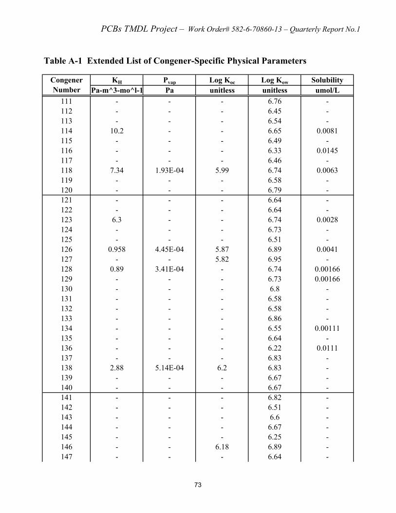
PCBs TMDL Project – Work Order# 582-6-70860-13 – Quarterly Report No.1
Table A-1 Extended List of Congener-Specific Physical Parameters
Congener Number
KH Pvap Log Koc Log Kow Solubility Pa-m^3-mo^l-1 Pa unitless unitless umol/L
111 - - - 6.76 -112 - - - 6.45 -113 - - - 6.54 -114 10.2 - - 6.65 0.0081 115 - - - 6.49 -116 - - - 6.33 0.0145 117 - - - 6.46 -118 7.34 1.93E-04 5.99 6.74 0.0063 119 - - - 6.58 -120 - - - 6.79 -121 - - - 6.64 -122 - - - 6.64 -123 6.3 - - 6.74 0.0028 124 - - - 6.73 -125 - - - 6.51 -126 0.958 4.45E-04 5.87 6.89 0.0041 127 - - 5.82 6.95 -128 0.89 3.41E-04 - 6.74 0.00166 129 - - - 6.73 0.00166 130 - - - 6.8 -131 - - - 6.58 -132 - - - 6.58 -133 - - - 6.86 -134 - - - 6.55 0.00111 135 - - - 6.64 -136 - - - 6.22 0.0111 137 - - - 6.83 -138 2.88 5.14E-04 6.2 6.83 -139 - - - 6.67 -140 - - - 6.67 -141 - - - 6.82 -142 - - - 6.51 -143 - - - 6.6 -144 - - - 6.67 -145 - - - 6.25 -146 - - 6.18 6.89 -147 - - - 6.64 -
73

PCBs TMDL Project – Work Order# 582-6-70860-13 – Quarterly Report No.1
Table A-1 Extended List of Congener-Specific Physical Parameters
Congener Number
KH Pvap Log Koc Log Kow Solubility Pa-m^3-mo^l-1 Pa unitless unitless umol/L
148 - - 5.95 6.73 -149 - 1.12E-03 6.05 6.67 -150 - - - 6.32 -151 - - 6.02 6.64 -152 - - - 6.22 -153 6.5 8.34E-04 6.19 6.92 0.00236 154 17.34 - - 6.76 -155 - - - 6.41 0.0083 156 6.8 2.15E-04 - 7.18 0.003 157 24.9 - - 7.18 0.0008 158 - - - 7.02 -159 - - - 7.24 -160 - - - 6.93 -161 - - - 7.08 -162 - - - 7.24 -163 - - - 6.99 -164 - - - 7.02 -165 - - - 7.05 -166 - - - 6.93 -167 10.4 3.05E-04 - 7.27 0.003 168 - - - 7.11 -169 8.6 1.82E-06 - 7.42 0.00036 170 0.128 - - 7.27 -171 - - - 7.11 0.00506 172 - - - 7.33 -173 - - - 7.02 -174 - - 6.3 7.11 -175 - - - 7.17 -176 - - - 6.76 -177 - - 6.35 7.08 -178 - - - 7.14 -179 - - - 6.73 -180 0.425 1.45E-04 6.37 7.36 -181 - - - 7.11 -182 - - - 7.2 -183 - 5.06E-04 6.32 7.2 -184 - - - 6.85 -
74

PCBs TMDL Project – Work Order# 582-6-70860-13 – Quarterly Report No.1
Table A-1 Extended List of Congener-Specific Physical Parameters
Congener Number
KH Pvap Log Koc Log Kow Solubility Pa-m^3-mo^l-1 Pa unitless unitless umol/L
185 - - - 7.11 0.00114 186 - - - 6.69 -187 3.034 - - 7.17 -188 15.77 - - 6.82 -189 25.1 - - 7.71 -190 - - - 7.46 -191 - - - 7.55 -192 - - - 7.52 -193 - - - 7.52 -194 - - - 7.8 -195 0.079 - - 7.56 -196 - - - 7.65 -197 - 1.87E-04 - 7.3 -198 - - - 7.62 -199 - - - 7.2 -200 - - - 7.27 -201 1.069 - - 7.62 -202 - - - 7.24 -203 - 1.30E-04 - 7.65 -204 - - - 7.3 -205 - - - 8 -206 - - - 8.09 -207 - - - 7.74 -208 - - - 7.71 -209 - - - 8.18 -
Sources Used: 1) Henry's Law Constants (KH) - Bamford, Poster and Baker, 2000,Fang, Chu and Hong, 2006 2) Vapor Pressure (Pvap)- Bidleman, 1984,Paasivirta, Sinkkonen, Mikkelson, Rantio and Wania, 1999 3) Sorption Partition Coefficients (Log Koc) - Hansen, Paya-Perez, Rahmanet al, 1999 4) Octanol-Water Coefficients (Kow) - Hawker and Connell, 1988 5) Solubility - Huang and Hong, 2002,Mackay, Shiu and Ma, 1992
Notes: 1) A '-' indicates that data was not supplied for that congener for that particular constant. 2) Congener 0 is the unchlorinated biphenyl molecule and is not technically a PCB. However, many sources
include the physical values for biphenyl to see structure-property relationship trends better.
75

PCBs TMDL Project – Work Order# 582-6-70860-13 –Quarterly Report No.1
APPENDIX B
PCB DATASET FROM DIOXIN TMDL PROJECT SAMPLING
76

PCBs TMDL Project - Contract# 582-6-70860/Work Order# 582-6-70860-13 - Quarterly Report No. 1
Table B-1 Total PCB Concentrations in Water (ng/L)
Station ID Date Volume (L) PCB 8 PCB 30/18 PCB 28/20 PCB 44/47/65 PCB 52 PCB 66 PCB 77
PCB 113/90/101 PCB 105 PCB 118 PCB 126 PCB 128/166
PCB 138/163/129 PCB 153/168 PCB 169 PCB 170
PCB 193/180 PCB 187 Total PCBsa Total PCBsb
Average Total PCBsb,c
Summer 2002 13343 08/20/2002 706 0.0051 0.0242 0.0361 0.0439 0.0595 0.0292 0.0034 0.0453 0.0105 0.0238 < 0.0003 0.0053 0.0357 0.0279 < 0.0001 0.0096 0.0174 0.0133 0.3906 0.3905 0.3905 13344 08/21/2002 709 < 0.0069 0.0271 0.0324 0.0969 0.1368 0.0472 0.0033 0.0733 0.0104 0.0228 < 0.0003 0.0048 0.0367 0.0310 < 0.0003 0.0072 0.0141 0.0120 0.5625 0.5613 0.5613 16496 08/22/2002 731 < 0.0082 0.0341 0.0315 0.0821 0.1081 0.0369 0.0038 0.0534 0.0118 0.0264 < 0.0003 0.0059 0.0397 0.0354 < 0.0003 0.0081 0.0161 0.0131 0.5135 0.5119 0.5119 13342 08/23/2002 509 0.0194 0.0477 0.0509 0.0974 0.1259 0.0373 0.0037 0.0747 0.0136 0.0403 < 0.0003 0.0067 0.0511 0.0511 < 0.0001 0.0106 0.0208 0.0181 0.6695 0.6693 0.6693 13337 08/24/2002 524 0.0202 0.0424 0.0443 0.0916 0.1164 0.0410 0.0036 0.0687 0.0145 0.0399 < 0.0003 0.0076 0.0553 0.0553 < 0.0003 0.0141 0.0248 0.0197 0.6598 0.6595 0.6595 13309 08/25/2002 532 0.0201 0.0303 0.0306 0.0545 0.0677 0.0289 0.0024 0.0545 0.0100 0.0252 < 0.0002 0.0048 0.0391 0.0427 < 0.0002 0.0084 0.0162 0.0154 0.4509 0.4508 0.4508 16618 08/26/2002 505 0.0174 0.0566 0.0554 0.0905 0.1164 0.0457 0.0044 0.0673 0.0147 0.0327 < 0.0002 0.0059 0.0455 0.0475 < 0.0001 0.0101 0.0188 0.0166 0.6459 0.6458 0.6458 13338 08/26/2002 544 0.0145 0.0368 0.0349 0.0717 0.0938 0.0379 0.0035 0.0662 0.0143 0.0369 < 0.0004 0.0086 0.0607 0.0588 < 0.0005 0.0142 0.0256 0.0222 0.6011 0.6006 0.6006 11264 08/27/2002 268 0.0247 0.1463 0.1392 0.2698 0.3108 0.1377 0.0125 0.1493 0.0381 0.0754 < 0.0007 0.0142 0.1045 0.0896 < 0.0004 0.0250 0.0560 0.0313 1.6247 1.6241 1.6241 15979 08/27/2002 522 0.0213 0.0971 0.0950 0.1759 0.2107 0.0715 0.0077 0.1073 0.0259 0.0536 < 0.0005 0.0126 0.0900 0.0747 < 0.0004 0.0222 0.0490 0.0274 1.1426 1.1422 1.1422 11270 08/28/2002 508 0.0224 0.1128 0.1157 0.2087 0.2480 0.0846 0.0089 0.1181 0.0325 0.0669 < 0.0005 0.0138 0.0984 0.0807 < 0.0004 0.0224 0.0508 0.0278 1.3132 1.3128 1.3128 15908 08/29/2002 503 0.0133 0.0199 0.0264 0.0501 0.0791 0.0203 0.0016 0.0402 0.0064 0.0181 < 0.0003 0.0038 0.0322 0.0332 < 0.0003 0.0066 0.0149 0.0107 0.3771 0.3768 0.3768 13336 08/29/2002 523 < 0.0069 0.0327 0.0424 < 0.0765 0.1128 0.0346 0.0033 0.0574 0.0117 0.0300 < 0.0004 0.0071 0.0518 0.0501 < 0.0003 0.0120 0.0260 0.0182 0.5446 0.5150 0.5150 11252 08/30/2002 703 0.0121 0.0259 0.0299 0.0637 0.0920 0.0245 0.0023 0.0384 0.0077 0.0188 < 0.0002 0.0038 0.0284 0.0282 < 0.0001 0.0062 0.0138 0.0101 0.4059 0.4057 0.4057 17971 08/31/2002 522 0.0121 0.0456 0.0492 0.0931 0.1374 0.0354 0.0037 0.0529 0.0113 0.0259 < 0.0004 0.0044 0.0370 0.0356 < 0.0003 0.0080 0.0167 0.0119 0.5804 0.5801 0.5801 13363 08/31/2002 560 < 0.0037 0.0152 0.0216 0.0350 0.0543 0.0163 0.0011 0.0334 0.0048 0.0145 < 0.0003 0.0028 0.0225 0.0248 < 0.0004 0.0046 0.0104 0.0086 0.2719 0.2696 0.2696 11200 09/02/2002 508 0.0091 0.0102 0.0122 0.0110 0.0122 0.0047 0.0004 0.0181 0.0035 0.0075 < 0.0003 0.0032 0.0240 0.0220 < 0.0002 0.0079 0.0213 0.0126 0.1803 0.1800 0.1800 16622 09/02/2002 529 < 0.0127 0.0195 0.0204 0.0195 0.0420 0.0093 0.0009 0.0236 0.0041 0.0093 < 0.0002 0.0023 0.0174 0.0155 < 0.0005 0.0054 0.0129 0.0087 0.2219 0.2198 0.2198 11292 09/03/2002 610 0.0170 0.0682 0.1098 0.0951 0.1066 0.0377 0.0041 0.0607 0.0182 0.0385 < 0.0005 0.0098 0.0770 0.0646 < 0.0003 0.0234 0.0485 0.0300 0.8098 0.8094 0.9489
11292-dup 09/03/2002 716 < 0.0190 0.1345 0.1480 0.1480 0.1592 0.0482 0.0059 0.0838 0.0216 0.0461 < 0.0005 0.0115 0.0894 0.0712 < 0.0001 0.0240 0.0490 0.0307 1.0896 1.0883 11280 09/04/2002 501 < 0.0172 0.0828 0.1038 0.1651 0.2371 0.0547 0.0059 0.0918 0.0224 0.0499 < 0.0003 0.0098 0.0699 0.0539 < 0.0002 0.0172 0.0337 0.0246 1.0383 1.0364 1.0364 14560 09/04/2002 622 < 0.0058 0.0087 0.0130 0.0235 0.0341 0.0109 0.0007 0.0246 0.0037 0.0111 < 0.0002 0.0024 0.0186 0.0235 < 0.0002 0.0038 0.0072 0.0079 0.1989 0.1980 0.1980 13341 09/05/2002 509 < 0.0122 0.0187 0.0279 0.0395 0.0585 0.0193 0.0014 0.0432 0.0092 0.0253 < 0.0002 0.0061 0.0472 0.0424 < 0.0001 0.0120 0.0236 0.0196 0.4052 0.4039 0.4039 13339 09/06/2002 304 < 0.0148 0.0365 0.0497 0.0849 0.1138 0.0378 0.0042 0.0720 0.0171 0.0428 < 0.0004 0.0093 0.0734 0.0635 < 0.0002 0.0168 0.0329 0.0306 0.7004 0.7000 0.7000 13340 09/06/2002 367 < 0.0124 0.0175 0.0234 0.0338 0.0474 0.0166 0.0012 0.0398 0.0076 0.0221 < 0.0002 0.0050 0.0422 0.0373 < 0.0002 0.0092 0.0180 < 0.0036 0.3373 0.3370 0.3370 16213 09/10/2002 557 0.0124 0.0110 0.0151 0.0230 0.0293 0.0145 0.0011 0.0294 0.0055 0.0160 < 0.0002 0.0035 0.0307 0.0334 < 0.0002 0.0064 0.0133 0.0115 0.2561 0.2560 0.2560 13589 09/10/2002 512 0.0141 0.0125 0.0154 0.0195 0.0275 0.0104 0.0015 0.0248 0.0041 0.0117 < 0.0002 0.0022 0.0213 0.0227 < 0.0001 0.0040 0.0092 0.0078 0.2089 0.2088 0.2088 11193 09/11/2002 508 0.0531 0.0262 0.0346 0.0360 0.0630 0.0179 0.0017 0.0531 0.0150 0.0368 < 0.0001 0.0084 0.0539 0.0415 < 0.0001 0.0106 0.0203 0.0154 0.4876 0.4875 0.4875 15464 09/11/2002 318 < 0.0101 0.0116 0.0189 0.0201 0.0283 0.0126 0.0010 0.0267 0.0049 0.0138 < 0.0002 0.0028 0.0223 0.0252 < 0.0003 0.0053 0.0099 0.0099 0.2220 0.2200 0.2200 11261 09/12/2002 532 0.0141 0.0419 0.0568 0.1028 0.1276 0.0445 0.0047 0.0602 0.0160 0.0348 < 0.0003 0.0068 0.0461 0.0382 < 0.0001 0.0105 0.0197 0.0154 0.6402 0.6400 0.6400 11287 09/12/2002 508 0.0077 0.0317 0.0498 0.0537 0.0626 0.0191 0.0028 0.0400 0.0108 0.0226 0.0003 0.0065 0.0459 0.0360 < 0.0002 0.0114 0.0222 0.0157 0.4391 0.4391 0.4391 16499 09/13/2002 509 0.0086 0.0291 0.0344 0.0741 0.1055 0.0275 0.0031 0.0530 0.0108 0.0271 < 0.0003 0.0059 0.0464 0.0409 < 0.0001 0.0110 0.0218 0.0196 0.5190 0.5188 0.5183
16499-dup 09/13/2002 529 0.0091 0.0308 0.0365 0.0756 0.1021 0.0285 0.0030 0.0529 0.0108 0.0268 < 0.0002 0.0055 0.0463 0.0408 < 0.0001 0.0102 0.0198 0.0187 0.5178 0.5177
77

PCBs TMDL Project - Contract# 582-6-70860/Work Order# 582-6-70860-13 - Quarterly Report No. 1
Table B-1 Total PCB Concentrations in Water (ng/L) - Cont'd
Station ID Date Volume (L) PCB 8 PCB 30/18 PCB 28/20 PCB 44/47/65 PCB 52 PCB 66 PCB 77
PCB 113/90/101 PCB 105 PCB 118 PCB 126 PCB 128/166
PCB 138/163/129 PCB 153/168 PCB 169 PCB 170
PCB 193/180 PCB 187 Total PCBsa Total PCBsb
Average Total PCBsb,c
Fall 2002 11261 10/21/2002 422 0.0175 0.0429 0.0453 0.0995 0.1173 0.0377 0.0030 0.0382 0.0100 0.0258 < 0.0002 0.0047 0.0469 0.0419 < 0.0001 0.0065 0.0133 0.0107 0.5613 0.5611 0.5611 13341 10/24/2002 651 0.0060 0.0152 0.0209 0.0402 0.0482 0.0172 0.0014 0.0353 0.0061 0.0187 < 0.0002 0.0055 0.0584 0.0424 < 0.0002 0.0120 0.0252 0.0221 0.3751 0.3749 0.3749 13342 10/29/2002 712 0.0150 0.0725 0.0742 0.1053 0.1320 0.0479 0.0041 0.0618 0.0147 0.0344 0.0002 0.0070 0.0520 0.0421 < 0.0002 0.0108 0.0218 0.0176 0.7135 0.7134 0.7134 16499 10/30/2002 715 < 0.0170 0.1930 0.2154 0.3301 0.3455 0.1399 0.0080 0.1622 0.0340 0.0713 0.0004 0.0151 0.1189 0.0881 < 0.0001 0.0215 0.0400 0.0338 1.8341 1.8340 1.8340 13363 10/31/2002 727 0.0296 0.1076 0.1188 0.1513 0.1967 0.0624 0.0044 0.0605 0.0168 0.0362 < 0.0003 0.0061 0.0426 0.0316 < 0.0003 0.0074 0.0154 0.0133 0.9011 0.9009 0.9009 15979 11/01/2002 662 0.0826 0.3310 0.3580 0.3988 0.5181 0.1903 0.0136 0.1918 0.0468 0.1073 0.0005 0.0189 0.1360 0.0967 < 0.0003 0.0255 0.0491 0.0409 2.6061 2.6059 2.6059 13336 11/05/2002 570 0.0256 0.0542 0.0793 0.0860 0.0935 0.0467 0.0042 0.0526 < 0.0191 0.0386 < 0.0007 0.0070 0.0491 0.0404 < 0.0004 0.0158 0.0232 0.0156 0.6463 0.6407 0.6407 11280 11/06/2002 703 0.0523 0.0737 0.1127 0.0825 0.0896 0.0390 0.0044 0.0626 0.0218 0.0498 < 0.0010 0.0108 0.0811 0.0612 < 0.0012 0.0283 0.0418 0.0262 0.8388 0.8377 0.8377 11292 11/07/2002 722 0.0342 0.0479 0.0573 0.0542 0.0686 0.0229 < 0.0029 0.0429 0.0130 0.0291 < 0.0005 0.0089 0.0568 0.0429 < 0.0005 0.0169 0.0321 0.0233 0.5537 0.5525 0.5525 13344 11/08/2002 711 0.0115 0.0222 0.0322 0.0406 0.0489 0.0194 0.0016 0.0328 0.0080 0.0214 < 0.0002 0.0035 0.0267 0.0245 < 0.0002 0.0063 0.0097 0.0080 0.3177 0.3175 0.3175 13355 11/11/2002 498 0.0249 0.0325 0.0434 0.0456 0.0546 0.0217 0.0020 0.0450 < 0.0116 0.0267 < 0.0003 0.0058 0.0390 0.0349 < 0.0004 0.0139 0.0197 0.0133 0.4314 0.4275 0.4275 13338 11/12/2002 476 0.0475 0.0525 0.0624 0.0855 0.1113 0.0439 0.0034 0.0840 0.0197 0.0462 < 0.0006 0.0101 0.0714 0.0588 < 0.0007 0.0166 0.0313 0.0269 0.7723 0.7717 0.7717 14560 11/13/2002 703 0.0199 0.0245 0.0253 0.0344 0.0458 0.0158 < 0.0019 0.0286 0.0060 0.0149 < 0.0005 0.0030 0.0202 0.0185 < 0.0005 0.0046 0.0087 0.0077 0.2793 0.2778 0.2778 11252 11/14/2002 706 0.0174 0.0317 0.0351 0.0452 0.0557 0.0239 < 0.0017 0.0395 0.0067 0.0174 < 0.0004 0.0027 0.0225 0.0217 < 0.0005 0.0052 0.0101 0.0091 0.3457 0.3449 0.3296
11252-dup 11/14/2002 707 0.0163 0.0272 0.0294 0.0446 0.0569 0.0231 < 0.0023 0.0359 0.0061 0.0165 < 0.0003 0.0025 0.0182 0.0170 < 0.0005 0.0047 0.0088 0.0072 0.3158 0.3142 17971 11/18/2002 708 0.0116 0.0407 0.0531 0.0689 0.0922 0.0410 0.0030 0.0404 0.0109 0.0271 < 0.0002 0.0045 0.0339 0.0297 < 0.0002 0.0075 0.0133 0.0110 0.4890 0.4888 0.4803
17971-dup 11/18/2002 711 0.0105 0.0406 0.0450 0.0727 0.0882 0.0345 < 0.0030 0.0457 0.0110 0.0248 < 0.0004 0.0048 0.0323 0.0284 < 0.0007 0.0072 0.0135 0.0105 0.4729 0.4719 15464 11/19/2002 702 0.0083 0.0111 0.0138 0.0158 0.0222 0.0108 0.0007 0.0131 0.0030 0.0091 < 0.0002 0.0017 0.0124 0.0138 < 0.0002 0.0032 0.0057 0.0053 0.1501 0.1500 0.1500 11193 11/20/2002 709 0.0395 0.0312 0.0389 0.0377 0.0508 0.0186 0.0015 0.0339 0.0094 0.0264 < 0.0002 0.0042 0.0319 0.0250 < 0.0001 0.0055 0.0124 0.0093 0.3762 0.3761 0.3761 11200 11/21/2002 707 0.0122 0.0154 0.0191 0.0113 0.0137 0.0045 < 0.0004 0.0089 0.0021 0.0055 < 0.0002 0.0012 0.0091 0.0085 < 0.0001 0.0020 0.0050 0.0042 0.1232 0.1229 0.1229
Spring 2003 11264 06/02/2003 702 < 0.0214 0.1142 0.0876 0.2236 0.2835 0.0912 < 0.0048 0.1168 0.0211 0.0456 < 0.0023 0.0080 0.0570 0.0442 < 0.0010 0.0137 0.0239 0.0205 1.1760 1.1717 1.1398
11264-dup 06/02/2003 701 < 0.0190 0.1070 0.0827 0.2254 0.2568 0.0827 0.0056 0.1084 0.0197 0.0414 < 0.0022 0.0083 0.0571 0.0428 < 0.0011 0.0126 0.0227 0.0193 1.1113 1.1080 11280 06/11/2003 700 < 0.0191 0.1089 0.1043 0.1571 0.1729 0.0504 0.0061 0.0786 0.0203 0.0457 < 0.0004 0.0091 0.0714 0.0586 < 0.0002 0.0150 0.0296 0.0204 0.9670 0.9658 0.9658 11287 06/17/2003 706 0.2732 0.1262 0.1418 0.1204 < 0.1119 0.0524 0.0081 0.1020 0.0382 0.0708 < 0.0009 0.0239 0.1700 0.1218 < 0.0004 0.0482 0.0836 0.0510 1.5442 1.5435 1.5435 11270 06/18/2003 702 0.0387 0.1477 0.1809 0.2821 0.3162 0.1182 0.0161 0.1524 0.0484 0.0983 < 0.0010 0.0209 0.1510 0.1111 < 0.0003 0.0308 0.0568 0.0409 1.8114 1.8110 1.8110
Total PCB concentration calculated as the sum of the 18 congeners recommended by NOAA If either the dissolved or suspended concentration was non-detected, the total concentration in water is reported here as less than the sum of the detected concentration and the MDL for the non-detected phase. If a congener was non-detected in both phases, the total concentration in wat is reported as less than the sum of the MDLs for both phases. a Non-detects assumed to be 1/2 detection limit b Non-detects assumed to be zero c Average of duplicate samples, otherwise concentration of a single sample Exceeds the WQS (0.885 ng/L)
78

PCBs TMDL Project - Contract# 582-6-70860/Work Order# 582-6-70860-13 - Quarterly Report No. 1
Table B-2 PCB Concentrations in Sediment (ng/kg-dry wt.)
Station ID Date PCB 8 PCB 30/18 PCB 28/20 PCB 44/47/65 PCB 52 PCB 66 PCB 77 PCB 113/90/101 PCB 105 PCB 118 PCB 126 PCB 128/166 PCB 138/163/129 PCB 153/168 PCB 169 PCB 170 PCB 193/180 PCB 187 Total PCBsa Total PCBsb Average Total
PCBsb,c
Summer 2002 11272 07/25/2002 87 78.6 190 241 247 238 < 48.1 227 88.6 223 < 48.1 < 48.1 283 257 < 48.1 92.2 213 132 2693.6 2597.4 2597.4 11298 07/29/2002 579 767 1780 2710 3200 1400 271 4550 1230 2800 < 47.3 880 6370 4440 < 47.3 2750 6130 4040 43944.3 43897.0 43897.0 11274 07/30/2002 9030 8670 22300 7580 7400 16800 2100 8570 5290 9890 139 2230 11600 7330 < 47.9 1590 3530 1700 125773.0 125749.0 125749.0 11111 07/31/2002 215 90.3 336 189 195 119 50 275 133 372 < 49.5 72.9 545 511 < 49.5 152 287 183 3774.7 3725.2 3725.2 11092 08/01/2002 578 711 1670 1110 1270 1080 122 1670 488 1330 < 98.7 318 1580 1490 < 98.7 485 1060 670 15730.7 15632.0 15632.0 11258 08/01/2002 < 48.8 < 48.8 72.4 57.2 64 < 48.8 < 48.8 56.3 < 48.8 < 48.8 < 48.8 < 48.8 51.4 < 48.8 < 48.8 < 48.8 < 48.8 < 48.8 618.5 301.3 301.3 13340 08/06/2002 < 49.9 121 < 49.9 < 49.9 < 49.9 < 49.9 < 49.9 1740 300 1060 < 49.9 239 1580 1410 < 49.9 575 1230 828 9282.6 9083.0 9083.0 13341 08/06/2002 127 122 339 536 702 < 49.5 53.9 1100 292 834 < 49.5 258 1800 1580 < 49.5 455 1040 522 9835.2 9760.9 9760.9 11193 08/08/2002 1090 75.7 259 326 585 283 < 49.6 934 369 976 < 49.6 217 1480 1060 < 49.6 321 663 322 9035.1 8960.7 8960.7 11347 08/12/2002 97.8 136 400 698 1070 775 157 6520 3940 8260 58.1 1590 9000 4940 < 49.9 1270 1970 910 41816.9 41791.9 41791.9 11382 08/12/2002 < 49.8 370 1130 1290 1550 809 178 2190 851 1600 < 49.8 569 3150 1970 < 49.8 858 1810 1010 19409.7 19335.0 19335.0 11305 08/13/2002 246 429 939 1740 1130 103 102 2200 559 1250 < 48.6 496 4630 3840 < 48.6 1980 4720 2100 26512.6 26464.0 27159.0
11305-dup 08/13/2002 315 490 1120 2090 1340 148 137 2370 679 1580 < 49.7 735 5700 4870 < 49.7 1460 3150 1670 27903.7 27854.0 13337 08/14/2002 326 234 929 1050 1120 < 49.6 103 926 323 830 < 49.6 175 1210 1010 < 49.6 293 631 380 9614.4 9540.0 9540.0 13363 08/16/2002 < 49.1 < 49.1 < 49.1 < 49.1 < 49.1 < 49.1 < 49.1 < 49.1 < 49.1 < 49.1 < 49.1 < 49.1 < 49.1 < 49.1 56 < 49.1 < 49.1 < 49.1 473.4 56.0 56.0 13589 08/16/2002 < 50.5 < 50.5 88.7 93.6 121 77.2 < 50.5 < 50.5 < 50.5 < 50.5 < 50.5 < 50.5 165 126 < 50.5 < 50.5 < 50.5 < 50.5 974.5 671.5 671.5 15464 08/16/2002 < 49.6 < 49.6 69.9 55.2 56 54.6 < 49.6 < 49.6 < 49.6 < 49.6 < 49.6 < 49.6 54.7 52.2 < 49.6 < 49.6 < 49.6 < 49.6 640.2 342.6 342.6 17970 08/18/2002 < 48.6 < 48.6 88.7 57.9 69.4 69.3 < 48.6 69.1 < 48.6 63.6 < 48.6 < 48.6 102 95 < 48.6 < 48.6 < 48.6 < 48.6 858.0 615.0 615.0 13355 08/18/2002 < 45 < 45 88.7 50.7 60.3 65.6 < 45 86.4 < 45 72.5 < 45 < 45 130 106 < 45 < 45 < 45 < 45 885.2 660.2 660.2 11261 08/19/2002 92.7 112 238 390 433 278 < 49.6 460 123 283 < 49.6 92.5 708 715 < 49.6 238 571 404 5212.6 5138.2 5138.2 13343 08/20/2002 68.2 96.2 253 245 282 247 < 49.1 236 105 235 < 49.1 65.5 399 284 < 49.1 93.8 191 121 2995.4 2921.7 2921.7 11264 08/20/2002 646 921 1830 3170 3830 2370 257 4910 1890 4260 < 49 1090 6030 4080 < 49 892 1620 834 38679.0 38630.0 38630.0 16618 08/20/2002 550 229 352 469 669 317 < 43.9 677 186 564 < 43.9 84.2 601 468 < 43.9 153 319 194 5898.1 5832.2 5832.2 16496 08/21/2002 198 165 547 969 1140 949 107 1700 325 947 < 47.3 239 1550 1520 < 47.3 < 47.3 987 650 12064.0 11993.0 11993.0 11302 08/21/2002 875 766 1790 1090 1040 < 48.8 157 1170 564 1200 < 48.8 346 2570 1870 < 48.8 548 1220 606 15885.2 15812.0 15812.0 13338 08/21/2002 746 1100 1990 3500 3820 1700 233 3990 902 2370 < 48.3 501 3690 3370 < 48.3 910 1960 1380 32210.3 32162.0 33420.5
13338-dup 08/21/2002 845 1040 2110 3840 4090 3060 243 3910 940 2490 < 46.8 490 3580 3250 < 46.8 981 2190 1620 34725.8 34679.0 13342 08/21/2002 197 221 632 1300 1510 773 122 2030 446 1170 < 48.7 245 1720 1500 < 48.7 620 1130 833 14497.7 14449.0 14449.0 13344 08/21/2002 212 202 608 845 969 939 128 1120 394 1040 < 48.7 252 1770 1570 < 48.7 399 693 585 11774.7 11726.0 11726.0 13339 08/22/2002 238 247 643 1230 1480 694 118 1880 410 1100 < 47.1 275 1920 1740 < 47.1 522 1170 1060 14774.1 14727.0 14727.0 16499 08/22/2002 304 315 783 1750 1960 1240 131 2340 524 1250 < 46.9 353 2840 2970 < 46.9 1060 2550 1870 22286.9 22240.0 22240.0 17971 08/24/2002 275 267 808 2270 1560 907 174 2600 643 1680 < 49.7 501 5270 5620 < 49.7 2630 5590 3260 34104.7 34055.0 35217.0
17971-dup 08/24/2002 208 263 862 2980 2250 1070 179 3220 652 1730 < 44.8 645 5860 6110 < 44.8 2220 4960 3170 36423.8 36379.0 11287 08/26/2002 667 684 1380 1700 1730 880 154 2120 602 1400 < 49.2 382 2600 2110 < 49.2 763 1620 1120 19961.2 19912.0 19912.0 11252 08/27/2002 < 47.3 52.3 131 135 147 149 < 47.3 80 85 63.1 < 47.3 < 47.3 86 83 < 47.3 < 47.3 < 47.3 < 47.3 1200.6 1011.4 684.2
11252-dup 08/27/2002 < 48.9 < 48.9 91.3 71.2 77.2 60 < 48.9 57.3 < 48.9 < 48.9 < 48.9 < 48.9 < 48.9 < 48.9 < 48.9 < 48.9 < 48.9 < 48.9 674.9 357.0 13336 08/27/2002 116 106 326 231 260 375 < 47.8 387 132 446 < 47.8 69.8 531 678 < 47.8 147 274 202 4352.5 4280.8 4324.2
13336-dup 08/27/2002 152 119 362 340 361 470 < 49.4 416 107 388 < 49.4 53.5 396 566 < 49.4 147 286 204 4441.6 4367.5 11273 08/28/2002 20200 64300 124000 265000 306000 171000 17000 105000 45800 83700 423 12900 82600 63300 244 13800 25500 17400 1418167.0 1418167.0 1445307.7
11273-dup 08/28/2002 24700 61500 132000 264000 317000 161000 19000 140000 48800 80200 669 12600 81100 61300 79.3 16700 32300 19500 1472448.3 1472448.3 11270 08/28/2002 2960 2560 6170 11200 10900 8660 458 10200 1540 6320 < 49 987 6770 6730 < 49 1210 2660 2040 81414.0 81365.0 81365.0 11280 08/29/2002 < 1490 2210 4830 8420 8220 4070 580 11000 2660 6950 < 97.7 1370 11500 10500 < 97.7 4950 11700 6600 96402.7 95560.0 95560.0 13309 08/30/2002 67.5 87.8 196 197 225 224 < 44.6 244 97.7 240 < 44.6 53.6 325 249 < 44.6 57.7 118 69.1 2518.3 2451.4 2451.4 14560 08/30/2002 132 157 378 450 460 496 < 46.5 531 186 487 < 46.5 124 879 800 < 46.5 226 477 306 6158.8 6089.0 6089.0 16622 09/03/2002 84.7 152 394 619 728 368 51.6 836 210 478 < 48.5 123 699 670 < 48.5 185 451 345 6442.8 6394.3 6394.3 11200 09/03/2002 < 45.6 < 45.6 88.9 46.6 53.1 58.3 < 45.6 50.2 < 45.6 46.9 < 45.6 < 45.6 78.1 62.3 < 45.6 < 45.6 < 45.6 < 45.6 712.4 484.4 419.8
11200-dup 09/03/2002 < 47.9 < 47.9 96.2 < 47.9 52.1 60 < 47.9 < 47.9 < 47.9 < 47.9 < 47.9 < 47.9 75.1 71.7 < 47.9 < 47.9 < 47.9 < 47.9 666.5 355.1 15979 09/04/2002 11300 4310 6480 13300 21000 7710 956 21300 5330 14800 63.7 2900 22400 20000 < 46.8 4840 11300 6970 174983.1 174959.7 154092.0
15979-dup 09/04/2002 9060 3290 5240 10500 15800 5640 735 16900 3990 9020 59.2 2100 17600 15600 < 45.9 3640 8480 5570 133247.2 133224.2 11292 09/05/2002 1010 2090 5020 8410 6320 3480 523 8120 2260 5530 54.5 1850 15400 14200 < 49.7 4750 10300 7270 96612.4 96587.5 96587.5 11300 09/05/2002 4900 4680 10300 17800 23300 10200 1960 43500 9750 25500 293 8190 55800 48500 57.8 9890 21800 15700 312120.8 312120.8 311932.3
11300-dup 09/05/2002 8170 6810 13700 20100 25600 10900 1880 39000 9480 24000 299 7750 53800 46300 54.7 9000 20000 14900 311743.7 311743.7 15908 09/11/2002 < 46.9 53.5 126 127 < 46.9 74 < 46.9 151 < 46.9 83.9 < 46.9 < 46.9 81.1 88.3 < 46.9 < 46.9 47.5 51 1070.9 883.3 883.3 16213 09/11/2002 126 66.2 167 245 290 194 < 45.7 428 79.9 463 < 45.7 54.7 376 482 < 45.7 97.2 198 204 3539.6 3471.0 3471.0
Fall 2002 13338 10/22/2002 200 209 517 693 777 568 63.9 820 247 634 < 48.8 131 872 795 < 48.8 261 536 373 7745.7 7696.9 7696.9 13336 10/22/2002 154 174 448 656 746 513 58.9 845 236 613 < 47.5 139 988 907 < 47.5 299 626 421 7871.4 7823.9 7823.9 13340 10/23/2002 150 124 305 645 906 528 57.7 1670 301 1130 < 45.8 244 1780 1730 < 45.8 574 1150 915 12255.5 12209.7 12209.7 11252 10/24/2002 92.2 82.4 222 291 330 272 < 47.2 397 103 299 < 47.2 59.3 387 402 < 47.2 123 240 201 3571.7 3500.9 3500.9
79

PCBs TMDL Project - Contract# 582-6-70860/Work Order# 582-6-70860-13 - Quarterly Report No. 1
17970 10/24/2002 56.6 65.3 157 159 204 146 < 48.7 215 49.8 167 < 48.7 < 48.7 156 143 < 48.7 < 48.7 63.9 49.7 1754.1 1632.3 1632.3
80

PCBs TMDL Project - Contract# 582-6-70860/Work Order# 582-6-70860-13 - Quarterly Report No. 1
Table B-2 PCB Concentrations in Sediment (ng/kg-dry wt.) - Cont'd
Station ID Date PCB 8 PCB 30/18 PCB 28/20 PCB 44/47/65 PCB 52 PCB 66 PCB 77 PCB 113/90/101 PCB 105 PCB 118 PCB 126 PCB 128/166 PCB 138/163/129 PCB 153/168 PCB 169 PCB 170 PCB 193/180 PCB 187 Total PCBsa Total PCBsb Average Total
PCBsb,c
16499 10/24/2002 172 172 404 863 1090 566 84.5 1630 300 802 < 39.9 197 2400 2980 < 39.9 1010 2580 2040 17330.4 17290.5 17290.5 11261 10/26/2002 104 114 281 498 573 411 55.7 611 195 487 < 48 92.5 592 488 < 48 192 381 255 5378.2 5330.2 5330.2 13344 10/27/2002 217 232 655 1160 1280 1070 131 1550 369 1200 < 46.1 219 1430 1460 < 46.1 420 828 664 12931.1 12885.0 12885.0 17971 10/28/2002 307 289 657 1160 1230 848 95.5 1330 317 956 < 48.3 190 1420 1340 < 48.3 460 935 656 12238.8 12190.5 12190.5 13342 10/30/2002 213 220 641 1290 1460 943 129 1560 457 1170 < 46.6 261 1810 1560 < 46.6 510 991 786 14047.6 14001.0 14001.0 11193 10/31/2002 694 87.6 241 448 653 312 52.8 1330 285 696 < 49.7 217 1710 1770 < 49.7 528 1240 921 11235.1 11185.4 11185.4 13363 11/06/2002 < 49.5 < 49.5 100 92.4 120 79.8 < 49.5 129 < 49.5 72.8 < 49.5 < 49.5 82.4 84.6 < 49.5 < 49.5 < 49.5 < 49.5 1008.5 761.0 761.0 15464 11/06/2002 < 48.3 < 48.3 97.4 67.1 77 61.9 < 48.3 62.5 < 48.3 < 48.3 < 48.3 < 48.3 < 48.3 < 48.3 < 48.3 < 48.3 < 48.3 < 48.3 679.9 365.9 365.9 11200 11/21/2002 < 50 < 50 76.3 < 50 < 50 < 50 < 50 < 50 < 50 < 50 < 50 < 50 < 50 < 50 < 50 < 50 < 50 < 50 501.3 76.3 76.3 11280 12/02/2002 107 2600 5050 7810 6480 4440 472 8480 2120 5490 < 49.9 1520 11700 11300 < 49.9 3750 9040 5300 85708.9 85659.0 103601.5
11280-dup 12/02/2002 2710 3630 6690 11600 9790 6120 641 13200 3230 8080 62.9 2040 14600 14100 < 48.5 5440 12300 7310 121568.2 121543.9 11292 12/10/2002 20900 33800 49500 59700 81300 45600 4620 110000 24500 47900 431 20800 189000 167000 82.3 54800 133000 74300 1117233.3 1117233.3 1117233.3
Spring 2003 11092 04/30/2003 1030 894 1730 1360 1500 736 111 1230 374 956 < 46.5 231 1750 1410 < 46.5 288 628 < 46.5 14297.8 14228.0 14228.0 11258 04/30/2003 222 358 664 819 851 770 79 633 231 557 < 47.7 116 793 674 < 47.7 214 460 278 7766.7 7719.0 7719.0 11272 04/30/2003 < 248 < 248 593 786 881 620 < 248 899 274 688 < 248 < 496 1240 1040 < 248 276 580 383 9128.0 8260.0 8260.0 11274 05/01/2003 1710 2110 4780 4560 4920 3700 520 2930 1390 2820 < 49.2 560 3200 2150 < 49.2 630 1340 772 38141.2 38092.0 41617.5
11274-dup 05/01/2003 1550 2030 4870 6290 6440 4070 491 3750 1600 3350 < 49 706 4360 2970 < 49 599 1320 747 45192.0 45143.0 11111 05/01/2003 136 111 279 266 309 203 < 47.6 296 72.6 221 < 47.6 < 95.2 353 383 < 47.6 78.2 149 114 3089.8 2970.8 2970.8 11302 05/01/2003 278 487 1150 1430 1460 969 < 239 1750 698 1500 < 239 499 3400 2600 < 239 831 1850 1050 20310.5 19952.0 19952.0 11298 05/02/2003 619 905 1710 2390 2770 1460 < 229 3830 1090 2380 < 229 815 5750 4210 < 229 1930 4240 2810 37252.5 36909.0 36909.0 11273 05/03/2003 11500 42000 80400 118000 134000 132000 11100 70000 23500 38200 539 7590 48600 39700 < 231 9990 20700 12200 800134.5 800019.0 810877.0
11273-dup 05/03/2003 11100 43300 79300 130000 144000 124000 11400 73000 23800 42400 615 8230 51500 40400 < 240 8990 18700 11000 821855.0 821735.0 11305 05/04/2003 < 795 916 1350 2950 1530 948 < 244 2990 884 2050 < 244 900 6140 4750 < 244 1660 3700 2050 33581.5 32818.0 32818.0 11347 05/04/2003 < 239 310 593 601 695 518 < 239 945 522 1140 < 239 < 478 1720 1160 < 239 394 761 418 10494.0 9777.0 9777.0 13339 05/04/2003 100 78.7 207 231 275 190 < 49.9 328 95.2 250 < 49.9 < 99.9 424 363 < 49.9 98.6 210 161 3136.3 3011.5 3011.5 11287 05/05/2003 486 1010 1880 1390 1340 458 71.4 1100 388 927 < 47.4 337 2260 1810 < 47.4 473 1060 685 15722.8 15675.4 15675.4 11382 05/05/2003 < 235 521 1220 1330 1510 630 < 235 1100 502 938 < 235 < 471 1580 1050 < 235 349 699 397 12531.5 11826.0 11826.0 11270 05/06/2003 335 431 939 1480 1570 1060 127 1020 505 1050 < 49.5 187 1130 847 < 49.5 294 626 369 12019.5 11970.0 11970.0 11280 05/06/2003 1110 1540 3490 5840 6260 3650 507 9030 2600 6630 < 241 1930 12500 9790 < 241 3060 6370 3590 78138.0 77897.0 77897.0 11292 05/06/2003 673 1180 2480 4260 3070 1920 208 4130 1020 2530 65.5 761 5120 4710 < 47.5 1760 4050 2180 40141.3 40117.5 40812.3 16618 05/06/2003 1090 1040 1600 2360 2840 2510 256 4180 998 2670 < 238 723 6230 5700 < 238 2080 4670 2560 41745.0 41507.0 23751.5 11261 05/11/2003 282 149 368 577 703 158 55.9 645 229 563 < 46.4 122 750 639 < 46.4 188 374 193 6042.3 5995.9 5995.9 13342 05/11/2003 197 194 511 979 1150 742 110 1270 356 923 < 48.8 220 1390 1290 < 48.8 471 904 569 11324.8 11276.0 11276.0 13343 05/11/2003 84 97.2 274 359 428 297 < 48.7 382 126 299 < 48.7 < 97.4 484 431 < 48.7 129 248 173 3933.0 3811.2 3811.2 16496 05/11/2003 458 514 1230 2290 2480 1530 136 2100 626 1570 < 50.3 367 2430 2330 < 50.3 701 1510 833 21155.3 21105.0 21105.0 13309 05/12/2003 < 47.8 < 47.8 70.2 < 57.3 < 47.8 < 47.8 < 47.8 < 47.8 < 47.8 < 47.8 < 47.8 < 95.5 < 47.8 < 57.3 < 47.8 < 47.8 < 47.8 < 47.8 509.9 70.2 70.2 14560 05/12/2003 50.9 < 48.9 75 66.9 97.3 55.5 < 48.9 158 < 48.9 125 < 48.9 < 97.8 132 117 < 48.9 < 48.9 < 48.9 < 48.9 1122.1 877.6 877.6 15464 05/12/2003 65.2 56.1 122 87 93.5 98.6 < 50 74.7 < 50 58.6 < 50 < 100 65.8 75.5 < 50 < 50 < 50 < 50 1022.0 797.0 797.0 16213 05/12/2003 62.9 58.6 139 106 126 90.3 < 48.8 114 < 48.8 73 < 48.8 < 97.6 115 121 < 48.8 < 48.8 < 48.8 < 48.8 1225.4 1005.8 1005.8 11193 05/13/2003 3760 151 391 809 1930 261 < 47.8 3490 1360 3330 < 47.8 689 3470 2280 < 47.8 625 1060 421 24098.7 24027.0 24027.0 13589 05/22/2003 272 301 567 274 296 214 < 47.2 112 < 47.2 88.3 < 47.2 < 94.4 116 81.4 < 47.2 < 47.2 60.3 < 47.2 2570.8 2382.0 2382.0 11252 05/28/2003 104 86.2 190 238 255 222 < 49 276 83.5 228 < 49 < 98 272 258 < 49 85.9 171 105 2697.1 2574.6 2768.7
11252-dup 05/28/2003 159 104 237 270 290 260 < 48.1 281 91.8 248 < 48.1 < 96.2 313 291 < 48.1 87 204 127 3083.1 2962.8 13337 05/28/2003 431 444 1130 1480 1470 1270 102 1300 380 971 < 50 233 1670 1590 < 50 396 843 480 14240.0 14190.0 14190.0 13340 05/28/2003 127 105 240 488 640 366 49.7 1100 225 847 < 45.4 182 1340 1290 < 45.4 494 1010 544 9093.1 9047.7 9047.7 13341 05/28/2003 48.3 < 48.3 69.1 < 58 54.3 < 48.3 < 48.3 62.8 < 48.3 < 48.3 < 48.3 < 96.7 154 127 < 48.3 63.5 141 82.1 1048.5 802.1 802.1 13355 05/28/2003 49.4 < 44.5 75.1 53.6 60 < 44.5 < 44.5 46.8 < 44.5 < 44.5 < 44.5 < 89 47.7 < 53.4 < 44.5 < 44.5 < 44.5 < 44.5 626.3 332.6 332.6 15908 05/28/2003 < 46.3 < 46.3 74.1 65.3 76.5 54.8 < 46.3 76.9 < 46.3 61.9 < 46.3 < 92.7 77.9 77.5 < 46.3 < 46.3 < 46.3 < 46.3 819.6 564.9 564.9 11264 05/29/2003 757 1280 2840 4660 5190 4050 338 3770 1170 2700 < 49 567 3570 3230 < 49 800 1760 1010 37741.0 37692.0 37692.0 11300 05/29/2003 3650 5550 8860 10100 13600 4660 1160 20300 5870 13400 203 4100 28400 25200 219 5250 11600 7250 169372.0 169372.0 169372.0 15979 05/29/2003 283 454 1110 1580 1750 1340 144 1780 552 1250 < 49.6 296 1940 1590 < 49.6 553 1180 639 16490.6 16441.0 16441.0 16622 05/29/2003 238 193 582 590 637 713 49.6 710 160 529 < 49.5 167 834 895 < 49.5 190 423 326 7286.1 7236.6 7236.6
Total PCB concentration calculated as the sum of the 18 congeners recommended by NOAA Values reported to the Method Reporting Limit a Non-detects assumed to be 1/2 reporting limit b Non-detects assumed to be zero c Average of duplicate samples, otherwise concentration of a single sample
tributary
81

PCBs TMDL Project - Contract# 582-6-70860/Work Order# 582-6-70860-13 - Quarterly Report No. 1
Table B-3 PCB Concentrations in Catfish Tissue (ng/g-wet wt.)
Station ID Date Lipid
Content (%) PCB 8 PCB 18/30 PCB 20/28 PCB 44/47/65 PCB 52 PCB 66 PCB 77 PCB 90/101/113 PCB 105 PCB 118 PCB 126 PCB 128/166 PCB 129/138/163 PCB 153/168 PCB 169 PCB 170 PCB 180/193 PCB 187 Total PCBsa Total PCBsb Average Total
PCBsb,c
Summer 2002 11272 07/26/2002 0.5 0.12 0.23 0.61 0.77 1.1 1.3 < 0.02 1.3 0.6 1.8 0.0067 0.31 2.1 2.4 < 0.0046 0.53 1.4 0.88 15.5 15.5 17.1
11272-dup 07/26/2002 0.5 0.14 0.25 0.7 0.88 1.2 1.6 < 0.023 1.6 0.74 2.1 < 0.0094 0.38 2.6 3.1 < 0.0042 0.67 1.7 1 18.7 18.7 11274 07/30/2002 0.4 0.16 0.52 2.1 5.9 5 6.2 0.043 5.5 3.7 8.7 0.025 1.8 13 13 < 0.013 2.9 7.1 4.4 80.1 80.0 80.0 11111 08/01/2002 1.7 < 0.01 0.051 0.47 2.5 3.1 2.1 0.023 5.2 1.7 6.4 0.075 1.8 15 19 0.014 3 7 7.1 74.5 74.5 74.5 11258 08/01/2002 1.9 < 0.048 0.093 0.48 3.8 2.9 3.2 0.024 5.1 2.4 6.8 0.05 1.6 11 12 0.008 2.2 4.6 3.8 60.1 60.1 60.1 11092 08/02/2002 1.5 0.065 0.1 0.75 1.1 0.79 1.1 0.015 1.5 0.79 2.7 0.017 0.47 3.1 3.5 < 0.004 0.84 1.7 1.1 19.6 19.6 19.6 13340 08/07/2002 0.8 < 0.038 0.061 0.21 1.1 0.93 0.98 < 0.01 2.2 0.94 3.2 < 0.006 0.75 5.1 6.6 < 0.009 1.7 3.3 2.2 29.3 29.3 29.3 11193 08/09/2002 3.0 < 0.008 0.066 1.1 8.6 9.2 5.8 0.051 6.9 2.9 9.6 0.091 1.9 14 19 0.023 2.7 6.4 4.8 93.1 93.1 93.1 13341 08/09/2002 2.1 < 0.023 0.061 0.53 2.3 2.5 1.8 0.015 5.3 1.5 5.6 0.011 1.1 9.8 15 0.01 2.9 6.2 4.6 59.2 59.2 59.2 11382 08/11/2002 0.9 0.18 1.2 2.8 3.1 2.4 2.6 0.027 3.5 2.2 4.8 0.054 1.2 8.1 8.1 0.01 3.3 6.5 3.4 53.5 53.5 53.5 11305 08/13/2002 3.0 < 0.021 0.42 2.3 6.3 4.7 4.7 0.07 6.8 2.5 6.3 0.029 1.8 14 14 < 0.015 3.6 8.2 5.4 81.1 81.1 72.4
11305-dup 08/13/2002 1.2 0.089 0.4 1.8 4.3 3.2 2.8 0.045 4.5 1.9 5.2 0.023 1.4 13 13 < 0.008 3.1 5.3 3.7 63.8 63.8 11347-1 08/13/2002 2.3 0.11 0.23 1.5 2.1 2 2.3 0.02 4.5 2.4 6.1 0.082 1.9 16 17 < 0.011 5.3 9.9 6 77.4 77.4 171.0 11347-2 08/13/2002 0.6 0.22 0.58 1.4 1.7 1.7 1.6 0.019 2.8 1.9 4 0.027 1.1 7.1 4.8 < 0.01 1.4 2.7 2.1 35.2 35.1
11347-2-dup 08/13/2002 0.6 0.29 0.79 4 5.8 6.4 9.3 0.068 18 7.4 18 0.31 6.2 50 50 0.061 18 39 20 253.6 253.6 11347-3 08/13/2002 2.2 0.35 0.88 6.1 10 8.5 16 0.13 17 13 30 0.4 9.4 65 58 0.06 20 40 23 317.8 317.8 13337 08/14/2002 1.0 < 0.083 < 0.032 0.78 8 7.5 5.3 < 0.023 7.4 2.4 8.3 0.025 1.6 12 17 < 0.012 1.7 3.5 4.4 80.0 79.9 71.3
13337-dup 08/14/2002 1.0 < 0.012 0.015 0.4 4.7 3.7 3.7 < 0.017 4.7 1.9 6.4 0.013 1.5 11 14 < 0.01 2.1 4.7 3.9 62.7 62.7 13589 08/17/2002 0.4 < 0.087 < 0.028 0.29 2.8 1.7 3 < 0.034 3.7 1.4 5 < 0.018 1.2 8.2 13 < 0.022 1.8 3.9 2.8 48.9 48.8 48.8
13589-dup 08/17/2002 0.4 < 0.08 < 0.034 0.31 2.6 2.5 2.5 < 0.022 3.2 1.1 3.5 < 0.053 0.9 6.7 10 < 0.008 1.4 2.8 2.8 40.4 40.3 35.0 13363 08/17/2002 1.3 < 0.004 0.006 0.18 1.2 0.99 1.3 0.008 2.3 0.92 3.3 0.009 0.74 5 8 < 0.004 1.2 2.7 1.9 29.8 29.8 15464 08/18/2002 1.0 < 0.022 < 0.008 0.048 0.23 0.17 0.11 < 0.013 0.16 < 0.049 0.22 < 0.003 0.032 0.35 0.56 < 0.004 0.055 0.098 0.13 2.2 2.2 2.2 13355 08/18/2002 1.2 < 0.003 0.025 0.14 1.3 0.93 1.4 < 0.006 3 1.6 5.3 < 0.003 1.5 9.8 15 0.01 3.1 6.9 3.5 53.5 53.5 53.5 17970 08/18/2002 1.1 < 0.017 0.015 0.15 0.79 1 0.56 < 0.007 1.1 0.39 1.4 0.015 0.3 2.3 3 < 0.011 0.53 1.2 0.96 13.7 13.7 13.7 16618 08/19/2002 1.4 < 0.003 0.11 0.39 1.9 1.9 1.8 0.011 3.5 1.3 4 0.01 0.89 5.6 7.5 0.007 1.6 3.4 1.5 35.4 35.4 35.4 11264 08/20/2002 2.1 < 0.036 0.23 1.7 7.6 6.5 6.8 0.039 7.4 4.2 12 0.11 2.1 15 20 < 0.011 3.6 9.7 4.5 101.5 101.5 101.5 13343 08/20/2002 2.1 < 0.031 0.086 0.57 3.4 3.2 3.2 0.043 4.1 2.2 5.8 0.013 1.5 8.7 11 < 0.008 1.9 3.6 2.9 52.2 52.2 52.2 13344 08/21/2002 2.5 < 0.007 0.26 1.1 6.5 7.6 4.4 0.059 11 3.1 11 0.031 2 16 22 0.01 3 6.1 8.1 102.3 102.3 102.3 16496 08/21/2002 2.1 < 0.021 0.24 0.72 4 4.4 2.3 0.055 4.8 1.7 5 0.017 0.8 9.8 12 < 0.009 1.3 2.5 4 53.6 53.6 53.6 13342 08/22/2002 1.8 < 0.004 0.18 0.78 4.7 5 2.9 0.041 6.8 2.4 7.2 0.021 1.6 12 14 < 0.008 2.5 4.8 4.7 69.6 69.6 69.6 11261 08/23/2002 3.1 < 0.031 0.13 1.1 4.7 4.6 4 0.023 4.6 2.8 8 < 0.014 1.5 10 13 < 0.012 2.6 5.5 2.8 65.4 65.4 65.4 13338 08/23/2002 3.5 < 0.096 0.56 1.5 6.1 7.9 5 0.061 9.7 2.9 10 < 0.029 1.9 15 18 < 0.012 3 6.7 5.4 93.8 93.7 93.7 13339 08/23/2002 1.9 < 0.013 0.12 0.69 4.5 4 3.2 0.018 7.1 2.1 7.2 0.019 1.4 11 16 < 0.006 2.2 4.4 4.6 68.6 68.5 63.9
13339-dup 08/23/2002 1.9 < 0.01 0.1 0.59 3.5 3 2.7 0.023 6.1 1.7 6.2 0.019 1.4 10 14 < 0.008 1.8 3.1 5.1 59.3 59.3 16499 08/23/2002 2.7 < 0.018 0.092 0.56 2.8 2.2 2 0.019 4 1.4 4.4 < 0.042 0.95 7.5 9.9 < 0.008 1.9 4.1 3.1 45.0 44.9 74.3
16499-dup 08/23/2002 2.7 < 0.005 0.17 1.1 5.5 5.2 4 0.043 9.8 2.9 9.4 0.03 2.3 19 26 < 0.02 3.1 7.1 8.1 103.8 103.7 17971 08/24/2002 1.2 < 0.017 0.14 0.67 3.2 4.3 1.7 < 0.031 5.1 1.3 4.3 0.012 0.75 6.7 8.2 < 0.004 1.6 3.1 4.1 45.2 45.2 45.2 11287 08/25/2002 2.9 0.11 0.67 2.5 4.1 3 3 0.044 4 1.9 5.2 0.022 0.85 7.7 7.9 0.003 2 4.3 3.3 50.6 50.6 50.6 11252 08/26/2002 1.8 < 0.015 0.025 0.37 2.4 2.3 2 < 0.02 3.6 1.6 5.6 0.011 1.1 8.4 12 < 0.005 1.4 3.6 3.4 47.8 47.8 47.8 11302 08/26/2002 1.1 0.15 0.79 2.5 3.3 3 2.5 0.038 3.9 1.8 4.8 0.022 0.87 8.9 9.7 < 0.016 2.3 4.9 4.8 54.3 54.3 54.3 13336 08/27/2002 1.0 < 0.003 0.009 0.086 0.45 0.46 0.33 0.003 0.77 0.27 0.98 < 0.002 0.21 1.5 2.2 0.002 0.34 0.68 0.67 9.0 9.0 19.2
13336-dup 08/27/2002 1.0 < 0.029 < 0.017 0.23 1.5 1.4 1.4 < 0.017 2.5 1 3.7 < 0.014 0.64 4.9 7.4 < 0.014 0.96 1.9 1.9 29.5 29.4 11270 08/28/2002 1.2 < 0.023 0.3 2.7 9.4 6.7 10 0.036 6.8 5.1 12 < 0.027 2.2 15 20 0.014 3.6 8.2 3 105.1 105.1 105.1 11280 08/28/2002 1.4 0.021 0.35 1.8 5.3 3.8 3 < 0.031 4.8 3.7 10 0.018 2.1 13 21 < 0.011 3.7 8.1 4.6 85.3 85.3 85.3 11298 08/29/2002 0.4 < 0.029 0.15 0.83 1.4 1.3 1.6 < 0.028 1.6 1.4 3.7 < 0.016 0.77 5.4 5.7 < 0.016 1.4 3.1 1.5 29.9 29.9 29.9 11273 08/30/2002 2.1 < 0.009 0.73 8.2 22 15 29 < 0.042 17 10 25 0.051 2.7 17 22 < 0.013 4.4 9.3 5.5 187.9 187.9 187.9 13309 08/30/2002 1.4 < 0.008 0.025 0.26 1.7 1.3 1.2 < 0.011 2.2 1.1 3.9 0.008 0.87 6.6 9.7 < 0.008 1.6 3.5 2.6 36.6 36.6 36.6 14560 08/30/2002 1.7 < 0.009 0.014 0.13 1.2 0.77 0.94 < 0.012 1.5 0.67 2.5 < 0.007 0.45 3.6 6.9 < 0.003 0.84 1.9 1.8 23.2 23.2 23.2 11200 09/03/2002 1.3 < 0.016 0.078 0.3 0.62 0.42 0.53 0.02 0.9 0.67 2.1 0.007 0.54 4.3 5 < 0.01 1.2 3 2.2 21.9 21.9 21.9 16622 09/04/2002 0.4 < 0.012 0.05 0.46 3.6 0.91 7.9 0.11 17 29 100 0.053 22 210 190 < 0.091 47 140 98 866.1 866.1 866.1 15979 09/05/2002 1.9 < 0.003 0.36 2.7 5.3 5.7 4.1 < 0.031 4.7 2.7 7.1 0.019 0.92 7.4 10 < 0.003 1.5 3.6 2.2 58.3 58.3 58.3 11300 09/06/2002 4.8 0.37 1.6 7.1 9 9.7 7.1 0.1 12 3.7 10 0.041 3.1 26 20 < 0.013 5.9 16 9.7 141.4 141.4 141.4 11292 09/11/2002 1.0 0.21 0.93 4.3 3.5 4.4 3.8 0.051 10 2.5 6.4 0.029 2.4 26 20 < 0.017 8 21 13 126.5 126.5 126.5 15908 09/11/2002 2.7 < 0.011 0.025 0.75 2.8 2.7 1.9 < 0.017 5.4 1.5 5.9 0.016 0.93 7.1 13 < 0.006 1.2 2.8 4 50.0 50.0 39.8
15908-dup 09/11/2002 2.7 < 0.012 0.009 0.22 1.5 1.4 1.2 < 0.016 2.4 0.85 3.1 0.007 0.58 4.5 8.5 < 0.007 0.96 2.2 2.2 29.6 29.6 16213 09/11/2002 2.4 < 0.012 0.012 0.29 2.2 2.3 1.9 < 0.026 4.7 2 7.5 < 0.012 1.8 12 23 < 0.016 3.6 7.9 6.5 75.7 75.7 75.7
82

PCBs TMDL Project - Contract# 582-6-70860/Work Order# 582-6-70860-13 - Quarterly Report No. 1
Table B-3 PCB Concentrations in Catfish Tissue (ng/g-wet wt.) - Cont'd
Station ID Date Lipid
Content (%) PCB 8 PCB 18/30 PCB 20/28 PCB 44/47/65 PCB 52 PCB 66 PCB 77 PCB 90/101/113 PCB 105 PCB 118 PCB 126 PCB 128/166 PCB 129/138/163 PCB 153/168 PCB 169 PCB 170 PCB 180/193 PCB 187 Total PCBsa Total PCBsb Average Total
PCBsb,c
Fall 2002 13336 10/22/2002 1.2 < 0.003 0.042 0.73 3.8 3.1 3.3 < 0.021 5.1 3 8.4 0.11 1.5 11 14 0.014 2.5 5.3 2.4 64.3 64.3 64.3 13338 10/22/2002 3.1 < 0.004 0.024 0.32 2.7 2.2 2.1 < 0.015 5.6 2.6 9.1 0.011 1.9 13 19 0.012 2.7 5.2 3.6 70.1 70.1 72.5
13338-dup 10/22/2002 3.1 < 0.003 0.067 0.91 4.6 5.4 3.8 0.019 7.6 2.9 8.9 0.024 1.7 13 15 0.015 2.3 4.4 4.2 74.8 74.8 11252 10/24/2002 2.3 < 0.003 0.065 0.72 4.3 5 3.1 0.013 7.5 2.6 7.5 0.02 1.5 11 13 0.012 2 3.8 3.2 65.3 65.3 65.3 16499 10/24/2002 1.9 < 0.004 0.04 0.3 2.3 1.9 1.5 < 0.016 3.2 1.5 4.7 0.018 0.93 7.8 11 0.009 2 4.4 2.8 44.4 44.4 44.4 17970 10/24/2002 2.1 < 0.006 0.04 0.76 3.4 4.2 2.4 < 0.022 6.4 1.5 4.7 0.014 1.3 9.8 12 < 0.008 2.1 4.5 4.3 57.4 57.4 66.5
17970-dup 10/24/2002 2.1 < 0.006 0.021 0.57 4 3.2 3 < 0.022 5.5 2.5 7.9 0.018 1.9 13 19 < 0.011 3 6.9 5.1 75.6 75.6 11261 10/26/2002 2.1 < 0.01 0.056 0.65 5.1 4.3 4.5 < 0.01 7 3.3 11 0.021 1.9 14 18 < 0.02 3.5 9 4.6 86.9 86.9 86.9 13344 10/27/2002 3.1 < 0.007 0.069 0.72 4.4 4.1 3.5 < 0.026 6.1 2.6 8 0.018 1.6 11 15 < 0.017 2.6 6.2 4.2 70.1 70.1 70.1 13342 10/28/2002 1.4 < 0.009 0.044 0.37 1.9 1.7 1.7 < 0.023 3 1.5 4.4 0.013 0.94 6.7 8.8 < 0.007 1.4 3 2.3 37.8 37.8 37.8 17971 10/28/2002 3.1 < 0.011 0.053 0.75 4.5 3.4 4 < 0.029 5.5 3.4 11 0.026 2.1 17 23 < 0.018 3.4 8.6 5.6 92.4 92.3 92.3
11200-1 11/19/2002 2.2 < 0.059 0.12 0.51 0.83 1.3 1 < 0.009 1.7 0.47 1.4 0.005 0.31 2.4 2.7 < 0.013 0.48 1 1 15.3 15.2 47.7 11200-2 11/21/2002 4.1 0.13 0.51 1.4 3.1 3.6 2.3 0.068 3.3 1 3 < 0.016 0.73 6.1 7.2 < 0.03 1.5 2.8 3.1 39.9 39.8
11200-2-dup 11/21/2002 4.1 < 0.097 0.17 2.9 4 2.6 5 0.061 5.1 3.2 8.9 0.033 1.8 14 18 < 0.023 4.6 11 6.8 88.2 88.2 11193 11/20/2002 0.8 < 0.056 < 0.059 0.48 1.3 1.9 2.1 < 0.016 3.8 1.3 4.1 < 0.004 0.88 7 8 < 0.008 1.2 2.7 3.1 37.9 37.9 37.9 11292 12/02/2002 1.7 0.19 0.53 4.1 4.4 4.5 5.5 < 0.043 7.2 3.9 9.8 0.039 2.6 21 21 < 0.008 6.3 17 7.8 115.9 115.9 115.9 11280 12/05/2002 1.1 < 0.084 0.24 1.1 1.7 2.6 2.1 < 0.037 2.9 1.3 3.8 < 0.02 0.8 5.7 6.3 < 0.006 1.3 3.9 2.5 36.3 36.2 36.2
Spring 2003 11273 04/29/2003 3.6 0.035 1.3 4 14 8.6 19 0.039 10 9.3 21 0.034 2.6 16 20 < 0.025 3.4 8.4 3.8 141.5 141.5 141.5 11092 04/30/2003 0.7 0.06 0.046 0.21 0.26 0.23 0.37 < 0.012 0.55 0.28 0.99 < 0.0059 0.21 1.5 1.6 < 0.013 0.33 0.77 0.58 8.0 8.0 8.0
11092-dup 04/30/2003 0.9 0.06 0.047 0.34 0.35 0.24 0.46 < 0.0062 0.53 0.29 1 0.005 0.21 1.5 1.4 < 0.0029 0.32 0.72 0.57 8.0 8.0 11272 04/30/2003 0.5 0.046 0.12 0.53 0.78 0.97 1.1 < 0.013 1.7 0.85 2.6 < 0.0078 0.55 4 4.5 < 0.013 1.1 3 2.1 24.0 23.9 23.9 11111 05/01/2003 2.1 < 0.02 0.021 0.32 1 0.96 0.93 < 0.017 2.1 0.75 2.8 < 0.024 0.56 3.8 5.2 < 0.0087 0.8 1.8 1.9 23.0 22.9 22.9 11274 05/01/2003 1.8 0.18 0.59 2.4 2.8 2.9 3.4 0.029 4 2.9 7.5 0.022 1.3 7.8 6.9 0.015 1.6 3.3 1.8 49.4 49.4 49.4 11298 05/01/2003 1.6 0.12 0.49 1.4 2.2 3.1 2.2 0.019 3.3 1.2 3.4 0.02 0.71 5.7 6.1 < 0.011 1.5 3.2 2.3 37.0 37.0 37.0 11302 05/01/2003 0.6 0.058 0.33 1.6 1.5 2.2 2.1 0.012 1.9 1.3 3.3 < 0.014 0.7 4.6 5 < 0.02 1.2 2.7 1.9 30.4 30.4 30.4 11347 05/02/2003 1.5 0.21 0.48 4 3.9 3.9 4.5 0.03 6.7 4.2 9.5 0.064 2.5 19 19 < 0.03 4.4 10 6.2 98.6 98.6 101.1 11382 05/02/2003 0.7 0.13 0.27 2.8 3.9 3.1 4.4 0.018 5.5 4.2 9.7 0.049 2.5 20 21 < 0.043 5.7 13 7.4 103.7 103.7 93.0
11382-dup 05/02/2003 1.5 0.14 0.3 2.7 3 3 3.4 0.023 4.8 3 7.3 0.04 2.1 16 16 < 0.0096 4.5 9.9 6.2 82.4 82.4 11305 05/03/2003 1.2 0.15 0.56 2.6 5.3 4.5 5.2 0.03 8 4.3 9.9 0.06 2.9 25 25 < 0.045 7.3 16 9.1 125.9 125.9 125.9 13339 05/04/2003 2.5 0.023 0.39 1.4 8.1 6.7 7.2 0.035 14 5.1 15 0.048 2.7 19 26 < 0.033 4.1 8.1 8.5 126.4 126.4 126.4 11287 05/05/2003 3.1 0.15 0.74 3 5.8 7.5 5.8 0.044 10 4.2 9.2 0.071 2.7 23 23 < 0.029 5.7 13 6.1 120.0 120.0 120.0 16618 05/05/2003 2.8 < 0.0049 0.05 0.45 7.4 6.4 5.5 < 0.018 14 5.5 18 0.048 3.6 26 34 < 0.037 6.1 14 8.8 149.9 149.8 149.8 11270 05/06/2003 2.6 < 0.0075 0.27 1.3 9.8 9.8 7.2 < 0.0082 12 6 17 0.054 3.5 25 29 < 0.032 5 11 6.5 143.4 143.4 143.4 11280 05/06/2003 3.8 0.027 1.9 5.3 23 13 23 0.062 20 14 34 0.079 5.8 41 49 < 0.05 8.4 19 8.4 266.0 266.0 266.0 11261 05/10/2003 2.9 < 0.006 0.18 0.92 7.1 5.2 7 0.014 9.3 4.8 13 0.051 2.3 15 18 < 0.026 3.7 8.1 5.1 99.8 99.8 99.8 13342 05/11/2003 2.3 < 0.017 0.16 1.4 13 10 13 < 0.059 27 11 33 0.039 6.5 51 65 < 0.088 9.7 20 19 279.9 279.8 279.8 16496 05/11/2003 1.8 < 0.005 0.082 0.64 4 3.1 3.6 0.012 6.9 3 9.8 < 0.005 1.7 12 16 < 0.023 3.1 6.8 4.2 75.0 74.9 107.7
16496-dup 05/11/2003 2.5 < 0.0072 0.097 1.6 7.8 7.7 7.4 < 0.021 14 5.3 17 0.051 3.2 23 28 < 0.042 5.6 11 8.7 140.5 140.4 13309 05/12/2003 1.1 < 0.021 0.11 0.28 2.7 3.3 2.4 < 0.018 10 2.1 8.5 < 0.01 2.2 18 27 < 0.036 4.3 10 8.1 99.0 99.0 99.0 11193 05/14/2003 0.4 < 0.0096 0.041 0.36 2.4 2.8 2.2 < 0.021 4.4 1.7 5.6 0.016 1.2 8.4 10 < 0.005 1.7 3.9 3.5 48.2 48.2 48.2 11264 05/15/2003 2.7 < 0.007 0.28 1.7 13 9.9 13 0.039 17 9.5 28 < 0.013 4.2 30 41 < 0.056 7.6 16 9.5 200.8 200.7 200.7 11252 05/16/2003 0.5 < 0.0094 < 0.0095 0.054 0.45 0.32 0.37 < 0.0036 0.74 0.32 1.1 < 0.01 0.26 1.7 2.4 < 0.0071 0.39 0.87 0.72 9.7 9.7 9.7 13589 05/16/2003 0.2 < 0.011 0.013 0.097 0.53 0.53 0.44 < 0.002 1.2 0.33 1.2 < 0.0096 0.29 2.1 2.8 < 0.0029 0.48 1.1 0.96 12.1 12.1 12.1 13355 05/28/2003 2.1 < 0.011 0.011 0.21 2.3 1.6 1.7 0.0061 3.7 1.8 6.5 0.012 1.2 10 14 < 0.012 2 4.8 2.4 52.3 52.2 52.2 15908 05/28/2003 2.0 < 0.0089 0.013 0.2 2.6 2.1 1.7 0.0067 4.4 1.8 7.1 0.011 1.4 11 17 < 0.015 2 4.5 2.5 58.3 58.3 58.3 11292 05/30/2003 1.0 0.12 0.45 4.1 7.8 9.3 8.7 0.021 20 9.1 19 0.12 7.1 65 65 < 0.084 20 45 23 303.9 303.8 303.8
Total PCB concentration calculated as the sum of the 18 congeners recommended by NOAA Values reported to the Detection Limit a Non-detects assumed to be 1/2 detection limit b Non-detects assumed to be zero c Average of duplicate samples, otherwise concentration of a single sample
exceeds TDH Screening Value (47 ng/g) tributary
83

PCBs TMDL Project - Contract# 582-6-70860/Work Order# 582-6-70860-13 - Quarterly Report No. 1
Table B-4 PCB Concentrations in Crab Tissue (ng/g-wet wt.)
Station ID Date Lipid
Content (%) PCB 8 PCB 18/30 PCB 20/28 PCB 44/47/65 PCB 52 PCB 66 PCB 77 PCB 90/101/113 PCB 105 PCB 118 PCB 126 PCB 128/166 PCB 129/138/163 PCB 153/168 PCB 169 PCB 170 PCB 180/193 PCB 187 Total PCBsa Total PCBsb Average Total
PCBsb,c
Summer 2002 11272 07/26/2002 1.2 < 0.043 0.027 0.6 0.39 0.046 0.57 0.035 0.064 0.25 0.92 0.0049 0.095 0.7 1 < 0.0032 0.095 0.36 0.14 5.3 5.3 5.3 11298 07/29/2002 0.5 < 0.035 0.039 0.73 1.3 0.24 1.6 0.095 0.34 1.1 3.3 0.012 0.47 3.6 5 < 0.0038 0.61 2.3 1.1 21.9 21.8 21.8 11274 07/30/2002 0.6 0.062 0.032 2 1.8 0.38 2.6 0.2 0.68 1.6 3.2 0.012 0.39 2.8 2.8 < 0.0031 0.39 1.1 0.65 20.7 20.7 20.7 11111 07/31/2002 0.8 0.033 0.038 0.33 0.64 0.11 0.58 0.029 0.12 0.29 1.1 0.009 0.2 1.4 2.1 < 0.003 0.21 0.53 0.45 8.2 8.2 8.2 11258 08/01/2002 0.7 < 0.013 0.06 0.64 3.1 1.2 3.3 0.2 1.6 1.4 4.4 0.02 0.7 5.6 6.5 < 0.011 0.51 1.4 2 32.6 32.6 32.6 11092 08/02/2002 1.5 0.053 0.062 0.95 0.53 0.13 0.73 0.045 0.083 0.35 1.1 < 0.013 0.16 1.1 1.4 < 0.006 0.23 0.55 0.3 7.8 7.8 7.8 13340 08/07/2002 1.1 0.051 0.067 0.2 0.32 0.12 0.31 0.028 0.095 0.24 0.77 < 0.01 0.1 0.78 1 < 0.007 0.1 0.23 0.18 4.6 4.6 4.6 11193 08/09/2002 0.9 < 0.015 0.061 0.83 2.6 1.1 3.3 0.22 1.7 1.5 4.8 0.019 0.76 6.1 7.2 < 0.01 0.43 1.6 2.1 34.3 34.3 34.3 11347 08/12/2002 0.6 < 0.01 0.011 0.97 0.49 0.013 0.76 0.067 0.031 0.6 1.7 0.013 0.25 1.8 2 < 0.004 0.34 1.2 0.53 10.8 10.8 10.8 11382 08/13/2002 0.4 < 0.052 0.014 0.38 0.17 0.016 0.28 0.045 0.038 0.36 1 0.009 0.18 1.4 1.5 < 0.006 0.12 0.63 0.29 6.5 6.4 6.4 11305 08/14/2002 0.6 < 0.089 < 0.028 0.83 2.3 0.055 1.7 0.11 0.12 0.85 2.4 < 0.015 0.51 4.5 5.8 < 0.008 0.78 1.9 1.2 23.1 23.1 23.1 13337 08/14/2002 0.2 < 0.013 < 0.01 0.24 0.54 0.053 0.58 0.038 0.13 0.24 0.81 < 0.01 0.12 0.9 1.2 < 0.01 0.074 0.21 0.25 5.4 5.4 5.4 13341 08/16/2002 0.8 < 0.069 < 0.013 0.19 0.37 0.031 0.26 < 0.033 0.041 0.18 0.59 < 0.004 0.071 0.67 1 < 0.01 0.1 0.17 0.16 3.9 3.8 3.8 15464 08/17/2002 0.1 < 0.099 < 0.029 0.12 0.25 0.025 0.38 < 0.016 0.044 0.11 0.44 < 0.01 0.047 0.38 0.65 < 0.005 < 0.037 0.1 0.12 2.8 2.7 2.7 13363 08/17/2002 1.1 < 0.033 0.043 0.26 0.52 0.14 0.36 0.023 0.15 0.2 0.68 < 0.004 0.14 0.95 1.3 < 0.003 0.13 0.3 0.27 5.5 5.5 5.5 13589 08/17/2002 0.3 < 0.5 < 0.062 < 0.11 0.44 < 0.085 0.44 < 0.058 < 0.11 0.16 0.61 < 0.037 0.084 0.77 1.2 < 0.037 0.071 0.25 0.28 4.8 4.3 3.5 13589-dup 08/17/2002 0.3 < 0.077 < 0.02 0.079 0.28 0.033 0.25 < 0.01 0.044 0.08 0.33 < 0.01 0.056 0.42 0.71 < 0.008 0.056 0.14 0.13 2.7 2.6 13355 08/18/2002 0.3 < 0.011 < 0.014 0.39 2 0.13 2 0.086 0.22 0.84 3.3 < 0.013 0.41 3.7 6.1 < 0.011 0.33 0.85 1.4 21.8 21.8 15.9 13355-dup 08/18/2002 0.3 < 0.1 < 0.025 0.21 0.82 0.11 0.92 0.036 0.2 0.35 1.4 < 0.007 0.21 1.7 2.8 < 0.01 0.12 0.38 0.71 10.0 10.0 17970 08/18/2002 1.1 < 0.004 0.018 0.28 1.1 0.2 1.4 0.071 0.52 0.78 2.6 0.01 0.39 3.5 4.5 < 0.003 0.42 1.4 1.2 18.4 18.4 18.4 11261 08/20/2002 0.8 < 0.041 < 0.031 0.96 1.6 0.27 2 0.12 0.48 1.1 3.3 < 0.015 0.56 4.7 5.2 < 0.009 0.62 1.9 1.6 24.5 24.4 24.4 16618 08/20/2002 0.6 < 0.026 0.014 0.82 1.9 0.12 2.5 0.22 0.23 1.7 5.7 0.019 0.54 7 10 < 0.004 0.69 1.6 2.1 35.2 35.2 35.2 11264 08/20/2002 0.9 < 0.033 0.13 1.1 2.2 1.3 2.4 0.16 1.5 1.3 3.8 0.025 0.7 5.5 6.1 < 0.008 0.81 2.1 2.1 31.2 31.2 31.2 13338 08/23/2002 0.6 < 0.03 < 0.014 0.36 0.49 < 0.047 0.59 0.04 0.12 0.5 1.5 < 0.011 0.16 1.2 1.4 < 0.014 < 0.14 0.38 0.19 7.1 6.9 6.9 16499 08/23/2002 0.4 < 0.02 0.022 0.63 1.2 0.14 1.7 0.15 0.33 1.1 3.6 0.015 0.58 4.7 6.6 < 0.006 0.57 1.4 2 24.8 24.7 24.7 13344 08/23/2002 0.8 < 0.016 0.044 0.48 0.67 0.28 0.85 0.064 0.42 0.52 1.5 0.006 0.28 2.4 2.8 < 0.003 0.31 0.94 0.75 12.3 12.3 16.7 13344-dup 08/23/2002 0.8 0.011 0.078 0.65 1.2 0.67 2 0.18 0.97 0.95 2.8 0.012 0.41 4.1 3.7 < 0.007 0.5 1.3 1.5 21.0 21.0 13342 08/24/2002 1.0 < 0.013 0.041 0.61 1.2 0.41 1.4 0.14 0.81 1.1 3 0.011 0.58 4.5 4.5 < 0.003 0.65 1.6 2.2 22.8 22.8 22.8 17971 08/24/2002 1.0 < 0.017 0.13 0.6 2 1.8 1.4 0.12 2.3 0.89 3.1 0.013 0.47 5.4 6.6 < 0.003 0.52 1.1 1.9 28.4 28.3 28.3 16496 08/24/2002 0.9 < 0.02 0.022 0.57 0.8 0.17 0.95 0.085 0.26 0.66 1.8 < 0.008 0.23 2.3 2.4 < 0.004 0.4 1 0.66 12.3 12.3 12.3 11287 08/25/2002 0.4 < 0.008 0.014 1.1 2.1 0.034 2.9 0.18 0.15 2.1 5.7 0.027 1.1 9 11 < 0.005 2.1 6.8 2.8 47.1 47.1 29.4 11287-dup 08/25/2002 0.7 < 0.039 0.017 0.68 0.73 0.021 0.67 0.073 0.04 0.56 1.5 < 0.006 0.25 2.4 2.7 < 0.01 0.36 1.2 0.58 11.8 11.8 13339 08/25/2002 1.1 < 0.029 0.087 0.97 1.8 0.84 1.8 0.15 1 1.1 3.6 0.014 0.53 5.6 7.3 < 0.003 0.42 1.3 2.1 28.6 28.6 23.0 13339-dup 08/25/2002 1.1 < 0.02 0.031 0.75 1.4 0.31 1.8 0.11 0.51 1.1 3.3 0.011 0.26 2.7 3.1 < 0.002 0.25 0.7 1 17.3 17.3 11302 08/26/2002 0.9 < 0.042 0.014 1.1 1.6 0.03 1.5 0.13 0.085 1.4 4 0.021 0.53 6.5 7.7 < 0.005 1 3.8 1.5 30.9 30.9 30.9 13336 08/27/2002 0.3 < 0.005 < 0.005 0.19 0.33 0.019 0.29 0.015 0.039 0.13 0.47 < 0.002 0.063 0.45 0.6 < 0.002 0.062 0.14 0.11 2.9 2.9 2.9 11270 08/28/2002 0.9 < 0.013 0.031 1.3 2.1 0.18 2.7 0.16 0.43 1.8 4.8 0.015 0.74 6.1 6.4 < 0.004 1.3 4.2 1.5 33.8 33.8 33.8 11273 08/28/2002 0.6 0.072 0.31 3.3 3 0.81 5.4 0.33 0.63 2.1 6.1 0.02 0.78 6.7 8.4 < 0.003 0.99 3.6 2 44.5 44.5 69.5 11273-dup 08/28/2002 0.6 0.17 0.83 10 7.2 2.9 19 1 2.5 6.3 15 0.049 1.1 8.8 9.8 < 0.002 1.5 5.3 3 94.5 94.4 11280 08/28/2002 0.5 < 0.062 0.067 1.4 2.4 0.25 2.9 0.22 0.43 2.7 7.2 0.037 1.1 8.8 11 < 0.013 1.5 4.9 2.1 47.0 47.0 35.8 11280-dup 08/28/2002 0.6 < 0.004 0.03 0.92 1.5 0.087 1.3 0.08 0.16 1.3 3.6 0.015 0.55 4.6 5.9 0.003 0.82 2.5 1.3 24.7 24.7 11252 08/29/2002 0.6 < 0.01 < 0.007 0.17 0.24 0.013 0.26 0.02 0.028 0.18 0.51 < 0.002 0.085 0.75 0.92 < 0.003 0.086 0.21 0.22 3.7 3.7 4.3 11252-dup 08/29/2002 0.6 < 0.008 < 0.007 0.16 0.36 0.038 0.38 0.025 0.066 0.22 0.79 < 0.003 0.11 0.86 1.2 < 0.003 0.11 0.29 0.27 4.9 4.9 14560 08/30/2002 0.7 < 0.015 0.013 0.63 0.94 0.06 1.7 0.16 0.26 0.88 2.3 0.012 0.34 3 3.3 < 0.002 0.32 0.93 1 15.9 15.8 15.8 11200 09/02/2002 0.7 < 0.009 0.008 0.23 0.5 0.026 0.67 0.025 0.043 0.63 2 0.005 0.3 2.6 3.8 < 0.002 0.43 1.7 0.75 13.7 13.7 13.7 16622 09/02/2002 0.7 0.015 0.013 0.34 0.59 0.036 0.86 0.04 0.13 0.81 2.6 0.006 0.46 3.9 4.4 < 0.006 0.77 2.6 1.4 19.0 19.0 19.0 13343 09/04/2002 0.7 0.031 0.06 0.57 1.2 0.41 1.4 0.13 0.76 0.86 2.6 0.01 0.4 3.7 4.5 < 0.005 0.5 1 1.3 19.4 19.4 19.4 15979 09/05/2002 0.6 < 0.002 0.012 0.75 1.7 0.036 1.8 0.13 0.12 1.5 4.1 0.015 0.54 5 6.3 < 0.004 0.79 2.3 1.2 26.3 26.3 26.3 11300 09/09/2002 0.2 < 0.014 0.014 0.7 1.1 0.028 1.3 0.12 0.064 1.1 3.3 0.017 0.53 3.6 5.7 < 0.003 0.71 2 0.94 21.2 21.2 21.2 16213 09/10/2002 0.5 < 0.019 0.007 0.12 0.17 0.007 0.098 < 0.007 0.013 0.075 0.29 < 0.003 0.046 0.35 0.68 < 0.002 0.055 0.14 0.11 2.2 2.2 2.2 11292 09/11/2002 0.4 0.068 0.018 4.1 1.8 0.015 1.9 0.13 0.068 1.4 3.6 0.021 0.56 4.3 6.3 < 0.004 1 2.7 1.5 29.5 29.5 29.5 13309 09/11/2002 0.5 < 0.013 0.015 0.23 0.34 0.055 0.4 0.027 0.12 0.24 0.8 < 0.004 0.11 0.76 1.3 < 0.002 0.14 0.39 0.4 5.3 5.3 5.3 15908 09/11/2002 0.5 < 0.002 0.008 0.17 0.21 0.027 0.21 0.02 0.037 0.16 0.54 < 0.003 0.066 0.67 1.1 < 0.003 0.075 0.21 0.19 3.7 3.7 3.7
84

PCBs TMDL Project - Contract# 582-6-70860/Work Order# 582-6-70860-13 - Quarterly Report No. 1
Table B-4 PCB Concentrations in Crab Tissue (ng/g-wet wt.) - Cont'd
Station ID Date Lipid
Content (%) PCB 8 PCB 18/30 PCB 20/28 PCB 44/47/65 PCB 52 PCB 66 PCB 77 PCB 90/101/113 PCB 105 PCB 118 PCB 126 PCB 128/166 PCB 129/138/163 PCB 153/168 PCB 169 PCB 170 PCB 180/193 PCB 187 Total PCBsa Total PCBsb Average Total
PCBsb,c
Fall 2002 11193 10/21/2002 0.7 0.045 0.011 0.37 0.54 0.07 0.65 0.04 0.09 0.41 1.3 0.005 0.18 1.3 1.7 0.016 0.25 0.86 0.38 8.2 8.2 8.2 13336 10/22/2002 1.1 < 0.012 0.011 0.26 0.45 0.056 0.59 0.047 0.2 0.43 1.4 < 0.003 0.23 1.7 1.9 < 0.003 0.18 0.41 0.55 8.4 8.4 8.4 13338 10/22/2002 0.8 0.015 0.015 0.65 1.1 0.03 1.5 0.13 0.17 0.97 2.8 0.013 0.35 3 3.8 < 0.003 0.38 1.1 1.1 17.1 17.1 17.1 13340 10/22/2002 0.6 0.072 0.025 0.14 0.26 0.022 0.3 0.011 0.088 0.18 0.67 0.008 0.054 0.52 0.68 0.012 0.093 0.21 0.2 3.5 3.5 3.5 16499 10/24/2002 0.8 < 0.079 < 0.009 0.56 0.84 0.015 1.1 0.059 0.046 0.64 1.8 < 0.008 0.32 2.3 3.5 < 0.003 0.37 0.94 0.81 13.3 13.3 13.3 17970 10/24/2002 0.6 < 0.011 0.009 0.28 0.58 0.05 0.7 0.043 0.16 0.4 1.3 < 0.005 0.22 1.8 2.2 < 0.002 0.19 0.49 0.55 9.0 9.0 9.0 11261 10/25/2002 0.6 < 0.064 0.012 0.32 0.92 0.053 < 0.74 0.055 0.1 0.5 1.7 < 0.005 0.25 1.8 2.5 < 0.004 0.24 0.78 0.61 10.2 9.8 9.8 13344 10/27/2002 0.6 < 0.031 < 0.01 0.4 1.3 0.083 1.2 0.082 0.13 0.78 2.5 0.012 0.33 2.9 4.1 < 0.004 0.34 1.3 1.1 16.6 16.6 20.2 13344-dup 11/14/2002 0.6 < 0.034 0.011 0.45 1.8 0.072 1.7 0.073 0.17 1.1 3.4 0.009 0.53 4.4 6.1 < 0.006 0.53 1.8 1.7 23.9 23.8 13342 10/28/2002 0.6 < 0.009 0.012 0.45 0.98 0.063 1.3 0.11 0.32 0.86 2.5 0.014 0.42 3.6 4.4 < 0.004 0.46 1.2 1.2 17.9 17.9 17.9 17971 10/28/2002 0.4 < 0.011 0.014 0.69 1.1 0.062 1.4 0.12 0.25 0.83 2.5 0.011 0.36 2.7 3.1 0.005 0.32 0.72 0.94 15.1 15.1 16.6 17971-dup 10/28/2002 0.4 < 0.009 0.021 0.56 1.2 0.2 1.6 0.12 0.55 0.92 2.9 0.016 0.41 3.2 3.8 < 0.005 0.41 1 1.1 18.0 18.0 11252 11/13/2002 0.8 < 0.055 < 0.011 < 0.39 0.83 0.021 1.1 0.052 0.11 0.62 2 < 0.006 0.29 2.1 3.1 < 0.005 0.3 0.79 0.83 12.4 12.1 12.1 15464 11/13/2002 0.8 < 0.051 0.011 0.088 0.12 < 0.009 0.15 < 0.013 < 0.013 0.12 0.37 < 0.003 0.043 0.28 0.51 < 0.004 0.042 0.09 0.074 1.9 1.9 1.9 13363 11/16/2002 0.5 < 0.058 < 0.008 0.13 0.2 0.024 0.23 < 0.014 0.052 0.15 0.47 < 0.005 0.064 0.51 0.83 < 0.003 0.06 0.16 0.19 3.1 3.1 3.1
Total PCB concentration calculated as the sum of the 18 congeners recommended by NOAA Values reported to the Detection Limit a Non-detects assumed to be 1/2 detection limit b Non-detects assumed to be zero c Average of duplicate samples, otherwise concentration of a single sample
exceeds TDH Screening Value (47 ng/g) tributary
Spring 2003 crab samples were not analyzed for PCBs
85

PCBs TMDL Project - Contract# 582-6-70860/Work Order# 582-6-70860-13 - Quarterly Report No. 1
Table B-5 Aroclors in Water (ng/L)
Station ID Date Volume (L) Aroclor-1016 Aroclor-1221 Aroclor-1232 Aroclor-1242 Aroclor-1248 Aroclor-1254 Aroclor-1260 Aroclor-1262 Aroclor-1268 Total Aroclors Summer 2002
11200 09/02/2002 508 < 0.433 < 0.276 < 0.433 < 0.984 < 1.614 < 1.102 < 0.630 < 0.630 < 0.315 < 1.614 11252 08/30/2002 703 < 0.686 < 0.398 < 0.626 < 1.422 < 2.361 < 1.607 < 0.910 < 0.910 < 0.455 < 2.361 11261 09/12/2002 532 < 0.423 < 0.263 < 0.414 < 0.940 < 1.541 < 1.053 < 0.602 < 0.602 < 0.301 < 1.541 11280 09/04/2002 501 < 0.436 < 0.190 < 0.263 < 0.543 < 0.860 < 0.597 < 0.838 < 0.363 < 0.184 < 1.337 11287 09/12/2002 508 < 0.433 < 0.276 < 0.433 < 0.984 < 1.614 < 1.102 < 0.630 < 0.630 < 0.315 < 1.614 11292 09/03/2002 610 < 1.028 < 0.689 < 1.082 < 2.500 < 4.016 < 2.738 < 1.541 < 1.541 < 0.787 < 4.016 13309 08/25/2002 532 < 0.258 < 0.094 < 0.083 < 0.083 < 0.079 < 0.071 < 0.305 < 0.083 < 0.045 < 0.310 13336 08/29/2002 523 < 0.427 < 0.268 < 0.421 < 0.956 < 1.568 < 1.071 < 0.612 < 0.612 < 0.306 < 1.568 13337 08/24/2002 524 < 0.259 < 0.181 < 0.252 < 0.519 < 0.823 < 0.571 < 0.347 < 0.347 < 0.176 < 0.830 13339 09/06/2002 579 < 0.407 < 0.207 < 0.266 < 0.508 < 0.781 < 0.725 < 0.352 < 0.352 < 0.180 < 0.950 13341 09/05/2002 509 < 0.433 < 0.187 < 0.259 < 0.534 < 0.847 < 0.587 < 0.509 < 0.358 < 0.181 < 1.000 13342 08/23/2002 509 < 1.081 < 0.688 < 1.081 < 2.456 < 4.047 < 2.711 < 1.591 < 1.591 < 0.786 < 4.047 13363 08/31/2002 560 < 0.609 < 0.375 < 0.589 < 1.339 < 2.161 < 1.482 < 0.857 < 0.857 < 0.429 < 2.161 13589 09/10/2002 512 < 3.439 < 3.418 < 5.371 < 12.207 < 19.727 < 13.672 < 7.813 < 7.813 < 3.906 < 19.727 14560 09/04/2002 622 < 0.252 < 0.153 < 0.212 < 0.437 < 0.693 < 0.481 < 0.362 < 0.293 < 0.148 < 0.764 15908 08/29/2002 503 < 0.654 < 0.417 < 0.656 < 1.491 < 2.406 < 1.650 < 0.954 < 0.954 < 0.477 < 2.406 16213 09/10/2002 557 < 0.414 < 0.251 < 0.395 < 0.898 < 1.472 < 1.005 < 0.575 < 0.575 < 0.287 < 1.472 16622 09/02/2002 524 < 0.636 < 0.401 < 0.630 < 1.431 < 2.309 < 1.584 < 0.916 < 0.916 < 0.458 < 2.309
Fall 2002 11193 11/20/2002 709 < 0.183 < 0.212 < 0.183 < 0.183 < 0.183 < 0.155 < 0.183 < 0.183 < 0.102 < 0.212 11200 11/21/2002 707 < 1.909 < 2.016 < 2.016 < 1.909 < 1.909 < 1.909 < 1.485 < 1.485 < 0.318 < 2.016 11252 11/20/2002 706 < 0.425 < 0.425 < 0.637 < 0.637 < 0.850 < 0.850 < 0.850 < 0.850 < 0.319 < 0.850
11252-dup 11/14/2002 707 < 0.212 < 0.212 < 0.424 < 0.424 < 0.530 < 0.636 < 0.636 < 0.424 < 0.212 < 0.636 11261 10/21/2002 422 < 1.422 < 0.711 < 1.777 < 2.133 < 2.133 < 2.133 < 1.066 < 1.066 < 0.711 < 2.133 11280 11/06/2002 703 < 1.920 < 2.027 < 2.027 < 1.920 < 1.920 < 1.280 < 1.209 < 1.209 < 0.320 < 2.027 11292 11/07/2002 722 < 0.091 < 0.104 < 0.091 < 0.091 < 0.348 < 0.358 < 0.091 < 0.091 < 0.050 0.623 13336 11/05/2002 570 < 0.228 < 0.263 < 0.228 < 1.711 < 0.509 < 1.158 < 0.509 < 0.228 < 0.126 < 2.500 13338 11/12/2002 476 < 0.630 < 0.630 < 0.630 < 0.630 < 0.945 < 0.945 < 0.945 < 0.945 < 0.630 < 0.945 13341 10/24/2002 651 < 2.765 < 2.765 < 2.765 < 2.765 < 2.765 < 2.765 < 2.765 < 2.765 < 2.765 < 2.765 13342 10/29/2002 712 < 1.053 < 2.001 < 1.159 < 1.053 < 1.475 < 0.843 < 0.632 < 0.632 < 0.316 < 2.001 13344 11/08/2002 711 < 1.899 < 1.899 < 1.899 < 1.899 < 1.899 < 2.004 < 1.582 < 1.582 < 1.055 < 2.004 13355 11/11/2002 498 < 2.540 < 2.560 < 2.540 < 3.313 < 3.313 < 3.313 < 2.540 < 2.540 < 2.482 < 3.313 13363 10/31/2002 570 < 3.158 < 3.158 < 3.158 < 3.158 < 3.158 < 3.158 < 3.158 < 3.158 < 3.158 < 3.158 14560 11/13/2002 703 < 1.920 < 1.920 < 1.920 < 1.920 < 1.920 < 1.174 < 1.174 < 0.747 < 1.920 < 28.770 15464 11/19/2002 702 < 0.185 < 0.214 < 0.185 < 0.185 < 0.185 < 0.157 < 0.185 < 0.185 < 0.103 < 0.214 15979 11/01/2002 662 < 2.039 < 2.153 < 2.153 < 2.039 < 2.039 < 2.039 < 1.586 < 1.586 < 0.340 < 2.153 16499 10/30/2002 715 < 1.888 < 1.888 < 1.888 < 1.888 < 1.888 < 1.888 < 1.469 < 1.469 < 0.629 < 1.888
86

PCBs TMDL Project - Contract# 582-6-70860/Work Order# 582-6-70860-13 - Quarterly Report No. 1
17971 11/18/2002 708 < 0.047 < 0.053 < 0.047 < 0.047 < 0.044 < 0.282 < 0.047 < 0.047 < 0.025 0.282 17971-dup 11/18/2002 711 < 0.211 < 0.211 < 0.211 < 0.211 < 0.422 < 0.422 < 0.422 < 0.422 < 0.211 < 0.422
Non-detects assumed as 1/2 MDL Spring 2003 samples were not analyzed for Aroclors
87

PCBs TMDL Project - Contract# 582-6-70860/Work Order# 582-6-70860-13 - Quarterly Report No. 1
Table B-6 Aroclors in Sediment (ng/g-dry wt.)
Sample ID Date Aroclor 1254 Aroclor 1260Aroclor 1016 Aroclor 1221 Aroclor 1232 Aroclor 1242 Aroclor 1248 Summer 2002
11193 08/08/2002 < 44 < 44 < 44 < 44 < 44 < 44 < 44 11200 09/03/2002 < 43 < 43 < 43 < 43 < 43 < 43 < 43
11200-dup 09/03/2002 < 47 < 47 < 47 < 47 < 47 < 47 < 47 11252 08/27/2002 < 42 < 42 < 42 < 42 < 42 < 42 < 42
11252-dup 08/27/2002 < 43 < 43 < 43 < 43 < 43 < 43 < 43 11258 08/01/2002 < 40 < 40 < 40 < 40 < 40 < 40 < 40 11261 08/19/2002 < 43 < 43 < 43 < 43 < 43 < 43 < 43 11264 08/19/2002 < 49 < 49 < 49 < 49 < 49 < 49 < 49 11280 08/29/2002 < 96 < 96 < 96 < 96 < 96 120 < 96 11287 08/26/2002 < 50 < 50 < 50 < 50 < 50 < 50 < 50 13337 08/14/2002 < 1800 < 1800 < 1800 < 1800 < 1800 < 1800 < 1800 13309 08/30/2002 < 45 < 45 < 45 < 45 < 45 < 45 < 45 13336 08/27/2002 < 92 < 92 < 92 < 92 < 92 < 92 < 92
13336-dup 08/27/2002 < 84 < 84 < 84 < 84 < 84 < 84 < 84 13338 08/22/2002 < 87 < 87 < 87 < 87 < 87 < 87 < 87
13338-dup 08/22/2002 < 87 < 87 < 87 < 87 < 87 < 87 < 87 13339 08/22/2002 < 110 < 110 < 110 < 110 < 110 < 110 < 110 13340 08/06/2002 < 100 < 100 < 100 < 100 < 100 < 100 < 100 13341 08/06/2002 < 100 < 100 < 100 < 100 < 100 < 100 < 100 13342 08/21/2002 < 110 < 110 < 110 < 110 < 110 < 110 < 110 13343 08/20/2002 < 59 < 59 < 59 < 59 < 59 < 59 < 59 13344 08/21/2002 < 120 < 120 < 120 < 120 < 120 < 120 < 120 13355 08/18/2002 < 48 < 48 < 48 < 48 < 48 < 48 < 48 13363 08/16/2002 < 48 < 48 < 48 < 48 < 48 < 48 < 48 13589 08/16/2002 < 53 < 53 < 53 < 53 < 53 < 53 < 53 14560 08/30/2002 < 64 < 64 < 64 < 64 < 64 < 64 < 64 15464 08/16/2002 < 46 < 46 < 46 < 46 < 46 < 46 < 46 16496 08/21/2002 < 110 < 110 < 110 < 110 < 110 < 110 < 110 16499 08/22/2002 < 94 < 94 < 94 < 94 < 94 < 94 < 94 16618 08/19/2002 < 46 < 46 < 46 < 46 < 46 < 46 < 46 17971 08/24/2002 < 100 < 100 < 100 < 100 < 100 < 100 < 100
17971-dup 08/24/2002 < 89 < 89 < 89 < 89 < 89 < 89 < 89 17970 08/18/2002 < 47 < 47 < 47 < 47 < 47 < 47 < 47
88

PCBs TMDL Project - Contract# 582-6-70860/Work Order# 582-6-70860-13 - Quarterly Report No. 1
Table B-6 Aroclors in Sediment (ng/g-dry wt.) - Cont'd
Sample ID Date Aroclor 1016 Aroclor 1221 Aroclor 1232 Aroclor 1242 Aroclor 1248 Aroclor 1254 Aroclor 1260 11092 08/01/2002 < 100 < 100 < 100 < 100 < 100 < 100 < 100 11111 07/31/2002 < 95 < 95 < 95 < 95 < 95 < 95 < 95 11272 07/25/2002 < 120 < 120 < 120 < 120 < 120 < 120 < 120 11273 08/28/2002 < 71 < 71 < 71 < 71 1700 980 410
11273-dup 08/28/2002 < 79 < 79 < 79 < 79 2400 1200 470 11274 07/30/2002 < 61 < 61 < 61 < 61 310 230 < 61 11298 07/29/2002 < 84 < 84 < 84 < 84 < 84 < 84 < 84 11300 09/05/2002 < 61 61 < 61 61 61 61 61
11300-dup 09/05/2002 < 47 < 47 < 47 < 47 47 47 47 11302 08/26/2002 < 49 < 49 < 49 < 49 < 49 < 49 69 11305 08/13/2002 < 49 < 49 < 49 < 49 < 49 66 < 49
11305-dup 08/13/2002 < 51 < 51 < 51 < 51 < 51 < 51 < 51 11347 08/12/2002 < 44 < 44 < 44 < 44 < 44 < 44 91 11382 08/12/2002 < 49 < 49 < 49 < 49 < 49 < 49 120
Fall 2002 11193 10/31/2002 < 53 < 53 < 53 < 53 < 53 < 53 < 53 11200 11/21/2002 < 40 < 40 < 40 < 40 < 40 < 40 < 40 11261 10/26/2002 < 55 < 55 < 55 < 55 < 55 < 55 < 55 11280 12/02/2002 < 88.3 < 88.3 < 88.3 < 88.3 < 88.3 < 88.3 < 88.3
11280-dup 12/02/2002 < 93 < 93 < 93 < 93 < 93 < 93 < 93 11292 12/10/2002 < 618 < 618 < 618 < 618 < 618 < 61.8 < 61.8 13336 10/22/2002 < 67.7 < 67.7 < 67.7 < 67.7 < 67.7 < 67.7 < 67.7 13338 10/22/2002 < 56.4 < 56.4 < 56.4 < 56.4 < 56.4 < 56.4 < 56.4 13342 10/28/2002 < 115 < 115 < 115 < 115 < 115 < 115 < 115 13363 11/06/2002 < 58.8 < 58.8 < 58.8 < 58.8 < 58.8 < 58.8 < 58.8 15464 11/06/2002 < 43.9 < 43.9 < 43.9 < 43.9 < 43.9 < 43.9 < 43.9 11252 10/24/2002 < 98.5 < 98.5 < 98.5 < 98.5 < 98.5 < 98.5 < 98.5 13340 10/23/2002 < 99.1 < 99.1 < 99.1 < 99.1 < 99.1 < 99.1 < 99.1 13344 10/27/2002 < 113 < 113 < 113 < 113 < 113 < 113 < 113 16499 10/24/2002 < 75 < 75 < 75 < 75 < 75 < 75 < 75 17971 10/28/2002 < 78.2 < 78.2 < 78.2 < 78.2 < 78.2 < 78.2 < 78.2 17970 10/24/2002 < 46.4 < 46.4 < 46.4 < 46.4 < 46.4 < 46.4 < 46.4
Values reported to the Method Reporting Limit Tributary
89

PCBs TMDL Project - Contract# 582-6-70860/Work Order# 582-6-70860-13 - Quarterly Report No. 1
Table B-7 Aroclor in Catfish Tissue (ng/g-wet wt.)
Sample ID Date Aroclor-1016 Aroclor-1221 Aroclor-1232 Aroclor-1242 Aroclor-1248 Aroclor-1254 Aroclor-1260 Aroclor-1262 Aroclor-1268 Total Aroclors Summer 2002 11200 09/03/2002 < 38 < 15 < 38 < 38 < 21 < 59 < 31 < 31 < 31 59 11252 08/26/2002 < 38 < 15 < 38 < 38 < 21 < 59 41 < 31 < 31 59 11261 08/23/2002 < 38 < 15 < 38 < 38 < 21 < 59 < 31 < 31 < 31 < 59 11270 08/28/2002 < 38 < 15 < 38 < 38 < 21 160 < 31 < 31 < 31 < 160 11273 08/30/2002 < 38 < 15 < 38 < 38 < 21 < 59 80 < 31 < 31 < 80 11280 08/28/2002 < 38 < 15 < 38 < 38 < 21 160 < 31 < 31 < 31 < 160 11287 08/25/2002 < 38 < 15 < 38 < 38 < 21 < 59 45 < 31 < 31 < 59 11298 08/29/2002 < 38 < 15 < 38 < 38 < 21 79 < 31 < 31 < 31 < 79 11302 08/26/2002 < 38 < 15 < 38 < 38 < 21 < 59 < 31 < 31 < 31 < 59 13309 08/30/2002 < 38 < 15 < 38 < 38 < 21 < 59 47 < 31 < 31 < 59 13336 08/27/2002 < 38 < 15 < 38 < 38 < 21 100 < 31 < 31 < 31 < 100 13336-dup 08/27/2002 < 38 < 15 < 38 < 38 < 21 < 59 < 31 < 31 < 31 < 59 13338 08/23/2002 < 38 < 15 < 38 < 38 < 21 61 < 31 < 31 < 31 < 59 13339 08/23/2002 < 38 < 15 < 38 < 38 < 21 < 59 100 < 31 < 31 100 13339-dup 08/23/2002 < 38 < 15 < 38 < 38 < 21 < 59 35 < 31 < 31 < 59 13342 08/22/2002 < 38 < 15 < 38 < 38 < 21 < 59 < 31 < 31 < 31 59 13344 08/21/2002 < 38 < 15 < 38 < 38 < 21 < 59 < 31 < 31 < 31 59 14560 08/30/2002 < 38 < 15 < 38 < 38 < 21 < 59 < 31 < 31 < 31 < 59 15908 09/11/2002 < 38 < 15 < 38 < 38 < 21 < 59 < 31 < 31 < 31 < 59 15908-dup 09/11/2002 < 38 < 15 < 38 < 38 < 21 120 < 31 < 31 < 31 < 120 15979 09/05/2002 < 38 < 15 < 38 < 38 < 21 78 < 31 < 31 < 31 78 16213 09/11/2002 < 38 < 15 < 38 < 38 < 21 95 < 31 < 31 < 31 < 95 16496 08/21/2002 < 38 < 15 < 38 < 38 < 21 < 59 < 31 < 31 < 31 59 16499 08/23/2002 < 38 < 15 < 38 < 38 < 21 < 59 < 31 < 31 < 31 59 16499-dup 08/23/2002 < 38 < 15 < 38 < 38 < 21 < 59 190 < 31 < 31 < 190 16622 09/04/2002 < 38 < 15 < 38 < 38 < 21 < 59 480 < 31 < 31 480 17971 08/24/2002 < 38 < 15 < 38 < 38 < 21 < 59 < 54 < 31 < 31 59
90
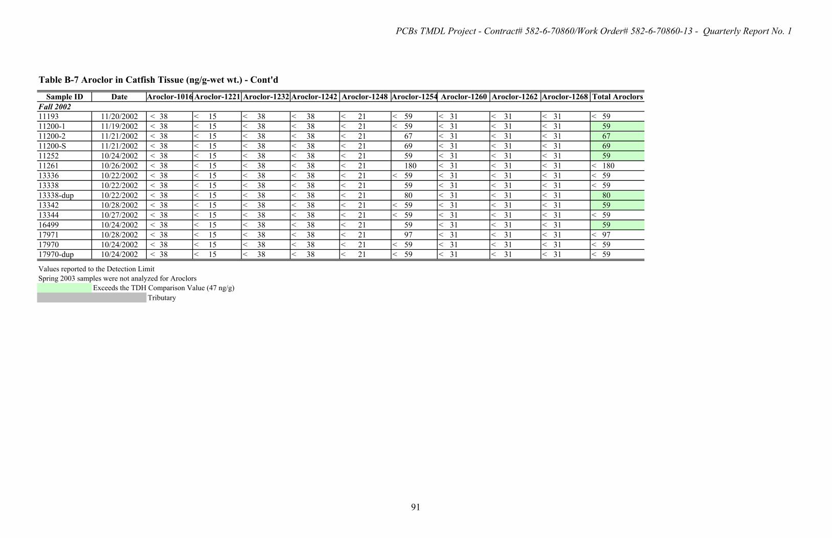
PCBs TMDL Project - Contract# 582-6-70860/Work Order# 582-6-70860-13 - Quarterly Report No. 1
Table B-7 Aroclor in Catfish Tissue (ng/g-wet wt.) - Cont'd
Sample ID Date Aroclor-1016 Aroclor-1221 Aroclor-1232 Aroclor-1242 Aroclor-1248 Aroclor-1254 Aroclor-1260 Aroclor-1262 Aroclor-1268 Total Aroclors Fall 2002 11193 11/20/2002 < 38 < 15 < 38 < 38 < 21 < 59 < 31 < 31 < 31 < 59 11200-1 11/19/2002 < 38 < 15 < 38 < 38 < 21 < 59 < 31 < 31 < 31 59 11200-2 11/21/2002 < 38 < 15 < 38 < 38 < 21 67 < 31 < 31 < 31 67 11200-S 11/21/2002 < 38 < 15 < 38 < 38 < 21 69 < 31 < 31 < 31 69 11252 10/24/2002 < 38 < 15 < 38 < 38 < 21 59 < 31 < 31 < 31 59 11261 10/26/2002 < 38 < 15 < 38 < 38 < 21 180 < 31 < 31 < 31 < 180 13336 10/22/2002 < 38 < 15 < 38 < 38 < 21 < 59 < 31 < 31 < 31 < 59 13338 10/22/2002 < 38 < 15 < 38 < 38 < 21 59 < 31 < 31 < 31 < 59 13338-dup 10/22/2002 < 38 < 15 < 38 < 38 < 21 80 < 31 < 31 < 31 80 13342 10/28/2002 < 38 < 15 < 38 < 38 < 21 < 59 < 31 < 31 < 31 59 13344 10/27/2002 < 38 < 15 < 38 < 38 < 21 < 59 < 31 < 31 < 31 < 59 16499 10/24/2002 < 38 < 15 < 38 < 38 < 21 59 < 31 < 31 < 31 59 17971 10/28/2002 < 38 < 15 < 38 < 38 < 21 97 < 31 < 31 < 31 < 97 17970 10/24/2002 < 38 < 15 < 38 < 38 < 21 < 59 < 31 < 31 < 31 < 59 17970-dup 10/24/2002 < 38 < 15 < 38 < 38 < 21 < 59 < 31 < 31 < 31 < 59
Values reported to the Detection Limit Spring 2003 samples were not analyzed for Aroclors
Exceeds the TDH Comparison Value (47 ng/g) Tributary
91

PCBs TMDL Project - Contract# 582-6-70860/Work Order# 582-6-70860-13 - Quarterly Report No. 1
Table B-8 Aroclors in Crab Tissue (ng/g-wet wt.)
Sample ID Date Aroclor-1016 Aroclor-1221 Aroclor-1232 Aroclor-1242 Aroclor-1248 Aroclor-1254 Aroclor-1260 Aroclor-1262 Aroclor-1268 Total Aroclors Summer 2002 11200 09/02/2002 < 38 < 15 < 38 < 38 < 21 < 59 < 31 < 31 < 31 < 59 11252 08/29/2002 < 38 < 15 < 38 < 38 < 21 < 59 < 31 < 31 < 31 < 59 11252-dup 08/29/2002 < 38 < 15 < 38 < 38 < 21 < 59 < 31 < 31 < 31 < 59 11273 08/28/2002 < 38 < 15 < 38 < 38 < 21 < 59 47 < 31 < 31 < 59 11273-dup 08/28/2002 < 38 < 15 < 38 < 38 < 21 < 59 41 < 31 < 31 < 59 11280 08/28/2002 < 38 < 15 < 38 < 38 < 21 66 < 31 < 31 < 31 < 66 11280-dup 08/28/2002 < 38 < 15 < 38 < 38 < 21 < 59 41 < 31 < 31 < 59 11287 08/25/2002 < 38 < 15 < 38 < 38 < 21 < 59 47 < 31 < 31 < 59 11287 08/25/2002 < 38 < 15 < 38 < 38 < 21 < 59 54 < 31 < 31 < 59 11292 09/11/2002 < 38 < 15 < 38 < 38 < 21 < 59 < 31 < 31 < 31 < 59 11300 09/09/2002 < 38 < 15 < 38 < 38 < 21 < 59 < 31 < 31 < 31 < 59 11302 08/26/2002 < 38 < 15 < 38 < 38 < 21 < 59 < 55 < 31 < 31 59 11382 08/13/2002 < 38 < 15 < 38 < 38 < 21 < 59 < 31 < 31 < 31 < 59 13309 09/11/2002 < 38 < 15 < 38 < 38 < 21 < 59 < 31 < 31 < 31 < 59 13336 08/28/2002 < 38 < 15 < 38 < 38 < 21 < 59 < 31 < 31 < 31 < 59 13338 08/23/2002 < 38 < 15 < 38 < 38 < 21 < 59 < 31 < 31 < 31 < 59 13339 08/25/2002 < 38 < 15 < 38 < 38 < 21 < 59 35 < 31 < 31 59 13339-dup 08/25/2002 < 38 < 15 < 38 < 38 < 21 < 59 31 < 31 < 31 < 59 13341 08/16/2002 < 38 < 15 < 38 < 38 < 21 < 59 < 31 < 31 < 31 < 59 13342 08/24/2002 < 38 < 15 < 38 < 38 < 21 < 59 < 31 < 31 < 31 < 59 13343 09/04/2002 < 38 < 15 < 38 < 38 < 21 < 59 < 31 < 31 < 31 < 59 13344 08/23/2002 < 38 < 15 < 38 < 38 < 21 < 59 36 < 31 < 31 < 59 13344-dup 08/23/2002 < 38 < 15 < 38 < 38 < 21 < 59 61 < 31 < 31 < 61 14560 08/30/2002 < 38 < 15 < 38 < 38 < 21 < 59 < 31 < 31 < 31 < 59 15908 09/11/2002 < 38 < 15 < 38 < 38 < 21 < 59 < 31 < 31 < 31 < 59 15979 09/05/2002 < 38 < 15 < 38 < 38 < 21 < 59 < 31 < 31 < 31 < 59 16213 09/10/2002 < 38 < 15 < 38 < 38 < 21 < 59 < 31 < 31 < 31 < 59 16496 08/24/2002 < 38 < 15 < 38 < 38 < 21 < 59 < 46 < 31 < 31 < 59 16499 08/23/2002 < 38 < 15 < 38 < 38 < 21 < 59 < 31 < 31 < 31 < 59 16618 08/20/2002 < 38 < 15 < 38 < 38 < 21 < 59 < 31 < 31 < 31 < 59 16622 09/02/2002 < 38 < 15 < 38 < 38 < 21 < 59 < 31 < 31 < 31 < 59 17971 08/24/2002 < 38 < 15 < 38 < 38 < 21 < 59 < 50 < 31 < 31 < 59
92

PCBs TMDL Project - Contract# 582-6-70860/Work Order# 582-6-70860-13 - Quarterly Report No. 1
Table B-8 Aroclors in Crab Tissue (ng/g-wet wt.) - Cont'd
Sample ID Date Aroclor-1016 Aroclor-1221 Aroclor-1232 Aroclor-1242 Aroclor-1248 Aroclor-1254 Aroclor-1260 Aroclor-1262 Aroclor-1268 Total Aroclors Fall 2002 11193 10/21/2002 < 38 < 15 < 38 < 38 < 21 < 59 < 31 < 31 < 31 < 59 11252 11/13/2002 < 38 < 15 < 38 < 38 < 21 < 59 < 31 < 31 < 31 < 59 11261 10/25/2002 < 38 < 15 < 38 < 38 < 21 < 59 < 31 < 31 < 31 < 59 13336 10/22/2002 < 38 < 15 < 38 < 38 < 21 < 59 < 31 < 31 < 31 < 59 13338 10/22/2002 < 76 < 30 < 76 < 76 < 42 < 120 < 62 < 62 < 62 < 120 13340 10/22/2002 < 38 < 15 < 38 < 38 < 21 < 59 < 31 < 31 < 31 < 59 16499 10/24/2002 < 38 < 15 < 38 < 38 < 21 < 59 < 31 < 31 < 31 < 59 13342 10/28/2002 < 76 < 30 < 76 < 76 < 42 < 120 < 62 < 62 < 62 < 120 13344 10/27/2002 < 38 < 15 < 38 < 38 < 21 < 59 < 31 < 31 < 31 < 59 13344-dup 11/14/2002 < 38 < 15 < 38 < 38 < 21 < 59 < 31 < 31 < 31 < 59 13363 11/16/2002 < 38 < 15 < 38 < 38 < 21 < 59 < 31 < 31 < 31 < 59 15464 11/13/2002 < 38 < 15 < 38 < 38 < 21 < 59 < 31 < 31 < 31 < 59 17971 10/28/2002 < 38 < 15 < 38 < 38 < 21 < 59 < 31 < 31 < 31 < 59 17971-dup 10/28/2002 < 76 < 30 < 76 < 76 < 42 < 120 < 62 < 62 < 62 < 120 17970 10/24/2002 < 38 < 15 < 38 < 38 < 21 < 59 < 31 < 31 < 31 < 59
Values reported to the Detection Limit Spring 2003 samples were not analyzed for Aroclors
Exceeds the TDH Comparison Value (47 ng/g) tributary
93