Embed Size (px)
Citation preview

Abstract
Quantum phases and transitions of many-body
systems realized using cold atomic gases
Stephen Christopher Powell
2007
In recent years, new advances in techniques for trapping and cooling atoms have
allowed the production of atomic gases at low-enough temperatures and high-enough
densities for collective quantum-mechanical e!ects to become important. This thesis
describes theoretical investigations of certain many-body physics problems motivated
by these experimental developments. It consists of two main parts.
In the first, I investigate the array of phases exhibited by degenerate mixtures
of bosons and fermions with a Feshbach resonance, a bound molecular state whose
energy can be tuned with a magnetic field. These phases are distinguished by the
presence or absence of a bosonic condensate and also by the di!erent Luttinger
constraints that are shown to apply to the Fermi surface(s).
The second part is concerned with bosons in an optical lattice, in which a periodic
potential is produced by counterpropagating lasers. Spinless bosons are known to
exhibit a quantum phase transition between a Mott insulator and a superfluid state,
while bosons with spin have a much richer phase structure. I consider, in particu-
lar, a phase transition with a spinless order parameter, and show that the long-time
dynamics of spin-carrying excitations is governed by a nontrivial fixed point. The
corresponding anomalous exponents are found using a renormalization-group calcu-
lation.
Quantum phases and transitions of
many-body systems realized using cold
atomic gases
A DissertationPresented to the Faculty of the Graduate School
ofYale University
in Candidacy for the Degree ofDoctor of Philosophy
byStephen Christopher Powell
Dissertation Director: Ramamurti Shankar
May 2007

Copyright c! 2007 by Stephen Christopher Powell
All rights reserved.
ii

Contents
1 Introduction 1
1.1 Feshbach resonance . . . . . . . . . . . . . . . . . . . . . . . . . . . . 2
1.2 Optical lattices . . . . . . . . . . . . . . . . . . . . . . . . . . . . . . 5
1.3 Atoms with spin . . . . . . . . . . . . . . . . . . . . . . . . . . . . . . 7
1.4 Outline . . . . . . . . . . . . . . . . . . . . . . . . . . . . . . . . . . . 8
2 Bose-Fermi mixtures 10
2.1 Introduction . . . . . . . . . . . . . . . . . . . . . . . . . . . . . . . . 10
2.2 Basic definitions . . . . . . . . . . . . . . . . . . . . . . . . . . . . . . 12
2.3 The limit g " 0 . . . . . . . . . . . . . . . . . . . . . . . . . . . . . . 15
2.4 Mean-field theory . . . . . . . . . . . . . . . . . . . . . . . . . . . . . 17
2.4.1 Mean-field Hamiltonian . . . . . . . . . . . . . . . . . . . . . . 18
2.4.2 Particle numbers . . . . . . . . . . . . . . . . . . . . . . . . . 19
2.4.3 Zero-temperature phases . . . . . . . . . . . . . . . . . . . . . 22
2.5 Luttinger’s theorem . . . . . . . . . . . . . . . . . . . . . . . . . . . . 29
2.6 Quantum phase transitions . . . . . . . . . . . . . . . . . . . . . . . . 34
2.6.1 Mean-field approximation . . . . . . . . . . . . . . . . . . . . 35
2.6.2 Boson propagator . . . . . . . . . . . . . . . . . . . . . . . . . 36
2.6.3 Critical field theories . . . . . . . . . . . . . . . . . . . . . . . 38
iii

2.7 Gaussian corrections . . . . . . . . . . . . . . . . . . . . . . . . . . . 38
2.7.1 Renormalization of the detuning . . . . . . . . . . . . . . . . . 39
2.7.2 Atom-number corrections . . . . . . . . . . . . . . . . . . . . 41
2.8 Conclusions . . . . . . . . . . . . . . . . . . . . . . . . . . . . . . . . 42
3 Bosons with spin 44
3.1 Introduction . . . . . . . . . . . . . . . . . . . . . . . . . . . . . . . . 44
3.2 Model . . . . . . . . . . . . . . . . . . . . . . . . . . . . . . . . . . . 46
3.2.1 Hamiltonian . . . . . . . . . . . . . . . . . . . . . . . . . . . . 46
3.2.2 Classification of phases . . . . . . . . . . . . . . . . . . . . . . 48
3.2.3 Continuum action . . . . . . . . . . . . . . . . . . . . . . . . . 49
3.3 Mean-field theory . . . . . . . . . . . . . . . . . . . . . . . . . . . . . 50
3.3.1 Strong-pairing limit . . . . . . . . . . . . . . . . . . . . . . . . 51
3.3.2 Quantum rotor operators . . . . . . . . . . . . . . . . . . . . . 51
3.3.3 Mean-field Hamiltonian . . . . . . . . . . . . . . . . . . . . . . 52
3.3.4 Variational wavefunction . . . . . . . . . . . . . . . . . . . . . 54
3.4 Properties of phases . . . . . . . . . . . . . . . . . . . . . . . . . . . . 56
3.4.1 Spin-singlet insulator . . . . . . . . . . . . . . . . . . . . . . . 56
3.4.2 SSI near SSC . . . . . . . . . . . . . . . . . . . . . . . . . . . 58
3.4.3 Spin-singlet condensate . . . . . . . . . . . . . . . . . . . . . . 62
3.5 Critical properties . . . . . . . . . . . . . . . . . . . . . . . . . . . . . 65
3.5.1 Renormalization group . . . . . . . . . . . . . . . . . . . . . . 66
3.5.2 Perturbation theory . . . . . . . . . . . . . . . . . . . . . . . . 72
3.6 Conclusions . . . . . . . . . . . . . . . . . . . . . . . . . . . . . . . . 74
4 Summary and outlook 76
4.1 Bose-Fermi mixtures: recent experiments . . . . . . . . . . . . . . . . 77
iv
4.2 Universality in quantum liquids . . . . . . . . . . . . . . . . . . . . . 78
4.3 Extensions of Luttinger’s theorem in related systems . . . . . . . . . 78
4.4 Assumption of spatial uniformity . . . . . . . . . . . . . . . . . . . . 79
4.5 Excited-state spectra at other pairing transitions . . . . . . . . . . . . 80
4.6 Other transitions of spinful bosons in optical lattices . . . . . . . . . 81
Appendix 82
A.1 Dressed molecular propagator . . . . . . . . . . . . . . . . . . . . . . 82
A.1.1 Diagrammatic description . . . . . . . . . . . . . . . . . . . . 82
A.1.2 Calculations . . . . . . . . . . . . . . . . . . . . . . . . . . . . 83
A.1.3 Spectral representation . . . . . . . . . . . . . . . . . . . . . . 84
A.2 Stability against phase separation . . . . . . . . . . . . . . . . . . . . 87
A.2.1 The compressibility matrix . . . . . . . . . . . . . . . . . . . . 87
A.2.2 Physical interpretation . . . . . . . . . . . . . . . . . . . . . . 89
A.2.3 Results . . . . . . . . . . . . . . . . . . . . . . . . . . . . . . . 90
A.3 Momentum cuto! RG . . . . . . . . . . . . . . . . . . . . . . . . . . 92
A.3.1 Self-energy renormalization . . . . . . . . . . . . . . . . . . . 92
A.3.2 Partition function . . . . . . . . . . . . . . . . . . . . . . . . . 94
A.3.3 Rescaling . . . . . . . . . . . . . . . . . . . . . . . . . . . . . 95
A.3.4 Renormalized propagator . . . . . . . . . . . . . . . . . . . . . 97
v

Acknowledgments
First and foremost, I thank Subir Sachdev, who acted as my research adviser and
coauthored the two articles that this thesis is based upon. I also thank Ramamurti
Shankar, who took over the reins after Subir’s departure. Both provided plenty of
useful advice on matters of research and much else besides.
I am also deeply indebted to the other members of my dissertation committee,
Steve Girvin, Dave DeMille and Jack Harris, whose insightful questioning helped to
clarify several important points.
I am very grateful to Hans Peter Buchler, who was a coauthor of one of the
two articles, and to Krishnendu Sengupta, with whom I discussed many aspects of
the research. I also thank, amongst others, Mara Baraban, Lorentz Bartosch, Lev
Bishop, Jack Challis, Adrian Del Maestro, Tom Jackson, George Mias, and Terri Yu,
for help and encouragement during my time in the Yale physics department.
I acknowledge financial support from the National Science Foundation and the
William C. G. Ortel Fellowship in Physics.
Finally, many thanks to Michael, Judy and Shialing for their unwavering support
throughout.
vi

List of Figures
2.1 Phase boundary with detuning ! and temperature T , for fixed particle
numbers Nf/Nb = 1.11 and equal atomic masses, mf = mb. The
dashed line has vanishing coupling and has been found with a purely
classical analysis. The solid line has dimensionless coupling "2/T0 =
2.0 # 10!2, and has been determined using the mean-field theory of
Section 2.4. For both, the condensed phase is on the left-hand side (for
lower T ) and labeled $b% &= 0, while the phase without a condensate is
labeled $b% = 0. . . . . . . . . . . . . . . . . . . . . . . . . . . . . . . 21
2.2 Phase boundary with fermion number Nf and detuning !, for three
di!erent temperatures. The coupling is "2/T0 = 2.5 # 10!4 and the
atomic masses are equal. The two phases are labeled as in Fig. 2.1,
with the condensed phase favored for higher detuning, lower fermion
number and lower temperature. . . . . . . . . . . . . . . . . . . . . . 22
vii

2.3 The phase diagram at T = 0 with dimensionless couplings (a) "2/T0 =
0, (b) "2/T0 = 2.5 # 10!4 and (c) "2/T0 = 2.0 # 10!2. The at-
omic masses are equal and the coupling between bosons is given by
#2(mb)3T0 = 2 # 10!3. The three distinct phases have, respectively,
no Bose-Einstein condensate and two Fermi surfaces (labeled ‘2 FS,
no BEC’), a condensate and two Fermi surfaces (‘2 FS + BEC’), and
a condensate and a single Fermi surface (‘1 FS + BEC’). The dotted
line indicates the fermion number at which Fig. 2.4 is plotted. . . . . 24
2.4 The e!ective mass m! at the Fermi surface, with fermion number
Nf = 0.1Nb, coupling "2/T0 = 2.5 # 10!4, and equal atomic masses.
As can be seen from the dotted line in Fig. 2.3, these parameters give
a phase with a single Fermi surface. This surface changes from having
a molecular character, with m! ' m", to having an atomic character,
m! ' mf . . . . . . . . . . . . . . . . . . . . . . . . . . . . . . . . . . 25
2.5 The Fermi wavenumbers for the two mixed species of fermions, " and
F , with coupling "2/T0 = 2.5 # 10!4 and equal atomic masses. The
solid lines have fermion number Nf = 32Nb, while the dashed lines have
Nf = 12Nb. As can be seen in Fig. 2.3, the solid line goes between all
three phases (at !/T0 ' 0.25 and !/T0 ' 2.9), while the dashed line
goes from the phase with a single Fermi surface to that having two
and back again (at !/T0 ' (0.65 and !/T0 ' 1.3). The wavenumbers
are measured in units of kf0 , the Fermi wavenumber for free fermions
with number Nf . . . . . . . . . . . . . . . . . . . . . . . . . . . . . . 26
viii

2.6 The phase diagram in the grand canonical ensemble, with the fermion
chemical potential µf plotted on the vertical axis and the detuning !
on the horizontal axis. The number ratio Nf/Nb is allowed to vary in
this plot. The boundary between ‘2 FS, no BEC’ and ‘1 FS + BEC’
in Fig. 2.3 expands into a new phase, labeled ‘1 FS, no BEC’, within
which there are only molecules, whose density is constant (both Nf
and Nb remain fixed in this phase). The atomic masses are equal, and
the couplings are "2/T0 = 2.5 # 10!4 and #2(mb)3T0 = 2 # 10!3. . . . 28
2.7 Two-loop corrections to the atom numbers, shown as a fraction of the
total numbers evaluated to lowest order, and plotted as a function of
the dimensionless coupling "2/T0. The detuning is fixed at !/T0 = 0.5,
the atomic masses are equal, mf = mb, and the temperature is zero.
At each value of the coupling, the parameters have been chosen to put
the system just inside the ‘2 FS, no BEC’ phase. . . . . . . . . . . . . 42
3.1 Phase diagram for the Hamiltonian in Eq. (3.1) calculated using the
mean-field theory of Section 3.3. The three phases that are included
are the spin-singlet insulator (SSI), the spin-singlet condensate (SSC),
and the polar condensate (PC). The calculation has been performed
using quantum rotors, corresponding to the canonical ensemble with
the filling factor an even integer. The horizontal and vertical axes give
the hopping strength t and the spin-dependent part of the interaction
J , both in units of the spin-independent part of the interaction, U . . 55
ix

3.2 The spectral weight $" in SSI, calculated up to second order in the
couplings u and v. The delta-function peak at % = # (which has
artificially been given a small but nonzero width) describes the stable
particle excitation of the field &µ. For % > 3#, there is continuum of
three-particle excitations. . . . . . . . . . . . . . . . . . . . . . . . . . 59
3.3 The spectral weight $" in SSI near the transition to SSC, calculated
up to order g2", plotted for three di!erent values of #!, the gap to
pair excitations. The coupling strength is g" = 0.1. The peak at
% = # (which is present for all values of #! and has artificially been
given a small but nonzero width) describes the stable particle and
hole excitation of the field &µ. For % > #+ #!, there is continuum of
excitations, corresponding physically to the conversion of a particle to
a pair plus a hole. . . . . . . . . . . . . . . . . . . . . . . . . . . . . . 61
3.4 The spectral weight $# for the field 'Iµ in SSC, near the gap #I , calcu-
lated numerically using the diagram in Eq. (3.32). As in Figs. 3.2 and
3.3, there is a delta-function peak at % = #I (which has artificially
been given a nonzero width), corresponding to the stable particle ex-
citation. In this case, unlike in SSI, the continuum in the spectral
weight occurs immediately above the peak. This is due to the (gap-
less) Goldstone mode ( resulting from the broken phase symmetry in
SSC. The derivatives in the coupling between the Goldstone mode and
the 'Iµ field in SSSC strongly suppress the spectral weight as % " #I
from above; in fact, $# ) (% ( #I)3. . . . . . . . . . . . . . . . . . . . 64
x

3.5 The spectral weight $" at the SSI–SSC transition in d = 2 spatial
dimensions. The delta-function peak at % = # has been replaced by a
continuum of excitations, with $" ) (%(#)!1+$! . The numerical value
)" = 0.91797 used in the plot results from a dimensional expansion in
* = 3 ( d, carried out to order *2, Eq. (3.51), and evaluated at * = 1. 70
3.6 The spectral weight $" at the SSI–SSC transition in d = 3 spatial
dimensions. The delta-function peak at % = # has been replaced by a
continuum of excitations, with the mean-field exponent $" ) (%( #)!1. 73
A.1 The spectral weight $"0 of the molecule in vacuum for a narrow Fesh-
bach resonance, with "2/T0 = 2.5#10!4, for three di!erent detunings.
(The density is zero in this plot, so T0 is an arbitrarily chosen unit
of energy.) The curves have all been evaluated at zero momentum; a
nonzero momentum k would simply shift the curves to the right by
an amount k2/(2m"). For ! < 0, there is a delta-function peak for
negative x, which has artificially been given a finite width. For all !,
there is a continuum for x > 0, but this is too small to be visible for
!/T0 = (1. . . . . . . . . . . . . . . . . . . . . . . . . . . . . . . . . 85
A.2 As Fig. A.1, but for a broader resonance, "2/T0 = 0.1. . . . . . . . . . 86
A.3 The phase diagram at T = 0, as in Fig. 2.3, with couplings "2/T0 =
2.0# 10!2 and #2(mb)3T0 = 2# 10!3. The other parameters, and the
labels for the three phases, are the same as in Fig. 2.3. The region
where the phase is unstable, as determined in Section A.2, is indicated. 91
xi

Chapter 1
Introduction
The behavior of physical systems with many constituent parts interacting strongly
with each other has long been a central concern in the theory of condensed matter.
It is only within roughly the past decade that it has been possible to produce gases of
atoms at su#ciently high density and low temperature that the e!ects of their mutual
interactions become significant. These systems, while interesting in their own right,
also provide a useful toolbox for the study of many-body physics in other contexts.
This thesis will describe theoretical studies of two examples of such systems.
The recent growth of interest in many-body phenomena in atomic systems was
started by the realization, in 1995, of a Bose-Einstein condensate (BEC) in an ‘ultra-
cold’ gas of rubidium atoms [1]. Bose-Einstein condensation, predicted in 1924 [2–4],
refers to the macroscopic occupation of a single quantum state [5, 6]. It was recog-
nized as the cause of superfluidity in liquid helium as early as 1938 [7,8], but strong
interactions in that system made quantitative comparisons with theory di#cult [9].
There are several attractive features of ultracold atomic gases that have caused
them to be the focus of particular interest. An immediate advantage of the atomic
BEC was that the relatively weak interactions allowed for more direct comparison
1

CHAPTER 1. INTRODUCTION 2
with the theory of weakly interacting bosons [10, 11].
A second advantage is the ability to observe condensation directly by probing
the momentum-space distribution of the atoms. In a typical experiment, the atoms
are trapped within a tight optical or magnetic potential [12, 13], and then suddenly
released, by rapidly switching o! the potential [1]. Using the ‘sudden approxima-
tion’ [14], the atoms are projected onto momentum states, and subsequently evolve
essentially independently [15]. After a certain ‘time of flight’ has elapsed, the spatial
density profile of the cloud is measured (for example, via the optical density for ab-
sorption) which, assuming free propagation after the trap is released, gives a direct
measurement of the momentum-space distribution prior to release. Bose-Einstein
condensation is then signaled by the appearance of a sharp peak near zero momen-
tum, superimposed upon the thermal distribution [1]. It is also possible to measure
correlations in the momentum distribution, as a means to identify quantum states
with nontrivial correlations [15].
A third advantage, the extent to which their properties can be controlled and
modified in experiments, has led to the development of a vast array of new experi-
mental techniques, motivated, in large part, by the goal of simulating various systems
of interest in solid-state physics [16–19]. In the remainder of this chapter, I will give
a brief description of some of these techniques and the theoretical models that have
been used to describe them.
1.1 Feshbach resonance
The Feshbach resonance [20–22], which originated in nuclear physics and was first
demonstrated in an atomic context by Inouye et al. [23], has emerged as a useful
technique for forming bound states of neutral atoms. The term refers to a molecular
CHAPTER 1. INTRODUCTION 3
state whose binding energy can be ‘tuned’ by varying an external parameter. For
example, by choosing a bound state with a di!erent magnetic moment from the
unbound atoms, the relative energy of the resonance can be changed with an external
magnetic field [23, 24].
A simple model Hamiltonian can be written as [25]
H =
!ddx
"#
%"{1,2}
&†%
$(
*2
2m%( µ%
%&% +"†
&(
*2
2(m1 + m2)( (µ1 + µ2) + !
'"
+ g("†&1&2 + &†
2&†1")*
, (1.1)
where &% is the field (annihilation) operator for atomic species1 +, m% and µ% are
the corresponding mass and chemical potential, and " is the field operator for the
molecular state. The energy of the bound state relative to the two-atom continuum
is denoted ! and referred to as the detuning.
The final term in H represents the physical process where two atoms combine to
form a molecule, as well as its opposite. Interactions other than this pairing term
are assumed to be less important near resonance and have been omitted.
One e!ect of the Feshbach resonance is to alter the scattering properties for the
atomic species. For ! + 0, the scattering length a between the two atoms is domi-
nated by the presence of the bound state " [26]. Su#ciently close to the resonance,
a is inversely proportional to ! [22], so that the strength of the interaction can be
adjusted over a wide range of values, both attractive and repulsive. The enhanced
scattering near resonance can be viewed as resulting from virtual transitions into the
molecular state.
The presence of the molecular state also allows for new and interesting many-
1For bosonic atoms, the two atoms may be of the same species, in which case the index ! shouldbe ignored throughout.

CHAPTER 1. INTRODUCTION 4
body phases, with various possibilities depending on the quantum statistics of the
atomic species.
If both atoms are fermions, the molecular species " is a boson, and a BEC of
molecules is formed at low temperature [27–29], provided ! is not too large. For
! , 0, where formation of molecules is unfavorable, the system crosses over into
a state of paired fermions [30], analogous to the BCS phenomenon in metals [31].
The ‘BCS–BEC crossover’ between these regimes has been the subject of particular
interest, both experimental [32,33] and theoretical [34,35]. (For a recent review, see
Ref. [36].)
The case of a Feshbach resonance between two atoms of the same species of bosons
has also been considered [37,38]. In this case, a BEC of individual atoms is possible
for ! , 0, while a BEC of molecules again forms for ! - 0. Unlike the fermionic
case, these two states cannot be connected smoothly to each other2 and a quantum
phase transition between the two occurs at some value of ! [37, 38].
The third possibility, a Feshbach resonance between a fermion and a boson, has
been observed experimentally by several groups [39–41]. Chapter 2 will consider this
case in some detail, and show that various phases are possible, distinguished by the
presence or absence of an atomic BEC, and the number of Fermi surfaces. Observing
these phases in experiment requires simultaneous degeneracy of both atomic species
[42, 43] and of the molecule. In Section 4.1, we describe some recent experimental
developments in this direction.
A purely optical Feshbach resonance has also been predicted [44] and observed
[45]. This allows rotation symmetry to be preserved and hence the manipulation of
2This can mostly easily be seen by considering the symmetries that are broken in the two cases.There is a U(1) symmetry operation of H under which " " "ei! and ! " !e2i!, corresponding tothe conservation of the total number of atoms. A BEC of atoms, $"% &= 0, breaks this symmetrycompletely, whereas with only a BEC of molecules, $!% &= 0, the special case of # = $ remains asan unbroken Z2 symmetry. This distinguishes the two cases qualitatively and shows that they mustbe divided by a phase transition at which the Z2 symmetry is broken [37, 38].

CHAPTER 1. INTRODUCTION 5
multiple spin species, as described below in Section 1.3.
1.2 Optical lattices
A parallel experimental advance, of great significance from the point of view of
simulation of solid-state systems, has been the development of optical lattices [46–49].
Laser trapping uses the e!ective potential produced by the AC Stark e!ect [50]
to confine atoms, which are attracted to maxima or minima of the intensity (with
red- or blue-detuned light, respectively). By using a pair of counterpropagating
laser beams, it is possible to set up a standing light wave; using three such pairs, a
three-dimensional periodic lattice potential can be produced.
This allows for unprecedented control over the parameters of the lattice: the depth
of the potential is determined by the intensity of the light and the lattice constant by
its wavelength. By making the intensity in the three directions highly anisotropic, the
lattice can be made e!ectively one- or two-dimensional. Besides simple square and
cubic lattices, it is possible to produce more complicated structures by appropriate
choice of the relative phases and directions of the lasers. (See, for instance, Ref. [51],
which gives a prescription for producing a Kagome lattice.)
The single-particle states of atoms in an optical lattice potential, like those of
electrons in a crystal, can be divided into bands, with each state assigned a crystal
momentum by Bloch’s theorem. At the low temperatures achievable in experiments,
only the lowest band is populated, and it is more convenient to choose a basis for
the states within this band that is maximally localized in position space. There is
then one such Wannier state [52, 53] for each minimum of the periodic potential.
An e!ective Hamiltonian can then be written in this basis, and a simple and
important example is the Hubbard model [54], originally used to describe electrons

CHAPTER 1. INTRODUCTION 6
in a solid. In the case of spinless bosons [19, 48], it is often referred to as the Bose-
Hubbard model and the Hamiltonian can be written
H = (t#
#ij$
a†iaj +
U
2
#
i
ni(ni ( 1) . (1.2)
Here, ai is the annihilation operator for a boson in the Wannier state localized at site
i of the lattice, and ni = a†iai is the corresponding number operator. The first term
allows for tunneling (‘hopping’) between adjacent sites: the notation $ij% denotes
a sum over nearest-neighbor pairs of sites. The second term represents the mutual
interaction of the atoms, and has been written to give a potential-energy ‘cost’ of U
for every pair of atoms on the same site.3
The phase structure of the Bose-Hubbard model can be understood by considering
separately the two limits t/U " 0 and t/U " . [55, 56]. We assume that there is
a fixed total number of atoms and that this is chosen so that the average number of
atoms per site is an integer.
For t = 0, the model consists of a set of unconnected sites and the atoms will ar-
range themselves uniformly throughout the lattice, in order to minimize their mutual
repulsion and hence the potential energy. This leads to an incompressible state, re-
ferred to as a Mott insulator. For a small nonzero t, virtual tunneling events will lead
to fluctuations in the number on each site, but the system remains an incompressible
insulator for a finite range of t/U .
In the opposite limit, where U = 0, there are no interactions between the particles
and the bosons will condense into the single-particle state with the lowest energy.
The system becomes a superfluid and remains so in the presence of a small finite U ,
but for su#ciently large U/t undergoes a transition into a Mott insulator. A simple
3Note that this simplification, which involves ignoring three-body and higher terms, is not nec-essary for the qualitative analysis, or the mean-field theory described below.

CHAPTER 1. INTRODUCTION 7
mean-field analysis was used in Ref. [55] to connect the two extremes and map out
the phase diagram.
The superfluid–insulator phase transition was first demonstrated using cold at-
omic gases in the work of Greiner et al. [49], which used rubidium-87 atoms in an
optical lattice. Superfluidity of (pairs of) fermions in an optical lattice has also been
reported in Ref. [57].
1.3 Atoms with spin
Another common feature of condensed-matter systems, and one that leads to a great
deal of interesting phenomena, is the presence of spin. While most of the species used
in experiments with ultracold atoms have several hyperfine (nuclear spin) states, it
required the development of purely optical trapping techniques [58] to liberate this
degree of freedom.
For bosonic atoms, where the ground state (in the absence of a lattice) is a
BEC, the condensate wavefunction has the possibility for interesting structure in
spin space [59, 60], with the number of possible phases increasing with the atomic
spin [61]. The actual ground state that is realized depends on the scattering lengths
in the channels with di!erent total spin.
The collective modes above each of these ground states and the response to an
applied magnetic field can be determined using a semiclassical analysis of the dy-
namics of the condensate wavefunction. Also of interest is the dynamics of these
systems when driven far from equilibrium. An example is the so-called ‘spin-mixing’
dynamics [62, 63], which describes the evolution of the occupation numbers of the
di!erent spin components when the system is initially far from its ground state.
In the presence of an optical lattice potential, there are, besides these condensed

CHAPTER 1. INTRODUCTION 8
phases, various possible insulating phases with di!erent types of spin order [64–68].
The phase diagram is particularly rich when the filling factor (the ratio of the number
of bosons to the number of sites in the lattice) is an even integer, in which case both
superfluids and insulators, with and without spin ordering, are possible. Chapter 3
will consider this case and focus on the transition from an insulator to a superfluid
in the absence of spin ordering.
1.4 Outline
This thesis is divided into two main parts, which address two examples of systems
that may be realized using ultracold atomic gases.
Chapter 2: Bose-Fermi mixtures
This chapter is based on Ref. [69]. It is concerned with a mixture of bosonic and
fermionic atoms coupled by a Feshbach resonance to a molecular state. The various
phases of the mixture, assuming simultaneous degeneracy of all three species, are
described. By varying the detuning, temperature and relative numbers of bosons
and fermions, several di!erent phases are found to be possible. We show that, at
zero temperature, the phases can be distinguished by distinct Luttinger constraints
that depend on the presence or absence of a Bose-Einstein condensate and also on
the number of Fermi surfaces.
Chapter 3: Bosons with spin
This chapter, based in part on Ref. [70], describes a system of bosons with spin that
are trapped within an optical lattice. We describe a mean-field theory that allows for
the possibility of a paired condensate that does not break spin symmetry. We consider

CHAPTER 1. INTRODUCTION 9
the behavior of the Green function corresponding to single-particle excitations in the
insulator and the paired superfluid and then show that, at the transition between
the two, the coherent quasiparticles are replaced by an incoherent continuum with a
nontrivial scaling exponent.
Chapter 4: Summary
This chapter summarizes the main results of this thesis and describes related ongoing
and potential future work.
Chapter 2
Bose-Fermi mixtures
2.1 Introduction
In this chapter, we will consider a mixture of bosonic and fermionic atoms with
a Feshbach resonance coupling the pair to a molecular state. Such a system is
analogous those described in Section 1.1, with Feshbach resonances between a pair
of fermions [30, 34–36] and a pair of bosons [37, 38].
In this case, the Feshbach resonance is a bound molecular state consisting of one
bosonic and one fermionic atom, and hence is itself a fermion. The energy of the
resonance can be tuned using an applied magnetic field, as described in Section 1.1,
and the energy di!erence between the bound state and the lower end of the two-atom
continuum will be referred to as the detuning !.
Our primary result is that the mixture displays a variety of phases, distinguished
by the number of Fermi surfaces and the presence or absence of a Bose-Einstein
condensate (BEC). We will use mean-field theory to map out the phase diagram
in terms of !, the temperature T , and the densities of the two types of atom (see
Figs. 2.1, 2.2, 2.3 and 2.6).
10

CHAPTER 2. BOSE-FERMI MIXTURES 11
The existence of a quantum phase transition at zero temperature can be easily
understood by considering the two limiting cases. For ! , 0, molecules are strongly
disfavored, leaving a BEC of the bosonic atoms and a Fermi surface of the fermionic
atoms. In contrast, for ! - 0, a Fermi surface of molecules will be formed. If the
number of fermionic (Nf ) and bosonic (Nb) atoms are unequal, there will also be
some residual atoms which are not in molecules, and these form their own ground
state. For Nf > Nb, the extra fermions will form a separate Fermi surface of atoms,
while for Nb > Nf , the extra bosons will form an atomic BEC.
Note that for Nf > Nb, changing the detuning takes the system between limits
with and without an atomic BEC. There must therefore be a critical detuning at
which the atomic BEC is completely depleted, and all the bosonic atoms have been
absorbed into molecules.
The number of Fermi surfaces also changes as the detuning is varied, and we will
show in Section 2.5 that the statement of Luttinger’s theorem is di!erent in each
phase. In the absence of a BEC, there are generically two Fermi surfaces, one atomic
and one molecular, and their volumes are separately constrained. In the presence
of a BEC, there may be either one or two Fermi surfaces, but there is only a single
Luttinger constraint. In the phase with two Fermi surfaces and a BEC, the total
volume of the Fermi surfaces is fixed by the number of fermionic atoms.
We now give an outline of the contents of the rest of this chapter. First, in
Section 2.2, we define the model Hamiltonian that will be used throughout. In
Section 2.3, we consider the limit of vanishing coupling, which was also described by
the earlier work of Yabu et al. [71]. In this limit, the properties of the mixture are
described by purely thermodynamic considerations and these can be used to map
out the phase diagram.
Section 2.4 finds the phase structure for finite coupling, treating quantum e!ects

CHAPTER 2. BOSE-FERMI MIXTURES 12
using a mean-field approach. In Section 2.5, we describe our results regarding Lut-
tinger’s theorem for the system. In Section 2.6, the mean-field result of Section 2.4 is
reproduced using a field-theoretical approach, which further allows us to characterize
the critical properties of the transition.
In Section 2.7, we estimate the corrections to, and region of validity of, mean-field
theory. Finally, in the appendix, we address the physics of an isolated molecule, and
then consider the stability of the system against separation into two regions with
di!erent densities.
2.2 Basic definitions
The system consists of bosonic atoms b and fermionic atoms f which combine to
form fermionic molecules &. The energy, relative to the chemical potential µ, is for
the atoms
,fk
= *fk( µf =
k2
2mf( µf (2.1)
,bk = *bk ( µb =
k2
2mb( µb (2.2)
and for the molecule
,"k
= *"k( µ" =
k2
2m"( µ" + ! , (2.3)
including the detuning !. The masses obey m" = mf + mb and, because of the
interaction, the chemical potentials are related by µ" = µf + µb.
The grand-canonical Hamiltonian is, in momentum space,
H =
!d3k
(2-)3(,f
kf †kfk + ,b
kb†kbk + ,"
k&†
k&k) + Hint , (2.4)
where fk, bk and &k are annihilation operators for the three species, at momentum k.
CHAPTER 2. BOSE-FERMI MIXTURES 13
We assume that the fermions’ spins are polarized along the direction of the applied
magnetic field, so that both f and & can be treated as spinless. The interaction term
Hint is given by
Hint = ( g
!
k,k!
(&†k+k!fkbk! + b†
k!f†k&k+k!) + #
!
k,k!,k!
b†k+k!b
†k!!k!bk! bk , (2.5)
where+k
denotes+
d3k /(2-)3. (We will consider the case of three spatial dimensions
throughout, but the results can be generalized straightforwardly.)
The first term in Hint allows the bosonic and fermionic atoms to couple and
form molecules, while the second is an interaction between pairs of bosons. We
omit quartic interactions for the fermions because the exclusion principle forbids s-
wave scattering between identical fermions, and we assume that the other allowed
interactions will be less important than the coupling g near resonance.
Taking the dimensions of momentum and energy to be unity, [k] = [E] = 1,
we have [&] = (32 and the same for the operators b and f . (Throughout, we shall
measure temperature, energy and frequency in the same units, so that ! = kB = 1.)
The coupling constants have dimensions [g] = (12 and [#] = (2.
At temperature T = 1/. &= 0, we have six dimensionless parameters. First let
Nb be the total density of bosonic atoms, including those bound in molecules, and
let Nf be the same for fermionic atoms. (We consider a unit volume, so that density
is synonymous with number.) In the absence of any fermions, the bosons would
condense at a temperature [5, 6]
T0 =2-
mb
&Nb
/(32)
' 23
. (2.6)
We can take as dimensionless parameters T/T0 = .0/., Nf/Nb, mf/mb, !/T0, "2/T0

CHAPTER 2. BOSE-FERMI MIXTURES 14
and #2(mb)3T0, where
" =g2
8-
$2mfmb
m"
%3/2
. (2.7)
In what follows, it will not usually be necessary to take account of the coupling
between bosons given by the final term of Hint. Except within the condensed phase,
the main e!ect of # is a renormalization of the boson mass, which can be incorporated
into a redefinition of mb.
Physical units
In order to relate these parameters to experimental values, we may choose a unit of
volume of 10!15 cm3, which gives the unit of momentum as roughly 10!27 kg · m/s.
Taking the unit of mass to be 6 amu, corresponding to a lithium-6 atom, the unit of
energy is roughly 7 # 10!10 eV or 8 µK.
To estimate the parameters of the Feshbach resonance, we use the expression [24]
g =
,2-abg $B$µ
m, (2.8)
where abg is the background scattering length, $B is the width of the resonance and
$µ is the di!erence in magnetic moments. Using the observed background scattering
length between lithium-6 and -7 of abg = 2.0 nm [43], we may estimate the coupling
constant. Taking, for instance $B = 1 G, $µ = µB, the Bohr magneton, we find
g ' 1 in our units. For a boson density Nb = 1015 cm!3 and mass mb = mf = 6 amu,
the value g = 1 gives a dimensionless coupling of "2/T0 = 5 # 10!4.
While the width of the resonance used here, $B = 1 G, is su#ciently large that
$µ$B ! T0, it is nonetheless somewhat smaller than typical experimental values.
For our purposes, a more relevant measure of the resonance ‘width’ is the lifetime
of the molecule state in the vacuum (for ! > 0). This is calculated in Section A.1

CHAPTER 2. BOSE-FERMI MIXTURES 15
of the appendix, where we show that it is determined by the constant ". Since the
relevant energies are on the order of T0, the condition for a narrow resonance is
that "2/T0 - 1. For the numerical results throughout this paper, we will always
remain in this narrow limit, which is analytically more accessible. As noted above, we
expect our results to be at least qualitatively applicable even for the wider Feshbach
resonances observed experimentally.
Following Ref. [38], we take
# =2-
mbabb , (2.9)
where for abb, the scattering length for the boson–boson interaction, we use abb =
0.27 nm [43], giving
#2(mb)3T0 = 2 # 10!3 . (2.10)
The detuning ! appearing in the molecular dispersion relation, Eq. (2.3), is given
by [24]
! = $µ(B ( B0) , (2.11)
where B0 is the magnetic field at resonance and B is the applied field.
2.3 The limit g " 0
The case of vanishing coupling, which can be addressed with a classical approach, has
been considered by Yabu et al. [71]. (The results presented in this section produce
Fig. 3 of Ref. [71], which corresponds to our Fig. 2.3, below.)
For simplicity, we restrict the analysis to zero temperature, but similar arguments
can be made for nonzero temperatures. We call the two Fermi energies *f0 and *"0 ,
and the corresponding wavenumbers kf0 and k"
0 . At zero temperature, all bosons are
at *b = 0 and fermionic atoms or molecules must be added at their respective Fermi

CHAPTER 2. BOSE-FERMI MIXTURES 16
levels.1
The atomic Fermi surface (FS) vanishes when all the fermionic atoms are con-
tained in molecules, so that
k"0 = (6-2 Nf)
1/3 . (2.12)
(The number of states within a unit sphere in momentum space is 1/6-2.) For
this arrangement to be favorable energetically, the molecular Fermi energy, *"0 , must
remain below the lowest atomic energy level. The boundary of the phase without an
atomic FS is therefore where
1
2m"(Nf)
2/3 +!
(6-2)2/3= 0 . (2.13)
Similarly, the molecular FS vanishes at the point when
1
2mf(Nf )
2/3 (!
(6-2)2/3= 0 . (2.14)
The atomic (molecular) FS is therefore only absent for negative (positive) detuning
!.
To find the boundary of the phase with a BEC, we must consider the depletion
of the condensate. Bosons will take fermions and form molecules as long as their
final energy is lower, ie *"0 < *f0 + 0. The phase boundary is therefore where *f0 = *"0 ,
which gives
1
2mf(Nf ( Nb)
2/3 (1
2m"(Nb)
2/3 =!
(6-2)2/3, (2.15)
where the wavenumbers have been determined from Nb and Nf , using the fact that
1Here and throughout this chapter, we make the important assumption that there is no ‘Pauliblocking’ between fermionic atoms and molecules. This implies, for instance, that a fermionic atomand a molecule can simultaneously occupy states with the same momentum. The assumption isjustified provided that the molecule is su"ciently tightly bound that its wavefunction has negligibleoverlap with the low-momentum atomic plane-wave states of interest.

CHAPTER 2. BOSE-FERMI MIXTURES 17
there is no condensate.
The resulting phase diagrams are shown as the dashed lines in Figs. 2.1 and 2.3,
below. It should be noted that, in this limit, the coupling to fermionic atoms reduces
the tendency of the bosons to condense. (The same is true at nonzero temperature.)
2.4 Mean-field theory
It is possible to go beyond the classical analysis used for vanishing coupling, by using
mean-field theory. We will present here two parallel developments, in this section
and Section 2.6. The first is based on single-particle quantum mechanics, using the
mixing between the fermionic dispersion relations caused by the presence of a BEC.
The second uses a field-theoretic approach and considers perturbative corrections to
the bosonic propagator. The former has the advantage of giving a somewhat clearer
physical picture, while the latter leads naturally to higher-order corrections.
In the remainder of this section, we present the quantum-mechanical approach,
starting from the Hamiltonian in Eq. (2.4). First, in Section 2.4.1, we make a mean-
field approximation and diagonalize the new Hamiltonian. We then find the condition
that a BEC should be energetically favorable, within this approximation. Since the
Hamiltonian is defined in the grand canonical ensemble, we must then relate the
chemical potentials to the particle numbers, in Section 2.4.2.
In Section 2.4.3, we restrict our attention to the case of zero temperature, where
transitions occur between states with di!erent numbers of Fermi surfaces. We iden-
tify the positions of these transitions and present the full phase diagram for T = 0.

CHAPTER 2. BOSE-FERMI MIXTURES 18
2.4.1 Mean-field Hamiltonian
To derive a mean-field theory, we make the Bogoliubov approximation [72], replacing
the boson field bk in Eq. (2.4) by a real constant '. The mean-field Hamiltonian is
then
Hmf =
!d3k
(2-)3
-,fkf †kfk + ,"
k&†
k&k ( g'(&†
kfk + f †
k&k)
.( µb'2 + #'4 , (2.16)
which can be diagonalized to
Hmf =
!d3k
(2-)3
(,Fk F †
kFk + ,!k "†
k"k
)( µb'2 + #'4 . (2.17)
The dispersion relations for the mixed fermions F , " are
,F,!k
=1
2
(,fk
+ ,"k
)±
1
2
,(,fk( ,"
k
)2+ 4g2'2 , (2.18)
with the choice that ,Fk/ ,!
kfor all k.
Since mixing causes the dispersion relations to separate, the total energy of the
fermions is lowered by nonzero '. This quantum-mechanical e!ect, in contrast to the
purely classical e!ect described in Section 2.3, therefore acts to favor condensation.
We must analyze the energetics to determine the point at which a condensate
becomes favorable. The grand free energy % is minimized at temperature 1/. by
a Fermi-Dirac distribution of each of the fermionic species F and ". Ignoring the
thermal distribution of bosons, which does not depend on ', the total free energy is
%(') = (µb'2 + #'4 + RF (') + R!(') , (2.19)

CHAPTER 2. BOSE-FERMI MIXTURES 19
where
Rx(') = (1
.
!d3k
(2-)3log/1 + e!&'x
k
0. (2.20)
The phase transition to a state with nonzero ' occurs when the quadratic coef-
ficient changes sign, ie, when
$ 01
2
d2%
d'2
1111#=0
= 0 . (2.21)
Specifically, for negative $, nonzero ' is energetically favored, causing the bosons to
condense. Using Eqs. (2.18), (2.19), and (2.20), we find
$ = (µb + g2
!d3k
(2-)3
nF(,fk) ( nF(,"
k)
,fk( ,"
k
, (2.22)
where nF is the Fermi-Dirac distribution function. The integral equation $ = 0 can
be solved numerically.
2.4.2 Particle numbers
Since experiments are necessarily performed at fixed particle number, the expressions
for the numbers in terms of the chemical potentials must be found. Particles of the
species b, f and & are not independently conserved, so the relevant quantities are Nf
and Nb, the total numbers of fermionic and bosonic atoms, respectively (including
those contained in molecules).
Within our mean-field theory, we must consider the mixed fermionic species F
and ". Since each contains one atomic fermion, we have
Nf =
!d3k
(2-)3
2nF(,!k ) + nF(,F
k )3
. (2.23)

CHAPTER 2. BOSE-FERMI MIXTURES 20
The number of bosons is (with nB the Bose-Einstein distribution function)
Nb = '2 +
!d3k
(2-)3
2nB(,b
k) + nF(,!k ) cos2 (k + nF(,Fk ) sin2 (k
3, (2.24)
where the first term represents the condensate, the first term in the integrand is the
thermal distribution of the bosons, and (k is the mixing angle.2
When ' = 0, such as along the boundary to the phase without a BEC, the
expression for the number of bosons simplifies to
Nb =
!d3k
(2-)3
-nB(,b
k) + nF(,"k).
. (2.25)
To locate this phase boundary for fixed particle numbers, we must find the values
of µf and µb which give the required numbers and also satisfy $ = 0. (Of course, a
third parameter must be tuned to its critical value to satisfy these three conditions
simultaneously.)
Results from such a procedure are displayed in Fig. 2.1, which shows the boundary
for Nf/Nb = 1.11 as a function of the detuning ! and temperature T = 1/.. The
masses of the atoms are equal, mf = mb, and the solid line has dimensionless coupling
"2/T0 = 2.5 # 10!4. For comparison, the case of vanishing coupling, treated in
Section 2.3, is also shown, with a dashed line. Both curves tend to T = T0, as in the
case of free bosons, when ! " . so that molecules cannot be formed.
In Fig. 2.2, the same phase boundary is shown on a graph of fermion number
versus detuning, for three di!erent temperature values. The solid line is at zero
temperature, T = 0, while the two dashed lines have nonzero temperatures. The
coupling is "2/T0 = 2.5 # 10!4 and the masses are equal, mf = mb. As expected,
2Explicitly, #k is the angle parametrizing the unitary transformation from the fermions f and "in Eq. (2.16) to the fermions F and ! in Eq. (2.17).

CHAPTER 2. BOSE-FERMI MIXTURES 21
$b% &= 0
$b% = 0
Temperature T/T0
Det
unin
g!/T
0
10.80.60.40.20
8
6
4
2
0
(2
Figure 2.1: Phase boundary with detuning ! and temperature T , for fixed particlenumbers Nf/Nb = 1.11 and equal atomic masses, mf = mb. The dashed line hasvanishing coupling and has been found with a purely classical analysis. The solidline has dimensionless coupling "2/T0 = 2.0 # 10!2, and has been determined usingthe mean-field theory of Section 2.4. For both, the condensed phase is on the left-hand side (for lower T ) and labeled $b% &= 0, while the phase without a condensate islabeled $b% = 0.

CHAPTER 2. BOSE-FERMI MIXTURES 22
T/T0 = 0.6T/T0 = 0.3T/T0 = 0
$b% = 0
$b% &= 0
Detuning !/T0
Fer
mio
nnu
mber
Nf/N
b
10.50(0.5(1(1.5(2
1.4
1.2
1
0.8
0.6
Figure 2.2: Phase boundary with fermion number Nf and detuning !, for threedi!erent temperatures. The coupling is "2/T0 = 2.5 # 10!4 and the atomic massesare equal. The two phases are labeled as in Fig. 2.1, with the condensed phasefavored for higher detuning, lower fermion number and lower temperature.
Bose condensation is favored by lower temperatures, as in the case of an isolated
Bose gas.
It remains to be shown that the system is stable against separation into regions
with di!erent densities. This question will be addressed in Section A.2 of the ap-
pendix.
2.4.3 Zero-temperature phases
At T = 0, the Fermi-Dirac distribution function is replaced by a unit step and all
bosons occupy the lowest-energy state. As noted by Yabu et al. [71], the phase
diagram can be further divided into a region with two Fermi surfaces and a region
with a single Fermi surface. (We ignore the trivial case without any Fermi surfaces,
which requires Nf = 0.)
Except when the atomic numbers precisely match, Nf = Nb, the case of a single

CHAPTER 2. BOSE-FERMI MIXTURES 23
Fermi surface can only occur when there is a BEC. In this case, ', the expectation
value of b, is given by the minimum of the free energy % given in Eq. (2.19), so that
we must solve
(2µb '+ 4#'3 +dRF
d'+
dR!
d'= 0 (2.26)
(excluding the root ' = 0).
Following the choice that ,Fk/ ,!
kin Eq. (2.18), the second Fermi surface disap-
pears when ,Fk=0
= 0, making the Fermi wavenumber for F fermions vanish. For this
to be the case, we require µf > 0, µ" > ! and
g' =4
µf(µ" ( !) , (2.27)
which should be solved simultaneously with Eq. (2.26).
These expressions, along with the results in Section 2.4.2 for the particle numbers,
allow the complete zero-temperature phase diagram to be plotted. In Fig. 2.3, the
phase boundaries are shown on a graph of fermion number against detuning, for
equal atomic masses. The three sets of boundaries have couplings (a) "2/T0 = 0, (b)
"2/T0 = 2.5#10!4 and (c) "2/T0 = 2.0#10!2. (Note that the dimensionless coupling
"2/T0 depends on the fourth power of the coupling g appearing in the Hamiltonian,
so a large change in "2/T0 is required for a noticeable change in the phase diagram.
All of these coupling values are within the narrow resonance regime.) Throughout,
we take #2(mb)3T0 = 2 # 10!3; we have verified that, within a reasonable range of
values, changing this parameter has no significant e!ect.
The boundaries divide the diagram into three regions, depending on the presence
of a condensate and the number of Fermi surfaces. In the region labeled ‘2 FS, no
BEC’, the discriminant $ is positive, so there is no BEC and two Fermi surfaces. In
the region labeled ‘2 FS + BEC’, $ is negative and there is a condensate, as well

CHAPTER 2. BOSE-FERMI MIXTURES 24
cb
a 1 FS + BEC
2 FS + BEC
2 FS, no BEC
Detuning !/T0
Fer
mio
nnu
mber
Nf/N
b
3210(1(2
2
1.5
1
0.5
0
Figure 2.3: The phase diagram at T = 0 with dimensionless couplings (a) "2/T0 =0, (b) "2/T0 = 2.5 # 10!4 and (c) "2/T0 = 2.0 # 10!2. The atomic masses areequal and the coupling between bosons is given by #2(mb)3T0 = 2 # 10!3. Thethree distinct phases have, respectively, no Bose-Einstein condensate and two Fermisurfaces (labeled ‘2 FS, no BEC’), a condensate and two Fermi surfaces (‘2 FS +BEC’), and a condensate and a single Fermi surface (‘1 FS + BEC’). The dotted lineindicates the fermion number at which Fig. 2.4 is plotted.

CHAPTER 2. BOSE-FERMI MIXTURES 25
Detuning !/T0
E!ec
tive
mas
sm
!/m
b
3210(1(2(3
2.5
2
1.5
1
0.5
Figure 2.4: The e!ective mass m! at the Fermi surface, with fermion number Nf =0.1Nb, coupling "2/T0 = 2.5 # 10!4, and equal atomic masses. As can be seen fromthe dotted line in Fig. 2.3, these parameters give a phase with a single Fermi surface.This surface changes from having a molecular character, with m! ' m", to havingan atomic character, m! ' mf .
as two Fermi surfaces. The lowermost region of the diagram, ‘1 FS + BEC’, has a
condensate and only a single Fermi surface.
For curve (a), with "2/T0 = 0 (as in Section 2.3), the boundary between the
regions with one and two Fermi surfaces extends down to Nf = 0. The region with
a single Fermi surface is then divided into two, with the left-hand side having a
Fermi surface of molecules and the right-hand side a Fermi surface of atoms. When
"2/T0 &= 0, these two regions are no longer distinct, with the single Fermi surface
crossing over from having a molecular character on one side (lower !) to having an
atomic character on the other (higher !).
This crossover is illustrated in Fig. 2.4, where the e!ective mass m! at the Fermi
surface is plotted. The fermion number is set at Nf = 0.1Nb and the coupling is
"2/T0 = 2.5 # 10!4, so that the system is within the phase with a single Fermi

CHAPTER 2. BOSE-FERMI MIXTURES 26
F
"
F
"
Detuning !/T0
Fer
miw
aven
um
ber
kx 0/k
f 0
3210(1(2
1.2
1
0.8
0.6
0.4
0.2
0
Figure 2.5: The Fermi wavenumbers for the two mixed species of fermions, " andF , with coupling "2/T0 = 2.5 # 10!4 and equal atomic masses. The solid lines havefermion number Nf = 3
2Nb, while the dashed lines have Nf = 12Nb. As can be seen in
Fig. 2.3, the solid line goes between all three phases (at !/T0 ' 0.25 and !/T0 ' 2.9),while the dashed line goes from the phase with a single Fermi surface to that havingtwo and back again (at !/T0 ' (0.65 and !/T0 ' 1.3). The wavenumbers aremeasured in units of kf
0 , the Fermi wavenumber for free fermions with number Nf .
surface (of " fermions). The e!ective mass is defined as
m! =
5d2,!
k
dk2
1111k!0
6!1
. (2.28)
For ! - 0, the Fermi surface has an essentially molecular character and m! ' m",
while for ! , 0, it is atom-like, with m! ' mf .
In Fig. 2.5, the Fermi wavenumbers of the two fermionic species are plotted, for
coupling "2/T0 = 2.5 # 10!4 and two di!erent fermion numbers, Nf = 32Nb (solid
lines) and Nf = 12Nb (dashed lines). In both the phase without a condensate (solid
lines for !/T0 < 0.25) and the phase with a single Fermi surface (solid lines for
!/T0 > 2.9, dashed lines for !/T0 < (0.65 and !/T0 > 1.3), the wavenumbers
are constant, due to the fixed particle numbers. Only in the phase with two Fermi

CHAPTER 2. BOSE-FERMI MIXTURES 27
surfaces and a BEC do the Fermi wavevectors change with detuning. (At the fermion
number used in Fig. 2.4, the system stays in the phase with a single Fermi surface
throughout and k!0 = kf0 , kF
0 = 0 for all detunings.) In Section 2.5, we will show that
the constraints on the Fermi wavenumbers are consequences of Luttinger’s theorem,
and are not an artifact of mean-field theory.
We now briefly address the line dividing the phases ‘2 FS, no BEC’ and ‘1 FS +
BEC’ in Fig. 2.3. This boundary is horizontal and starts at the point where the three
phases meet; in Section 2.5, we will prove that this is at exactly Nb = Nf . At this
transition, two changes occur: both the second Fermi surface vanishes and the BEC
appears, as the line is crossed from above. Physically, this results from the fact that
molecules are highly energetically favored in this region, so that as many molecules
as possible are formed, and the residual atoms form their ground state. For Nf > Nb,
these atoms are fermionic and form a Fermi surface, while for Nf < Nb, they are
bosonic and form a condensate. Precisely at Nf = Nb, there are no residual atoms,
so that there is no condensate and only a molecular Fermi surface.
Figure 2.6 shows the same phase diagram as Fig. 2.3, but with the chemical
potential for the fermionic atoms, µf , on the vertical axis; the number of fermionic
atoms is allowed to vary. In the region where µf > 0, the essential features are
unchanged, with the same three phases as shown in Fig. 2.3. The boundary between
the phases ‘2 FS, no BEC’ and ‘1 FS + BEC’, however, is seen to extend into an
entire phase, labeled ‘1 FS, no BEC’. In this region, there is no condensate and µf
is negative, so that there is only one Fermi surface, of molecules. This entire phase
therefore has Nf = Nb and collapses onto a single line in Fig. 2.3. This situation
resembles that in the Mott insulator lobes in the phase diagram of the Bose-Hubbard
model (see Sections 1.2 and 3.2): the density of particles is insensitive to a change
in the chemical potential µf .

CHAPTER 2. BOSE-FERMI MIXTURES 28
1 FS, no BEC
1 FS + BEC
2 FS + BEC2 FS, no BEC
Detuning !/T0
Fer
mio
nch
emic
alpot
enta
lµ
f/T
0
10.50(0.5(1(1.5(2(2.5(3
2.5
2
1.5
1
0.5
0
(0.5
(1
(1.5
(2
Figure 2.6: The phase diagram in the grand canonical ensemble, with the fermionchemical potential µf plotted on the vertical axis and the detuning ! on the horizontalaxis. The number ratio Nf/Nb is allowed to vary in this plot. The boundary between‘2 FS, no BEC’ and ‘1 FS + BEC’ in Fig. 2.3 expands into a new phase, labeled‘1 FS, no BEC’, within which there are only molecules, whose density is constant(both Nf and Nb remain fixed in this phase). The atomic masses are equal, and thecouplings are "2/T0 = 2.5 # 10!4 and #2(mb)3T0 = 2 # 10!3.
CHAPTER 2. BOSE-FERMI MIXTURES 29
2.5 Luttinger’s theorem
All the ground states in our phase diagram in Fig. 2.3 contain Fermi surfaces. In
Fig. 2.5 we presented the evolution of the Fermi wavevectors of these Fermi surfaces in
our mean-field calculation. In the present section we will discuss general constraints
that must be satisfied by these Fermi wavevectors which are valid to all orders in the
interactions. (Throughout this section, we shall be concerned only with T = 0.)
We will base our arguments upon the existence of the Luttinger-Ward functional
[73] %LW, satisfying
& =0%LW[G%]
0G%
1111G!=G
, (2.29)
where G% is a dummy variable, G is the actual full (thermal) Green function and &
is the full self-energy. (Throughout this section, we will mostly be concerned with
the full Green functions, which we shall denote with the symbol G. When we make
reference to the free Green function, this will be denoted G0.)
The Luttinger-Ward functional can be constructed nonperturbatively, starting
from the partition function Z of the system [74]. It can then be shown straight-
forwardly that, treating the Green function as a matrix in its momentum (and
frequency) indices, any unitary transformation of the free Green function, G0 "
UG0U!1, that leaves Z invariant also leaves %LW invariant. A standard proof of Lut-
tinger’s theorem [75] for a system of interacting fermions makes use of the invariance
of Z under a shift in the frequency appearing in the free propagator, % " % + 1.
First, we consider the phase with no BEC. Here there are necessarily two Fermi
surfaces, and, as we will now show, the volumes of the two Fermi surfaces are sepa-
rately constrained, independently of the interactions.
In the present case, %LW is a functional of the three Green functions, one for each
species, and Z is invariant under a simultaneous shift in two of the three frequencies,

CHAPTER 2. BOSE-FERMI MIXTURES 30
ie,
%LW[G"(i!1), Gf(i!2), G
b(i%)]
= %LW[G"(i!1), Gf(i!2 ( i1), Gb(i% + i1)]
= %LW[G"(i!1 + i.), Gf(i!2), Gb(i% + i.)] (2.30)
for any 1 and ..
We now write µb = µ" ( µf and consider derivatives of the grand energy with
respect to µf and µ". The derivative with respect to µf yields
7f †f
8(7b†b8
= Nf ( Nb . (2.31)
Each term on the left-hand side can be rewritten in terms of the full Green functions,
giving
Nf ( Nb = (!
d3k d%
(2-)4ei(0+
-Gf
k(i%) + Gb
k(i%).
. (2.32)
(The change of sign of the f term results from the anticommutation of fermion
operators.)
From now on the manipulations are standard [75]. We make use of the identity
G(i%) = iG(i%)2
2%&(i%) (
2
2%log G(i%) , (2.33)
which results from the Dyson equation. The first equation of Eq. (2.30) gives, to-
gether with Eq. (2.29),
!d3k d%
(2-)4
&&b
k(i%)2
2%Gb
k(i%) + &fk(i%)
2
2%Gf
k(i%)
'= 0 . (2.34)

CHAPTER 2. BOSE-FERMI MIXTURES 31
Combining these two with Eq. (2.32) and integrating by parts gives
Nf ( Nb = i
!d3k d%
(2-)4ei(0+ 2
2%
-log Gf
k(i%) + log Gb
k(i%).
(2.35)
(with the boundary terms vanishing because G(i%) ) 1/|%| for |%| " .).
The integral over % can be treated as a contour integration and closed above,
due to the factor ei(0+
. Changing the integration variable to z = i% replaces this by
an integral surrounding the left half-plane. Since both of the full Green functions
Gb,fk
(z) have all their nonanalyticities and zeroes on the line of real z, we can write
this as
Nf ( Nb = i
!d3k
(2-)3
! 0
!&
dz
2-
2
2z
2log Gf
k(z + i0+) + log Gb
k(z + i0+)
( log Gfk(z + i0!) ( log Gb
k(z + i0!)3
. (2.36)
The integral of z can be performed trivially to give
Nf ( Nb =i
2-
!d3k
(2-)3
-log Gf
k(i0+) ( log Gf
k(i0!) + log Gb
k(i0+) ( log Gb
k(i0!).
.
(2.37)
Using the analyticity properties of the Green functions, this can be written as
Nf ( Nb = (1
-
!d3k
(2-)3
-arg Gf
k(i0+) + arg Gb
k(i0+).
. (2.38)
The reciprocals of the Green functions can now be written in terms of the free
dispersions ,b,fk
and the exact self energies &b,fk
. The presence of well-defined quasi-
particles in the low-energy limit implies that the imaginary part of the self energy
must vanish for % = 0. The Green function is therefore real and its phase can be

CHAPTER 2. BOSE-FERMI MIXTURES 32
written using the unit step function ', leaving
Nf ( Nb =
!d3k
(2-)3
-'((,f
k+ &%f
k) + '((,b
k + &%bk).
, (2.39)
where &% denotes the real part of the self energy evaluated for % = 0.
By definition, the absence of a BEC requires that there be no bosonic quasiparticle
excitations at or below the chemical potential, so that the second term in the brackets
in Eq. (2.39) vanishes. (Note that this does not imply that7b†b8
= 0, which is not
the case beyond mean-field order.) This leaves the statement of Luttinger’s theorem
for this case:
Nf ( Nb =
!d3k
(2-)3'((,f
k+ &%f
k) . (2.40)
The right-hand side of this expression is interpreted as the (reciprocal-space) volume
of the atomic Fermi surface.
A similar result follows by taking the derivative of the grand energy with respect
to µ", which gives7&†&
8+7b†b8
= Nb . (2.41)
Going through the same manipulations as above leads to
Nb =
!d3k
(2-)3
-'((,"
k+ &%"
k) ( '((,b
k + &%bk).
, (2.42)
corresponding to Eq. (2.39). In the phase with no BEC, this gives
Nb =
!d3k
(2-)3'((,"
k+ &%"
k) . (2.43)
We have therefore proved that there are two statements of Luttinger’s theorem
in the phase with two Fermi surfaces and no BEC. One, Eq. (2.40), states that

CHAPTER 2. BOSE-FERMI MIXTURES 33
the volume of the atomic Fermi surface is fixed by the di!erence in the numbers of
atomic fermions and bosons, while the other, Eq. (2.43), states that the volume of
the molecular Fermi surface is fixed by the total number of bosonic atoms.
Similar considerations apply to the phases with a BEC, which may have either
one or two Fermi surfaces. Here we show that Luttinger’s theorem only demands
that the total volume enclosed within both Fermi surfaces is determined by Nf ; the
volumes of the two Fermi surfaces (if present) are not constrained separately.
The same manipulations as above apply in the presence of a BEC, with two
di!erences. Firstly, the species f and & can no longer be considered separately and
instead, the Green functions for the hybridized species F and " should be used.
Secondly, it is no longer the case that the second term in the brackets vanishes in
Eq. (2.39) and Eq. (2.42). Instead, if we add these two equations, we arrive at
Nf =
!d3k
(2-)3'((,F
k + &%Fk ) +
!d3k
(2-)3'((,!k + &%!
k ) . (2.44)
The two terms in this expression give the volumes of the two Fermi surfaces. We see
that their sum is constrained by the number of fermionic atoms.
Multicritical point
A simple application of our statements of Luttinger’s theorem can be used to show
that the multicritical point, where the three phases meet in Fig. 2.3 (and where four
phases meet in Fig. 2.6), occurs at precisely Nb = Nf .
Firstly, according to Eq. (2.40), the volume of the atomic Fermi surface is given
by Nf (Nb, as long as there is no BEC. This is therefore the case on the line dividing
the phases with and without condensates, since the condensate vanishes as this line
is approached from below. Secondly, the line that divides the regions with one and
CHAPTER 2. BOSE-FERMI MIXTURES 34
two Fermi surfaces is the point where the atomic Fermi surface vanishes. Where the
two lines meet, we see both that Eq. (2.40) is satisfied and that its right-hand side
vanishes. We therefore have Nb = Nf .
2.6 Quantum phase transitions
We now present an alternative analysis using the language of field theory. In Sec-
tion 2.6.1, we reproduce the result that Eq. (2.22) determines the presence of a
condensate. Then, in Section 2.6.2, we determine the boson propagator near the
BEC depletion transition. In Section 2.6.3, we describe the critical field theories for
the various transitions.
For simplicity, we will restrict our attention here to the phase without a con-
densate; the extension to the condensed phases requires the standard Bogoliubov
transformation to new degrees of freedom for the boson [5,6,11]. Even with this sim-
plification, we will be able to consider the approach to the condensation transition
from the uncondensed side, and derive the appropriate critical field theory.
The dimensionless Euclidean action corresponding to the Hamiltonian, Eq. (2.4),
is
S =1
.
#
q
fq(fqfq +
1
.
#
p
bp(bpbp +
1
.
#
q
&q("q &q + Sint , (2.45)
where
Sint = (g
.2
#
p,q
/&qfq!pbp + bpfq!p&p
0. (2.46)
The symbol p stands for k and %n, and likewise q for k% and !m, where the Matsubara
frequencies %n (!m) are even (odd). The summations over p (q) represent sums over

CHAPTER 2. BOSE-FERMI MIXTURES 35
%n (!m) and integrals over the momentum k (k%). We have also defined
(p = (Gp)!1 = (i%n + ,k , (2.47)
the inverse of the free Green function, Gp, and similarly (q. (In this section and the
following, we will use the symbol G to denote the free Green function, contrary to
the notation of Section 2.5.)
We have omitted from the action the coupling term between pairs of bosons, since
its e!ect is the same as in the standard analysis of the condensation transition [11,56],
and we assume that this is less important than the near-resonance coupling to the
fermions.
Integrating out both of the fermions and expanding the resulting coupling term
to quadratic order in b and b, we find that the e!ective action for the bosons is
S(2)e" [b, b] =
1
.
#
p
bp(bpbp +
g2
.2
#
p,q
GfqG
"q+pbpbp . (2.48)
2.6.1 Mean-field approximation
By replacing b by a real constant ', we should arrive at the results of Section 2.4.
In this approximation, we have
S(2)e" [b, b] = (µb'2 +
g2
.'2#
q
GfqG
"q , (2.49)
so that the coe#cient is
$ = (µb + g2
!d3k%
(2-)3
1
.
#
)m
Gfk!(i!m) G"
k!(i!m) . (2.50)
The phase transition will occur when the coe#cient $ vanishes.

CHAPTER 2. BOSE-FERMI MIXTURES 36
We can represent Eq. (2.50) by
b
&
bf
, (2.51)
which appears as a self-energy diagram in the boson propagator, drawn as a dashed
line. (The two solid lines represent fermion propagators.)
The Matsubara sum can be performed by replacing it by a contour integration,
giving
$ = (µb + g2
!d3k%
(2-)3
nF(,fk!) ( nF(,"
k!)
,fk! ( ,"
k!
, (2.52)
in agreement with Eq. (2.22).
2.6.2 Boson propagator
By retaining the frequency dependence of the boson field, but again keeping only
terms quadratic in b and b, we can determine the action for the long-wavelength,
low-frequency excitations.
The e!ective boson propagator is, from Eq. (2.48), the reciprocal of
9(bk(i%n) 0 (b
p +g2
.
#
q
GfqG
"q+p
= (i%n + ,bk + g2
!d3k%
(2-)3
1
.
#
)m
1
(i!m + ,fk!
1
(i(!m + %n) + ,"k!+k
,
(2.53)
which replaces Eq. (2.50). For k = 0, this gives
9(b0(i%n) = (i%n ( µb + g2
!d3k%
(2-)3
nF(,fk!) ( nF(,"
k!)
,fk! ( ,"
k! + i%n
, (2.54)

CHAPTER 2. BOSE-FERMI MIXTURES 37
where the result
nF(a ( i%n) = nF(a) , (2.55)
for %n a boson Matsubara frequency, has been used. For small %n, we can expand to
give
9(b0(i%n) ' $ ( i%n
:
1 ( g2
!d3k%
(2-)3
nF(,fk!) ( nF(,"
k!)
(,fk! ( ,"
k!)2
;
( %2ng2
!d3k%
(2-)3
nF(,fk!) ( nF(,"
k!)
(,fk! ( ,"
k!)3 . (2.56)
(Note that, as required, the coe#cient of %2n is in fact positive.)
The e!ective boson propagator (for k = 0) is then
9Gb0(i%n) =
Z(i%n + ,b
0(%n), (2.57)
with
Z =
:
1 ( g2
!d3k%
(2-)3
nF(,fk!) ( nF(,"
k!)
(,fk! ( ,"
k!)2
;!1
, (2.58)
and
,b0(%n) = Z
:
$( %2ng2
!d3k%
(2-)3
nF(,fk!) ( nF(,"
k!)
(,fk! ( ,"
k!)3
;
. (2.59)
At zero temperature, the integrals in the expressions for both Z and ,b0(%n)
diverge when the two Fermi wavenumbers coincide, which happens if Nf = 2Nb. For
any other parameters, the integrals are finite, and the e!ective propagator has the
form Eq. (2.57). As we discuss in the following subsection, this distinction leads to
di!erent field theories for the BEC depletion quantum transition for these cases.

CHAPTER 2. BOSE-FERMI MIXTURES 38
2.6.3 Critical field theories
We now briefly outline the critical field theories that govern each of the quantum
phase transitions; more details can be found in Ref. [69].
The phase diagrams in Figs. 2.3 and 2.6 contain two types of transitions: those
where a Fermi surface appears (such as between ‘1 FS + BEC’ and ‘2 FS + BEC’),
and those where a BEC appears (such as between ‘2 FS, no BEC’ and ‘2 FS + BEC’).
The former are described by the theory of a dilute, noninteracting Fermi gas [56].
The second case is related to the transition occurring for isolated bosons at zero
density, described in Refs. [55, 56], and has upper critical dimension d = 2. The
critical theory is described by the e!ective action for the boson after integrating out
the fermion modes, as in Section 2.6.2.
As noted above, however, in the special case that Nf = 2Nb, the atomic and
molecular Fermi surfaces exactly coincide. The boson therefore couples to gapless
fermionic excitations at zero momentum, giving nonanalytic terms in the e!ective
action. These are described by the Hertz-Millis theory [56,76,77], originally applied
to the onset of ferromagnetism in a Fermi liquid.
2.7 Gaussian corrections
In this section, we will provide an estimate of the region of applicability of the mean-
field theory described above. To do so, we will consider the two-loop correction
to the grand free energy %, near the condensation transition. This will result in
corrections to the expressions found in Section 2.4.2 relating the chemical potentials
to the particle numbers [34,35]. We will estimate the range of parameters for which
these corrections become significant.
The term in the Hamiltonian, Eq. (2.4), that couples the boson and fermion

CHAPTER 2. BOSE-FERMI MIXTURES 39
produces no two-loop correction to the boson self energy. While a correction term
does arise from the quartic boson interaction, we again assume that this is small in
the region of interest. As in Section 2.6, we will simplify the analysis by restricting
to the phase without a condensate.
The only two-loop correction to the free energy % is given by the diagram
$% =f
b
&
(2.60)
which represents the expression
$% =g2
.2
#
p,q
Gfq G
"q+pG
bp . (2.61)
Reinstating explicit momentum integrals and frequency sums, we have
$% =g2
.2
#
(n,)m
!d3k
(2-)3
!d3k%
(2-)3Gb(i%n,k) Gf(i!m,k%) G"(i!m + i%n,k% + k) (2.62)
Both Matsubara sums can be performed using contour integration, to give
$% = g2
!d3k
(2-)3
!d3k%
(2-)3
-nF(,f
k!!k) ( nF(,"
k!). -
nB(,bk) ( nB(,"
k! ( ,fk!!k
).
,bk
+ ,fk!!k
( ,"k!
, (2.63)
after a change of variables, k% " k% ( k.
2.7.1 Renormalization of the detuning
As it stands, the integral over k is in fact divergent. As k 0 |k| tends to infinity
(with |k%| finite), the second Bose factor, nB(,"k! ( ,f
k!!k), tends to (1. In the first

CHAPTER 2. BOSE-FERMI MIXTURES 40
bracket, nF(,"k!) remains finite, so the integrand tends to ) 1/k2 and the integral
over k is linearly divergent.
This divergence can be understood by considering the self-energy diagram
&
b
f&
(2.64)
which gives a correction to the detuning ! linear in the cut-o! momentum,
! = !0 ( g2
!d3k
(2-)3
2mfmb
m"
1
k2, (2.65)
where !0 is the ‘bare’ detuning that appears explicitly in the action.
We use this expression to write !0, which appears within G" in Eq. (2.61), in
terms of !, and then keep terms only of order g2. The renormalized expression for
$% is then given by
$% = g2
!d3k
(2-)3
!d3k%
(2-)3
"-nF(,f
k!!k) ( nF(,"
k!). -
nB(,bk) ( nB(,"
k! ( ,fk!!k
).
,bk
+ ,fk!!k
( ,"k!
+2mfmb
m"
nF(,"k!)
k2
*
, (2.66)
where the dispersion relation ," now involves the renormalized (physical) detuning
!. (We have retained the same symbols for the new, renormalized quantities.)
This expression can be simplified somewhat by performing a further change of
variable, taking k " k + (mb/m")k%, and also making use of the result
nB(y ( x)[nF(x) ( nF(y)] = [1 ( nF(x)]nF(y) . (2.67)

CHAPTER 2. BOSE-FERMI MIXTURES 41
We have finally
$% = g2
!d3k
(2-)3
!d3k%
(2-)3
1m!
2mf mb k2 ( !
:
nF(,f)nB(,b) ( nF(,")nB(,b)
+ nF(,f)nF(,") ( nF(,")2mfmb
m"
!
k2
;
, (2.68)
in which the energies ,", ,f and ,b should be evaluated at the following momenta:
," 0 ,"(k%) (2.69)
,f 0 ,f(k ( mf
m! k%) (2.70)
,b 0 ,b(k + mb
m! k%) . (2.71)
Note that there is no singularity in the integral over k in Eq. (2.68), since the
numerator also vanishes at the point where
k =
,
!2mfmb
m"(2.72)
(for ! > 0).
2.7.2 Atom-number corrections
The expression for $% must be di!erentiated with respect to the chemical potentials
to give the correction to the number of each species of atom. The resulting integral
can then be performed numerically.
The results of such a calculation are shown in Fig. 2.7, where we plot the correc-
tions to the atom numbers, as a function of the dimensionless coupling "2/T0. The
number corrections have been divided by the total number of each atom evaluated
to lowest order (as in Section 2.4.2). The detuning is held fixed at !/T0 = 0.5 and

CHAPTER 2. BOSE-FERMI MIXTURES 42
|$Nf |Nf
|$Nb|Nb
Dimensionless coupling "2/T0
Num
ber
corr
ecti
on(f
ract
ion)
10!110!210!310!410!510!6
1.0
0.8
0.6
0.4
0.2
0.0
Figure 2.7: Two-loop corrections to the atom numbers, shown as a fraction of the to-tal numbers evaluated to lowest order, and plotted as a function of the dimensionlesscoupling "2/T0. The detuning is fixed at !/T0 = 0.5, the atomic masses are equal,mf = mb, and the temperature is zero. At each value of the coupling, the parametershave been chosen to put the system just inside the ‘2 FS, no BEC’ phase.
the atomic masses are equal; for simplicity, the temperature has been set to zero
throughout. At every value of coupling, we have chosen the number ratio so that the
system is in the phase ‘2 FS, no BEC’ and close to the condensation transition.
The mean-field results can be expected to provide a quantitatively good approx-
imation provided that the fractional corrections are small. Figure 2.7 suggests that
this criterion is reasonably well satisfied for the coupling "2/T0 = 2.5# 10!4 used in
Fig. 2.3. We expect only qualitative agreement at higher values of the coupling.
2.8 Conclusions
In this chapter, we have described the physics of a mixture of bosons and fermions
that are able to form a bound molecular state. The resulting molecule is also a
fermion and the mixture can form a variety of phases, distinguished by the number

CHAPTER 2. BOSE-FERMI MIXTURES 43
of Fermi surfaces and the presence or absence of a Bose-Einstein condensate (BEC)
of bosons.
The basic structure of the phase diagram can be determined by energetic con-
siderations: The Pauli exclusion principle applies to both the atomic and molecular
fermions and so the many-body ground state depends on the relative densities of
both atomic species as well as the binding energy of the molecule. We extended this
analysis using mean-field theory, showing that quantum-mechanical e!ects can favor
the formation of a BEC and lead to ‘mixing’ of the atomic and molecular fermions.
We then showed that Luttinger’s theorem, which constrains the volume of the
Fermi surface(s), can be applied to these systems. The statement takes di!erent
forms depending on the presence or absence of a BEC. When a BEC is absent,
the volumes of the molecular and atomic Fermi surfaces are separately constrained.
When a BEC is present, only the sum of the two volumes is constrained.
The mean-field calculation can also be described in the language of quantum field
theory, and this approach was used to investigate the critical properties at the various
transitions. It was shown that the transition describing the appearance of the BEC
is generically una!ected by the presence of the fermionic modes. In the special case
that the two Fermi surfaces coincide, however, the gapless fermionic excitations give
a critical theory of the Hertz-Millis form.
To determine the region of applicability of the mean-field calculation, we then
found the two-loop corrections to the expressions for the atomic numbers. In Sec-
tion A.1 of the appendix, we consider the dressed molecular propagator, and in
Section A.2, we address the stability of the system to phase separation. In Chap-
ter 4, some recent experiments on Bose-Fermi mixtures and possible extensions to
the theory are described.

Chapter 3
Bosons with spin
3.1 Introduction
This chapter will describe the physics of bosonic atoms with spin, confined within
an optical lattice. As described in Section 1.3, the simultaneous possibilities of spin
and phase ordering lead to a very rich phase diagram. Our main focus will be the
spin-singlet condensate (SSC), a condensed phase without spin ordering that occurs
for bosons of any nonzero spin, provided that the spin-dependent interactions are
strong enough.
When individual spinful bosons condense, spin-rotation invariance is necessarily
broken, but when this is energetically unfavorable, singlet pairs will instead condense.
For most atomic species, the spin-dependent part of the interaction is relatively weak,
but an optical Feshbach resonance, described in Section 1.1, may be used to tune its
strength.
From a theoretical point of view, the SSC phase is of particular interest because it
provides a simple example of a condensate of pairs of bosons. (For similar examples
that have been considered recently, see Refs. [37,38,78,79].) Such paired condensates
44

CHAPTER 3. BOSONS WITH SPIN 45
also provide an interesting analogue to the BCS phenomenon in superconductors,
where singlet pairs of electrons form a superfluid [80].
Our primary interest will be the behavior of the system as this phase is approached
across the quantum phase transition from the neighboring insulator (spin-singlet in-
sulator, SSI). This transition corresponds to the appearance of a condensate of pairs,
as the gap to ‘doubly-charged’ spin-singlet pair excitations vanishes, but the gap
to ‘singly-charged’ excitations remains nonzero. (Here and throughout, we use the
term ‘charged’ to refer to excitations that change the particle number, assigning to
particles and holes charges of +1 and (1 respectively. This is simply for convenience:
the bosons have no electric charge and feel no long-range forces.)
This leads to nontrivial long-time—or, equivalently, low-frequency—behavior of
the Green function for spin-carrying excitations. Consider first the single-particle
Green function for the elementary bosons. We will argue below that, near the critical
point, the dispersion of this gapped excitation is an irrelevant perturbation, and
so to leading order the analysis becomes a quantum impurity problem. A similar
conclusion was reached in Refs. [81, 82] for the case of gapped fermionic excitations
in a di!erent context.
If the coupling between the localized (single particle) and bulk (pair) excitations
is relevant, then a renormalization group (RG) analysis is necessary to understand
the structure of the Green function. We will present such an analysis here, and show
that a nontrivial impurity fixed point controls the long-time physics. For the case of
an irrelevant localized–bulk coupling, no new impurity dimensions are needed, and
the bulk fixed point governs the physics.
Similar results also apply for the correlation functions of composite operators,
such as the spin-response function. We will show that these operators can be classified
by their symmetry properties and that di!erent anomalous dimensions apply in each

CHAPTER 3. BOSONS WITH SPIN 46
case.
We now give an outline of the contents of the rest of this chapter. We will begin
in Section 3.2 with a presentation of the model Hamiltonian and a simple description
of its phases. We will then describe the continuum theory of the model, which will
be used to analyze the behavior across the phase transition to the SSC phase.
In Section 3.3, we describe a simple mean-field theory that explicitly incorpo-
rates the possibility of the SSC phase, and show that it occurs only when the spin-
dependent part of the interaction is strong enough to overcome the kinetic-energy
cost associated with condensing pairs of bosons.
In Section 3.4, we will describe the behavior of the single-particle Green function
on both sides of the SSI–SSC transition. Then, in Section 3.5, we will address the
transition itself and present the RG calculation that allows the scaling dimensions to
be found. We will perform the analysis using dimensional regularization, which leads
to the simplest explicit calculations. In Section A.3 of the appendix, we present an
alternative derivation using a momentum cuto!, in which the physical interpretation
is clearer.
3.2 Model
3.2.1 Hamiltonian
The application of the Bose-Hubbard model to bosonic atoms trapped in an optical
lattice potential has been described above, in Section 1.2. The extension of this
model to the case where the bosons carry spin is straightforward. While most of our
results apply for general spin F &= 0, we will treat explicitly the case F = 1 and
draw attention to the generalizations when appropriate. The Hamiltonian can then

CHAPTER 3. BOSONS WITH SPIN 47
be written as
H = (t#
#i,j$
(b†iµbjµ + h.c.) +#
i
V (b†iµbiµ) + J#
i
|Li|2 , (3.1)
where summation over repeated spin indices µ is implied throughout. The operator
biµ annihilates a boson at site i with spin index µ 1 {x, y, z}; this basis will be the
most convenient for our purposes.
The first term in H involves a sum over nearest-neighbor pairs of sites, and allows
the bosons to tunnel, with ‘hopping’ strength t. We will restrict attention to square
and cubic lattices, but the results can be straightforwardly generalized to other cases.
The function V (n) contains an on-site spin-independent interaction and the chemical
potential; we will write it in the form
V (n) =1
2Un(n ( 1) ( µn . (3.2)
In the final term of Eq. (3.1), Li is the total angular momentum on site i, given
by (for F = 1) Li,* = (i*µ)*b†iµbi) , where *µ)* is the completely antisymmetric
tensor. For F = 1, this term is the most general quartic on-site spin-dependent
interaction. For spin F , the boson operator becomes a tensor of rank F and there are
F + 1 independent quartic interaction terms corresponding to di!erent contractions
of the spin indices [83]. We will not include any direct interactions between spins on
neighboring sites, nor long-range polar forces between the atoms.1
Suppose that V (n) has its minimum near some even integer, N , and the couplings
are tuned so that the model is particle–hole symmetric around this filling. Requiring
1Note that we have also made the simplification of including only interaction terms up to fourthpower in the boson operators. This neglects three-body interactions, for instance, which may beimportant for quantitative agreement with experiment. The analysis here can be straightforwardlyextended to include such terms.

CHAPTER 3. BOSONS WITH SPIN 48
this symmetry corresponds to restricting consideration to the case of integer filling
factor, and is equivalent to using the canonical ensemble [56].
3.2.2 Classification of phases
The spinless Bose-Hubbard model, with a single species of boson, has a transition
from a Mott insulator when U , t to a superfluid when U - t [55, 56]. When
the bosons have spin, various types of spin ordering are possible within both the
insulator and superfluid.
With an even number of particles per site, the simplest insulating phase, the
spin-singlet insulator (SSI), has a spin singlet on each site. This will be favored
energetically when J > 0, and we will restrict to this case in the following. For
J < 0 or odd N , the net spin on each site will be nonzero, and the system will
be well described by a quantum spin model, allowing various forms of spin ordering
within the lattice [65].
In a simple superfluid, the bosons condense, so that $biµ% &= 0, breaking both gauge
and spin symmetries. For J > 0, a so-called polar condensate2 (PC) is favored, with
$biµ% 2 0µz, where z is an arbitrary direction. A variety of other condensates are, in
general, also allowed [61].
For large enough J , a second variety of superfluid is possible [64], within which
single bosons have not condensed. Instead, pairs of bosons condense, giving $biµbiµ% &=
0, which does not break spin-rotation symmetry. For this state, the spin-singlet
condensate (SSC), to be energetically favorable, J must be large enough to overcome
the kinetic-energy cost associated with pairing.
2This name was chosen [60] by analogy with the corresponding state of superfluid helium-3.

CHAPTER 3. BOSONS WITH SPIN 49
3.2.3 Continuum action
To describe the low-energy excitations of the model, we will derive a continuum field
theory that captures the physics near to zero momentum. This assumes the absence
of antiferromagnetic ordering of the spins, for example; it is chosen to be appropriate
to the phases with which we are concerned.
The action that results is in fact completely determined by the symmetries of the
model, but we will outline the steps of a formal derivation.
We first write the partition function as a path integral and decouple the hopping
term using a site-dependent field &µ, as with the standard (spinless) Bose-Hubbard
model [55]. We then use perturbation theory in &µ to eliminate all particle and hole
excitations, leaving only the manifold of states with precisely N bosons per site.
The low-energy Hilbert space on each site then consists of a singlet state |s% and
a quintet of states with Li = 2, which we label |dm%. We use slave bosons with
annihilation operators s and dm to write these as
|s% = s†|0% and |dm% = d†m|0% , (3.3)
where |0% is a fictitious vacuum state. These bosons are subject to the constraint
s†s + d†mdm = 1 , (3.4)
applied on each site.
We can now make a Holstein-Primako! expansion to eliminate s, taking into
account the constraint. (For another example of this technique, see Ref. [84].) This
then allows the continuum limit to be taken, assuming that all the important low

CHAPTER 3. BOSONS WITH SPIN 50
energy excitations are near zero momentum.3 Finally, the field arising from the slave
boson dm can be integrated out to leave a field theory for &µ.
The final form of the action is completely determined by the U(1) phase and
SU(2) spin symmetry of the original Hamiltonian. Since the parameters have been
chosen to give particle–hole symmetry, it can be written in a relativistic form:
S" =
!ddx dt
/(&µ2
2&µ + r &µ&µ
0+ S(4)
" + · · · . (3.5)
Note that the action is completely relativistic and the derivative 2 acts in D = d+1
dimensions: 22 = *2 ( 22t . The quartic interaction contains two terms:
S(4)" =
!ddx dt
(u
4&µ&µ&)&) +
v
4&µ&µ&)&)
). (3.6)
The first term has full SU(3) symmetry, while the second term, which vanishes if
J = 0 in H, breaks this down to SU(2).
For higher spin F , the action has a similar form, with the field & becoming a
tensor of rank F . The quadratic part of the action is unchanged, but the quartic
term now involves the F + 1 distinct scalar contractions of the field.
3.3 Mean-field theory
To provide a concrete, if qualitative, guide to the phase structure of the particular
model in Eq. (3.1), we implement a mean-field theory capable of describing the
phases of interest. This will be similar to the approach of Ref. [55] for the spinless
3One can instead take the continuum limit before eliminating s, resulting in a gauge theory.Physically, this stems from the redundancy in the slave boson description and the constraint,Eq. (3.4). The continuum action described here results from allowing s to condense, causing thegauge field to acquire a gap by the Anderson-Higgs mechanism. This field can then be integratedout, leaving an action in terms of d alone. We neglect the alternative possibility of the gauge fieldbecoming deconfining.
CHAPTER 3. BOSONS WITH SPIN 51
Bose-Hubbard model, where a mean-field decoupling is applied to the hopping term.
3.3.1 Strong-pairing limit
Before describing the full mean-field calculation, we will first use a very simple pertur-
bative calculation to give an approximate criterion for condensation of boson pairs.
In the limit of large J/U , an odd number of bosons on any site is strongly disfavored,
and we can deal with a reduced Hilbert space of singlet pairs.
The e!ective tunneling rate 3 for such pairs is given by 3 ) t2/v1, where v1 =
U + 2J is the energy of the intermediate state with a ‘broken’ pair. The e!ective
repulsion of two pairs (ie, four bosons) on the same site is ) ) v2 = 4U .
We therefore arrive at the simple criterion zt2 ! U(U + 2J) for the condensation
of pairs, where z is coordination number of the lattice. This should be compared
with the criterion zt ! U + 2J for the condensation of single bosons [55, 56]. These
two simple results will be confirmed, and the numerical prefactors determined, by
the mean-field analysis that follows (see Fig. 3.1).
3.3.2 Quantum rotor operators
To simplify the calculation somewhat, we will use SO(2) quantum rotor operators ni
and aiµ in place of boson operators in the mean-field calculation. These satisfy
[aiµ, nj ] = 0ijaiµ (3.7)
and
[aiµ, a†j) ] = 0 . (3.8)

CHAPTER 3. BOSONS WITH SPIN 52
This simplification, which automatically incorporates particle–hole symmetry, is con-
venient but inessential. The eigenvalues of ni are both positive and negative integers.
The full Hamiltonian, from Eq. (3.1), can be written as H = V ( tT , where V is
the on-site interaction and T is the kinetic energy term. In the rotor formalism, we
have
V =#
i
2U(ni ( N)2 + J |Li|2
3, (3.9)
where the term involving the chemical potential has been absorbed by making the
spin-independent interaction explicitly symmetric about N . For simplicity, we will
take N = 2 in the following. In the rotor formalism, the angular momentum Li is
defined by its commutation relations with aiµ, and the kinetic term is
T =#
#i,j$
(a†iµajµ + h.c.) . (3.10)
First, consider the case when t = 0. Then the Hamiltonian is simply a sum of
terms acting on a single site, containing only the commuting operators n and |L|2.
The ground state on each site, which we label |2, L%, is therefore an eigenstate both of
n, with eigenvalue N = 2, and of |L|2, with eigenvalue L(L + 1). For positive J , the
ground state is a spin singlet with L = 0 and the lowest-lying ‘charged’ excitations
are triplets with L = 1.
3.3.3 Mean-field Hamiltonian
We will proceed by choosing a mean-field (variational) ansatz that incorporates the
symmetry breaking of the phases of interest. We choose to do so by defining a
mean-field Hamiltonian Hmf , whose ground state will be taken as the variational
ansatz.

CHAPTER 3. BOSONS WITH SPIN 53
An appropriate mean-field Hamiltonian is
Hmf = V ( T" ( T! ( T# , (3.11)
where V is the same on-site interaction as in Eq. (3.9). T" is the standard mean-field
decoupling of the hopping term, generalized to the case with spin,
T" =#
i
-&µa†
iµ + &'µaiµ
., (3.12)
where &µ is a (c-number) constant vector, which will be used as a variational pa-
rameter. The remaining terms allow for the possibility of a spin-singlet condensate
through the parameters " and %:
T! =#
i
-"a†
iµa†iµ + "'aiµaiµ
., (3.13)
and
T# =#
#i,j$
-%a†
iµa†jµ + %'aiµajµ
., (3.14)
where the sum is over nearest-neighbor pairs within the lattice.
We now use the ground state of Hmf , which we denote |mf%, as a variational
ansatz and define
Emf(&µ,",%) = $mf|H|mf% , (3.15)
which should be minimized by varying the three parameters. If this minimum occurs
for vanishing values of all three parameters, then |mf% breaks no symmetries and the
SSI phase is favored. A nonzero value for &µ at the minimum corresponds to PC,
while vanishing &µ but nonzero values of " and/or % corresponds to SSC.
Since Hmf contains terms (within T#) that link adjacent sites, it cannot be

CHAPTER 3. BOSONS WITH SPIN 54
straightforwardly diagonalized, as in the standard mean-field theory for the spin-
less Bose-Hubbard model. To find the phase boundaries, however, we need to keep
only terms up to quadratic order in the variational parameters, which can be found
using perturbation theory.
3.3.4 Variational wavefunction
To order zero in &µ, " and %, we require the ground state of V , Eq. (3.9). Assuming
U > 0 and J > 0, this is given by the simple product state
|mf(0)% =<
j
|2, 0%j . (3.16)
To first order, the ground state of Hmf is
|mf(1)% =
$1
v1T" +
1
v2T! +
1
2v1T#
%|mf(0)% . (3.17)
(If rotors were not used in place of boson operators, a similar but somewhat more
complicated expression would result.) All the physics incorporated in the mean-field
ansatz is visible at this order: The first term allows for a condensate of single bosons,
while the last two terms allow for a condensate of spin singlets. The third term is
necessary to allow these singlet pairs to move around the lattice and make the SSC
phase energetically favorable.
Computing Emf to quadratic order in the variational parameters (which requires

CHAPTER 3. BOSONS WITH SPIN 55
SSC
PC
SSI
Hopping strength t/U
Spin
-dep
enden
tin
tera
ctio
nJ/U
0.50.40.30.20.10
2.5
2
1.5
1
0.5
0
Figure 3.1: Phase diagram for the Hamiltonian in Eq. (3.1) calculated using themean-field theory of Section 3.3. The three phases that are included are the spin-singlet insulator (SSI), the spin-singlet condensate (SSC), and the polar condensate(PC). The calculation has been performed using quantum rotors, corresponding tothe canonical ensemble with the filling factor an even integer. The horizontal and ver-tical axes give the hopping strength t and the spin-dependent part of the interactionJ , both in units of the spin-independent part of the interaction, U .
the expression for the perturbed states also to quadratic order) gives
Emf =
=
>>>>?
&µ
"
%
@
AAAAB
†=
>>>>?
2v1
( 4tzv21
0 0
0 2v2
( 9tzv1v2
0 ( 9tzv1v2
3z2v1
@
AAAAB
=
>>>>?
&µ
"
%
@
AAAAB
. (3.18)
The transition to PC occurs when the top-left element in the matrix vanishes, while
the transition to SSC occurs when the determinant of the remaining block vanishes.
This gives the criteria 2zt > v1 for PC and 27zt2 > v1v2 for SSC, in agreement
with the simple considerations of Section 3.3.1. The phase boundaries are shown in
Fig. 3.1.
Note that it is in fact necessary to continue the expansion to fourth order to

CHAPTER 3. BOSONS WITH SPIN 56
determine the direction of the vector &µ when it is nonzero. This calculation has
been performed in Ref. [85], where the possibility of SSC was not incorporated and
the PC phase was found to be favored for J > 0, as expected.
In principle it is also necessary to continue the expansion to higher order to inves-
tigate the competition between PC and SSC in the region where both are possible.
Simple energetic considerations suggest, however, that condensation of single bosons
in the PC phase will dominate over condensation of pairs, and this has been assumed
in Fig. 3.1.
3.4 Properties of phases
Below, in Section 3.5, we will consider the quantum phase transition from SSI to SSC.
Before doing so, we first describe the low-energy properties of these two phases, based
on the continuum action derived in Section 3.2.3.
The explicit calculations will be carried out in two spatial dimensions, but most
of the qualitative conclusions will also apply in three dimensions.
3.4.1 Spin-singlet insulator
The SSI phase is a ‘featureless’ insulator without spin or phase ordering. All quasi-
particle excitations are gapped, ie, they occur at finite energy above the ground
state.
The phase can be further divided according to the lowest-energy ‘charged’ ex-
citation. Throughout most of the phase, individual particle and hole excitations,
described by the field &µ, will have the smallest gap, but in a small region relatively
close to the transition to SSC, bound singlet pairs will move to lower energy. (It
is these excitations that condense across the transition to SSC, as described below,
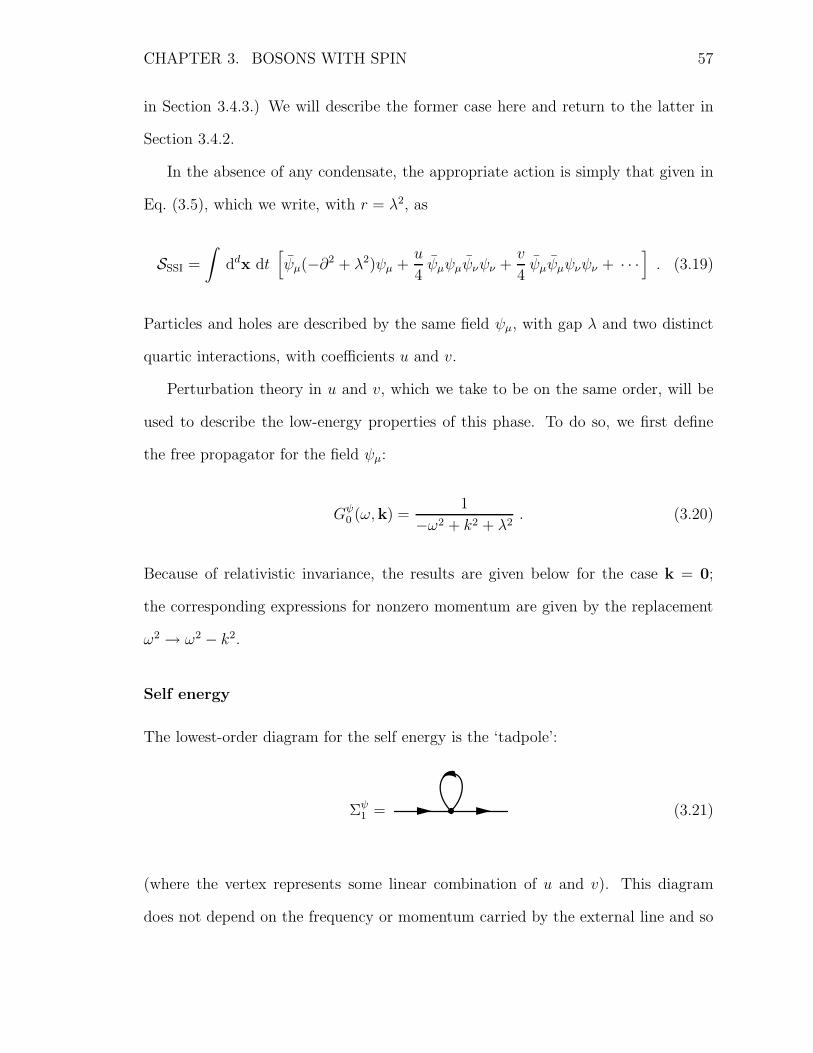
CHAPTER 3. BOSONS WITH SPIN 57
in Section 3.4.3.) We will describe the former case here and return to the latter in
Section 3.4.2.
In the absence of any condensate, the appropriate action is simply that given in
Eq. (3.5), which we write, with r = #2, as
SSSI =
!ddx dt
-&µ((22 + #2)&µ +
u
4&µ&µ&)&) +
v
4&µ&µ&)&) + · · ·
.. (3.19)
Particles and holes are described by the same field &µ, with gap # and two distinct
quartic interactions, with coe#cients u and v.
Perturbation theory in u and v, which we take to be on the same order, will be
used to describe the low-energy properties of this phase. To do so, we first define
the free propagator for the field &µ:
G"0 (%,k) =
1
(%2 + k2 + #2. (3.20)
Because of relativistic invariance, the results are given below for the case k = 0;
the corresponding expressions for nonzero momentum are given by the replacement
%2 " %2 ( k2.
Self energy
The lowest-order diagram for the self energy is the ‘tadpole’:
&"1 = (3.21)
(where the vertex represents some linear combination of u and v). This diagram
does not depend on the frequency or momentum carried by the external line and so

CHAPTER 3. BOSONS WITH SPIN 58
simply contributes a constant that renormalizes the gap #.
The lowest-order diagram that depends on the external momentum is
&"2 = . (3.22)
The physical interpretation of this diagram is as the decay of a particle, given suf-
ficient energy, into a hole (described by the top line, with reversed propagation
direction) and two particles. It is therefore clear that this diagram will make no
contribution to the decay rate for a particle unless its energy exceeds 3#.
This interpretation is clarified by using the spectral representation; the ‘spectral
weight’ is given by
$"(%) = 2 lim$(0+
Im G"(% + i)) , (3.23)
where G" is the full propagator. This can be calculated numerically, and is shown in
Fig. 3.2.4 There is a delta-function peak at % = # (a small width has been manually
added to make it visible on the plot), and a three-body continuum, resulting from
&"2 , appears at % = 3#.
3.4.2 SSI near SSC
As the spin-dependent interaction increases and the SSC phase is approached, a
bound state composed of a singlet pair of bosons becomes energetically favorable.
At the transition to SSC, the singlet pairs condense into a superfluid with no spin
4We note here a subtlety regarding this plot and those in the remainder of Section 3.4. Thefull series of diagrams, including those shown in Eq. (3.21) and Eq. (3.22), cause a renormalizationof the gap % (and hence movement of the features in &") away from its bare value, ie, the valueappearing explicitly in the action. In this plot (and the ones that follow), % should be interpretedas meaning the renormalized value, rather than the bare value, and it is for this reason that thepeak appears precisely at ' = %.

CHAPTER 3. BOSONS WITH SPIN 59
Frequency %/#
Spec
tral
wei
ght$"
76543210
Figure 3.2: The spectral weight $" in SSI, calculated up to second order in thecouplings u and v. The delta-function peak at % = # (which has artificially beengiven a small but nonzero width) describes the stable particle excitation of the field&µ. For % > 3#, there is continuum of three-particle excitations.
ordering.
To describe the approach to this transition, we start with the action SSSI and
introduce the field " ) &µ&µ, by a Hubbard-Stratonovich decoupling of the quartic
interaction v. The field " describes the singlet pairs and will condense across the
transition. It is described by the action
S! =
!ddx dt
(|2"|2 + r!|"|2 +
u!4|"|4 + · · ·
). (3.24)
The full action has the form
S %SSI = S" + S! +
g"2
!ddx dt
/"&µ&µ + "&µ&µ
0. (3.25)
(The introduction of the field " renormalizes the coupling constants within S". Here
and throughout, we will simplify the notation by retaining the same symbols for these

CHAPTER 3. BOSONS WITH SPIN 60
renormalized quantities.)
Self energy
The diagrams shown in Section 3.4.1, coming from S", will still contribute to the
self energy near to SSC. As seen above, however, these diagrams are important only
for % > 3#, whereas new diagrams coming from coupling to the pair field " will
contribute at lower frequencies.
Using a dashed line for the propagator of the " field, the first such diagram is
&"1 = , (3.26)
in which a particle decays into a hole plus a pair. The vertices correspond to factors
of g". The threshold for this process is clearly # + #!, where # is the gap to the
particle and hole excitation as before, and #! =3
r! is the gap to the pair excitation.
This excitation therefore becomes important at low energies when #! < 2#, which
is simply the condition that a bound state exists below the two-particle continuum.
The diagram can be evaluated to give
&"1 =
g2"
8-%log
#+ #! + %
#+ #! ( %, (3.27)
and the corresponding spectral weight is shown in Fig. 3.3. A continuum of excita-
tions appears for % > #+#!, as expected. As the transition to SSC is approached, #!
becomes smaller and the edge of the continuum approaches the peak at % = #. The
perturbation expansion used here breaks down as #! " 0 and a more sophisticated
RG calculation, described in Section 3.5.1, is required.

CHAPTER 3. BOSONS WITH SPIN 61
#!/# = 0.15#!/# = 0.10#!/# = 0.05
Frequency %/#
Spec
tral
wei
ght$"
1.51.41.31.21.110.9
Figure 3.3: The spectral weight $" in SSI near the transition to SSC, calculated upto order g2
", plotted for three di!erent values of #!, the gap to pair excitations. Thecoupling strength is g" = 0.1. The peak at % = # (which is present for all values of#! and has artificially been given a small but nonzero width) describes the stableparticle and hole excitation of the field &µ. For % > # + #!, there is continuum ofexcitations, corresponding physically to the conversion of a particle to a pair plus ahole.

CHAPTER 3. BOSONS WITH SPIN 62
3.4.3 Spin-singlet condensate
In the SSC phase, singlet pairs of bosons form a condensate, giving a superfluid with
no spin ordering. The perturbation expansion used in Section 3.4.2 is not applicable
here, and we must instead expand about the new ground state, with a condensed
" field. (A similar approach can be used to describe the condensed phase of the
spinless Bose gas [86].)
We first write " in terms of amplitude and phase as
" = "0ei+! , (3.28)
where "0 and (% are both real. For simplicity, we treat the amplitude of the " field as
a constant, ignoring the gapped amplitude modes. (This is appropriate su#ciently
far from the transition to SSI, where the gap is large.) With this parameterization,
S!, given by Eq. (3.24), can be rewritten as the action of a free, gapless field:
S! =
!ddx dt
1
2(2()2 , (3.29)
with the definition ( =3
2"0(%. Physically, ( is interpreted as the Goldstone mode
corresponding to the broken phase symmetry in SSC.
In dealing with &µ, it is convenient to take out a factor of the condensate phase
by writing &µ = 'µei+!/2. Then, since the condensate has broken phase-rotation
invariance, we rewrite the field 'µ in terms of real and imaginary parts,
'µ =132('R
µ + i'Iµ) . (3.30)

CHAPTER 3. BOSONS WITH SPIN 63
In terms of the new fields (, 'Rµ and 'I
µ, the action becomes5
SSSC =
!ddx dt
C1
2(2()2 +
1
2'R
µ ((22 + r + g""0/2)'Rµ
+1
2'I
µ((22 + r ( g""0/2)'Iµ +
u
16('R
µ'Rµ + 'I
µ'Iµ)('R
) 'R) + 'I
)'I))
+v
16
2('R
µ'Rµ ( 'I
µ'Iµ)('
R) '
R) ( 'I
)'I)) + 4'R
µ'Iµ'
R) '
I)
3
+i38"0
('Iµ2'
Rµ ( 'R
µ2'Iµ) · 2( +
1
16"20
('Rµ'
Rµ + 'I
µ'Iµ)(2()2
D. (3.31)
Note that the two fields 'Rµ and 'I
µ remain gapped, but that their gaps are no longer
the same. The lowest-energy ‘charged’ mode is 'Iµ, with gap #I =
4r ( g""0/2.
Self energy
As an example, we consider the lowest-order diagram that contributes to the self
energy for 'Iµ, at energies well below that required to produce an excitation of the
field 'Rµ . This is given by
&# = , (3.32)
where the solid lines represent 'Iµ and the dashed lines (. Each vertex represents a
factor ) (p1 · p2)"!20 , where p1 and p2 are the momenta of the two ( propagators,
coming from the final term in SSSC. (All the other interaction terms involve 'Rµ and
contribute to the decay rate only at higher energies. As in Section 3.4.1, there is also
a lower-order tadpole diagram that does not contribute to the decay rate.)
The diagram can be calculated numerically and the corresponding spectral weight
5It is straightforward to show that the Jacobian associated with the change of variables is equalto a constant.

CHAPTER 3. BOSONS WITH SPIN 64
Frequency (% ( #I)/#I
Spec
tral
wei
ght$#
0.30.250.20.150.10.050(0.05(0.1
Figure 3.4: The spectral weight $# for the field 'Iµ in SSC, near the gap #I , calcu-
lated numerically using the diagram in Eq. (3.32). As in Figs. 3.2 and 3.3, there isa delta-function peak at % = #I (which has artificially been given a nonzero width),corresponding to the stable particle excitation. In this case, unlike in SSI, the con-tinuum in the spectral weight occurs immediately above the peak. This is due tothe (gapless) Goldstone mode ( resulting from the broken phase symmetry in SSC.The derivatives in the coupling between the Goldstone mode and the 'I
µ field in SSSC
strongly suppress the spectral weight as % " #I from above; in fact, $# ) (%( #I)3.
is shown in Fig. 3.4. As in SSI, there is a sharp peak (at % = #I) corresponding
to the stable gapped ‘charged’ mode, followed at higher energy by a continuum of
excitations. In this case, however, the Goldstone mode ( causes the continuum to
begin precisely at % = #I , albeit suppressed by a factor of (% ( #I)3.
This should be contrasted with the transition between SSI and SSC, described
below in Section 3.5.1. At the transition, the gapless modes are critical, rather than
Goldstone modes, and their coupling is not suppressed by powers of the momentum.
As a result, the spectral weight, calculated perturbatively, does not tend to zero as
% " # (see Section 3.5.2) and a RG analysis shows that the sharp peak at % = # is
in fact replaced by a weaker singularity.

CHAPTER 3. BOSONS WITH SPIN 65
3.5 Critical properties
The critical field at the transition to SSC is the singlet pair ", introduced in Sec-
tion 3.4.2. Once " has been isolated, &µ, which has no gapless excitations, can be
safely integrated out. This leaves the field theory of a single complex scalar, with
the same form6 as the action S! given in Eq. (3.24):
S! =
!ddx dt
(|2"|2 + r!|"|2 +
u!4|"|4 + · · ·
). (3.33)
This transition is therefore of the XY universality class, with upper critical dimension
D = d + 1 = 4. (The field " has engineering dimension ["] = (d ( 1)/2, so the
coupling u! has dimension [u!] = 3 ( d.)
While the action S! is su#cient to describe the critical properties of the ground
state across the transition, we are also interested in the behavior single-particle
excitations, and other excitations that carry spin. Since " is spinless, the critical
theory given by S! does not describe these. Instead, we must keep the singly-charged
excitations given by &µ, and use the full action S %SSI, in Eq. (3.25).
Since &µ has only gapped excitations, while the field " is now gapless, this can
be simplified somewhat. The important excitations are those just above the gap
# =3
r, for which the dispersion can be replaced by a nonrelativistic form. We
define particle and hole operators so that &µ ) pµ + hµ, giving an action S! + S %!,",
6Integrating out the field "µ renormalizes the constants in S!. We will retain the same symbolsfor the renormalized quantities, because we are interested in the critical behavior, which is describedby a fixed point of the action and is not dependent on the precise values of the parameters.
CHAPTER 3. BOSONS WITH SPIN 66
where
S %!," =
!ddx dt
&pµ
$i2t (
*2
2m"+ #
%pµ + hµ
$i2t (
*2
2m"+ #
%hµ
+ g"/"pµhµ + "pµhµ
0 '. (3.34)
Using power counting (and taking [t] = [x] = (1, since the critical theory S! is
relativistic), the engineering dimension of the kinetic-energy term is [1/m"] = (1.
The dispersion is therefore irrelevant and the particles and holes can be treated as
static impurities. This gives, finally,
S!," =
!ddx dt
2pµ (i2t + #) pµ + hµ (i2t + #)hµ + g"
/"pµhµ + "pµhµ
03. (3.35)
The scaling dimension of the coupling g" is [g"] = (3(d)/2, so that it is relevant
for d < 3. It is therefore relevant in two (spatial) dimensions and marginal in three,
and we will consider both of these cases below. Any other interactions, including
terms quartic in pµ and hµ, are irrelevant.
In Section 3.5.1, we will treat the case d = 2 using a renormalization-group (RG)
analysis, and then, in Section 3.5.2, return to the case d = 3, where straightforward
perturbation theory is su#cient.
3.5.1 Renormalization group
For d < 3, the correlation functions of the particle and hole excitations can be found
using a RG calculation. Since the present approach is slightly di!erent from the
standard RG, we perform the calculation using a cuto! in momentum space, which
makes the logic involved more transparent, in Section A.3 of the appendix. Here we
use dimensional regularization, which is the simplest approach from a calculational
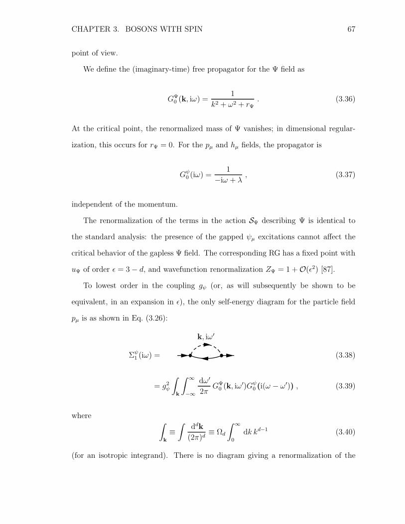
CHAPTER 3. BOSONS WITH SPIN 67
point of view.
We define the (imaginary-time) free propagator for the " field as
G!0 (k, i%) =
1
k2 + %2 + r!. (3.36)
At the critical point, the renormalized mass of " vanishes; in dimensional regular-
ization, this occurs for r! = 0. For the pµ and hµ fields, the propagator is
G"0 (i%) =
1
(i% + #, (3.37)
independent of the momentum.
The renormalization of the terms in the action S! describing " is identical to
the standard analysis: the presence of the gapped &µ excitations cannot a!ect the
critical behavior of the gapless " field. The corresponding RG has a fixed point with
u! of order * = 3 ( d, and wavefunction renormalization Z! = 1 + O(*2) [87].
To lowest order in the coupling g" (or, as will subsequently be shown to be
equivalent, in an expansion in *), the only self-energy diagram for the particle field
pµ is as shown in Eq. (3.26):
&"1 (i%) =
k, i%%
(3.38)
= g2"
!
k
! &
!&
d%%
2-G!
0 (k, i%%)G"0 (i(% ( %%)) , (3.39)
where!
k
0!
ddk
(2-)d0 *d
! &
0
dk kd!1 (3.40)
(for an isotropic integrand). There is no diagram giving a renormalization of the

CHAPTER 3. BOSONS WITH SPIN 68
coupling g" at this order, so this is the only diagram that must be evaluated.
Performing the integral over %% using contour integration gives
&"1 (i%) = g2
"
!
k
1
2k·
1
(i% + #+ k, (3.41)
which leads to, defining z = (i% + #,
&"1 (i%) = (
g2"z1!,
4-2*, (3.42)
plus terms that are finite as *" 0.
To this order, the full propagator of the particle is then given by
(G")!1 = z ( &"1 (3.43)
= z
$1 +
g2"z!,
4-2*
%, (3.44)
so that renormalizing the propagator (using minimal subtraction) at real frequency
z = µ gives for the wavefunction renormalization
Z" = 1 (g2"µ!,
4-2*. (3.45)
Since there are no diagrams corresponding to renormalization of the coupling, we
have Zg = 1, to this order.
We now define the (dimensionless) renormalized coupling g", given by
g" = 2-g"µ,/2Zg
Z"
3Z!
. (3.46)
In terms of this, we have Z" = 1 ( g2"/*, and the beta function for the coupling is

CHAPTER 3. BOSONS WITH SPIN 69
given by
.(g") 0 µ
$2g"2µ
%
g!
= g"((*
2+ g2
"
), (3.47)
so that the fixed point is at
g!" =
,*
2. (3.48)
Since the fixed point has g!" ) *1/2, a perturbative expansion at this point is indeed
equivalent to an expansion in *.
The anomalous dimension of the particle (and hole) propagator is then given by
)" = .d
dg"log Z" , (3.49)
so that )" = */2 at the fixed point.
We have also obtained results for the next order in this expansion [70], which also
involves diagrams renormalizing the coupling g". The fixed point then occurs at
(g!")2 =1
2*(
$-2
15(
49
100
%*2 + O(*3) , (3.50)
and the anomalous dimension is
)" =1
2*+
$-2
15(
6
25
%*2 + O(*3) . (3.51)
The Green function behaves, for % > #, as
G"(%) ) (#( %)!1+$! , (3.52)

CHAPTER 3. BOSONS WITH SPIN 70
Frequency %/#
Spec
tral
wei
ght$"
32.521.510.50
Figure 3.5: The spectral weight $" at the SSI–SSC transition in d = 2 spatialdimensions. The delta-function peak at % = # has been replaced by a continuumof excitations, with $" ) (% ( #)!1+$! . The numerical value )" = 0.91797 used inthe plot results from a dimensional expansion in * = 3 ( d, carried out to order *2,Eq. (3.51), and evaluated at * = 1.
so that the corresponding spectral weight is given by
$"(%) ) (% ( #)!1+$! . (3.53)
The relativistic invariance of the original theory allows these results to be extended
to finite external momentum by the usual replacement % "3%2 ( k2.
Figure 3.5 shows the spectral weight $" for d = 2 (* = 1), using the numeri-
cal value from Eq. (3.51). The quasiparticle peak appearing on both sides of the
critical point (see Figs. 3.2, 3.3 and 3.4) is replaced by an incoherent continuum of
excitations.

CHAPTER 3. BOSONS WITH SPIN 71
Higher-order response functions
A similar calculation applies to the response functions corresponding to composite
operators, such as those of the form Tµ)pµh) . These operators, where Tµ) is an
arbitrary matrix, correspond to excitations that are chargeless, but (assuming Tµ) &=
0µ)) carry net spin. Such composite operators will be represented by the following
‘insertion’:&)
&µ
(3.54)
To find the critical exponent for these compound operators, we must consider
renormalization of the corresponding insertion, given (at one-loop order) by the di-
agram
H1(2i%) = k, i%% (3.55)
= g2"
!
k
! &
!&
d%%
2-G!
0 (k, i%%)G"0 (i(% ( %%))G"
0 (i(% + %%)) , (3.56)
where all spin indices have been omitted. The integral can be performed to give
H1(2i%) = (g2"z!,
4-2*. (3.57)
In accounting for the spin indices, it is important to note that the exchange of
the pair interchanges the particle and hole lines and hence the indices µ and !. This
causes the results to be dependent on the symmetry of the matrix Tµ) , leading to
di!erent exponents y2± for excitations of even (Tµ) symmetric) and odd spin (Tµ)

CHAPTER 3. BOSONS WITH SPIN 72
antisymmetric). Including the two-loop results, we have, for the former,
y2+ = 1 ( *+
$2-2
15(
49
50
%*2 + O(*3) , (3.58)
while y2! = 1 exactly for the latter [70].
In terms of this exponent, the correlation function behaves like
+µ),*%(2%) ) (#( %)!y2 . (3.59)
Of particular importance is the spectral density
Aµ),*%(2%) = lim$(0+
Im+µ),*%(2% + i)) , (3.60)
which is a delta-function at % = # for y2 = 1, and otherwise behaves like
Aµ),*%(2%) ) (% ( #)!y2 , (3.61)
for % just above the gap #.
3.5.2 Perturbation theory
For d = 3, the fixed point of the RG equations occurs for g!" = 0, so perturbation
theory in the coupling can be used to determine the structure of the Green function.
Using the fully relativistic form of the action to calculate the lowest-order self-energy
diagram gives, for %2 > #2 + k2,
Im&"d=3 =
g2"
8-·%2 ( k2 ( #2
%2 ( k2. (3.62)

CHAPTER 3. BOSONS WITH SPIN 73
Frequency %/#
Spec
tral
wei
ght$"
32.521.510.50
Figure 3.6: The spectral weight $" at the SSI–SSC transition in d = 3 spatialdimensions. The delta-function peak at % = # has been replaced by a continuum ofexcitations, with the mean-field exponent $" ) (% ( #)!1.
For comparison, the same calculation in two dimensions gives
Im&"d=2 =
g2"
8·
13%2 ( k2
. (3.63)
(Im&" = 0 for %2 < #2 +k2 in both cases.) Note that Im&"d=2 tends to a constant as
% "3#2 + k2 from above, in contrast to the cases considered in Section 3.4 above.
The same is not true in three dimensions, and we have
Im&"d=3 ) % (
3#2 + k2 . (3.64)
The corresponding spectral weight for the particle and hole excitations is shown
in Fig. 3.6. As in Fig. 3.5, the coherent quasiparticle peak is replaced by a continuum
of excitations, but the exponent is given by its mean-field value: $" ) (% ( #)!1.
CHAPTER 3. BOSONS WITH SPIN 74
3.6 Conclusions
In this chapter, we have considered a system of bosons with spin in a lattice potential,
which can be experimentally realized using atoms trapped in an optical lattice. Using
the Bose-Hubbard model, extended to the case with spin, it was argued that the
system allows for both spin and phase ordering. In order to have superfluidity (phase
ordering) without breaking spin-rotation symmetry, it is necessary to condense singlet
pairs of bosons. Such a condensed state, referred to as the spin-singlet condensate
(SSC), and, in particular, the transition to this state from the featureless spin-singlet
insulator (SSI), was the main focus of the chapter.
A simple mean-field theory was constructed containing the physics of these pha-
ses, by allowing explicitly for the possibility of a condensate of singlet pairs. The
phase diagram (Fig. 3.1) found by this method illustrates, as expected, that the SSC
is favored for su#ciently strong spin-dependent interactions.
We then turned to the description of the SSI and SSC phases in terms of their
low-energy excitations. Within the insulating phase, all excitations are gapped (ie,
occur at finite energy above the ground state), whereas in the condensate a gapless
Goldstone mode appears, corresponding to the broken gauge symmetry. In both
phases, there is a singly-charged, spin-carrying excitation corresponding to a single
particle or hole, giving an infinitely sharp peak in the spectral weight. This excitation
remains gapped in the SSC, where singlet pairs of particles, rather than the individual
bosons, condense.
At the transition, a calculation using the renormalization group (RG) was used to
show that this sharp peak is replaced by an incoherent continuum of excitations. This
results from the strong coupling to the gapless critical modes at the transition. Using
scaling arguments, it was shown the dispersion of the gapped particle excitation is

CHAPTER 3. BOSONS WITH SPIN 75
irrelevant (in the RG sense) and that the corresponding response function can be
found by treating it as a static impurity. The anomalous exponents were then found
using a dimensional expansion.
While the analysis here has addressed the specific case of bosons with spin, it
should be noted that the results regarding the critical properties can be applied
directly to other paired condensates. The results rely on the existence of a gap to
single-particle excitations and on particle–hole symmetry near the transition, but are
otherwise quite general. In Section 4.5, we describe other examples where similar
results are expected.

Chapter 4
Summary and outlook
This thesis has presented theoretical analyses of two systems that might previously
have been considered purely hypothetical models, but can now potentially be realized
using techniques for manipulating ultracold atoms.
In the first system, a Bose-Fermi mixture with a Feshbach resonance, a phase
diagram was constructed using mean-field theory, showing how simple energetic con-
siderations and quantum-mechanical e!ects allow for a variety of phases. We then
demonstrated that these phases could be distinguished by their di!erent Luttinger
constraints. Techniques from quantum field theory were used to describe the transi-
tions between the phases and to investigate the validity of the mean-field theory.
For the second system, a collection of bosons with spin confined within an optical
lattice, considerations of symmetry were used to classify the various possible phases
and a simple mean-field theory was constructed to serve as a guide to the phase
structure in the regime of interest. We then addressed the behavior of excitations
carrying spin at the appearance of a spin-singlet condensate. Considerations based
on the renormalization group, and a calculation using an expansion in the spatial
dimensionality, allowed the critical behavior of such excitations to be determined.
76

CHAPTER 4. SUMMARY AND OUTLOOK 77
I now describe some recent related experimental results, limitations of the analysis
presented above, and potential future directions for related research.
4.1 Bose-Fermi mixtures: recent experiments
In recent experiments [41], the possibility of tuning a Feshbach resonance between
fermionic and bosonic atoms has been demonstrated using a mixture of potassium-40
(fermion) and rubidium-87 (boson). These experiments also provide good evidence
for the formation of bound molecular states as the detuning is slowly reduced from
large positive values.
Unfortunately, it appears that the scattering rate between the fermionic molecules
and the residual bosonic atoms is su#ciently high that the lifetime of the molecules
within the trap is extremely short. This scattering has been omitted from the analysis
in Chapter 2.
It is nonetheless interesting to consider the appearance of these molecules, which
occurs at the line separating ‘1 FS + BEC’ and ‘2 FS + BEC’ on the right-hand side
of Fig. 2.3 (on p. 24). To the right of this line, molecules are absent and the loss rate
of atoms is low; crossing the line causes the formation of molecules and a significant
loss of atoms from the trap.
Further experiments are planned [88] to map out the boundary as a function
of detuning, temperature and the relative atomic numbers. A theoretical analysis
beyond mean-field and incorporating the di!erent spatial-density profiles of the two
atomic species might be necessary for closer agreement with these experiments.

CHAPTER 4. SUMMARY AND OUTLOOK 78
4.2 Universality in quantum liquids
Recent work [25] has shown that certain properties of quantum liquids at large scat-
tering lengths, where their behavior displays universality, can be understood in terms
of renormalization group (RG) flows. An expansion in the spatial dimensionality [89],
similar to that described in Section 3.5.1, can be used to give explicit expressions for
the universal functions.
An analysis of the case of pairing between fermions has been carried out [25] using
this dimensional expansion and another technique useful for strongly interacting
systems, the ‘1/N expansion’. It would be interesting to apply these techniques to
access the universal phase diagram for Bose-Fermi mixtures.
4.3 Extensions of Luttinger’s theorem in related
systems
A feature of particular novelty in the Bose-Fermi mixture is the appearance of dif-
ferent forms of Luttinger’s theorem within the di!erent phases. As described in
Chapter 2, this comes about because of the separate conservation laws governing the
two species of atoms. In the absence of a BEC, all of the atoms are contained within
Fermi surfaces, resulting in two separate Luttinger constraints, while the presence of
a condensate eliminates one of the two.
These results can in fact be extended to other systems involving multiple species
of fermions, and an example is provided by fermion pairing [90] (see also Section 1.1).
In the case when the densities of the two fermion species (for example, two spin states)
are unequal, a paired condensate can coexist with one or more Fermi surfaces. This
case is analogous to the phases ‘1 FS + BEC’ and ‘2 FS + BEC’ of Chapter 2, and

CHAPTER 4. SUMMARY AND OUTLOOK 79
a single Luttinger constraint again applies, in this case to the di!erence of the Fermi
surface volumes. In the absence of condensate, the two Fermi surfaces’ volumes are
separately constrained, as in the phase ‘2 FS, no BEC’.
Another, seemingly unrelated, system to which similar considerations apply is
the Kondo lattice model of the heavy-fermion compounds [91–93]. In this model,
electrons in localized f orbitals interact with those of the conduction band, and
two number constraints can again be formulated. The connection can be made
more explicit by introducing a boson to represent hybridization between the orbitals;
condensation of this boson corresponds to the standard heavy Fermi liquid with a
single Luttinger constraint.
4.4 Assumption of spatial uniformity
An important simplification that we have made throughout our analysis of both
models is to assume spatial uniformity, while in actual experiments, it is necessary
to confine the atoms using an external trapping potential. In the case of an optical
lattice, this trap is superimposed upon the lattice potential and can have significant
e!ects, which have been studied using numerical approaches [94,95]. The main e!ect
is to replace the uniform insulator state by a shell structure, where regions closer to
the center of the potential have higher occupation numbers than those further out.
Adding a trapping potential [31] to models formulated in the continuum (such
as the Bose-Fermi mixture of Chapter 2) causes the single-particle states to cease to
be pure momentum states, with relatively minor quantitative e!ects on the phase
structure. Luttinger’s theorem, however, now applies in the new single-particle basis,
and the momentum-space distribution has no discontinuity. It may, however, be
possible to modify the trapping potential to produce one that approximates a square

CHAPTER 4. SUMMARY AND OUTLOOK 80
well [90], for which the single-particle states again have well-defined momentum. This
would allow the Fermi surface to be seen directly in the time-of-flight measurements
described in Chapter 1.
4.5 Excited-state spectra at other pairing transi-
tions
The results found in Chapter 3 for pairing transitions of bosons with spin can also be
applied, with minor modifications, to the case of fermions. It was assumed through-
out, however, that single-particle excitations were gapped on both sides of the pairing
transition, and so the results are not applicable to the standard BCS transition from
a gapless Fermi liquid.
Instead, consider a band insulator, with an integer number of fermions per spin
state, per site of the lattice. At su#ciently strong attractive interactions between the
fermions, this state undergoes a transition into a paired condensate, which is directly
analogous to the SSC of Chapter 3. In both states, the single-particle excitations
remain gapped as in the bosonic case.
As can be seen in Section 3.5.1, the critical properties of the gapped excitations
are determined by diagrams with only one single-particle line. The bosonic nature
of that particle is therefore unimportant and the results for the Green function G"
can be applied without modification to fermions. In the case of the two-particle
response functions, the same results again apply, but with the roles of symmetric
and antisymmetric matrices Tµ) reversed.
Besides atoms in optical lattices, our results also apply to superfluid-insulator
transition in electronic systems, provided that there is an even number of electrons
per unit cell. Such a situation can arise in the cuprate compounds, with a periodic

CHAPTER 4. SUMMARY AND OUTLOOK 81
potential generated spontaneously by charge-density-wave order. For example, recent
experiments in spin ladder compounds [96] have shown that each unit cell of the
‘stripe’ ordering pattern contains a pair of holes. The results of Chapter 3 then
predict the frequency dependence of the electron photoemission spectrum across a
superfluid-insulator transition in which the charge-density wave is present on both
sides of the transition [70].
4.6 Other transitions of spinful bosons in optical
lattices
In Chapter 3, the phase diagram of bosons with spin in optical lattices has been
investigated and shown to contain a number of phases. The transition from an
insulating state to a paired superfluid was the subject of our focus, because the
presence of (unbroken) spin-rotation symmetry on both sides of the transition leads
to interesting response functions for operators that carry spin.
More generally, the behavior of such response functions across the transitions
shown in Fig. 3.1 will depend on the order parameter governing each transition.
For example, the transition between the phases SSI and PC has an order parameter
carrying nonzero spin. The spin-excitation spectrum is then gapless at the critical
point and the standard methods of quantum critical phenomena can be used to
determine the scaling dimensions. We intend to investigate this and other cases in
more detail in future work.

Appendix
A.1 Dressed molecular propagator
In Chapter 2, we have considered the many-body physics of the model defined in
Section 2.2. In this section, we will consider an isolated molecule, and find an
expression for the renormalized (‘dressed’) molecular propagator [24, 75], involving
all orders in the coupling g.
A.1.1 Diagrammatic description
An isolated bosonic or fermionic atom in the vacuum is an exact eigenstate of
the Hamiltonian, Eq. (2.4), since the interaction terms in Hint annihilate such a
state. The same is not, however, true of a molecule, for which the process shown in
Eq. (2.64), which can take place in the vacuum, produces a correction to the prop-
agator. The dressed molecular propagator can be found using the Dyson equation,
which can be written diagrammatically for this case as
&=
&+
&
b
f&
(A.1)
82
APPENDIX 83
where only the term in the bubble diagram Eq. (2.64) of order zero in density is to
be included.
A.1.2 Calculations
The Dyson equation Eq. (A.1) gives the relation between the reciprocals of the bare
and full Green functions
9("q = ("
q (g2
.
#
p
Gfq!pG
bp ; (A.2)
compare Eq. (2.53).1
In the vacuum, both the Bose-Einstein and Fermi-Dirac factors give zero, leaving
9("q = ("
q ( g2
!d3k
(2-)3
51
,bk
+ ,fk!!k
( i%(
2mfmb
m"k2
6
, (A.3)
where q stands for k% and %, the (imaginary-time) frequency. (The second term in
the parentheses comes from renormalizing the detuning !, as in Section 2.7.1.) The
integral can be performed analytically, to give
9("q = ("
q + 2"E,"k! ( ! ( i% , (A.4)
where ", defined in Eq. (2.7), has been used.
This function can be continued to one that is analytic everywhere except along
the real axis, by replacing i% by z. In terms of z, the full Green function is
9G"k!(z) =
1
(z + ,"k! + 2"
E,"k! ( ! ( z
. (A.5)
1The sign di#erence results from the fermion loop in Eq. (2.51).

APPENDIX 84
Along the real axis, the square root has a branch cut for z > ,"k!(! which corresponds
to the continuum of free-atom excitations. For ! < 0, 9G" has a single pole at the
real value
z0 = ,"k! ( 2"
(" (
4"2 ( !
), (A.6)
corresponding to the renormalized molecule. For ! > 0, there are no poles, since the
molecule has a finite lifetime, decaying into two atoms.
A.1.3 Spectral representation
These analytical properties are best summarized using the spectral representation
for 9G",
9G"k!(z) =
! &
!&
dx
2-
$"k!(x)
x ( z. (A.7)
The spectral weight, defined in Eq. (3.23), is in this case given by
$"k!(x) = '(x ( ,"
k! + !)4"E
x ( ,"k! + !
/x ( ,"
k!
02+ 4"2
/x ( ,"
k! + !0
+ '((!)4"2 ( ! ( "4"2 ( !
2-0(((x ( ,"
k! ( 2"/4
"2 ( ! ( "0)))
, (A.8)
where ' is the unit step function and 0 is the Dirac delta function. A plot of $"0 (x)
is shown for "2/T0 = 2.5 # 10!4 in Fig. A.1 and for "2/T0 = 0.1 in Fig. A.2. In
both cases, there is a delta-function peak at some x < 0 only for negative !, and a
continuum of excitations for x > 0 for all ! (although this is too small to be visible
in Fig. A.1 for !/T0 = (1). In the case where "2/T0 = 2.5# 10!4, there is a narrow
well-defined peak in the spectral weight for ! > 0, corresponding to a long-lived
molecular state; it is for this reason that we refer to this case as a ‘narrow’ Feshbach
resonance. For "2/T0 = 0.1, the same peak is much broader, corresponding to a

APPENDIX 85
!/T0 = 1!/T0 = 0!/T0 = (1
Energy x/T0
Spec
tral
wei
ght$" 0
(x)
2.521.510.50(0.5(1(1.5
Figure A.1: The spectral weight $"0 of the molecule in vacuum for a narrow Feshbachresonance, with "2/T0 = 2.5 # 10!4, for three di!erent detunings. (The density iszero in this plot, so T0 is an arbitrarily chosen unit of energy.) The curves have allbeen evaluated at zero momentum; a nonzero momentum k would simply shift thecurves to the right by an amount k2/(2m"). For ! < 0, there is a delta-functionpeak for negative x, which has artificially been given a finite width. For all !, thereis a continuum for x > 0, but this is too small to be visible for !/T0 = (1.
shorter lifetime for decay into a pair of atoms.
Note that, while the expression for $"k! depends on the momentum k%, the latter
appears only in the combination x(,"k! and we have therefore kept k% = 0 for clarity.
(We have similarly set µ" = 0, which in the present case simply corresponds to a
choice of the zero of energy.)
Weak-coupling limit
As the coupling strength is reduced, the peak shown in Fig. A.1 for x > 0 and ! > 0
becomes progressively narrower. In the limit " " 0, the first term of Eq. (A.8)
involves the Lorentzian representation of the Dirac delta function,
lim-(0
4
t2 + 42= -0(t) . (A.9)

APPENDIX 86
!/T0 = 1!/T0 = 0!/T0 = (1
Energy x/T0
Spec
tral
wei
ght$" 0
(x)
43.532.521.510.50(0.5(1
Figure A.2: As Fig. A.1, but for a broader resonance, "2/T0 = 0.1.
For " small enough, the first term of Eq. (A.8) thus has weight only near x = ,"k!,
where x ( ,"k! + ! can be replaced by !. The limit of vanishing " is therefore given
by
lim.(0
2"E
x ( ,"k! + !
(x ( ,"
k!
)2+ 4"2
(x ( ,"
k! + !) = -0(x ( ,"
k!) , (A.10)
so that the spectral weight becomes, in this limit,
$"k!(x) " '(x ( ,"
k! + !)0(x ( ,"k!) + 2-'((!)0(x ( ,"
k!)
= 2-0(x ( ,"k!) ,
(A.11)
which, with Eq. (A.7), gives the free propagator for the bare molecule, as used in
Section 2.6.

APPENDIX 87
A.2 Stability against phase separation
The results of Chapter 2 rely on the assumption that the ground state is always a
homogeneous mixture of bosons, fermions and molecules. In this section, we address
the question of whether the Bose-Fermi mixture is stable to separation into multiple
regions with di!erent densities. We use the mean-field results of Section 2.4. and,
for simplicity, the temperature will be taken as zero throughout.
Note that we are only allowing for instabilities allowed by the explicit model H,
given in Eq. (2.4). Other interaction terms that we have omitted may also lead to
instabilities; see Section 4.1.
A.2.1 The compressibility matrix
To establish the stability of the system against separation into two coexisting fluids,
we evaluate the compressibility matrix [97], defined by
K %/& = (
22%
2µ/2µ&, (A.12)
for 1, . 1 {f, b}.
We now define the (canonical) free energy F (Nf , Nb) by a Legendre transforma-
tion,
F (Nf , Nb) = %(µf , µ") + µfNf + µbNb , (A.13)
where Nf and Nb are the total number of Fermi and Bose atoms, respectively. (Note
that the full fermion and boson numbers, which are conserved by the Hamiltonian, are
used.) The compressibility matrix K % is then the inverse of the Hessian of F , so that
complete stability against phase separation requires that K % be positive semidefinite.
It is in fact easier to work with the matrix K/&, given by the same expression,

APPENDIX 88
Eq. (A.12), but with 1, . 1 {f,&}. This amounts to a simple (but not orthogonal)
change of basis; it is su#cient (and necessary) for K % to be positive semidefinite that
K be the same.
We begin with Eqs. (2.19) and (2.20), and use Eq. (2.26) to determine the implicit
dependence of ' on the chemical potentials. We must then take second derivatives
with respect to the two chemical potentials to find the compressibility matrix. In
the presence of a condensate, this leads to an expression
K/& = K(0)/& +
r/r&
#, (A.14)
where K(0)/& is the matrix of second derivatives, evaluated at fixed ' and r/ is a
function whose form will not concern us here.
The denominator of the second term is
# = #+ g4
! k!0
kF0
dn(k)
W 3k
(1
2g4/zF + z!
0, (A.15)
where
zx =m"mf dn/ dk
k(,fk + ,"k
)(mf,f
k + m","k
)
111111k=kx
0
(A.16)
and
Wk =
,(,fk ( ,"k
)2+ 4g2'2 . (A.17)
When # goes through zero, the determinant of K diverges, so that the Hessian of
F becomes singular, signifying that one of its eigenvalues vanishes. This marks the
onset of instability; we conclude that stability requires that # > 0.
When there is no condensate, such as in the phase labeled ‘2 FS, no BEC’ in
Fig. 2.3, it is found that the system is always stable.

APPENDIX 89
A.2.2 Physical interpretation
The obvious physical interpretation of # is that it represents the resultant interaction
between the bosons, coming partly from the explicit term # in the Hamiltonian,
Eq. (2.4), and partly from the interaction induced by coupling to the fermions. This
induced interaction can alternatively be found directly by continuing the expansion
in Eq. (2.48) to fourth order in b and b.
A resultant interaction of the form of Eq. (A.15) is familiar from the case where
the molecular degrees of freedom are not included explicitly [98,99]. This corresponds
to our model for ! , 0, when only virtual molecules are formed and the coupling
term &†fb in the Hamiltonian can be replaced by a boson–fermion scattering of the
form b†f †fb. The induced interaction then comes from the diagram
bb
b f
f b
, (A.18)
which gives a term proportional to the density of states at the Fermi surface (at
T = 0).
In this case, the induced interaction is always attractive, as can be shown by a
simple physical argument. For experimentally accessible parameters, however, it is
not strong enough to overcome the intrinsic repulsion between the bosons, so that
the phase is stable [99]. In our notation, the boson–fermion scattering is suppressed
by a factor of 1/!, so that the induced interaction falls o! as 1/!2. For ! - 0, a
similar picture is obtained, with the atomic and molecular fermions exchanging roles.
In the case of intermediate !, the induced interaction is no longer so heavily sup-
pressed, but it is also no longer the case that it is always attractive. The physical
picture is clarified in this case by rewriting the action in Eq. (2.45) in terms of the

APPENDIX 90
fermions F and " introduced in Section 2.4.1. These fermions are defined so that
there is no coupling term in the action linear in ' = $b%; instead, the lowest order
interactions have the form F '2 F and F '4 F , and the same for ". The former
reproduces exactly the diagram in Eq. (A.18) above, with f replaced by F and ":
physically this is a boson–fermion scattering inducing an attractive interaction be-
tween the bosons, as described above. This accounts for the final term in Eq. (A.15).
Note that the exclusion principle requires the momenta of the two fermion lines to
be exactly at the Fermi surface, leading to zx being evaluated at kx0 .
The term F '4 F produces the diagram
''
''
F,"
(A.19)
which also represents an induced boson–boson interaction and accounts for the inte-
gral in Eq. (A.15). Since Wk / 0, it is always repulsive and represents the fact that
the fermion energy is lowered by a uniform distribution of bosons.
A.2.3 Results
The sign of the resultant interaction # must be calculated numerically to determine
whether the system is indeed stable. Using the parameters from Fig. 2.3, stability
is found everywhere within the plot for cases (a) and (b). In case (c), where the
coupling g is larger relative to #, there is a region of the diagram where the phase is
not stable; this is shown in Fig. A.3.
For large |!| the attractive coupling from the diagram in Eq. (A.18) is suppressed
by a factor 1/!2 as described above, so that the system becomes stable. (The region
for large negative ! is not visible on this plot.) For intermediate values of |!|,

APPENDIX 91
Unstable
1 FS + BEC
2 FS + BEC
2 FS, no BEC
Detuning !/T0
Fer
mio
nnu
mber
Nf/N
b
3210(1(2
2
1.5
1
0.5
0
Figure A.3: The phase diagram at T = 0, as in Fig. 2.3, with couplings "2/T0 =2.0 # 10!2 and #2(mb)3T0 = 2 # 10!3. The other parameters, and the labels for thethree phases, are the same as in Fig. 2.3. The region where the phase is unstable, asdetermined in Section A.2, is indicated.
the induced coupling becomes larger than the intrinsic coupling, #, and it is the
competition between the two diagrams in Eqs. (A.18) and (A.19) that determines
the stability.
Stability is therefore favored by a higher Nf/Nb, since this increases k!0 and hence
the phase space for the diagram in Eq. (A.19). The other diagram, Eq. (A.18),
increases more slowly with k!0 since the internal fermion lines are restricted to be at
the Fermi surface. For intermediate |!| and very small Nf/Nb, on the order of 10!3,
the intrinsic interaction once more dominates the induced and the system is stable.
This region is too small to be seen in Fig. A.3.
An analysis similar to that carried out in Ref. [99] could be performed to deter-
mine the stabilities of the alternative, mixed phases. It should be noted, however,
that, as can be seen in Fig. A.3, the boundaries between the three phases are not
disturbed at the parameters we have considered.

APPENDIX 92
Furthermore, the analysis above shows that increasing the coupling g (or equiv-
alently "2/T0) beyond the value used in Fig. A.3 would increase the value of |!| re-
quired for stability at small Nf/Nb (ie extend the unstable region to larger |!|), but
would not decrease the stability at intermediate |!|. This follows from the fact that
the latter is determined by the competition between the two diagrams in Eqs. (A.18)
and (A.19), whose relative magnitude does not depend on g. We therefore expect
that, for a broad Feshbach resonance, there remains a large region of stability for
intermediate values of |!|, similar to that in Fig. A.3.
A.3 Momentum cuto! RG
In Section 3.5.1, the scaling dimensions of the particle and hole excitations across
the SSI–SSC transition were found using dimensional regularization. Here, we will
perform the same calculation using a momentum cuto!. (The scaling dimension of
the compound operator pµh) can be found by an analogous calculation.)
Our approach will be to calculate the correlation functions of the gapped pµ and
hµ excitations, evaluated for real frequencies just above the gap #. (Imaginary fre-
quencies will be used as a formal device when calculating the diagrams, followed by
analytic continuation.) We will find that there is a rescaling operation that is a sym-
metry of the theory and relates correlation functions evaluated at one frequency to
those evaluated at another, as in a standard RG calculation. In this case, however, it
is necessary to rescale relative to the gap energy #, rather than the zero of frequency.
A.3.1 Self-energy renormalization
As a result of particle conservation, there is no one-loop diagram contributing to the
renormalization of the interaction vertex.

APPENDIX 93
The only one-loop diagram for the self energy of the particle (or hole) excitation
is given in Eq. (3.38):
&"1 (i%) = g2
"
!
k
! &
!&
d%%
2-G!
0 (k, i%%)G"0 (i(% ( %%)) , (A.20)
where!
k
0!
ddk
(2-)d= *d
! $
0
dk kd!1 (A.21)
(for an isotropic integrand), with , the cuto!. Since the dispersion of pµ and hµ is
irrelevant, the diagram is calculated with the external momentum equal to zero.
Working at criticality, where we set r! = 0, this gives
&"1 (i%) = g2
"
!
k
1
2k·
1
(i% + #+ k, (A.22)
after performing the integral over %% by contour integration. With the definition
z = (i% + #, we have
&"1 (i%) = g2
"
*d
2
! $
0
dkkd!2
k + z. (A.23)
Using Dyson’s equation, the inverse of the propagator is therefore
G"1 (i%)!1 = z (
g2"*d
2
! $
0
dkkd!2
k + z+ O(g4
") . (A.24)
Taking the derivative with respect to , and expanding in powers of z/, gives
,2G!1
1
2,= (
g2"*d
2,d!2 +
g2"*d
2z,d!3 + · · · . (A.25)
The first term is independent of % and so corresponds to a renormalization of #, which
is of no interest to us. The second term corresponds to wavefunction renormalization

APPENDIX 94
and is the only relevant contribution from this diagram.
Since there is no diagram giving a renormalization of the coupling g", a reduction
in the cuto! from , to (1(0), (with 0 infinitesimal) can be compensated by replacing
the action S!," by
S!," + 0S!," =
!ddx d3
C/1 + g2
"00 2
pµ (20 + #) pµ + hµ (20 + #) hµ
3
+ g"/"pµhµ + "pµhµ
0D. (A.26)
To simplify this expression slightly, we have defined the dimensionless quantity2
g" = g",!(d!3)/24
*d/2.
A.3.2 Partition function
This notion of ‘compensating a reduction in the cuto!’ can be made more precise by
considering the partition function with discrete sources:
Z$(Ji,ki, zi, g") =
!
$
D2pD2h exp(C!
(,k
(pµzpµ + hµzhµ)
+ g"
!
(1,k1
!
(2,k2
2"(k1 ( k2, i(%1 ( %2))pµ(k1, i%1)hµ(k2, i%2) + c.c.
3
+#
i
Jiµ[pµ(ki,#( zi) + hµ(ki,#( zi)] + c.c.
D, (A.27)
from which correlation functions can be found by successive di!erentiation with
respect to Ji and Ji. (We are concerned with &µ, so integration over ", with the
appropriate measure, is implied.) The subscript , on the integral sign denotes that
a cuto! , should be used.
2Note the similarity to the corresponding definition in Eq. (3.46), since $!1
3 = 2$2.

APPENDIX 95
Using this definition, Eq. (A.26) can be written
Z$(Ji, zi, g") =
!
(1!1)$
D2pD2h exp(C/
1 + g2"00 !
(,k
(pµzpµ + hµzhµ)
+ g"
!!
(,k
/"pµhµ + c.c.
0+#
i
Jiµ[pµ(#( zi) + hµ(#( zi)] + c.c.
D, (A.28)
which expresses the fact that the partition function, and hence all correlators, are
unchanged by a shift in the cuto! and a compensating change in the action. A
condensed notation has been used, where the momentum dependence is suppressed
throughout.
To bring this closer to the form of Eq. (A.27), we rescale the fields pµ and hµ
within the functional integral. By doing so, we can return the coe#cient of the
quadratic term to unity, giving
Z$(Ji, zi, g") =
!
(1!1)$
D2pD2h exp(C!
(,k
(pµzpµ + hµzhµ)
+ g"/1 ( g2
"00 !!
(,k
/"pµhµ + c.c.
0
+#
i
$1 (
g2"
20
%Jiµ[pµ(#( zi) + hµ(#( zi)] + c.c.
D. (A.29)
By comparison with Eq. (A.27), we can write
Z$(Ji,ki, zi, g") = Z(1!1)$((1 ( g2"0/2)Ji,ki, zi, (1 ( g2
"0)g") . (A.30)
A.3.3 Rescaling
To return to the original theory, with cuto! ,, we now perform a rescaling of all
variables according to their engineering dimensions, with [3 ] = [x] = (1. Since we

APPENDIX 96
are working at the critical point of ", we have
"(x/b, 3/b) = bX"(x, 3) , (A.31)
where X is the scaling dimension of the field ". By dimensional analysis of Eq. (3.33),
the engineering dimension of " is seen to be ["] = (D ( 2)/2 = (d ( 1)/2 and one
would naively expect X = ["] = 1 ( ,2 . This expectation actually happens to be
correct (to order *), since there is no wavefunction renormalization of S! to one-loop
order.
Performing this rescaling leads to
Z$(Ji,ki, zi, g") = Zb$(b1+d/2Ji, bki, bzi, b1!Xg") , (A.32)
after making the substitutions &%(k,# ( z) = bd/2+1&(bk,# ( bz) and # ( i%% =
(#( i%)/b.
This can now be combined with Eq. (A.30) to give
Z$(Ji,ki, zi, g") = Z$((1 ( g2"0/2)[1 + (1 + d/2)0]Ji, (1 + 0)ki, (1 + 0)zi,
(1 ( g2"0)[1 + (1 ( X)0]g") . (A.33)
This gives a relationship between correlators in the same theory but at di!erent
frequencies.
The fixed point of Eq. (A.33) occurs when
g!" = [1 ( (g!")20][1 + (1 ( X)0]g!" , (A.34)

APPENDIX 97
so that
g!" =3
1 ( X =
,*
2, (A.35)
which should be compared with Eq. (3.48).
A.3.4 Renormalized propagator
At the fixed point, Eq. (A.33) becomes
Z$(Ji,ki, zi, g!") = Z$((1 + y0)Ji, (1 + 0)ki, (1 + 0)zi, g
!") , (A.36)
where y = 1 + d/2 ( (g!")2/2 = 5/2 ( 3*/4. Taking derivatives with respect to Jµ
and J) gives
7&µ(k1,#( z1)&)(k2,#( z2)
8=
(1 + 2y0)7&µ((1 + 0)k1,#( (1 + 0)z1)&)((1 + 0)k2,#( (1 + 0)z2)
8. (A.37)
Using the conservation of frequency and momentum, we can define the propagator
G" by
7&µ(k1,#( z1)&)(k2,#( z2)
8= (2-)d+10d(k1 ( k2)0(z1 ( z2)0µ)G
"(k1,#( z1) .
(A.38)
Using this definition, Eq. (A.37) becomes
G"(k,#( z) = (1 + y%0)G"((1 + 0)k,#( (1 + 0)z) , (A.39)
with y% = 2y ( d ( 1 = 1 ( */2.

APPENDIX 98
Restricting attention to k = 0 gives
G"(0,#( z) = (1 + y%0)G"(0,#( (1 + 0)z) , (A.40)
which can be iterated to give G"(0,# ( z) ) z!1+,/2. Equivalently, after analytic
continuation to real frequencies, we have
G"(0,%) ) (#( %)!1+,/2 , (A.41)
which agrees with Eq. (3.52).

Bibliography
[1] M. H. Anderson, J. R. Ensher, M. R. Matthews, C. E. Wieman, and E. A.
Cornell, Science 269, 198 (1995).
[2] S. N. Bose, Z. Phys. 26, 178 (1924).
[3] A. Einstein, Sitzungsber. Kgl. Preuss. Akad. Wiss. 1924, 261 (1924).
[4] A. Einstein, Sitzungsber. Kgl. Preuss. Akad. Wiss. 1925, 3 (1925).
[5] C. J. Pethick and H. Smith, Bose-Einstein Condensation in Dilute Gases (Cam-
bridge University Press, Cambridge, 2001).
[6] L. P. Pitaevskii and S. Stringari, Bose-Einstein Condensation (Clarendon Press,
Oxford, 2003).
[7] F. London, Nature 141, 643 (1938).
[8] F. London, Phys. Rev. 54, 947 (1938).
[9] O. Penrose and L. Onsager, Phys. Rev. 104, 576 (1956).
[10] F. Dalfovo, S. Giorgini, L. P. Pitaevskii, and S. Stringari, Rev. Mod. Phys. 71,
463 (1999).
[11] J. O. Andersen, Rev. Mod. Phys. 76, 599 (2004).
99

BIBLIOGRAPHY 100
[12] K. B. Davis et al., Phys. Rev. Lett. 75, 3969 (1995).
[13] E. A. Cornell and C. E. Wieman, Rev. Mod. Phys. 74, 875 (2002).
[14] K. T. Hecht, Quantum Mechanics (Springer, New York, 2000).
[15] E. Altman, E. Demler, and M. D. Lukin, Phys. Rev. A 70, 013603 (2004).
[16] J. Anglin and W. Ketterle, Nature 416, 211 (2002).
[17] I. Bloch, J. Phys. B: At. Mol. Opt. Phys. 38, S629 (2005).
[18] D. Jaksch and P. Zoller, Ann. Phys. 315, 52 (2005).
[19] M. Lewenstein et al., cond-mat/0606771, unpublished.
[20] H. Feshbach, Ann. Phys. 19, 287 (1962).
[21] W. C. Stwalley, Phys. Rev. Lett. 37, 1628 (1976).
[22] E. Tiesinga, B. J. Verhaar, and H. T. C. Stoof, Phys. Rev. A 47, 4114 (1993).
[23] S. Inouye et al., Nature 392, 151 (1998).
[24] R. A. Duine and H. T. C. Stoof, Phys. Rep. 396, 115 (2004).
[25] P. Nikolic and S. Sachdev, cond-mat/0609106, unpublished.
[26] J. J. Sakurai, Modern Quantum Mechanics (Addison Wesley, 1994).
[27] M. Greiner, C. A. Regal, and D. S. Jin, Nature (London) 426, 537 (2003).
[28] S. Jochim et al., Science 302, 2101 (2003).
[29] M. W. Zwierlein et al., Phys. Rev. Lett. 91, 250401 (2003).
[30] C. A. Regal, M. Greiner, and D. S. Jin, Phys. Rev. Lett. 92, 040403 (2004).

BIBLIOGRAPHY 101
[31] G. Bruun, Y. Castin, R. Dum, and K. Burnett, Eur. Phys. J. D 7, 433 (1999).
[32] M. Greiner, C. A. Regal, and D. S. Jin, Phys. Rev. Lett. 94, 070403 (2005).
[33] C. A. Regal, M. Greiner, S. Giorgini, M. Holland, and D. S. Jin, Phys. Rev.
Lett. 95, 250404 (2005).
[34] Y. Ohashi and A. Gri#n, Phys. Rev. Lett. 89, 130402 (2002).
[35] Y. Ohashi and A. Gri#n, Phys. Rev. A 67, 033603 (2003).
[36] V. Gurarie and L. Radzihovsky, cond-mat/0611022, unpublished.
[37] L. Radzihovsky, J. Park, and P. B. Weichman, Phys. Rev. Lett. 92, 160402
(2004).
[38] M. W. J. Romans, R. A. Duine, S. Sachdev, and H. T. C. Stoof, Phys. Rev.
Lett. 93, 020405 (2004).
[39] S. Inouye et al., Phys. Rev. Lett. 93, 183201 (2004).
[40] C. A. Stan, M. W. Zwierlein, C. H. Schunck, S. M. F. Raupach, and W. Ketterle,
Phys. Rev. Lett. 93, 143001 (2004).
[41] M. Zaccanti et al., cond-mat/0606757, unpublished.
[42] A. G. Truscott, K. E. Strecker, W. I. McAlexander, G. B. Partridge, and R. G.
Hulet, Science 291, 2570 (2001).
[43] F. Schreck et al., Phys. Rev. Lett. 87, 080403 (2001).
[44] P. O. Fedichev, Y. Kagan, G. V. Shlyapnikov, and J. T. M. Walraven, Phys.
Rev. Lett. 77, 2913 (1996).
[45] M. Theis et al., Phys. Rev. Lett. 93, 123001 (2004).

BIBLIOGRAPHY 102
[46] A. Hemmerich and T. W. Hansch, Phys. Rev. Lett. 70, 410 (1993).
[47] T. Muller-Seydlitz et al., Phys. Rev. Lett. 78, 1038 (1997).
[48] D. Jaksch, C. Bruder, J. I. Cirac, C. W. Gardiner, and P. Zoller, Phys. Rev.
Lett. 81, 3108 (1998).
[49] M. Greiner, O. Mandel, T. Esslinger, T. W. Hansch, and I. Bloch, Nature 415,
39 (2002).
[50] M. V. Fedorov, Atomic and Free Electrons in a Strong Light Field (World
Scientific, River Edge, 1997).
[51] L. Santos et al., Phys. Rev. Lett. 93, 030601 (2004).
[52] G. H. Wannier, Phys. Rev. 77, 432 (1960).
[53] J. M. Ziman, Principles of the Theory of Solids (Cambridge University Press,
Cambridge, 1972).
[54] J. Hubbard, Proc. Roy. Soc. A 276, 238 (1963).
[55] M. P. A. Fisher, P. B. Weichman, G. Grinstein, and D. S. Fisher, Phys. Rev. B
40, 546 (1989).
[56] S. Sachdev, Quantum Phase Transitions (Cambridge University Press, Cam-
bridge, 1999).
[57] J. K. Chin et al., cond-mat/0607004, unpublished.
[58] D. M. Stamper-Kurn et al., Phys. Rev. Lett. 80, 2027 (1998).
[59] T. Ohmi and K. Machida, J. Phys. Soc. Jpn. 67, 1822 (1998).
[60] T.-L. Ho, Phys. Rev. Lett. 81, 742 (1998).

BIBLIOGRAPHY 103
[61] R. Barnett, A. Turner, and E. Demler, cond-mat/0607253, unpublished.
[62] H. Pu, C. K. Law, S. Raghavan, J. H. Eberly, and N. P. Bigelow, Phys. Rev. A
60, 1463 (1999).
[63] L. E. Sadler, J. M. Higbie, S. R. Leslie, M. Vengalattore, and D. M. Stamper-
Kurn, cond-mat/0605351, unpublished.
[64] E. Demler and F. Zhou, Phys. Rev. Lett. 88, 163001 (2002).
[65] A. Imambekov, M. Lukin, and E. Demler, Phys. Rev. A 68, 063602 (2003).
[66] S. Tsuchiya, S. Kurihara, and T. Kimura, Phys. Rev. A 70, 043628 (2004).
[67] D. Rossini, M. Rizzi, G. D. Chiara, S. Montangero, and R. Fazio, J. Phys. B:
At. Mol. Opt. Phys. 39, S163 (2006).
[68] L. Zawitkowski, K. Eckert, A. Sanpera, and M. Lewenstein, cond-mat/0603273,
unpublished.
[69] S. Powell, S. Sachdev, and H. P. Buchler, Phys. Rev. B 72, 024534 (2005).
[70] S. Powell and S. Sachdev, cond-mat/0608611, unpublished.
[71] H. Yabu, Y. Takayama, and T. Suzuki, Physica B 329–333, 25 (2003).
[72] N. N. Bogoliubov, J. Phys. (Moscow) 11, 23 (1947).
[73] J. M. Luttinger and J. C. Ward, Physical Review 118, 1417 (1960).
[74] M. Pottho!, Condensed Matter Physics 9, 557 (2006), cond-mat/0406671.
[75] A. A. Abrikosov, L. P. Gorkov, and I. E. Dzyaloshinski, Methods of Quantum
Field Theory in Statistical Physics (Dover Publications Inc., New York, 1975).

BIBLIOGRAPHY 104
[76] J. A. Hertz, Phys. Rev. B 14, 1165 (1976).
[77] A. J. Millis, Phys. Rev. B 48, 7183 (1993).
[78] M. Y. Kagan and D. V. Efremov, Phys. Rev. B 65, 195103 (2002).
[79] R. Bendjama, B. Kumar, and F. Mila, Phys. Rev. Lett. 95, 110406 (2005).
[80] J. Bardeen, L. N. Cooper, and J. R. Schrie!er, Phys. Rev. 108, 1175 (1957).
[81] S. Sachdev, M. Troyer, and M. Vojta, Phys. Rev. Lett. 86, 2617 (2001).
[82] S. Sachdev, Physica C 357, 78 (2001).
[83] C. Zemach, Phys. Rev. 140, B97 (1965).
[84] E. Altman and A. Auerbach, Phys. Rev. Lett. 89, 250404 (2002).
[85] S. T. S. Kurihara and T. Kimura, Phys. Rev. A 70, 043628 (2004).
[86] V. N. Popov, Functional Integrals and Collective Excitations (Cambridge Uni-
versity Press, Cambridge, 1988).
[87] J. Zinn-Justin, Quantum Field Theory and Critical Phenomena (Oxford Uni-
versity Press, Oxford, 1993).
[88] G. Modugno, personal communication.
[89] Y. Nishida and D. T. Son, cond-mat/0607835, unpublished.
[90] S. Sachdev and K. Yang, Phys. Rev. B 73, 174504 (2006).
[91] T. Senthil, S. Sachdev, and M. Vojta, Phys. Rev. Lett. 90, 216403 (2003).
[92] M. V. T. Senthil and S. Sachdev, Phys. Rev. B 69, 035111 (2004).
BIBLIOGRAPHY 105
[93] P. Coleman, I. Paul, and J. Rech, Phys. Rev. B 72, 094430 (2005).
[94] G. G. Batrouni et al., Phys. Rev. Lett. 89, 117203 (2003).
[95] V. A. Kashurnikov, N. V. Prokof’ev, and B. V. Svistunov, Phys. Rev. A 66,
031601 (2002).
[96] A. Rusydi et al., cond-mat/0604101, unpublished.
[97] K. Huang, Statistical Mechanics (Wiley, New York, 1987).
[98] H. P. Buchler and G. Blatter, Phys. Rev. A 69, 063603 (2004).
[99] L. Viverit, C. J. Pethick, and H. Smith, Phys. Rev. A 61, 053605 (2000).