Embed Size (px)
Citation preview

Chapter 14
Quantum Monte Carlo Methods
If, in some cataclysm, all scientific knowledge were to be destroyed, and only one sentence passed onto the next generation of creatures, what statement would contain the most information in the fewestwords? I believe it is the atomic hypothesis (or atomic fact, or whatever you wish to call it) that allthings are made of atoms, little particles that move around in perpetual motion, attracting each otherwhen they are a little distance apart, but repelling upon being squeezed into one another. In that onesentence you will see an enormous amount of information about the world, if just a little imaginationand thinking are applied. Richard Feynman, The Laws of Thermodynamics.
Abstract The aim of this chapter is to present examples of applications of Monte Carlo meth-ods in studies of simple quantummechanical systems. We study systems such as the harmonicoscillator, the hydrogen atom, the hydrogen molecule and the helium atom. Systems withmany interacting fermions and bosons such as liquid 4He and Bose Einstein condensation ofatoms are discussed in chapters 16 and 17.
14.1 Introduction
Most quantum mechanical problems of interest in for example atomic, molecular, nuclear andsolid state physics consist of a large number of interacting electrons and ions or nucleons.The total number of particles N is usually sufficiently large that an exact solution cannot befound. In quantum mechanics we can express the expectation value of a given operator !O fora system of N particles as
!!O"="dR1dR2 . . .dRNΨ#(R1,R2, . . . ,RN)!O(R1,R2, . . . ,RN)Ψ(R1,R2, . . . ,RN)"
dR1dR2 . . .dRNΨ #(R1,R2, . . . ,RN)Ψ (R1,R2, . . . ,RN), (14.1)
where Ψ(R1,R2, . . . ,RN) is the wave function describing a many-body system. Although wehave omitted the time dependence in this equation, it is an in general intractable problem.As an example from the nuclear many-body problem, we can write Schrödinger’s equation asa differential equation with the energy operator !H (the so-called Hamiltonian) acting on thewave function as
!HΨ (r1, ..,rA,α1, ..,αA) = EΨ(r1, ..,rA,α1, ..,αA)
wherer1, ..,rA,
are the coordinates andα1, ..,αA,
457

458 14 Quantum Monte Carlo Methods
are sets of relevant quantum numbers such as spin and isospin for a system of A nucleons(A= N+Z, N being the number of neutrons and Z the number of protons). There are
2A$#AZ
$
coupled second-order differential equations in 3A dimensions. For a nucleus like 16O, witheight protons and eight neutrons this number is 8.4$ 108. This is a truely challenging many-body problem.
Equation (14.1) is a multidimensional integral. As such, Monte Carlo methods are idealfor obtaining expectation values of quantum mechanical operators. Our problem is that wedo not know the exact wavefunction Ψ (r1, ..,rA,α1, ..,αN). We can circumvent this problemby introducing a function which depends on selected variational parameters. This functionshould capture essential features of the system under consideration. With such a trial wavefunction we can then attempt to perform a variational calculation of various observables,using Monte Carlo methods for solving Eq. (14.1).
The present chapter aims therefore at giving you an overview of the variational MonteCarlo approach to quantum mechanics. We limit the attention to the simple Metropolis al-gorithm, without the inclusion of importance sampling. Importance sampling and diffusionMonte Carlo methods are discussed in chapters 16 and 17.
However, before we proceed we need to recapitulate some of the postulates of quantummechanics. This is done in the next section. The remaining sections deal with mathemati-cal and computational aspects of the variational Monte Carlo methods, with examples andapplications from electronic systems with few electrons.
14.2 Postulates of Quantum Mechanics
14.2.1 Mathematical Properties of the Wave Functions
Schrödinger’s equation for a one-dimensional onebody problem reads
% h2
2m∇2Ψ (x, t)+V(x, t)Ψ(x, t) = ı h
∂Ψ(x, t)∂ t
,
where V (x, t) is a potential acting on the particle. The first term is the kinetic energy. The so-lution to this partial differential equation is the wave functionΨ(x, t). The wave function itselfis not an observable (or physical quantity) but it serves to define the quantum mechanicalprobability, which in turn can be used to compute expectation values of selected operators,such as the kinetic energy or the total energy itself. The quantum mechanical probabilityP(x, t)dx is defined as1
P(x, t)dx=Ψ(x, t)#Ψ(x, t)dx,
representing the probability of finding the system in a region between x and x+ dx. It is, asopposed to the wave function, always real, which can be seen from the following definition ofthe wave function, which has real and imaginary parts,
Ψ (x, t) = R(x, t)+ ıI(x, t),
1 This is Max Born’s postulate on how to interpret the wave function resulting from the solution ofSchrödinger’s equation. It is also the commonly accepted and operational interpretation.

14.2 Postulates of Quantum Mechanics 459
yieldingΨ(x, t)#Ψ (x, t) = (R% ıI)(R+ ıI) = R2 + I2.
The variational Monte Carlo approach uses actually this definition of the probability, allowingus thereby to deal with real quantities only. As a small digression, if we perform a rotationof time into the complex plane, using τ = it/ h, the time-dependent Schrödinger equation be-comes
∂Ψ(x,τ)∂τ
= h2
2m∂ 2Ψ(x,τ)
∂x2 %V(x,τ)Ψ (x,τ).
With V = 0 we have a diffusion equation in complex time with diffusion constant
D= h2
2m.
This is the starting point for the DiffusionMonte Carlo method discussed in chapter 17. In thatcase it is the wave function itself, given by the distribution of random walkers, that definesthe probability. The latter leads to conceptual problems when we have anti-symmetric wavefunctions, as is the case for particles with spin being a multiplum of 1/2. Examples of suchparticles are various leptons such as electrons, muons and various neutrinos, baryons likeprotons and neutrons and quarks such as the up and down quarks.
The Born interpretation constrains the wave function to belong to the class of functions inL2. Some of the selected conditions whichΨ has to satisfy are
1. Normalization % ∞
%∞P(x, t)dx=
% ∞
%∞Ψ(x, t)#Ψ(x, t)dx= 1,
meaning that % ∞
%∞Ψ(x, t)#Ψ (x, t)dx< ∞.
2. Ψ(x, t) and ∂Ψ(x, t)/∂x must be finite3. Ψ(x, t) and ∂Ψ(x, t)/∂x must be continuous.4. Ψ(x, t) and ∂Ψ(x, t)/∂x must be single valued.
14.2.2 Important Postulates
We list here some of the postulates that we will use in our discussion, see for example [93]for further discussions.
14.2.2.1 Postulate I
Any physical quantity A(r, p) which depends on position r and momentum p has a correspond-ing quantum mechanical operator by replacing p %i h&, yielding the quantum mechanicaloperator
!A= A(r,%i h&).
Quantity Classical definition Quantum mechanical operatorPosition r !r = rMomentum p !p =%i h&Orbital momentum L= r$ p !L= r$ (%i h&)
Kinetic energy T = (p)2/2m !T=%( h2/2m)(&)2
Total energy H = (p2/2m)+V(r) !H=%( h2/2m)(&)2 +V(r)

460 14 Quantum Monte Carlo Methods
14.2.2.2 Postulate II
The only possible outcome of an ideal measurement of the physical quantity A are the eigen-values of the corresponding quantum mechanical operator !A,
!Aψν = aνψν ,
resulting in the eigenvalues a1,a2,a3, · · · as the only outcomes of a measurement. The corre-sponding eigenstates ψ1,ψ2,ψ3 · · · contain all relevant information about the system.
14.2.2.3 Postulate III
Assume Φ is a linear combination of the eigenfunctions ψν for !A,
Φ = c1ψ1 + c2ψ2 + · · ·=∑νcνψν .
The eigenfunctions are orthogonal and we get
cν =%(Φ)#ψνdτ.
From this we can formulate the third postulate:
When the eigenfunction is Φ, the probability of obtaining the value aν as the outcome of ameasurement of the physical quantity A is given by |cν |2 and ψν is an eigenfunction of !A witheigenvalue aν .
As a consequence one can show that when a quantal system is in the state Φ, the meanvalue or expectation value of a physical quantity A(r, p) is given by
!A"=%(Φ)#!A(r,%i h&)Φdτ.
We have assumed that Φ has been normalized, viz.,"(Φ)#Φdτ = 1. Else
!A"="(Φ)#!AΦdτ"(Φ)#Φdτ
.
14.2.2.4 Postulate IV
The time development of a quantal system is given by
i h∂Ψ∂ t
= !HΨ ,
with !H the quantal Hamiltonian operator for the system.
14.3 First Encounter with the Variational Monte Carlo Method
The required Monte Carlo techniques for variational Monte Carlo are conceptually simple,but the practical application may turn out to be rather tedious and complex, relying on agood starting point for the variational wave functions. These wave functions should include
14.3 First Encounter with the Variational Monte Carlo Method 461
as much as possible of the pertinent physics since they form the starting point for a variationalcalculation of the expectation value of the Hamiltonian H. Given a Hamiltonian H and a trialwave functionΨT , the variational principle states that the expectation value of !H"
!H"="dRΨ#T (R)H(R)ΨT (R)"dRΨ#T (R)ΨT (R)
, (14.2)
is an upper bound to the true ground state energy E0 of the Hamiltonian H, that is
E0 ' !H".
To show this, we note first that the trial wave function can be expanded in the eigenstatesof the Hamiltonian since they form a complete set, see again Postulate III,
ΨT (R) =∑iaiΨi(R),
and assuming the set of eigenfunctions to be normalized, insertion of the latter equation inEq. (14.2) results in
!H"= ∑mn a#man"dRΨ#m(R)H(R)Ψn(R)
∑mn a#man"dRΨ#m(R)Ψn(R)
=∑mn a#man
"dRΨ#m(R)En(R)Ψn(R)∑n a2
n,
which can be rewritten as∑n a2
nEn∑n a2
n( E0.
In general, the integrals involved in the calculation of various expectation values are multi-dimensional ones. Traditional integration methods like Gaussian-quadrature discussed inchapter 5 will not be adequate for say the computation of the energy of a many-body sys-tem.
We could briefly summarize the above variational procedure in the following three steps:
1. Construct first a trial wave function ψT (R;α), for say a many-body system consistingof N particles located at positions R= (R1, . . . ,RN). The trial wave function dependson α variational parameters α = (α1, . . . ,αm).
2. Then we evaluate the expectation value of the Hamiltonian H
!H"="dRΨ#T (R;α)H(R)ΨT (R;α)"dRΨ#T (R;α)ΨT (R;α)
.
3. Thereafter we vary α according to some minimization algorithm and return to thefirst step.
The above loop stops when we reach the minimum of the energy according to some speci-fied criterion. In most cases, a wave function has only small values in large parts of configu-ration space, and a straightforward procedure which uses homogenously distributed randompoints in configuration space will most likely lead to poor results. This may suggest that somekind of importance sampling combined with e.g., the Metropolis algorithm may be a moreefficient way of obtaining the ground state energy. The hope is then that those regions ofconfigurations space where the wave function assumes appreciable values are sampled moreefficiently.
462 14 Quantum Monte Carlo Methods
The tedious part in a variational Monte Carlo calculation is the search for the variationalminimum. A good knowledge of the system is required in order to carry out reasonable vari-ational Monte Carlo calculations. This is not always the case, and often variational MonteCarlo calculations serve rather as the starting point for so-called diffusion Monte Carlo cal-culations. Diffusion Monte Carlo allows for an in principle exact solution to the many-bodySchrödinger equation. A good guess on the binding energy and its wave function is howevernecessary. A carefully performed variational Monte Carlo calculation can aid in this context.Diffusion Monte Carlo is discussed in depth in chapter 17.
14.4 Variational Monte Carlo for Quantum Mechanical Systems
The variational quantum Monte Carlo has been widely applied to studies of quantal systems.Here we expose its philosophy and present applications and critical discussions.
The recipe, as discussed in chapter 11 as well, consists in choosing a trial wave functionψT (R) which we assume to be as realistic as possible. The variable R stands for the spatialcoordinates, in total 3N if we have N particles present. The trial wave function defines thequantum-mechanical probability distribution
P(R;α) = |ψT (R;α)|2"|ψT (R;α)|2 dR
.
This is our new probability distribution function.The expectation value of the Hamiltonian is given by
!!H"="dRΨ#(R)H(R)Ψ(R)"dRΨ#(R)Ψ(R) ,
where Ψ is the exact eigenfunction. Using our trial wave function we define a new operator,the so-called local energy
!EL(R;α) = 1ψT (R;α)
!HψT (R;α), (14.3)
which, together with our trial probability distribution function allows us to compute the ex-pectation value of the local energy
!EL(α)"=%P(R;α)!EL(R;α)dR. (14.4)
This equation expresses the variational Monte Carlo approach. We compute this integral fora set of values of α and possible trial wave functions and search for the minimum of thefunction EL(α). If the trial wave function is close to the exact wave function, then !EL(α)"should approach !!H". Equation (14.4) is solved using techniques from Monte Carlo integra-tion, see the discussion below. For most Hamiltonians, H is a sum of kinetic energy, involvinga second derivative, and a momentum independent and spatial dependent potential. The con-tribution from the potential term is hence just the numerical value of the potential. A typicalHamiltonian reads thus
!H=% h2
2m
N
∑i=1
∇2i +
N
∑i=1Vonebody(ri)+
N
∑i< jVint(| ri% r j |). (14.5)
where the sum runs over all particles N. We have included both a onebody potentialVonebody(ri)which acts on one particle at the time and a twobody interaction Vint(| ri% r j |) which acts be-

14.4 Variational Monte Carlo for Quantum Mechanical Systems 463
tween two particles at the time. We can obviously extend this to more complicated three-bodyand/or many-body forces as well. The main contributions to the energy of physical systems islargely dominated by one- and two-body forces. We will therefore limit our attention to suchinteractions only.
Our local energy operator becomes then
!EL(R;α) = 1ψT (R;α)
&
% h2
2m
N
∑i=1
∇2i +
N
∑i=1Vonebody(ri)+
N
∑i< jVint(| ri% r j |)
'
ψT (R;α),
resulting in
!EL(R;α) = 1ψT (R;α)
&
% h2
2m
N
∑i=1
∇2i
'
ψT (R;α)+N
∑i=1Vonebody(ri)+
N
∑i< jVint(| ri% r j |).
The numerically time-consuming part in the variational Monte Carlo calculation is the evalu-ation of the kinetic energy term. The potential energy, as long as it has a spatial dependenceonly, adds a simple term to the local energy operator.
In our discussion below, we base our numerical Monte Carlo solution on the Metropolisalgorithm. The implementation is rather similar to the one discussed in connection with theIsing model, the main difference resides in the form of the probability distribution function. The main test to be performed by the Metropolis algorithm is a ratio of probabilities, asdiscussed in chapter 12. Suppose we are attempting to move from position R to a new positionR). We need to perform the following two tests:
1. IfP(R);α)P(R;α) > 1,
where R) is the new position, the new step is accepted, or2.
r 'P(R);α)P(R;α)
,
where r is random number generated with uniform probability distribution function suchthat r * [0,1], the step is also accepted.
In the Ising model we were flipping one spin at the time. Here we change the position of saya given particle to a trial position R), and then evaluate the ratio between two probabilities.We note again that we do not need to evaluate the norm2 " |ψT (R;α)|2 dR (an in generalimpossible task), since we are only computing ratios between probabilities.
When writing a variational Monte Carlo program, one should always prepare in advancethe required formulae for the local energy EL in Eq. (14.4) and the wave function neededin order to compute the ratios of probabilities in the Metropolis algorithm. These two func-tions are almost called as often as a random number generator, and care should therefore beexercised in order to prepare an efficient code.
If we now focus on the Metropolis algorithm and the Monte Carlo evaluation of Eq. (14.4),a more detailed algorithm is as follows
• Initialisation: Fix the number of Monte Carlo steps and thermalization steps. Choosean initial R and variational parameters α and calculate |ψT (R;α)|2. Define also thevalue of the stepsize to be used when moving from one value of R to a new one.
2 This corresponds to the partition function Z in statistical physics.

464 14 Quantum Monte Carlo Methods
• Initialise the energy and the variance.• Start the Monte Carlo calculation with a loop over a given number of Monte Carlo
cycles
1. Calculate a trial position Rp = R+ r #ΔR where r is a random variable r * [0,1] andΔR a user-chosen step length.
2. Use then the Metropolis algorithm to accept or reject this move by calculating theratio
w= P(Rp)/P(R).
If w( s, where s is a random number s * [0,1], the new position is accepted, else westay at the same place.
3. If the step is accepted, then we set R= Rp.4. Update the local energy and the variance.
• When the Monte Carlo sampling is finished, we calculate the mean energy and thestandard deviation. Finally, we may print our results to a specified file.
Note well that the way we choose the next step Rp = R+ r #ΔR is not determined by thewave function. The wave function enters only the determination of the ratio of probabilities,similar to the way we simulated systems in statistical physics. This means in turn that oursampling of points may not be very efficient. We will return to an efficient sampling of in-tegration points in our discussion of diffusion Monte Carlo in chapter 17 and importancesampling later in this chapter. Here we note that the above algorithm will depend on the cho-sen value of ΔR. Normally, ΔR is chosen in order to accept approximately 50% of the proposedmoves. One refers often to this algorithm as the brute force Metropolis algorithm.
14.4.1 First illustration of Variational Monte Carlo Methods
The harmonic oscillator in one dimension lends itself nicely for illustrative purposes. TheHamiltonian is
H =% h2
2md2
dx2 +12kx2, (14.6)
where m is the mass of the particle and k is the force constant, e.g., the spring tension for aclassical oscillator. In this example we will make life simple and choose m= h= k = 1. We canrewrite the above equation as
H =%d2
dx2 + x2,
The energy of the ground state is then E0 = 1. The exact wave function for the ground state is
Ψ0(x) =1
π1/4 e%x2/2,
but since we wish to illustrate the use of Monte Carlo methods, we choose the trial function
ΨT (x) =+α
π1/4 e%x2α2/2.
Inserting this function in the expression for the local energy in Eq. (14.3), we obtain thefollowing expression for the local energy

14.4 Variational Monte Carlo for Quantum Mechanical Systems 465
EL(x) = α2 + x2(1%α4),
with the expectation value for the Hamiltonian of Eq. (14.4) given by
!EL"=% ∞
%∞|ψT (x)|2EL(x)dx,
which reads with the above trial wave function
!EL"=" ∞%∞ dxe%x
2α2α2 + x2(1%α4)
" ∞%∞ dxe%x
2α2 .
Using the fact that% ∞
%∞dxe%x
2α2=
(πα2 ,
we obtain
!EL"=α2
2+
12α2 .
and the variance
σ2 =(α4% 1)2
2α4 . (14.7)
In solving this problem we can choose whether we wish to use the Metropolis algorithm andsample over relevant configurations, or just use random numbers generated from a normaldistribution, since the harmonic oscillator wave functions follow closely such a distribution.The latter approach is easily implemented, as seen in this listing
... initialisations, declarations of variables
... mcs = number of Monte Carlo samplings// loop over Monte Carlo samples
for ( i=0; i < mcs; i++) {
// generate random variables from gaussian distribution
x = normal_random(&idum)/sqrt2/alpha;local_energy = alpha*alpha + x*x*(1-pow(alpha,4));energy += local_energy;energy2 += local_energy*local_energy;
// end of sampling
}// write out the mean energy and the standard deviation
cout << energy/mcs << sqrt((energy2/mcs-(energy/mcs)**2)/mcs));
This variational Monte Carlo calculation is rather simple, we just generate a large numberN of random numbers corresponding to a gaussian probability distribution function (whichresembles the ansatz for our trial wave function , |ΨT |2) and for each random number wecompute the local energy according to the approximation
!!EL"=%P(R)!EL(R)dR-
1N
N
∑i=1
EL(xi),
and the energy squared through
!!E2L"=
%P(R)!E2
L(R)dR-1N
N
∑i=1
E2L(xi).
In a certain sense, this is nothing but the importance Monte Carlo sampling discussed inchapter 11. Before we proceed however, there is an important aside which is worth keepingin mind when computing the local energy. We could think of splitting the computation of the
466 14 Quantum Monte Carlo Methods
expectation value of the local energy into a kinetic energy part and a potential energy part.The expectation value of the kinetic energy is
%"dRΨ#T (R)∇2ΨT (R)"dRΨ#T (R)ΨT (R)
, (14.8)
and we could be tempted to compute, if the wave function obeys spherical symmetry, just thesecond derivative with respect to one coordinate axis and then multiply by three. This willmost likely increase the variance, and should be avoided, even if the final expectation valuesare similar. For quantum mechanical systems, as discussed below, the exact wave functionleads to a variance which is exactly zero.
Another shortcut we could think of is to transform the numerator in the latter equation to%dRΨ#T (R)∇2ΨT (R) =%
%dR(∇Ψ #T (R))(∇ΨT (R)), (14.9)
using integration by parts and the relation%dR∇(Ψ#T (R)∇ΨT (R)) = 0,
where we have used the fact that the wave function is zero at R = ±∞. This relation can inturn be rewritten through integration by parts to
%dR(∇Ψ#T (R))(∇ΨT (R))+
%dRΨ#T (R)∇2ΨT (R)) = 0.
The right-hand side of Eq. (14.9) involves only first derivatives. However, in case the wavefunction is the exact one, or rather close to the exact one, the left-hand side yields just aconstant times the wave function squared, implying zero variance. The rhs does not and maytherefore increase the variance.
If we use integration by parts for the harmonic oscillator case, the new local energy is
EL(x) = x2(1+α4),
and the variance
σ2 =(α4 + 1)2
2α4 ,
which is larger than the variance of Eq. (14.7).
14.5 Variational Monte Carlo for atoms
The Hamiltonian for an N-electron atomic system consists of two terms
H(R) = T (R)+ V(R), (14.10)
the kinetic and the potential energy operator. Here R = {r1,r2, . . .rN} represents the spatialand spin degrees of freedom associated with the different particles. The classical kineticenergy
T =P22M
+N
∑j=1
p2j
2m,
is transformed to the quantum mechanical kinetic energy operator by operator substitutionof the momentum (pk.%i h∂/∂xk)

14.5 Variational Monte Carlo for atoms 467
T (R) =% h2
2M∇2
0%N
∑i=1
h2
2m∇2i . (14.11)
Here the first term is the kinetic energy operator of the nucleus, the second term is the kineticenergy operator of the electrons, M is the mass of the nucleus and m is the electron mass.The potential energy operator is given by
V (R) =%N
∑i=1
Ze2
(4πε0)ri+
N
∑i=1,i< j
e2
(4πε0)ri j, (14.12)
where the ri’s are the electron-nucleus distances and the ri j’s are the inter-electronic dis-tances.
We seek to find controlled and well understood approximations in order to reduce thecomplexity of the above equations. The Born-Oppenheimer approximation is a commonly usedapproximation. In this approximation, the motion of the nucleus is disregarded.
14.5.1 The Born-Oppenheimer Approximation
In a system of interacting electrons and a nucleus there will usually be little momentumtransfer between the two types of particles due to their differing masses. The forces betweenthe particles are of similar magnitude due to their similar charge. If one assumes that themomenta of the particles are also similar, the nucleus must have a much smaller velocitythan the electrons due to its far greater mass. On the time-scale of nuclear motion, onecan therefore consider the electrons to relax to a ground-state given by the Hamiltonian ofEqs. (14.10), (14.11) and (14.12) with the nucleus at a fixed location. This separation of theelectronic and nuclear degrees of freedom is known as the Born-Oppenheimer approximation.
In the center of mass system the kinetic energy operator reads
T (R) =% h2
2(M+Nm)∇2CM%
h2
2µ
N
∑i=1
∇2i %
h2
M
N
∑i> j
∇i ·∇ j, (14.13)
while the potential energy operator remains unchanged. Note that the Laplace operators ∇2i
now are in the center of mass reference system.The first term of Eq. (14.13) represents the kinetic energy operator of the center of mass.
The second term represents the sum of the kinetic energy operators of the N electrons, eachof them having their mass m replaced by the reduced mass µ = mM/(m+M) because of themotion of the nucleus. The nuclear motion is also responsible for the third term, or the masspolarization term.
The nucleus consists of protons and neutrons. The proton-electron mass ratio is about1/1836 and the neutron-electron mass ratio is about 1/1839. We can therefore approximatethe nucleus as stationary with respect to the electrons. Taking the limit M.∞ in Eq. (14.13),the kinetic energy operator reduces to
T =%N
∑i=1
h2
2m∇2i
The Born-Oppenheimer approximation thus disregards both the kinetic energy of the cen-ter of mass as well as the mass polarization term. The effects of the Born-Oppenheimer ap-proximation are quite small and they are also well accounted for. However, this simplifiedelectronic Hamiltonian remains very difficult to solve, and closed-form solutions do not exist

468 14 Quantum Monte Carlo Methods
for general systems with more than one electron. We use the Born-Oppenheimer approxima-tion in our discussion of atomic and molecular systems.
The first term of Eq. (14.12) is the nucleus-electron potential and the second term isthe electron-electron potential. The inter-electronic potential is the main problem in atomicphysics. Because of this term, the Hamiltonian cannot be separated into one-particle parts,and the problem must be solved as a whole. A common approximation is to regard the ef-fects of the electron-electron interactions either as averaged over the domain or by means ofintroducing a density functional. Popular methods in this direction are Hartree-Fock theoryand Density Functional theory. These approaches are actually very efficient, and about 99%or more of the electronic energies are obtained for most Hartree-Fock calculations. Other ob-servables are usually obtained to an accuracy of about 90% 95% (ref. [94]). We discuss thesemethods in chapter 15, where also systems with more than two electrons are discussed inmore detail. Here we limit ourselves to systems with at most two electrons. Relevant systemsare neutral helium with two electrons, the hydrogen molecule or two electrons confined in atwo-dimensional harmonic oscillator trap.
14.5.2 The Hydrogen Atom
The spatial Schrödinger equation for the three-dimensional hydrogen atom can be solved ina closed form, see for example Ref. [93] for details. To achieve this, we rewrite the equationin terms of spherical coordinates using
x= r sinθ cosφ ,
y= r sinθ sinφ ,
andz= rcosθ .
The reason we introduce spherical coordinates is due to the spherical symmetry of theCoulomb potential
e2
4πε0r=
e2
4πε0)x2 + y2 + z2
,
where we have used r=)x2 + y2 + z2. It is not possible to find a separable solution of the type
ψ(x,y,z) = ψ(x)ψ(y)ψ(z).
as we can with the harmonic oscillator in three dimensions. However, with spherical coordi-nates we can find a solution of the form
ψ(r,θ ,φ) = R(r)P(θ )F(φ) = RPF.
These three coordinates yield in turn three quantum numbers which determine the energy ofthe system. We obtain three sets of ordinary second-order differential equations [93],
1F∂ 2F∂φ2 =%C2
φ ,
Cr sin2 (θ )P+ sin(θ ) ∂∂θ
(sin (θ )∂P∂θ
) =C2φP,
and

14.5 Variational Monte Carlo for atoms 469
1R∂∂ r
(r2 ∂R∂ r
)+2mrke2
h2 +2mr2
h2 E =Cr, (14.14)
where Cr and Cφ are constants. The angle-dependent differential equations result in the so-called spherical harmonic functions as solutions, with quantum numbers l and ml. Thesefunctions are given by
Ylml (θ ,φ) = P(θ )F(φ) =
*(2l+ 1)(l%ml)!
4π(l+ml)!Pmll (cos(θ ))exp(imlφ),
with Pmll being the associated Legendre polynomials. They can be rewritten as
Ylml (θ ,φ) = sin|ml |(θ )$ (polynom(cosθ ))exp(imlφ),
with the following selected examples
Y00 =
(1
4π,
for l = ml = 0,
Y10 =
(3
4πcos(θ ),
for l = 1 og ml = 0,
Y1±1 =/1(
38π
sin(θ )exp(±iφ),
for l = 1 og ml =±1, and
Y20 =
(5
16π(3cos2(θ )% 1)
for l = 2 og ml = 0. The quantum numbers l and ml represent the orbital momentum andprojection of the orbital momentum, respectively and take the values l ( 0, l = 0,1,2, . . . andml =%l,%l+ 1, . . . , l% 1, l. The spherical harmonics for l ' 3 are listed in Table 14.1.
Spherical Harmonics
ml\l 0 1 2 3
+3 % 18 (
35π )1/2 sin3 θe+3iφ
+2 14 (
152π )
1/2 sin2 θe+2iφ 14 (
1052π )1/2 cosθ sin2 θe+2iφ
+1 % 12 (
32π )
1/2 sinθe+iφ % 12 (
152π )
1/2 cosθ sinθe+iφ % 18 (
212π )
1/2(5cos2 θ %1)sinθe+iφ
0 12π1/2
12 (
3π )
1/2 cosθ 14 (
5π )
1/2(3cos2 θ %1) 14 (
7π )
1/2(2%5sin2 θ )cosθ
-1 + 12 (
32π )
1/2 sinθe%iφ + 12 (
152π )
1/2 cosθ sinθe%iφ + 18 (
212π )
1/2(5cos2 θ %1)sinθe%iφ
-2 14 (
152π )
1/2 sin2 θe%2iφ 14 (
1052π )1/2 cosθ sin2 θe%2iφ
-3 + 18 (
35π )1/2 sin3 θe%3iφ
Table 14.1 Spherical harmonics Ylml for the lowest l and ml values.
We focus now on the radial equation, which can be rewritten as
470 14 Quantum Monte Carlo Methods
% h2r2
2m
#∂∂ r
(r2 ∂R(r)∂ r
)
$%ke2
rR(r)+ h2l(l+ 1)
2mr2 R(r) = ER(r).
Introducing the function u(r) = rR(r), we can rewrite the last equation as
% h2
2m∂ 2u(r)∂ r2 %
#ke2
r% h2l(l+ 1)
2mr2
$u(r) = Eu(r), (14.15)
where m is the mass of the electron, l its orbital momentum taking values l = 0,1,2, . . . , andthe term ke2/r is the Coulomb potential. The first terms is the kinetic energy. The full wavefunction will also depend on the other variables θ and φ as well. The energy, with no externalmagnetic field is however determined by the above equation . We can then think of the radialSchrödinger equation to be equivalent to a one-dimensional movement conditioned by aneffective potential
Veff(r) =%ke2
r+
h2l(l+ 1)2mr2 .
The radial equation yield closed form solutions resulting in the quantum number n, inaddition to lml . The solution Rnl to the radial equation is given by the Laguerre polynomials[93]. The closed-form solutions are given by
ψnlml (r,θ ,φ) = ψnlml = Rnl(r)Ylml (θ ,φ) = RnlYlml
The ground state is defined by n= 1 and l = ml = 0 and reads
ψ100 =1
a3/20+π
exp(%r/a0),
where we have defined the Bohr radius a0
a0 = h2
mke2 ,
with length a0 = 0.05 nm. The first excited state with l = 0 is
ψ200 =1
4a3/20+
2π
#2% r
a0
$exp(%r/2a0).
For states with with l = 1 and n= 2, we can have the following combinations with ml = 0
ψ210 =1
4a3/20+
2π
#ra0
$exp(%r/2a0)cos(θ ),
and ml =±1
ψ21±1 =1
8a3/20+π
#ra0
$exp(%r/2a0)sin(θ )exp(±iφ).
The exact energy is independent of l and ml, since the potential is spherically symmetric.The first few non-normalized radial solutions of equation are listed in Table 14.2.When solving equations numerically, it is often convenient to rewrite the equation in terms
of dimensionless variables. This leads to an equation in dimensionless form which is easierto code, sparing one for eventual errors. In order to do so, we introduce first the dimension-less variable ρ = r/β , where β is a constant we can choose. Schrödinger’s equation is thenrewritten as
%12∂ 2u(ρ)∂ρ2 %
mke2β
h2ρu(ρ)+
l(l+ 1)2ρ2 u(ρ) =
mβ 2
h2 Eu(ρ). (14.16)

14.5 Variational Monte Carlo for atoms 471
Hydrogen-like atomic radial functions
l\n 1 2 3
0 exp (%Zr) (2% r)exp (%Zr/2) (27%18r+2r2)exp (%Zr/3)
1 rexp (%Zr/2) r(6% r)exp (%Zr/3)
2 r2 exp (%Zr/3)
Table 14.2 The first few radial functions of the hydrogen-like atoms.
We can determine β by simply requiring3
mke2β
h2 = 1 (14.17)
With this choice, the constant β becomes the famous Bohr radius a0 = 0.05 nm a0 = β = h2/mke2. We list here the standard units used in atomic physics and molecular physics calcu-lations. It is common to scale atomic units by setting m= e= h= 4πε0 = 1, see Table 14.3. We
Atomic Units
Quantity SI Atomic unit
Electron mass, m 9.109 ·10%31 kg 1Charge, e 1.602 ·10%19 C 1Planck’s reduced constant, h 1.055 ·10%34 Js 1Permittivity, 4πε0 1.113 ·10%10 C2 J%1 m%1 1
Energy, e24πε0a0
27.211 eV 1
Length, a0 =4πε0 h2
me2 0.529 ·10%10 m 1
Table 14.3 Scaling from SI units to atomic units.
introduce thereafter the variable λ
λ =mβ 2
h2 E,
and inserting β and the exact energy E = E0/n2, with E0 = 13.6 eV, we have that
λ =%1
2n2 ,
n being the principal quantum number. The equation we are then going to solve numericallyis now
%12∂ 2u(ρ)∂ρ2 %
u(ρ)ρ
+l(l+ 1)
2ρ2 u(ρ)%λu(ρ) = 0, (14.18)
with the Hamiltonian
H =%12∂ 2
∂ρ2 %1ρ+l(l+ 1)
2ρ2 .
3 Remember that we are free to choose β .

472 14 Quantum Monte Carlo Methods
The ground state of the hydrogen atom has the energy λ =%1/2, or E =%13.6 eV. The exactwave function obtained from Eq. (14.18) is
u(ρ) = ρe%ρ ,
which yields the energy λ =%1/2. Sticking to our variational philosophy, we could now intro-duce a variational parameter α resulting in a trial wave function
uαT (ρ) = αρe%αρ . (14.19)
Inserting this wave function into the expression for the local energy EL of Eq. (14.3) yields
EL(ρ) =%1ρ%α2
#α%
2ρ
$. (14.20)
For the hydrogen atom we could perform the variational calculation along the same lines aswe did for the harmonic oscillator. The only difference is that Eq. (14.4) now reads
!H"=%P(R)EL(R)dR=
% ∞
0α2ρ2e%2αρEL(ρ)ρ2dρ ,
since ρ * [0,∞). In this case we would use the exponential distribution instead of the normaldistrubution, and our code could contain the following program statements
... initialisations, declarations of variables
... mcs = number of Monte Carlo samplings
// loop over Monte Carlo samples
for ( i=0; i < mcs; i++) {
// generate random variables from the exponential
// distribution using ran1 and transforming to
// to an exponential mapping y = -ln(1-x)
x=ran1(&idum);y=-log(1.-x);
// in our case y = rho*alpha*2
rho = y/alpha/2;local_energy = -1/rho -0.5*alpha*(alpha-2/rho);
energy += (local_energy);energy2 += local_energy*local_energy;
// end of sampling
}// write out the mean energy and the standard deviation
cout << energy/mcs << sqrt((energy2/mcs-(energy/mcs)**2)/mcs));
As for the harmonic oscillator case, we need to generate a large number N of random numberscorresponding to the exponential probability distribution function α2ρ2e%2αρ and for eachrandom number we compute the local energy and variance.
14.5.3 Metropolis sampling for the hydrogen atom and the harmonicoscillator
We present in this subsection results for the ground states of the hydrogen atom and harmonicoscillator using a variational Monte Carlo procedure. For the hydrogen atom, the trial wavefunction
uαT (ρ) = αρe%αρ ,

14.5 Variational Monte Carlo for atoms 473
depends only on the dimensionless radius ρ . It is the solution of a one-dimensional differentialequation, as is the case for the harmonic oscillator as well. The latter has the trial wavefunction
ΨT (x) =+α
π1/4 e%x2α2/2.
However, for the hydrogen atom we have ρ * [0,∞), while for the harmonic oscillator we havex* (%∞,∞). In the calculations below we have used a uniform distribution to generate the vari-ous positions. This means that we employ a shifted uniform distribution where the integrationregions beyond a given value of ρ and x are omitted. This is obviously an approximation andtechniques like importance sampling discussed in chapter 11 should be used. Using a uni-form distribution is normally refered to as brute force Monte Carlo or brute force Metropolissampling. From a practical point of view, this means that the random variables are multipliedby a given step length λ . To better understand this, consider the above dimensionless radiusρ * [0,∞).
The new position can then be modelled as
ρnew = ρold +λ $ r,
with r being a random number drawn from the uniform distribution in a region r * [0,Λ ],with Λ < ∞, a cutoff large enough in order to have a contribution to the integrand close tozero. The step length λ is chosen to give approximately an acceptance ratio of 50% for allproposed moves. This is nothing but a simple rule of thumb. In this chapter we will stay withthis brute force Metropolis algorithm. All results discussed here have been obtained with thisapproach. Importance sampling and further improvements will be discussed in chapter 15.In Figs. 14.1 and 14.2 we plot the ground state energies for the one-dimensional harmonic
0
1
2
3
4
5
0.2 0.4 0.6 0.8 1 1.2 1.4
E0
α
MC simulation with N=100000Exact result
Fig. 14.1 Result for ground state energy of the harmonic oscillator as function of the variational parameterα . The exact result is for α = 1 with an energy E = 1. See text for further details.
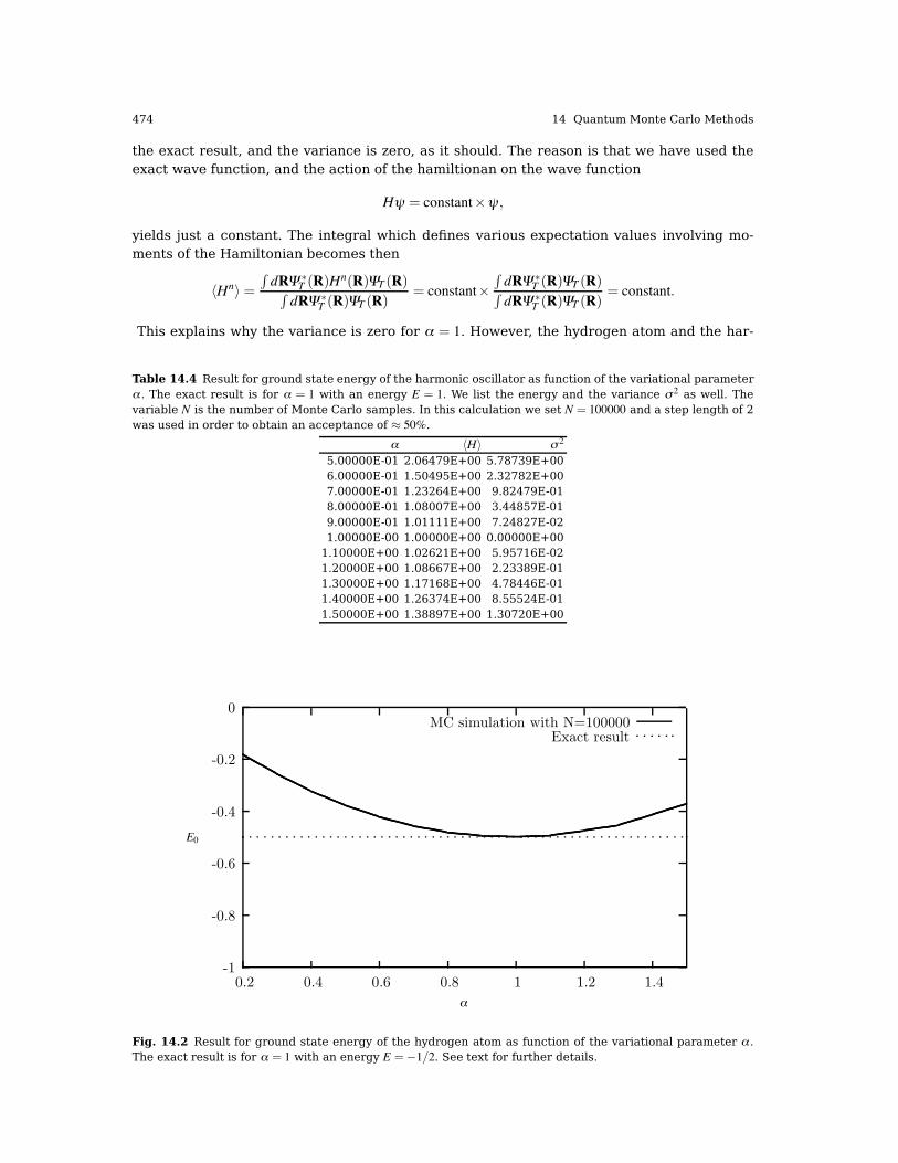
oscillator and the hydrogen atom, respectively, as functions of the variational parameter α.These results are also displayed in Tables 14.4 and 14.5. In these tables we list the varianceand the standard deviation as well. We note that at α = 1 for the hydrogen atom, we obtain
474 14 Quantum Monte Carlo Methods
the exact result, and the variance is zero, as it should. The reason is that we have used theexact wave function, and the action of the hamiltionan on the wave function
Hψ = constant$ψ ,
yields just a constant. The integral which defines various expectation values involving mo-ments of the Hamiltonian becomes then
!Hn"="dRΨ#T (R)Hn(R)ΨT (R)"
dRΨ#T (R)ΨT (R)= constant$
"dRΨ#T (R)ΨT (R)"dRΨ#T (R)ΨT (R)
= constant.
This explains why the variance is zero for α = 1. However, the hydrogen atom and the har-
Table 14.4 Result for ground state energy of the harmonic oscillator as function of the variational parameterα . The exact result is for α = 1 with an energy E = 1. We list the energy and the variance σ 2 as well. Thevariable N is the number of Monte Carlo samples. In this calculation we set N = 100000 and a step length of 2was used in order to obtain an acceptance of - 50%.
α !H" σ 2
5.00000E-01 2.06479E+00 5.78739E+006.00000E-01 1.50495E+00 2.32782E+007.00000E-01 1.23264E+00 9.82479E-018.00000E-01 1.08007E+00 3.44857E-019.00000E-01 1.01111E+00 7.24827E-021.00000E-00 1.00000E+00 0.00000E+001.10000E+00 1.02621E+00 5.95716E-021.20000E+00 1.08667E+00 2.23389E-011.30000E+00 1.17168E+00 4.78446E-011.40000E+00 1.26374E+00 8.55524E-011.50000E+00 1.38897E+00 1.30720E+00
-1
-0.8
-0.6
-0.4
-0.2
0
0.2 0.4 0.6 0.8 1 1.2 1.4
E0
α
MC simulation with N=100000Exact result
Fig. 14.2 Result for ground state energy of the hydrogen atom as function of the variational parameter α .The exact result is for α = 1 with an energy E =%1/2. See text for further details.
14.5 Variational Monte Carlo for atoms 475
monic oscillator are some of the few cases where we can use a trial wave function proportionalto the exact one. These two systems offer some of the few examples where we can find anexact solution to the problem. In most cases of interest, we do not know a priori the exact
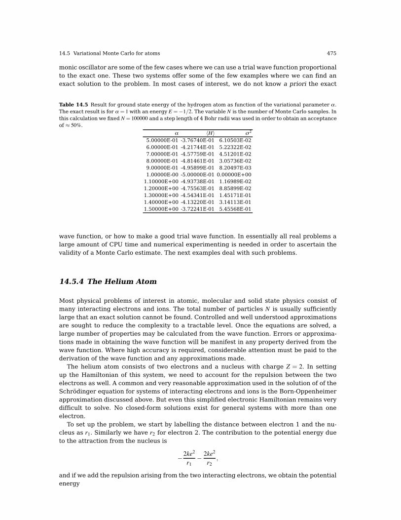
Table 14.5 Result for ground state energy of the hydrogen atom as function of the variational parameter α .The exact result is for α = 1 with an energy E =%1/2. The variable N is the number of Monte Carlo samples. Inthis calculation we fixed N = 100000 and a step length of 4 Bohr radii was used in order to obtain an acceptanceof - 50%.
α !H" σ 2
5.00000E-01 -3.76740E-01 6.10503E-026.00000E-01 -4.21744E-01 5.22322E-027.00000E-01 -4.57759E-01 4.51201E-028.00000E-01 -4.81461E-01 3.05736E-029.00000E-01 -4.95899E-01 8.20497E-031.00000E-00 -5.00000E-01 0.00000E+001.10000E+00 -4.93738E-01 1.16989E-021.20000E+00 -4.75563E-01 8.85899E-021.30000E+00 -4.54341E-01 1.45171E-011.40000E+00 -4.13220E-01 3.14113E-011.50000E+00 -3.72241E-01 5.45568E-01
wave function, or how to make a good trial wave function. In essentially all real problems alarge amount of CPU time and numerical experimenting is needed in order to ascertain thevalidity of a Monte Carlo estimate. The next examples deal with such problems.
14.5.4 The Helium Atom
Most physical problems of interest in atomic, molecular and solid state physics consist ofmany interacting electrons and ions. The total number of particles N is usually sufficientlylarge that an exact solution cannot be found. Controlled and well understood approximationsare sought to reduce the complexity to a tractable level. Once the equations are solved, alarge number of properties may be calculated from the wave function. Errors or approxima-tions made in obtaining the wave function will be manifest in any property derived from thewave function. Where high accuracy is required, considerable attention must be paid to thederivation of the wave function and any approximations made.
The helium atom consists of two electrons and a nucleus with charge Z = 2. In settingup the Hamiltonian of this system, we need to account for the repulsion between the twoelectrons as well. A common and very reasonable approximation used in the solution of of theSchrödinger equation for systems of interacting electrons and ions is the Born-Oppenheimerapproximation discussed above. But even this simplified electronic Hamiltonian remains verydifficult to solve. No closed-form solutions exist for general systems with more than oneelectron.
To set up the problem, we start by labelling the distance between electron 1 and the nu-cleus as r1. Similarly we have r2 for electron 2. The contribution to the potential energy dueto the attraction from the nucleus is
%2ke2
r1%
2ke2
r2,
and if we add the repulsion arising from the two interacting electrons, we obtain the potentialenergy
476 14 Quantum Monte Carlo Methods
V (r1,r2) =%2ke2
r1%
2ke2
r2+ke2
r12,
with the electrons separated at a distance r12 = |r1% r2|. The Hamiltonian becomes then
!H=% h2∇21
2m% h2∇2
22m%
2ke2
r1%
2ke2
r2+ke2
r12,
and Schrödingers equation reads!Hψ = Eψ .
Note that this equation has been written in atomic units (a.u.) which are more convenientfor quantum mechanical problems. This means that the final energy has to be multiplied by a2$E0, where E0 = 13.6 eV, the binding energy of the hydrogen atom.
A very simple first approximation to this system is to omit the repulsion between the twoelectrons. The potential energy becomes then
V (r1,r2)-%Zke2
r1%Zke2
r2.
The advantage of this approximation is that each electron can be treated as being indepen-dent of each other, implying that each electron sees just a central symmetric potential, orcentral field.
To see whether this gives a meaningful result, we set Z = 2 and neglect totally the repulsionbetween the two electrons. Electron 1 has the following Hamiltonian
!h1 =% h2∇2
12m%
2ke2
r1,
with pertinent wave function and eigenvalue Ea
!h1ψa = Eaψa,
where a = {nalamla} are the relevant quantum numbers needed to describe the system. Weassume here that we can use the hydrogen-like solutions, but with Z not necessarily equal toone. The energy Ea is
Ea =%Z2E0n2a
.
In a similar way, we obtain for electron 2
!h2 =% h2∇2
22m%
2ke2
r2,
with wave function ψb, b= {nblbmlb} and energy
Eb =Z2E0
n2b
.
Since the electrons do not interact, the ground state wave function of the helium atom isgiven by
ψ = ψaψb,
resulting in the following approximation to Schrödinger’s equation+!h1 +!h2
,ψ =
+!h1 +!h2
,ψa(r1)ψb(r2) = Eabψa(r1)ψb(r2).

14.5 Variational Monte Carlo for atoms 477
The energy becomes then+!h1ψa(r1)
,ψb(r2)+
+!h2ψb(r2)
,ψa(r1) = (Ea+Eb)ψa(r1)ψb(r2),
yielding
Eab = Z2E0
#1n2a+
1n2b
$.
If we insert Z = 2 and assume that the ground state is determined by two electrons in thelowest-lying hydrogen orbit with na = nb = 1, the energy becomes
Eab = 8E0 =%108.8 eV,
while the experimental value is %78.8 eV. Clearly, this discrepancy is essentially due to ouromission of the repulsion arising from the interaction of two electrons.
14.5.4.1 Choice of trial wave function
The choice of trial wave function is critical in variational Monte Carlo calculations. How tochoose it is however a highly non-trivial task. All observables are evaluated with respect tothe probability distribution
P(R) = |ψT (R)|2"|ψT (R)|2 dR
.
generated by the trial wave function. The trial wave function must approximate an exacteigenstate in order that accurate results are to be obtained. Improved trial wave functionsalso improve the importance sampling, reducing the cost of obtaining a certain statisticalaccuracy.
Quantum Monte Carlo methods are able to exploit trial wave functions of arbitrary forms.Any wave function that is physical and for which the value, the gradient and the laplacian ofthe wave function may be efficiently computed can be used. The power of Quantum MonteCarlo methods lies in the flexibility of the form of the trial wave function.
It is important that the trial wave function satisfies as many known properties of the exactwave function as possible. A good trial wave function should exhibit much of the same fea-tures as does the exact wave function. Especially, it should be well-defined at the origin, thatis Ψ (|R| = 0) 0= 0, and its derivative at the origin should also be well-defined . One possibleguideline in choosing the trial wave function is the use of constraints about the behavior ofthe wave function when the distance between one electron and the nucleus or two electronsapproaches zero. These constraints are the so-called “cusp conditions” and are related to thederivatives of the wave function.
To see this, let us single out one of the electrons in the helium atom and assume that thiselectron is close to the nucleus, i.e., r1 . 0. We assume also that the two electrons are farfrom each other and that r2 0= 0. The local energy can then be written as
EL(R) =1
ψT (R)HψT (R) =
1ψT (R)
#%
12∇2
1%Zr1
$ψT (R)+finite terms.
Writing out the kinetic energy term in the spherical coordinates of electron 1, we arrive atthe following expression for the local energy
EL(R) =1
RT (r1)
#%
12d2
dr21%
1r1
ddr1%Zr1
$RT (r1)+finite terms,

478 14 Quantum Monte Carlo Methods
where RT (r1) is the radial part of the wave function for electron 1. We have also used that theorbital momentum of electron 1 is l = 0. For small values of r1, the terms which dominate are
limr1.0
EL(R) =1
RT (r1)
#%
1r1
ddr1%Zr1
$RT (r1),
since the second derivative does not diverge due to the finiteness ofΨ at the origin. The latterimplies that in order for the kinetic energy term to balance the divergence in the potentialterm, we must have
1RT (r1)
dRT (r1)
dr1=%Z,
implying thatRT (r1) ∝ e%Zr1 .
A similar condition applies to electron 2 as well. For orbital momenta l> 0 it is rather straight-forward to show that
1RT (r)
dRT (r)dr
=%Z
l+ 1.
Another constraint on the wave function is found when the two electrons are approachingeach other. In this case it is the dependence on the separation r12 between the two electronswhich has to reflect the correct behavior in the limit r12 . 0. The resulting radial equationfor the r12 dependence is the same for the electron-nucleus case, except that the attractiveCoulomb interaction between the nucleus and the electron is replaced by a repulsive interac-tion and the kinetic energy term is twice as large.
To find an ansatz for the correlated part of the wave function, it is useful to rewrite thetwo-particle local energy in terms of the relative and center-of-mass motion. Let us denotethe distance between the two electrons as r12. We omit the center-of-mass motion since weare only interested in the case when r12. 0. The contribution from the center-of-mass (CoM)variable RCoM gives only a finite contribution. We focus only on the terms that are relevantfor r12. The relevant local energy becomes then
limr12.0
EL(R) =1
RT (r12)
&
2 d2
dr2i j+
4ri j
ddri j
+2ri j%l(l+ 1)r2i j
+ 2E
'
RT (r12) = 0,
where l is now equal 0 if the spins of the two electrons are anti-parallel and 1 if they areparallel. Repeating the argument for the electron-nucleus cusp with the factorization of theleading r-dependency, we get the similar cusp condition:
dRT (r12)
dr12=%
12(l+ 1)
RT (r12) r12. 0
resulting in
RT ∝
-.
/
exp(ri j/2) for anti-parallel spins, l = 0
exp(ri j/4) for parallel spins, l = 1.
This is so-called cusp condition for the relative motion, resulting in a minimal requirementfor the correlation part of the wave fuction. For general systems containing more than twoelectrons, we have this condition for each electron pair i j.
Based on these consideration, a possible trial wave function which ignores the ’cusp’-condition between the two electrons is
ψT (R) = e%α(r1+r2), (14.21)

14.5 Variational Monte Carlo for atoms 479
where r1,2 are dimensionless radii and α is a variational parameter which is to be interpretedas an effective charge.
A possible trial wave function which also reflects the ’cusp’-condition between the twoelectrons is
ψT (R) = e%α(r1+r2)er12/2. (14.22)
The last equation can be generalized to
ψT (R) = φ(r1)φ(r2) . . .φ(rN)∏i< j
f (ri j),
for a system with N electrons or particles. The wave function φ(ri) is the single-particle wavefunction for particle i, while f (ri j) account for more complicated two-body correlations. Forthe helium atom, we placed both electrons in the hydrogenic orbit 1s. We know that theground state for the helium atom has a symmetric spatial part, while the spin wave functionis anti-symmetric in order to obey the Pauli principle. In the present case we need not to dealwith spin degrees of freedom, since we are mainly trying to reproduce the ground state ofthe system. However, adopting such a single-particle representation for the individual elec-trons means that for atoms beyond the ground state of helium, we cannot continue to placeelectrons in the lowest hydrogenic orbit. This is a consenquence of the Pauli principle, whichstates that the total wave function for a system of identical particles such as fermions, has tobe anti-symmetric. One way to account for this is by introducing the so-called Slater deter-minant (to be discussed in more detail in chapter 15). This determinant is written in terms ofthe various single-particle wave functions.
If we consider the helium atom with two electrons in the 1s state, we can write the totalSlater determinant as
Φ(r1,r2,α,β ) =1+2
0000ψα(r1) ψα(r2)ψβ (r1) ψβ (r2)
0000 ,
with α = nlmlsms = (1001/21/2) and β = nlmlsms = (1001/2% 1/2) or using ms = 1/2 =1 andms = %1/2 =2 as α = nlmlsms = (1001/2 1) and β = nlmlsms = (1001/2 2). It is normal to skipthe two quantum numbers sms of the one-electron spin. We introduce therefore the shorthandnlml 1 or nlml 2) for a particular state where an arrow pointing upward represents ms = 1/2and a downward arrow stands for ms =%1/2. Writing out the Slater determinant
Φ(r1,r2,α,β ) =1+21ψα(r1)ψβ (r2)%ψβ (r1)ψγ (r2)
2,
we see that the Slater determinant is antisymmetric with respect to the permutation of twoparticles, that is
Φ(r1,r2,α,β ) =%Φ(r2,r1,α,β ).
The Slater determinant obeys the cusp condition for the two electrons and combined withthe correlation part we could write the ansatz for the wave function as
ψT (R) =1+21ψα(r1)ψβ (r2)%ψβ (r1)ψγ(r2)
2f (r12),
Several forms of the correlation function f (ri j) exist in the literature and we will mentiononly a selected few to give the general idea of how they are constructed. A form given byHylleraas that had great success for the helium atom was the series expansion
f (ri j) = exp(εs)∑kckrlk smk tnk

480 14 Quantum Monte Carlo Methods
where the inter-particle separation ri j for simplicity is written as r. In addition s = ri+ ri andt = ri% ri with ri and r j being the two electron-nucleus distances. All the other quantities arefree parameters. Notice that the cusp condition is satisfied by the exponential. Unfortunatelythe convergence of this function turned out to be quite slow. For example, to pinpoint the He-energy to the fourth decimal digit a nine term function would suffice. To double the numberof digits, one needed almost 1100 terms.
The so called Padé-Jastrow form, however, is more suited for larger systems. It is based onan exponential function with a rational exponent:
f (ri j) = exp(U)
In its general form,U is a potential series expansion on both the absolute particle coordinatesri and the inter-particle coordinates ri j:
U =N
∑i< j
3
45∑kαk r
ki
1+∑kα )kr
ki
6
78+N
∑i
3
45∑kβk r
ki j
1+∑kβ )kr
ki j
6
78
A typical Padé-Jastrow function used for quantum mechanical Monte Carlo calculations ofmolecular and atomic systems is
exp#
ari j(1+β ri j)
$
where β is a variational parameter and a dependes on the spins of the interacting particles.
14.5.5 Program Example for Atomic Systems
The variational Monte Carlo algorithm consists of two distinct parts. In the first a walker, asingle electron in our case, consisting of an initially random set of electron positions is prop-agated according to the Metropolis algorithm, in order to equilibrate it and begin sampling .In the second part, the walker continues to be moved, but energies and other observables arealso accumulated for later averaging and statistical analysis. In the program below, the elec-trons are moved individually and not as a whole configuration. This improves the efficiency ofthe algorithm in larger systems, where configuration moves require increasingly small stepsto maintain the acceptance ratio. The main part of the code contains calls to various func-tions, setup and declarations of arrays etc. Note that we have defined a fixed step length hfor the numerical computation of the second derivative of the kinetic energy. Furthermore,we perform the Metropolis test when we have moved all electrons. This should be comparedto the case where we move one electron at the time and perform the Metropolis test. The lat-ter is similar to the algorithm for the Ising model discussed in the previous chapter. A moredetailed discussion and better statistical treatments and analyses are discussed in chapters17 and 15.
http://folk.uio.no/compphys/programs/chapter14/cpp/program1.cpp
// Variational Monte Carlo for atoms with up to two electrons
#include <iostream>#include <fstream>#include <iomanip>#include "lib.h"
using namespace std;// output file as global variable
ofstream ofile;

14.5 Variational Monte Carlo for atoms 481
Initialize:Set rold, α
andΨT%α(rold)
Suggesta move
Computeacceptanceratio R
Generate auniformlydistributedvariable r
IsR( r?
Reject move:rnew = rold
Accept move:rold = rnew
Lastmove?
Get localenergy EL
LastMCstep?
Collectsamples
End
yes
no
yes
yes
no
Fig. 14.3 Chart flow for the Quantum Varitional Monte Carlo algorithm.

482 14 Quantum Monte Carlo Methods
// the step length and its squared inverse for the second derivative
#define h 0.001
#define h2 1000000
// declaraton of functions
// Function to read in data from screen, note call by reference
void initialise(int&, int&, int&, int&, int&, int&, double&) ;
// The Mc sampling for the variational Monte Carlo
void mc_sampling(int, int, int, int, int, int, double, double *, double *);
// The variational wave function
double wave_function(double **, double, int, int);
// The local energy
double local_energy(double **, double, double, int, int, int);
// prints to screen the results of the calculations
void output(int, int, int, double *, double *);
// Begin of main program
//int main()
int main(int argc, char* argv[]){char *outfilename;int number_cycles, max_variations, thermalization, charge;int dimension, number_particles;double step_length;
double *cumulative_e, *cumulative_e2;
// Read in output file, abort if there are too few command-line arguments
if( argc <= 1 ){cout << "Bad Usage: " << argv[0] <<
" read also output file on same line" << endl;exit(1);
}else{outfilename=argv[1];
}
ofile.open(outfilename);// Read in data
initialise(dimension, number_particles, charge,max_variations, number_cycles,
thermalization, step_length) ;cumulative_e = new double[max_variations+1];
cumulative_e2 = new double[max_variations+1];
// Do the mc sampling
mc_sampling(dimension, number_particles, charge,max_variations, thermalization,
number_cycles, step_length, cumulative_e, cumulative_e2);
// Print out results
output(max_variations, number_cycles, charge, cumulative_e, cumulative_e2);delete [] cumulative_e; delete [] cumulative_e;ofile.close(); // close output file
return 0;}

14.5 Variational Monte Carlo for atoms 483
The implementation of the brute force Metropolis algorithm is shown in the next function.Here we have a loop over the variational variables α. It calls two functions, one to computethe wave function and one to update the local energy.
// Monte Carlo sampling with the Metropolis algorithm
void mc_sampling(int dimension, int number_particles, int charge,int max_variations,
int thermalization, int number_cycles, double step_length,double *cumulative_e, double *cumulative_e2)
{int cycles, variate, accept, dim, i, j;long idum;double wfnew, wfold, alpha, energy, energy2, delta_e;
double **r_old, **r_new;alpha = 0.5*charge;idum=-1;// allocate matrices which contain the position of the particles
r_old = (double **) matrix( number_particles, dimension, sizeof(double));r_new = (double **) matrix( number_particles, dimension, sizeof(double));
for (i = 0; i < number_particles; i++) {for ( j=0; j < dimension; j++) {r_old[i][j] = r_new[i][j] = 0;
}}// loop over variational parameters
for (variate=1; variate <= max_variations; variate++){// initialisations of variational parameters and energies
alpha += 0.1;energy = energy2 = 0; accept =0; delta_e=0;// initial trial position, note calling with alpha
// and in three dimensions
for (i = 0; i < number_particles; i++) {for ( j=0; j < dimension; j++) {
r_old[i][j] = step_length*(ran1(&idum)-0.5);}
}
wfold = wave_function(r_old, alpha, dimension, number_particles);// loop over monte carlo cycles
for (cycles = 1; cycles <= number_cycles+thermalization; cycles++){// new position
for (i = 0; i < number_particles; i++) {for ( j=0; j < dimension; j++) {
r_new[i][j] = r_old[i][j]+step_length*(ran1(&idum)-0.5);}
}wfnew = wave_function(r_new, alpha, dimension, number_particles);// Metropolis test
if(ran1(&idum) <= wfnew*wfnew/wfold/wfold ) {
for (i = 0; i < number_particles; i++) {for ( j=0; j < dimension; j++) {r_old[i][j]=r_new[i][j];
}}
wfold = wfnew;accept = accept+1;
}// compute local energy
if ( cycles > thermalization ) {delta_e = local_energy(r_old, alpha, wfold, dimension,
number_particles, charge);

484 14 Quantum Monte Carlo Methods
// update energies
energy += delta_e;
energy2 += delta_e*delta_e;}
} // end of loop over MC trials
cout << "variational parameter= " << alpha<< " accepted steps= " << accept << endl;// update the energy average and its squared
cumulative_e[variate] = energy/number_cycles;cumulative_e2[variate] = energy2/number_cycles;
} // end of loop over variational steps
free_matrix((void **) r_old); // free memory
free_matrix((void **) r_new); // free memory
} // end mc_sampling function
The wave function is in turn defined in the next function. Here we limit ourselves to a functionwhich consists only of the product of single-particle wave functions.
// Function to compute the squared wave function, simplest form
double wave_function(double **r, double alpha,int dimension, int number_particles){int i, j, k;double wf, argument, r_single_particle, r_12;
argument = wf = 0;
for (i = 0; i < number_particles; i++) {r_single_particle = 0;for (j = 0; j < dimension; j++) {r_single_particle += r[i][j]*r[i][j];
}argument += sqrt(r_single_particle);
}wf = exp(-argument*alpha) ;return wf;
}
Finally, the local energy is computed using a numerical derivation for the kinetic energy. Weuse the familiar expression derived in Eq. (3.4), that is
f ))0 =fh% 2 f0 + f%h
h2 ,
in order to compute
%1
2ψT (R)∇2ψT (R). (14.23)
The variable h is a chosen step length. For helium, since it is rather easy to evaluate thelocal energy, the above is an unnecessary complication. However, for many-electron or othermany-particle systems, the derivation of a closed-form expression for the kinetic energy canbe quite involved, and the numerical evaluation of the kinetic energy using Eq. (3.4) mayresult in a simpler code and/or even a faster one.
// Function to calculate the local energy with num derivative
double local_energy(double **r, double alpha, double wfold, int dimension,int number_particles, int charge)
{int i, j , k;double e_local, wfminus, wfplus, e_kinetic, e_potential, r_12,

14.5 Variational Monte Carlo for atoms 485
r_single_particle;double **r_plus, **r_minus;
// allocate matrices which contain the position of the particles
// the function matrix is defined in the progam library
r_plus = (double **) matrix( number_particles, dimension, sizeof(double));r_minus = (double **) matrix( number_particles, dimension, sizeof(double));for (i = 0; i < number_particles; i++) {
for ( j=0; j < dimension; j++) {r_plus[i][j] = r_minus[i][j] = r[i][j];
}}// compute the kinetic energy
e_kinetic = 0;for (i = 0; i < number_particles; i++) {for (j = 0; j < dimension; j++) {r_plus[i][j] = r[i][j]+h;r_minus[i][j] = r[i][j]-h;wfminus = wave_function(r_minus, alpha, dimension, number_particles);
wfplus = wave_function(r_plus, alpha, dimension, number_particles);e_kinetic -= (wfminus+wfplus-2*wfold);r_plus[i][j] = r[i][j];r_minus[i][j] = r[i][j];
}}
// include electron mass and hbar squared and divide by wave function
e_kinetic = 0.5*h2*e_kinetic/wfold;// compute the potential energy
e_potential = 0;// contribution from electron-proton potential
for (i = 0; i < number_particles; i++) {
r_single_particle = 0;for (j = 0; j < dimension; j++) {r_single_particle += r[i][j]*r[i][j];
}e_potential -= charge/sqrt(r_single_particle);
}// contribution from electron-electron potential
for (i = 0; i < number_particles-1; i++) {for (j = i+1; j < number_particles; j++) {r_12 = 0;for (k = 0; k < dimension; k++) {
r_12 += (r[i][k]-r[j][k])*(r[i][k]-r[j][k]);}e_potential += 1/sqrt(r_12);
}}free_matrix((void **) r_plus); // free memory
free_matrix((void **) r_minus);e_local = e_potential+e_kinetic;return e_local;
}
The remaining part of the program consists of the output and initialize functions and is notlisted here.
The way we have rewritten Schrödinger’s equation results in energies given in atomicunits. If we wish to convert these energies into more familiar units like electronvolt (eV), wehave to multiply our reults with 2E0 where E0 = 13.6 eV, the binding energy of the hydrogenatom. Using Eq. (14.21) for the trial wave function, we obtain an energy minimum at α =

486 14 Quantum Monte Carlo Methods
1.68754. The ground state is E = %2.85 in atomic units or E = %77.5 eV. The experimentalvalue is %78.8 eV. Obviously, improvements to the wave function such as including the ’cusp’-condition for the two electrons as well, see Eq. (14.22), could improve our agreement withexperiment.
We note that the effective charge is less than the charge of the nucleus. We can interpretthis reduction as an effective way of incorporating the repulsive electron-electron interaction.Finally, since we do not have the exact wave function, we see from Fig. 14.4 that the varianceis not zero at the energy minimum. Techniques such as importance sampling, to be contrasted
-3
-2.9
-2.8
-2.7
-2.6
-2.5
-2.4
1 1.2 1.4 1.6 1.8 2
E0
α
MC simulation with N=107
Exact result
Fig. 14.4 Result for ground state energy of the helium atom using Eq. (14.21) for the trial wave function.A total of 107 Monte Carlo moves were used with a step length of 1 Bohr radius. Approximately 50% of allproposed moves were accepted. The variance at the minimum is 1.026, reflecting the fact that we do not havethe exact wave function. The variance has a minimum at value of α different from the energy minimum. Thenumerical results are compared with the exact result E[Z] = Z2%4Z+ 5
8Z.
to the brute force Metropolis sampling used here, and various optimization techniques of thevariance and the energy, will be discussed in the next section and in chapter 17.
14.5.6 Importance sampling
As mentioned in connection with the generation of random numbers, sequential correlationsmust be given thorough attention as it may lead to bad error estimates of our numericalresults.
There are several things we need to keep in mind in order to keep the correlation low. Firstof all, the transition acceptance must be kept as high as possible. Otherwise, a walker willdwell at the same spot in state space for several iterations at a time, which will clearly leadto high correlation between nearby succeeding measurements.
4 With hydrogen like wave functions for the 1s state one can easily calculate the energy of the ground statefor the helium atom as function of the charge Z. The results is E[Z] = Z2% 4Z+ 5
8Z, and taking the derivativewith respect to Z to find the minumum we get Z = 2% 5
16 = 1.6875. This number represents an optimal effectivecharge.

14.5 Variational Monte Carlo for atoms 487
Secondly, when using the simple symmetric form of ω(rold, rnew), one has to keep in mindthe random walk nature of the algorithm. Transitions will be made between points that arerelatively close to each other in state space, which also clearly contributes to increase corre-lation. The seemingly obvious way to deal with this would be just to increase the step size, al-lowing the walkers to cover more of the state space in fewer steps (thus requiring fewer stepsto reach ergodicity). But unfortunately, long before the step length becomes desirably large,the algorithm breaks down. When proposing moves symmetrically and uniformly around rold,the step acceptance becomes directly dependent on the step length in such a way that a toolarge step length reduces the acceptance. The reason for this is very simple. As the steplength increases, a walker will more likely be given a move proposition to areas of very lowprobability, particularly if the governing trial wave function describes a localized system. Ineffect, the effective movement of the walkers again becomes too small, resulting in largecorrelation. For optimal results we therefore have to balance the step length with the accep-tance.
With a transition suggestion rule ω as simple as the uniform symmetrical one emphasizedso far, the usual rule of thumb is to keep the acceptance around 0.5. But the optimal intervalvaries a lot from case to case. We therefore have to treat each numerical experiment withcare.
By choosing a better ω, we can still improve the efficiency of the step length versus accep-tance. Recall that ω may be chosen arbitrarily as long as it fulfills ergodicity, meaning that ithas to allow the walker to reach any point of the state space in a finite number of steps. Whatwe basically want is an ω that pushes the ratio towards unity, increasing the acceptance. Thetheoretical situation of ω exactly equal to p itself:
ω(rnew, rold) = ω(rnew) = p(rnew)
would give the maximal acceptance of 1. But then we would already have solved the prob-lem of producing points distributed according to p. One typically settles on modifying thesymmetrical ω so that the walkers move more towards areas of the state space where thedistribution is large. One such procedure is the Fokker-Planck formalism where the walkersare moved according to the gradient of the distribution. The formalism “pushes” the walkersin a “desirable” direction. The idea is to propose moves similarly to an isotropic diffusionprocess with a drift. A new position xnew is calculated from the old one, xold, as follows:
rnew = rold+ χ+DF(rold)δ t (14.24)
Here χ is a Gaussian pseudo-random number with mean equal zero and variance equal 2Dδ t.It accounts for the diffusion part of the transition. The third term on the left hand side ac-counts for the drift. F is a drift velocity dependent on the position of the walker and is derivedfrom the quantum mechanical wave function ψ. The constant D, being the diffusion constantof χ , also adjusts the size of the drift. δ t is a time step parameter whose presence will beclarified shortly.
It can be shown that the ω corresponding to the move proposition rule in Eq. (14.24)becomes (in non-normalized form):
ω(rold, rnew) = exp#%(rnew% rold%Dδ tF(rold))2
4Dδ t
$(14.25)
which, as expected, is a Gaussian with variance 2Dδ t centered slightly off rold due to the driftterm DF(rold)δ t.
What is the optimal choice for the drift term? From statistical mechanics we know that asimple isotropic drift diffusion process obeys a Fokker-Planck equation of the form:

488 14 Quantum Monte Carlo Methods
∂ f∂ t
=∑iD∂∂xi
#∂∂xi%Fi(F)
$f (14.26)
where f is the continuous distribution of walkers. Equation (14.24) is a discretized realizationof such a process where δ t is the discretized time step. In order for the solution f to convergeto the desired distribution p, it can be shown that the drift velocity has to be chosen as follows:
F =1f∇ f
where the operator ∇ is the vector of first derivatives of all spatial coordinates. Convergencefor such a diffusion process is only guaranteed when the time step approaches zero. But in theMetropolis algorithm, where drift diffusion is used just as a transition proposition rule, thisbias is corrected automatically by the rejection mechanism. In our application, the desiredprobability distribution function being the square absolute of the wave function, f = |ψ |2, thedrift velocity becomes:
F = 2 1ψ∇ψ (14.27)
As expected, the walker is “pushed” along the gradient of the wave function.When dealing with many-particle systems, we should also consider whether to move only
one particle at a time at each transition or all at once. The former method may often be moreefficient. A movement of only one particle will restrict the accessible space a walker can moveto in a single transition even more, thus introducing correlation. But on the other hand, theacceptance is increased so that each particle can be moved further than it could in a standardall-particle move. It is also computationally far more efficient to do one-particle transitionsparticularly when dealing with complicated distributions governing many-dimensional anti-symmetrical fermionic systems.
Alternatively, we can treat the sequence of all one-particle transitions as one total transi-tion of all particles. This gives a larger effective step length thus reducing the correlation.From a computational point of view, we may not gain any speed by summing up the individualone-particle transitions as opposed to doing an all-particle transition. But the reduced corre-lation increases the total efficiency. We are able to do fewer calculations in order to reach thesame numerical accuracy.
Another way to acquire some control over the correlation is to do a so called blockingprocedure on our set of numerical measurements. This is discussed in chapter 16.
14.6 Exercises
14.1. The aim of this problem is to test the variational Monte Carlo apppled to light atoms.We will test different trial wave function ΨT . The systems we study are atoms consisting oftwo electrons only, such as the helium atom, LiII and BeIII . The atom LiII has two electronsand Z = 3 while BeIII has Z = 4 but still two electrons only. A general ansatz for the trial wavefunction is
ψT (R) = φ(r1)φ(r2) f (r12). (14.28)
For all systems we assume that the one-electron wave functions φ(ri) are described by the anelecron in the lowest hydrogen orbital 1s.
The specific trial functions we study are
ψT1(r1,r2,r12) = exp(%α(r1 + r2)), (14.29)

14.6 Exercises 489
where α is the variational parameter,
ψT2(r1,r2,r12) = exp(%α(r1 + r2))(1+β r12), (14.30)
with β as a new variational parameter and
ψT3(r1,r2,r12) = exp(%α(r1 + r2))exp#
r122(1+β r12)
$. (14.31)
a) Find the closed-form expressions for the local energy for the above trial wave function for thehelium atom. Study the behavior of the local energy with these functions in the limits r1. 0,r2. 0 and r12. 0.
b) Compute
!!H"="dRΨ#T (R)!H(R)ΨT (R)"dRΨ#T (R)ΨT (R)
, (14.32)
for the helium atom using the variational Monte Carlo method employing the Metropolisalgorithm to sample the different states using the trial wave function ψT1(r1,r2,r12). Compareyour results with the closed-form expression
!!H"= h2
meα2%
2732
e2
πε0α. (14.33)
c) Use the optimal value of α from the previous point to compute the ground state of the heliumatom using the other two trial wave functions ψT2(r1,r2,r12) and ψT3(r1,r2,r12). In this caseyou have to vary both α and β . Explain briefly which function ψT1(r1,r2,r12), ψT2(r1,r2,r12)and ψT3(r1,r2,r12) is the best.
d) Use the optimal value for all parameters and all wave functions to compute the expectationvalue of the mean distance !r12" between the two electrons. Comment your results.
e) We will now repeat point 1c), but we replace the helium atom with the ions LiII and BeIII .Perform first a variational calculation using the first ansatz for the trial wave functionψT1(r1,r2,r12) in order to find an optimal value for α. Use then this value to start the varia-tional calculation of the energy for the wave functions ψT2(r1,r2,r12) and ψT3(r1,r2,r12). Com-ment your results.
14.2. The H+2 molecule consists of two protons and one electron, with binding energy EB =
%2.8 eV and an equilibrium position r0 = 0.106 nm between the two protons.We define our system through the following variables. The electron is at a distance r from
a chosen origo, one of the protons is at the distance %R/2 while the other one is placed atR/2 from origo, resulting in a distance to the electron of r%R/2 and r+R/2, respectively.
In our solution of Schrödinger’s equation for this system we are going to neglect the kineticenergies of the protons, since they are 2000 times heavier than the electron. We assumethus that their velocities are negligible compared to the velocity of the electron. In additionwe omit contributions from nuclear forces, since they act at distances of several orders ofmagnitude smaller than the equilibrium position.
We can then write Schrödinger’s equation as follows
9% h2∇2
r2me
%ke2
|r%R/2|%
ke2
|r+R/2|+ke2
R
:ψ(r,R) = Eψ(r,R), (14.34)
where the first term is the kinetic energy of the electron, the second term is the potentialenergy the electron feels from the proton at %R/2 while the third term arises from the po-tential energy contribution from the proton at R/2. The last term arises due to the repulsionbetween the two protons.
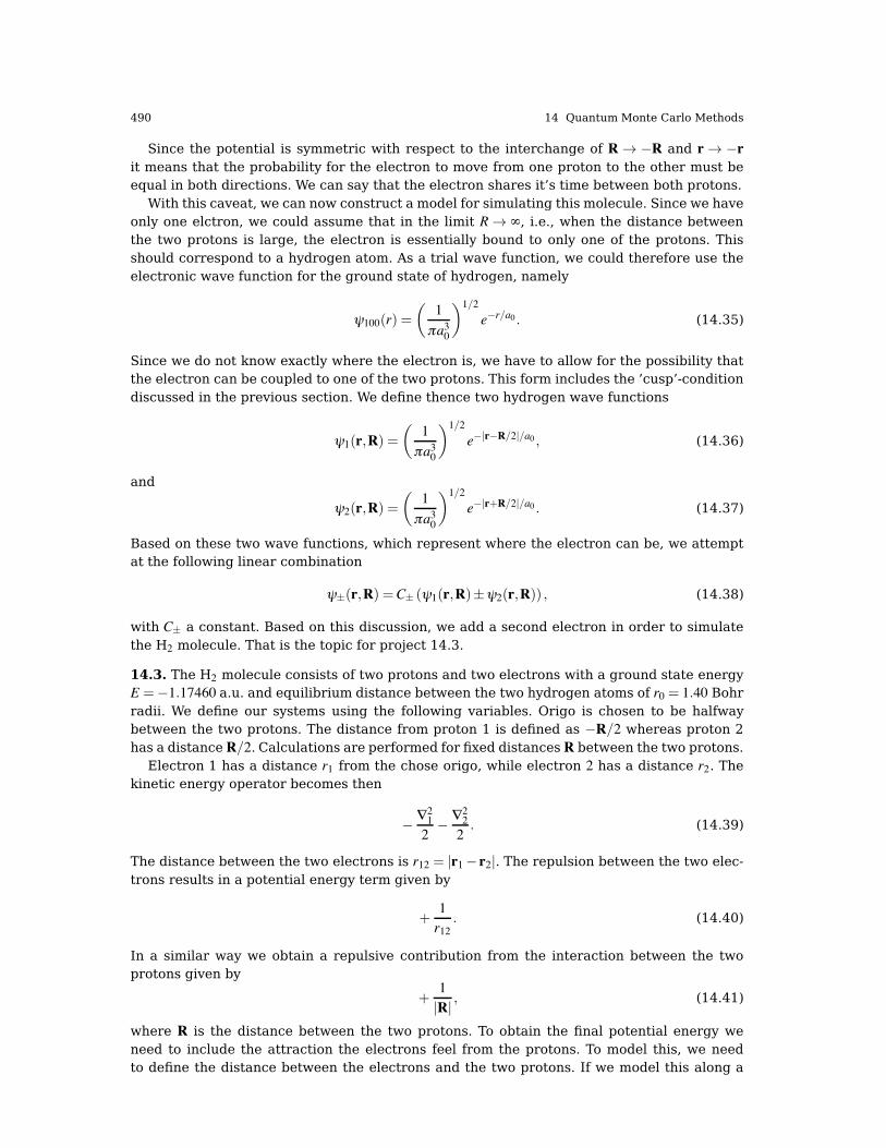
490 14 Quantum Monte Carlo Methods
Since the potential is symmetric with respect to the interchange of R.%R and r.%rit means that the probability for the electron to move from one proton to the other must beequal in both directions. We can say that the electron shares it’s time between both protons.
With this caveat, we can now construct a model for simulating this molecule. Since we haveonly one elctron, we could assume that in the limit R. ∞, i.e., when the distance betweenthe two protons is large, the electron is essentially bound to only one of the protons. Thisshould correspond to a hydrogen atom. As a trial wave function, we could therefore use theelectronic wave function for the ground state of hydrogen, namely
ψ100(r) =#
1πa3
0
$1/2e%r/a0 . (14.35)
Since we do not know exactly where the electron is, we have to allow for the possibility thatthe electron can be coupled to one of the two protons. This form includes the ’cusp’-conditiondiscussed in the previous section. We define thence two hydrogen wave functions
ψ1(r,R) =#
1πa3
0
$1/2e%|r%R/2|/a0 , (14.36)
and
ψ2(r,R) =#
1πa3
0
$1/2e%|r+R/2|/a0 . (14.37)
Based on these two wave functions, which represent where the electron can be, we attemptat the following linear combination
ψ±(r,R) =C± (ψ1(r,R)±ψ2(r,R)) , (14.38)
with C± a constant. Based on this discussion, we add a second electron in order to simulatethe H2 molecule. That is the topic for project 14.3.
14.3. The H2 molecule consists of two protons and two electrons with a ground state energyE =%1.17460 a.u. and equilibrium distance between the two hydrogen atoms of r0 = 1.40 Bohrradii. We define our systems using the following variables. Origo is chosen to be halfwaybetween the two protons. The distance from proton 1 is defined as %R/2 whereas proton 2has a distance R/2. Calculations are performed for fixed distances R between the two protons.
Electron 1 has a distance r1 from the chose origo, while electron 2 has a distance r2. Thekinetic energy operator becomes then
%∇2
12%∇2
22. (14.39)
The distance between the two electrons is r12 = |r1% r2|. The repulsion between the two elec-trons results in a potential energy term given by
+1r12
. (14.40)
In a similar way we obtain a repulsive contribution from the interaction between the twoprotons given by
+1|R| , (14.41)
where R is the distance between the two protons. To obtain the final potential energy weneed to include the attraction the electrons feel from the protons. To model this, we needto define the distance between the electrons and the two protons. If we model this along a
14.6 Exercises 491
chosen z-akse with electron 1 placed at a distance r1 from a chose origo, one proton at %R/2and the other at R/2, the distance from proton 1 to electron 1 becomes
r1p1 = r1 +R/2, (14.42)
andr1p2 = r1%R/2, (14.43)
from proton 2. Similarly, for electron 2 we obtain
r2p1 = r2 +R/2, (14.44)
andr2p2 = r2%R/2. (14.45)
These four distances define the attractive contributions to the potential energy
%1r1p1%
1r1p2%
1r2p1%
1r2p2
. (14.46)
We can then write the total Hamiltonian as
!H=%∇2
12%∇2
22%
1r1p1%
1r1p2%
1r2p1%
1r2p2
+1r12
+1|R| , (14.47)
and if we choose R= 0 we obtain the helium atom.In this project we will use a trial wave function of the form
ψT (r1,r2,R) = ψ(r1,R)ψ(r2,R)exp#
r122(1+β r12)
$, (14.48)
with the following trial wave function
ψ(r1,R) = (exp(%αr1p1)+ exp(%αr1p2)) , (14.49)
for electron 1 andψ(r2,R) = (exp(%αr2p1)+ exp(%αr2p2)) . (14.50)
The variational parameters are α and β .One can show that in the limit where all distances approach zero that
α = 1+ exp(%R/α), (14.51)
resulting in β kas the only variational parameter. The last equation is a non-linear equationwhich we can solve with for example Newton’s method discussed in chapter 4.
1. Find the local energy as function of R.2. Set up and algorithm and write a program which computes the expectation value of !!H"
using the variational Monte Carlo method with a brute force Metropolis sampling. For eachinter-proton distance R you must find the parameter β which minimizes the energy. Plot thecorresponding energy as function of the distance R between the protons.
3. Use thereafter the optimal parameter sets to compute the average distance !r12" between theelectrons where the energy as function of R exhibits its minimum. Comment your results.
4. We modify now the approximation for the wave functions of electrons 1 and 2 by subtractingthe two terms instead of adding up, viz
ψ(r1,R) = (exp(%αr1p1)% exp(%αr1p2)) , (14.52)

492 14 Quantum Monte Carlo Methods
for electron 1ψ(r2,R) = (exp(%αr2p1)% exp(%αr2p2)) , (14.53)
for electron 2. Mathematically, this approach is equally viable as the previous one. Repeatyour calculations from point b) and see if you can obtain an energy minimum as function ofR. Comment your results.


![Quantum Monte Carlo on geomaterials Dario Alfè [d.alfe@ucl.ac.uk] 2007 Summer School on Computational Materials Science Quantum Monte Carlo: From Minerals](https://img.pdfslide.us/doc/110x75/5697bf951a28abf838c90e05/quantum-monte-carlo-on-geomaterials-dario-alfe-dalfeuclacuk-2007-summer.jpg)