Quantum Monte Carlo:

Some Theoretical and Numerical Studies.

by

Heather Louise Gordon, B.Sc. Chern.

A Thesis

submitted to the Department of Chemistry

in partial fulfilment of the requirements

for the degree of

Master of Science

July 1983

Brock University

St. Catharines, Ontario

~ Heather Louise Gordon, 1983

Abstract

In Part I, theoretical derivations for Variational Monte Carlo

calculations are compared with results from a numerical calculation of

He; both indicate that minimization of the ratio estimate of E , denotedvar

EMC

' provides different optimal variational parameters than does

minimization of the variance of EMC

• Similar derivations for Diffusion

Monte Carlo calculations provide a theoretical justification for empirical

observations made by other workers.

In Part II, Importance sampling in prolate spheroidal coordinates

allows Monte Carlo calculations to be made of E for the vdW moleculevar

He2' using a simplifying partitioning of the Hamiltonian and both an

HF-SCF and an explicitly correlated wavefunction. Improvements are

suggested which would permit the extension of the computational precision

to the point where an estimate of the interaction energy could be made~

(i)

Acknowledgements

I would like to extend my thanks and appreciation to

Dr. S. M. Rothstein, with whom it has been? pleasure to work over the

past three years.

I would also like to thank the Computer Science Department of

Brock University for the use of the VAXll/780 and "the Computer Centre for

the use of the Burroughs 6700.

Thanks also to J. Hastie for her patience in typing this

manuscript.

I also acknowledge the support of an NSERC graduate scholarship.

(Li)

Table of Contents, continued .•.

Page

E.

F.

G.

H.

I.

J.

K.

L.

M.

Importance Sampling for Hylleraas Coordinates

Precision of the Variance Estimate

Derivation of (8.19)

Derivation of (8.32) and (8.33)

Evaluation of !XA(rX)XB(rX)rlx-ldrx

Terms arising from (9.19)

Comparison of Two Ratios-+- -+-

Derivation of V.u-V.u for (11.1) and (11.2)1. 1.

Importance Sampling in Prolate Spheroidal CoordinatesI\'+for Lg HeZ

97

100

102

106

108

111

113

117

121

References

List of Tables

Table I Optimization of a One-Parameter Variational Wave­

function for 1 IS He

Table II HONDO and Monte Carlo Results (n=104) for SCF1 '+Calculation of Lg HeZ

Table III'Optimi.zation. of a One-·Parameter Correlated Wave-

f '. f I\'+"unctl.0n.,or L· He2- 1 '+ gTable IV EMC for Lg HeZ using an Explicitly Correlated

Wavefunction

List of Figures

Fig. I Prolate Spheroidal Coordinate System

Fig. II Monte Carlo Estimate EHF of Hartree-Fock Energy

~ersus Internuclear Separation R for HeZ

(iv)

125

30

71

76

78

52

74

1

I. Introduction

The Schroedinger Equation

E~ (1.1)

is exactly solvable for one-electron atoms and molecules; for many-electron

atoms and molecules, approximate methods must be employed since the

interelectronic repulsion terms r~~ in the Hamiltonian H causes the1J

Schroedinger Equation to be inseparable in any coordinate system. The

Variational Method provides an approximate solution for the ground-state

energy of a system without solving the Schroedinger Equation.

The Variational Theorem [1] states that, given a trial wavefunction

Wt which is well-behaved, normalizable and obeys the boundary conditions of

the system, then

E ~ Eo var (1.2)

where E is the lowest eigenvalue of Hand E is the so-calledo var

variational energy. As the trial wavefunction more closely approximates

the true exact wavefunction, W , the variational energy approaches E •o 0

Thus the variational integral (1.2) provides an upper bound for E .o

2

The mathematical form that 1J; can assume varies widely: a compact,t

physically meaningful wavefunction may give rise to intractable integrals

while one which tries to avoid such difficulties may need so many terms

and parameters that all physical meaning is lost. An example of the

former is an explicitly correlated wavefunction, so-called because it

involves expansions in terms of the interelectronic coordinates. The

presence of such terms efficiently incorporates the effect of electron

correlation into the energy calculation but leads to very complicated

integrals. Monte Carlo techniques for integration [2-5] can be used to

numerically evaluate such integrals: the mean and variance of integrand

values evaluated at a large number of representative points over the

coordinate domain are calculated. The mean is an estimate of the value

of the integral and the statistical variance is a measure of the precision

of the estimate.

In practice, ~ is a function of a set of adjustable parameters,t

§., which are to be optimized. In the Monte Carlo scheme, this has been

done either by minimizing the Monte Carlo estimate EMC

of Evar

(1.2) [6]

or by minimizing the variance of EMC

[7]. ~e former is justified by the

variational theorem while the latter has a statistical justification: a

smaller variance means a more precise estimate. It can be shown that for

1J; the statistical variance of the Monte Carlo energy estimate is zeroo

[7, 8].

The objective of the first part of this work is to derive

expressions in order to determine theoretically which optimization scheme

is to be pieferred given a Variational Monte Carlo calculation of Evar

3

(1.2). These results are compared with those found empirically from a

Monte Carlo simulation of a simple, known system (Helium atom). The

conclusions reached are then of use in the second part of the work, where

the more complicated system of the van der Waals He2 molecule is

considered.

For He2' Self-Consistent-Field (SCF) theory fails to predict the

existence of a shallow minimum in the intermolecular energy curve because

it neglects the effect of electron correlation [9]. Hence the use of

explicitly correlated wavefunctions promises to be of use in ab initio

calculations of the interaction energy for such rare-gas systems [7, 10,

11].

In the second part of this thesis, the following are accomplished;

(i) a Monte Carlo sampling procedure for the He2 systeiJIn is constructed;

(ii) equations are developed which enable SCF results to be combined

with Monte Carlo estimates of the effect of the inclusion of a

correlation function with the SCF wavefunction;

(iii) a computer program incorporating the above is written and different

correlation functions are examined.

6

The integral in (1.2) is also a specific example of a quantum

mechanical expectation value. Given an operator, 0, the expectation or

average value is given by

<0> (2.1)

*given a distribution function W (~)~(~)d~. Hence the E 1S thevar

expectation value of the Hamiltonian, given the normalized everywhere

non-negative, probability density p(3,S)

J\fJ -;.'~ (x) \fJ (x) dxt-- t--- --

(2.2)

(See (2.5) below.)

The Monte Carlo Method offers a numerical solution to integrals

of the type shown in (2.1) where the multidimensionality and inseparability

of the particle coordinates make the analytic evaluations intractable.

In particular, as mentioned in the introduction, this occurs when the

integrand is a function of r ...1J

If 0 does not involve any differential operators, then (2.1) can

be rearranged as

<0> (2.3)

It is shown in Appendix A that the Central Limit Theorem of probability

gives

<0>n

lim n-1I O(x.)n-+oo i=1"'-1

7

(2.4)

where (x.) are a set of points in configuration space, drawn from (2.2)."'-1

In the case where 0 does involve differential operators, (2.1) can be

written as

<0>

and hence

<0> lim n-l~ [O(x.)1/J (x.)/1/J (x.)]~ "'-1 t"'-1 t"'-1

n-+oo 1=1

(2.5)

(2.6)

Equations (2.4) and (2.6) show that the integrals in (2.3) and

(2.5) may be estimated by an average over random values of the function

o or (O~ /~ ) evaluated at n representative points x. from the continuous,t t "'-1

normalized and non-negative probability function p(~). In the limit as the

number of values included in the sum becomes infinite, the estimator

becomes exact; the Monte Carlo estimate of <0>, where n < 00 will be

designated 0MC'

In addition to calculating 0MC' it is of importance to have

some estimate of the variance of 0MC' which is associated with the

precision of the Monte Carlo estimate of <0>. In Appendix A, it is shown

that, for independent samples, confidence intervals around 0MC can be

constructed from the estimate of the variance of 0MC' v;r(O~~ the true

8

variance being var(OMC). This information allows the theoretician to

state with some degree of confidence that <0> lies within some interval

surrounding 0MC. Even if confidence levels cannot be established, as is

the case with the use of correlated samples or of samples having unknown

distributions, estimates of precision are useful, since it is desirable to

consider both accuracy and precision as indicators of a successful

"experiment" [24]. In the event that true expectation values are not known,

as is the usual case in Quantum Chemical problems, some knowledge of the

precision of estimates is especially important as accuracies cannot be

established.

The normalization condition of the probability density p(~) in the

denominator of (2.1) presents the first obstacle in the computation of

Quite often, the choice of ~ (x) precludes the analytic evaluationt ~

of the normalization constant. In order to circumvent this problem, one

of two approaches may be taken. The most common, as applied to Variational

methods, is to use the Metropolis Monte Carlo technique [13]. In this

method, the set of points x. is the result of a random walk through~1

configuration space formed by a Markov process [3]. For Metropolis

sampling, the configurations ~k and ~k+1 are not statistically independent.

The advantage of the Metropolis scheme is that it is only necessary to

evaluate ratios of p(~) for successive configurations, thus the

normalization integrals cancel out. The disadvantage is that correlation

in the sample increases the variance and hence causes slow convergence

towards the expectation value. Binder [21] points out the many

considerations necessary for good Metropolis Monte Carlo work.

9

An alternative approach is to simulate both integrals in (2.1)

using a random sample of configuration points, thus avoiding correlation

in the sample. The disadvantage of this method lies in the expense of

generating the random configuration points from the inversion of a

probability density, as compared to the acception-rejection method

employed by the Metropolis technique. However, the statistical theory for

treating such samples is well-known; the straightforward analysis of

variance is an advantage because the convergence of the Monte Carlo_1

estimate towards the true answer is slow (generally on the order of n 2,

n being the sample size), and because the true answer is not generally

mown.

This second approach, which will be designated as Variational

Monte Carlo (VMC), is used in this work. Recently a third approach

called Diffusion Monte Carlo (DMC), has been applied by several workers

[25-27]. DMC contrasts with VMC and Metropolis Monte Carlo in having the

potential to estimate E rather than Eo var It is of interest to compare

the statistics for DMC with those of VMC and a short chapter, V, is devoted

to this purpose.

10

III. Principles of Monte Carlo Evaluation of Integrals

The evaluation of multiple integrals by Monte Carlo Methods is an

extension of the one-dimensional case which will be examined for simplicity.

Consider then, the integral I:

I Jbf(x)ds

a(3.1)

where f(x) is continuous over the interval a ~ x ~ b and assume that

fsL 2 (a,b) (that is,

exists and hence I exists). Equation (3.1) can be expressed in terms of

an expectation value

I - <f/p> t1f(X)/P(X)]P(X)dXa

(3.2)

over a normalized, continuous and non-negative density function, p(x),

defined in the region a ~ x ~ b:

p(x) ~ 0, a ~ x ~ b (3.3a)

1 tP(x)dxa

(3.3b)

11

The <f/p> can be termed the expected value of a continuous random function.

The variance of f/p, Var(f/p) is defined by:

Var(f/p)

t[f(X)/p(X)]2 p (X)dX - rt1f(X)/P(X)]P(X)dx]2. (3.4)a a

The sample-mean Monte Carlo Method [19] numerically evaluates I

using (3.2) by generating n random points Xl, · · Ii' X ndistributed

according to p(x) and estimating <f/p> as the mean of the f(x.}!p(x.):1 1

In

n-II f(x.)/p(x.)i=1 1 1

(3.5)

I is an unbiased estimator and converges to the exact value I as

n --+ 00. The estimate of the variance of I is, from (3.4)

(3.6)

For a sufficiently large sample, n - (n - 1) and

(3.7)

Given that {x.} are n independent identically distributed random1

variables, then the {f(x.)/p(x.)} are likewise distributed. Hence,1 ].

and

<f(x.)/p(x.»1. 1.

I 1. 1, ... , n

12

(3.8a)

Var(f(x.)/p(x.))1. 1.

Var(l) i 1, ... , n (3.8b)

where the angular brackets denote the expected value.

The expected value of the sum of the random variates is treated as

follows:

n<I f(x.)/p(x.»i=l 1. 1.

nI <f(x.)/p(x.» nli=l 1. 1.

(3.9a)

and the variance of the sum is then

nVar(I f(x.)/p(x.))

i=l 1. 1.

nI Var(f(x.)/p(x.))i=l 1. 1.

nVar(l) (3.9b)

The Central Limit Theorem (CLT) (see Appendix A) of probability

states that such a sum of random variables is asymptotically normally

distributed with mean nl and variance nVar(l):

npeI f(x.)/p(x.)) ~ N(nI, nVar(l))

i=l 1. 1.

n -+- 00 (3.10)

and so the sample mean is also asymptotically normally distributed

p(I) ~ NCr, Var(l)) n ~ 00 (3.11)

13

The significance of this theorem is that it is possible to

construct confidence intervals about I because the normal distribution

has a known mathematical form. Hence it is possible to show that the

probability of finding the true mean within 3 standard deviations of I

is about 99.7%:

(3.12)

In particular, using Vir(I) (3.7), it can be stated that the true value_ _ 1 _

I lies within the interval I ± 3Var 2 (I) approximately 99.7% of the time

due to chance, given a sufficiently large sample.

The Monte Carlo variance (3.7) is proportional to n-1 and the_ 1 _ ... 1

standard deviation Var 2 (I) to n 2. The statistical error decreases as the

sample size increases, however the convergence is slow: in order to gain

one significant digit in the precision of I" the sample must be increased

lOO-fold. In practice, almost all Monte Garlo work employs some kind of

and/or combination of variance-reduction techniques [19,20]. Importance

sampling [28] is one such technique universally employed in all types of

Quantum Monte Carlo Methods.

Consider the case where p(x) is a uniform distribution between

a ~ x ~ b; given the constraints (3.3) then

p(x) a ~ x ~ b (3.13)

Then from (3.2) and (3.5)

I (b -- a)<f>

14

(3.14)

and the Monte Carlo estimate is

In

n~l(b -- a)I f(x.)i=l ].

(3.15)

The variance of i is

Var(l)n

Var(n-1(b -- a)I f(x.))i=1 ].

(3.16)

An estimate of Var(I)is then, from (3.7),

nn-1(b -- a)2I f2(x.) -- 12

i=l ].(3.17)

Equations (3.15) and (@.17) are the Crude Monte Carlo estimate

and variance respectively; each element in the Monte Carlo sum has an

identical weight. Since a configuration point x. is just as likely to beJ

chosen as a point xk

from the distribution in (3.13), even if

i5

f(xj

) « f(xk), a great many sample points must be taken in order for

points where f(x) is large to dominate the Monte Carlo sum. Hence the

variance of the Crude Monte Carlo estimate is large.

Importance sampling uses a suitablJ chosen p(x) so that sample

points are concentrated in areas where f(x) is large; bias is removed by

a suitable weighting scheme. Equation (3.2) shows that any suitable p(x)

complying with the constraints (3.3) will provide an estimate of I. It

can be proven [19] that the minimum variance is equal to

Var(f/p )o

and occurs when

(3.18)

p (x)o

(3.19)

In other words, if f(x) is everywhere non-negative, choosing p(x) proportional

to f(x) gives a zero variance. In reality, since (3.1) is not known,

p (x) (3.19) will not be known. However, this result shows that if p(x)o

is chosen to have a shape similar to f(x), then the ratio f/p will be

relatively constant and the variance of the estimate will be reduced. The

optimal choice of p for a particular f, given the constraints (3.3), is a

difficult analytical problem [19] and in general, is taken on -the basis

of knowledge about f and the ease of normalization.

Given an importance sampling density, p(x), it is necessary to

generate a set of random variables {x.} to use in (3.5) and (3.7).].

16

Several procedures are available [29]; the inverse transform or probability

inversion method [29, 30] is used here.

Computer-generated pseudorandom numbers (so-called because they

are not truly random but comply with statistical tests of "rando,mness U)

are drawn from standard distributions. Consider then a set of pseudorandom

numbers {P.} drawn from a univariate uniform distribution: P. represents1 1

the cumulative probability of p(x) at x = x.1

P.1

The integral in (3.20) is performed and x = x. is solved ,for, given P~.1 1

Sometimes this is a difficult problem; in other cases more efficient methods

of generating {x.} are available [29].1

The multivariate case, where p = P(Xl' ••• , X ) is somewhatr

similar; the following equations apply whether or not the variables

Xl, ••• , x are independent.r

Define reduced density functions

Pk(Xl, ... , Xk ) - J.··fP(Xl' ••• , :xr )dxk+1 ···dxr

k = 1, ..... , r-1

and conditional density functions

(3.21)

(3.22)

17

Since

r-1PI(XI)II f(x.+1 IxI,

i=l 1.~ .,- X. )

1.(3.23)

the r-dimensional random numbers can be generated by first selecting Xl

i = 2, ..• , r from r. (x.} Xl, ••• , x. 1)1. 1. 1.-

successively. There are r! ordered combinations to represent Xl, ••• , X r

and hence r! possibilities to generate the sets of random variables. For

example, if r = 2, then

{

PI (XI)r2. (X2.1 XI)

P1 (X 2 ) r 2 (X I IX 2)

(3.24)

which promises two courses of action:

(1) find Xl and then X2 conditional on Xl, or

(2) find X2 and then Xl conditional on X2.

If the variables are independent, all r! combinations are equivalent;

otherwise the combination chosen depends on the efficiency of the inversion

problems posed and on the how the variables are interdependent [29].

18

IV. Variational Monte Carlo: Theoretical Derivations and Parameter

Optimization [31]

In this chapter, formulae are derived for E and the variance ofvar

the VMC energy estimate Var(EMC ) in terms of smallness parameters, which

relate to the accuracy of W. The effect of minimizing either the E ort var

Var(EMC ) with respect to variational parameters ~ in Wt is examined.

Consider an unnormalized wavefunction, Wt • Expand ~ in terms oft

the exact (normalized) ground stat~ ¢ , and (normalized) excited states,o

~k~ with the same symmetry as ~o:

00

1/J t(4.1)

where Ak are smallness parameters [32] such that Ak --+ 0 as 1/J t --+ ¢o.

(In all equations that follow, the summation is assumed to run over all

excited states.) The variational energy E (1.2) is a quotient of twovar

expectation values:

E <H>/<S> (4.2)var

where

';~

H - 1/J t HWt (4.3)

and

'1<S - WtW t (4.4)

19

(i) _ - (i) (i)where Hand 8 are functions of R = (~l , ••• , ~N ), the i-th member

of a set of n points in the configuration space of N electrons.

Upon substituting (4.1) into (4.3) and (4.4) one obtains

E +a

(4.5)

where Eo and Ek

are the exact ground and k-th excited state energies,

respectively, and similarly,

Thus,

<8> (4.6)

Evar E +o(4.7)

the well-known result that the variational energy 1S an upper bound to Eo

and is of second order in a smallness parameter.

Assume a simple random sample of n configurations, R(i). The

(crude) VMC estimate of the quotient

n- 1 IH(R(i))

1

n-1IS(R(i))1

(4.8)

converges to E (4.7) as n ~ 00 (a "consistentH estimate is provided).var

Statisticians refer to (4.8) as a ratio estimate. It has a negligible

bias for large n [33}:

I

I

I

I

I

I

I

I

I

I

I

I

I

I

I

I

I

I

I

I

I

I

I

I

I

I

I

I

I

I

I

I

I

I

I

I

I

I

I

I

I

I

I

I

I

I

I

I

I

I

I

I

I

I

I

I

I

I

I

I

I

I

I

I

I

I

I

I

(4.11)

(4.12)

(4.9)

n-lC~ ~>'k>'~(Ek - Eo) (E~ - Eo)<<P~<Pk<P~> + 0(>' 3)) + 0(n-2).

,(4.13)

(4.10)

20

The variance of the ratio estimator (4.8) is given by [33]:

[35]). Upon substitution of (4.1) into equations like the following:

where E is given by (4.7). The distribution of (4.8) is asymptoticallyvar

normal, subject to mild conditions on the distributions of Hand S [34].

one obtains:

(One may readily obtain a biased estimate of the variance from the sample

Hence the leading terms in the expected value (4.9) and the variance (4.13)

of EMC (4@)8)are second order in, A~

Details on the derivations of (4.7) and (4.13) appear in Appendix

B.

21

III

I

I

II

I

I

III

I

I

II

I

I

II

I

I

III

I

III

I

I

II

I

I

I

II

I

III

I

I

II

I

I

III

I

III

I

I

II

I

I

I

II

I

III

I

I

II

(4.14)

(4.15)0, all m.

Hence, even if it w'e're possible

infinite sample, while the latter has a statistical justification: the

It is important to contrast (4.J) and (4.13), above, with their

Assume an infinite sample, so that the sample estimate of E andvar

In practice there are one or more adjustable parameters in ~t' say

the variance are exact. By differentiating (4.7) with respect to ~, the

~, which should be optimized. This has been done by either minimizing

EMC

for a reasonably large value of n, as for example [6], or by

minimizing the variance estimate, Var(EMC)' as for example [7]. The

former is rigorously justified by the variational theorem only for an

confidence interval for E is a minimum for the given sample.var

optimum parameter values, .§.1<, obey the following equations:

By differentiating (4.13), the true variance of EMC '

Barring the trivial case of zero Ak (for all k) and/or dAk/aSm

(for all

to optimize ~ by minimizing the true variance of EMC ' the Virial Theorem

would not be obeyed; additional scaling is required [7].

analogs for a normalized variational wavefunction

1< *"J'<k and m), it is apparent that ~ ~ ~

~t

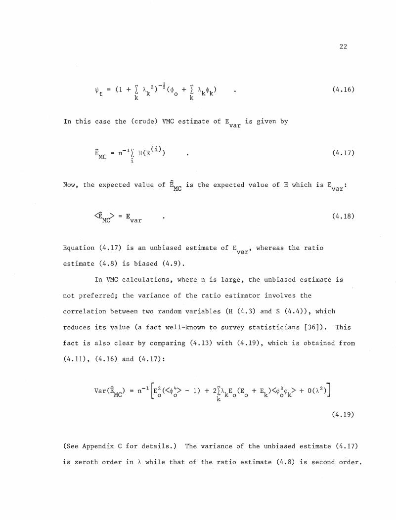
22

(4.16)

In this case the (crude) VMC estimate of E is given byvar

n-1I H(R(i))

i(4.17)

Now, the expected value of EMC is the expected value of H which is Evar

Evar (4.18)

Equation (4.17) is an unbiased estimate of E ,whereas the ratiovar

estimate (4.8) is biased (4.9).

In VMC calculations, where n is large, the unbiased estimate is

not preferred; the variance of the ratio estimator involves the

correlation between two random variables (H (4.3) and S (4.4)), which

reduces its value (a fact well-known to survey statisticians [36]). This

fact is also clear by comparing (4.13) with (4.19), which is obtained from

(4.11), (4.16) and (4.17):

(4.19)

(See Appendix C for details.) The variance of the unbiased estimate (4.17)

is zeroth order in A while that of the ratio estimate (4.8) is second order.

23

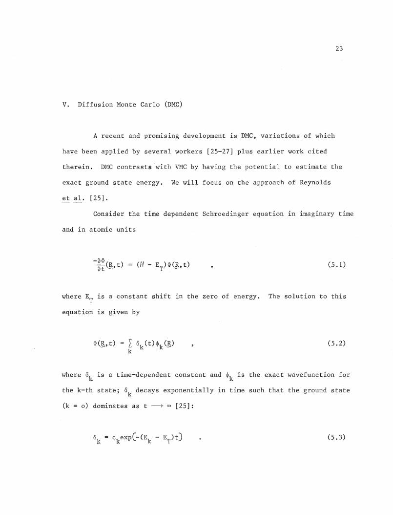
v. Diffusion Monte Carlo (DMC)

A recent and promising development is DMC, variations of which

have been applied by several workers [25-27] plus earlier work cited

therein. DMC contrasts'with VMC by havi~g the potential to estimate the

exact ground state energy. We will focus on the approach of Reynolds

et ale [25].

Consider the time dependent Schroedinger equation in imaginary time

and in atomic units

-d<P-;-(R, t)at -"

(5.1)

where ET

is a constant shift in the zero of energy_ The solution to this

equation is given by

(5.2)

where ok is a time-dependent constant and ~k is the exact wavefunction for

the k-th state; ok decays exponentially in time such that the ground state

(k = 0) dominates as t· w--+ 00 [25]:

(5.3)

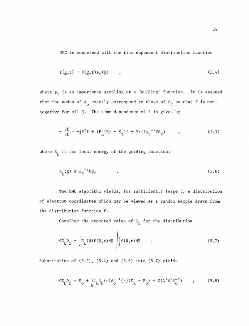
24

DMC is concerned with the time dependent distribution function

(5.4)

where t/lT 1S an importance sampling or a "guiding" function. It is assumed

that the nodes of ~o exactly correspond to those of t/lT so that f is non­

negative for all g. The time dependence of f is given by

(5.5)

where EL

is the local energy of the guiding function:

(5.6)

The DMC algorithm yields, for sufficiently larget, a distribution

of electron coordinates which may be viewed as a random sample drawn from

the distribution function f.

Consider the expected value of EL

for the distribution

(5.7)

Substitution of (5.2), (5.4) and (5.6) into (5.7) yields

(5.8)

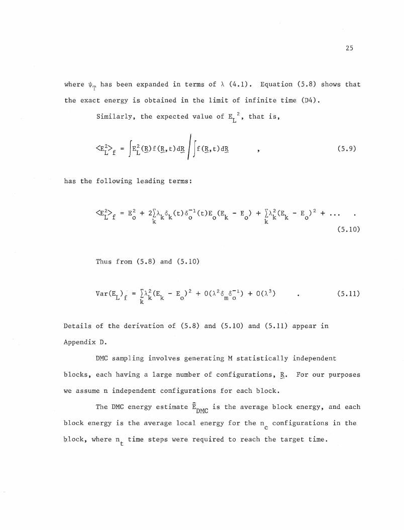
25

where ~T has been expanded in terms of A (4.1). Equation (5.8) shows that

the exact energy is obtained in the limit of infinite time (D4).

Similarly, the expected value of EL2

, that is,

(5.9)

has the following leading terms:

(5.10)

Thus from (5.8) and (5.10)

(5.11)

Details of the derivation of (5.8) and (5.10) and (5.11) appear in

Appendix D.

DMC sampling involves generating M statistically independent

blocks, each having a large number of configurations,~. For our purposes

we assume n independent configurations for each block.

The DMC energy estimate iD~ is the average block energy, and each

block energy 1S the average local energy for the n configurations in thec

~lock, where n time steps were required to reach the target time.t

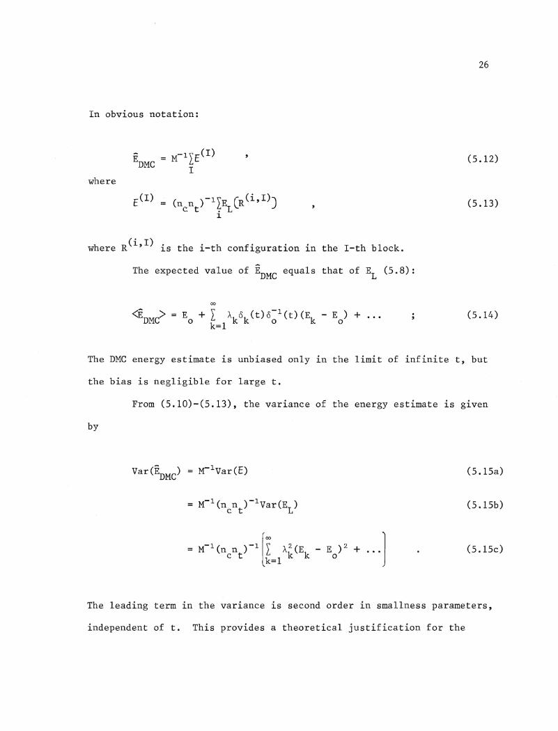
26

In obvious notation:

where

(ncnt)-l?ELCR(i~I))1

h R(i,I). h · h f· .. h h bl kwere 18 t e 1-t con 19urat10n 1n t e I-t oc.

The expected value of EDMC equals that of EL (5.8):

00

(5.12)

(5.13)

+ ... (5.14)

The DMC energy estimate is unbiased only in the limit of infinite t, but

the bias is negligible for large t.

From (5.10)-(5.13), the variance of the energy estimate is given

by

=M-1(nn)-1[I .A 2 (E -E)2+ ••• ]c t k=l k k 0

(S.15a)

(5.1Sb)

(5.15c)

The leading term in the variance 1S second order in smallness parameters,

independent of t. This pro~ides a theoretical justification for the

27

empirical observation of Reynolds et al. [25] that the precision of DMC

calculations is strongly dependent on the choice of WTe

28

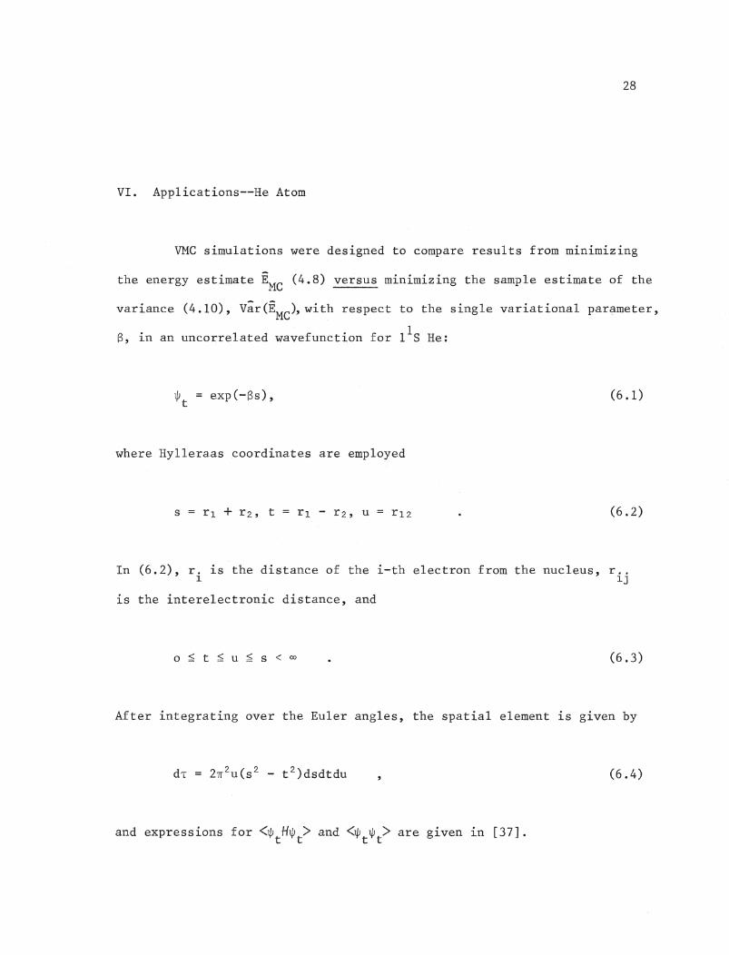
VI. Applications--He Atom

VMC simulations were designed to compare results from minimizing

the energy estimate EMC (4.8) versus minimizing the sample estimate of the

variance (4.10), Var(EMC),with respect to the single variational par.;itmeter,

S, in an uncorrelated wavefunction for lIS He:

1jJt exp(-Ss), (6.1)

where Hylleraas coordinates are employed

(6.2)

In (6.2), r. is the distance of the i-th electron from the nucleus, r ..1 1J

is the interelectronic distance, and

o ~ t ~ u ~ s < 00 (6.3)

After integrating over the Euler angles, the spatial element is given by

(6.4)

and expressions for <1jJ H¢ > and <¢ ¢t> are given in [37].t t t

29

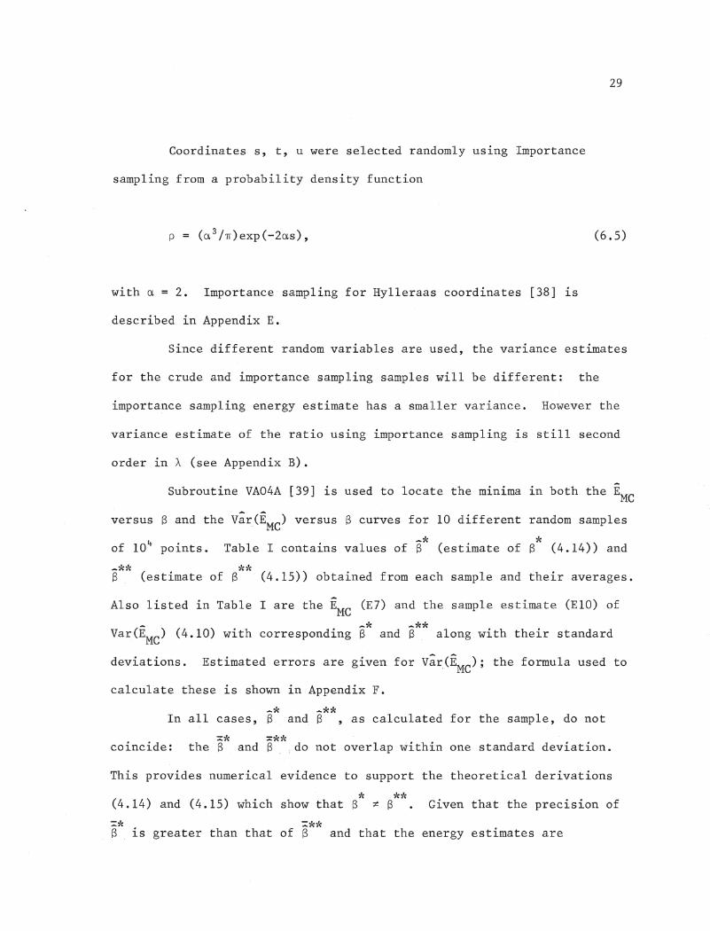
Coordinates s, t, u were selected randomly using Importance

sampling from a probability density function

p (a 3 /1T)exp(-2as), (6.5)

with a = 2. Importance sampling for Hylleraas coordinates [38] is

described in Appendix E.

Since different random variables are used, the variance estimates

for the crude and importance sampling samples will be different: the

importance sampling energy estimate has a smaller variance. However the

variance estimate of the ratio using importance sampling is still second

order in A (see Appendix B).

Subroutine VA04A [39] is used to locate the minima in both the EMC

versus B and the V~r(EMC) versus B curves for 10 different random samples

of 10 4 points. -* *Table I contains values of S (estimate of S (4.14)) and

-** **S (estimate of S (4.15)) obtained from each sample and their averages.

Also listed in Table I are the EMC

(E7) and the sample estimate (E10) of

- -* -**Var(EMC

) (4.10) with corresponding Sand S along with their standard

deviations. Estimated errors are given for V~r(EMC); the formula used to

calculate these is shown in Appendix F.

_* _'1<*In all cases, Sand S ,as calculated for the sample, do not

::*;'< :::'1< '1<coincide: the Band S do not overlap within one standard deviation.

This provides numerical evidence to support the theoretical derivations

'1< 'I<*;,<(4.14) and (4.15) which show that B ~ S Given that the precision of

=* =**S is greater than that of S and that the energy estimates are

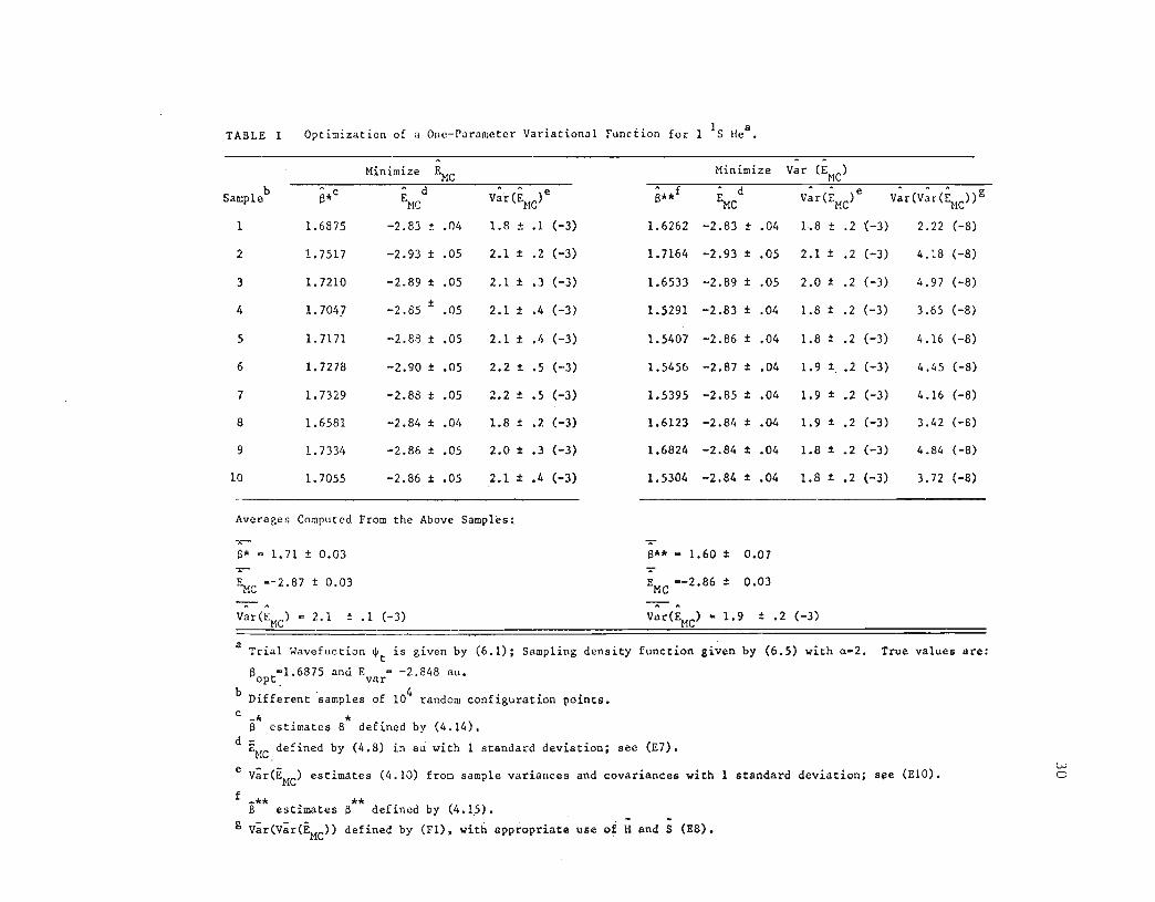
TABLE I ~Y~4~4~~~ion of a Onc-Parameter Variational Function for 1 IS

"'"

V~r(v~r(~c})g

1 ± .1 (-3) 1.6262 -2.83 ± ,.04 1·.8 ± .2 {-3) 2.22 (-8)

1 ± .2 (-3) 1.7164 -2.93 ± 05 2.1 ± .2 (-3) 4 .. 18 (-8)

1 ± .3 (-3) 1.6533 -2.89 ± .05 2 .. 0 ± .2 (-3) 4.97 (-8)

2.1 ± .4 (-3) 1 .. 5291 -2.83 ± .04 1.8 ± .2 (-3) 3.65 (-8)

1 (-J) 1.5407 -2.86 :.t .04 1.8 ± .2 (-3) 4.16 (-8)

2.2 1: .5 1. -2.87 :t .04 1.9 t, .2 (-3) 4 .. 45 (-8)

2.2 ± .S (-3) 1.5395 -2.85 ± .04 1.9 ± .. 2 (-3) 4 .. 16 (-8)

1.8 1.6123 -2.84 ± .04 1.9 :1: .2 (-3) 3.42 (-8)

± .3 (-) 1.6824 -2.84 ± .04 1 .. 8 ± .. 2 (-) 4 .. 84 (-8)

2. (-3) 1.. 5304 -2.84 ± .04 1.8 t .2 (-3) 3.72 (-8).05

.,05

-2.

-2.93 ± .05

-2.90 .05

-2 .. 89 .05

-2.85 ±

-2. ±

-2.86 ± .05

1 ..

the Above t.1a.Ull-l4CO

B** 1.. 60 ± 0.01~

--2.86 ± 0.03

LVo

(-3)

by (6.5) with a-2. True values are:

Hand S (E8).appropriate use

by (6.1); WGWtJ'.r...LU~

.14).

, with 1 deviation; see (E7).

-2.848 a.u.

is

(-3)

defined by

) defined by

estimates (4.10) from variances and covariances with 1 standard deviation; s~e (EIO).

wavetuction

b Diff~rent 'gai~~V~"~Q

e

31

comparable (both EMC values are within one standard deviation of Evar)

there would seem to be no reason to choose the Var(EMC ) as a minimization

criterion.

Further studies using a 3-parameter Hylleraas wavefunction [37]

also led to the same conclusions as those provided by the above example.

While it was possible to use minimization of EMC to optimize the

wavefunction, it was found that the sensitivity of the Var(EMC ) to changes

in the parameters made it expensive and impractical to use this

-*';~optimization scheme. It was apparent in this case also that ~ would not

_1<be the same as ~ for a given sample.

An attempt was also made to optimize the normalized v·ersion of

(6.1) using the Var(EMC ) criterion. This proved to be impossible, as

consistently went to very large values, making $ zero and hencet

Var(EMC ) zero also. As this result is due, in part, to the extreme

simplicity of the wavefunction (6.1), it is difficult to -ex:trapolate to

the case of a more complicated, normalized $tft However, these results

concur with the theoretical result (4.19), which being zero-th order in A,

**would provide a different estimate of S than would (4.13). It is also

of note that (4.19) predicts a larger variance than (4.13) which is in

practice true, since the ratio estimator uses correlation between the

numerator and denominator to reduce its variance.

32

VII. van der Waals Interaction Energy: An Electron Correlation Problem

33

"supermolecule" EAB

(consisting of the interacting subsystems A and B

separated by distance R) and the sum of the non-interacting subsystem

energies EA

and EB

.

(7.1)

'When R is the equilibrium distance Re , ~EINT(Re) is the van der Waals

binding energy. In general, if neutral, non-polar molecules/atoms A and

B are considered, the existence of a minimum in the inter-molecular/atomic

energy versus distance R curve is almost entirely a manifestation of

inter-molecular/atomic correlation energy. (In the Perturbation scheme,

this is called the dispersion energy.) Correlation energy arises

because coulombic repulsion between like charges tends to keep electrons

apart, thus lowering the total energy of a systeme In the simple

Hartree-Fock Self-Consistent-Field (HF-SCF) theory, Fermi correlation (a

consequence of the Pauli Exclusion Principle--two electrons with like spin

cannot exist in the same spatial orbital) is accounted for by requiring

the molecular wavefunction to be antisymmetric. However, correlation

between electrons with unlike spins (Coulumbic correlation) is not

considered and so the term correlation energy refers to the difference

between the true energy and the Hartree-Fock energy EHF -

Typically, correlation energy makes up less than one percent of

the total energy and although for qualitative purposes it can often be

34

ignored, properties of chemical interest require its recovery for

quantitative results. One major problem encountered in the variational

treatment is the Basis Set Superposition Error (BSSE) [47-49] which

results in a ~EINT that is too large. This is a purely mathematical

artifact: EAB is calculated with a qualitatively better basis set than

the ones from which EA and EB

are found, simply because basis set AB is a

union of basis sets A and B. Instead of the costly procedure of

expanding the subsystem basis sets to the point where the effect of

doubling the size at Re does not radically improve EAB

, counterpoise

correction or ghost orbitals [48, 49] may be used. Here, EA

and EB

are

computed with basis set AB; that is, the EA

computation is allowed use

of basis set B, but without B actually being present. Studies have shown

that such techniques do not overcorrect [49].

Configuration Interaction (GI) calculations mix contributions

from excited states of the same symmetry with the ground state in order to

recover the correlation energy. The use of explicitly correlated

wavefunctions introduces interelectronic distances r .. into the calculation1J

so that when r .. is small, the wavefunction ~ is small.1J

To get accurate absolute values of the total energy of a quantum

mechanical system is difficult; the absolute error in, say, the He2

problem is greater than the well-depth ~EINT(Re). The Variational

supermolecule approach hinges on the assumption that the error in the

variationally-obtained energy remains constant as a function of the

internuclear separation so that cancel1ation of errors occurs upon

subtraction of the quantities in (7.1). In the He2 problem, the ground

35

state energy is on the order of -5.8 hartree while the well-depth is

about -3.2-3.8 x 10- 5 hartree, and so the absolute error in the

variationally-obtained energies must remain constant to about 1 ppm in

order to get accurate values of ~EINT.

The He2 problem was the first vdW molecule for which good results

were obtained in the early 1970's using CI or MCSCF calculations.

Schaefer and McLaughlin [50] made the assumption that intra-atomic

correlation remains constant over all separations R. Bertoncini and

Wahl [51] included small changes in the intra-atomic correlation energy;

Liu and McLean [52] also incorporated coupling between inter- and intra-

atomic components. Dacre [53] attempted to remove the Basis Set

Superposition Error in addition to incorporating inter- and intra-atomic

correlation. Burton [54] used CEPA-PNO correlated wavefunctions.

Coldwell and Lowther [7] used a very complicated explicitly

correlated wavefunction in a Variational Quantum Monte Carlo calculation.

Their result for ~EINT at Re5.6 au was -3.55 (±0.15) x 10- 5 hartree

as compared to Burton's -3.339 x 10- 5 hartree at R = 5.63 au and to thee

experimental differential-scattering cross-section measurement result of

-3.35 X 10- 5 hartree at R = 5.6 au of Burgmans, Farrar and Lee [55]. Ine

order to obtain such quantitative results for a VMC calculation, sample

sizes of 377',000 and 782,000 points were used.

In the second part of this work, simple explicitly correlated

wavefunctions are examined in a Variational Monte Carlo calculation in

order to see whether a qualitative estimate of ~EINT for He2 can be made.

Quantitative results are not expected as the wavefunctions employed here

36

have only one variational parameter as compared to the hundreds of

parameters used in Coldwell and Lowther's calculation.

Given a partitioning of the Hamiltonian which eliminates the need

for evaluating gradients of an SCF determinant, and the use of well-known

HF-SCF orbital energies, formulae are derived which allow the method to

be applied to He2. A method of Importance sampling in prolate spheroidal

coordinates is derived and the whole incorporated into a computer program.

Results from the first part-of this work are used to optimize the

correlated wavefunctions.

37

VIII. Theory

(a) Partitioning of the Hamiltonian-Combining Results from HF-SCF and

Correlation Functions

From HF-SCF theory [56], the i-th spin orbital ¢. is an eigenfunction~

of the effective Hamiltonian H:ff :~

E.¢.(l)~ ~

i 1, ••• , N (8.1)

where ¢. ~s a product of a spatial function f. and spin component a or S:~ ~

¢. (x)~

(8.2)

and 1 represents the space and spin coordinates of electron 1, E. is the~

orbital energy. There are N such equations for the N orthonormal spin-

orbitals in the N-electron system.

E. :~

Thus the expectation value of H:ff is~

E.~

i 1, ... , N (8.3)

More explicitly,

<~.(l) IB~ffl~.(l» _ <~.(l) lB. I~.(l» + J. K.,~ ~ ~ ~ ~ ~ ~ ~

~ 1, ... , N (8.4)

where

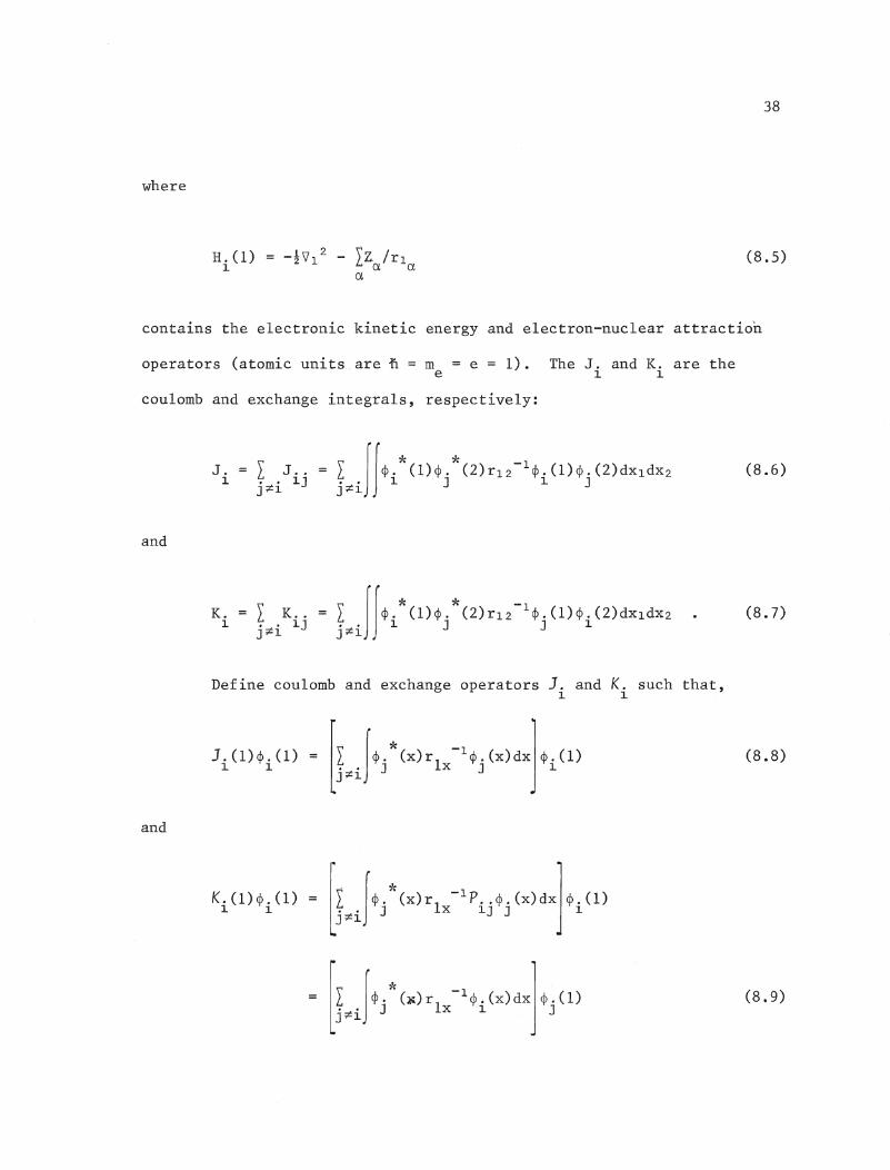
38

H. (1)1

(8.5)

contains the electronic kinetic energy and electron-nuclear attraction

operators (atomic units are n = m = e = 1). The J. and K. are thee 1 1

coulomb and exchange integrals, respectively:

and

t· \ II * * -1J. = L J .. = L ¢. (1)¢. (2)rI2 ¢.(1)¢.(2) dx l dX 21 •• 1J •• 1 J 1 J

J 7:1 J 7:1

(8.6)

K.1

I K ..• · 1JJ7:1

(8.7)

Define coulomb and exchange operators J. and K. such that,1 1

and

J.(l)¢.(l)1 1

K.(l)¢.(l)1 1

. I "l<I ¢. (x)r1

-lp . .¢.(x)dx ¢.(l)• • JX 1J J 1J7:1

(8.8)

(8.9)

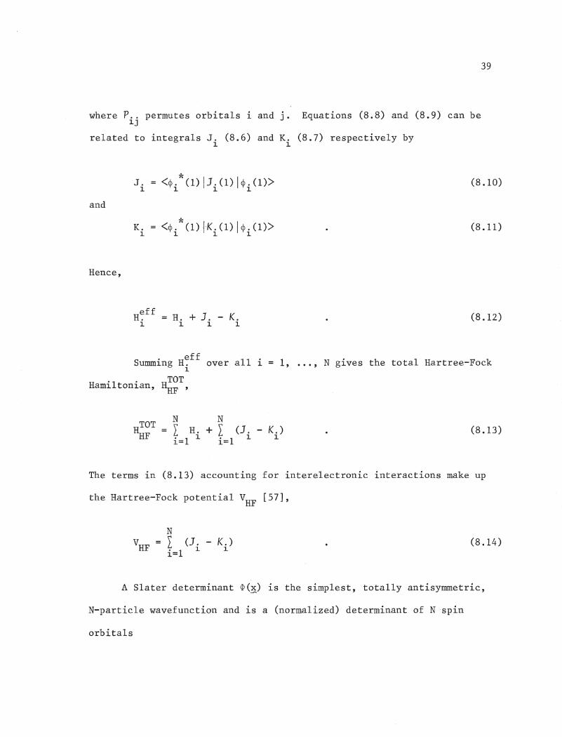
39

where P.. permutes orbitals i and j. Equations (8.8) and (8.9) can be1J

related to integrals J. (8.6) and K. (8.7) respectively by1 1

and

Hence,

J.1

K.1

eJ~

<¢. ( 1) IJ · (1) I¢ . (1)>111.

,;t.

<¢. ~ (1) l-<K. (1) I¢ . (1)>1. 1. 1.

H.+J.-K.1. 1. 1.

(8.10)

(8.11)

(8.12)

· eff 11 ·Summ1.ng H. over a 1.1.

Hamiltonian, ~~T,

1, ... , N gives the total Hartree-Fock

HTOTHF

N NI H. + I (J. - K.)i=l 1. i=l 1. 1.

(8.13)

The terms in (8.13) accounting for interelectronic interactions make up

the Hartree-Fock potential VHF [57],

NL (J. - K.)i=l 1. 1.

(8.14)

A Slater determinant ~(~) is the simplest, totally antisymmetric,

N-particle wavefunction and is a (normalized) determinant of N spin

orbitals

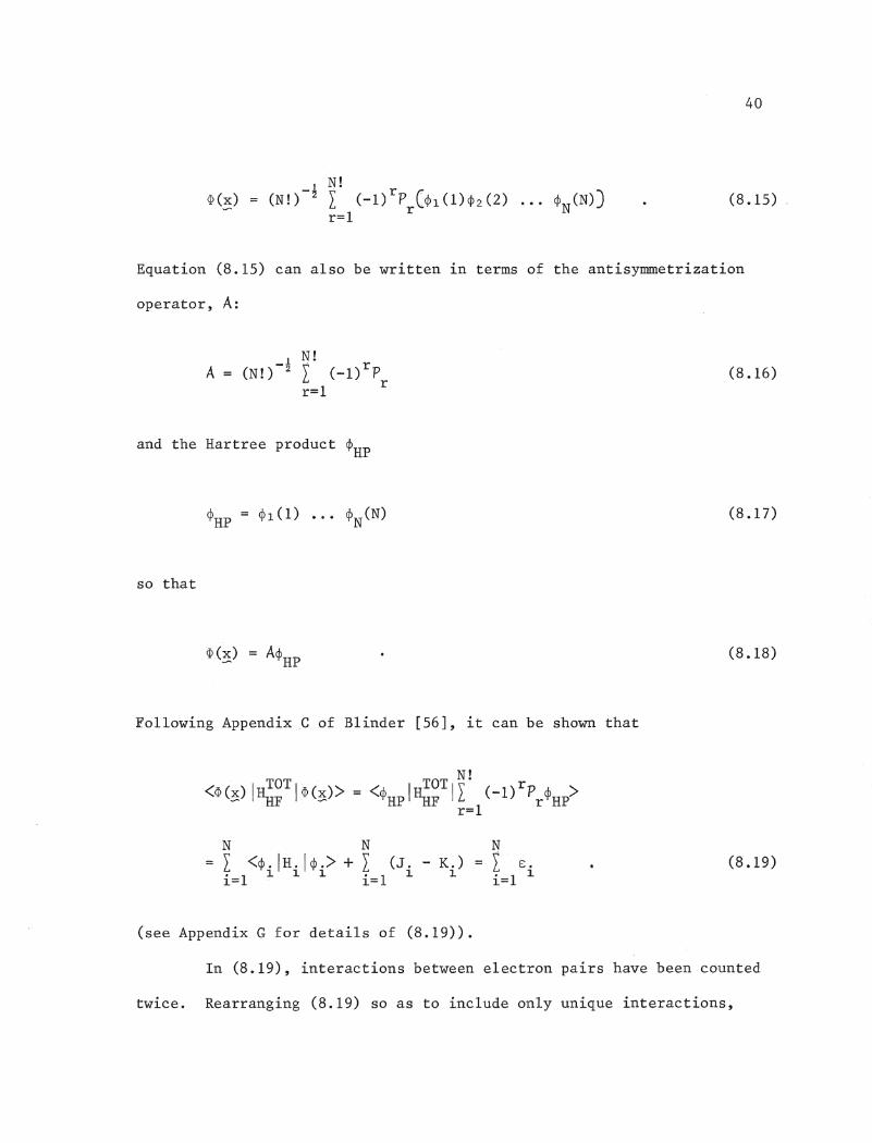
40

(8.15) ,

Equation (8.15) can also be written in terms of the antisymmetrization

operator, A:

_1 N!A = (N!) 2 I (_l)rp

r=l r

and the Hartree product ~HP

so that

Following AppendixC of Blinder [56], it can be shown that

(8.16)

(8.17)

(8.18)

N NI <ep. IH · Iep •> + L (J.... K.)i=l 1 1 1 i=l 1 1

(see Appendix G for details of (8.19)).

NI E.i=l 1

(8.19)

In (8.19), interactions between electron pairs have been counted

twice. Rearranging (8.19) so as to include only unique interactions,

N NI <ep. IH. J <P •> + I I (J .. -- K .. )i=l 1. 1. 1. j>i i=l 1.J 1.J

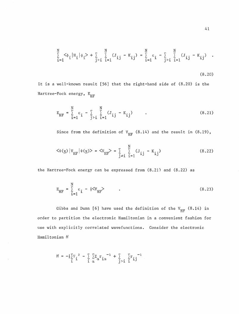
41

N NIE:· - I I (J .. ... K•• )i=l 1. j>i i=l 1.J 1.J

(8.20)

It is a well-known result [56] that the right-hand side of (8.20) is the

Hartree-Fock energy, EHF

N NIE:· - I I (J .. ... K. · )i=l 1. j >i i=l 1.J 1.J

(8.21)

Since from the definition of VHF (8.14) and the result in (8.19),

NL L (J .. -- K.. )j ~i i=l 1.J 1.J

(8.22)

the Hartree-Fock energy can be expressed from (8.21) and (8.22) as

(8.23)

Gibbs and Dunn [6] have used the definition of the VHF (8.14) in

order to partition the electronic Hamiltonian in a convenient fashion for

use with explicitly correlated wavefunctions. Consider the electronic

Hamiltonian H

42

where the first term represents the kinetic operator, the second the

electron-nuclear attraction and the third, the electron-electron repulsion.

Indices i and j refer to summations over electrons; index a refers to

summation over the nuclei. The Hamiltonian can be partitioned as follows:

H[H - I Ir .. -1 + VHF] + [I Ir ..-1

- VHF]j>i i 1J j>i i 1J

(8.24)

(from (8.13) and (8.14)) since addition and subtraction of terms leaves H

unchanged.

Employing ~(~) to evaluate <H> will give the Hartree-Fock energy

for the system. Knowing this, and using (8.24)

NI. s. + <HI>i=l 1.

(8.25)

Comparison of (8.25) and (8.23) shows that

and so for Hartree-Fock wavefunctions,

(8.26)

<I Lr .. -1>j >i i 1J

(8.27)

43

as mentioned by Gibbs and Dunn [6].

Consider now an explicitly correlated wavefunction of the form

U(r .. )<I>(x)LJ --

(8.28)

where as before ~(~) is a Hartree-Fock wavefunction and U(~ij) is a

correlation function in terms of the interelectronic distances r ..• The---1.J

functional form of U(r .. ) will be chosen to be--1.J

UCr .. )---1.J

exp{-u} exp{'.-I Iu{r .. )}.>.. 1JJ 1. 1.(8.29)

The variational energy using ~(~) (8.28) and the partitioned form

of the Hamiltonian (8.24) is

Evar

(8.30)

The numerator of the first term in (8.30) is

Substituting (8.29) for U in (8.31) leads to

(8.31)

44

(8.32)

It is shown in Appendix H that by applying the Divergence Theorem, the

-+- -+-V.ueV.~ terms which arise from (8.32) disappear, leaving

1 1

<HTOT>HF (8.33)

substituting (8.33) into (8.30), the final result is

Evar. 1<·:-+ -+- *Is. + <HI>/<W W> + !I<v.uev.u>/<W W>. 1 .111 1

(8.34)

as in Gibbs and Dunn [6].

The advantages of (8.34) are clear: the HF-SCF orbital energies

are well-known; <HI> involves only multiplicative terms; the gradient of

-+-the determinant ~(~) need not be computed; V.u are easily evaluated.

1

45

(b) Evaluation of <HI>

The calculation of <HI> in (8.34) involves finding the expectation

value over a distribution function determined by the correlated wavefunction

~(~) (8.28). Following the approach in Appendix G, employing the properties

of the antisymmetrizer, the Hermitian property of quantum mechanical

operators and the symmetry of

in the coordinates, the unnormalized <HI> is written

N!<~HpU2(~ .. ) II Ir .. -1 - I(J· - K.) II (_l)rp ~HP>

1J ••• 1J · 1 1 1 rJ>1 1 1 r=

<I Ir .. -1- ~F>

j >i i 1J

(8.35)

The presence of U(r .. ), while explicitly intr@ducing interelectronic"-1J

coordinates which effectively account for Coulombic correlation missing

from the HF-SCF scheme, complicates the evaluation of molecular integrals.

It is no longer possible to separate multiple integrals; it is also true

that while spin-orthogonality allows for the elimination of many integrals,

those that contain spatially orthogonal orbitals also contain a factor of

u2 and so are non-zero. While expressions such as (8.35) may not be

tractable analytically, Monte Carlo Methods can quite easily be used to

numerically compute many-dimensional, inseparable integrals.

46

It is always desirable from the point of efficiency to identify

zero integrals and to eliminate them prior to computation. Many of the

permutations of ~HP in (8.35) cause zero integrals due to spin-orthogonality.

The expansions from the Slater determinant rapidly increase in size with N,

many terms lead to superfluous integrals. It is possible to employ a

product of determinants containing orbitals of like spins [25,26] to

bypass the construction of such terms.

Instead of (8.28) use

where d represents a determinant of orbitals with spin ss

(8.36)

k, e ~ N/2 (8.37)

For example, consider the two-electron problem: the Slater

determinant gives

(8.38)

All integrals involving ~2(1)~1(2) disappear due to spin orthogonality,

that is,

o (8.39)

47

The use of (8.36) uses only

(8.40)

For a four-electron, closed-shell system the Hartree product is

and (8.36) gives

(8.41)

U(r .. )---1J

CPl(1)CPl(3)

CP3(1)CP3(3)x

CP2(2)CP2(4)

CP4(2)CP4(4)

The expansion of (8.42) leads to four terms involving cp.:1

(8.42)

which arise from permutations between orbitals with like spin. The full

4 x 4 Slater determinant produces 4! = 24 terms; the 20 additional terms

to those in (8.43) contain permutations among orbitals with unlike spin.

After operation of an operator which does not affect spin, mUltiplication

by CPHP' these terms will result in zero integrals.

Then from (8.35) and (8.43), for the four-electron system,

48

IX.

(a)

49

1 +Monte Carlo Evaluation of E for E He2var g

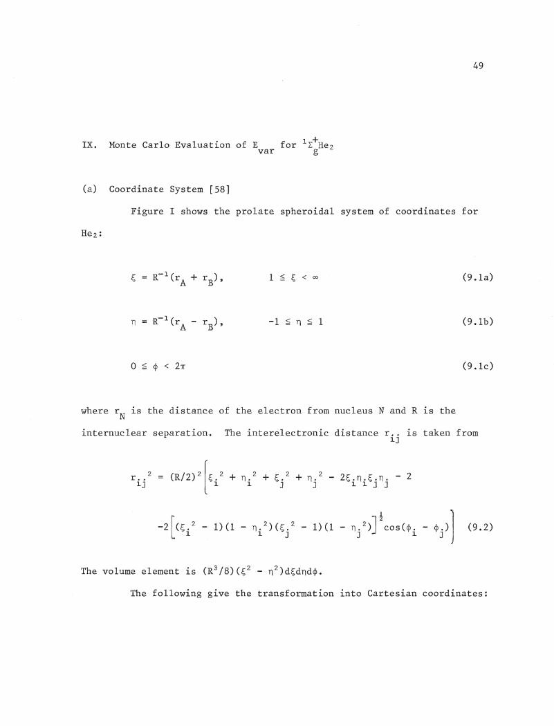
Coordinate System [58]

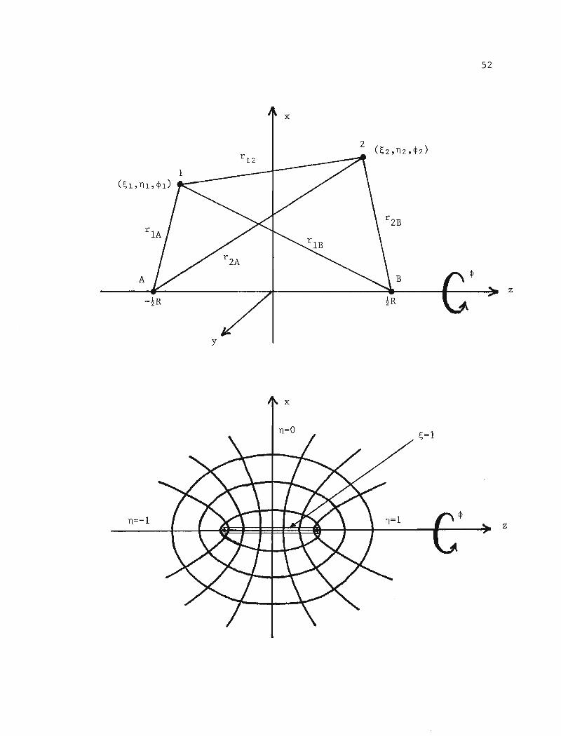
Figure I shows the prolate spheroidal system of coordinates for

n

1 ~ t; < 00

-1 ~ n ~ 1

(9.1a)

(9.1b)

o ~ ¢ < 27T (9.1c)

where rN

is the distance of the electron from nucleus Nand R is the

internuclear separation. The interelectronic distance r .. is taken from~J

The following give the transformation into Cartesian coordinates:

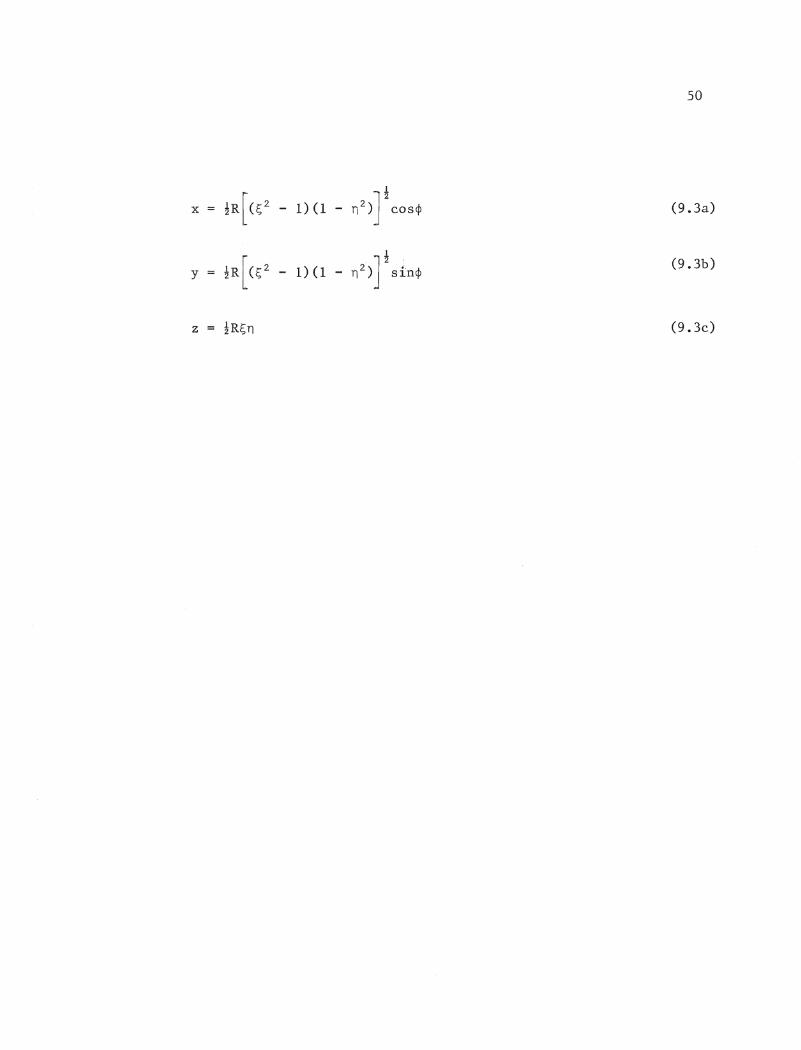
I

X = ~R[(S2 - 1)(1 - n2)J2coS¢

I

Y ~R[(S2 - 1)(1 - n2)J\iri¢

z = !RE;n

50

(9.3a)

(9.3b)

(9.3c)

Figure I. Prolate Spheroidal Coordinate System

51

52

z

z

53

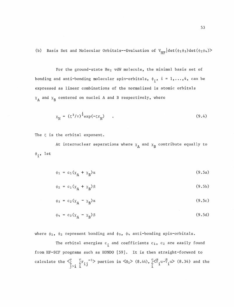
(b) Basis Set and Molecular Orbitals--Evaluation of VHFldet(~1~3)det(~2~4»

For the ground-state He2 vdW molecule, the minimal basis set of

bonding and anti-bonding molecular spin-orbitals, cP., i = 1, .•. ,4, can be1

expressed as linear combinations of the normalized Is atomic orbitals

XA and XB centered on nuclei A and B respectively, where

1

(z;;3/Tf)~exp(-z;;rN)

The ~ is the orbital exponent.

(9.4)

At internuclear separations where XA and XB contribute equally to

cP., let1

cPI CI(XA + xB)a (9.5a)

cP2 CI(XA + XB)S (9.5b)

cP3 C2(XA - X )a (9.5c)B

cP4 C2(XA - XB)S (9.5d)

where cPI' ¢2 represent bonding and cP3' cP4 anti-bonding spin-orbitals.

The orbital energies E. and coefficients CI, C2 are easily found1

from HF-SCF programs such as HONDO [59]. It is then straight-forward to

calculate the <I Ir .. -1> portion in <HI> (8.44), r<~.u.~.u> (8.34) and the. >. . 1J . 1 1J 1 1 1

54

"It:normalization factor <w w> within the Monte Carlo algorithm (IXc) given a

method of sampling in configuration space and formulae for the operators,

U(r .. ) and ¢ .• However, evaluation of---1J 1

4<2: (J. - K.»

i=l 1 1

involves expressing J., K. 1n terms of known analytic functions arising from1 1

atomic orbitals XA and XB•

Consider J 1 ; from (8.8)

f~~(X)rlX-l~2(X)dX+ f~~(X)rlX-l~3(X)dX

+ f~~(X)rlX-l~4(X)dX (9.6)

Substitution of (9.5b-d) into (9~e) and allowing that XA

and XB are real,

gives

(9.7)

where the spin-components have been integrated over, and terms collected.

A like expression is found for J 2 (1) and

(9.8)

55

(2C 12 + C2

2) [XA2(rX)rlX-ldrX + [XB2(rx)rlx-ldrx]

+ 2(2c 12 - C22)[XA(rX)XB(rX)rlX-ldrX

Roothan [60] gives a formula for

[Xl 2(r )r

1-ldr

s x x x

the integration over coordinate r amounts to finding the potential forx

electron 1 at its instantaneous position in space due to the charge

distribution X1s2. This potential is, for a (ls)2 charge distribution,

(9.9)

where rl is the electron-nuclear separation.

Rlidenberg [61] gives general formulae for two-center exchange

integrals for Slater-type atomic orbitals which can be modified somewhat to

calculate

It 1.S shown in Appendix I that, for XAXB

56

r

JXACrX)XBCrX)r1X-ldrX

~ ( )! 2 ~2R- 1 CRs)3I C2t + 1)/2J ptCnl)I I w .B.OtCO)

~=o n=O j=O nJ J

x [QtC~l)KtnC~l'SR) + PtC~l)LtnC~l'SR)] (9.10)

where P2 and Q2 are the Legendre polynomials of the first and second kind,

respectively; K2n

and L2n

are given by:

~1

KtnC~l,a) = J expC-a~)~nptC~)d~1

and

JOO expC-al)~nQtC~)d~~1

Coefficients w • are given in Table I of Rudenberg [61] and B.OtCO)nJ J

defined as

1

[C2t + 1)/2)!J ptCn)njdn

-1

In a similar manner, Kl~. is from (8.9)1

(9.11)

(9.12)

are

(9.13)

(9.14)

J~:CX)r1X-l~lCX)dX~2(1) + J~:CX)r1X-l~1(X)dX .3(1)

+ [J~~CX)r1X-l~lCX)dX]~4C1)

57

Now, the first and third integrals in (9.14) are zero due to spin-

orthogonality; only the term which permutes orbitals with like spin remains.

Substituting (9.5i)~ (9.5d) into (9.14) and integrating over spin leaves

(9.15)

Similarly,

(9.16)

(9.17)

(9.18)

Expressions (9.7), (9.8), (9.15)-(9.18) are used in (8.44); terms

arising from the expansion of

(9.19)

are shown in Appendix J.

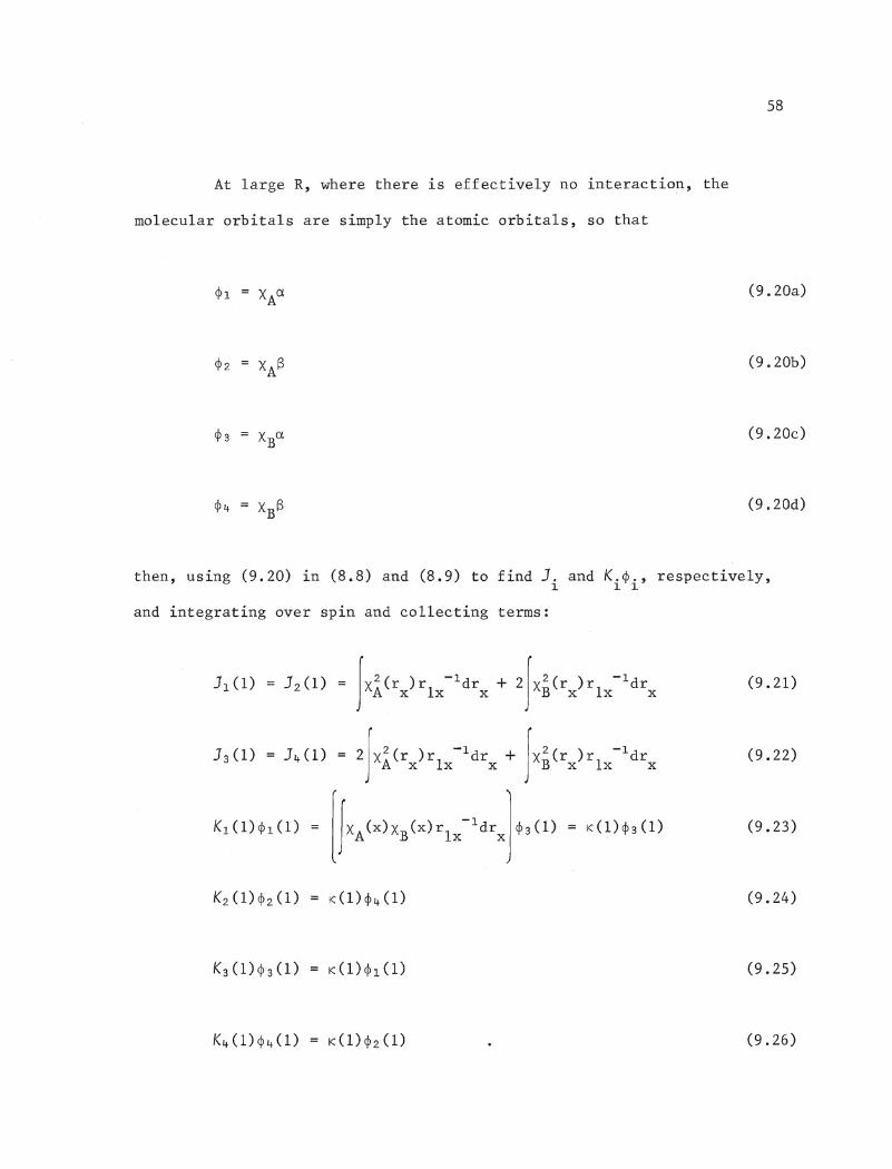
58

At large R, where there is effectively no interaction, the

molecular orbitals are simply the atomic orbitals, so that

(9.20a)

(9.20b)

(9.20c)

(9.20d)

then, using (9.20) in (8.8) and (8.9) to find J. and K.¢., respectively,1 11

and integrating over spin and collecting terms:

JxiCrX)rlX-ldrx + 2JX~CrX)rlX-ldrx

J4 (1) = 2Jx 2 (r)r -ldr + Jx 2 (r)r -ldrA x Ix x B x Ix x

(9.21)

(9.22)

(9.23)

(9.24)

(9.25)

(9.26)

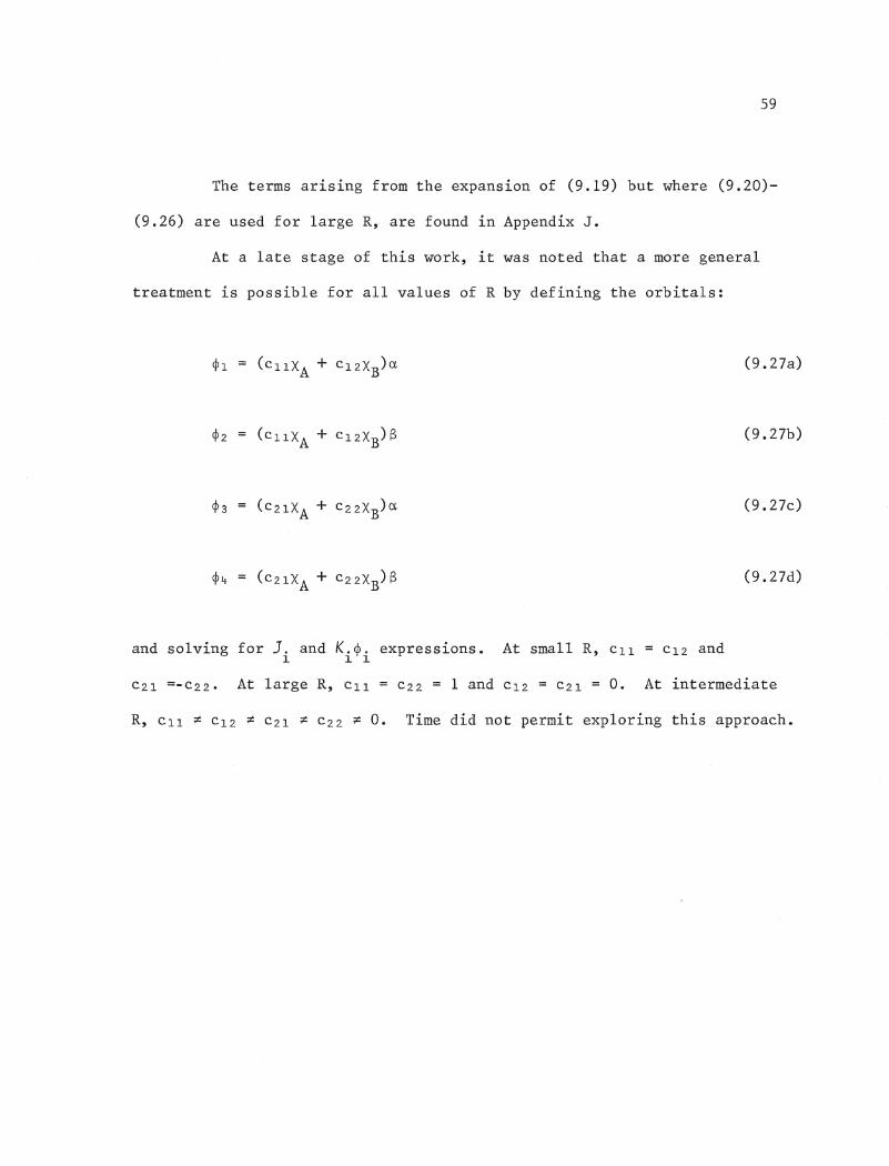
59

The terms arising from the expansion of (9.19) but where (9.20)-

(9.26) are used for large R, are found in Appendix J.

At a late stage of this work, it was noted that a more general

treatment is possible for all values of R by defining the orbitals:

CP3

(9.27a)

(9.27b)

(9.27c)

(9.27d)

and solving for J. and K.¢. expressions. At small R, CII = Cl2 and~ 1 1

C2I =-C22. At large R, ell C22 = 1 and C12 = C2I = O. At intermediate

R, ell ~ cl2 ~ C21 ~ C22 ~ o. Time did not permit exploring this approach.

60

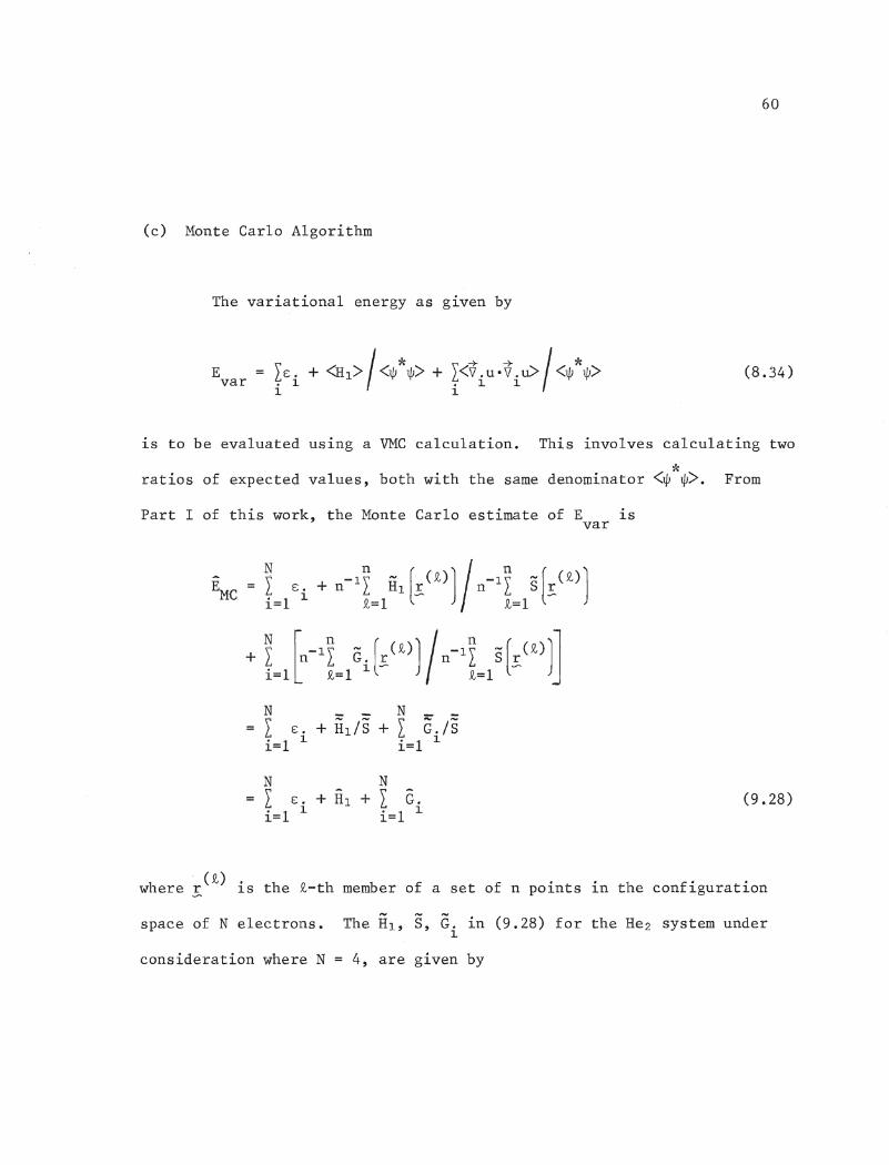
(c) Monte Carlo Algorithm

The variational energy as given by

Evar (8.34)

1S to be evaluated using a VMC calculation. This involves calculating two

ratios of expected values, both with the same denominator <~*~>. From

Part I of this work, the Monte Carlo estimate of E isvar

N NI €. + HIls + I G./si=l 1 i=l 1

N NI €. + HI. + L G.i=l 1 i=l 1

(9.28)

. (2)where ~ is the 2-th member of a set of n points in the configuration

space of N electrons.,.., ,.., ,..,

The HI, S, G. in (9.28) for the He2 system under1

consideration where N = 4, are given by

,.."

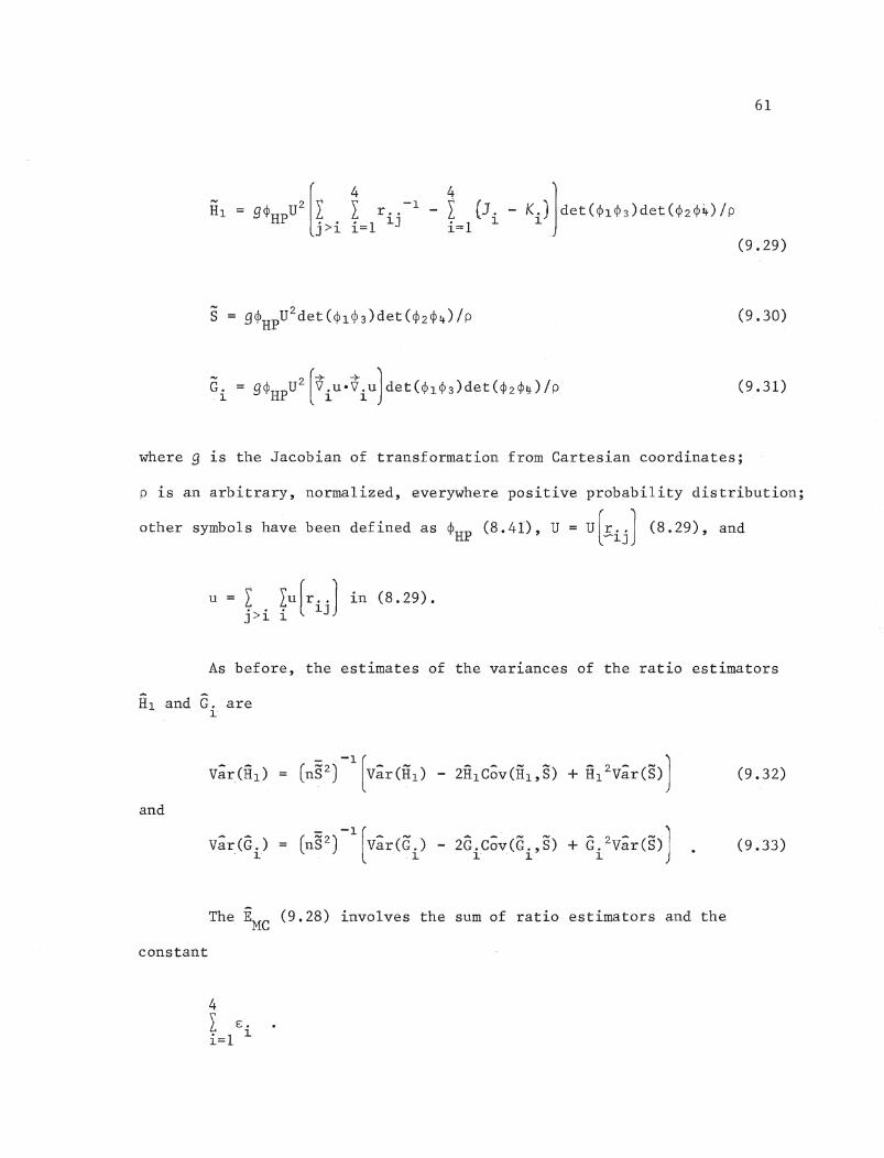
S

g~HPU2[~ ! r .. -1

- 1 (J.j>i i=l ~J i=l ~

61

Ki)]det(~1~3)det(~2~~)JP(9.29)

(9.30)

(9.31)

where 9 is the Jacobian of transformation from Cartesian coordinates;

p is an arbitrary, normalized, everywhere positive probability distribution;

other symbols have been defined as ~HP (8.41), U = U[~ijJ (8.29), and

u = ~ Lu[r .. J in (8.29).j >i i ~J

As before, the estimates of the variances of the ratio estimators

HI. and G. are~

(9.32)

and

(9.33)

The EMC

(9.28) involves the sum of ratio estimators and the

constant

4I s.i=l ~

62

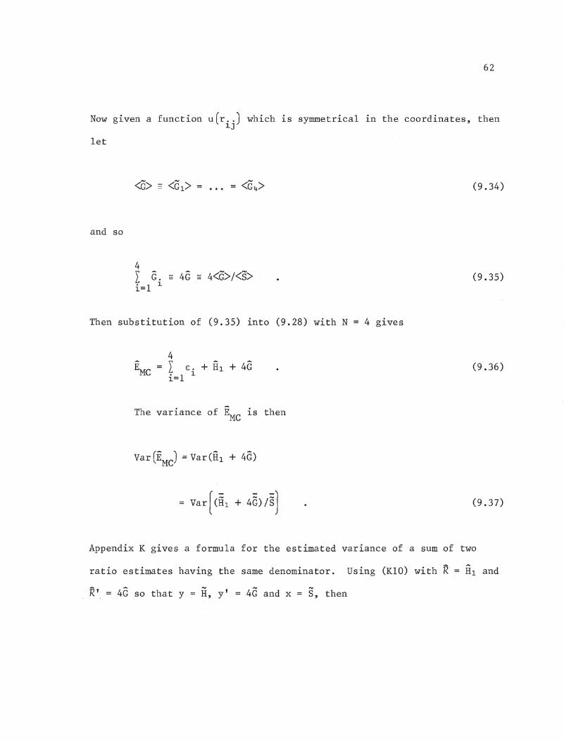
Now given a function u(r .. ) which is symmetrical in the coordinates, then1J

let

. " .. (9.34)

and so

4I G. - 4G - 4<G>I<5>i=1 l'

Then substitution of (9.35) into (9.28) with N

4EMC I E: • + HI + 4G

i=l 1

The variance of EMC is then

4 gives

(9.35)

(9.36)

(9.37)

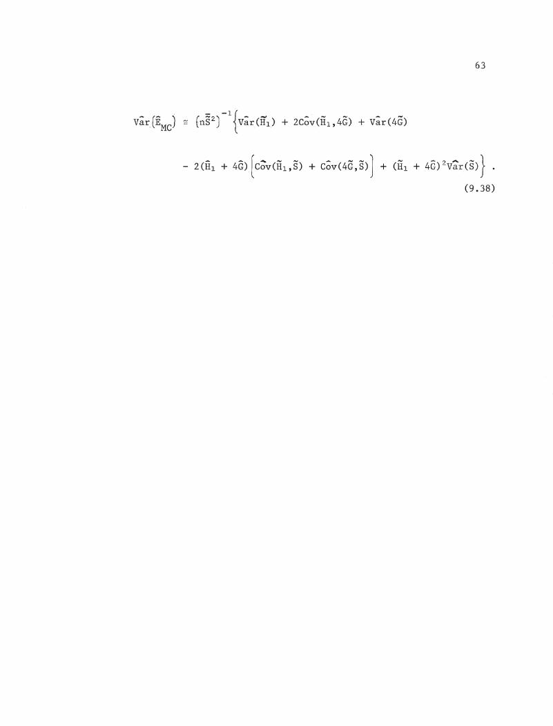
Appendix K gives a formula for the estimated variance of a sum of two

ratio estimates having the same denominator. Using (KIO) with R = HI and

R' = 4G so that y = H, y' = 4G and x = S, then

63

- 2(ih + 4G)(C;;'V(HI,S) + COV(4C,S)) + (HI + 4G)2V;;:r(S)} .

(9.38)

64

x. Monte Carlo estimate of ~EINT--Correlated Sampling

Consider the VMC calculation of the interaction energy, ~EINT;

the ~nte Carlo estimate of AE1NT (7.1), AiMC is given by

(10.1)

where R is sufficiently large internuclear separation so that the two00

subsystems are not interacting; ET is the total energy

where ENN

is the nuclear-nuclear repulsion term equivalent to

(in this case ENN 4R- 1 ). h · h l·- TeET ~s t e Monte Car 0 est1mate of ET,

(10.3)

where EMC

is given by (9.36). Because ENN

is a constant,

(10.4)

65

If two independent runs are made to find ET(R) and ET(R,), then

the variance of ~EMC(R) is the sum of the variances of the two estimates:

(10.5)

This is likely to be significant, especially since ~EMC(R) is much less

than either ET(R) or ET(R). A powerful method of variance reduction is

Correlated sampling [62] in which the same set of random numbers are used

to calculate both EMC(R) and EMC(Roo). The objective is to create a high

positive correlation between the samples which causes

(10.6)

to be much less than var(~EMC(R)) given by (l0.5), where independent

samples cause the covariance term in (10.6) to be zero.

In this situation, the easiest method of creating positive

( .)correlation is to use the same set of random numbers R. 1. to generate

configuration points E(R) (0 and E(RJ (i) used to calculate EMC(R) and

EMC(Roo)' respectively. If the Importance sampling functions used to

, (R) (i) d (R)' (i) ··1 h h 1 fgenerate E. an E. 00 are 8l.mJ. ar, t en t e two samp es 0

configuration points will be correlated and so will EMC(R) and EMC (RJ •

The one complication added by the use of Correlated sampling is

in calculating the cov(EMC(R),EMC(Roo)} term in (10.6). While in principle

66

this is easily found, in practice it entails that either (i) simultaneous

simulations be run so that a cumulative calculation of the covariance can

be made, or (ii) separate simulations be run but storage of ~~)(R) and

E~~) (Roo)' i = 1, ••• , n, allows a later computation of the covariance. In

the former case, a restriction on computer time may be a problem and in

the latter, large amounts of storage space are necessary.

From (9.36) and (10.1),

4I (E. (R)i=l 1

(10.7)

which involves differences between ratio estimates with different

denominators. Appendix K provides a formula (K12) which can be used to

estimate Var(R - R') where

- (~I (R) 4a(R)) I§(R)R + (10.8)

and

R' (HI (RJ + 4G (RJ) Is (RJ (10.9)

and (KID) is used to find both V~r(R) and V~r(R'). Equation (K13) is

used to find c~v(R"R') where y = HI (R) + 4G(R), x = S(R),

67

XI. Choice of Correlated Function--Simulations of SCF Results

--Optimization of ~(x)-VMC Results

(a) Choice of U(r .. )---lJ

The wavefunction chosen for the VMC calculations is described by

(8.43) where the spin orbitals ~. for small and large internuclear1

separations are given by (9.5) and (9.20), respectively; atomic orbitals

XA and XB are given by (9.4) with s = 1.69, the optimized orbital

exponent for an STO describing He.

For these initial studies, two simple correlation functions,

U(r .. ) (8.29) were chosen on the basis of other calculations found in the"""'lJ

literature. These are

and

1(1 + br .. )J1J(11.1)

expl(-~ . Iuer .. )]·J >1 i 1J

c 2 r .. ]'1J

(11.2)

where a, b, c are variational parameters. Equation (11.1) is an example

of a Jastrow function [63]; Moskowitz and Kalos [26], Handy [64],

Reynolds et ale [25] have employed functions of th~s type in atomic

and molecular (chemically bound systems) calculations. This Pade form

68

obeys the electron-electron cusp condition, which requires u(r .. ) to be1.J

linear in r .. at small r .. , and the requirement that u(r .. ) asymptotically1.J 1.J 1.J

approach a constant and be of the order O(r .. - 1 ) so that the wavefunction1.J

factors at large r .. [25, 65].1.J

The second U(r .. ) (11.2) has been used by Gibbs and Dunn [6] in a'""1.J

calculation of C2+. It also has the aforementioned properties as (11.1)

at small and large r ... * Other functional forms for the correlation1.J

function [66] have not been examined by this work.

-+ -+Appendix L contains expressions for V.u-V.u for both (11.1) and

1. 1.

(11.2) •

* After calculations using (11.2) had been made, it was noted that

(11.2) is not unitless. Further investigation into references quoted by

Gibbs and Dunn [67, 68] lead to speculation that a misprint was made in

[6] and that the functional form of (11.2) would more properly involve

something such as

I Ia(l - exp(-cree))r .. - 1

j>i i 1.J 1.J

The use of an incorrect correlation function would, of course, invalidate

the results found in (XIc) and in Tables III and IV.

69

(b) Computer Program--Simulation of SCF Results for He2

The HF-SCF program HONDO [59] was run on the Burroughs 6700 in

order to obtain orbital energies, s., molecular coefficien~Cl and C2~

(9.5) and the SCF results for He2 at various internuclear separations

between 1 au and 14 au. The calculations employ an STO-6G minimal basis

set (a computational check was performed to ensure that the particular

combination of Gaussians used by HONDO mimic an STO with ~ = 1.69).

The range over which XA and XB

contribute equally to ~i (9.5) lies

below about 9 au. The value of R was taken at 14 au, beyond which the00

atoms were effectively non-interacting «9.20) could be employed).

Points in configuration space used to calculate HI (9.28) and

G (9.36) are chosen using Importance sampling in prolate spheroidal

coordinates. The probability inversion technique is employed; the method

is described in Appendix M.

Computer programs were written in FORTRAN IV to run on the VAX-II/780

in double precision which calculate EMC (9.36), Var{EMC ) (9.38) and other

quantities of interest at small and large R. The Gin (9.36) is computed

as Gl; no attempt was made to compare the G., ~ = 1, •.. ,4, values!)~

Intermediate ranges (9 au < R < 14 au) where (9.20) hold were not

considered. The sample means, variances and covariances are found

cumulatively using an efficients moments routine [69]. Standard

deviations are taken as the square roots of the estimated variances.

70

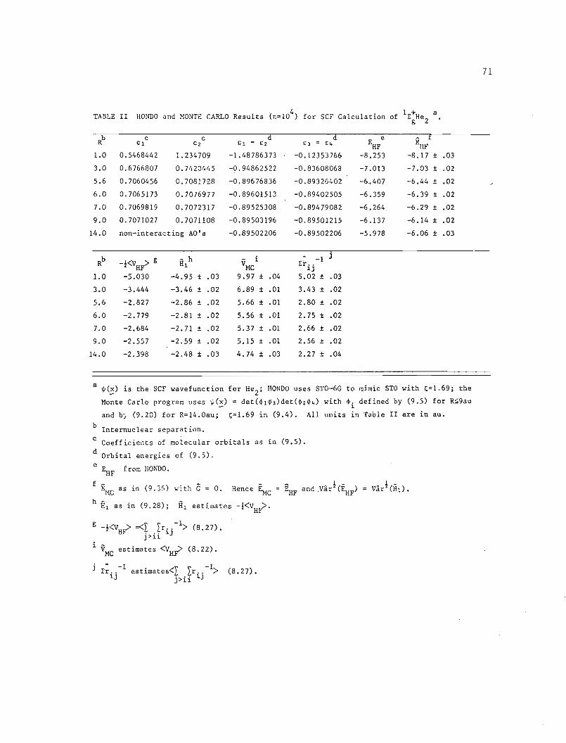
The programs were first used to find the Monte Carlo estimate of

EHF , EHF , that is, where U(!ij) is set to unity so that ~(~) = ~(~) and

4IE. + HIi=I ~

(11.3)

Table II contains values of

- - ..... 1from HONDO and the Monte Carlo ratio estimates, EHF , HI, VMC and Erij

of EHF

,

respectively, given an independent sample of 10 4 points. Also noted are

standard deviations of the ratio estimates (analogous equations to (9.32)

and (9.33) are used to estimate val(vMC ) and varr(Erij - I)).

The advantage of using the combined estimate HI over a separate

- . - -1calculation of ~MC and £r.. is that it is immediately apparent that~J

positive correlation between elements used to calculate VMC

and £'r ....... 1

1J

has reduced the variance of HI. That is, the variance of HI is not

- - ..... 1 -simply the sum of the varianees of VM,C' and £r.,. ' $ Al though HI was, 1.J'

treated as one ratio estimator, appropriate use of (KID) could have been

used to find Var(HI) if the difference of the two ratio estimates VMC

71

TABLE II HONDO and MONTE CARLO Results (n=104) for SCF Calculation of l>:+H ag e Z •

Rb c C d d EHFe E

HFf

Cl C2- £1 = £2 £3 = £4

1.0 0.5468442 1.234709 -1.48786373 -0.12353766 -8.253 -8.17 ± .03

3.0 0.6766807 0.7420445 -0.94862522 -0.83608068 -7.013 -7.03 ± ,,02

5.6 0.7060456 0.7081728 -0.89676836 -0.89326402 -6.. 407 -6.44 ± .02

6.0 0.7065173 0.7076977 -0.89601513 -0.89402505 -6.359 -6.39 ± .02

7.0 0.7069819 0.7072317 -0.89525308 -0.89479082 -6.264 -6.29 ± .02

9.0 0.7071027 0.7071108 -0.89503196 -0 .. 89501215 -6.137 -6.14 ± .02

14.0 non-interacting AC's -0.89502206 -0 .. 89502206 -5 .. 978 -6 .. 06 ± .03

Rb -!<V > g.. h i ....

-1HI VMC Er ...HF l.J

1.0 -5.030 -4 .. 95 ± .03 9.97 ± .04 5.02 ± .03

3.0 -3.444 -3.46 ± .02 6.89 ± .01 3.43 ± .. 02

5 .. 6 -2 .. 827 -2.86 ± .02 5.66 ± .01 2 .. 80 ± •.02

6.0 -2.779 -2.81 ± .02 5 .. 56 ± .01 2.75 ± .02

7.0 -2.684 -2 .. 71 ± .02 5.37 ± .01 2.66 ± .02

9.0 -2.557 -2,,59 ± .02 5.15 ± .. 01 2.56 ± .. 02

14.0 -2 .. 398 -2.48 ± .03 4 .. 74 ± .. 03 2 .. 27 ± .. 04

a ~(~) is the SCF wavefunction for He2

; HONDO uses STO-6G to mimic STO with ~=1.69; the

Monte Carlo program uses = det (~2$4) with defined by (9.5) for RS9au

and b~ (9.20) for R=14.0au; t=1.69 in (9.4). All units in Table II are in au ..

b Internuclear Sel)aI'at10Il.

andHence

estimates

as in (9 36) with G

as in (9.28);

C Coefficients of molecular orbitals as in (9.5).

d Orbital energies of (9.5)

e EHF

from HONDO.

f

h

(8.27).

i --.V

MCestimates (8.

- -1l:r ..

1J(8.27) ..

72

and Er .. - I had been employed., 1J

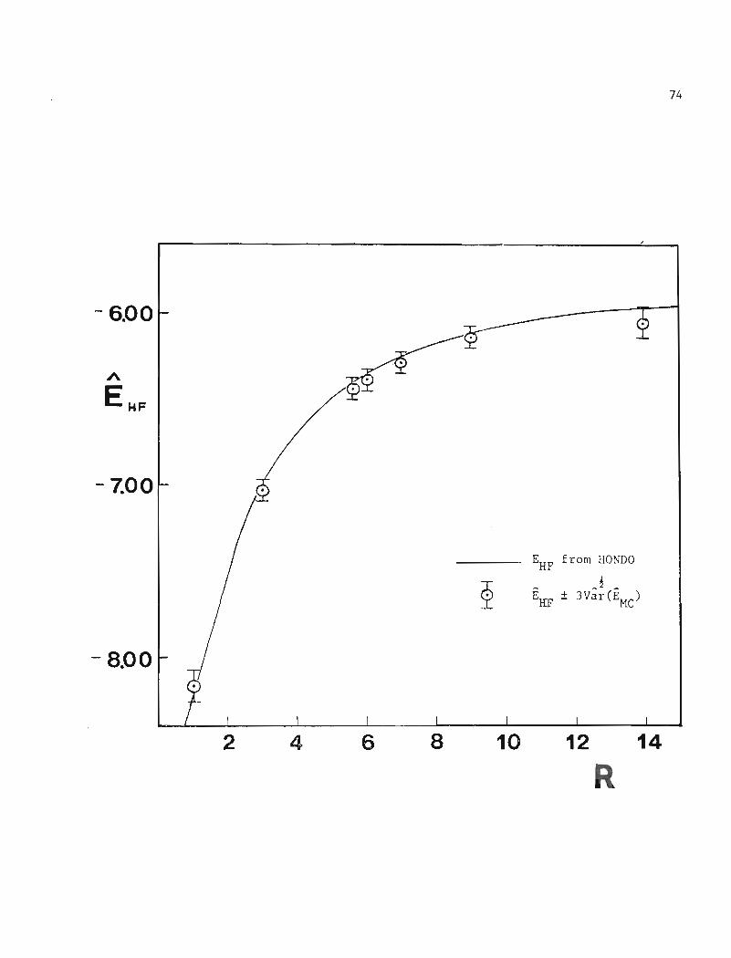
All the SCF results lie within three standard deviations of the

Monte Carlo estimates; the three standard deviation confidence intervals

of HI and _~~ .. -l overlap. Figure II is a plot of the Hartree-Fock1J

energy, EHF

and the Monte Carlo estimate EHF

versus R, along with_ 1 ~

3Var 2 (EHF

) confidence intervals.

Figure II. Monte Carlo Estimate EHF of the

Hartree-Fock Energy versus Internuclear

Separation R for HeZ

73

A

F

±

74

)

75

(c) Optimization of W(~)--Calculationof ~EMC

The accepted minimum in the energy versus internuclear separation

curve falls at about 5.6 au [50~55] which is where Coldwell and Lowther

[7] decided to optimize their wavefunction. Using the results from Part

I of this work, the variational parameters in U(r .. ) of the explicitly'"""'1.J

correlated wavefunction were to be optimized by finding the minimum

Parameter a in the first correlation function was set to 0.5*

(W(~) then rigorously obeys the cusp condition) and optimization with

respect to b was attempted using a sample of 10 3 configuration points and

subroutine VA04A [39]. This was not successful as no minimum was found:

b was sent to increasingly large values. This raised the question as to

the suitability of (11.1) for this calculation, which is addressed in

the discussion section, Chapter XII.

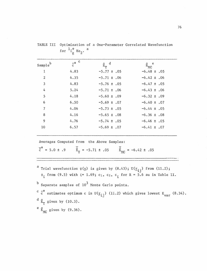
It was possible to optimize the wavefunction with respect to

parameter c of (11.2). -*Table III contains values of c (estimate of

optimal value of c) and corresponding values of EMC {with one standard

deviation) and ET for 10 different samples of 10 3• =*The average c and

- -EMC and Er with standard deviations are also shown.

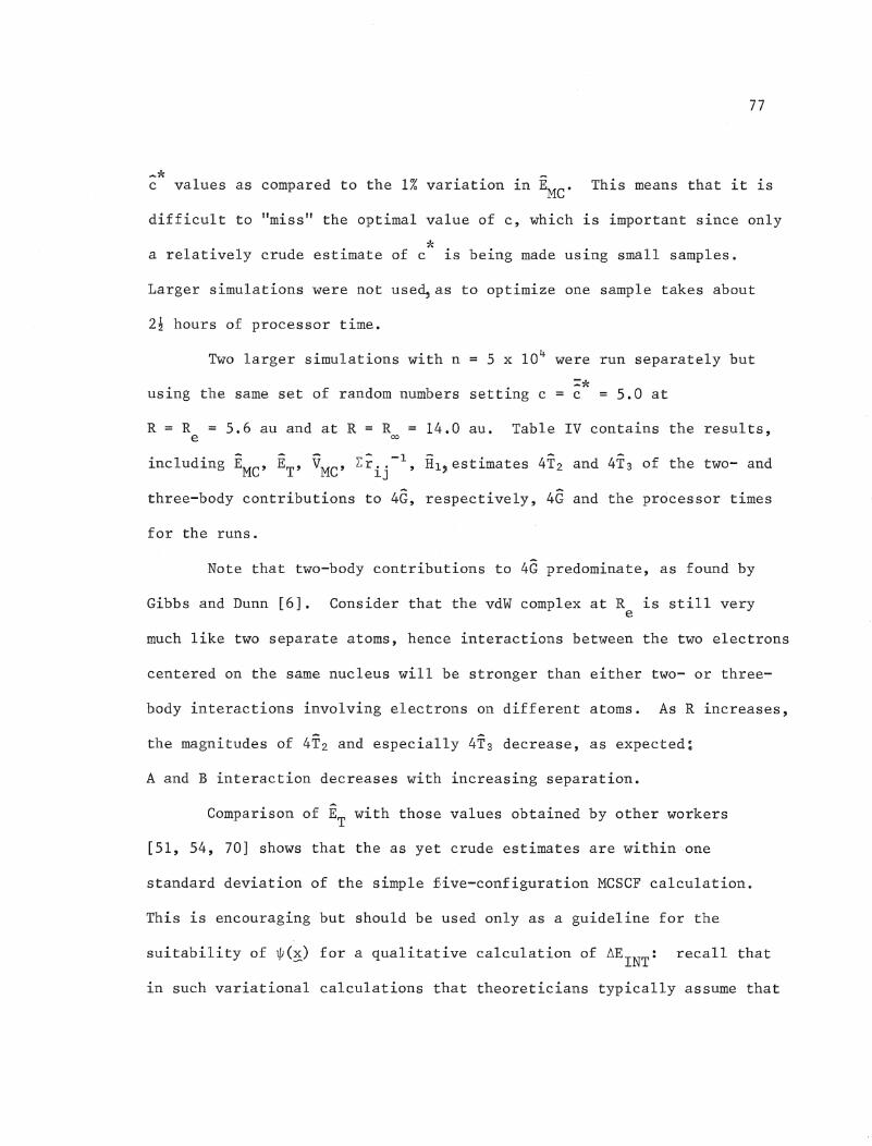
It should be noted that EMC

is not very sensitive to the value of

"'cc; a change in c in the vicinity of ~~ by one unit in either direction

only affects EMC in the third decimal place, hence the 20% variation in

*Parameter a should have in fact been set to -0.5 in order to obey thecusp condition.

76

TABLE III Optimization of a One-Parameter Correlated Wavefunction

for 1 + aLg He2 -

b -* cd eSample c ET EMC

1 4.83 -5.77 ± .05 -6.48 ± .05

2 4.35 -5.71 ± .06 -6.42 ± .06

3 4.83 -5.76 ± .05 -6.47 ± .05

4 5.24 -5.71 ± .06 -6.43 ± .06

5 4.18 -5.60 ± .09 -6.32 ± .09

6 6.50 -5.69 ± .07 -6.40 ± .07

7 4.06 -5.73 ± .05 -6.44 ± .05

8 4.16 -5.65 ± .08 -6.36 ± .08

9 4.76 -5.74 ± .05 -6.46 ± .05

10 6.57 -5.69 ± .07 -6.41 ± .07

Averages Computed from the Above Samples:

-:::::eJ~

C = 5.0 ± .9-ET. = -5.71 ± .05

-EMC -6.42 ± .05

a Trial wavefunction W(~) is given by (8.43); U(r .. ) from (11.2);-- --1J

~. from (9.5) with ~= 1.69; Cl, C2, E. for R = 5.6 au in Table II.1 1

b 3Separate samples of 10 Monte Carlo points.

c -*c estimates optimum c in U(r .. ) (11.2) which gives lowest E (8.34).~1J var

d ET

given by (10.3).

e -EMC given by (9.36).

77

_1<C values as compared to the 1% variation in E

MC• This means that it is

difficult to "miss" the optimal value of c, which is important since only

1<a relatively crude estimate of c is being made using small samples.

Larger simulations were not used,as to optimize one sample takes about

2! hours of processor time.

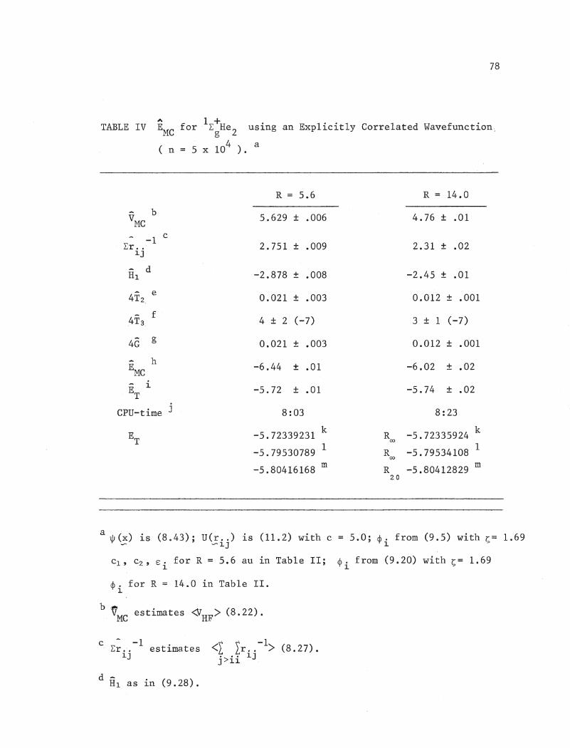
Two larger simulations with n = 5 x 104 were run separately but

=1<using the same set of random numbers setting c = c = 5.0 at

R = R = 5.6 au and at R = Re 0014.0 au. Table IV contains the results,

including EMC ' Er , VMC ' Lrij - 1, Hl,estimates 4T2 and 4Ts of the two- and

three-body contributions to 4G, respectively, 4G and the processor times

for the runs.

Note that two-body contributions to 4G predominate, as found by

Gibbs and Dunn [6]. Consider that the vdW complex at R is still verye

much like two separate atoms, hence interactions between the two electrons

centered on the same nucleus will be stronger than either two- or three-

body interactions involving electrons on different atoms. As R increases,

the magnitudes of 4T2 and especially 4T3 decrease, as expected:

A and B interaction decreases with increasing separation.

Comparison of Er with those values obtained by other ~rkers

[51, 54, 70] shows that the as yet crude estimates are within ,one

standard deviation of the simple Dive-configuration MCSCF calculation.

This is encouraging but should be used only as a guideline for the

suitability of ~(~) for a qualitative calculation of ~EINT: recall that

in such variational calculations that theoreticians typically assume that

78

A 1 +TABLE IV EMC for EgHeZ using an Explicitly Correlated Wavefunction

( n = 5 x 104 ). a

R = 5.6 R = 14.0

VMCb 5.629 ± .006 4.76 ± .01

.- -1 cL:r •. ' 2.751 ± .009 2.31 ± .02

~J

HId -2.878 ± .008 -2.45 ± .01

4T2e 0.021 ± .003 0.012 ± .001

4T3,f

4 ± 2 (-7) 3 ± 1 (-7)

4G g 0.021 ± .003 0.012 ± .001

- hEMC -6.44 ± .01 -6.02 ± .02

ET1- -5.72 ± .01 -5.74 ± .02

CPU-time J 8:03 8:23

ET -5.72339231 kR -5.72335924 k

00

-5.79530789 1R -5.79534108 1

00

-5.80416168 mR -5.80412829 m

20

a . .~(x) ~s (8.43); U(r .. ) is (11.2) with c = 5.0; ~. from (9.5) with ~= 1.69

........ "-~J ~

CI, C2' ci for R = 5.6 au in Table II; ~i from (9.20) with ~= 1.69

$. for R = 14~O in Table II.~

b ..VMC estimates <VHF> (8. 22) ·

c .- -1L:r .'. estimates

~J

d -HI as in (9.28)"

. . -1<I Ir .. > (8.27).• •• ~JJ>~~

see

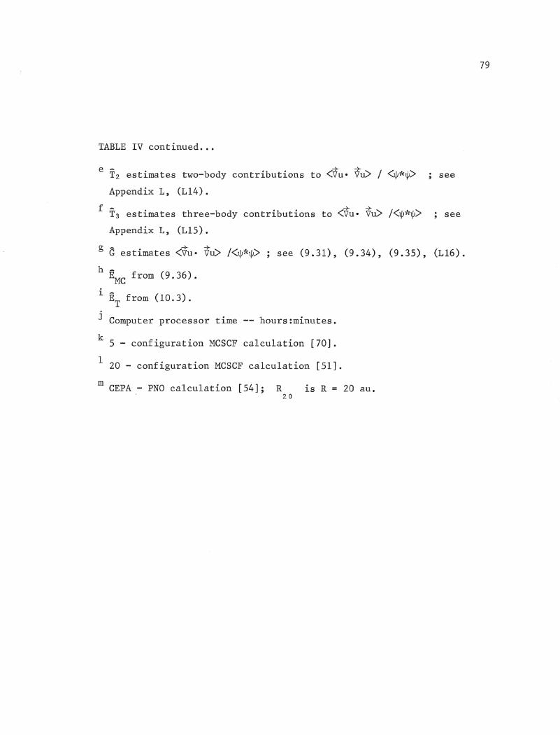
TABLE IV continued .•.

e- ~ +T2 estimates two-body contributions to <Vue \Ill> I <1/J1~1J;> see

Appendix L, (LI4).

f T3 estimates three-body contributions to <~u. Vll> 1<~*1/J>

Appendix L, (LI5).

79

g G estimates <~u e Vu> 1<1/J1<t/J>

h -EMC from (9.36).

i ET

from (l0. 3) .

see (9.31), (9.34), (9.35), (LI6).

j Computer processor time -- hours:minutes.

k 5 - configuration MCSCF calculation [70J.

1 20 - configuration MCSCF calculation [51J.

m CEPA - PNO calculation [54]; R is R = 20 au.20

80

the absolute error in E remains constant with R. The error in E isvar var

usually greater than the well-depth itself (Ch. VII).

Note that ET

values are not converging towards the more accurate

twenty-configuration MCSCF or CEPA-PNO result. It is apparent that this

sirilplle correlation function cannot recover all of the correlation energy.

The errors in the estimates ET are too large to calculate an

interaction energy. Even if correlated sampling had been used, it is

doubtful whether the reduction in variance would increase the accuracy in

the difference beyond the second decimal place. In order to obtain a

sample estimate of ET

accurate to the fifth decimal, it is estimated that

a sample on the order of 1010 would be needed. This would be an

extremely lengthy calculation given the processor time for a 5 x 10 4

calculation. It is felt that at this point, time would be more wisely

invested in making modifications to the existing programs in order to

make them more efficient. Such modifications are outlined below.

(i) The major time consuming element in the calculation involves the

probability inversion which finds ~. and n. for the configuration points1. 1.

(~(i», i 1, ••• , n. Other methods of generating random variables [29]

should be investigated on the basis of efficiency.

(ii) Simultaneous calculations at R = Rand R = R should be run,e 00

incorporating Correlated sampling (Ch. X), so that advantage is taken of the

variance reduction offered. In addition, other methods of variance

reduction, such as the use of control variates, should be exploited. A

reduction of variance of close to 50% has been obtained in Monte Carlo

simulations using this technique [38, 71].

81

(iii) An alternate method of Importance sampling for short and long R

may be more appropriate. It may be too much to expect one technique to

encompass the whole range of R (Appendix M: Note the different

transformations necessary in order to find n at short and long R.)

(iv) Incorporate Equations (9.27) for ~ .•1.

(v) General streamlining of FORTRAN code is desirable.

(vi) In the light of the footnote in "(XIa), the corrected form of (11.2)

should be used in the simulation.

(vii) In addition, the parameters were only optimized at R = 5.6 au.e

In practice they should be optimized at both internuclear separations.

energy.

82

XII. Discussion and Summary

The results permit only a short discussion on the suitability of

correlation functions (11.1) and (11.2). It was found that t/J(~)could

not be optimized with respect to one variational parameter, b, in

(11.1), while optimization with respect to c in (11.2) was possible.

Examination of the two functions shows that they behave quite differently

as functions of r ..• Since b in (11.1) is sent to very large values,1J

the correlation function tends towards a constant. This may mean that

large r .. values become too important in the optimization of this function.1J

The relaxation of the condition, a = 0.5,* and optimizing with respect to

a and b may allow t/J(~) using (11.1) to be optimized.

In vdW molecules most of the correlation energy arises from

interactions between electrons on different atoms and the intra-atomic

correlation energy remains essentially constant. Both (11.1) and (11.2)

are expected to deal with both inter- and intra-atomic correlation

A U(r .. ) which deals with the two effects separately would be~1J

more versatile.

The Basis Set Extension Effect was also not accounted for in these

calculations. Some technique, such as the use of ghost orbitals,

should be incorporated in order to avoid a fortuitous minimum.

In summary, in Part I of this work, theoretical derivations show

that in VMC calculations which employ the ratio estimate of E (4.8)var

* See footnote on p. 75.

83

have a bias of the estimate which is negligible for large samples (4.9).

Aside from the bias terms, the expected value of the estimate is the

variational energy (the exact energy plus terms second order in smallness

parameters (4.7)). The variance of the energy estimate is also second

order (4.13).

Given an infinite simple random sample, optimum variational

parameters obtained by minimizing the variance of the ratio estimate,

1<1<~ (4.15), are not identical to those which minimize the variational

,,;'<energy, ~ (4.14). This provides a theoretical explanation for the need

1<*to rescale after estimates of ~ are obtained.

For normalized wavefunctions, the VMC energy estimate (4.17) is

unbiased; it has E for its expected value (4.18). However, for largevar

samples, the biased ratio estimator is preferred because it has a smaller

variance due to the correlation of two random variables, H (4.3) and S

(4.4). The theoretical result given in (4.19) shows that the unbiased

estimate has a variance which is zeroth order in smallness parameters.

A numerical example using Importance sampling and a Hylleraas

variational wavefunction for 1 IS He is given. The results indicate that

there is no advantage to using minimization of the variance as a

parameter optimization scheme.

The diffusion Monte Carlo energy estimate of Reynolds et ale [25]

has negligible bias for large t (5.14). (It is assumed that the nodes

of the exact wavefunction correspond exactly to those of the guiding

function.) The estimate yields the exact energy in the limit of

84

infinite t. However, the variance of the energy estimate is second order

in smallness parameters, even at infinite t (5.15c). This provides a

theoretical justification for the empirical observation that the

precision of DMC calculations is strongly dependent on the choice of the

guiding function.

In Part II, it is shown that a partitioned form of the Hamiltonian

(8.24) can be used in conjunction with an explicitly correlated wave-

function (8.28), which allows E to be expressed by a combination ofvar

HF-SCF results and terms involving the gradient of the correlation

function (8.34).

Equations are derived which allow the Hartree-Fock potential, VHF

(8.14), expressed in terms of coulomb and exchange operators, to be applied

to an explicitly correlated wavefunction for the vdW molecule, He2. A

method of Importance sampling in prolate spheroidal coordinates is

derived. A VMC calculation is performed for He2' firstly for the HF-SCF

wavefunction and secondly for an explicitly correlated wavefunction. The

latter employs results of Part I to optimize ¢(~.) for one form of U(r .. )~. ~1.J

(11.2). A wavefunction using another correlation function (11.1) could

not be optimized. Although the Monte Carlo estimates at short and long

distances agree within statistical error with representative

(qualitative) MCSCF results, it is not possible to estimate ~EINT because

of insufficiently accurate values of EMC • Modifications which could

allow the computer program to run more efficiently are discussed.

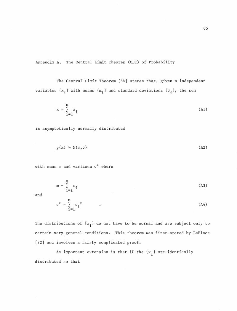
85

Appendix A. The Central Limit Theorem (CLT) of Probability

The Central Limit Theorem [34] states that, given n independent

variables {x.} with means {m.} and standard deviations {a.}, the sum111

n

x = L x.i=1 1

is asymptotically normally distributed

p(x) ~ N(m,a)

with mean m and variance a 2 where

(AI)

(A2)

and

mnI m.i=1 1

n

I a. 2

i=1 1

(A3)

(A4)

The distributions of {x.} do not have to be normal and are sufiject only to1

certain very general conditions. This theorem was first stated by LaPlace

[72] and involves a fairly complicated proof.

An important extension is that if the {x.} are identically1

distributed so that

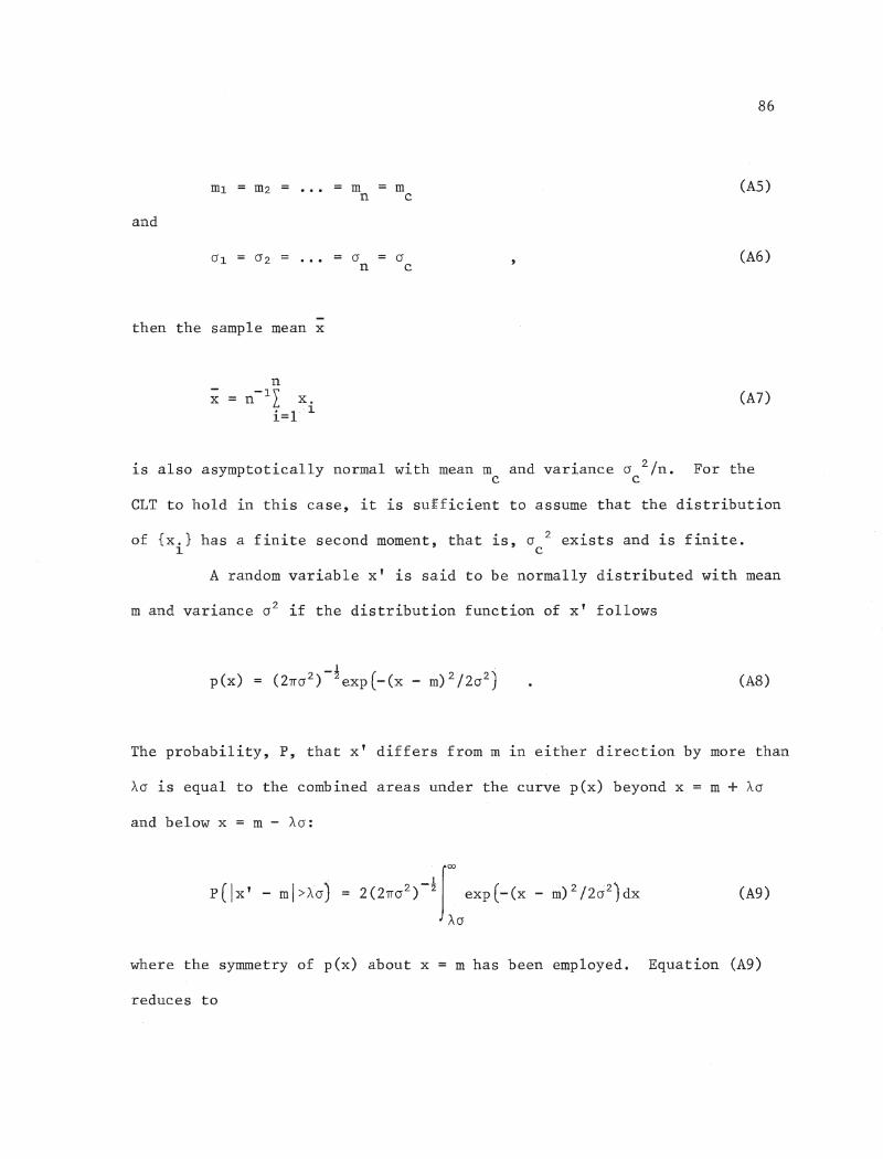
and

m = mn c

86

(AS)

then the sample mean x

nx = n-1I x.

i=l \.1.

on

oc

(A6)

(A7)

is also asymptotically normal with mean m and variance 0 2/n • For thec c

eLT to hold in this case, it is sufficient to assume that the distribution

of {x.} has a finite second moment, that is, 0 2 exists and is finite.1 c

A random variable x' is said to be normally distributed with mean

m and variance 02 if the distribution function of x' follows

p(x)I .

(2n02)-2 exp (_(x - m)2/ 2cr2) (AB)

The probability, P, that x' differs from m in either direction by more than

AO is equal to the combined areas under the curve p(x) beyond x = m + AO

and below x = m - AO:

p(lx' - rnl>Acr) = 2(2'lfcr2)-~JOO exp(-{x - rn)2/ 2cr2)dxAO

(A9)

where the symmetry of p(x) about x

reduces to

m has been employed. Equation (A9)

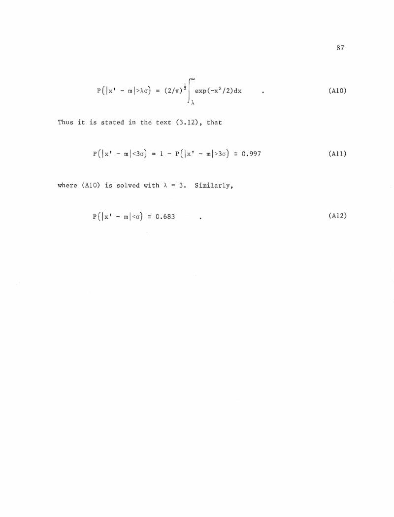
Thus it is stated in the text (3.12), that

87

(AID)

P ( Ix' - mI<30) 1 - p(/x' - ml>3a) - 0.997 (All)

where (AID) is solved with A 3. Similarly,

p(lx' - ml<a) - 0.683 (AI2)

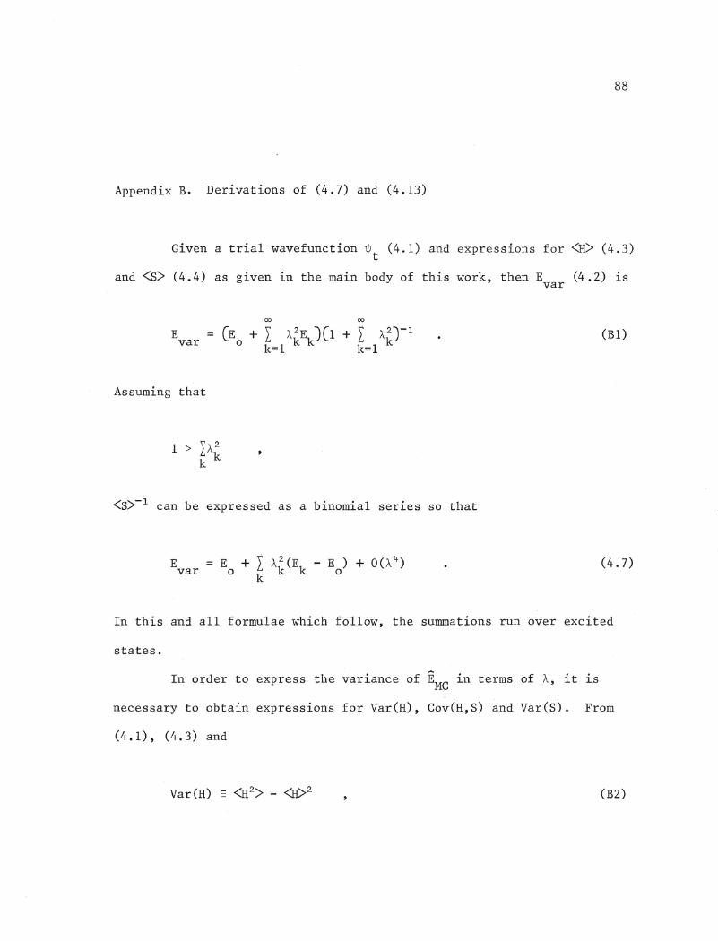
88

Appendix B. Derivations of (4.7) and (4.13)

Given a trial wavefunction ~ (4.1) and expressions for <H> (4.3)t

and <8> (4.4) as given in the main body of this work, then E (4.2) isvar

00 00

Evar

Assuming that

(Bl)

<8>-1 can be expressed as a binomial series so that

Evar(4.7)

In this and all formulae which follow, the summations run over excited

states.

In order to express the variance of EMC in terms of A, it is

necessary to obtain expressions for Var(H) , Cov(H,8) and Var(S)~ From

(4 •1), (4 •3) and

(B2)

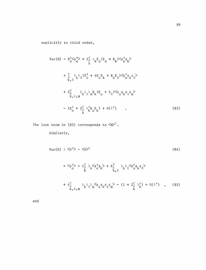
explicitly to third order,

+ ~ iAkAi(E~ + 4EoEk + EkEi)<~~~k~i>,

The last term in (B3) corresponds to <H>2.

Similarly,

89

(B3)

(B4)

and

Cov(H,S) = <HS> - <H> <S>

+ 3~ ~AkA~(Ek + EO)<~~~k~~>,

+ 2 AkAnA (E + 3Ek)<¢ ¢k¢n¢ >k n ~ ~ moo ~ m, ~,m

The variance of the ratio estimate, Var(EMC)' ~s given by,

90

(B6)

(B7)

(4.10)

where 0(n- 2) reflects the bias. After substituting (4.6), (4.7), (B3),

(B5) and (B7) into (4.10), all zero and first-order terms in A drop out,

leaving

Var(EMC) = n-1(1 + ~ A~)-2[~ ~ AkA~(Ek - Eo)(E~ - Eo)<~~~k~~>,

+ 2I AkAnA (Ek - E )(E - E )<¢ ¢k¢n¢ > + 0(A 4 »). (B8)k n ~ mom 0 0 ~ m,~,m

91

Expanding (1 + L A~J-2 as a binomial series and multiplying out leavesk

(4.13)

where only second order terms have been written out explicitly.

If Importance sampling has been used, then the corresponding

equations for (4.3) and (4.4) are

(B9)

(BIO)

where p is a normalized and everywhere non-negative probability density (3.3).

The equations for E (4.2) and Var(EMC ) (4.10) still hold but where Iivar

(B9) and S (BI0) replace H (4.3) and S (4.4), respectively. Hence, using

the expansion in smallness parameters,

<H> = Eo<~~/P> + I Ak(Eo + Ek)<~o~k/P> + I ~AkA~Ek<~k~~/P> (BII),

<5> = <~~/P> + 2I Ak<~o~k/P> + I ,/kA~<~k~~/P> (BI2),

which reduce to

92

<if> <If> = E + I A~Ek0k

<3> = <8> 1 + I A2

kk

(B13)

(B14)

Hence the use of Importance sampling does not affect the expectation values

and (4.7) holds for Evar

The Var(EMC) for importance sampling is, after finding Var(H) ,

Var(S), Cov(H,S) for use in an analogous expression to (4.10) is

(B15)

The difference between (B15) and (4.13) to second order is the existence

of the p2 term in the denominator of the expectation value. Importance

sampling does alter Var(EMC), however it is of note that (B15) is second

order in Ae

93

Appendix C~ Derivation of (4~19)

Given a normalized trial wavefunction, $t (4.16), the variational

energy, using (4.16) in (4.3), is

E - <II>var

00

(C1)

where a binomial expansion of <S>-l has been used. The variance of the

Monte Carlo estimate is

(C2)

After substituting (4.3) and (4.16) and then expanding in terms of A,

n-l[E~C<~~> - 1) + zr=l AkEo(Eo + Ek)<~~~k> + O(A2)]

(4.19)

where terms of second and higher order in A are implicit.

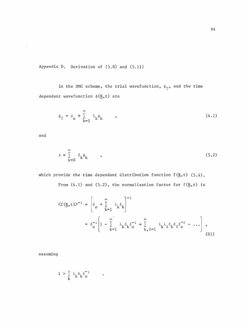
Appendix D. Derivation of (5.8) and (5.11)

In the DMC scheme, the trial wavefunction, ~T' and the time

dependent wavefunction ~(~,t) are

00

<Po + I Ak<Pkk=l

and

00

94

(4.1)

(5.2)

which provide the time dependent distribution function f(~,t) (5.4).

From (4.1) and (5.2), the normalization factor for f(g,t) is

[0

0+ I AkOkJ-l

k=l

0~1[1 - k~-~l AkOko~l + I AkAlOkOlo~2 - ••• Jk,.Q,=l

assuming

(D1)

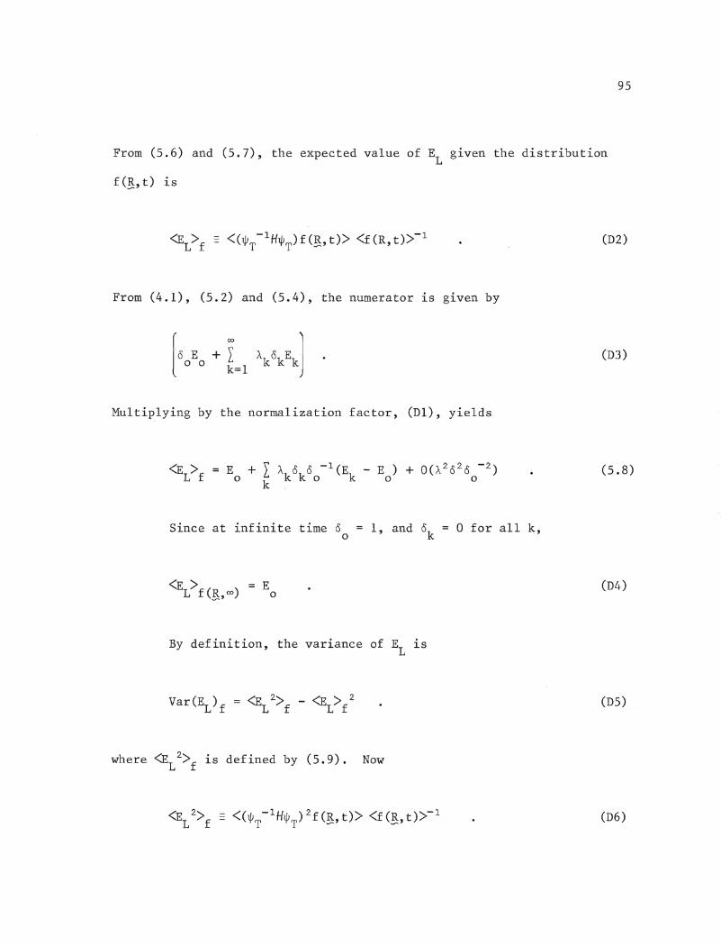
95

From (5.6) and (5.7), the expected value of EL

given the distribution

f(~,t) is

(D2)

From (4.1), (5.2) and (5.4), the numerator is given by

(D3)

Multiplying by the normalization factor, (D1), yields

(5.8)

Since at infinite time 0o

1, and ok 0 for all k,

(D4)

By definition, the variance of EL

is

where <EL2>f is defined by (5.9). Now

(D6)

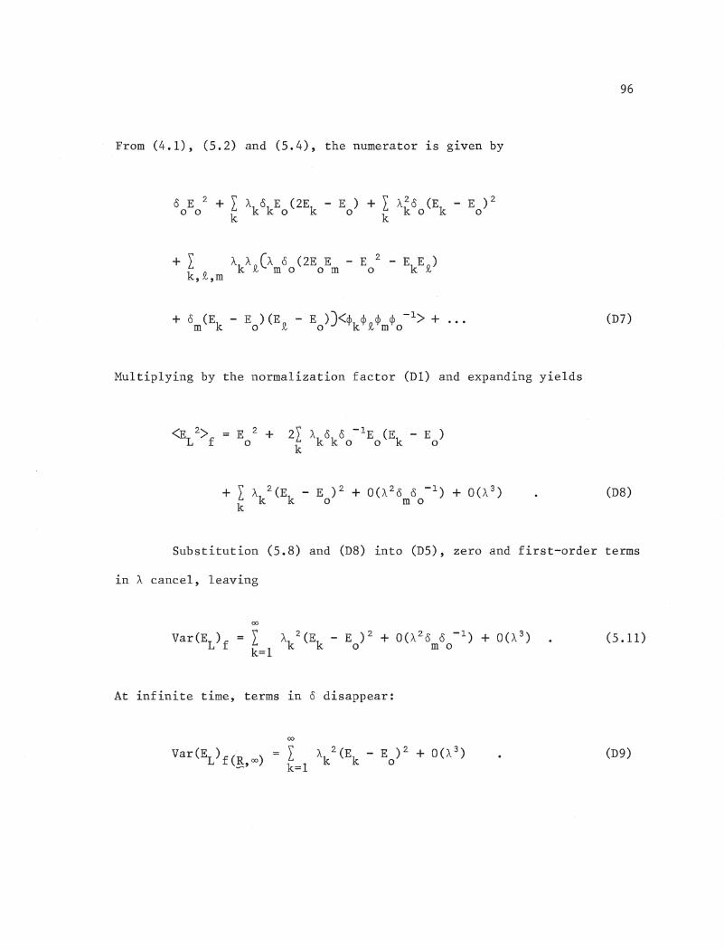
96

From (4.1), (5.2) and (5.4), the numerator is given by

+ I ~k~nC~ 8 (2E E - E 2 - EkE n)Yv moo m 0 N

k, ~,m

+ 8 (Ek - E )(E n - E ))<¢k¢n¢ ¢ -1> + ...m 0 Yv 0 . Yv m 0

Multiplying by the normalization factor (Dl) and expanding yields

(D7)

E 2 +o

(D8)

Substitution (5.8) and (D8) into (D5), zero and first-order terms

in ~ cancel, leaving

00

= Ik=l

(5.11)

At infinite time, terms in 8 disappear:

00

Ik=l

(D9)

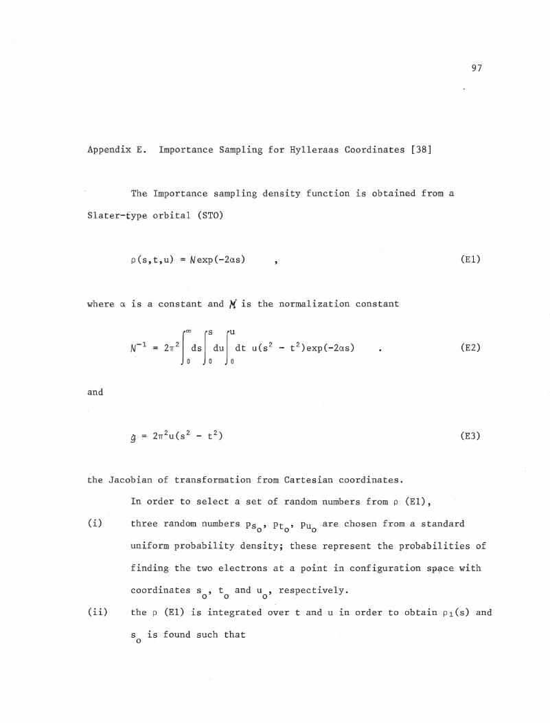
97

Appendix E. Importance Sampling for Hylleraas Coordinates [38]

The Importance sampling density function is obtained from a

Slater-type orbital (STD)

p(s,t,u) = Nexp(-2as)

where a is a constant and H is the normalization constant

and

the Jacobian of transformation from Cartesian coordinates.

In order to select a set of random numbers from p (El),

(El)

(E2)

(E3)

(i) three randolffi numbers PSe' Pte' PUo are chosen from a standard

uniform probability density; these represent the probabilities of

finding the two electrons at a point in configuration sp~ce with

coordinates so' t and u , respectively.o 0

(ii) the p (El) is integrated over t and u in order to obtain Pl(S) and

S 1S found such thato

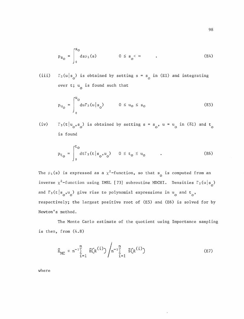
o ~ s < 00

o

98

(E4)

(iii) r 2(u\s ) is obtained by setting so

over t· u is found such that, 0

s in (El) and integratingo

J

u o

Pu = dur 2(uls)o 0

o

(E5)

(iv) r 3(tlu ,s ) is obtained by setting so 0

is found

so' u = uo in (.El) and to

J

t o

dtr3(tls ,u )o 0

o(E6)

The Pl(S) is expressed as a X2-function, so that s is computed from ano

inverse x2-function using IMSL [73] subroutine MDCHI. Densities r 2(u\s )o

and r3(tls ,u ) give rise to polynomial expressions in u and t ,o 0 0 0

respectively; the largest positive root of (E5) and (E6) is solved for by

Newton's method.

The Monte Carlo estimate of the quotient using Importance sampling

is then, from (4.8)

n_n-1l: ii(R(i))i=l

where

n

Li=l

(E7)

99

(E8)

where 9 1S given by (E3).

The corresponding estimate of the variance of EMC is from (4.10)

-Var(E

MC) - (nS 2 )-1(Var(H) (E10)

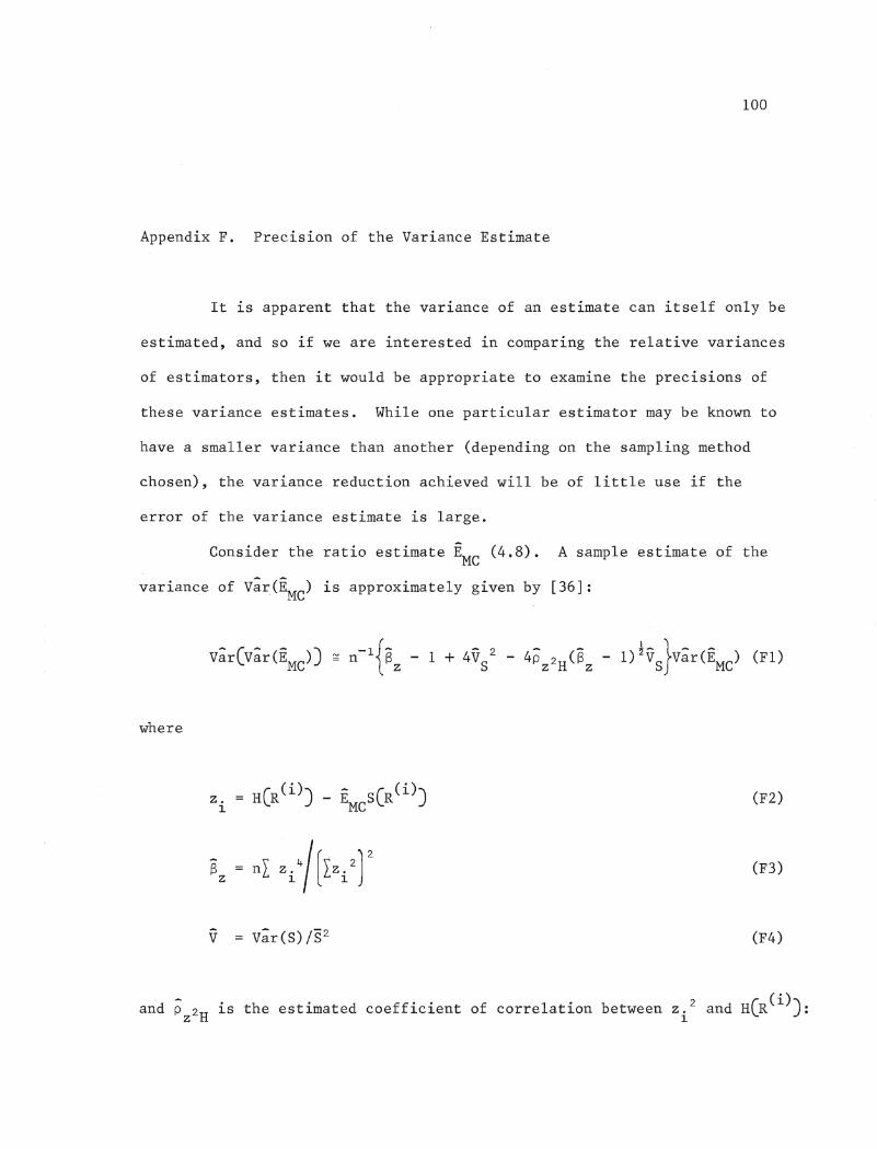
100

Appendix F. Precision of the Variance Estimate

It is apparent that the variance of an estimate can itself only be

estimated, and so if we are interested in comparing the relative variances

of estimators, then it would be appropriate to examine the precisions of

these variance estimates. While one particular estimator may be known to

have a smaller variance than another (depending on the sampling method

chosen), the variance reduction achieved will be of little use if the

error of the variance estimate is large.

Consider the ratio estimate EMC (4.8). A sample estimate of the

variance of Vir(EMC ) is approximately given by [36]:

where

z. H(R(i») - E S(R(i») (F2)1 Me

Sz nI z. [Iz/f (F3)1

V Vir(S)/S2 (F4)

and p is the estimated coefficient of correlation between z.2 and H(R(i)):z2H 1 .

101

The square root of (Fl) is used to create one standard deviation

error bars on the estimated variance of EMC

.

102

Appendix G.

Derivation of (8.19)

From the ,',definition of HTOT (8.13)HF

N NI H. + I L (J.. - K•• )i=l ~ j;zti i=l ~J 1.J

Using ~(~) (8.15) to evaluate the expectation value

(G1)

N= I <~(~) IHil~(~»

i=l

N+ I L <~(x)IJ·· - K.. I~(x»

j7i i=l ~ 1.J ~J ~(G2)

Appendix C in Blinder [56] shows that

NI <<p. IH. I<P .>i=l ~ ~ ~

The second step in (G3) comes about by the properties of A and the symmetry

of the H. operator with respect to the electron coordinates.~

The operators J .. (8.8) and K•• (8.9) do not affect the spin~J 1.J

coordinates and are symmetrical with respect to the spatial coordinates.

103

Hence,

NI I <~(x) IJ .. - K•• I~(x»j7i i=1 ~ 1J 1J ~

= I I J ••• JdXl ••• dXN~~(I) ••• ~N*(N)(J.. - K•• )· · · 1 - 1J 1J]7:1 1=

N!x I (-1)rPr• 1 (1) .•.•N(N)

r=1(G4)

Only the permutations involving electrons i and J will contribute

non-zero integrals and so the above can be written as

I I J.. . JdXl ••• dxN~~(l).•• ·~N1<{N) JdX,<p~(X')r. -1 •. (X')· · · 1 J 1X JJ 7:1 1=

- J,dx ' <P \ x ' )r. -1 P " · ~ · (x ') <P 1 ( 1) ••• [ <P • (i) ~ . (j) - ~. (i) ~ · (j ) ]J 1X1J J 1 J J 1

(G5)

Carrying out the operations and separating the integrals leads

to

N

I Ij ·~i i=l

104

I *. II * *dXl¢l(l)¢l(l) ... .. dx.dx'¢.(i)¢.(x')r. -l¢.(i)¢.(x')1. 1. J 1.X 1. J

- I ~ Idx1 ¢~ ( 1) ¢ 1 ( 1) ..• I·· Idx .* dx ' ~ 1~ ( i) ep 1:. (x ' ) r _ -1 ep • (i) ep .- (x ')j 7i i =1 1. 1. J 1.X J J

(G6)

But cp. and cp. are orthonormal, so second and fourth terms disappear,1. J

leaving

L I IIdX.dX'~~(i)~~(X')r. -l~.(i)~.(x')j;ei i=l 1. 1. J 1.X 1. .J

II * * -1- dx.dx'~.(i)~.(x')r. ~.(i)~.(x')1. 1. . J 1.X J 1.

N= I I (J .. - K .. )

j;2ti i =1 1.) 1)

Combining (G2), (G3) and (G7) gives

. TOT' ~ . N'<ep (2f) f HHF Iep (~)> = I <~ · IH. I¢ ·> + I I (J .. - K. • )

· 1 1 1 1. •.•• 1 1.) 1)1.= J 7:1 1.=

105

(G7)

(8.19)

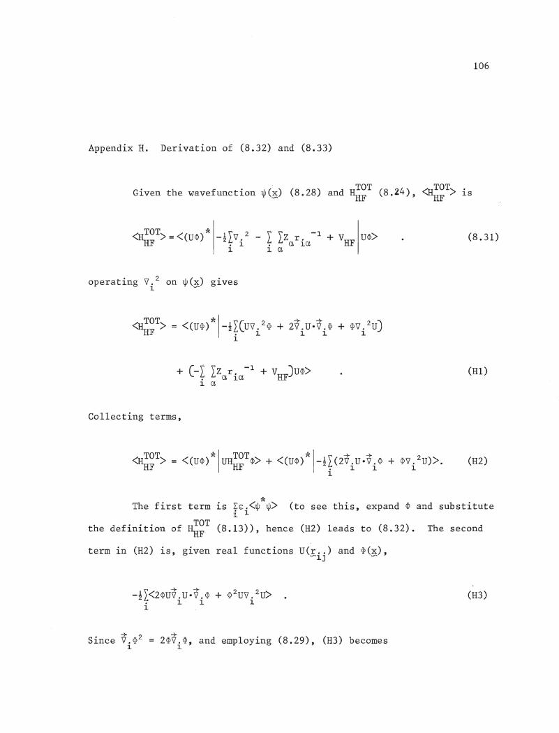
106

Appendix H. Derivation of (8.32) and (8.33)

Given the wavefunction W(~) (8.28) and HTOT (8.24), <HTOT> is-- HF HF

(8.31)

operating V. 2 on W(~) gives1.

~~T> = «U<P)*I-!fCuvi2<P + 2ViUoVi<P + <pv/u)1

+ (-I Iz r. -1 + VHF)U~>• Cl 1Cl1. Cl

Collecting terms,

(HI)

~~T> = «U<P)*lu~~T<p> + «U<P)*I-!f(2ViUO~i<P + <pv i2U». (H2)

1

The first term is fE i <$*$> (to see this, expand <p and substitute:k.

the definition of H~~T (8.13)), hence (H2) leads to (8.32). The second

term in (H2) is, given real functions U(r .. ) and ~(~),.......1J --

(H3)

-+2~V.~, and employing (8.29), (H3) becomes

1

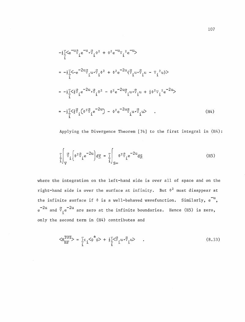
107

\ -u+ -u + 2 2 -u 2-U-~L<e V.e ·V.@ + @e V. e >.11 11

(H4)

Applying the Divergence Theorem [74] to the first integral in (H4):

(H5)

where the integration on the left-hand side is over all of space and on the

right-hand side is over the surface at infinity. But @2 must disappear at

the infinite surface if ~ is a well-behaved wavefunction. Similarly, e-u ,

-2u + -2ue and V.e are zero at the infinite boundaries. Hence (H5) is zero,1

only the second term in (H4) contributes and

(8.33)

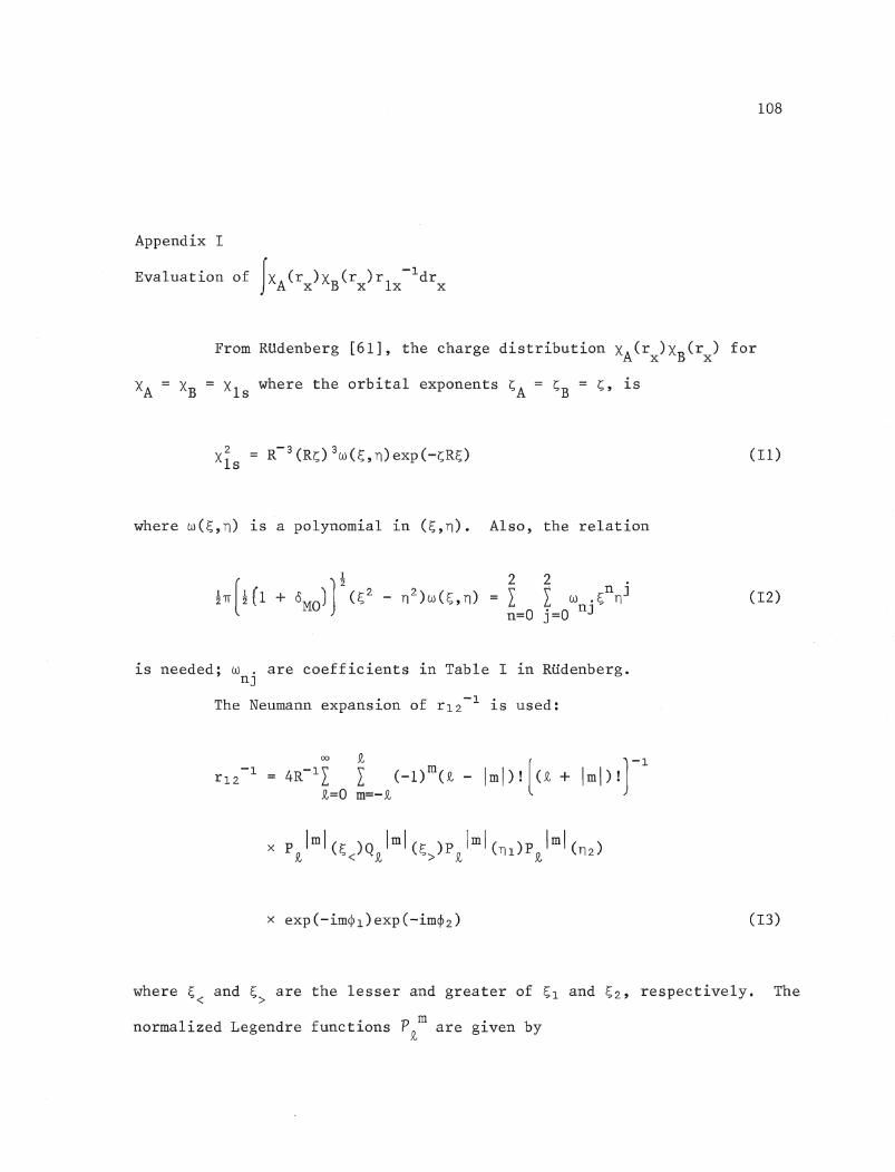
108

Appendix I

Evaluation of IXACrX)XBCrX)rlX-ldrX

From RUdenberg [61], the charge distribution xA(rx)xB(rx) for

XA XB = XIs where the orbital exponents ~A = ~B = ~, is

where w(~,n) 1S a polynomial in (~,n). Also, the relation

(II)

I

h(Hl+ 0Mo)fC!;2 - n2)wC!;,n) (12)

is needed; w . are coefficients in Table I in RUdenberg.nJ

The Neumann expansion of rlZ- 1 is used:

(13)

where ~ and ~ are the lesser and greater of ~1 and ~z, respectively. The< >

normalized Legendre functions P m are given by~

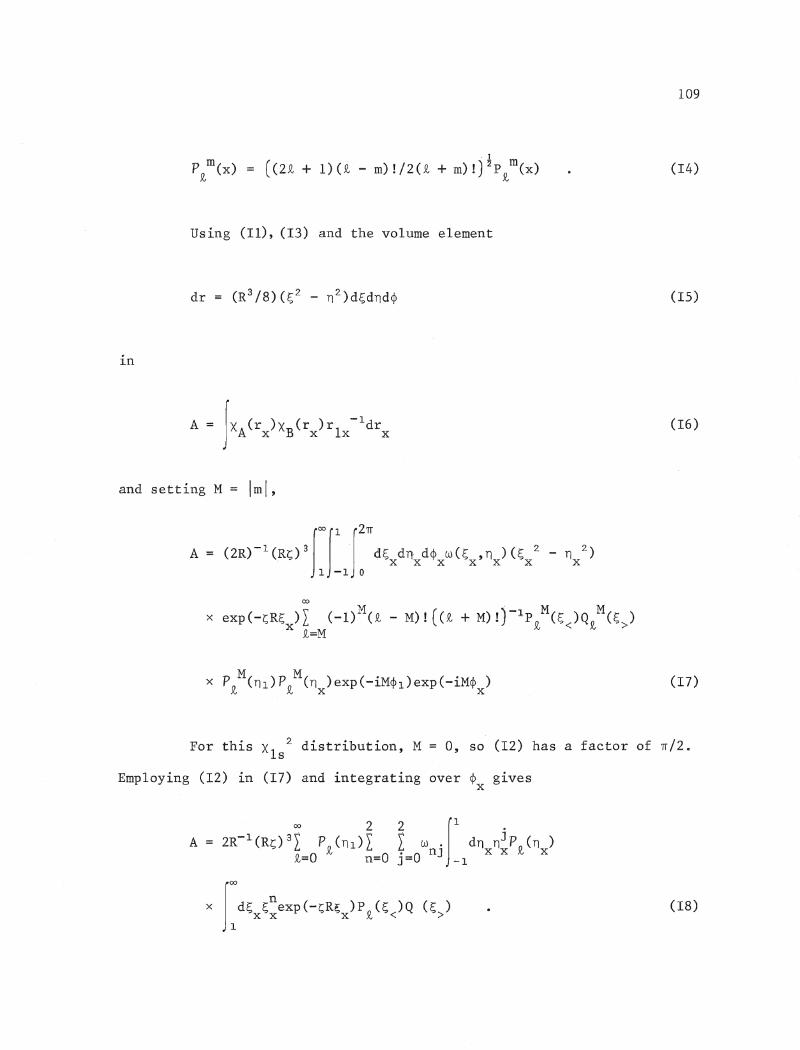
· I

((2£ + 1)(£ - m)I/2(£ + m)I)2 P£m(x)

109

(14)

Using (II), (13) and the volume element

in

and setting M = Iml,

00

x exp(-~R~x)I (_l)M(£ - M)l((£ + M)!)-lP£M(~<)Q£M(~»~=M

(15)

(16)

(17)

For this X1s

2 distribution, M = 0, so (12) has a factor of ~/2.

Employing (12) in (17) and integrating over ¢x gives

(18)

110

Substitute B?i(O) (9.13) for the integral over n. Rearrange theJ x

integral over ~ so thatx

A00 2 2. .. Oi

2R-1 (Rs)3I P2(nl)I I W .BJ. (0)

i=O n=O j=O nJ

x Q2(~1) J:ld~x~xneXP(-sR~x)P2(~X)

+ PO(~l)Joo d~ ~ nexp(-sR~ )Qn(~ )N X X X N X

~l

(19)

From the definitions of Kin(~l,a) (9.11) and Lin(~l,a) (9.12) and p~ (14),

(19) becomes

A

(9.10)

O~Following the expansion of B. (0) and values of w • given by RUdenberg,J nJ

only i = 0,2 terms are non-zero in (9.10)~ Appendices Band D in Harris

[75] provide recursion formulae for Po m, On ill, Ko m and L o ffi. In thisNil .. Nn Nil Nil

m m m.. mwork, P~n ' Q~n ,Kin were found uS1ng these formulae; the L~n were found

using the explicit formula for L80, a 24-point Gauss-Laguerre quadrature

1 mfor L~O and recursion formulae for other L~n •

111

Appendix J.

Terms Arising From (9.19)

(a) Short R, where (9.5) holds

Using (9.7) and (9.8) as definitions of ]., and the shortened~

notations

[1234] <PI (1) <P2 (2) <1>3 (3) <P4 (4)

[1432] <PI (1) <P4 (2) <P3 (3) ¢2 (4)

[3214] ¢3 (1) $2 (2) <PI (3) <P4 (4)

[3412] ¢3(1)<P4(2)¢1(3)¢2(4)

(J1a)

(JIb)

(J1c)

(J1d)

where the (ordered) electrons, 1, ... , 4 are in orbitals designated by the

numbers in square brackets, then

4I J. ([1234] - [1432] - [3214] + [3412])i=l ~

(J2)

Using similar notation to (J1), (9.15)-(9.18) for K.<p. and the~ ~

symbol

(9.15)

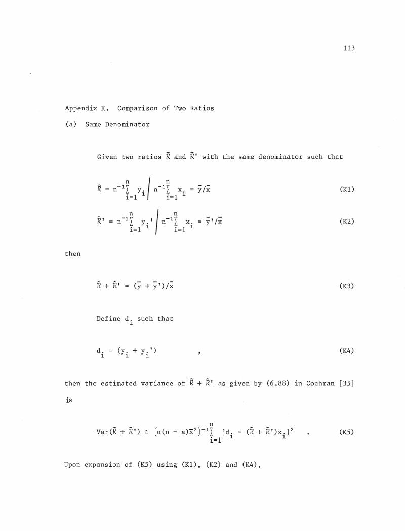
113

Appendix K. Comparison of Two Ratios

(a) Same Denominator

Given two ratios Rand R' with the same denominator such that

then

(Kl)

(K2)

(y + y') j;' (K3)

Define d. such that1

d.1

(y. + y. ')1 1

(K4)

then the estimated variance of R+ R' as given by (6.88) in Cochran [35]

is

(K5)

Upon expansion of (K5) using (Kl), (K2) and (K4),

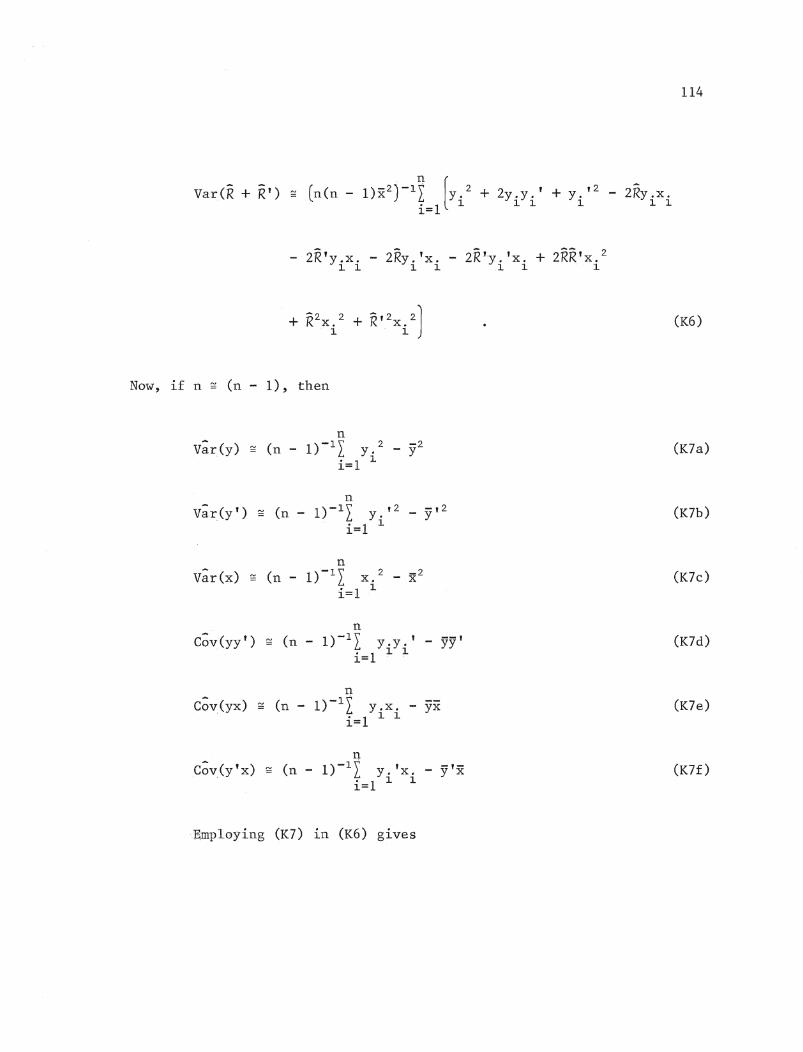
- 2R'y .. x .. - 2Ry .. 'x. - 2R'y. 'x. + 2RR'x. 21. ~ 1. 1. ',~ ~ '1.

114

Now, if n - (n - 1), then

(K6)

V~r(y)

n_ (n - I)-II y. ,2 _ y,2

i=1 ~

(K7a)

(K7b)

vir (x)n

_ (n - I)-II x. 2

i=l ~

-2- x (K7c)

C~v(yy')n

- (n - I)-II y .. y.' - yy'i=I 1. 1.

n- (n - 1)-Ir y .. x .. - yx

i=1 ~ 1.

n- (n - l)-IL y. 'x. - y'x

i=1 1. 1.

(K7d)

(K7e)

(K7f)

:mmploying (K7) in (K6) gives

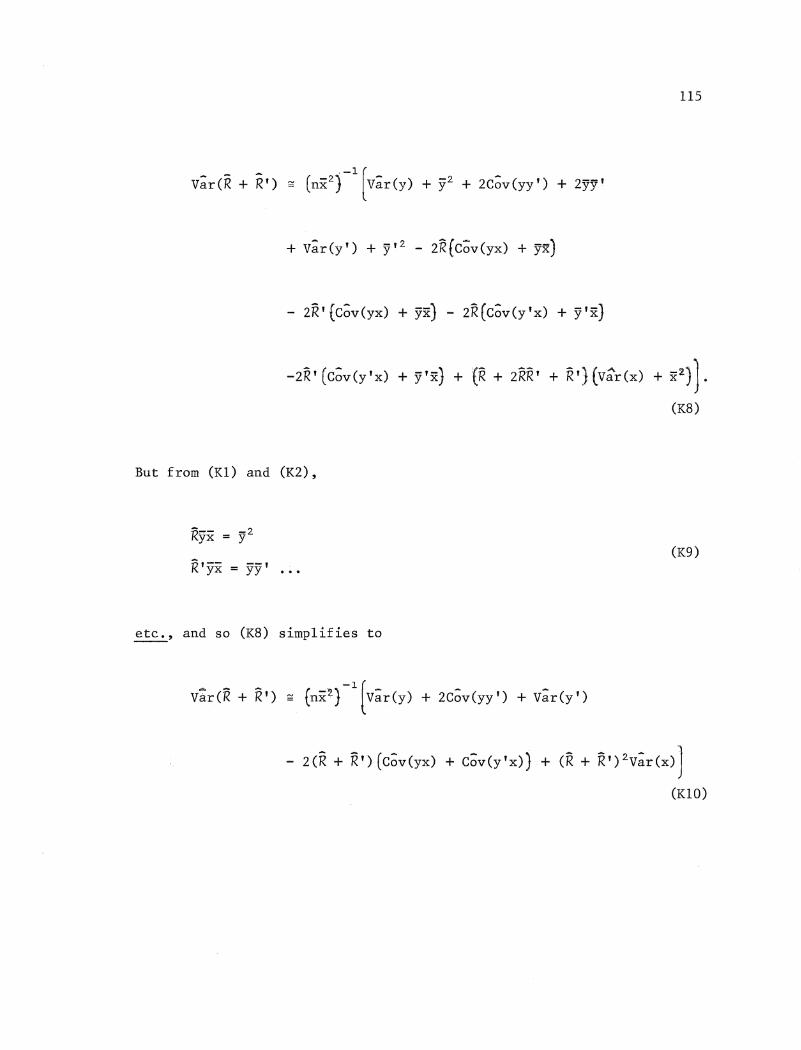
115

+ V~r(y') + y,2 - 2R(Cov(yx) + yx)

-2R' (C~v(y'x) + Y"x) +(R + 2RR' + R').{V~r(x) + x2j).(K8)

But from (Kl) and (K2),

R'yx = yy'

etc., and so (K8) simplifies to

(K9)

- 2(R + R')(C~v(yx) + C~v(y'x) + (R + R,)2V;r(x)]

(KID)

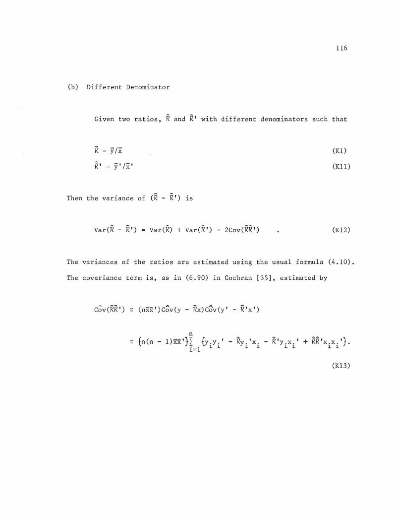
116

(b) Different Denominator

Given two ratios, Rand R' with different denominators such that

R= y/x

R' = y' /x'

Then the variance of (R R') is

(Kl)

(K11)

(K12)

The variances of the ratios are estimated using the usual formula (4.10).

The covariance term is, as in (6.90) in Cochran [35], estimated by

n_ (n(n - l)xx'}I ty.y.' -- Ry. 'x.

i=1 1 1 1 1R. 'y .x.' + RR 'x .x. ') •

1 1 1 1

(K13)

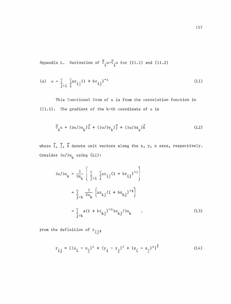
Appendix L. -+ -+Derivation of V.u-V.u for (11.1) and (11.2)1. 1.

117

(a) u = I Iar .. (1 + br .. )-1j >i i 1.J 1.J

(Ll)

This functional form of u is from the correlation function in

(11.1). The gradient of the k-th coordinate of u is

(L2)

-r -r -+ • 1 " 1where 1., J, k denote un1.t vectors a ong the x, y, x axes, respect1.ve y.

Consider dU/dXk

using (Ll):

[~ . Iar .. (l + br .. ) -11

J·.

• • • 1.J 1.JJ>1. 1.

(L3)

From the definition of r .. J1.J

r ..1.J

1[(x. - x.)2 + (y. - y.)2 + (z. _ Z.)2]2

1. J 1. J 1. J(L4)

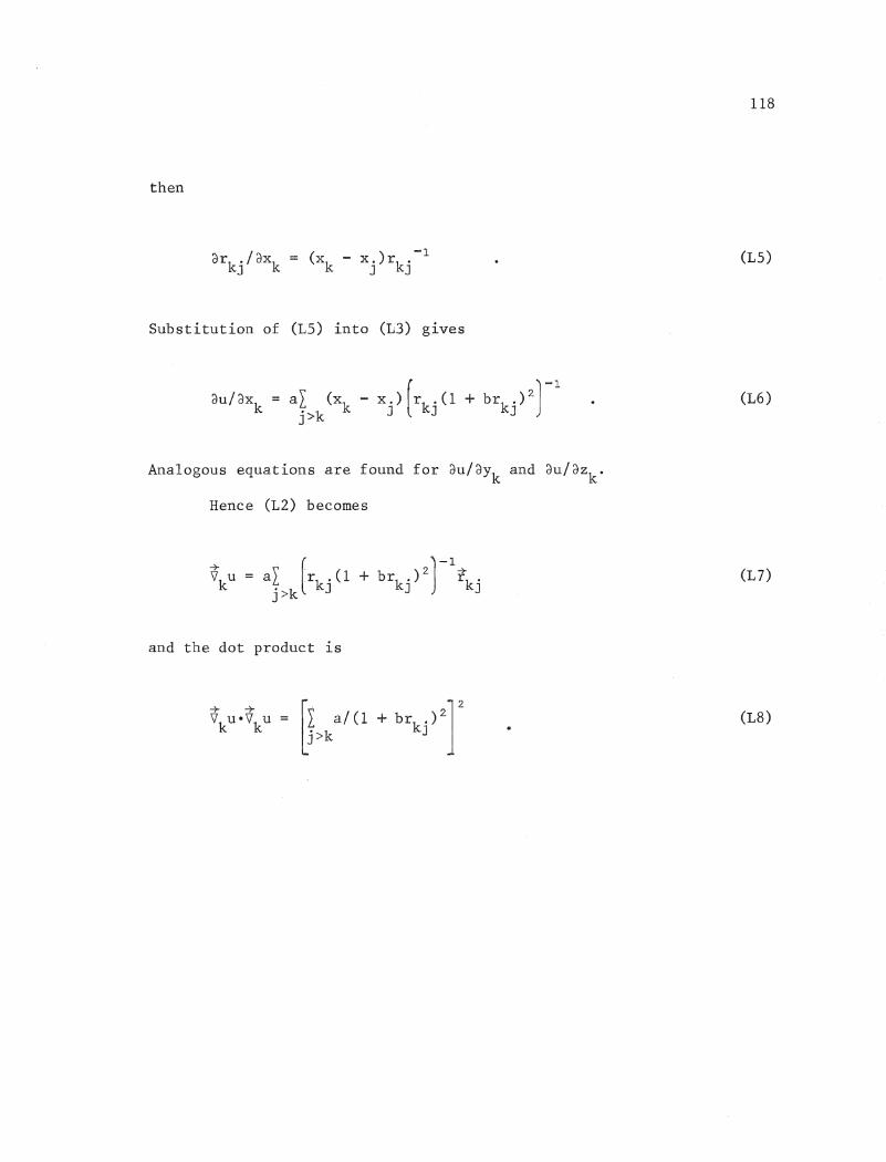
then

118

(L5)

Substitution of (L5) into (L3) gives

Analogous equations are found for dU/dYk and dU/dZke

Hence (L2) becomes

and the dot product is

(L6)

(L7)

(L8)

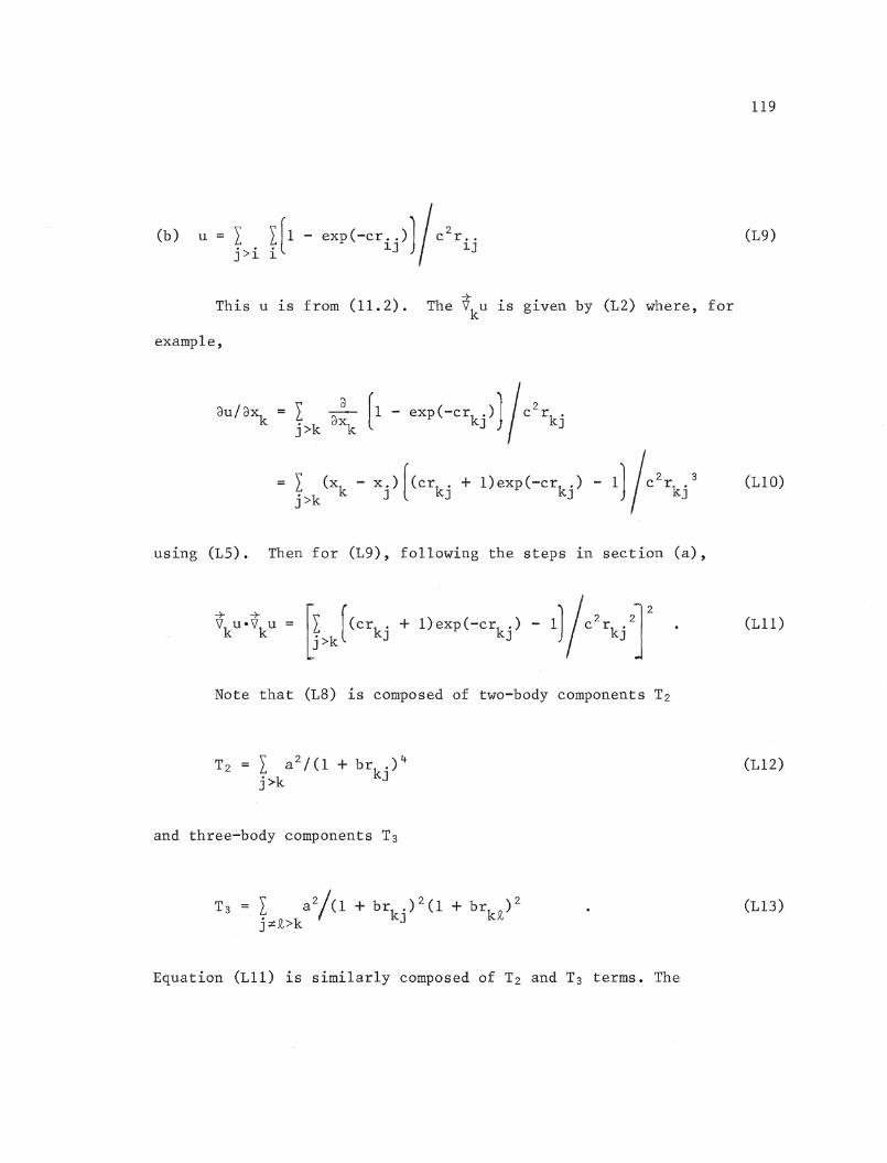
(b) u = I I[l - exp(-cr .. )j >i i ~J

This u is from (11.2).

example,

-+The Vku is given by (L2) where, for

119

(L9)

L d~k [1 - exp(-crkj ))·j>k

L (xk - x.)(crk · + l)exp(-crkJ

·) - 1)j>k J J

2 r skj

(L10)

using (L5). Then for (L9), following the steps in section (a),

(Ll1)

Note that (L8) is composed of two-body components T2

and three-body components Ts

Equation (Ll1) is similarly composed of T2 and Ts terms. The

(LI2)

(L13)

calculation estimates

+ + -J~= <Vu e Vu>/<1jJ 1jJ>

where 1jJ 18 the correlated wavefunction.

120

(L14)

(LIS)

(L16)

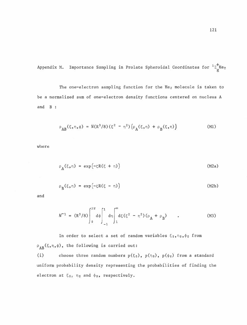
Appendix M.

121

Importance Sampling in Prolate Spheroidal Coordinates for IL+He2g

The one-electron sampling function for the He2 molecule is taken to

be a normalized sum of one-electron density functions centered on nucleus A

and B:

(M1)

where

and

J

2TI JI JOON- 1

= (R3 /8)0 d~ dn Id~(~2 - n2)(PA + PB)

-1

In order to select a set of random variables ~o,no,¢o from

(M2a)

(M2b)

(M3)

PAB(~,n,¢), the following is carried out:

(i) choose three random numbers p(~o), p(no), p(¢o) from a standard

uniform probability density representing the probabilities of finding the

electron at ~o, no and ¢o, respectively.

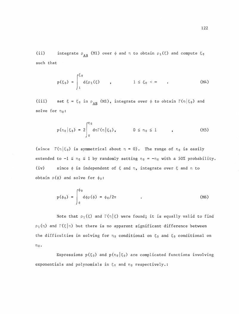
122

(ii) integrate PAB (M1) over ~ and n to obtain Pl(~) and compute ~o

such that

1 ~ ~o < 00 (M4)

(iii) set ~ ~o in PAB (Ml), integrate over ~ to obtain r(nl~o) and

solve for no:

o ~ no ~ 1 (M5)

(since r(nl~o) is symmetrical about n = 0). The range of no is easily

extended to -1 ~ no ~ 1 by randomly setting no = -no with a 50% probability.

(iv) since ¢ 1S independent of ~ and n, integrate over ~ and n to

obtain p(¢) and solve for ¢o:

(M6)

Note that Pl(~) and r(nl~) were found; it is equally valid to find

Pl(n) and r(~ln) but there is no apparent significant difference between

the difficulties in solving for no conditional on ~o and ~o conditional on

no-

Expressions p(~o) and p(nol~o) are complicated functions involving

exponentials and polynomials in ~o and no respectively.:

123

(M7)

and

- exp(-~Rno)[exp(-~R~o)(~2R2(~02 - n0 2) - 2~Rno - 2)]}

(M8)

Random numbers are generated using IMSL [73] subroutine GGUBFS.

The roots of (M7) and (M8) are solved for using IMSL [73] subroutine

&SCNT.

A transformation of variables is used to constrain the ZSCNT

search for no in the range 0 to 1. It was found that at short internuclear

separations, the sine 2 transformation,

y (M9)

where Yt

is the transformed variable, was suitable. At larger distances

(R > 9 au) another transformation,

y exp(y ) (exp(-y ) + exp(y ))-1t . t t

124

had to be employed if ZSCNT were to successfully find no. At large R, the

electron tends to spend a great deal of time close to either nucleus and

so no will be very close to unity, and the sine 2 transformation does not

work well within the ZSCNT algorithm.

The coordinates of all four electrons were chosen independently

using this method.

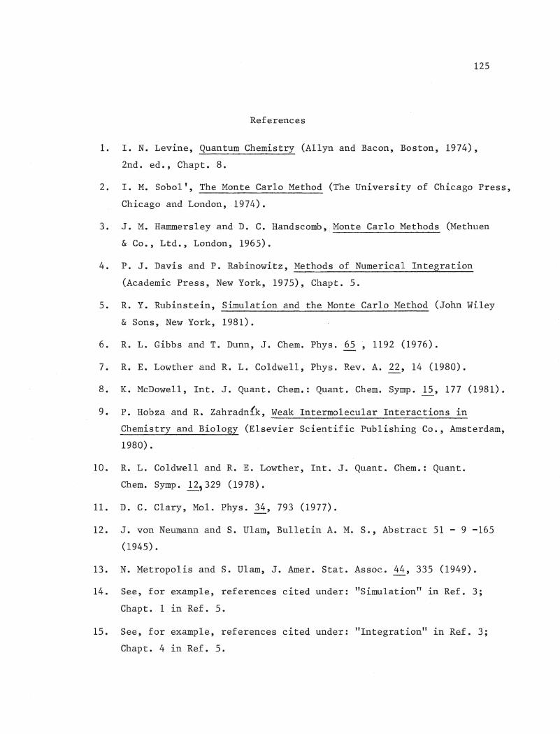
125

References

1. I. N. Levine, Quantum Chemistry (Allyn and Bacon, Boston, 1974),

2nd. ed., Chapt. 8.

2. I. M. Sobol', The Monte Carlo Method (The University of Chicago Press,

Chicago and London, 1974).

3. J. M. Hammersley and D. C. Handscomb, Monte Carlo Methods (Methuen

& Co., Ltd., London, 1965).

4. P. J. Davis and P. Rabinowitz, Methods of Numerical Integration

(Academic Press, New York, 1975), Chapt. 5.

5. R. Y. Rubinstein, Simulation and the Monte Carlo Method (John Wiley

& Sons, New York, 1981).

6. R. L. Gibbs and T. Dunn, J. Chern. Phys. 65 , 1192 (1976).

7. R. E. Lowther and R. L. Coldwell, Phys. Rev. A. 22, 14 (1980).

8. K. McDowell, Int. J. Quant. Chern.: Quant. Chern. Symp. ~' 177 (1981).

9. P. Hobza and R. Zahradn!k, Weak Intermolecular Interactions in

Chemistry and Biology (Elsevier Scientific Publishing Co., Amsterdam,

1980).

10. R. L. Coldwell and R. E. Lowther, Int. J. Quant. Chern.: Quant.

Chern. Symp. g,329 (1978).

11. D. C. Clary, Mol. Phys. 34, 793 (1977).

12. J. von Neumann and S. Ulam, Bulletin A. M. S., Abstract 51 - 9 -165

(1945).

13. N. Metropolis and S. Ulam, J. Amer. Stat. Assoc. 44, 335 (1949).

14. See, for example, references cited under: "Simulation" in Ref. 3;

Chapt. 1 in Ref. 5.

15. See, for example, references cited under: Itlntegration" in Ref. 3;

Chapt. 4 in Ref. 5.

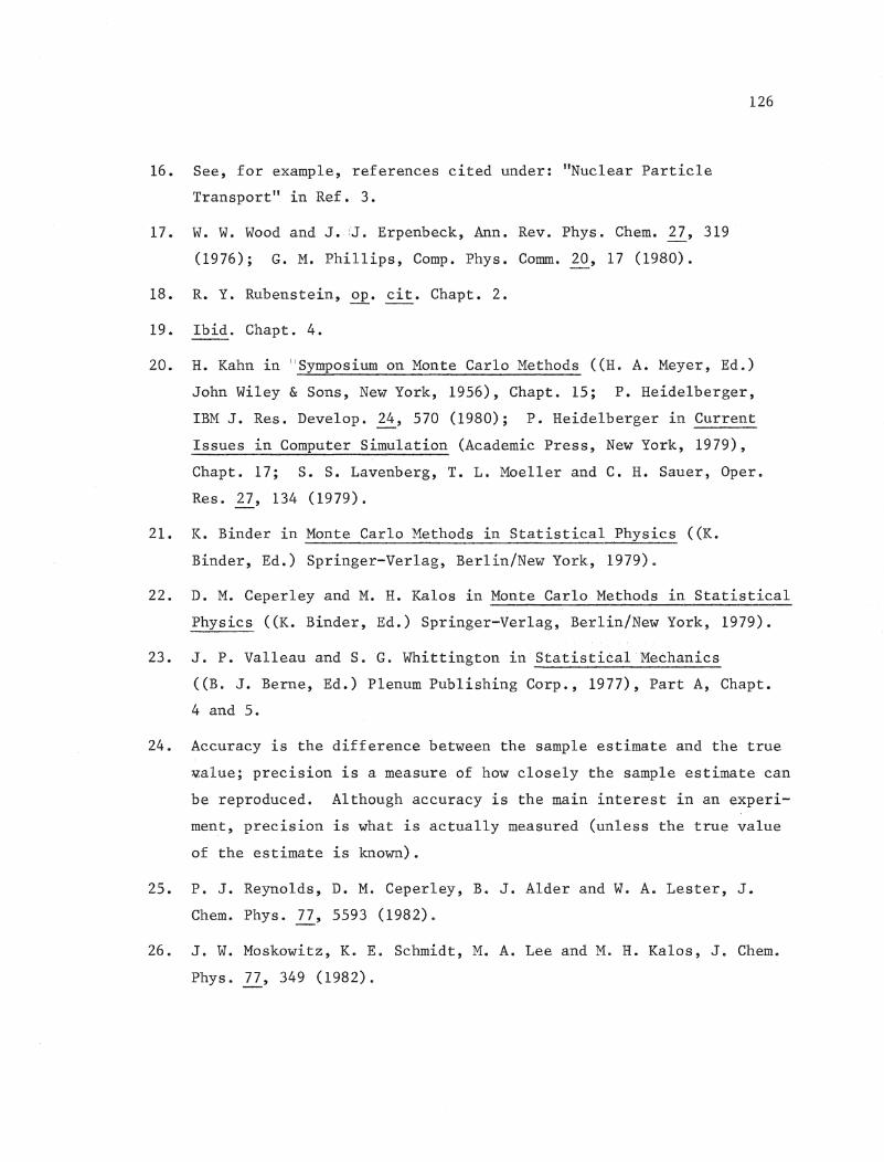
126

16. See, for example, references cited under: "Nuclear Particle

Transport" in Ref. 3.

17. W. W. Wood and J. :'J. Erpenbeck, Ann. Rev. Phys. Chem. '!:2.., 319

(1976); G. M. Phillips, Compo Phys. Comm.20, 17 (1980).

18. R. Y. Rubenstein, Ope cit. Chapt. 2.

19. Ibid. Chapt. 4.

20. H. Kahn in \\Symposium on Monte Carlo Methods «H.A. Meyer, Ed.)

John Wiley & Sons, New York, 1956), Chapt. 15; P. Heidelberger,

IBM J. Res. Develop. 24, 570 (1980); P. Heidelberger in Current

Issues in Computer Simulation (Academic Press, New York, 1979),

Chapt. 17; S. S. Lavenberg, T. L. Moeller and C. H. Sauer, Opere

Res. ~, 134 (1979).

21. K. Binder in Monte Carlo Methods in Statistical Physics «K.

Binder, Ed.) Springer-Verlag, Berlin/New York, 1979).

22. D. M. Ceperley and M. H. Kalas in Monte Carlo Methods in Statistical

Physics «K. Binder, Ed.) Springer-Verlag, Berlin/New York, 1979).

23. J. P. Valleau and S. G. Whittington in Statistical Mechanics

«B. J. Berne, Ed.) Plenum Publishing Corp., 1977), Part A, Chapt.

4 and 5.

24. Accuracy is the difference between the sample estimate and the true

¥alue; precision is a measure of how closely the sample estimate can

be reproduced. Although accuracy is the main interest in an experi­

ment, precision is what is actually measured (unless the true value

of the estimate is known).

25. P. J. Reynolds, D. M. Ceperley, B. J. Alder andW. A. Lester, J.

Chem. Phys. 12, 5593 (1982)$

26. J. W. Moskowitz, K. E. Schmidt, M.A. Lee andM. H. Kalos, J. Chem.

phys.12, 349 (1982).

127

27. J. B. Anderson, J. Chem. Phys. 74, 6307 (1981).

28. C. E. Clark, Opere Res. ~, 603 (1961).

29. R. Y. Rubinstein, Ope cit. Chapt. 3.

30. T. Sasaki, SIAM J. Numer. Anal. ~, 938 (1978).

31. S. M. Rothstein and H. L. Gordon, unpublished work.

32. J. Goodisman and W. Klemperer, J. Chern. Phys. 38, 721 (1963).

33. M. Tin, J. Amer. Stat. Assoc. 60, 294 (1965).

34. H. Cram~r, Mathematical Methods of Statistics (Princeton Univ.

Press, Princeton, 1963), Chapt. 17.

35. W. A. Cochran, Sampling Techniques (Wiley, New York, 1977), 3rd. "

ed., Chapt. 6.

36~ M. H. Hansen, W. N. Hu'rwitz'and W. G. Madow, Sample Survey Methods

and Theory (Wiley, New York, 1953), Vol. I and II, Chapt. 4.

37. H. A. Bethe and E. E. Salpeter, Quantum Mechanics of One- and Two­

Electron Atoms (Springer-Verlag, Berlin, 1957).

38. H. L. Gordon, S. M. Rothstein and T. R•.' Proctor, J. Compo Phys.

!i2, 375 (1982).

39. VA09A, Algorithm 60, Quantum Chemistry Program Exchange, Indiana

University, Bloomington, Indiana 47401.

40. H. Ratajczak and W. J. Orville-Thomas in Molecular Interactions

«H. Ratajczak and W. J. Orville-Thomas, Ed.) John Wiley &Sons,

New York, 1980), Vol. 1, Chapt.l; K. Morokuma and K. Kitaura, loco

cit. Chapt. 2.

41. B. Jeziorski and W. KoKos in Molecular Interactions «H. Ratajczak

and W. J. Orville-Thomas, Ed.) John Wiley & 'Sons, New York, 1982),

Vol. 3, Chapt. 1.

42. t~. Kutzelnigg, Faraday Discuss. Chern. Soc. 62, 185(1977); P.A.

Christiansen, K. S. pitzer et. al., -J. Chem& Phys. 75, 5410 (1981).

128

43. J. S. Winn, J. Chern. Phys. J..!!..., 608 (1981).

44. G. Scoles, Ann. Rev. Phys. Chern. 1l, 81 (1980).

45. A. D. Buckingham in Vibrational Spectroscopy of Molecular Liquids

and Solids «S. Bratos and R. M. Pick, Ed.) NATO Advanced Study

Institute, 1980), Series B 56, pp. 1 - 41.

46. G. G. Maitland, M. Rigby, E. B. Smith and W. A. Wakeham, Inter­

molecular Forces, Their Origin and Determination. (Clarendon Press,

Oxford, 1981).

47. P. Hobza and R. Zahradn{k, Ope cit. Chapt. II.1.b.

48. S. F. Boys and F. Bernardi, Mol. Phys • .!2., 553 (1970).

49. N. S. Ostlund and D. L. Merrifield, Chern. Phys. Lett. 39, 612 (1976).

50. D. R. McLaughlin and H. F. Schaefer III, Chern. Phys. Lett. ~,

244, (1971).

51. P. Bertoncini and A. C. Wahl, J. Chern. Phys. 58, 1259 (1973).

52. B. Liu and A. D. McLean, J. Chern. Phys. 59, 4557 (1973).

53. P. D. Dacre, Phys. Lett. 50, 147 (1977).

54. P. G. Burton, J. Chern. Phys. 3112 (1979).

55. A. L. J. Burgmans, J. M.Farrer and Y. T. Lee, J. Chern. Phys. 64,

1345 (1976).

56. S. M. Blinder, Amer. J. Phys. 33, 431 (1965).

57. G. E. Brown, Many-Body Problems (North-Holland, Amsterdam/London,

1972), pp. 25 - 33.

58. G. Arfkin, Mathematical Methods for Physicists (Academic Press,

New York/London, 1966).

59. The CDC version of HONDO was provided by H. F. King and N. Camp,

Dept. of Chemistry, State University of New York, Buffalo. HONDO

was modified by E. M. Boluk to run on the BURROUGHS 6700. Both

IBM and CDC versions of HONDO are available: Mil Dupuis, J. Rys

129

and H. F. King, HONDO 67, programs 338 and 336, Quantum Chemistry

Program Exchange, University of Indiana, Bloomington, Indiana 47401.

60. C. C. J. Roothan, J. Chern. Phys. J9, 1445 (1951).

61. K. Rudenberg, J. Chern. Phys. 19, 1459 (1951).

62. R. Y. Rubenstein, Ope cit. pp. 124 - 126.

63. R. Jastrow, Phys. Rev. 98, 1479 (1955).

64. N. c. Handy, J. Chern. Phys. ~' 3205 (1969); s. F. Boys and N. C.

Handy, Proc. R. Soc. (London) Series A 309, 209 (1969); 310,. 43

(1969); 310, 63 (1969); 311, 309 (1969).

65. w. Kolos and C. C. J. Roo than , Rev. Mod. Phys. 32, 205 (1960).

66. M. Aubert-Fr~con and C. Le Sech, J. Chern. Phys. 74, 2931 (1981);

J. W. Moskowitz and M. H. Kalas, Int. J. Quant. Chern. 20, 1107 (1981).

67. M. S. Becker, A. A. Broyles and T. Dunn, Phys. Rev. 175, 224 (1968).

68. F. A. Stevens, Jr. and M. A. Pokrant, Phys. Rev. A!, 990 (1973).

69. C. C. Spicer, Appl. Stat. ~' 226 (1972).

70. P. Bertoncini and A. C. Wahl, Phys. Rev. Lett. 25, 991 (1970).

71. D. L. Iglehart and P. A. W. Lewis, "Variance Reduction for Regener­

ative Simulations, I: Internal Control and Stratified Sampling for

Queues," Technical Report No. 86 -.22, Control Analysis Corp., Palo

Alto, Calif. (1976).

72. P. S. Laplace, Theorie Analytique des Probabilit~s~.(Paris, 1920),

3rd. ed.

73. International Mathematical and Statistical Libraries, Inc. IMSL, 1982,

Version 67, Houston, Texas.

74. G. B. Thomas, Jr., Calculus and Analytic Geometry (Addison-Wesley

Publishing Co., Reading, Mass., 1968), 4th. ed., Chapt. 17.6.

75. F. E. Harris and H. H. ~1ichels, Adv. Chem. Phys. ll, 205 (1967).