Quantum Mechanics · Origins of Quantum Mechanics Line spectra of atoms Atomic spectra 4-3 The BohrModel ofthe Hydrogen Atom 163 is the magnitude of E n withn! 1. is called the ground

Quantum Mechanics

Luis A. Anchordoqui

Department of Physics and AstronomyLehman College, City University of New York

Lesson IIIFebruary 19, 2019

L. A. Anchordoqui (CUNY) Quantum Mechanics 2-19-2019 1 / 32

Table of Contents

1 Origins of Quantum MechanicsDimensional analysisLine spectra of atomsBohr’s atomSommerfeld-Wilson quantizationWave-particle dualityHeisenberg’s uncertainty principle


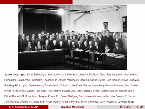
Seated (left to right): Erwin Schrodinger, Irene Joliot-Curie, Niels Bohr, Abram Ioffe, Marie Curie, Paul Langevin, Owen Willans

Richardson, Lord Ernest Rutherford, Theophile de Donder, Maurice de Broglie, Louis de Broglie, Lise Meitner, James Chadwick.

Standing (left to right): Emile Henriot, Francis Perrin, Frederic Joliot-Curie, Werner Heisenberg, Hendrik Kramers, Ernst Stahel,

Enrico Fermi, Ernest Walton, Paul Dirac, Peter Debye, Francis Mott, Blas Cabrera y Felipe, George Gamow, Walther Bothe,

Patrick Blackett, M. Rosenblum, Jacques Errera, Ed. Bauer, Wolfgang Pauli, Jules-mile Verschaffelt, Max Cosyns, E. Herzen,

John Douglas Cockcroft, Charles Ellis, Rudolf Peierls, Auguste Piccard, Ernest Lawrence, Leon Rosenfeld. (October 1933)


Origins of Quantum Mechanics Dimensional analysis

Brice Huang 4 February 22, 2017

4 February 22, 2017

4.1 Dimensional Analysis

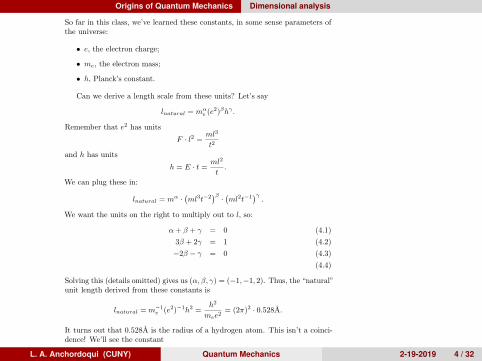
So far in this class, we’ve learned these constants, in some sense parameters ofthe universe:

• e, the electron charge;

• me, the electron mass;

• h, Planck’s constant.

Can we derive a length scale from these units? Let’s say

lnatural = m↵e (e2)�h� .

Remember that e2 has units

F · l2 =ml3

t2

and h has units

h = E · t =ml2

t.

We can plug these in:

lnatural = m↵ ·�ml3t�2

�� ·�ml2t�1

��.

We want the units on the right to multiply out to l, so:

↵+ � + � = 0 (4.1)

3� + 2� = 1 (4.2)

�2� � � = 0 (4.3)

(4.4)

Solving this (details omitted) gives us (↵,�, �) = (�1,�1, 2). Thus, the “natural”unit length derived from these constants is

lnatural = m�1e (e2)�1h2 =

h2

mee2= (2⇡)2 · 0.528A.

It turns out that 0.528A is the radius of a hydrogen atom. This isn’t a coinci-dence! We’ll see the constant

0.528A =

�h2⇡

�2

mee2

again later.

4.2 Matter Waves

De Broglie theorized that all particles have an associated wavelength. A particlewith momentum p has de Broglie wavelength

� =h

p.

23


Origins of Quantum Mechanics Line spectra of atoms

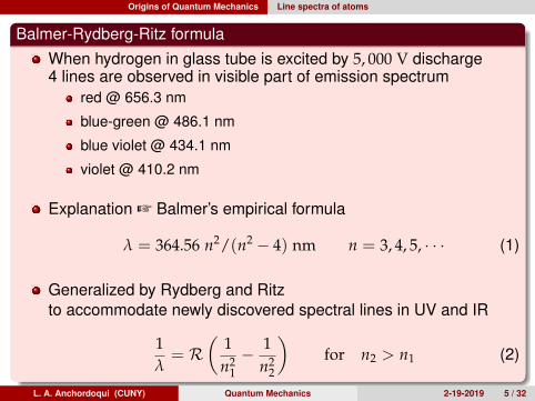
Balmer-Rydberg-Ritz formulaWhen hydrogen in glass tube is excited by 5, 000 V discharge4 lines are observed in visible part of emission spectrum

red @ 656.3 nm

blue-green @ 486.1 nm

blue violet @ 434.1 nm

violet @ 410.2 nm

Explanation + Balmer’s empirical formula

λ = 364.56 n2/(n2 − 4) nm n = 3, 4, 5, · · · (1)

Generalized by Rydberg and Ritzto accommodate newly discovered spectral lines in UV and IR

1λ= R

(1n2

1− 1

n22

)for n2 > n1 (2)



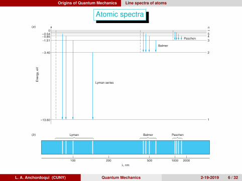
Atomic spectra

4-3 The Bohr Model of the Hydrogen Atom 163

is the magnitude of En with n ! 1. is called the ground state. It is conve-nient to plot these allowed energies of the stationary states as in Figure 4-16. Such aplot is called an energy-level diagram. Various series of transitions between the sta-tionary states are indicated in this diagram by vertical arrows drawn between thelevels. The frequency of light emitted in one of these transitions is the energy differ-ence divided by h according to Bohr’s frequency condition, Equation 4-15. The energyrequired to remove the electron from the atom, 13.6 eV, is called the ionization energy,or binding energy, of the electron.

E1(! "E0)

100 200 500 1000 2000!, nm

(a)

(b)

0–0.54

"5

–0.85 4–1.51 3

–3.40 2

Lyman series

Lyman

Balmer

Paschen

Balmer Paschen

–13.60 1

n

Ene

rgy,

eV

Figure 4-16 Energy-level diagram for hydrogen showing the seven lowest stationary states and the four lowest energytransitions each for the Lyman, Balmer, and Paschen series. There are an infinite number of levels. Their energies are given by

where n is an integer. The dashed line shown for each series is the series limit, corresponding to the energythat would be radiated by an electron at rest far from the nucleus ( ) in a transition to the state with n ! nf for that series.The horizontal spacing between the transitions shown for each series is proportional to the wavelength spacing between the linesof the spectrum. (b) The spectral lines corresponding to the transitions shown for the three series. Notice the regularities withineach series, particularly the short-wavelength limit and the successively smaller separation between adjacent lines as the limit isapproached. The wavelength scale in the diagram is not linear.

nS #En ! "13.6>n2 eV,



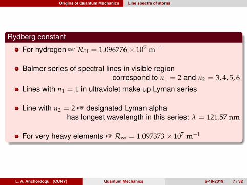
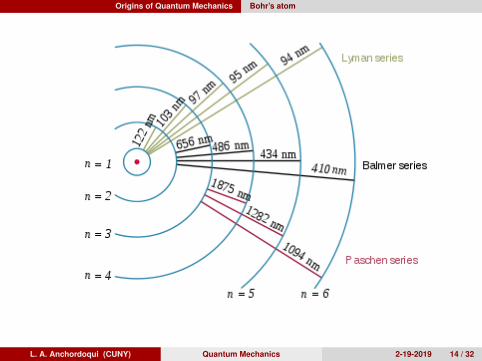
Rydberg constant

For hydrogen + RH = 1.096776× 107 m−1

Balmer series of spectral lines in visible regioncorrespond to n1 = 2 and n2 = 3, 4, 5, 6

Lines with n1 = 1 in ultraviolet make up Lyman series

Line with n2 = 2 + designated Lyman alphahas longest wavelength in this series: λ = 121.57 nm

For very heavy elements + R∞ = 1.097373× 107 m−1



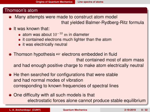
Thomson’s atomMany attempts were made to construct atom model

that yielded Balmer-Rydberg-Ritz formulaIt was known that:

atom was about 10−10 m in diameterit contained electrons much lighter than the atomit was electrically neutral

Thomson hypothesis + electrons embedded in fluidthat contained most of atom mass

and had enough positive charge to make atom electrically neutral

He then searched for configurations that were stableand had normal modes of vibrationcorresponding to known frequencies of spectral lines

One difficulty with all such models is thatelectrostatic forces alone cannot produce stable equilibrium



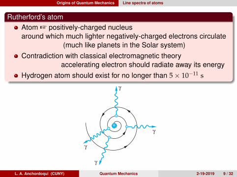
Rutherford’s atomAtom + positively-charged nucleusaround which much lighter negatively-charged electrons circulate

(much like planets in the Solar system)Contradiction with classical electromagnetic theory

accelerating electron should radiate away its energyHydrogen atom should exist for no longer than 5× 10−11 s

The laws of electrodynamics predict that such an accelerating charge will radiatelight of frequency f equal to that of the periodic motion, which in this case is thefrequency of revolution. Thus, classically,

4-13

The total energy of the electron is the sum of the kinetic and the potential energies:

From Equation 4-12, we see that (a result that holds for circular mo-tion in any inverse-square force field), so the total energy can be written as

4-14

Thus, classical physics predicts that, as energy is lost to radiation, theelectron’s orbit will become smaller and smaller while the frequencyof the emitted radiation will become higher and higher, further in-creasing the rate at which energy is lost and ending when the electronreaches the nucleus. (See Figure 4-15a.) The time required for theelectron to spiral into the nucleus can be calculated from classical me-chanics and electrodynamics; it turns out to be less than a microsec-ond. Thus, at first sight, this model predicts that the atom will radiatea continuous spectrum (since the frequency of revolution changescontinuously as the electron spirals in) and will collapse after a veryshort time, a result that fortunately does not occur. Unless excited bysome external means, atoms do not radiate at all, and when excitedatoms do radiate, a line spectrum is emitted, not a continuous one.

Bohr “solved” these formidable difficulties with two decidedlynonclassical postulates. His first postulate was that electrons couldmove in certain orbits without radiating. He called these orbitsstationary states. His second postulate was to assume that the atomradiates when the electron makes a transition from one stationarystate to another (Figure 4-15b) and that the frequency f of the emit-

ted radiation is not the frequency of motion in either stable orbit but is related to theenergies of the orbits by Planck’s theory

4-15

where h is Planck’s constant and Ei and Ef are the energies of the initial and final states.The second assumption, which is equivalent to that of energy conservation with theemission of a photon, is crucial because it deviated from classical theory, which requiresthe frequency of radiation to be that of the motion of the charged particle. Equation 4-15 is referred to as the Bohr frequency condition.

In order to determine the energies of the allowed, nonradiating orbits, Bohr made athird assumption, now known as the correspondence principle, which had profoundimplications:

In the limit of large orbits and large energies, quantum calculations mustagree with classical calculations.

hf ! Ei " Ef

E !kZe2

2r"kZe2

r! "

kZe2

2r! "

1r

12mv2 ! kZe2>2r

E !12mv2 # a"

kZe2

rb

f !v

2$r! akZe2

rmb 1>2 1

2$r! a kZe2

4$2mb 1>2 1r3>2 !

1r3>2

160 Chapter 4 The Nuclear Atom

(a) (b)γ

γ

γ

γ

γ

Figure 4-15 (a) In the classical orbital model,the electron orbits about the nucleus and spiralsinto the center because of the energy radiated.(b) In the Bohr model, the electron orbitswithout radiating until it jumps to anotherallowed radius of lower energy, at which timeradiation is emitted.


Origins of Quantum Mechanics Bohr’s atom

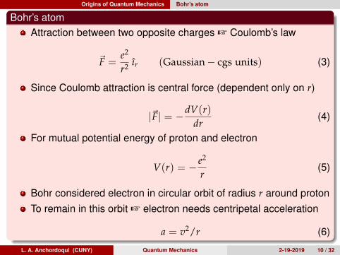
Bohr’s atomAttraction between two opposite charges + Coulomb’s law

~F =e2

r2 ır (Gaussian− cgs units) (3)

Since Coulomb attraction is central force (dependent only on r)

|~F| = −dV(r)dr

(4)

For mutual potential energy of proton and electron

V(r) = − e2

r(5)

Bohr considered electron in circular orbit of radius r around protonTo remain in this orbit + electron needs centripetal acceleration

a = v2/r (6)



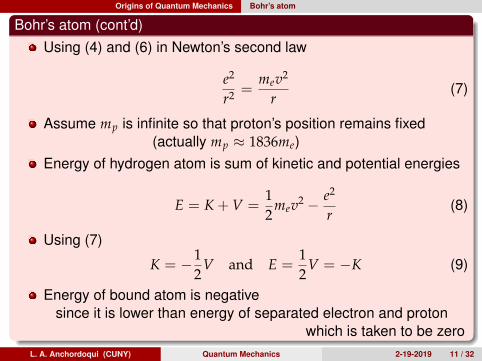
Bohr’s atom (cont’d)Using (4) and (6) in Newton’s second law

e2

r2 =mev2

r(7)

Assume mp is infinite so that proton’s position remains fixed(actually mp ≈ 1836me)

Energy of hydrogen atom is sum of kinetic and potential energies

E = K + V =12

mev2 − e2

r(8)

Using (7)

K = −12

V and E =12

V = −K (9)

Energy of bound atom is negativesince it is lower than energy of separated electron and proton

which is taken to be zeroL. A. Anchordoqui (CUNY) Quantum Mechanics 2-19-2019 11 / 32


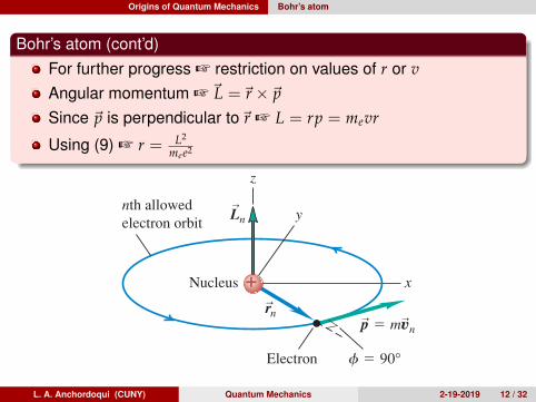
Bohr’s atom (cont’d)For further progress + restriction on values of r or vAngular momentum +~L =~r× ~pSince ~p is perpendicular to~r + L = rp = mevr

Using (9) + r = L2

mee2

39.3 Energy Levels and the Bohr Model of the Atom 1301

the energy levels of a particular atom. Bohr addressed this problem for the caseof the simplest atom, hydrogen, which has just one electron. Let’s look at theideas behind the Bohr model of the hydrogen atom.

Bohr postulated that each energy level of a hydrogen atom corresponds to aspecific stable circular orbit of the electron around the nucleus. In a break withclassical physics, Bohr further postulated that an electron in such an orbit doesnot radiate. Instead, an atom radiates energy only when an electron makes a tran-sition from an orbit of energy Ei to a different orbit with lower energy Ef, emit-ting a photon of energy in the process.

As a result of a rather complicated argument that related the angular frequencyof the light emitted to the angular speed of the electron in highly excited energylevels, Bohr found that the magnitude of the electron’s angular momentum isquantized; that is, this magnitude must be an integral multiple of (Because

the SI units of Planck’s constant h, are the same as the SIunits of angular momentum, usually written as ) Let’s number theorbits by an integer n, where , and call the radius of orbit n andthe speed of the electron in that orbit The value of n for each orbit is called theprincipal quantum number for the orbit. From Section 10.5, Eq. (10.28), themagnitude of the angular momentum of an electron of mass m in such an orbit is

(Fig. 39.21). So Bohr’s argument led to

(39.6)

Instead of going through Bohr’s argument to justify Eq. (39.6), we can use de Broglie’s picture of electron waves. Rather then visualizing the orbiting electronas a particle moving around the nucleus in a circular path, think of it as a sinu-soidal standing wave with wavelength that extends around the circle. A stand-ing wave on a string transmits no energy (see Section 15.7), and electrons inBohr’s orbits radiate no energy. For the wave to “come out even” and join ontoitself smoothly, the circumference of this circle must include some whole numberof wavelengths, as Fig. 39.22 suggests. Hence for an orbit with radius and cir-cumference , we must have where is the wavelength and

According to the de Broglie relationship, Eq. (39.1), the wave-length of a particle with rest mass m moving with nonrelativistic speed is

. Combining and , we find or

This is the same as Bohr’s result, Eq. (39.6). Thus a wave picture of the electronleads naturally to the quantization of the electron’s angular momentum.

Now let’s consider a model of the hydrogen atom that is Newtonian in spiritbut incorporates this quantization assumption (Fig. 39.23). This atom consists ofa single electron with mass m and charge in a circular orbit around a singleproton with charge The proton is nearly 2000 times as massive as the elec-tron, so we can assume that the proton does not move. We learned in Section 5.4that when a particle with mass m moves with speed in a circular orbit withradius its centripetal (inward) acceleration is According to Newton’ssecond law, a radially inward net force with magnitude is needed tocause this acceleration. We discussed in Section 12.4 how the gravitationalattraction provides that inward force for satellite orbits. In hydrogen the force Fis provided by the electrical attraction between the positive proton and the nega-tive electron. From Coulomb’s law, Eq. (21.2),

F = 14pP0

e2

r 2n

F = mv 2n >rn

v 2n >rn.rn,

vn

+e.-e

mvnrn = n h

2p

2prn = nh > mvnln = h > mvn2prn = nlnh > mvn

ln =vn

n = 1, 2, 3, Á .ln2prn = nln,2prn

rn

l

Ln = mvnrn = n h

2p (quantization of angular momentum)

Ln = mvnrn

vn.rnn = 1, 2, 3, Á

kg # m2 > s.

J # s,1 J = 1 kg # m2 > s2,

h > 2p.

hƒ = Ei - Ef

Angular momentum Ln of orbiting electron isperpendicular to plane of orbit (since we takeorigin to be at nucleus) and has magnitudeL 5 mvnrn sin f 5 mvnrn sin 90° 5 mvnrn.

p 5 mvn

f 5 90°

nth allowedelectron orbit

x

z

y

rn

Electron

Nucleus

rr

r

Lnr

r

39.21 Calculating the angular momen-tum of an electron in a circular orbitaround an atomic nucleus.

n ! 2

l

n ! 3

l

n ! 4

l

39.22 These diagrams show the idea offitting a standing electron wave around acircular orbit. For the wave to join ontoitself smoothly, the circumference of theorbit must be an integral number n ofwavelengths.



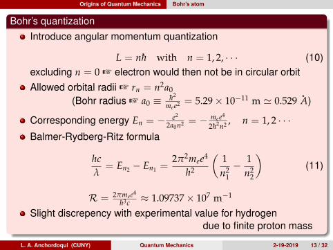
Bohr’s quantizationIntroduce angular momentum quantization

L = nh with n = 1, 2, · · · (10)excluding n = 0 + electron would then not be in circular orbitAllowed orbital radii + rn = n2a0

(Bohr radius + a0 ≡ h2

mee2 = 5.29× 10−11 m ' 0.529 A)

Corresponding energy En = − e2

2a0n2 = − mee4

2h2n2 , n = 1, 2 · · ·Balmer-Rydberg-Ritz formula

hcλ

= En2 − En1 =2π2mee4

h2

(1n2

1− 1

n22

)(11)

R = 2πmee4

h3c ≈ 1.09737× 107 m−1

Slight discrepency with experimental value for hydrogendue to finite proton mass


Origins of Quantum Mechanics Bohr’s atomBrice Huang 4 February 22, 2017

Figure 3: Emission Spectrum of Hydrogen. Image Source: Wikipedia.

4.5 Wilson-Sommerfield Quantization

4.5.1 Quantize All the Things!

So far we’ve discussed two kinds of quantization:

• Quantization of EM energy for a harmonic oscillator into lumps h⌫ led tounderstanding of blackbody radiation;

• Quantization of angular momentum L led to the Bohr atom.

The natural question arising from this is: what else can we quantize?

Wilson and Sommerfield proposed a general rule: if we integrate variableswith respect to their conjugate variables in a closed action, we get a multiple ofh: I

p · dq = nh,

if p, q are conjugate, and the integral is over one cycle.

4.5.2 Case Study: Position and Momentum

Position x and momentum px are conjugate. Consider a harmonic oscillator,oscillating in the x direction. The potential energy of this oscillator V (x) isquadratic in x.

Let’s say the oscillator has energy E and amplitude xmax. Then

E =p2

2m+

1

2kx =

1

2kx2

max.

The oscillator has angular frequency

! =

rk

m,

26



Hydrogen-like ions systems

Generalization for single electron orbiting nucleus

(Z = 1 for hydrogen, Z = 2 for He+, Z = 3 for Li++)

Coulomb potential generalizes to

V(r) = −Ze2

r(12)

Radius of orbit becomes

rn =n2a0

Z(13)

Energy becomes

En = − Z2e2

2a0n2 (14)


Origins of Quantum Mechanics Sommerfeld-Wilson quantization

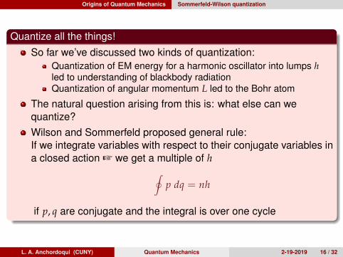
Quantize all the things!

So far we’ve discussed two kinds of quantization:Quantization of EM energy for a harmonic oscillator into lumps hled to understanding of blackbody radiationQuantization of angular momentum L led to the Bohr atom

The natural question arising from this is: what else can wequantize?Wilson and Sommerfeld proposed general rule:If we integrate variables with respect to their conjugate variables ina closed action + we get a multiple of h

∮p dq = nh

if p, q are conjugate and the integral is over one cycle


Origins of Quantum Mechanics Sommerfeld-Wilson quantization

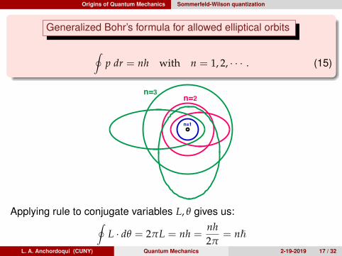
Generalized Bohr’s formula for allowed elliptical orbits

∮p dr = nh with n = 1, 2, · · · . (15)

n=3n=2

n=1

Figure 2. Bohr-Sommerfeld orbitsfor n = 1, 2, 3 (not to scale).

The Bohr model was an important first step in the historical devel-opment of quantum mechanics. It introduced the quantization of atomicenergy levels and gave quantitative agreement with the atomic hydrogenspectrum. With the Sommerfeld-Wilson generalization, it accounted as wellfor the degeneracy of hydrogen energy levels. Although the Bohr model wasable to sidestep the atomic “Hindenberg disaster,” it cannot avoid what wemight call the “Heisenberg disaster.” By this we mean that the assumptionof well-defined electronic orbits around a nucleus is completely contrary tothe basic premises of quantum mechanics. Another flaw in the Bohr pictureis that the angular momenta are all too large by one unit, for example, theground state actually has zero orbital angular momentum (rather than h).

Quantum Mechanics of Hydrogenlike AtomsIn contrast to the particle in a box and the harmonic oscillator, the hydrogenatom is a real physical system that can be treated exactly by quantummechanics. in addition to their inherent significance, these solutions suggestprototypes for atomic orbitals used in approximate treatments of complexatoms and molecules.

For an electron in the field of a nucleus of charge +Ze, the Schrodingerequation can be written

!! h2

2m"2 ! Ze2

r

"!(r) = E !(r) (24)

It is convenient to introduce atomic units in which length is measured in

6

Applying rule to conjugate variables L, θ gives us:∮

L · dθ = 2πL = nh =nh2π

= n}L. A. Anchordoqui (CUNY) Quantum Mechanics 2-19-2019 17 / 32

Origins of Quantum Mechanics Wave-particle duality

de Broglie wavelengthIn view of particle properties for light waves – photons –de Broglie ventured to consider reverse phenomenonAssign wave properties to matter:To every particle with mass m and momentum ~p + associate

λ = h/|~p| (16)

Assignment of energy and momentum to matterin (reversed) analogy to photons

E = hω and |~p| = h|~k| = h/λ (17)



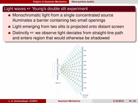
Light waves + Young’s double slit experimentMonochromatic light from a single concentrated sourceilluminates a barrier containing two small openingsLight emerging from two slits is projected onto distant screenDistinctly + we observe light deviates from straight-line pathand enters region that would otherwise be shadowed S E C T I O N 37. 2 • Young’s Double-Slit Experiment 1179

wave to reach point Q . Because the upper wave falls behind the lower one by exactlyone wavelength, they still arrive in phase at Q , and so a second bright fringe appearsat this location. At point R in Figure 37.4c, however, between points P and Q , theupper wave has fallen half a wavelength behind the lower wave. This means thata trough of the lower wave overlaps a crest of the upper wave; this gives rise todestructive interference at point R . For this reason, a dark fringe is observed atthis location.

S1

S2

Barrier

Viewingscreen

max

min

max

min

max

min

max

min

max

(a) (b)

Active Figure 37.2 (a) Schematic diagram of Young’s double-slit experiment. Slits S1and S2 behave as coherent sources of light waves that produce an interference patternon the viewing screen (drawing not to scale). (b) An enlargement of the center of afringe pattern formed on the viewing screen.

At the Active Figures linkat http://www.pse6.com, youcan adjust the slit separationand the wavelength of the lightto see the effect on theinterference pattern.

A

B

Figure 37.3 An interferencepattern involving water waves isproduced by two vibratingsources at the water’s surface. Thepattern is analogous to thatobserved in Young’s double-slitexperiment. Note the regions ofconstructive (A) and destructive(B) interference.

Rich

ard

Meg

na/F

unda

men

tal P

hoto

grap

hs

(a)

Brightfringe Dark

fringe

(b) (c)

Brightfringe

S1

S2

S1

S2

Slits P P P

R

Q

Viewing screen

Q

S2

S1

Figure 37.4 (a) Constructive interference occurs at point P when the waves combine.(b) Constructive interference also occurs at point Q . (c) Destructive interferenceoccurs at R when the two waves combine because the upper wave falls half a wavelengthbehind the lower wave. (All figures not to scale.)

M. C

agne

t, M

. Fra

ncon

, J. C

. Thi

er



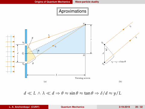
Aproximations

We can describe Young’s experiment quantitatively with the help of Figure 37.5. Theviewing screen is located a perpendicular distance L from the barrier containing two slits,S1 and S2. These slits are separated by a distance d, and the source is monochromatic. Toreach any arbitrary point P in the upper half of the screen, a wave from the lower slit musttravel farther than a wave from the upper slit by a distance d sin !. This distance is calledthe path difference " (lowercase Greek delta). If we assume that r1 and r2 are parallel,which is approximately true if L is much greater than d, then " is given by

" # r 2 $ r1 # d sin! (37.1)

The value of " determines whether the two waves are in phase when they arrive atpoint P. If " is either zero or some integer multiple of the wavelength, then the twowaves are in phase at point P and constructive interference results. Therefore, thecondition for bright fringes, or constructive interference, at point P is

(37.2)

The number m is called the order number. For constructive interference, the ordernumber is the same as the number of wavelengths that represents the path differencebetween the waves from the two slits. The central bright fringe at ! # 0 is called thezeroth-order maximum. The first maximum on either side, where m # %1, is called thefirst-order maximum, and so forth.

When " is an odd multiple of &/2, the two waves arriving at point P are 180° out ofphase and give rise to destructive interference. Therefore, the condition for darkfringes, or destructive interference, at point P is

(37.3)

It is useful to obtain expressions for the positions along the screen of the brightand dark fringes measured vertically from O to P. In addition to our assumption thatL '' d , we assume d '' &. These can be valid assumptions because in practice L isoften on the order of 1 m, d a fraction of a millimeter, and & a fraction of amicrometer for visible light. Under these conditions, ! is small; thus, we can use thesmall angle approximation sin! ! tan!. Then, from triangle OPQ in Figure 37.5a,

d sin!dark # (m ( 12)& (m # 0, %1, %2, ) ) ))

" # d sin! bright # m & (m # 0, %1, %2, ) ) ))

1180 C H A P T E R 37 • Interference of Light Waves

(b)

r2 – r1 = d sin

S1

S2

θd

r1

r2

(a)

d

S1

S2

Q

LViewing screen

θ

θ

P

O

δ

y

r1

r2

θ

Figure 37.5 (a) Geometric construction for describing Young’s double-slit experiment(not to scale). (b) When we assume that r1 is parallel to r2, the path difference betweenthe two rays is r2 $ r1 # d sin !. For this approximation to be valid, it is essential thatL '' d.

Path difference

Conditions for constructiveinterference

Conditions for destructiveinterference

d� L ∧ λ� d⇒ θ ≈ sin θ ≈ tan θ ⇒ δ/d ≈ y/L



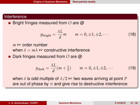
InterferenceBright fringes measured from O are @

ybright =λLd

m m = 0,±1,±2, · · · (18)

m + order numberwhen δ = mλ + constructive interferenceDark fringes measured from O are @

ydark =λLd(m + 1

2 ) m = 0,±1,±2, · · · (19)

when δ is odd multiple of λ/2 + two waves arriving at point Pare out of phase by π and give rise to destructive interference



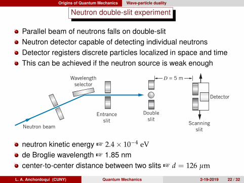
Neutron double-slit experiment

Parallel beam of neutrons falls on double-slitNeutron detector capable of detecting individual neutronsDetector registers discrete particles localized in space and timeThis can be achieved if the neutron source is weak enough

108 Chapter 4 | The Wavelike Properties of Particles

D = 5 m

Entranceslit

Neutron beam

Wavelengthselector

Doubleslit

Scanningslit

Detector

FIGURE 4.11 Double-slit apparatus for neutrons. Thermal neutrons from a reactorare incident on a crystal; scattering through a particular angle selects the energy ofthe neutrons. After passing through the double slit, the neutrons are counted by thescanning slit assembly, which moves laterally.

FIGURE 4.10 Double-slit interfer-ence pattern for electrons.

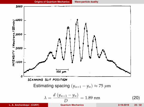
another slit across the beam and measuring the intensity of neutrons passingthrough this “scanning slit.” Figure 4.12 shows the resulting pattern of intensitymaxima and minima, which leaves no doubt that interference is occurring and thatthe neutrons have a corresponding wave nature. The wavelength can be deducedfrom the slit separation using Eq. 3.16 to obtain the spacing between adjacentmaxima, !y = yn+1 − yn. Estimating the spacing !y from Figure 4.12 to be about75 µm, we obtain

λ = d!yD

= (126 µm)(75 µm)5 m

= 1.89 nm

This result agrees very well with the de Broglie wavelength of 1.85 nm selectedfor the neutron beam.

Scanning slit position

100 mm

Inte

nsity

FIGURE 4.12 Intensity pattern ob-served for double-slit interferencewith neutrons. The spacing betweenthe maxima is about 75 µm. [Source:R. Gahler and A. Zeilinger, AmericanJournal of Physics 59, 316 (1991).]

It is also possible to do a similar experiment with atoms. In this case, asource of helium atoms formed a beam (of velocity corresponding to a kineticenergy of 0.020 eV) that passed through a double slit of separation 8 µm andwidth 1 µm. Again a scanning slit was used to measure the intensity of the beampassing through the double slit. Figure 4.13 shows the resulting intensity pattern.Although the results are not as dramatic as those for electrons and neutrons, thereis clear evidence of interference maxima and minima, and the separation of themaxima gives a wavelength that is consistent with the de Broglie wavelength (seeProblem 8).

10 mm


Inte

nsity

FIGURE 4.13 Intensity pattern ob-served for double-slit interferencewith helium atoms. [Source: O. Car-nal and J. Mlynek, Physical ReviewLetters 66, 2689 (1991).]

Diffraction can be observed with even larger objects. Figure 4.14 shows thepattern produced by fullerene molecules (C60) in passing through a diffractiongrating with a spacing of d = 100 nm. The diffraction pattern was observed ata distance of 1.2 m from the grating. Estimating the separation of the maximain Figure 4.14 as 50 µm, we get the angular separation of the maxima to beθ ≈ tan θ = (50 µm)/(1.2 m) = 4.2 × 10−5 rad, and thus λ = d sin θ = 4.2 pm.For C60 molecules with a speed of 117 m/s used in this experiment, the expectedde Broglie wavelength is 4.7 pm, in good agreement with our estimate from thediffraction pattern.

In this chapter we have discussed several interference and diffractionexperiments using different particles—electrons, protons, neutrons, atoms,and molecules. These experiments are not restricted to any particular type ofparticle or to any particular type of observation. They are examples of a generalphenomenon, the wave nature of particles, that was unobserved before 1920because the necessary experiments had not yet been done. Today this wavenature is used as a basic tool by scientists. For example, neutron diffraction

neutron kinetic energy + 2.4× 10−4 eVde Broglie wavelength + 1.85 nmcenter-to-center distance between two slits + d = 126 µm



This article is copyrighted as indicated in the article. Reuse of AAPT content is subject to the terms at: http://scitation.aip.org/termsconditions. Downloaded to IP:216.165.95.75 On: Fri, 16 Oct 2015 15:50:23

Estimating spacing (yn+1 − yn) ≈ 75 µm

λ =d (yn+1 − yn)

D= 1.89 nm (20)


Origins of Quantum Mechanics Heisenberg’s uncertainty principle

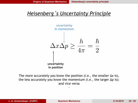
Heisenberg’s Uncertainty Principle

The more accurately you know the position (i.e., the smaller Δx is), the less accurately you know the momentum (i.e., the larger Δp is);

and vice versa

uncertaintyin momentum

uncertaintyin position

5



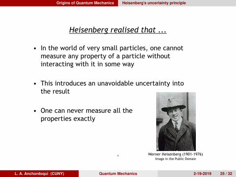
Heisenberg realised that ...

• In the world of very small particles, one cannot measure any property of a particle without interacting with it in some way

• This introduces an unavoidable uncertainty into the result

• One can never measure all the properties exactly

Werner Heisenberg (1901-1976)Image in the Public Domain

6



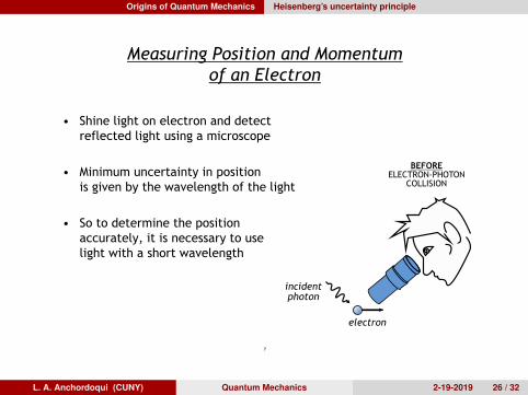
Measuring Position and Momentum of an Electron

• Shine light on electron and detectreflected light using a microscope

• Minimum uncertainty in position is given by the wavelength of the light

• So to determine the position accurately, it is necessary to use light with a short wavelength

BEFORE ELECTRON-PHOTON

COLLISION

incidentphoton

electron

7



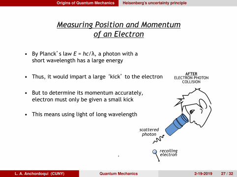
Measuring Position and Momentum

• By Planc ’k s law E = hc/λ, a photon with a short wavelength has a large energy

• Thus, it would impart a large ‘kick’ to the electron

• But to determine its momentum accurately, electron must only be given a small kick

• This means using light of long wavelength

of an Electron

AFTERELECTRON-PHOTON

COLLISION

scatteredphoton

recoilingelectron8



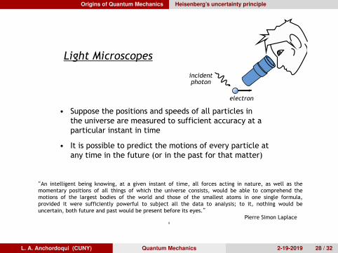
Light Microscopes

• Suppose the positions and speeds of all particles in the universe are measured to sufficient accuracy at a particular instant in time

• It is possible to predict the motions of every particle at any time in the future (or in the past for that matter)

“An intelligent being knowing, at a given instant of time, all forces acting in nature, as well as themomentary positions of all things of which the universe consists, would be able to comprehend themotions of the largest bodies of the world and those of the smallest atoms in one single formula,provided it were sufficiently powerful to subject all the data to analysis; to it, nothing would beuncertain, both future and past would be present before its eyes.”

Pierre Simon Laplace

incidentphoton

electron

9



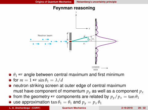
Feynman reasoning

the fact that the photomultiplier detects faint light as a sequence of individual“spots” can’t be explained in wave terms.

Probability and UncertaintyAlthough photons have energy and momentum, they are nonetheless very differ-ent from the particle model we used for Newtonian mechanics in Chapters 4through 8. The Newtonian particle model treats an object as a point mass. We candescribe the location and state of motion of such a particle at any instant withthree spatial coordinates and three components of momentum, and we can thenpredict the particle’s future motion. This model doesn’t work at all for photons,however: We cannot treat a photon as a point object. This is because there arefundamental limitations on the precision with which we can simultaneouslydetermine the position and momentum of a photon. Many aspects of a photon’sbehavior can be stated only in terms of probabilities. (In Chapter 39 we will findthat the non-Newtonian ideas we develop for photons in this section also apply toparticles such as electrons.)

To get more insight into the problem of measuring a photon’s position andmomentum simultaneously, let’s look again at the single-slit diffraction of light(Fig. 38.17). Suppose the wavelength is much less than the slit width a. Thenmost (85%) of the photons go into the central maximum of the diffraction pat-tern, and the remainder go into other parts of the pattern. We use to denote theangle between the central maximum and the first minimum. Using Eq. (36.2)with we find that is given by Since we assume itfollows that is very small, is very nearly equal to (in radians), and

(38.12)

Even though the photons all have the same initial state of motion, they don’t allfollow the same path. We can’t predict the exact trajectory of any individual pho-ton from knowledge of its initial state; we can only describe the probability thatan individual photon will strike a given spot on the screen. This fundamentalindeterminacy has no counterpart in Newtonian mechanics.

Furthermore, there are fundamental uncertainties in both the position and themomentum of an individual particle, and these uncertainties are related insepara-bly. To clarify this point, let’s go back to Fig. 38.17. A photon that strikes thescreen at the outer edge of the central maximum, at angle must have a compo-nent of momentum in the y-direction, as well as a component in the x-direction,despite the fact that initially the beam was directed along the x-axis. From thegeometry of the situation the two components are related by Since is small, we may use the approximation andtan u1 = u1,u1

py>px = tan u1.

pxpy

u1,

u1 = la

u1sin u1u1

l = a,sin u1 = l>a.u1m = 1,

u1

l

1274 CHAPTER 38 Photons: Light Waves Behaving as Particles

38.17 Interpreting single-slit diffractionin terms of photon momentum. px and py are the momentum components

for a photon striking the outer edge ofthe central maximum, at angle u1.

py

px

Screen

a

Slit

Photons of monochromatic light

Diffractionpattern

u1

pS

PhET: Fourier: Making WavesPhET: Quantum Wave InterferenceActivPhysics 17.6: Uncertainty Principle

Feynman9 was that both electrons and photons behave in their own inimitableway. This is like nothing we have seen before, because we do not live at the verytiny scale of atoms, electrons, and photons.

Perhaps the best way to crystallize our ideas about the wave – particle du-ality is to consider a “simple” double-slit electron diffraction experiment.This experiment highlights much of the mystery of the wave – particle para-dox, shows the impossibility of measuring simultaneously both wave and par-ticle properties, and illustrates the use of the wavefunction, !, in determin-ing interference effects. A schematic of the experiment with monoenergetic(single-wavelength) electrons is shown in Figure 5.28. A parallel beam ofelectrons falls on a double slit, which has individual openings much smallerthan D so that single-slit diffraction effects are negligible. At a distance fromthe slits much greater than D is an electron detector capable of detectingindividual electrons. It is important to note that the detector always regis-ters discrete particles localized in space and time. In a real experiment thiscan be achieved if the electron source is weak enough (see Fig. 5.29): In allcases if the detector collects electrons at different positions for a longenough time, a typical wave interference pattern for the counts perminute or probability of arrival of electrons is found (see Fig. 5.28). Ifone imagines a single electron to produce in-phase “wavelets” at the slits,standard wave theory can be used to find the angular separation, ", of the

180 CHAPTER 5 MATTER WAVES

9R. Feynman, The Character of Physical Law, Cambridge, MA, MIT Press, 1982.

D

A

B

θ

Electrons

θ

x

y

Electrondetector

countsmin

Figure 5.28 Electron diffraction. D is much greater than the individual slit widthsand much less than the distance between the slits and the detector.

Copyright 2005 Thomson Learning, Inc. All Rights Reserved.

Feynman9 was that both electrons and photons behave in their own inimitableway. This is like nothing we have seen before, because we do not live at the verytiny scale of atoms, electrons, and photons.

Perhaps the best way to crystallize our ideas about the wave – particle du-ality is to consider a “simple” double-slit electron diffraction experiment.This experiment highlights much of the mystery of the wave – particle para-dox, shows the impossibility of measuring simultaneously both wave and par-ticle properties, and illustrates the use of the wavefunction, !, in determin-ing interference effects. A schematic of the experiment with monoenergetic(single-wavelength) electrons is shown in Figure 5.28. A parallel beam ofelectrons falls on a double slit, which has individual openings much smallerthan D so that single-slit diffraction effects are negligible. At a distance fromthe slits much greater than D is an electron detector capable of detectingindividual electrons. It is important to note that the detector always regis-ters discrete particles localized in space and time. In a real experiment thiscan be achieved if the electron source is weak enough (see Fig. 5.29): In allcases if the detector collects electrons at different positions for a longenough time, a typical wave interference pattern for the counts perminute or probability of arrival of electrons is found (see Fig. 5.28). Ifone imagines a single electron to produce in-phase “wavelets” at the slits,standard wave theory can be used to find the angular separation, ", of the

180 CHAPTER 5 MATTER WAVES

9R. Feynman, The Character of Physical Law, Cambridge, MA, MIT Press, 1982.

D

A

B

θ

Electrons

θ

x

y

Electrondetector

countsmin

Figure 5.28 Electron diffraction. D is much greater than the individual slit widthsand much less than the distance between the slits and the detector.

Copyright 2005 Thomson Learning, Inc. All Rights Reserved.

108 Chapter 4 | The Wavelike Properties of Particles

D = 5 m

Entranceslit

Neutron beam

Wavelengthselector

Doubleslit

Scanningslit

Detector

FIGURE 4.11 Double-slit apparatus for neutrons. Thermal neutrons from a reactorare incident on a crystal; scattering through a particular angle selects the energy ofthe neutrons. After passing through the double slit, the neutrons are counted by thescanning slit assembly, which moves laterally.

FIGURE 4.10 Double-slit interfer-ence pattern for electrons.

another slit across the beam and measuring the intensity of neutrons passingthrough this “scanning slit.” Figure 4.12 shows the resulting pattern of intensitymaxima and minima, which leaves no doubt that interference is occurring and thatthe neutrons have a corresponding wave nature. The wavelength can be deducedfrom the slit separation using Eq. 3.16 to obtain the spacing between adjacentmaxima, !y = yn+1 − yn. Estimating the spacing !y from Figure 4.12 to be about75 µm, we obtain

λ = d!yD

= (126 µm)(75 µm)5 m

= 1.89 nm

This result agrees very well with the de Broglie wavelength of 1.85 nm selectedfor the neutron beam.


100 mm

Inte

nsity

FIGURE 4.12 Intensity pattern ob-served for double-slit interferencewith neutrons. The spacing betweenthe maxima is about 75 µm. [Source:R. Gahler and A. Zeilinger, AmericanJournal of Physics 59, 316 (1991).]

It is also possible to do a similar experiment with atoms. In this case, asource of helium atoms formed a beam (of velocity corresponding to a kineticenergy of 0.020 eV) that passed through a double slit of separation 8 µm andwidth 1 µm. Again a scanning slit was used to measure the intensity of the beampassing through the double slit. Figure 4.13 shows the resulting intensity pattern.Although the results are not as dramatic as those for electrons and neutrons, thereis clear evidence of interference maxima and minima, and the separation of themaxima gives a wavelength that is consistent with the de Broglie wavelength (seeProblem 8).

10 mm


Inte

nsity

FIGURE 4.13 Intensity pattern ob-served for double-slit interferencewith helium atoms. [Source: O. Car-nal and J. Mlynek, Physical ReviewLetters 66, 2689 (1991).]

Diffraction can be observed with even larger objects. Figure 4.14 shows thepattern produced by fullerene molecules (C60) in passing through a diffractiongrating with a spacing of d = 100 nm. The diffraction pattern was observed ata distance of 1.2 m from the grating. Estimating the separation of the maximain Figure 4.14 as 50 µm, we get the angular separation of the maxima to beθ ≈ tan θ = (50 µm)/(1.2 m) = 4.2 × 10−5 rad, and thus λ = d sin θ = 4.2 pm.For C60 molecules with a speed of 117 m/s used in this experiment, the expectedde Broglie wavelength is 4.7 pm, in good agreement with our estimate from thediffraction pattern.

In this chapter we have discussed several interference and diffractionexperiments using different particles—electrons, protons, neutrons, atoms,and molecules. These experiments are not restricted to any particular type ofparticle or to any particular type of observation. They are examples of a generalphenomenon, the wave nature of particles, that was unobserved before 1920because the necessary experiments had not yet been done. Today this wavenature is used as a basic tool by scientists. For example, neutron diffraction

We can describe Young’s experiment quantitatively with the help of Figure 37.5. Theviewing screen is located a perpendicular distance L from the barrier containing two slits,S1 and S2. These slits are separated by a distance d, and the source is monochromatic. Toreach any arbitrary point P in the upper half of the screen, a wave from the lower slit musttravel farther than a wave from the upper slit by a distance d sin !. This distance is calledthe path difference " (lowercase Greek delta). If we assume that r1 and r2 are parallel,which is approximately true if L is much greater than d, then " is given by

" # r 2 $ r1 # d sin! (37.1)

The value of " determines whether the two waves are in phase when they arrive atpoint P. If " is either zero or some integer multiple of the wavelength, then the twowaves are in phase at point P and constructive interference results. Therefore, thecondition for bright fringes, or constructive interference, at point P is

(37.2)

The number m is called the order number. For constructive interference, the ordernumber is the same as the number of wavelengths that represents the path differencebetween the waves from the two slits. The central bright fringe at ! # 0 is called thezeroth-order maximum. The first maximum on either side, where m # %1, is called thefirst-order maximum, and so forth.

When " is an odd multiple of &/2, the two waves arriving at point P are 180° out ofphase and give rise to destructive interference. Therefore, the condition for darkfringes, or destructive interference, at point P is

(37.3)

It is useful to obtain expressions for the positions along the screen of the brightand dark fringes measured vertically from O to P. In addition to our assumption thatL '' d , we assume d '' &. These can be valid assumptions because in practice L isoften on the order of 1 m, d a fraction of a millimeter, and & a fraction of amicrometer for visible light. Under these conditions, ! is small; thus, we can use thesmall angle approximation sin! ! tan!. Then, from triangle OPQ in Figure 37.5a,

d sin!dark # (m ( 12)& (m # 0, %1, %2, ) ) ))

" # d sin! bright # m & (m # 0, %1, %2, ) ) ))

1180 C H A P T E R 37 • Interference of Light Waves

(b)

r2 – r1 = d sin

S1

S2

θd

r1

r2

(a)

d

S1

S2

Q

LViewing screen

θ

θ

P

O

δ

y

r1

r2

θ

Figure 37.5 (a) Geometric construction for describing Young’s double-slit experiment(not to scale). (b) When we assume that r1 is parallel to r2, the path difference betweenthe two rays is r2 $ r1 # d sin !. For this approximation to be valid, it is essential thatL '' d.

Path difference

Conditions for constructiveinterference

Conditions for destructiveinterference

θ1 + angle between central maximum and first minimumfor m = 1 + sin θ1 = λ/dneutron striking screen at outer edge of central maximummust have component of momentum py as well as a component pxfrom the geometry + components are related by py/px = tan θ1use approximation tan θ1 = θ1 and py = px θ1



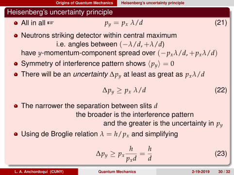
Heisenberg’s uncertainty principleAll in all + py = px λ/d (21)

Neutrons striking detector within central maximumi.e. angles between (−λ/d,+λ/d)

have y-momentum-component spread over (−pxλ/d,+pxλ/d)Symmetry of interference pattern shows 〈py〉 = 0There will be an uncertainty ∆py at least as great as pxλ/d

∆py ≥ px λ/d (22)

The narrower the separation between slits dthe broader is the interference pattern

and the greater is the uncertainty in py

Using de Broglie relation λ = h/px and simplifying

∆py ≥ pxh

pxd=

hd

(23)



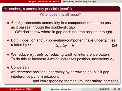
Heisenberg’s uncertainty principle (cont’d)What does this all mean?

d ≡ ∆y represents uncertainty in y-component of neutron positionas it passes through the double-slit gap

(We don’t know where in gap each neutron passes through)

Both y-position and y-momentum-component have uncertaintiesrelated by + ∆py ∆y ≥ h (24)

We reduce ∆py only by reducing width of interference patternTo do this + increase d which increases position uncertainty ∆y

Converselywe decrease position uncertainty by narrowing doubl-slit gapinterference pattern broadens

and corresponding momentum uncertainty increases



Bibliography

1 David J. Griffiths; ISBN: 0-13-124405-12 Eugen Merzbacher; ISBN: 0-471-88702-13 Steven Weinberg; ISBN: 978-11071116604 Claude Cohen-Tannoudji, Bernard Diu, Franck Laloe;

ISBN: 978-0471164333


Documents

Quantum Mechanics · Origins of Quantum Mechanics Line spectra of atoms Atomic spectra 4-3 The BohrModel ofthe Hydrogen Atom 163 is the magnitude of E n withn! 1. is called the ground