Embed Size (px)
Citation preview
IL NUOVO CIMENTO Vol. ?, N. ? ?
Quantum mechanics, matter waves, and moving clocks
Holger Muller(1)
(1) Department of Physics, 366 Le Conte Hall, University of California, Berkeley, CA 94720,USA
Summary. — This paper is divided into three parts. In the first (section 1), wedemonstrate that all of quantum mechanics can be derived from the fundamentalproperty that the propagation of a matter wave packet is described by the samegravitational and kinematic time dilation that applies to a clock. We will do so inseveral steps, first deriving the Schrodinger equation for a nonrelativistic particlewithout spin in a weak gravitational potential, and eventually the Dirac equation incurved space-time describing the propagation of a relativistic particle with spin instrong gravity.In the second part (sections 2-4), we present interesting consequences of the abovequantum mechanics: that it is possible to use wave packets as a reference for aclock, to test general relativity, and to realize a mass standard based on a pro-posed redefinition of the international system of units, wherein the Planck con-stant would be assigned a fixed value. The clock achieved an absolute accuracyof 4 parts per billion (ppb). The experiment yields the fine structure constantα = 7.297 352 589(15)× 10−3 with 2.0 ppb accuracy. We present improvements thathave reduced the leading systematic error about 8-fold and improved the statisticaluncertainty to 0.33 ppb in 6 hours of integration time, referred to α.In the third part (sections 5-7), we present possible future experiments with atominterferometry: A gravitational Aharonov-Bohm experiment and its application asa measurement of Newton’s gravitational constant, antimatter interferometry, inter-ferometry with charged particles, and interferometry in space.We will give a review of previously published material when appropriate, but willfocus on new aspects that haven’t been published before.
PACS 03.75.Dg –PACS . – 37.25.+k.PACS 03.65.Pm –PACS . – 04.62.+v.PACS 31.15.xk –PACS . – 03.65.Ta.
c© Societa Italiana di Fisica 1
arX
iv:1
312.
6449
v1 [
quan
t-ph
] 2
3 D
ec 2
013
2 HOLGER MULLER
4 1. Quantum mechanics as a theory of waves oscillating at the Compton frequency5 1
.1. Notation
5 1.2. De Broglie’s relations
6 1.3. Construction of a path integral
8 1.4. Derivation of the Schrodinger equation
9 1.5. Derivation of the Dirac equation without gravity
10 1.5.1. Re-writing the proper time
10 1.5.2. Derivation of the Dirac equation
11 1.5.3. Interpretation
12 1.5.4. Derivation of the matter-waves-as-clocks picture from the Dirac
equation12 1
.6. Derivation of a Dirac equation with electromagnetic potentials
13 1.7. Derivation of the Dirac equation with gravity, in curved space-time
13 1.7.1. Derivation
16 1.7.2. A simple limiting case
16 1.7.3. Comparison to the usual form
18 1.8. Discussion
18 1.9. Review of some counterarguments
18 1.10. Conclusion
19 2. Brief summary of basics of atom interferometers20 2
.1. Mach-Zehnder atom interferometers as redshift measurements
20 2.1.1. Conventional redshift measurements with clocks
20 2.1.2. Correcting for time dilation
21 2.1.3. Experiment with piecewise freely falling clocks
21 2.1.4. Comparison to atom interferometer
22 2.1.5. Examples where interpretations as force measurements fail
23 3. Tests of relativity24 3
.1. The standard model extension
25 3.1.1. The Fermionic sector
25 3.1.2. The gravitational sector
26 3.1.3. Electromagnetic sector
27 3.2. Test of gravity’s isotropy
27 3.2.1. Hypothetical signal
27 3.2.2. Data analysis and results
28 3.3. Test of the Equivalence principle
30 3.3.1. Gravity Probe A
30 3.3.2. Null Redshift Tests
31 3.3.3. Nuclear Transitions
31 3.3.4. Matter-wave tests
31 3.3.5. Conclusion
31 3.3.6. Influence of nuclear structure
33 3.4. Global limits
34 4. Time, mass, and the fine structure constant35 4
.1. Our atomic-fountain interferometer
35 4.1.1. Bragg diffraction
35 4.2. Simultaneous interferometers
35 4.2.1. Laser system
37 4.2.2. Coriolis compensation
37 4.3. The Compton clock: nonrelativistic treatment.
37 4.4. Relativistic treatment
38 4.4.1. Free evolution phase
38 4.4.2. Laser phase
39 4.5. Experiment
41 4.5.1. Is there a “clock ticking at the Compton frequency”?
QUANTUM MECHANICS, MATTER WAVES, AND MOVING CLOCKS 3
43 4.6. The fine structure constant
43 4.7. Further improvements
44 4.8. Atom interferometry and the SI: Mass standards
45 5. Atom interferometer in a cavity45 5
.1. Gravitational Aharonov-Bohm effect
45 5.1.1. The Aharonov-Bohm (AB) effect
46 5.1.2. Gravitational Aharonov-Bohm effect
47 5.1.3. Signal size
47 5.1.4. Relation to other proposed gravitational AB effects
47 5.2. Newton’s gravitational constant G
49 5.3. Experimental setup
50 5.4. Systematic effects
51 5.4.1. Zeeman effect
51 5.4.2. Lattice potential/AC Stark effect
52 5.4.3. Vibrations
53 5.4.4. Mean field shift
53 5.4.5. Test masses and atom positions
53 5.4.6. Rotations
54 5.4.7. Source masses
54 5.5. Matter waves and the measurement of proper time
54 6. Antimatter interferometry55 6
.1. The equivalence principle for antimatter
55 6.1.1. Energy conservation
55 6.1.2. Supernova 1987A
55 6.1.3. Virtual antiparticles
55 6.1.4. The Kaon system / electrons and positrons in Penning traps
56 6.1.5. Bound kinetic energy
56 6.2. Previous experiments with charged particles
56 6.3. Setup
58 6.4. Interferometry with charged particles
60 6.4.1. Testing the equivalence principle for charged particles
60 6.4.2. Phase calculation for a single interferometer
60 6.4.3. Nonzero initial position and velocity
61 6.4.4. Double diffraction
61 6.4.5. Trap anharmonicity
62 6.4.6. Non-closure of the interferometer
63 6.4.7. Decoherence from axial damping
63 6.4.8. Example
63 7. Interferometry in space63 7
.1. Concept
64 7.2. Test of the equivalence principle
65 7.2.1. Advantages of quantum tests of the EEP in space
65 7.3. Recoil measurements and mass standard
65 7.3.1. Fine structure constant
66 7.3.2. Absolute masses
66 7.4. Design parameters
68 7.5. Inversion of the setup
68 8. Summary and outlook69 References
4 HOLGER MULLER
1. – Quantum mechanics as a theory of waves oscillating at the Comptonfrequency
We will show that all of quantum mechanics can be derived from a picture of matterwaves as clocks together with simple assumptions such as the principle of superposition.This picture assumes that a quantum mechanical wave packet has an oscillation frequencyof ωC = mc2/~, where m is the particle’s mass, c the velocity of light, and ~ the reducedPlanck constant. The oscillation frequency is shifted by the gravitational redshift andtime dilation as the particle moves through space and time. The propagation of arbitaryquantum states can be decomposed into such wave-packets (“matter-wave clocks”) takingall possible paths through phase-space. We will show that this path integral formalismwill yield the quantum mechanical wave equations, starting with the Schrodinger equationfor nonrelativistic, spinless particles, then for relativistic particles with spin, first withoutgravity, then in curved space-time. This shows that the picture of matter wave packetsas Compton frequency clocks is not just exact. It can even be used to re-derive all ofquantum mechanics.
The description of matter waves as matter-wave clocks has been the basis of deBroglie’s invention of matter waves [1]. It has recently been applied to tests of generalrelativity [2, 3, 4, 5, 6, 7, 8, 9, 10, 11, 12], matter-wave experiments [13, 14, 15, 16, 17, 18,19, 20, 21, 22], the foundations of quantum mechanics [23, 24], quantum space-time deco-herence [25], the matter wave clock/mass standard [26, 29, 30], and led to a discussion onthe role of the proper time in quantum mechanics [31, 32]. It is generally covariant andthus well-suited for use in curved space-time, e.g., gravitational waves [33, 34, 35, 36].It has also given rise to a fair amount of controversy [37, 38, 39, 40, 41, 42, 43, 44, 45].Within the broader context of quantum mechanics, however, this description has beenabandoned, in part because it could not be used to derive a relativistic quantum theory,or explain spin.
The descriptions that replaced the clock picture achieve these goals, but do not mo-tivate the concepts used. For example, the Dirac equation can be derived from a La-grangian density, where ψ takes the role of the coordinates: LD = i~cψγµ∂µψ−mc2ψψ,where the γµ are the Dirac matrices, the operator ψ annihilates, and ψ creates, a par-ticle, and ∂µ ≡ ∂/∂xµ. This Lagrangian density is quadratic in ψ and thereby allowsto construct a path integral in Hilbert space. It, however, takes the existence of spinorsand Dirac matrices for granted rather than explaining or motivating the need for them.
We shall construct a path integral directly from a Lagrangian that is a function of thespace-time coordinates L = −mc2dτ/dt, where t is the coordinate time, without makinga nonrelativistic approximation or introducing additional fields. This will require us tointroduce the Dirac matrices and spinors, and will thus explain their use. Since the phaseaccumulated by a wave packet is given by φ = −L/~, it corresponds to a description ofmatter waves as clocks. We will thus arrive at a space-time path integral [46] in whichφ = −ωCτ is maintained exactly, that is equivalent to the Dirac equation.
This derivation shows that De Broglie’s matter wave theory naturally leads to particleswith spin-1/2. It relates to Feynman’s search for a formula for the amplitude of a pathin 3+1 space and time dimensions which is equivalent to the Dirac equation [47, 48]. Ityields a new intuitive interpretation of the propagation of a Dirac particle and reproducesall results of standard quantum mechanics, including those supposedly at odds with it.Thus, it illuminates the role of the gravitational redshift and the proper time in quantummechanics. Finally, we hope it offers an intuitive way to think about quantum mechanicsand its possible generalizations.
QUANTUM MECHANICS, MATTER WAVES, AND MOVING CLOCKS 5
1.1. Notation. – We use letters from the second half of the Greek alphabet κ, λ, µ, ν, . . . =
0, 1, 2, 3 to denote the space-time coordinates. Letters from the second half of the Latinalphabet j, k, l,m . . . denote the spatial coordinates. In curved space-time, we shallemploy both a coordinate frame with a metric gµν and a local Lorentz frame with aMinkowski metric ηαβ . The determinant of gµν is denoted g. Greek letters from thestart of the alphabet α, β, . . . will denote coordinates in the local Lorentz frame, the let-ters a, b, c, . . . denote the spatial coordinates in the local Lorentz frame. The two framesare connected by the vierbein gµν = eµαe
νβη
αβ . Our Minkowski metric has a signature
−+ ++. The conventional Dirac matrices in the coordinate frame are αk and β as wellas γ0 = β, γk = γ0αk and σαβ = 1
2 [γα, γβ ], where [a, b] = ab− ba is the commutator. Inweak gravitational fields, we write the metric as gµν = ηµν + hµν , where |hµν | 1.
1.2. De Broglie’s relations. – De Broglie started with Einstein’s equation E = mc2 and
Planck’s E = hν, where E is an energy, m the mass of a particle, c the velocity of light,h the Planck constant, and ν a frequency [1]. The first relation implies that a massiveparticle has energy, and the second implies that a process having an energy is associatedwith an oscillation. The two relations together determine a frequency νC = mc2/h. Thatleads us to guess that maybe a particle is associated with an oscillation at that frequency.Since νC is related to the Compton wavelength by νC = c/λC , we will call it the particle’sCompton frequency.
Naıvely, a particle moving at a velocity of v could be described in two ways: Theproper time τ measured by a co-moving clock for a moving reference frame is related tothe coordinate time by τ = t/γ, where γ = 1/
√1− v2/c2. Consequently, the moving
particle should accumulate fewer oscillations, as ωCt is replaced by ωCτ = (ωC/γ)t. Asmeasured by a clock at rest, we thus expect to observe a frequency
(1) ω′C = ωCdτ
dt= ωCγ
−1.
However, one can make the converse argument: The energy of a moving particle is givenby mc2γ and should thus correspond to a frequency of
(2) ω′′C = ωCγ.
These seemingly contradictory results can be reconciled. For a wave, there are twovelocities, phase velocity vp and group velocity vg. We assume the group velocity isidentical to the classical velocity of the particle, vg = v. Thus, vg will determine the timedilation factor γ. The phase accumulated by the particle in its rest frame is ωCτ = ω′Ct.If a wave originates at x = 0, t = 0 then the same wave has the phase −ωt + kx at adifferent location, where k = ω/vp (by definition of vp). We will try to determine vp suchthat this wave has the phase ω′Ct everywhere. In other words, we require
(3) ω′′Ct− k′′x = ω′Ct, k′′ =ω′′Cvp.
We substitute x = vt and find
(4) ωCγ
(1− v
vp
)=ωCγ,
6 HOLGER MULLER
which is solved by vp = c2/v or vgvp = c2. We have thus been able to overcome the firsthurdle. A particle corresponds to an oscillation of frequency ωC in its rest frame. Seenin the lab frame, it is a wave of frequency E = ~ωC where E is the total energy, groupvelocity v, and phase velocity vp = c2/v.
Let us denote the oscillation ψ(x, t). Obviously, with hindsight we could identify itwith the wave function, but we want to adopt a perspective that we do not know what itmeans just now. For example, we do not know whether it has to be a complex number,or how its amplitude is determined. We hope that these things will become clear whenwe know more about the wave’s behavior, and the theory will eventually be justified ifit makes correct predictions for observable quantities. For now, we will speculate that, ifthe amplitude is high at a certain location, we will find a large number of particles there.We will adopt the latter point of view and defer the details for later study.) What wedo know is that the phase of the wave is given by either the left or the right hand sideof Eq. (3), e.g.,
(5) ψ ∝ e−iωCτ .
A first experimentally observable effects can be deduced by studying the momentump = mγv of a particle. According to Eq. (3),
(6) k =ω′′Cvp
=mc2
~γv
c2=
1
~mγv
or
(7) p = ~k.
This is de Broglie’s famous relation. It can be used to analyze, e.g., Young’s double slitexperiment (using the principle of superposition).
1.3. Construction of a path integral . – So far, we can only analyze non-interacting
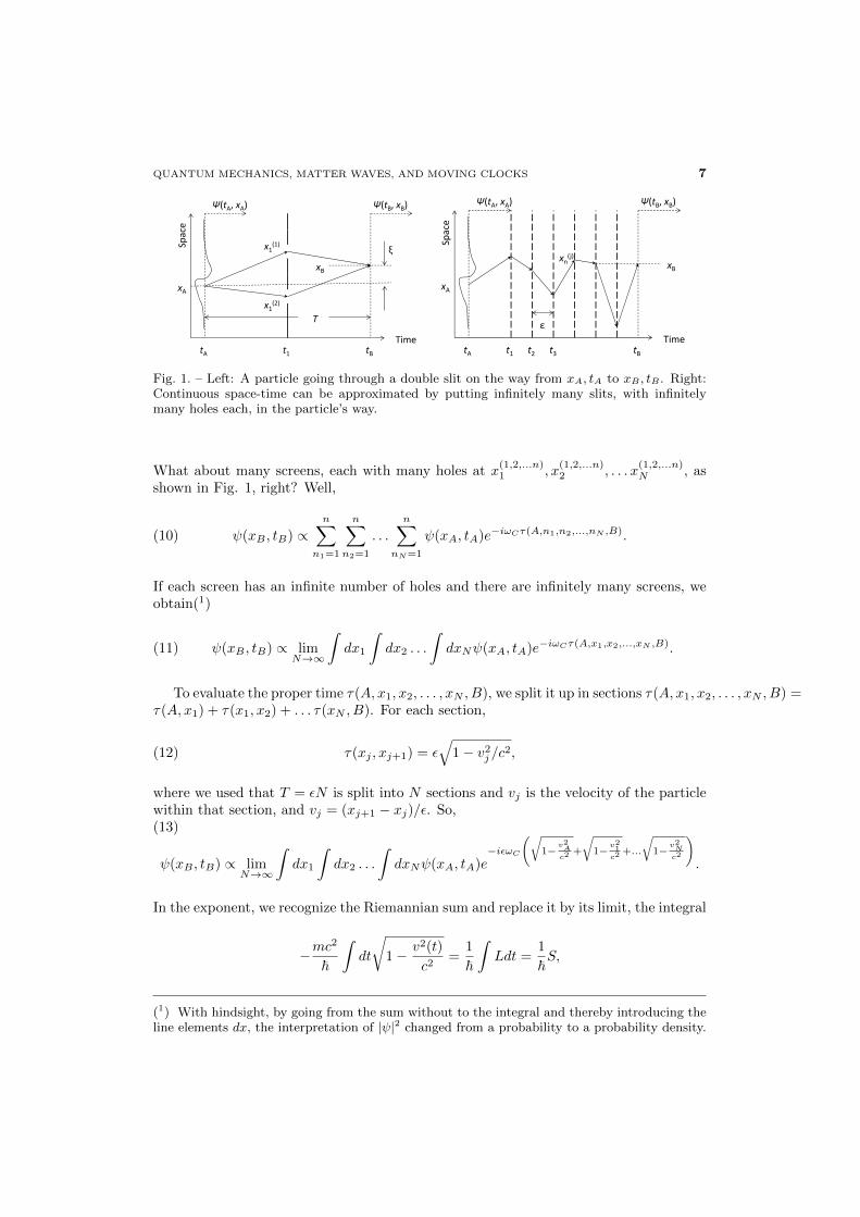
particles, traveling on a straight line at constant velocity. We will gradually extend ourformalism to study a particle in a potential and general trajectories. We assume we knowψ(xA, tA) and want to know ψ(xB , tB), where tB = tA + T and xB = xA + ξ. Take alook at the double-slit experiment shown in Fig. 1, left). At some time t1 between tAand tB , the particle has to pass through holes located at x
(1,2)1 . Clearly, the contribution
of ψ(~xA, tA) to ψ(xB , tB) is given by the sum
(8) ψ(xB , tB) ∝ ψ(xA, tA)(e−iωCτ(A,1,B) + e−iωCτ(A,2,B))
where τ(A, 1, B) is the proper time elapsed on the path from A via 1 to B. The exact
form of it is unimportant for now. If the screen has, say, n holes located at x(1,2,...n)1 , we
obtain
(9) ψ(xB , tB) ∝n∑
n1=1
ψ(xA, tA)e−iωCτ(A,n1,B).
QUANTUM MECHANICS, MATTER WAVES, AND MOVING CLOCKS 7ce
Ψ(tA, xA) Ψ(tB, xB)
Spac
ξ
xB
x1(1)
T
xAx1(2)
TimetA t1 tB
T
ce
Ψ(tA, xA) Ψ(tB, xB)
Spac
xBxn(j)
xA
TimetA t1 t2 t3 tB
ε
Fig. 1. – Left: A particle going through a double slit on the way from xA, tA to xB , tB . Right:Continuous space-time can be approximated by putting infinitely many slits, with infinitelymany holes each, in the particle’s way.
What about many screens, each with many holes at x(1,2,...n)1 , x
(1,2,...n)2 , . . . x
(1,2,...n)N , as
shown in Fig. 1, right? Well,
(10) ψ(xB , tB) ∝n∑
n1=1
n∑n2=1
. . .
n∑nN=1
ψ(xA, tA)e−iωCτ(A,n1,n2,...,nN ,B).
If each screen has an infinite number of holes and there are infinitely many screens, weobtain(1)
(11) ψ(xB , tB) ∝ limN→∞
∫dx1
∫dx2 . . .
∫dxNψ(xA, tA)e−iωCτ(A,x1,x2,...,xN ,B).
To evaluate the proper time τ(A, x1, x2, . . . , xN , B), we split it up in sections τ(A, x1, x2, . . . , xN , B) =τ(A, x1) + τ(x1, x2) + . . . τ(xN , B). For each section,
(12) τ(xj , xj+1) = ε√
1− v2j /c
2,
where we used that T = εN is split into N sections and vj is the velocity of the particlewithin that section, and vj = (xj+1 − xj)/ε. So,(13)
ψ(xB , tB) ∝ limN→∞
∫dx1
∫dx2 . . .
∫dxNψ(xA, tA)e
−iεωC(√
1− v2Ac2
+
√1− v
21c2
+...
√1− v
2Nc2
).
In the exponent, we recognize the Riemannian sum and replace it by its limit, the integral
−mc2
~
∫dt
√1− v2(t)
c2=
1
~
∫Ldt =
1
~S,
(1) With hindsight, by going from the sum without to the integral and thereby introducing theline elements dx, the interpretation of |ψ|2 changed from a probability to a probability density.
8 HOLGER MULLER
where L is the Lagrangian of a point particle in special relativity and S the action. Sowe can write
(14) ψ(xB , tB) ∝ limN→∞
∫dx1
∫dx2 . . .
∫dxNψ(xA, tA) exp
[i
~
∫dtL(x, x)
]or
(15) ψ(xB , tB) =
∫Dxψ(xA, tA) exp
[i
~
∫dtL(x, x)
].
The factor of√
1− v2/c2 in the Lagrangian is nothing but the relationship betweenproper time and coordinate time, L = −mc2dτ/(dt). To include an interaction, we mayuse general relativity (GR), a description of gravity. The relationship between propertime and coordinate time in GR is
(16) dτ =√−gµνdxµdxν/c.
The Lagrangian of a point particle is still L = −mc2dτ/(dt).
1.4. Derivation of the Schrodinger equation. – We shall follow the approach of Feyn-
man [46]. We start by using the action(17)
S = −∫mc2
√−gµνuµuνdt ≈ −
∫mc2
(1− 1
2h00 + h0juj
c− 1
2 (δjk − hjk)uj
c
uk
c
)dt
where we have expanded the square-root to leading order, choosing as a laboratory frameone in which the particle is moving slowly and the gravitational potential is weak.(2)In this frame, uj is the usual 3-velocity. We now compute the path integral for aninfinitesimal time interval t → t + ε and an infinitesimal distance qµ = (xB)µ − (xA)µ.For an infinitesimal ε, we have vj = qj/ε, so
(18) ψ(t+ ε, (xA)j) = N
∫d3q ψ(t, (xA)j − qj)e−i
mc2ε~
(1− 1
2h00
)e−
12Ajkq
jqk+Bjqj
where N is a normalization factor and
(19) Ajk ≡ −im
~ε(δjk − hjk), Bj ≡
imc
~h0j .
We can expand in powers of ε, qµ:
ψ + ε∂tψ(20)
= N
∫d3q
(ψ − qj∂jψ + 1
2qjqk∂j∂kψ
)(1− imc
2ε
~(1− 1
2h00
))exp
[1
2Ajkq
jqk +Bjqj
]
(2) The minus sign of h00 comes from η00 = −1
QUANTUM MECHANICS, MATTER WAVES, AND MOVING CLOCKS 9
where ψ ≡ ψ(t, ~xA). We compute
(21)
∫e−
12Ajkq
jqk+Bjqj
d3q =(2π)3/2
√detA
e−12Bj(A
−1)jkBk ,
where detA is the determinant of A and A−1is the inverse matrix. We obtain
ψ + ε∂tψ = N(2π)3/2
√detA
[(1− imc
2ε
~(1− 1
2h00)
)ψ
−(∂jψ)∂
∂Bj+
1
2(∂j∂kψ)
∂
∂Bj
∂
∂Bk
]exp
(1
2BjBk(A−1)jk
).(22)
The normalization factor is determined from the fact that ψ(t + ε, ~xA) must approachψ(t, ~xA) for ε → 0. We carry out the derivatives. We now neglect all terms that aresuppressed by two powers of 1/c or more, including the hjk terms, and terms proportionalto ε2. This leads to a Schrodinger equation
(23) i~d
dtψ = −mc2 1
2h00ψ −~2
2m
(~∇−m~H
)2
ψ,
where we have substituted ψ → e−iωCtψ. The 3-vector ~H is defined by Hj ≡ (ic/~)h0j .To see that this is the familiar Schrodinger equation, we note that U = −h00c
2/2 is
the scalar gravitational potential. The significance of ~H is a gravitational vector potentialthat describes “frame dragging” for a rotating source mass. This post-Newtonian effectof GR is extremely small on Earth.
From here on, we may derive the entire program of quantum mechanics, e.g., derivethe conservation of the probability current to arrive at a interpretation of the wavefunction, the uncertainty relationship or commutation relations, and generalize the theoryto describe multiple particles. This shows that quantum mechanics is a description ofwaves oscillating at the Compton frequency that explore all possible paths through curvedspacetime.
1.5. Derivation of the Dirac equation without gravity . – The theory still has impor-
tant gaps. We do not know about spin yet, and while we started relativistically, theSchrodinger equation we obtained is only nonrelativistic. It is not straightforward toobtain a relativistic theory in analogy to Eq. (15). The difficulties are substantial, so wewill tackle them for a special relativistic framework, without gravity.
The difficulties arose when integrating the exponential exp(−imc2√
1− v2/c2) overall of space, because there is no limit on the velocity v. In particular, the integrand isnot well behaved when v → c and beyond. One might attempt to cut the integral beforev = c or anywhere else, but this would not lead to a Lorentz-invariant theory. The reasonis that any speed below v = c is the rest frame of a physically possible observer, andcan thus not be excluded from the theory. Cutting at v = c, on the other hand, doesn’tavoid divergence. Our luck in the previous chapter was that paths at and outside thelight cone were suppressed by gaussian functions in the nonrelativistic framework. Butnow that we want to develop the relativistic theory, this is no longer possible. We areled to accept that the divergence is not a computational problem, but an indication thatthe model that we have used so far needs to be refined.
10 HOLGER MULLER
1.5.1. Re-writing the proper time. Since the difficulty arises from the square-root in the
exponential, we shall try to avoid the square root. Using the momentum ~p = ∇~qL = m~vγ
we shall re-write L = ~p · ~q − H. The function H, the Hamiltonian, turns out to beH = mc2γ =
√p2c2 +m2c4. We then use Dirac’s trick of replacing
(24)√p2c2 +m2c4 ≡ c(−~α) · ~p+ βmc2.
In order for this to work, we must require (−~α)2 = 1, β2 = 1, and (−~α)β + β(−~α) = 0.(The sign of α is arbitrary. We choose it to be negative, so that our end result has thefamiliar form.) It is clear that ~α and β cannot be ordinary numbers, but they may be4× 4 matrices, e.g.,
(25) ~α =
(0 ~σ~σ 0
), β =
(1 00 −1
),
where ~σ are the Pauli matrices. We now have
(26) L = ~p · ~q + c~α · ~p−mc2β.
Note that this Lagrangian is a matrix. For now, we shall continue our calculation andinterpret this fact if and when we obtain a result.
We could now try inserting the new Lagrangian into the path integral, Eq. (15)
and use ~p = m~v/√
1− v2/c2. This, however, brings back the square-root and thus anintegrand which is not well-behaved at the light cone. We can, however, generalize thepath integral by treating ~p, ~q as independent variables and integrate over all trajectoriesin phase-space, not just all trajectories in real space. We thus write
(27) ψ(~xB , tB)
∫ D3p1
(2π)3
∫D3x exp
[−i~
∫dt(~p · ~q + c~α · ~p−mc2β
)]ψ(~xA, tA).
1.5.2. Derivation of the Dirac equation. As before, consider an infinitesimal interval
t → t + ε, ~x → ~x + ~q. We may use just one integration each. Noting that ~q = ~q/ε, weobtain
(28) ψ(t+ ε, x) = N
∫d3p
(2π)3
∫d3q exp
[−i~~p · ~q +
iε
~(−c~α · ~p+mc2β
)]ψ(t, ~x− ~q).
We note that∫d3qe−i~p·~q/~ψ(~x− ~q) = −ei~p·~x/~Φ(−~p, t) is given by the momentum-space
wave function Φ(~p, t). Inserting this into the path integral gives
(29) ψ(t+ ε, x) = −N∫
d3p
(2π)3exp
[iε
~(−c~α · ~p+mc2β
)]e−i~p·~x/~Φ(−~p, t).
Since ε is an infinitesimal quantity, we may expand to first order on both sides of theequation:
ψ(t, ~x) + εψ(t, ~x)(30)
= −N∫
d3p
(2π)3e−i~p·~x/~Φ(−~p, t)−N
∫d3p
(2π)3
iε
~(−c~α · ~p+mc2β
)e−i~p·~x/~Φ(−~p, t).
QUANTUM MECHANICS, MATTER WAVES, AND MOVING CLOCKS 11
The first term is the reverse Fourier transform and yields the position-space wave func-tion. We determine the normalization factor by noting that if ε = 0, the right hand sidemust equal the left hand side, i.e., N = −1. The remaining terms are
(31) ψ(t, ~x) =
∫d3p
(2π)3
i
~(−c~α · ~p+mc2β
)e−i~p·~x/~Φ(−~p).
We can replace the ~p in the parenthesis by the derivative −(~/i)~∇ acting on the expo-nential,
(32) i~ψ =
[~ic~α · ~∇+mc2β
]ψ,
the Dirac equation!(3) We have thus arrived at a relativistic wave equation, and discov-ered spin. Our need to introduce the 4× 4 matrices ~α and β means the wave function isa vector having 4 components. We could now derive conserved quantities, find solutionsto the Dirac equation, and recover the Schrodinger equation in the nonrelativistic limit.This would show us that the 4 components of ψ are the particle and antiparticle withspin up and spin down, respectively.
Our notion of an elementary particle as a single clock turned out to be incompatiblewith relativity. Rather, a particle is a set of four clocks, two of which tick forward, twobackward. The 4× 4 langrangian gives the time lags in an experiment comparing any ofthe four to another one.
1.5.3. Interpretation. We now come back to the interpretation: Let us label the spinor
components of ψ by an index s = 1 . . . 4. If a particle is found at four-position xµA in aspin state s, we may call this a spinor event (A, s). The components of the Lagrangian(L)rsdt then represent the phase accumulated by the state between two infinitesimallyseparated spinor events (A, s) and (B, r). The phase is, e.g., φ = (L)1
1ε = (pv +mc2)εfor r = s = 1, (pv − mc2)ε for r = s = 3, and −cpε if r = 3, s = 1, where ε is aninfinitesimal coordinate time interval. To calculate the phases between two events, theevents have to be amended by a discrete coordinate s.
The path integral Eq. (27) is over all of phase space,∫DpDq. Thus, there are
arbitrary combinations of matrices αx, αy, αz in the exponential of one path, e.g., . . .×e−
i~ cαxpxe−
i~ cαzpze−
i~ cαypy×. . . ψ. Since each term with a matrix may change the spin s,
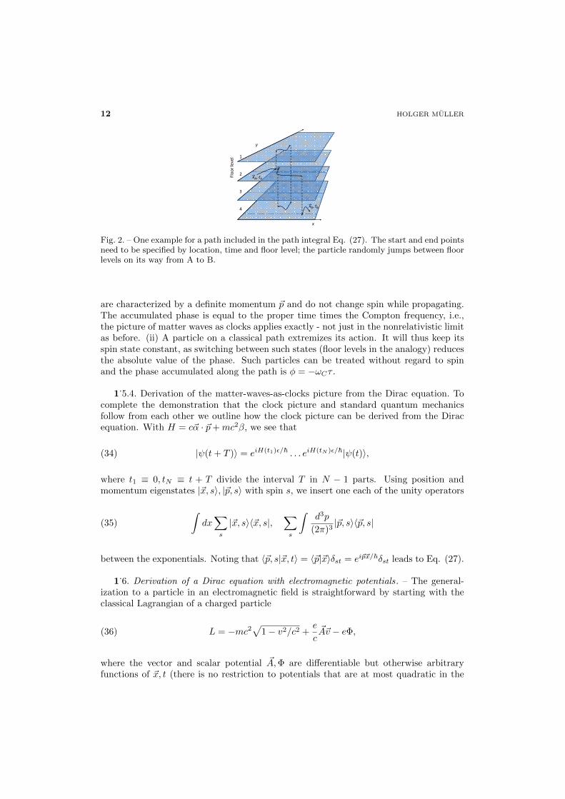
the particle not only takes all possible paths through phase space, but thereby also goesthrough all possible paths through spin space (Fig. 2). Loosely, we may draw an analogybetween the propagation of a Dirac particle and observers carrying clocks on randompaths through a building having four floors in which proper time passes at different rates- forward and backward. In such a building, time, geographical latitude and longitudeA as well as the floor level s constitute a full description of an event (A, s).
We consider two special cases: (i) Eigenstates of L,
(33) eiL/~dtψ = e−iωCdτψ = e−ipµdxµ/~ψ,
(3) I derived this on board the train to Varenna on July 14, 2013.
12 HOLGER MULLER
y
1
or level
2
3
xA, tAFlo
3
4 xB, tB
x
Fig. 2. – One example for a path included in the path integral Eq. (27). The start and end pointsneed to be specified by location, time and floor level; the particle randomly jumps between floorlevels on its way from A to B.
are characterized by a definite momentum ~p and do not change spin while propagating.The accumulated phase is equal to the proper time times the Compton frequency, i.e.,the picture of matter waves as clocks applies exactly - not just in the nonrelativistic limitas before. (ii) A particle on a classical path extremizes its action. It will thus keep itsspin state constant, as switching between such states (floor levels in the analogy) reducesthe absolute value of the phase. Such particles can be treated without regard to spinand the phase accumulated along the path is φ = −ωCτ .
1.5.4. Derivation of the matter-waves-as-clocks picture from the Dirac equation. To
complete the demonstration that the clock picture and standard quantum mechanicsfollow from each other we outline how the clock picture can be derived from the Diracequation. With H = c~α · ~p+mc2β, we see that
(34) |ψ(t+ T )〉 = eiH(t1)ε/~ . . . eiH(tN )ε/~|ψ(t)〉,
where t1 ≡ 0, tN ≡ t + T divide the interval T in N − 1 parts. Using position andmomentum eigenstates |~x, s〉, |~p, s〉 with spin s, we insert one each of the unity operators
(35)
∫dx∑s
|~x, s〉〈~x, s|,∑s
∫d3p
(2π)3|~p, s〉〈~p, s|
between the exponentials. Noting that 〈~p, s|~x, t〉 = 〈~p|~x〉δst = ei~p~x/~δst leads to Eq. (27).
1.6. Derivation of a Dirac equation with electromagnetic potentials. – The general-
ization to a particle in an electromagnetic field is straightforward by starting with theclassical Lagrangian of a charged particle
(36) L = −mc2√
1− v2/c2 +e
c~A~v − eΦ,
where the vector and scalar potential ~A,Φ are differentiable but otherwise arbitraryfunctions of ~x, t (there is no restriction to potentials that are at most quadratic in the
QUANTUM MECHANICS, MATTER WAVES, AND MOVING CLOCKS 13
coordinates as in nonrelativistic path integrals). Proceeding as above, we obtain
~p = γm~v +e
c~A, H =
√(c~p− e ~A)2 +m2c4 + eΦ,
L = ~p · ~q − ~α · (c~p− e ~A)−mc2β − eΦ,(37)
and again calculate a path integral over an infinitesimal interval t→ t+ ε, ~x→ ~x+ ~q, asin Eq. (27). This leads to the Dirac equation
(38) i~ψ =
[c~α ·
(i
~~∇− e
c~A(~x)
)−mc2β − eΦ(~x)
]ψ.
From the basic equations of motion, we could now proceed to construct the theory ofinteracting Fermions, i.e., quantum electrodynamics. Of course, this is a huge undertak-ing, requiring second quantization as a way of dealing with multi-particle systems. Wewill not consider this.
1.7. Derivation of the Dirac equation with gravity, in curved space-time. –
1.7.1. Derivation. The proper time is expressed by the Lagrangian
(39) L =dτ
dt= −mc
√−gµν xµxν .
The momentum is
(40) pµ =∂L
∂xµ= mc
gµν xν√
−gµν xµxν
and satisfies
(41) gκλpκpλ = m2c2gκλgκν x
νgλµxµ
−gµν xµxν= −m2c2.
We note that
(42) pµxµ − L = mc
gµν xν xµ√
−gµν xµxν− L = 0.
Now we work in a specific frame and use
(43) H = pkxk − L = pµx
µ − p0x0 − L = −p0x
0 = −p0c = −c√p2
0.
From Eq. (41), we obtain
(44) −m2c2 = gµνpµpν = g00p0p0 + 2g0jp0pj + gjkpjpk,
which we may solve for p20 and insert:
(45) H = c
√1
−g00(m2c2 + 2g0jp0pj + gjkpjpk)
14 HOLGER MULLER
At this point, let us define
(46) gµν =gµν
−g00, m2 =
m2
−g00.
So that
(47) H = c√m2c2 + 2g0jp0pj + gjkpjpk.
In flat spacetime, this reduces to√p2c2 +m2c4 as it should. We note that p0 = −H/c
under the square-root, so we have H on the right hand side and the left hand side,
(48) H2 = m2c4 + 2cg0jpjH + c2gjkpjpk.
We obtain
(49) H = cg0jpj ± c√
(g0j g0k + gjk)pjpk + m2c2.
We pick the plus sign so the Hamiltonian reduces to the usual one in flat space-time. Wenow introduce a dreibein daj so that
(50) g0j g0k + gjk = djadkbηab = djad
kb δab.
We define
(51) αj = djaαa,
where α1,2,3 are the familiar Dirac matrices. It is easy to check that
αj , αk = djadkb (αaαb + αbαa) = 2djad
kb δab = 2(g0j g0k + gjk)
αj , β = dja(αaβ + βαa) = 0.(52)
where a, b = ab+ ba denotes the anticommutator. Thus,
(αjpj + βmc
)2= αjαkpjpk + (αjβ + βαj)pjmc+ β2m2c2
= 12 (αjαk + αkαj)pjpk + β2m2c2
= (g0j g0k + gjk)pjpk + m2c2.(53)
So we define
(54) L = pkqk − cg0j(xk, t)pj − c
[(−αj(xk, t))pj + βm(xk, t)c
]where we have explicitly denoted that the α and m depend on the coordinate and thetime. (As before, the sign before αj is arbitrary and chosen such that the end result
QUANTUM MECHANICS, MATTER WAVES, AND MOVING CLOCKS 15
will reduce to the familiar Dirac equation in flat space time.) If all that works, our pathintegral will be
ψ(t+ T ) =
∫ D3p
(2π)3√−g
∫D3x√−g
× exp
∫ [− i~pkq
k +ic
~g0jpj −
ic
~(−αjpj + βmc
)]dt
ψ(t, ~x).
(55)
As before, we calculate an infinitesimal step
(56) ψ(~x, t+ ε) =
∫d3p
(2π)3√−g
∫d3q√−ge− i
~pkqk
eic~ εg
0jpje−ic~ ε[−αjpj+βmc]ψ(~x− ~q, t).
Just as in the case without gravity, we are allowed to evaluate√−g, g, m at ~x instead of
~x− ~q. That leaves us with
ψ(~x, t+ ε) =
∫d3p
(2π)3eic~ εg
0jpje−ic~ ε[−αjpj+βmc]
∫d3qe−
i~pkq
k
ψ(~x− ~q, t)
=
∫d3p
(2π)3eic~ εg
0jpje−ic~ ε[−αjpj+βmc]e−
i~pkx
k
Φ(−~p, t)(57)
We use ψ(~x, t+ ε) = ψ(~x, t) + εψ(~x, t) on the left hand side and obtain
i~ψ = −∫
d3p
(2π)3c(g0jpj −
[−αjpj + βmc
])e−
i~pkx
k
Φ(−~p, t)
=
[~i
(αj − g0j
)∂j + βmc2
] ∫d3p
(2π)3e−
i~pkx
k
Φ(−~p, t).(58)
We are now able to write the Dirac equation in curved space-time in compact form
(59) i~ψ =
[~i
(αj − g0j
)∂j + βmc2
]ψ,
where the barred symbols are defined by
(60) αj , αk = 2(gµν + g0j g0k), αj , β = 0, gµν =gµν
−g00, m =
m√−g00
.
The α can be constructed from the standard Dirac matrices using the dreibein, as ex-plained above. This Dirac equation describes the propagation of relativistic particleswith spin through gravitational fields, which may be arbitrarily strong. Note that it hasbeen derived from the picture of the matter wave as a clock, the way we derived theflat-space time Dirac eqution before.
16 HOLGER MULLER
1.7.2. A simple limiting case. In the weak-gravity limit, we have gµν = ηµν +hµν with
|h00| 1 and h0j = hjk = 0. Thus, the dreibein satisfies
(61)1
−g00δjk = djad
kb δab
so we may choose dja = δja/√−g00. Thus, our Dirac equation reduces to
(62) i~ψ =
[~
i(1− 12h
00)αj∂j + βmc2 + 1
2βh00mc2
]ψ
For a particle with low momentum, 12βh00mc
2 appears like a scalar potential. Newtonianmechanics, here we come. The β in that potential makes sure that antimatter fallsdownward, another nice feat. An alternative way of writing this
(63) i(1− 12h
00)ψ =
[1
iαj∂j + βωC
]ψ
reveals once more that gravity in quantum mechanics is described by the gravitationalredshift to the Compton frequency.
1.7.3. Comparison to the usual form. The Dirac equation in curved space time found
in the literature [49] is sometimes called the tensor representation of the Dirac equation(TRD) [50]. It reads
(64) [i~eµαγα(∂µ − Γµ)−mc]ψ = 0
where
(65) Γµ =i
4σαβ [eaν∂µe
νb + eaνeσbΓνσµ]
is the spin connection, which is not a tensor. Our Dirac equation, on the other hand,does not have a spin connection and thus belongs to the Quadruplet Representation ofthe Dirac theory (QRD − 0) in which eµαγ
αΓµ = 0. It was recently shown that in anopen neighborhood of each spacetime point, every TRD equation is in fact equivalent toa QRD equation and vice versa. This holds under “mild assumptions” on the metric, theGodel universe being a notable exception [50]. We can use eµαγ
αΓµ = 0 in Eq. (64) andre-write is as
(66) i~e0αγ
αψ = −i~ekαγα∂kψ +mcψ.
We multiply both sides with e0βγ
β
(67) −i~g00ψ = −i~e0βekαγ
αγβ∂kψ + e0βγ
βmcψ
Let’s consider the first term on the right hand side:
(68) e0βekαγ
αγβ =1
2(e0βekαγ
αγβ + e0αekβγ
βγα) =1
2(e0βekαγ
αγβ + 2e0αekβη
αβ − e0αekβγ
αγβ).
QUANTUM MECHANICS, MATTER WAVES, AND MOVING CLOCKS 17
Note that the definition of the vierbein involves six unphysical degrees of freedom. Theyare three Lorentz boosts and three rotations. If we use the three Lorentz boosts to set
(69) e0a = 0 (for a 6= 0),
we obtain
(70) e0βekαγ
αγβ =1
2(e0
0ekαγ
αγ0 − 2e00ek0 − e0
0ekβγ
0γβ) = −e00ekaα
a − e00ek0 ,
where we used
(71) γ0 ≡ β, γk ≡ γ0αk, αaβ = −βαa, γaγ0 = γaβ = βαaβ = −αa.
We also use
(72) e0βγ
β = e00β + e0
bγb = e0
0β
to bring the Dirac equation into the form
(73) −i~g00ψ = i~(e00ekaα
a + e00ek0)∂kψ + e0
0βmcψ.
We can replace e00ek0 by the metric, since
(74) g0k = e0αekβη
αβ = e00ekβη
0β = e00ek0 .
Therefore,
(75) i~ψ =
[~i
(ak − g0k
)∂k −
e00βmc
g00
]ψ
where
(76) a =e0
0ekaα
a
g00.
It remains to show that the α satisfy the anticommutator Eq. (60). This can be doneby calculating
(g00)2aj , ak = (e00)2ekae
jb(α
aαb + αbαa) = 2(e00)2ekae
jbηab
= 2(e00)2[ekαe
jβη
αβ − ek0ej0η00 − ek0ejbη0b + ekaej0ηa0] = 2(e0
0)2[gkj + ek0ej0](77)
and
g0jg0k = e0αejβe
0γekδηαβηγδ = (e0
0)2ej0ek0 .(78)
Finally, inserting e00 =
√−g00 brings the standard form of the Dirac equation into the
form that we derived from the path integral, Eq. (59). Our equation and the standardform are equivalent.
18 HOLGER MULLER
1.8. Discussion. – Assuming that the phase accumulated by a matter wave packet
is always proportional to the Compton frequency times the proper time measured alongthe path taken by the wave packet, we have derived the equations of motion of quantummechanics. Our results hold for gravitational fields of any strength, wave packets of anyspeed, and with or without spin (the case of a spinless particle can be derived by iteratingthe Dirac equation). Note that all Lagrangians we have used are more or less complicatedrestatements of the Compton frequency times the proper time, for eigenfunctions of theLagrangian. There is no exception to the rule that “rocks” (massive wave packets) areclocks.
1.9. Review of some counterarguments. – Having completed our demonstration, we
briefly revisit some arguments that have been raised against the “clock picture.” In partic-ular, we examine those arguments that reject the notion that wave-packets in matter-waveinterferometers can be treated like two clocks that measure the proper time differencealong two trajectories. Those who make these arguments find support in the fact thatthe phase of a matter-wave interferometer can be determined in a representation-free(with respect to the wave-packets position or momentum) formalism [42, 43], withoutexplicit reference to the gravitational redshift, Compton frequency, or the proper timein the non-relativistic limit [39], and that for some interferometer geometries, the freeevolution phase difference accumulated by wave-packets traveling along different arms ofthe interferometer is zero [40, 39, 45]. While these points are technically correct, they donot refute the clock picture, as they are all based on the Schrodinger/Dirac formulationof quantum mechanics, which we have shown can be derived from the clock picture.
1.10. Conclusion. – In general relativity, the trajectory of a freely falling test particle
is the one that leads to extremal proper time τ . The phase accumulated by a wave packettraveling between events A and B is given by the proper time elapsed along its path
(79) φclock = ωclockτAB ,
where ωclock is the frequency of the clock in its own rest frame. The path of a matterwave packet is determined from the same principle of least action, and its phase given by
(80) φ = −ωCτAB ,
and hence identical (equal and opposite) to the one of a clock ticking at the particle’sCompton frequency. For free Dirac particles, these statements apply exactly to semiclas-sical states as well as to eigenspinors of L (or L in curved space-time). We deriveda path integral for the Dirac equation in which particles explore all paths in real space,momentum space, and spin space by starting only from a simple and easily motivatedLagrangian, −mc2dτ/dt, and the requirement that the theory be Lorentz invariant.
Dirac’s trick is used as one of several mathematical devices to avoid the square-rootin the action without changing the action, requiring the addition of unphysical degreesof freedom, or simply squaring the action. Note this led naturally to fermions, whereaswe have not found a way to treat bosons directly (it is possible to find a Klein-Gordonequation by iterating the Dirac equation). The restriction of path integrals to potentialsthat are at most quadratic in the coordinates is lifted and thus found to be an artifact ofnonrelativistic physics. We also found an intuitive analogy between Dirac particles andpaths in a building. We may conclude that matter waves can be exactly treated as clocks.
QUANTUM MECHANICS, MATTER WAVES, AND MOVING CLOCKS 19
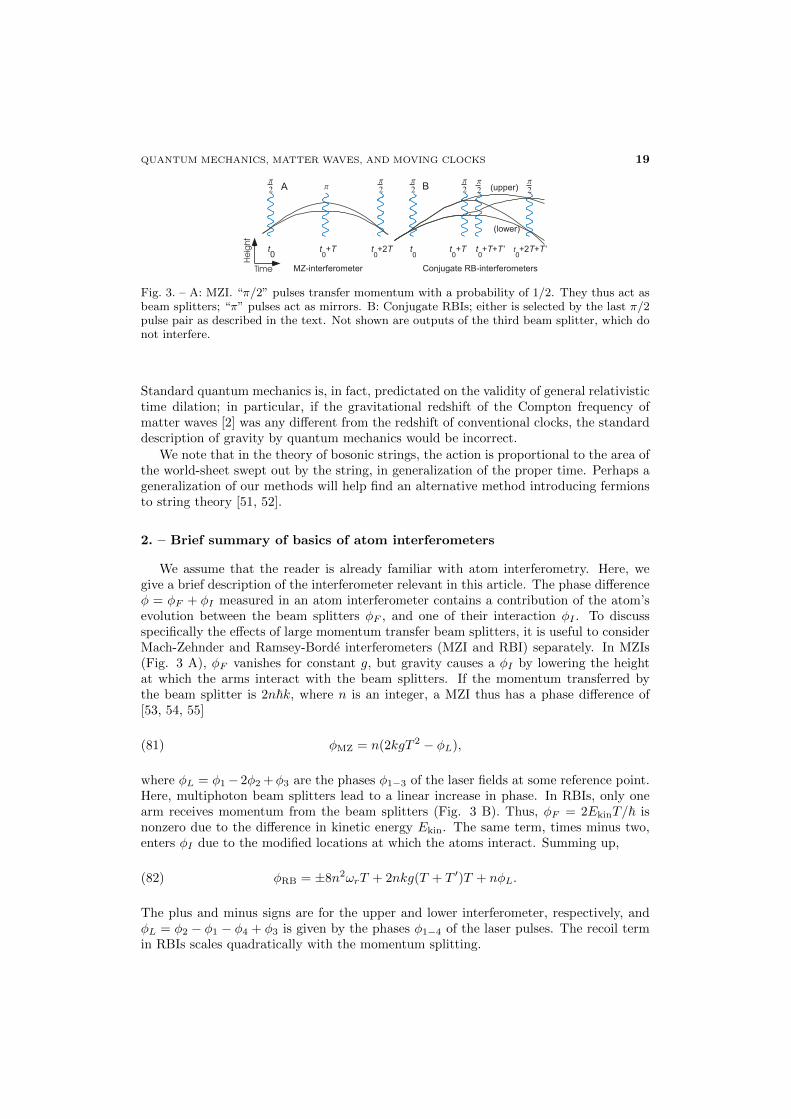
Fig. 3. – A: MZI. “π/2” pulses transfer momentum with a probability of 1/2. They thus act asbeam splitters; “π” pulses act as mirrors. B: Conjugate RBIs; either is selected by the last π/2pulse pair as described in the text. Not shown are outputs of the third beam splitter, which donot interfere.
Standard quantum mechanics is, in fact, predictated on the validity of general relativistictime dilation; in particular, if the gravitational redshift of the Compton frequency ofmatter waves [2] was any different from the redshift of conventional clocks, the standarddescription of gravity by quantum mechanics would be incorrect.
We note that in the theory of bosonic strings, the action is proportional to the area ofthe world-sheet swept out by the string, in generalization of the proper time. Perhaps ageneralization of our methods will help find an alternative method introducing fermionsto string theory [51, 52].
2. – Brief summary of basics of atom interferometers
We assume that the reader is already familiar with atom interferometry. Here, wegive a brief description of the interferometer relevant in this article. The phase differenceφ = φF + φI measured in an atom interferometer contains a contribution of the atom’sevolution between the beam splitters φF , and one of their interaction φI . To discussspecifically the effects of large momentum transfer beam splitters, it is useful to considerMach-Zehnder and Ramsey-Borde interferometers (MZI and RBI) separately. In MZIs(Fig. 3 A), φF vanishes for constant g, but gravity causes a φI by lowering the heightat which the arms interact with the beam splitters. If the momentum transferred bythe beam splitter is 2n~k, where n is an integer, a MZI thus has a phase difference of[53, 54, 55]
(81) φMZ = n(2kgT 2 − φL),
where φL = φ1− 2φ2 +φ3 are the phases φ1−3 of the laser fields at some reference point.Here, multiphoton beam splitters lead to a linear increase in phase. In RBIs, only onearm receives momentum from the beam splitters (Fig. 3 B). Thus, φF = 2EkinT/~ isnonzero due to the difference in kinetic energy Ekin. The same term, times minus two,enters φI due to the modified locations at which the atoms interact. Summing up,
(82) φRB = ±8n2ωrT + 2nkg(T + T ′)T + nφL.
The plus and minus signs are for the upper and lower interferometer, respectively, andφL = φ2 − φ1 − φ4 + φ3 is given by the phases φ1−4 of the laser pulses. The recoil termin RBIs scales quadratically with the momentum splitting.
20 HOLGER MULLER
gx2
x
+v
‐v0x2
A B C
x
2 +v0
+v0+v0
x1
x4x1
Time
T T Tx3
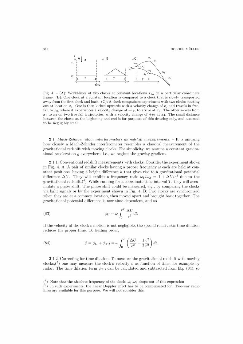
Fig. 4. – (A): World-lines of two clocks at constant locations x1,2 in a particular coordinateframe. (B): One clock at a constant location is compared to a clock that is slowly transportedaway from the first clock and back. (C): A clock-comparison experiment with two clocks startingout at location x1. One is then kicked upwards with a velocity change of v0 and travels in free-fall to x2, where it experiences a velocity change of −v0, to arrive at x3. The other moves fromx1 to x3 on two free-fall trajectories, with a velocity change of +v0 at x4. The small distancebetween the clocks at the beginning and end is for purposes of this drawing only, and assumedto be negligibly small.
2.1. Mach-Zehnder atom interferometers as redshift measurements. – It is amusing
how closely a Mach-Zehnder interferometer resembles a classical measurement of thegravitational redshift with moving clocks. For simplicity, we assume a constant gravita-tional acceleration g everywhere, i.e., we neglect the gravity gradient.
2.1.1. Conventional redshift measurements with clocks. Consider the experiment shown
in Fig. 4, A. A pair of similar clocks having a proper frequency ω each are held at con-stant positions, having a height difference h that gives rise to a gravitational potentialdifference ∆U . They will exhibit a frequency ratio ω1/ω2 = 1 + ∆U/c2 due to thegravitational redshift.(4) While running for a coordinate time interval T , they will accu-mulate a phase shift. The phase shift could be measured, e.g., by comparing the clocksvia light signals or by the experiment shown in Fig. 4, B: Two clocks are synchronizedwhen they are at a common location, then moved apart and brought back together. Thegravitational potential difference is now time-dependent, and so
(83) φU = ω
∫ T
0
∆U
c2dt.
If the velocity of the clock’s motion is not negligible, the special relativistic time dilationreduces the proper time. To leading order,
(84) φ = φU + φTD = ω
∫ T
0
(∆U
c2− 1
2
v2
c2
)dt.
2.1.2. Correcting for time dilation. To measure the gravitational redshift with moving
clocks,(5) one may measure the clock’s velocity v as function of time, for example byradar. The time dilation term φTD can be calculated and subtracted from Eq. (84), so
(4) Note that the absolute frequency of the clocks ω1, ω2 drops out of this expression(5) In such experiments, the linear Doppler effect has to be compensated for. Two-way radiolinks are available for this purpose. We will not consider this.
QUANTUM MECHANICS, MATTER WAVES, AND MOVING CLOCKS 21
that a measurement of the gravitational redshift φU is obtained as φU = φ− φTD. Thisis the basic principle of, e.g., gravity-probe B and other experiments with spaceborneclocks [61].
2.1.3. Experiment with piecewise freely falling clocks. Consider the slightly more com-
plicated clock-comparison experiment shown in Fig. 4, C. The clocks are initially syn-chronized at a common location and made to take two different paths by kicking (sitvenia verbo) in intervals T . Each kick provides a velocity change by v0. The clocks arecompared after their paths merge at t = 2T .(6) We can easily generalize Eq. (84) tocalculate the phase difference shown by the clocks:(7)
(85) φ = ω
∫ 2T
0
(∆U
c2− 1
2
v21 − v2
2
c2
)dt.
To subtract the time dilation term, we can monitor the trajectories as before. Under ourassumptions of free fall with a constant gravitational acceleration, there is, however, asimpler method. The time dilation phase equals
(86) φTD = − ω
2c2
∫ 2T
0
(v2
1 − v22
)dt = −ωv0
c2gT 2 = ω
v0
c2(x1 − x2 + x3 − x4),
where we labeled the coordinates of the turning points as in Fig. 4 C. It is thus sufficientto measure the coordinates of the turning points. We have only assumed that Newtonianmechanics is valid and that the clocks are falling with a constant acceleration of free fallthat is identical for both clocks. We did not make any assumptions about the originor magnitude of g.(8) We now have a strategy for our redshift experiment with clocks:send the clocks on the trajectories given in Fig. 4 C and measure the total phase shift φaccumulated between them. Also measure x1−4 and recover the redshift phase as
(87) φU = φ− ωv0
c2(x1 − x2 + x3 − x4).
2.1.4. Comparison to atom interferometer. The clock-comparison experiment has an
exact correspondence to a Mach-Zehnder atom interferometer. The free evolution of thewave packets yields a phase shift in analogy to the one between the clocks in the aboveexperiment, if the clock frequency is replaced by the Compton frequency:
(88) φF = −ωC∫ 2T
0
(∆U
c2− 1
2
v21 − v2
2
c2
)dt
(6) Several other versions of this experiment are possible, for example one in which both clocksare kicked two times each, or one in which the lower clock is kicked three times. The readeris invited to verify that the results of this chapter apply to any of these configurations, as wellas to different initial locations and velocities of the two clocks, so long as the clocks are in thesame position and same velocity as each other initially and finally.(7) We assume that the velocity change does not perturb the operation of the clock so that theclocks are perfect realizations of proper-time measurements.(8) The reader is invited to verify that the above results hold for arbitary initial positions andinitial velocities.
22 HOLGER MULLER
As before, φF = φU + φTD can be decomposed into the redshift part φU and the timedilation φTD which can be expressed as
(89) φTD = −ωCv0
c2(x1 − x2 + x3 − x4).
In an atom interferometer, the velocity changes by v0 is provided by laser-atom interac-tions. For a laser with wavenumber k, the recoil velocity is vr = n~k/m, where n is thenumber of photons that the atom interacts with. Inserting ωC = mc2/~ and v0 = n~k/m,we obtain
(90) φTD = −nk(x1 − x2 + x3 − x4).
The laser-atom interaction also imparts a phase to the matter wave, φI: Whenever aphoton is absorbed, its phase is added to the matter wave. When a photon is emitted,its phase is subtracted. As the photons propagate by a distance x, they accumulate aphase kx.(9) Referring to Fig. 4 C, phase is imparted on the upper wave packet threetimes: A phase +nkx1 at t = 0; a phase −nkx2 at t = T (the negative sign arises becausethe atom is kicked down at this point), and a phase +nkx3 at t = 2T . The lower atomreceived a phase shift of +nkx4 at t = T . Taking the difference between the total phasesimparted by the laser on the upper and lower path, respectively, the laser phase evaluatesto
(91) φI = nk(x1 − x2 + x3 − x4).
So we see that φTD + φI = 0, i.e., the laser phase acts like a laser-based tracker forthe atoms position that automatically adds a counterterm that cancels the time dilationphase. This means, the atom interferometer is in every respect analogous to a redshiftmeasurement using a pair of clocks on the trajectories shown in Fig. 4 C. As before,our only assumptions were freely falling motion with a constant acceleration of arbitrarymagnitude or origin, and an arbitrary initial velocity.
2.1.5. Examples where interpretations as force measurements fail. As is well-known,
the free evolution phase φfree = 0 for the above situation of freely falling wave packets.It is tempting to generalize this notion and assert that it is always true, ignoring thefact that atom interferometers fundamentally measures potentials. This would mean theatom interferometer measures nothing but the physical acceleration of the trajectory ofthe atoms relative to the reference plane used in defining the laser phase [39]. However,if the physical acceleration is modified without changing the potential difference betweenthe paths, the interferometer will not register the change; if the potential difference ischanged without changing the acceleration, the interferometer will. These observationsare inconsistent with an interpretation of the interferometer as a pure accelerometer, butconsistent with an interpretation as a redshift measurement.
Consider, for example, the interferometer shown in Fig. 5, left. It has the sametrajectories as a conventional Mach-Zehnder, except that a common force is applied tothe two wave packets so that the acceleration is not g but can have any value. The
(9) For the following calculation, we shall refer all photon phases to the location x = 0, thoughother conventions would lead to the same result.
QUANTUM MECHANICS, MATTER WAVES, AND MOVING CLOCKS 23
AI phase independent of external imotion
a=0 Ch tia=0 • Change motion• NO global potential -Fz• Matter waveguides, optical latticesFree-fall paths lattices, … • Keep separation the same
a>g • These three interferometers have the same phase
=>Mach-Zehnder atom interferometer is NOT measuring the physical acceleration
These three interferometers have the
Ch it ti l
Compensation mass
• Change gravitational potential by masses• Arranged so that F=0Co-moving mass
RGMU /−=
Free-fall trajectories
Moving This interferometer’s phaseproportional to redshift
compensation mass
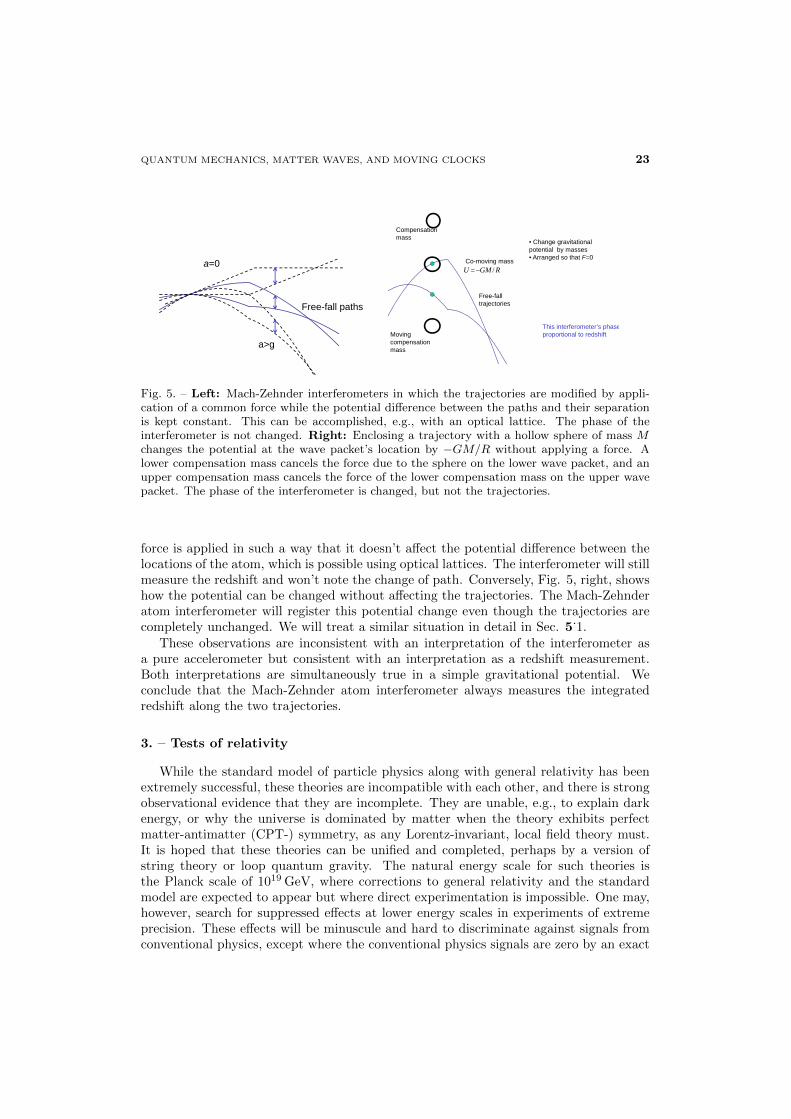
Fig. 5. – Left: Mach-Zehnder interferometers in which the trajectories are modified by appli-cation of a common force while the potential difference between the paths and their separationis kept constant. This can be accomplished, e.g., with an optical lattice. The phase of theinterferometer is not changed. Right: Enclosing a trajectory with a hollow sphere of mass Mchanges the potential at the wave packet’s location by −GM/R without applying a force. Alower compensation mass cancels the force due to the sphere on the lower wave packet, and anupper compensation mass cancels the force of the lower compensation mass on the upper wavepacket. The phase of the interferometer is changed, but not the trajectories.
force is applied in such a way that it doesn’t affect the potential difference between thelocations of the atom, which is possible using optical lattices. The interferometer will stillmeasure the redshift and won’t note the change of path. Conversely, Fig. 5, right, showshow the potential can be changed without affecting the trajectories. The Mach-Zehnderatom interferometer will register this potential change even though the trajectories arecompletely unchanged. We will treat a similar situation in detail in Sec. 5
.1.
These observations are inconsistent with an interpretation of the interferometer asa pure accelerometer but consistent with an interpretation as a redshift measurement.Both interpretations are simultaneously true in a simple gravitational potential. Weconclude that the Mach-Zehnder atom interferometer always measures the integratedredshift along the two trajectories.
3. – Tests of relativity
While the standard model of particle physics along with general relativity has beenextremely successful, these theories are incompatible with each other, and there is strongobservational evidence that they are incomplete. They are unable, e.g., to explain darkenergy, or why the universe is dominated by matter when the theory exhibits perfectmatter-antimatter (CPT-) symmetry, as any Lorentz-invariant, local field theory must.It is hoped that these theories can be unified and completed, perhaps by a version ofstring theory or loop quantum gravity. The natural energy scale for such theories isthe Planck scale of 1019 GeV, where corrections to general relativity and the standardmodel are expected to appear but where direct experimentation is impossible. One may,however, search for suppressed effects at lower energy scales in experiments of extremeprecision. These effects will be minuscule and hard to discriminate against signals fromconventional physics, except where the conventional physics signals are zero by an exact
24 HOLGER MULLER
symmetry of the standard model. Examples for such symmetries are Lorentz and CPTsymmetry. The numerous and extremely sensitive experimental searches for violationsof them in flat space-time, however, have invariably failed to detect anomalies [56]. Bycomparison, the Einstein Equivalence Principle (EEP) [57] is a much less comprehensivelytested symmetry and thus one of the most promising areas for finding low-energy signalsof Planck-scale physics [58].
The EEP is the basis of gravitational theory [59, 60, 4] and holds that gravity affectsall matter in exact proportion to its mass-energy: all objects experience the same accel-eration of free fall g, all clocks experience the same gravitational time dilation, and thelaws of special relativity hold locally in inertial frames. Experimental tests of Lorentzinvariance [56], local position invariance [61], and the weak equivalence principle (WEP)[62] have shown that nature adheres closely to this principle. If the EEP doesn’t hold,general relativity cannot be valid. The EEP is or may be violated in many theoriesthat attempt to join gravity with the standard model of particle physics - e.g., stringtheory, loop quantum gravity, higher dimensions, brane worlds - through new fields suchas dilatons and moduli, or effective friction caused by quantum space-time foam.
3.1. The standard model extension. – The significance of equivalence principle tests
has been studied in the well-known parameterized post-Newtonian framework [60] andothers [33, 58, 63]. The gravitational standard model extension (SME) [64, 65, 66, 67]offers important advantages: It is comprehensive, as it contains all known particles andinteractions; it is consistent, as it preserves desirable features of the standard modelsuch as conservation laws and the existence of a well-behaved flat space-time quantumfield theory; it is predictive, as it can in principle describe the outcome of any experi-ment without any additional assumptions. It provides the most general way to describeLorentz- and EEP-violations that preserves the above features and is in extensive use[56].
The SME is formulated from the standard model Lagrangian by adding all Lorentz- orCPT violating terms that can be formed from known fields and Lorentz tensors. DifferentEEP tests will couple to different combinations of gravitational SME parameters. Usingthe standard model extension [65, 67] as a theoretical framework, we can answer, e.g.,the following questions:
• Which parameters entering fundamental theories will a particular experiment mea-sure? What influences the selection of the best species, like Rb/K or Rb/Rb? Canthe Sun’s gravitational field be used to perform additional measurements? Howmuch will an experiment improve the overall constraints on equivalence principleviolations? What are the implications for antimatter?
• What is the significance of quantum tests of the equivalemce principle relative totests using classical matter? Does gravity couple differently to particles of differentspin? Or to particles exhibiting spin-orbit coupling?
• How will use of species with different nuclear structure enhance the significance ofparticular tests?
• What signals, if any, arise from the nonlinearity of general relativity? Does thevalidity of the EEP for particles in one rest frame guarantee its validity in framesin relative motion? Does its validity at one point imply its validity everywhere?
QUANTUM MECHANICS, MATTER WAVES, AND MOVING CLOCKS 25
3.1.1. The Fermionic sector. The SME is constructed from the Lagrangians of the
standard model and gravity by adding new interactions that violate Lorentz invarianceand the Einstein Equivalence Principle. The non-gravitational Lagrangian density of aDirac particle in the SME is
L =i
2ψΓµ
↔Dµψ − ψMψ,
M = m+ aµγµ + bµγ
5γµ + 12Hµνσ
µν ,
Γν = γν + cµνγµ + dµνγ5γ
µ + eν + ifνγ5 + 1
2gλµνσλµ.(92)
We use a species specific notation (aw)µ, (bw)µ, . . ., where w can take the values n, p, and
e denoting the neutron, the proton, and the electron, respectively. The Lorentz-violatinginteractions are encoded in eight Lorentz tensors a−H known collectively as coefficientsfor Lorentz violation. Most of them lead to observable effects in flat space-time andhave been constrained experimentally to levels well below those relevant here. The aµ
vector, however, can be removed from the flat space time equations of a single fermionvia a redefinition of the energy scale and is unobservable. It becomes observable througheffects in gravitational physics and is thus of particular interest.
The weak gravitational fields in the solar system can be described by a perturbationhµν to Minkowski spacetime. The perturbation is a function of the coefficients aµ −Hµν , via their contribution to the stress-energy tensor. If, in addition, any of thesecoefficients has a non-metric coupling to gravity, those coefficients also become functionsof hµν . In particular, aµ = aµ + aµ becomes the sum of its value in flat space-time aµand a gravitationally-induced fluctuation aµ (here, ’fluctuation’ designates the changewith gravitational potential, not random fluctuations) [67]. Although a nonzero aµ isunobservable on its own, the fluctuation aµ induced by a non-metric coupling to gravityis observable.
For matter that is not spin-polarized, the a- and c-coefficients constitute a full de-scription of EEP violation. For weak gravitational fields and slowly moving objects,it is sufficient to work with the temporal 0 and 00-components. This leaves six mea-surable coefficients (ap)0, (a
n)0, (ae)0, (c
p)00, (cn)00, and (ce)00. These violations of the
EEP affect the free-fall trajectory for particles, as well as the phase shift S/~ to thestate of a quantum particle propagating along that (modified) trajectory, where S isthe action. The c-coefficients also change the binding energy of a composite particle,causing a position-dependence in the effective particle mass. These three effects combineto determine the leading order signal for atom interferometers [3, 68]. The effects ina particular experiment are set by the composition of the atoms in terms of protons,neutrons, and electrons, as well as by their inner structure, which determines how muchthe binding energy is affected by EEP-violation. The effects of the (aw)0 are CPT-odd,or opposite for matter and antimatter, the effects of (cw)00 are CPT-even. This meansthat experiments, despite using normal matter, will also be able to constrain anomalousphysics of antimatter.
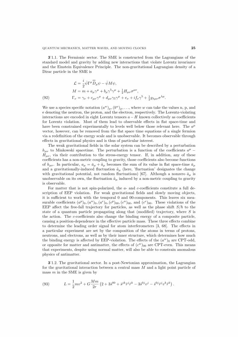
3.1.2. The gravitational sector. In a post-Newtonian approximation, the Lagrangian
for the gravitational interaction between a central mass M and a light point particle ofmass m in the SME is given by
(93) L =1
2mv2 +G
Mm
2r
(2 + 3s00 + sjkrj rk − 3s0jvj − s0j rjvkrk
).
26 HOLGER MULLER
For simplicity, we have taken M to be at rest. We denote ~r the separation between Mand m, pointing towards m. The indices j, k denote the spatial coordinates, ~v the relativevelocity, and r = ~r/r. The components of sµν = sνµ specify Lorentz violation in gravity.If they vanish, LLI is valid.
In principle, the components of s can be defined in any inertial frame of reference.For experiments on Earth (as well as on satellites), it is convenient to choose a Sun-centered celestial equatorial reference frame [69]. The derivation of the time-dependentmodulations of g for an observer on Earth involves taking into account the rotation andorbit of the Earth; the Earth itself is modeled as a massive sphere having a sphericalmoment of inertia of I⊕ ≈ M⊕R2
⊕/2 [60] (not to be confused with the conventionalmoment of inertia, which for Earth is about M⊕r2
⊕/3). It suffices to consider the firstorder in the Earth’s orbital velocity V⊕ ' 10−4c. Bailey and Kostelecky [70] have studiedthis in detail, and we refer the reader to this reference for the detailed signal componentsin the purely gravitational sector.
3.1.3. Electromagnetic sector. An atom interferometer us also sensitive to Lorentz
violation in the physics of electromagnetic fields, as it may cause variations of keff . Thisphysics is described by the Lagrangian density for the electromagnetic sector of the SME,
(94) L = −1
4FµνFµν −
1
4(kF )κλµνF
κλFµν ,
where Fµν is the electromagnetic field tensor. The second term is proportional to adimensionless tensor (kF )κλµν , which vanishes, if Lorentz invariance holds on electrody-namics. The tensor has 19 independent components. The Maxwell equations in vacuumthat are derived from the Eq. (94) read
(95) ∂αFαµ + (kF )µαβγ∂
αF βγ = 0, ∂µFµν = 0,
where
(96) Fµν =1
2εµναβFαβ .
They can be written in a 3+1 decomposition in analogy to the Maxwell equations inanisotropic media [69]. Lorentz violation in electrodynamics is thus analogous to elec-trodynamics in anisotropic media. It is convenient to define the linear combinations
(κDE)jk = −2(kF )0j0k, (κHB)jk = 12εjpqεkrs(kF )pqrs,
(κDB)jk = (kF )0jpqεkpq, (κHE)kj = −(κDB)jk
and
(κe+)jk =1
2(κDE + κHB)jk, (κo+)jk =
1
2(κDB + κHE)jk, κtr =
1
3(κDE)ll.
(κe−)jk =1
2(κDE − κHB)jk − 1
3δjk(κDE)ll, (κo−)jk =
1
2(κDB − κHE)jk.(97)
The ten degrees of freedom of κo− and κe+ encode birefringence; they are bounded tobelow 10−37 by observations of gamma-ray bursts [69, 71]. The residual nine cause a
QUANTUM MECHANICS, MATTER WAVES, AND MOVING CLOCKS 27
dependence of the velocity of light on the direction of propagation. They are thereforerelevant in interferometry experiments.
Finding the plane wave solutions yields the Lorentz-violating modification to theeffective wavevector keff in the atom interferometer. Making the ansatz Fµν(x) =Fµν(p)e−ikαx
α
and inserting into Eq. (95) one obtains the dispersion relation. Let
ρ = −1
2kα
α, σ2 =1
2(kαβ)2 − ρ2,
kαβ = (kF )αµβν pµpν , pµ =pµ
|~p| .(98)
Then the dispersion relation is [69]
(99) k0± = (1 + ρ± σ)|~k|.
The last term in this relation, which is proportional to σ, is purely polarization–dependent.Astrophysics experiments constrain such a birefringence to levels well below the levelsrelevant here [71]. We can thus assume σ = 0.
3.2. Test of gravity’s isotropy . – This subsection gives a summary of work that is
described in detail in [72, 73]. Local Lorentz invariance (LLI) in the gravitational in-teraction can be viewed as a prediction of the theory of general relativity, rather thana pillar. And it is not a trivial consequence, given that alternative theories of gravityhave been put forward that do not lead to LLI, yet agree with general relativity in theirpredictions for the red-shift, perihelion shift, and time delay. Experimental tests of theLLI in gravity are required to decide between these theories [74].
3.2.1. Hypothetical signal. To obtain the explicit time–dependence of the signal, we
transform the quantities from the sun–centered frame into the laboratory frame [69].Adding the contributions of the electromagnetic and the gravitational sector yields thetime–dependence of the interferometer phase as a Fourier series [70]
(100)δϕ
ϕ0=∑m
Cm cos(ωmt+ φm) +Dm sin(ωmt+ φm),
consisting of signals at six frequencies m ∈ ω⊕, 2ω⊕, ω⊕ ± Ω, 2ω⊕ ± Ω, which arecombinations of the frequencies of Earth’s orbit Ω⊕ = 2π/(1 y) and rotation ω⊕ '2π/(23.93 h). The amplitudes Cm, Dm that are functions of the Lorentz violations, seeTab. I. We define
(101) i4σJK = i4s
JK − κJKe− , i4σTJ = i4s
TJ +1
2εJKLκ
KLo+ .
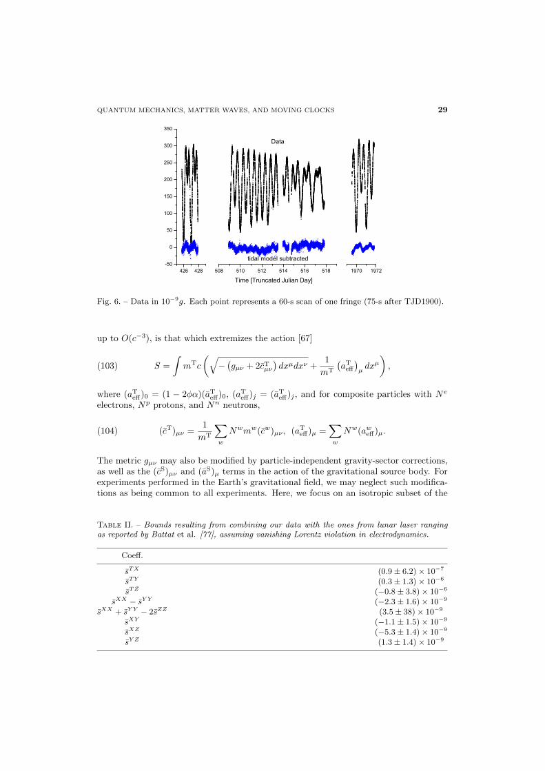
3.2.2. Data analysis and results. Fig. 6 shows the data. It spans about 1500 d, but
is fragmented into three short segments. Major systematic effects in this experimentare tidal variations of the local gravitational acceleration. Subtraction of a Newtonianmodel [75] and an additional model of the local tides [76] yields the residues shown atthe bottom of Fig. 6.
28 HOLGER MULLER
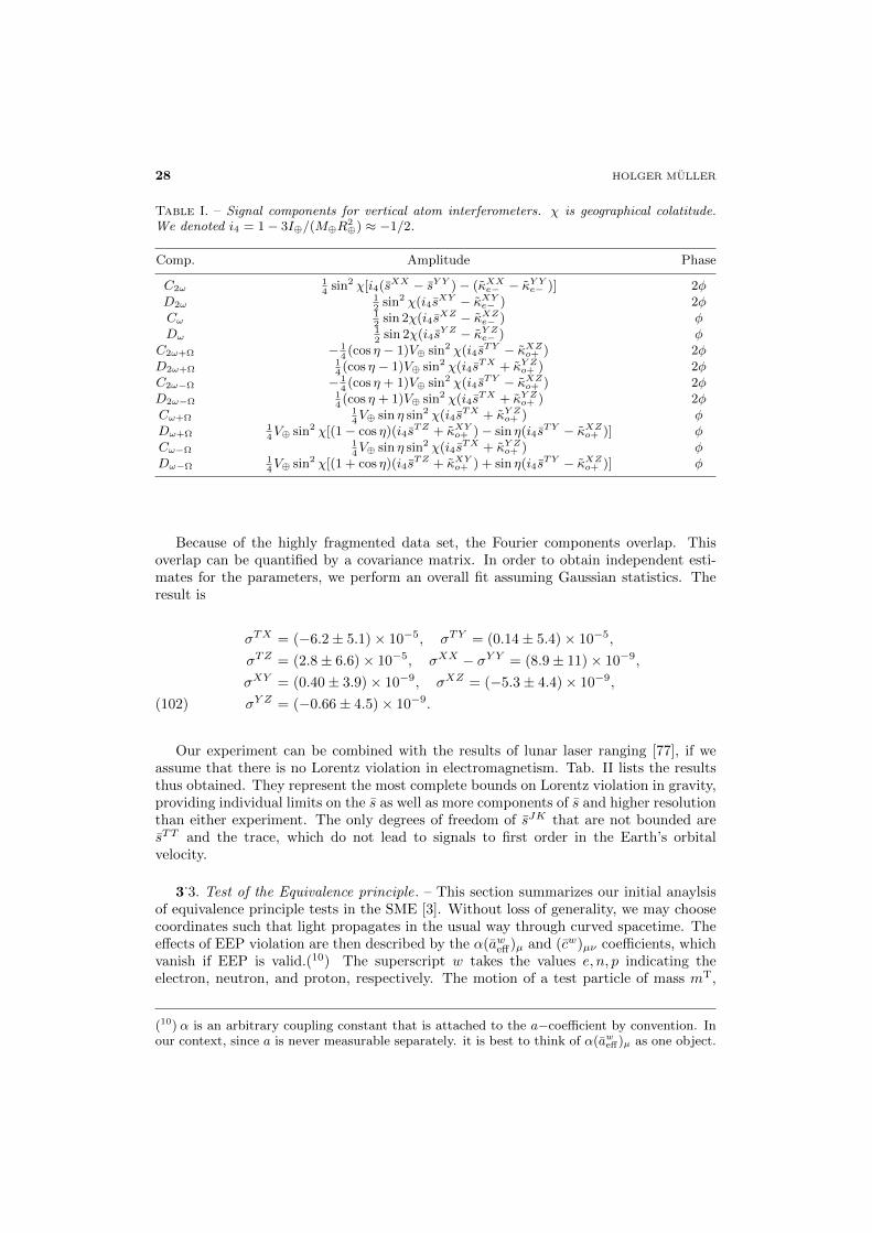
Table I. – Signal components for vertical atom interferometers. χ is geographical colatitude.We denoted i4 = 1− 3I⊕/(M⊕R
2⊕) ≈ −1/2.
Comp. Amplitude Phase
C2ω14
sin2 χ[i4(sXX − sY Y )− (κXXe− − κY Ye− )] 2φD2ω
12
sin2 χ(i4sXY − κXYe− ) 2φ
Cω12
sin 2χ(i4sXZ − κXZe− ) φ
Dω12
sin 2χ(i4sY Z − κY Ze− ) φ
C2ω+Ω − 14(cos η − 1)V⊕ sin2 χ(i4s
TY − κXZo+ ) 2φD2ω+Ω
14(cos η − 1)V⊕ sin2 χ(i4s
TX + κY Zo+ ) 2φC2ω−Ω − 1
4(cos η + 1)V⊕ sin2 χ(i4s
TY − κXZo+ ) 2φD2ω−Ω
14(cos η + 1)V⊕ sin2 χ(i4s
TX + κY Zo+ ) 2φCω+Ω
14V⊕ sin η sin2 χ(i4s
TX + κY Zo+ ) φDω+Ω
14V⊕ sin2 χ[(1− cos η)(i4s
TZ + κXYo+ )− sin η(i4sTY − κXZo+ )] φ
Cω−Ω14V⊕ sin η sin2 χ(i4s
TX + κY Zo+ ) φDω−Ω
14V⊕ sin2 χ[(1 + cos η)(i4s
TZ + κXYo+ ) + sin η(i4sTY − κXZo+ )] φ
Because of the highly fragmented data set, the Fourier components overlap. Thisoverlap can be quantified by a covariance matrix. In order to obtain independent esti-mates for the parameters, we perform an overall fit assuming Gaussian statistics. Theresult is
σTX = (−6.2± 5.1)× 10−5, σTY = (0.14± 5.4)× 10−5,
σTZ = (2.8± 6.6)× 10−5, σXX − σY Y = (8.9± 11)× 10−9,
σXY = (0.40± 3.9)× 10−9, σXZ = (−5.3± 4.4)× 10−9,
σY Z = (−0.66± 4.5)× 10−9.(102)
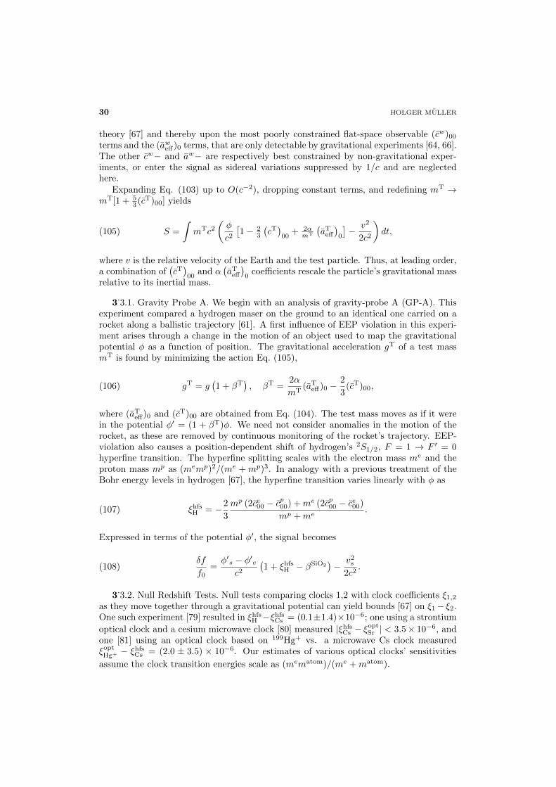
Our experiment can be combined with the results of lunar laser ranging [77], if weassume that there is no Lorentz violation in electromagnetism. Tab. II lists the resultsthus obtained. They represent the most complete bounds on Lorentz violation in gravity,providing individual limits on the s as well as more components of s and higher resolutionthan either experiment. The only degrees of freedom of sJK that are not bounded aresTT and the trace, which do not lead to signals to first order in the Earth’s orbitalvelocity.
3.3. Test of the Equivalence principle. – This section summarizes our initial anaylsis
of equivalence principle tests in the SME [3]. Without loss of generality, we may choosecoordinates such that light propagates in the usual way through curved spacetime. Theeffects of EEP violation are then described by the α(aweff)µ and (cw)µν coefficients, whichvanish if EEP is valid.(10) The superscript w takes the values e, n, p indicating theelectron, neutron, and proton, respectively. The motion of a test particle of mass mT,
(10) α is an arbitrary coupling constant that is attached to the a−coefficient by convention. Inour context, since a is never measurable separately. it is best to think of α(aweff)µ as one object.
QUANTUM MECHANICS, MATTER WAVES, AND MOVING CLOCKS 29
Fig. 6. – Data in 10−9g. Each point represents a 60-s scan of one fringe (75-s after TJD1900).
up to O(c−3), is that which extremizes the action [67]
(103) S =
∫mTc
(√−(gµν + 2cTµν
)dxµdxν +
1
mT
(aT
eff
)µdxµ
),
where (aTeff)0 = (1 − 2φα)(aT
eff)0, (aTeff)j = (aT
eff)j , and for composite particles with Ne
electrons, Np protons, and Nn neutrons,
(104) (cT)µν =1
mT
∑w
Nwmw(cw)µν , (aTeff)µ =
∑w
Nw(aweff)µ.
The metric gµν may also be modified by particle-independent gravity-sector corrections,as well as the (cS)µν and (aS)µ terms in the action of the gravitational source body. Forexperiments performed in the Earth’s gravitational field, we may neglect such modifica-tions as being common to all experiments. Here, we focus on an isotropic subset of the
Table II. – Bounds resulting from combining our data with the ones from lunar laser rangingas reported by Battat et al. [77], assuming vanishing Lorentz violation in electrodynamics.
Coeff.
sTX (0.9± 6.2)× 10−7
sTY (0.3± 1.3)× 10−6
sTZ (−0.8± 3.8)× 10−6
sXX − sY Y (−2.3± 1.6)× 10−9
sXX + sY Y − 2sZZ (3.5± 38)× 10−9
sXY (−1.1± 1.5)× 10−9
sXZ (−5.3± 1.4)× 10−9
sY Z (1.3± 1.4)× 10−9
30 HOLGER MULLER
theory [67] and thereby upon the most poorly constrained flat-space observable (cw)00
terms and the (aweff)0 terms, that are only detectable by gravitational experiments [64, 66].The other cw− and aw− are respectively best constrained by non-gravitational exper-iments, or enter the signal as sidereal variations suppressed by 1/c and are neglectedhere.
Expanding Eq. (103) up to O(c−2), dropping constant terms, and redefining mT →mT[1 + 5
3 (cT)00] yields
(105) S =
∫mTc2
(φ
c2[1− 2
3
(cT)
00+ 2α
mT
(aT
eff
)0
]− v2
2c2
)dt,
where v is the relative velocity of the Earth and the test particle. Thus, at leading order,a combination of
(cT)
00and α
(aT
eff
)0
coefficients rescale the particle’s gravitational massrelative to its inertial mass.
3.3.1. Gravity Probe A. We begin with an analysis of gravity-probe A (GP-A). This
experiment compared a hydrogen maser on the ground to an identical one carried on arocket along a ballistic trajectory [61]. A first influence of EEP violation in this experi-ment arises through a change in the motion of an object used to map the gravitationalpotential φ as a function of position. The gravitational acceleration gT of a test massmT is found by minimizing the action Eq. (105),
(106) gT = g(1 + βT
), βT =
2α
mT(aT
eff)0 −2
3(cT)00,
where (aTeff)0 and (cT)00 are obtained from Eq. (104). The test mass moves as if it were
in the potential φ′ = (1 + βT)φ. We need not consider anomalies in the motion of therocket, as these are removed by continuous monitoring of the rocket’s trajectory. EEP-violation also causes a position-dependent shift of hydrogen’s 2S1/2, F = 1 → F ′ = 0hyperfine transition. The hyperfine splitting scales with the electron mass me and theproton mass mp as (memp)2/(me + mp)3. In analogy with a previous treatment of theBohr energy levels in hydrogen [67], the hyperfine transition varies linearly with φ as
(107) ξhfsH = −2
3
mp (2ce00 − cp00) +me (2cp00 − ce00)
mp +me.
Expressed in terms of the potential φ′, the signal becomes
(108)δf
f0=φ′s − φ′e
c2(1 + ξhfs
H − βSiO2)− v2
s
2c2.
3.3.2. Null Redshift Tests. Null tests comparing clocks 1,2 with clock coefficients ξ1,2
as they move together through a gravitational potential can yield bounds [67] on ξ1− ξ2.One such experiment [79] resulted in ξhfs
H −ξhfsCs = (0.1±1.4)×10−6; one using a strontium
optical clock and a cesium microwave clock [80] measured |ξhfsCs − ξopt
Sr | < 3.5× 10⁻⁶, andone [81] using an optical clock based on 199Hg+ vs. a microwave Cs clock measuredξoptHg+ − ξhfs
Cs = (2.0 ± 3.5) × 10−6. Our estimates of various optical clocks’ sensitivities
assume the clock transition energies scale as (mematom)/(me +matom).
QUANTUM MECHANICS, MATTER WAVES, AND MOVING CLOCKS 31
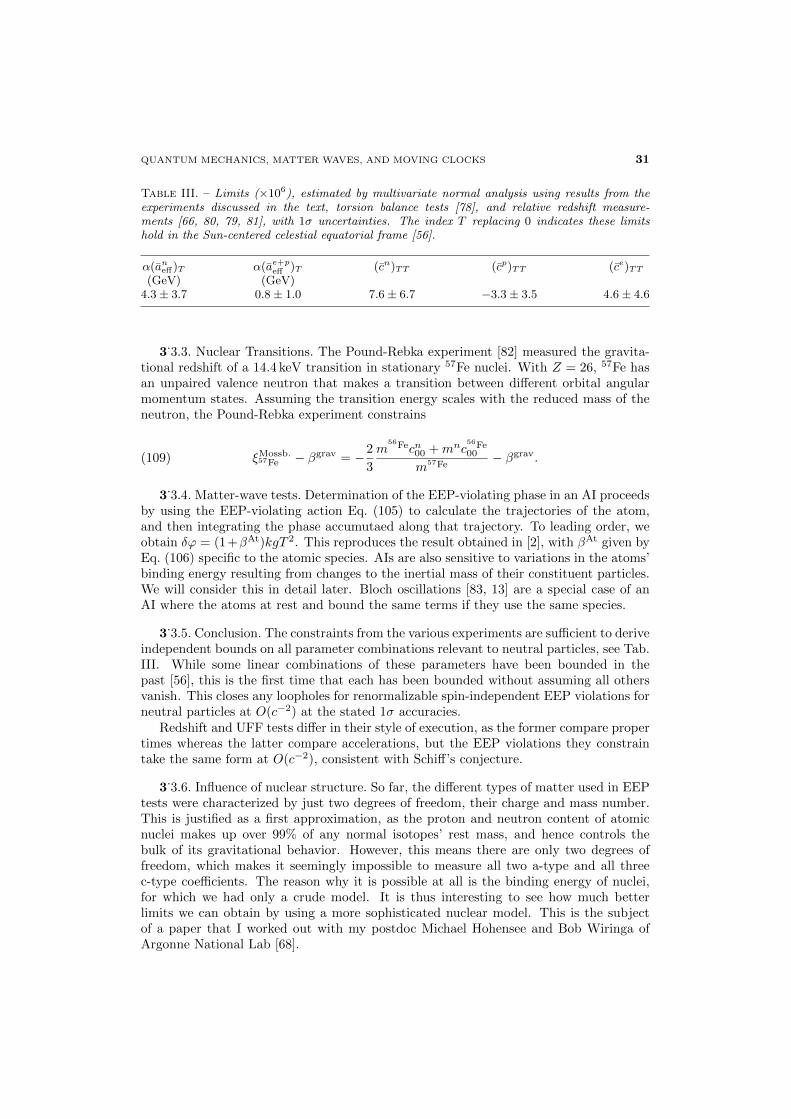
Table III. – Limits (×106), estimated by multivariate normal analysis using results from theexperiments discussed in the text, torsion balance tests [78], and relative redshift measure-ments [66, 80, 79, 81], with 1σ uncertainties. The index T replacing 0 indicates these limitshold in the Sun-centered celestial equatorial frame [56].
α(aneff)T α(ae+peff )T (cn)TT (cp)TT (ce)TT(GeV) (GeV)
4.3± 3.7 0.8± 1.0 7.6± 6.7 −3.3± 3.5 4.6± 4.6
3.3.3. Nuclear Transitions. The Pound-Rebka experiment [82] measured the gravita-
tional redshift of a 14.4 keV transition in stationary 57Fe nuclei. With Z = 26, 57Fe hasan unpaired valence neutron that makes a transition between different orbital angularmomentum states. Assuming the transition energy scales with the reduced mass of theneutron, the Pound-Rebka experiment constrains
(109) ξMossb.57Fe − βgrav = −2
3
m56Fecn00 +mnc
56Fe00
m57Fe− βgrav.
3.3.4. Matter-wave tests. Determination of the EEP-violating phase in an AI proceeds
by using the EEP-violating action Eq. (105) to calculate the trajectories of the atom,and then integrating the phase accumutaed along that trajectory. To leading order, weobtain δϕ = (1+βAt)kgT 2. This reproduces the result obtained in [2], with βAt given byEq. (106) specific to the atomic species. AIs are also sensitive to variations in the atoms’binding energy resulting from changes to the inertial mass of their constituent particles.We will consider this in detail later. Bloch oscillations [83, 13] are a special case of anAI where the atoms at rest and bound the same terms if they use the same species.
3.3.5. Conclusion. The constraints from the various experiments are sufficient to derive
independent bounds on all parameter combinations relevant to neutral particles, see Tab.III. While some linear combinations of these parameters have been bounded in thepast [56], this is the first time that each has been bounded without assuming all othersvanish. This closes any loopholes for renormalizable spin-independent EEP violations forneutral particles at O(c−2) at the stated 1σ accuracies.
Redshift and UFF tests differ in their style of execution, as the former compare propertimes whereas the latter compare accelerations, but the EEP violations they constraintake the same form at O(c−2), consistent with Schiff’s conjecture.
3.3.6. Influence of nuclear structure. So far, the different types of matter used in EEP
tests were characterized by just two degrees of freedom, their charge and mass number.This is justified as a first approximation, as the proton and neutron content of atomicnuclei makes up over 99% of any normal isotopes’ rest mass, and hence controls thebulk of its gravitational behavior. However, this means there are only two degrees offreedom, which makes it seemingly impossible to measure all two a-type and all threec-type coefficients. The reason why it is possible at all is the binding energy of nuclei,for which we had only a crude model. It is thus interesting to see how much betterlimits we can obtain by using a more sophisticated nuclear model. This is the subjectof a paper that I worked out with my postdoc Michael Hohensee and Bob Wiringa ofArgonne National Lab [68].
32 HOLGER MULLER
Using a nuclear shell model, we estimate the sensitivity of a variety of atomic nucleito EEP violation for matter and antimatter. We also illustrate points of commonalitybetween older representations of EEP violation based on neutron excess and baryonnumber, and that of the SME. Existing experimental [84, 2, 85, 61, 82, 88, 79, 80, 81, 87]limits on spin-independent EEP violation in matter and antimatter [3] yield limits onSME coefficients that are significantly tighter than previously thought. As before, weassume that anomalies affecting force-carrying virtual particles are negligible. We defineour coordinates such that photons follow null geodesics, ensuring that electromagneticfields do not violate EEP.
For a bound system of particles, the total Hamiltonian is a sum of single-particleHamiltonians, plus an interaction energy Vint that is assumed to be free of EEP-violatingterms. For a freely falling nucleus, e.g., the kinetic energy of the center of mass motion(with velocity v2) is small compared to the rest mass-energy. It is of similar order asthe relevant change ∆U it explores in the gravitational potential. Since its protons andneutrons are non-gravitationally bound, however, we cannot assume that the same is truefor the kinetic energy of its constituent particles, which are in fact at the percent-levelof the rest mass. Thus, we include terms proportional to v2
w,jU/c2 in our Hamiltonian,
where vw,j is the instantaneous velocity of the jth bound particle of species w.For any particular EEP test comparing the effects of gravity acting on systems A and
B, the observable anomaly is given by βA − βB , where βA and βB are the sensitivitycoefficients of the two systems. Since all high-precision tests of EEP are performedon charge-neutral systems, and since normal matter has a substantially similar ratio ofproton to neutron content, the expression for βA−βB can be usefully expressed in termsof an effective neutron excess ∆j and effective mass defect m′j
∆j ≡mn
mp
me +mp
mnNnj −Np
j ,(110)
m′j ≡ m′j −(mn −mp)(me +mp)
mnNpj ,(111)
where j ∈ A,B. The EEP-violating observable can then be written in terms of linearcombinations of the free particle (βw) and anti-particle (βw) anomalies as
βA − βB =(mn)2
(mn)2 + (me +mp)2
[(∆A
MA− ∆B
MB
)(∆A
MA− ∆B
MB
)mpβe+p−n
−(m′AMA− m′BMB
)βe+p+n
]− 1
2
∑w
(TwA,int
MAc2−TwB,int
MBc2
)(βw + βw
),(112)
where TwB,int are the bound kinetic energies of the particles, MA and MB are the massesof the two test bodies, and(113)
βe+p−n ≡ βe+p − me +mp
mnβn, βe+p+n ≡ me +mp
mnβe+p + βn, βe+p ≡ me
mpβe + βp,
similar to definitions used in [86]. We can define a similar set of terms βe+p, βe+p−n,and βe+p+n for antimatter. Thus the quantities mpβe+p−n and mnβe+p+n in the SMEmay be understood as parameterizing an anomalous gravitational coupling to a givenparticle’s neutron-excess and total baryon number “charges” [86].
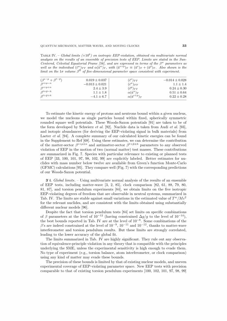
QUANTUM MECHANICS, MATTER WAVES, AND MOVING CLOCKS 33
Table IV. – Global limits (×106) on isotropic EEP-violation, obtained via multivariate normalanalysis on the results of an ensemble of precision tests of EEP. Limits are stated in the Sun-Centered, Celestial Equatorial Frame [56], and are expressed in terms of the βw parameters aswell as the individual (cw)TT and α(aw)T , with (ae+p)T ≡ (ae)T + (ap)T . Also shown is thelimit on the 1σ volume βΠ of five-dimensional parameter space consistent with experiment.
(βe−p + βe−p) 0.019± 0.037 (ce)TT −0.014± 0.028βe+p−n −0.013± 0.021 (cn)TT 1.1± 1.4βe+p+n 2.4± 3.9 (cp)TT 0.24± 0.30βe+p−n 1.1± 1.8 α(an)T 0.51± 0.64βe+p+n −4.1± 6.7 α(ae+p)T 0.22± 0.28
To estimate the kinetic energy of protons and neutrons bound within a given nucleus,we model the nucleons as single particles bound within fixed, spherically symmetricrounded square well potentials. These Woods-Saxon potentials [91] are taken to be ofthe form developed by Schwierz et al. [92]. Nuclide data is taken from Audi et al. [93],and isotopic abundances (for deriving the EEP-violating signal in bulk materials) fromLaeter et al. [94]. A complete summary of our calculated kinetic energies can be foundin the Supplement to Ref [68]. Using these estimates, we can determine the contributionof the matter-sector βe+p±n and antimatter-sector βe+p±n parameters to any observedviolation of EEP in the motion of two (normal matter) test masses. These contributionsare summarized in Fig. 7. Species with particular relevance to existing or planned testsof EEP [33, 100, 101, 97, 98, 102, 99] are explicitly labeled. Better estimates for nu-clides with mass number below twelve are available from Green’s function Monte-Carlo(GFMC) calculations [95]. They compare well (Fig. 7) with the corresponding predictionsof our Woods-Saxon potential.
3.4. Global limits. – Using multivariate normal analysis of the results of an ensemble
of EEP tests, including matter-wave [3, 2, 85], clock comparison [82, 61, 88, 79, 80,81, 87], and torsion pendulum experiments [84], we obtain limits on the five isotropicEEP-violating degrees of freedom that are observable in neutral systems, summarized inTab. IV. The limits are stable against small variations in the estimated value of Tw/Mc2
for the relevant nuclides, and are consistent with the limits obtained using substantiallydifferent nuclear models [96].
Despite the fact that torsion pendulum tests [84] set limits on specific combinationsof β parameters at the level of 10−12 (having constrained ∆g/g to the level of 10−14),the best bounds reported in Tab. IV are at the level of 10−8. Some combinations of theβ’s are indeed constrained at the level of 10−9, 10−11 and 10−12, thanks to matter-waveinterferometer and torsion pendulum results. But these limits are strongly correlated,leading to the lower accuracy of the global fit.
The limits summarized in Tab. IV are highly significant. They rule out any observa-tion of equivalence-principle violation in any theory that is compatible with the principlesunderlying the SME, unless the experimental sensitivity is high enough to evade them.No type of experiment (e.g., torsion balance, atom interferometer, or clock comparison)using any kind of matter may evade these bounds.
The precision of these bounds is limited by that of existing nuclear models, and unevenexperimental coverage of EEP-violating parameter space. New EEP tests with precisioncomparable to that of existing torsion pendulum experiments [100, 102, 101, 97, 98, 99]
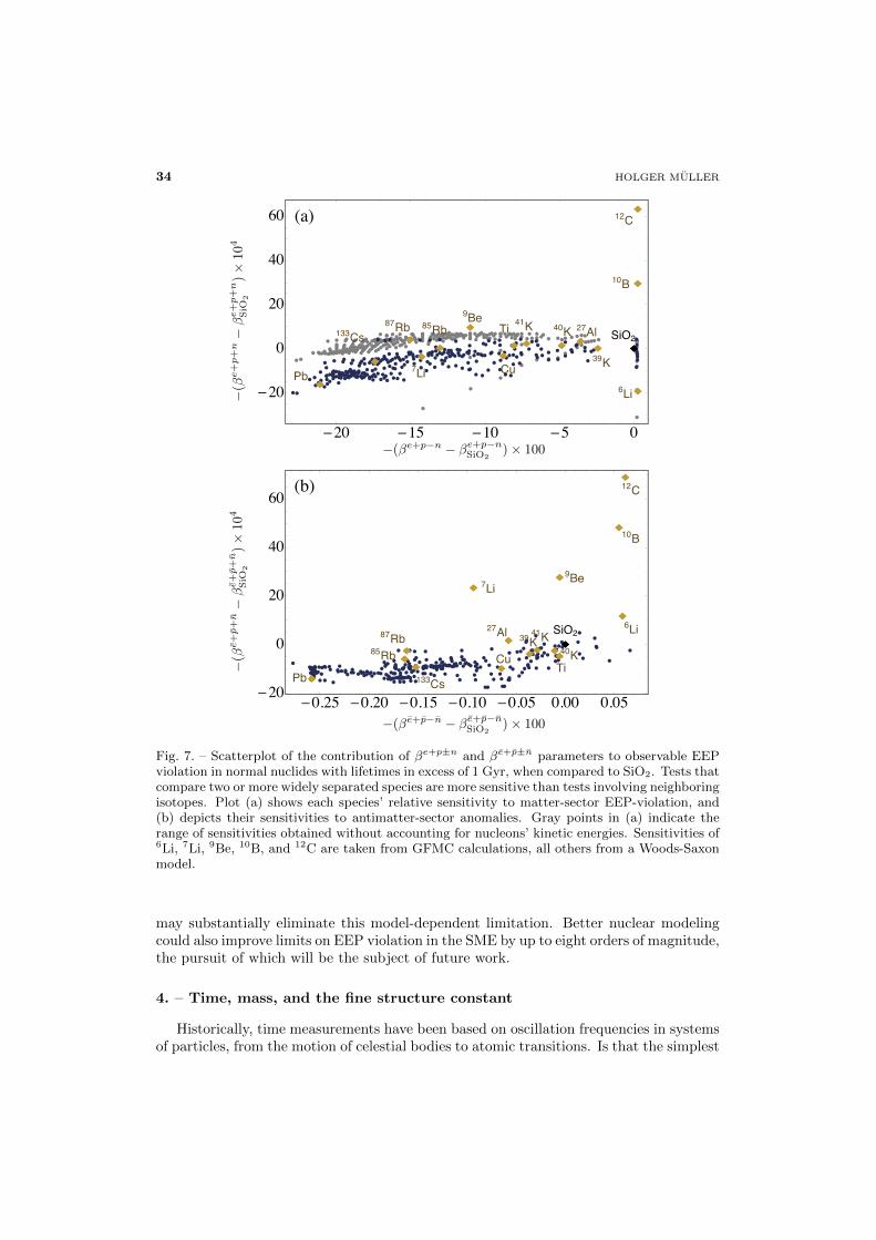
34 HOLGER MULLER
87Rb
85Rb
6Li
7Li
10B
12C
39K40K
41K27Al
133Cs
9Be
SiO2
Ti
Cu
Pb
0.25 0.20 0.15 0.10 0.05 0.00 0.0520
0
20
40
60
−(βe+p−n − βe+p−nSiO2
)× 100
−(β
e+p+n−
βe+p+n
SiO
2)×
104
−(β
e+p+n−βe+p+n
SiO
2)×
104
−(βe+p−n − βe+p−nSiO2
)× 100
(a)
(b)
87Rb
85Rb
6Li
7Li
10B
12C
39K
40K
41K27Al
133Cs9Be
SiO2
Ti
Cu
Pb
20 15 10 5 0
20
0
20
40
60
Fig. 7. – Scatterplot of the contribution of βe+p±n and βe+p±n parameters to observable EEPviolation in normal nuclides with lifetimes in excess of 1 Gyr, when compared to SiO2. Tests thatcompare two or more widely separated species are more sensitive than tests involving neighboringisotopes. Plot (a) shows each species’ relative sensitivity to matter-sector EEP-violation, and(b) depicts their sensitivities to antimatter-sector anomalies. Gray points in (a) indicate therange of sensitivities obtained without accounting for nucleons’ kinetic energies. Sensitivities of6Li, 7Li, 9Be, 10B, and 12C are taken from GFMC calculations, all others from a Woods-Saxonmodel.
may substantially eliminate this model-dependent limitation. Better nuclear modelingcould also improve limits on EEP violation in the SME by up to eight orders of magnitude,the pursuit of which will be the subject of future work.
4. – Time, mass, and the fine structure constant
Historically, time measurements have been based on oscillation frequencies in systemsof particles, from the motion of celestial bodies to atomic transitions. Is that the simplest
QUANTUM MECHANICS, MATTER WAVES, AND MOVING CLOCKS 35
possible clock, i.e., is it impossible to measure time in absence of multi-particle systems?Relativity and quantum mechanics show that even a single particle of mass m determinesa Compton frequency ωC = mc2/~. A clock referenced to the Compton frequency wouldenable high-precision mass measurements and a fundamental definition of the second.We demonstrate such a Compton clock using an optical frequency comb to self-referencea Ramsey-Borde atom interferometer and synchronize an oscillator at a subharmonic ofωC [26]. This directly demonstrates the connection between time and mass. It allowsmeasurement of microscopic masses with 4× 10⁻⁹ accuracy in the proposed revision toSI units. Together with the Avogadro project, it yields calibrated kilograms. MeasuringωC is equivalent to measuring h/m. From ωC or h/m, the fine structure constant canbe calculated and thus be measured by atom interferometry [27]. Since the topics ofmeasuring time, mass, and the fine structure constant with atom interferometry are thusclosely related, we describe them together in this chapter.
4.1. Our atomic-fountain interferometer . – Atoms are assembled in a two-dimensional
magneto-optical trap (2D-MOT), loaded into a 3D-MOT and launched vertically upwardswith a moving molasses. A sample having a measured 3-D temperature of 1.2µK islaunched vertically to a height of 1-m in ultra-high vacuum every 2.1 seconds. Furtherpreparation stages select a subset of atoms that have a narrow velocity distributionin the vertical direction corresponding to a temperature of 5.5 nK and that are in theF = 3,mF = 0 quantum state, which is magnetic-field insensitive to the leading order.We perform interferometry with ∼ 106 atoms during the ∼1-s of free fall.
The free fall of the atoms causes a Doppler shift which we compensate for by rampingthe laser frequency difference at a rate of r = gωL/c ≈ 11.5 MHz/s in the laser’s restframe. The ramp (provided by an Analog Devices AD9954 synthesizer) has a step size of∼ 0.01µs, i.e., is essentially smooth even on the time-scale of a single Bragg pulse. Forfluorescence detection, the atoms are excited on the F = 4,mF = 4 → F ′ = 5,mF ′ = 5cycling transition and their fluorescence is detected using a Hamamatsu R943-02 photo-multiplier tube.
4.1.1. Bragg diffraction. In multiphoton Bragg diffraction, the atom coherently scat-
ters 2n photons from a pair of antiparallel laser beams, without changing its internalstate. The atom thereby acquires a kinetic energy of 4n2~ωr, where ωr = ~k2/(2M) isthe recoil frequency and M the mass of the atom. Matching with the energy n~(ω1−ω2)lost by the laser field defines the resonance condition for the difference frequency ω1−ω2
of the beams.Bragg diffraction helps increase the signal, which scales quadratically with momentum
transfer in recoil measurements, and is thus our method of choice. It also helps suppressthe sensitivity to magnetic fields, as the atoms are in the same internal state in bothinterferometer arms. Fig. 8 shows interference fringes measured with various degrees ofhigh-order Bragg diffraction [106].
4.2. Simultaneous interferometers. – To make the Compton clock and recoil measure-
ments independent of g or the ramp rate r, we simultaneously operate a pair of conjugateinterferometers, with the direction of the recoil reversed relative to each other. This alsocancels accelerations from vibrations and is now a routine method, described in [143].
4.2.1. Laser system. High-powered laser beams are mandatory for driving high-order
multiphoton Bragg diffraction: The effective Rabi frequency [105] Ωeff ≈ Ωn/[(8ωr)n−1(n−
1)!2] is a very strong function of the 2-photon Rabi frequency Ω, and beams of large radius
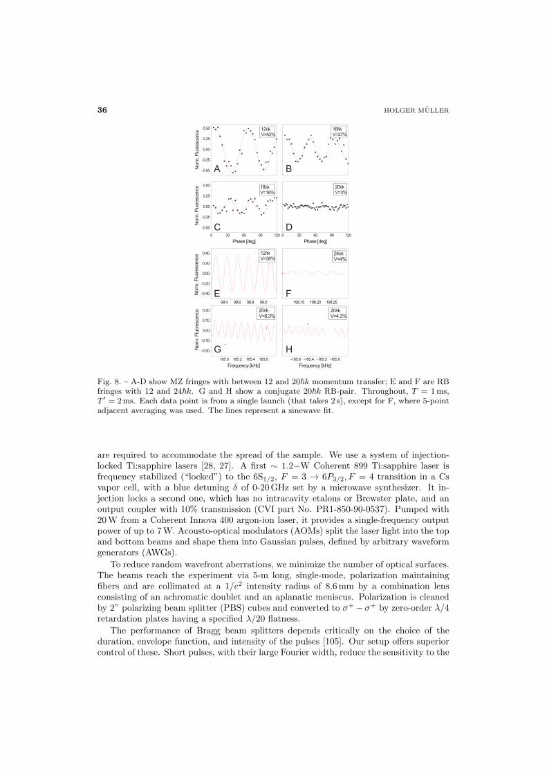
36 HOLGER MULLER
-0.50
-0.25
0.00
0.25
0.50 12kV=52%
Norm
.Flu
ore
scence
16kV=27%
0 30 60 90 120
-0.50
-0.25
0.00
0.25
0.50 18kV=16%
Norm
.Flu
ore
scence
Phase [deg]
0 30 60 90 120
20kV=3%
Phase [deg]
98.4 98.6 98.8 99.0
-0.40
-0.20
0.00
0.20
0.40 12kV=36%
Norm
.Flu
ore
scence
198.15 198.20 198.25
24kV=4%
165.0 165.2 165.4 165.6
-0.20
-0.10
0.00
0.10
0.20 20kV=8.3%
Norm
.Flu
ore
scence
Frequency [kHz]
-165.6 -165.4 -165.2 -165.0
20kV=4.3%
Frequency [kHz]
A B
C D
E F
G H
Fig. 8. – A-D show MZ fringes with between 12 and 20~k momentum transfer; E and F are RBfringes with 12 and 24~k. G and H show a conjugate 20~k RB-pair. Throughout, T = 1 ms,T ′ = 2 ms. Each data point is from a single launch (that takes 2 s), except for F, where 5-pointadjacent averaging was used. The lines represent a sinewave fit.
are required to accommodate the spread of the sample. We use a system of injection-locked Ti:sapphire lasers [28, 27]. A first ∼ 1.2−W Coherent 899 Ti:sapphire laser isfrequency stabilized (“locked”) to the 6S1/2, F = 3 → 6P3/2, F = 4 transition in a Csvapor cell, with a blue detuning δ of 0-20 GHz set by a microwave synthesizer. It in-jection locks a second one, which has no intracavity etalons or Brewster plate, and anoutput coupler with 10% transmission (CVI part No. PR1-850-90-0537). Pumped with20 W from a Coherent Innova 400 argon-ion laser, it provides a single-frequency outputpower of up to 7 W. Acousto-optical modulators (AOMs) split the laser light into the topand bottom beams and shape them into Gaussian pulses, defined by arbitrary waveformgenerators (AWGs).
To reduce random wavefront aberrations, we minimize the number of optical surfaces.The beams reach the experiment via 5-m long, single-mode, polarization maintainingfibers and are collimated at a 1/e2 intensity radius of 8.6 mm by a combination lensconsisting of an achromatic doublet and an aplanatic meniscus. Polarization is cleanedby 2” polarizing beam splitter (PBS) cubes and converted to σ+− σ+ by zero-order λ/4retardation plates having a specified λ/20 flatness.
The performance of Bragg beam splitters depends critically on the choice of theduration, envelope function, and intensity of the pulses [105]. Our setup offers superiorcontrol of these. Short pulses, with their large Fourier width, reduce the sensitivity to the
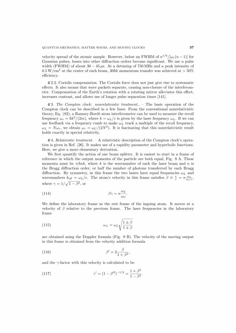
QUANTUM MECHANICS, MATTER WAVES, AND MOVING CLOCKS 37
velocity spread of the atomic sample. However, below an FWHM of n1/6/[ωr(n− 1)] forGaussian pulses, losses into other diffraction orders become significant. We use a pulsewidth (FWHM) of about 30− 45µs. At a detuning of 750 MHz and a peak intensity of0.5 W/cm2 at the center of each beam, 30~k momentum transfer was achieved at > 50%efficiency.
4.2.2. Coriolis compensation. The Coriolis force does not just give rise to systematic
effects. It also means that wave packets separate, causing non-closure of the interferom-eter. Compensation of the Earth’s rotation with a rotating mirror alleviates this effect,increases contrast, and allows use of longer pulse separation times [141].
4.3. The Compton clock: nonrelativistic treatment.. – The basic operation of the
Compton clock can be described in a few lines: From the conventional nonrelativistictheory, Eq. (82), a Ramsey-Borde atom interferometer can be used to measure the recoilfrequency ωr = ~k2/(2m), where k = ωL/c is given by the laser frequency ωL. If we canuse feedback via a frequency comb to make ωL track a multiple of the recoil frequency,ωL = Nωr, we obtain ωr = ωC/(2N
2). It is fascinating that this nonrelativistic resultholds exactly in special relativity.
4.4. Relativistic treatment . – A relativistic description of the Compton clock’s opera-
tion is given in Ref. [26]. It makes use of a rapidity parameter and hyperbolic functions.Here, we give a more elementary derivation.
We first quantify the action of one beam splitter. It is easiest to start in a frame ofreference in which the output momenta of the particle are both equal, Fig. 9 A. Thesemomenta must be ±~nk, where k is the wavenumber of each the laser beam and n isthe Bragg diffraction order, or half the number of photons transferred by each Braggdiffraction. By symmetry, in this frame the two lasers have equal frequencies ωL andwavenumbers keff = ωL/c. The atom’s velocity in this frame satisfies β ≡ v
c = n ωLωCγ
,
where γ = 1/√
1− β2, or
(114) βγ = nωLωC
.
We define the laboratory frame as the rest frame of the ingoing atom. It moves at avelocity of β relative to the previous frame. The laser frequencies in the laboratoryframe
(115) ω± = ωL
√1± β1∓ β
are obtained using the Doppler formula (Fig. 9 B). The velocity of the moving outputin this frame is obtained from the velocity addition formula
(116) β′ = 2β
1 + β2,
and the γ-factor with this velocity is calculated to be
(117) γ′ = (1− β′2)−1/2 =1 + β2
1− β2.
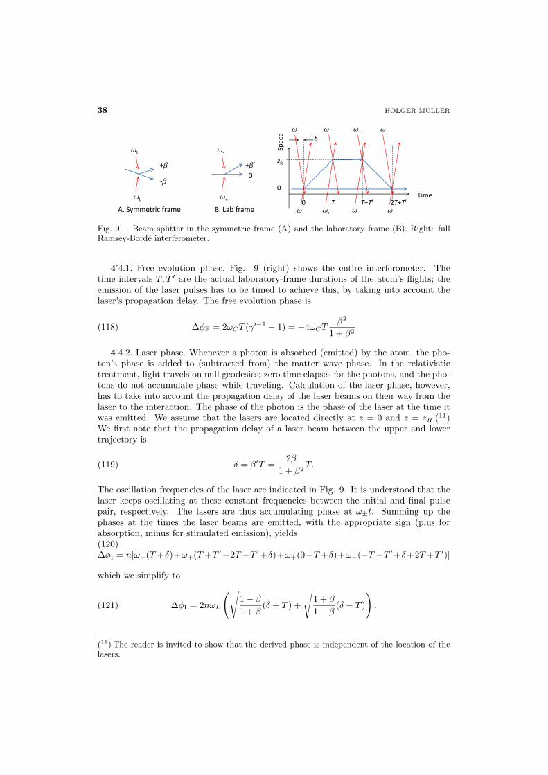
38 HOLGER MULLER
L
L
+
-
A. Symmetric frame
0
B. Lab frame
-
+
+’
δ
0 T T+T’ 2T+T’ Time
Spac
e
zR
0
- - + +
+ + - -
Fig. 9. – Beam splitter in the symmetric frame (A) and the laboratory frame (B). Right: fullRamsey-Borde interferometer.
4.4.1. Free evolution phase. Fig. 9 (right) shows the entire interferometer. The
time intervals T, T ′ are the actual laboratory-frame durations of the atom’s flights; theemission of the laser pulses has to be timed to achieve this, by taking into account thelaser’s propagation delay. The free evolution phase is
(118) ∆φF = 2ωCT (γ′−1 − 1) = −4ωCTβ2
1 + β2
4.4.2. Laser phase. Whenever a photon is absorbed (emitted) by the atom, the pho-
ton’s phase is added to (subtracted from) the matter wave phase. In the relativistictreatment, light travels on null geodesics; zero time elapses for the photons, and the pho-tons do not accumulate phase while traveling. Calculation of the laser phase, however,has to take into account the propagation delay of the laser beams on their way from thelaser to the interaction. The phase of the photon is the phase of the laser at the time itwas emitted. We assume that the lasers are located directly at z = 0 and z = zR.(11)We first note that the propagation delay of a laser beam between the upper and lowertrajectory is
(119) δ = β′T =2β
1 + β2T.
The oscillation frequencies of the laser are indicated in Fig. 9. It is understood that thelaser keeps oscillating at these constant frequencies between the initial and final pulsepair, respectively. The lasers are thus accumulating phase at ω±t. Summing up thephases at the times the laser beams are emitted, with the appropriate sign (plus forabsorption, minus for stimulated emission), yields(120)∆φI = n[ω−(T+δ)+ω+(T+T ′−2T−T ′+δ)+ω+(0−T+δ)+ω−(−T−T ′+δ+2T+T ′)]
which we simplify to
(121) ∆φI = 2nωL
(√1− β1 + β
(δ + T ) +
√1 + β
1− β (δ − T )
).
(11) The reader is invited to show that the derived phase is independent of the location of thelasers.
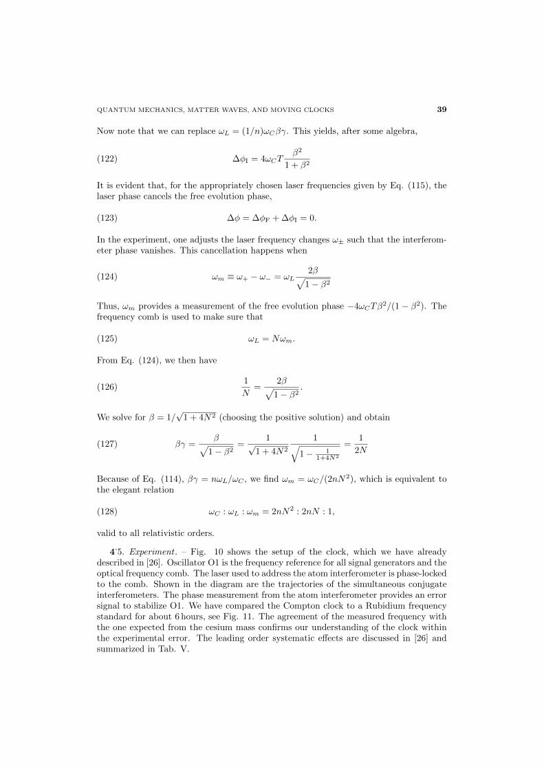
QUANTUM MECHANICS, MATTER WAVES, AND MOVING CLOCKS 39
Now note that we can replace ωL = (1/n)ωCβγ. This yields, after some algebra,
(122) ∆φI = 4ωCTβ2
1 + β2
It is evident that, for the appropriately chosen laser frequencies given by Eq. (115), thelaser phase cancels the free evolution phase,
(123) ∆φ = ∆φF + ∆φI = 0.
In the experiment, one adjusts the laser frequency changes ω± such that the interferom-eter phase vanishes. This cancellation happens when
(124) ωm ≡ ω+ − ω− = ωL2β√
1− β2
Thus, ωm provides a measurement of the free evolution phase −4ωCTβ2/(1− β2). The
frequency comb is used to make sure that
(125) ωL = Nωm.
From Eq. (124), we then have
(126)1
N=
2β√1− β2
.
We solve for β = 1/√
1 + 4N2 (choosing the positive solution) and obtain
(127) βγ =β√
1− β2=
1√1 + 4N2
1√1− 1
1+4N2
=1
2N
Because of Eq. (114), βγ = nωL/ωC , we find ωm = ωC/(2nN2), which is equivalent to
the elegant relation
(128) ωC : ωL : ωm = 2nN2 : 2nN : 1,
valid to all relativistic orders.
4.5. Experiment . – Fig. 10 shows the setup of the clock, which we have already
described in [26]. Oscillator O1 is the frequency reference for all signal generators and theoptical frequency comb. The laser used to address the atom interferometer is phase-lockedto the comb. Shown in the diagram are the trajectories of the simultaneous conjugateinterferometers. The phase measurement from the atom interferometer provides an errorsignal to stabilize O1. We have compared the Compton clock to a Rubidium frequencystandard for about 6 hours, see Fig. 11. The agreement of the measured frequency withthe one expected from the cesium mass confirms our understanding of the clock withinthe experimental error. The leading order systematic effects are discussed in [26] andsummarized in Tab. V.
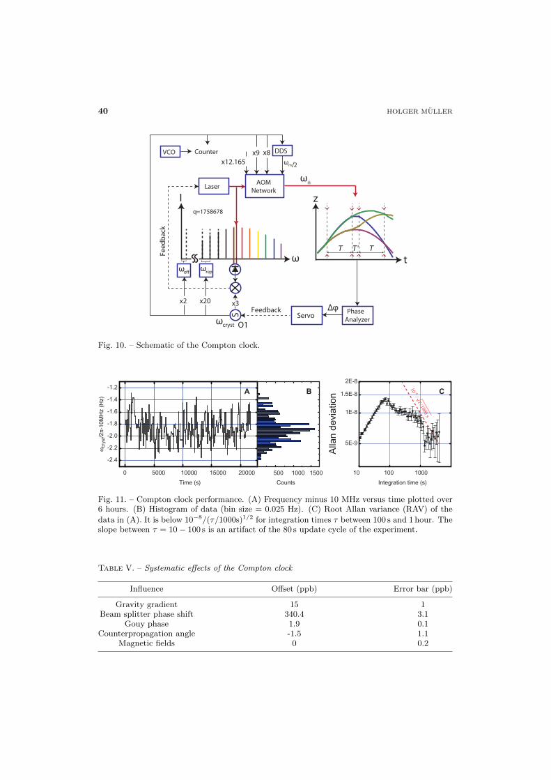
40 HOLGER MULLER
Fig. 10. – Schematic of the Compton clock.
Fig. 11. – Compton clock performance. (A) Frequency minus 10 MHz versus time plotted over6 hours. (B) Histogram of data (bin size = 0.025 Hz). (C) Root Allan variance (RAV) of the
data in (A). It is below 10−8/(τ/1000s)1/2 for integration times τ between 100 s and 1 hour. Theslope between τ = 10− 100 s is an artifact of the 80 s update cycle of the experiment.
Table V. – Systematic effects of the Compton clock
Influence Offset (ppb) Error bar (ppb)
Gravity gradient 15 1Beam splitter phase shift 340.4 3.1
Gouy phase 1.9 0.1Counterpropagation angle -1.5 1.1
Magnetic fields 0 0.2
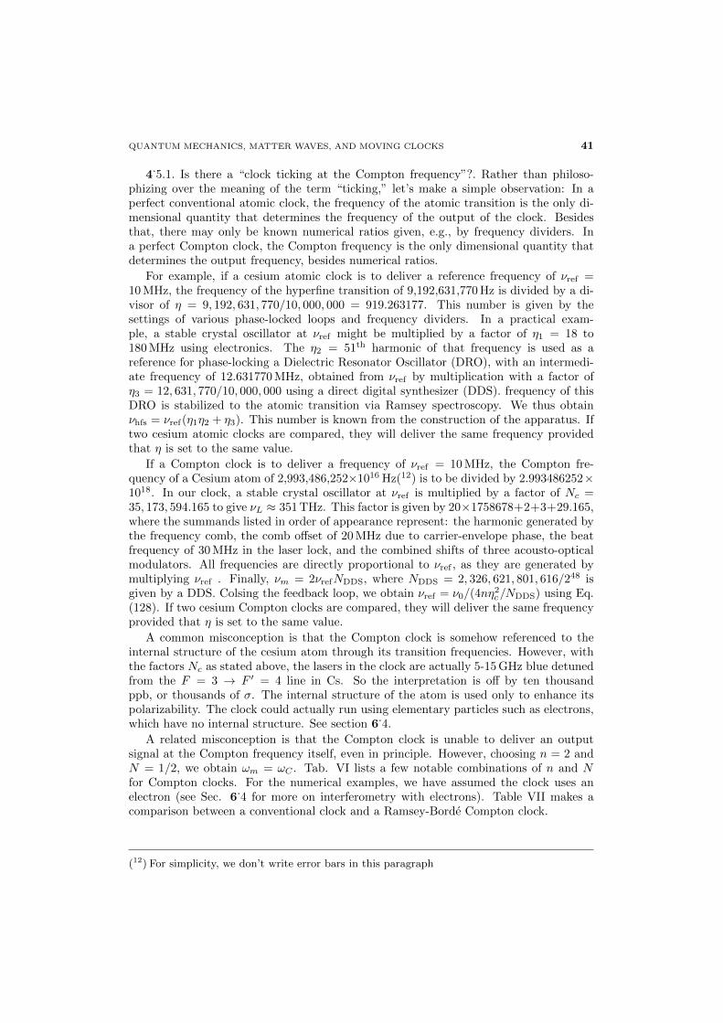
QUANTUM MECHANICS, MATTER WAVES, AND MOVING CLOCKS 41
4.5.1. Is there a “clock ticking at the Compton frequency”?. Rather than philoso-
phizing over the meaning of the term “ticking,” let’s make a simple observation: In aperfect conventional atomic clock, the frequency of the atomic transition is the only di-mensional quantity that determines the frequency of the output of the clock. Besidesthat, there may only be known numerical ratios given, e.g., by frequency dividers. Ina perfect Compton clock, the Compton frequency is the only dimensional quantity thatdetermines the output frequency, besides numerical ratios.
For example, if a cesium atomic clock is to deliver a reference frequency of νref =10 MHz, the frequency of the hyperfine transition of 9,192,631,770 Hz is divided by a di-visor of η = 9, 192, 631, 770/10, 000, 000 = 919.263177. This number is given by thesettings of various phase-locked loops and frequency dividers. In a practical exam-ple, a stable crystal oscillator at νref might be multiplied by a factor of η1 = 18 to180 MHz using electronics. The η2 = 51th harmonic of that frequency is used as areference for phase-locking a Dielectric Resonator Oscillator (DRO), with an intermedi-ate frequency of 12.631770 MHz, obtained from νref by multiplication with a factor ofη3 = 12, 631, 770/10, 000, 000 using a direct digital synthesizer (DDS). frequency of thisDRO is stabilized to the atomic transition via Ramsey spectroscopy. We thus obtainνhfs = νref(η1η2 + η3). This number is known from the construction of the apparatus. Iftwo cesium atomic clocks are compared, they will deliver the same frequency providedthat η is set to the same value.
If a Compton clock is to deliver a frequency of νref = 10 MHz, the Compton fre-quency of a Cesium atom of 2,993,486,252×1016 Hz(12) is to be divided by 2.993486252×10¹⁸. In our clock, a stable crystal oscillator at νref is multiplied by a factor of Nc =35, 173, 594.165 to give νL ≈ 351 THz. This factor is given by 20×1758678+2+3+29.165,where the summands listed in order of appearance represent: the harmonic generated bythe frequency comb, the comb offset of 20 MHz due to carrier-envelope phase, the beatfrequency of 30 MHz in the laser lock, and the combined shifts of three acousto-opticalmodulators. All frequencies are directly proportional to νref , as they are generated bymultiplying νref . Finally, νm = 2νrefNDDS, where NDDS = 2, 326, 621, 801, 616/248 isgiven by a DDS. Colsing the feedback loop, we obtain νref = ν0/(4nη
2c/NDDS) using Eq.
(128). If two cesium Compton clocks are compared, they will deliver the same frequencyprovided that η is set to the same value.
A common misconception is that the Compton clock is somehow referenced to theinternal structure of the cesium atom through its transition frequencies. However, withthe factors Nc as stated above, the lasers in the clock are actually 5-15 GHz blue detunedfrom the F = 3 → F ′ = 4 line in Cs. So the interpretation is off by ten thousandppb, or thousands of σ. The internal structure of the atom is used only to enhance itspolarizability. The clock could actually run using elementary particles such as electrons,which have no internal structure. See section 6
.4.
A related misconception is that the Compton clock is unable to deliver an outputsignal at the Compton frequency itself, even in principle. However, choosing n = 2 andN = 1/2, we obtain ωm = ωC . Tab. VI lists a few notable combinations of n and Nfor Compton clocks. For the numerical examples, we have assumed the clock uses anelectron (see Sec. 6
.4 for more on interferometry with electrons). Table VII makes a
comparison between a conventional clock and a Ramsey-Borde Compton clock.
(12) For simplicity, we don’t write error bars in this paragraph
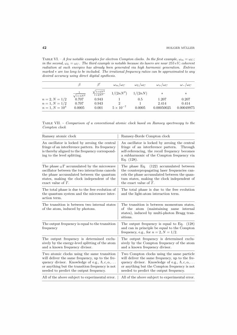
42 HOLGER MULLER
Table VI. – A few notable examples for electron Compton clocks. In the first example, ωm = ωC ;in the second, ωL = ωC . The third example is notable because its lasers are near 255 eV; coherentradiation at such energies has already been generated via high harmonic generation. Entriesmarked ∗ are too long to be included. The irrational frequency ratios can be approximated to anydesired accuracy using direct digital synthesis.
β β′ ωm/ωC ωL/ωC ω+/ωC ω−/ωC
1√1+4N2
√1+4N2
1+2N2 1/(2nN2) 1/(2nN) ∗ ∗n = 2, N = 1/2 0.707 0.943 1 0.5 1.207 0.207n = 1, N = 1/2 0.707 0.943 2 1 2.414 0.414n = 1, N = 103 0.0005 0.001 5× 10⁻⁷ 0.0005 0.00050025 0.00049975
Table VII. – Comparison of a conventional atomic clock based on Ramsey spectrocopy to theCompton clock
Ramsey atomic clock Ramsey-Borde Compton clock
An oscillator is locked by zeroing the centralfringe of an interference pattern. Its frequencyis thereby aligned to the frequency correspond-ing to the level splitting.
An oscillator is locked by zeroing the centralfringe of an interference pattern. Throughself-referencing, the recoil frequency becomesa subharmonic of the Compton frequency viaEq. (128).
The phase ωT accumulated by the microwaveoscillator between the two interactions cancelsthe phase accumulated between the quantumstates, making the clock independent of theexact value of T .
The phase Eq. (122) accumulated betweenthe counterpropagating laser frequencies can-cels the phase accumulated between the quan-tum states, making the clock independent ofthe exact value of T .
The total phase is due to the free evolution ofthe quantum system and the microwave inter-action term.
The total phase is due to the free evolutionand the light-atom interaction term.
The transition is between two internal statesof the atom, induced by photons.
The transition is between momentum states,of the atom (maintaining same internalstates), induced by multi-photon Bragg tran-sitions.
The output frequency is equal to the transitionfrequency
The output frequency is equal to Eq. (128)and can in principle be equal to the Comptonfrequency, e.g., for n = 2, N = 1/2.
The output frequency is determined exclu-sively by the energy-level splitting of the atomand a known frequency divisor.
The output frequency is determined exclu-sively by the Compton frequency of the atomand a known frequency divisor.
Two atomic clocks using the same transitionwill deliver the same frequency, up to the fre-quency divisor. Knowledge of e.g., ~, c, α, . . .or anything but the transition frequency is notneeded to predict the output frequency.
Two Compton clocks using the same particlewill deliver the same frequency, up to the fre-quency divisor. Knowledge of e.g., ~, c, α, . . .or anything but the Compton frequency is notneeded to predict the output frequency.
All of the above subject to experimental error. All of the above subject to experimental error.
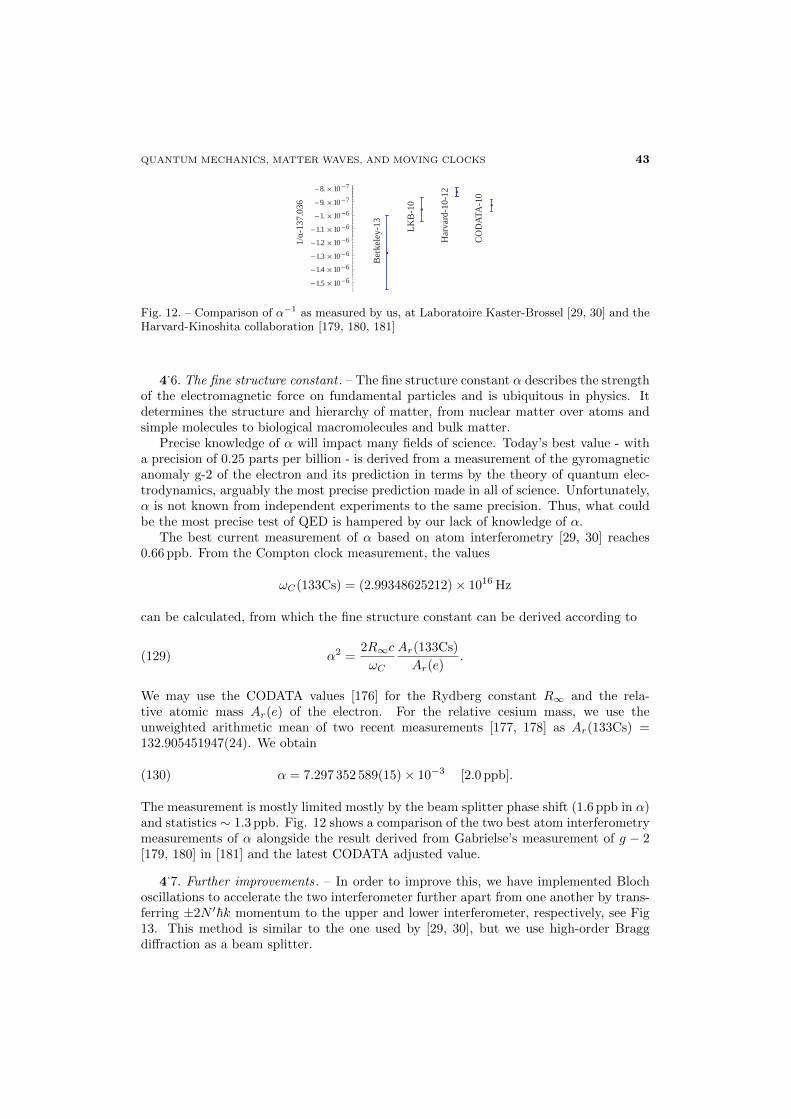
QUANTUM MECHANICS, MATTER WAVES, AND MOVING CLOCKS 43
78. 10 7
-12 0
1.1 10 61. 10 69. 10 7
ey-1
3
LKB
-10
Har
vard
-10-
CO
DAT
A-1
0
-137
.036
1.4 10 61.3 10 61.2 10 6
Ber
kele H C1/
1.5 10 6
Fig. 12. – Comparison of α−1 as measured by us, at Laboratoire Kaster-Brossel [29, 30] and theHarvard-Kinoshita collaboration [179, 180, 181]
4.6. The fine structure constant . – The fine structure constant α describes the strength
of the electromagnetic force on fundamental particles and is ubiquitous in physics. Itdetermines the structure and hierarchy of matter, from nuclear matter over atoms andsimple molecules to biological macromolecules and bulk matter.
Precise knowledge of α will impact many fields of science. Today’s best value - witha precision of 0.25 parts per billion - is derived from a measurement of the gyromagneticanomaly g-2 of the electron and its prediction in terms by the theory of quantum elec-trodynamics, arguably the most precise prediction made in all of science. Unfortunately,α is not known from independent experiments to the same precision. Thus, what couldbe the most precise test of QED is hampered by our lack of knowledge of α.
The best current measurement of α based on atom interferometry [29, 30] reaches0.66 ppb. From the Compton clock measurement, the values
ωC(133Cs) = (2.99348625212)× 1016 Hz
can be calculated, from which the fine structure constant can be derived according to
(129) α2 =2R∞cωC
Ar(133Cs)
Ar(e).
We may use the CODATA values [176] for the Rydberg constant R∞ and the rela-tive atomic mass Ar(e) of the electron. For the relative cesium mass, we use theunweighted arithmetic mean of two recent measurements [177, 178] as Ar(133Cs) =132.905451947(24). We obtain
(130) α = 7.297 352 589(15)× 10−3 [2.0 ppb].
The measurement is mostly limited mostly by the beam splitter phase shift (1.6 ppb in α)and statistics ∼ 1.3 ppb. Fig. 12 shows a comparison of the two best atom interferometrymeasurements of α alongside the result derived from Gabrielse’s measurement of g − 2[179, 180] in [181] and the latest CODATA adjusted value.
4.7. Further improvements. – In order to improve this, we have implemented Bloch
oscillations to accelerate the two interferometer further apart from one another by trans-ferring ±2N ′~k momentum to the upper and lower interferometer, respectively, see Fig13. This method is similar to the one used by [29, 30], but we use high-order Braggdiffraction as a beam splitter.
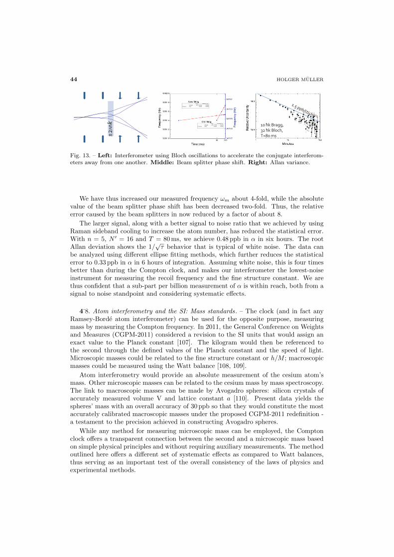
44 HOLGER MULLER
±2Nħk
10 ħk Bragg, 32 ħk Bloch, T=80 ms
Fig. 13. – Left: Interferometer using Bloch oscillations to accelerate the conjugate interferom-eters away from one another. Middle: Beam splitter phase shift. Right: Allan variance.
We have thus increased our measured frequency ωm about 4-fold, while the absolutevalue of the beam splitter phase shift has been decreased two-fold. Thus, the relativeerror caused by the beam splitters in now reduced by a factor of about 8.
The larger signal, along with a better signal to noise ratio that we achieved by usingRaman sideband cooling to increase the atom number, has reduced the statistical error.With n = 5, N ′ = 16 and T = 80 ms, we achieve 0.48 ppb in α in six hours. The rootAllan deviation shows the 1/
√τ behavior that is typical of white noise. The data can
be analyzed using different ellipse fitting methods, which further reduces the statisticalerror to 0.33 ppb in α in 6 hours of integration. Assuming white noise, this is four timesbetter than during the Compton clock, and makes our interferometer the lowest-noiseinstrument for measuring the recoil frequency and the fine structure constant. We arethus confident that a sub-part per billion measurement of α is within reach, both from asignal to noise standpoint and considering systematic effects.
4.8. Atom interferometry and the SI: Mass standards. – The clock (and in fact any
Ramsey-Borde atom interferometer) can be used for the opposite purpose, measuringmass by measuring the Compton frequency. In 2011, the General Conference on Weightsand Measures (CGPM-2011) considered a revision to the SI units that would assign anexact value to the Planck constant [107]. The kilogram would then be referenced tothe second through the defined values of the Planck constant and the speed of light.Microscopic masses could be related to the fine structure constant or h/M ; macroscopicmasses could be measured using the Watt balance [108, 109].
Atom interferometry would provide an absolute measurement of the cesium atom’smass. Other microscopic masses can be related to the cesium mass by mass spectroscopy.The link to macroscopic masses can be made by Avogadro spheres: silicon crystals ofaccurately measured volume V and lattice constant a [110]. Present data yields thespheres’ mass with an overall accuracy of 30 ppb so that they would constitute the mostaccurately calibrated macroscopic masses under the proposed CGPM-2011 redefinition -a testament to the precision achieved in constructing Avogadro spheres.
While any method for measuring microscopic mass can be employed, the Comptonclock offers a transparent connection between the second and a microscopic mass basedon simple physical principles and without requiring auxiliary measurements. The methodoutlined here offers a different set of systematic effects as compared to Watt balances,thus serving as an important test of the overall consistency of the laws of physics andexperimental methods.
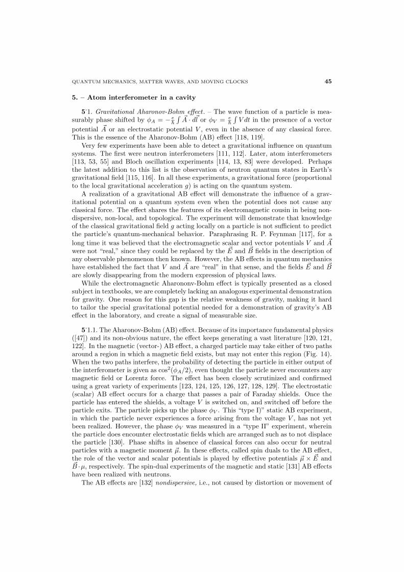
QUANTUM MECHANICS, MATTER WAVES, AND MOVING CLOCKS 45
5. – Atom interferometer in a cavity
5.1. Gravitational Aharonov-Bohm effect . – The wave function of a particle is mea-
surably phase shifted by φA = − e~∫~A · d~l or φV = e
~∫V dt in the presence of a vector
potential ~A or an electrostatic potential V , even in the absence of any classical force.This is the essence of the Aharonov-Bohm (AB) effect [118, 119].
Very few experiments have been able to detect a gravitational influence on quantumsystems. The first were neutron interferometers [111, 112]. Later, atom interferometers[113, 53, 55] and Bloch oscillation experiments [114, 13, 83] were developed. Perhapsthe latest addition to this list is the observation of neutron quantum states in Earth’sgravitational field [115, 116]. In all these experiments, a gravitational force (proportionalto the local gravitational acceleration g) is acting on the quantum system.
A realization of a gravitational AB effect will demonstrate the influence of a grav-itational potential on a quantum system even when the potential does not cause anyclassical force. The effect shares the features of its electromagnetic cousin in being non-dispersive, non-local, and topological. The experiment will demonstrate that knowledgeof the classical gravitational field g acting locally on a particle is not sufficient to predictthe particle’s quantum-mechanical behavior. Paraphrasing R. P. Feynman [117], for a
long time it was believed that the electromagnetic scalar and vector potentials V and ~Awere not “real,” since they could be replaced by the ~E and ~B fields in the description ofany observable phenomenon then known. However, the AB effects in quantum mechanicshave established the fact that V and ~A are “real” in that sense, and the fields ~E and ~Bare slowly disappearing from the modern expression of physical laws.
While the electromagnetic Aharononv-Bohm effect is typically presented as a closedsubject in textbooks, we are completely lacking an analogous experimental demonstrationfor gravity. One reason for this gap is the relative weakness of gravity, making it hardto tailor the special gravitational potential needed for a demonstration of gravity’s ABeffect in the laboratory, and create a signal of measurable size.
5.1.1. The Aharonov-Bohm (AB) effect. Because of its importance fundamental physics
([47]) and its non-obvious nature, the effect keeps generating a vast literature [120, 121,122]. In the magnetic (vector-) AB effect, a charged particle may take either of two pathsaround a region in which a magnetic field exists, but may not enter this region (Fig. 14).When the two paths interfere, the probability of detecting the particle in either output ofthe interferometer is given as cos2(φA/2), even thought the particle never encounters anymagnetic field or Lorentz force. The effect has been closely scrutinized and confirmedusing a great variety of experiments [123, 124, 125, 126, 127, 128, 129]. The electrostatic(scalar) AB effect occurs for a charge that passes a pair of Faraday shields. Once theparticle has entered the shields, a voltage V is switched on, and switched off before theparticle exits. The particle picks up the phase φV . This “type I)” static AB experiment,in which the particle never experiences a force arising from the voltage V , has not yetbeen realized. However, the phase φV was measured in a “type II” experiment, whereinthe particle does encounter electrostatic fields which are arranged such as to not displacethe particle [130]. Phase shifts in absence of classical forces can also occur for neutralparticles with a magnetic moment ~µ. In these effects, called spin duals to the AB effect,the role of the vector and scalar potentials is played by effective potentials ~µ × ~E and~B ·µ, respectively. The spin-dual experiments of the magnetic and static [131] AB effectshave been realized with neutrons.
The AB effects are [132] nondispersive, i.e., not caused by distortion or movement of
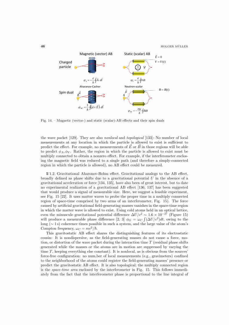
46 HOLGER MULLER
Magnetic (vector) AB Static (scalar) AB
ldAeA
V
VdteV
e
ldEAC1
Spin dual
BdtNS
)(0
tVVE
Aharanov-Casher Neutron-scalar
Charged particle VVVVVVVe
n
)(tBB
n
Fig. 14. – Magnetic (vector-) and static (scalar)-AB effects and their spin duals
the wave packet [129]. They are also nonlocal and topological [133]: No number of localmeasurements at any location in which the particle is allowed to exist is sufficient topredict the effect. For example, no measurements of ~E or ~B in those regions will be ableto predict φA, φV . Rather, the region in which the particle is allowed to exist must bemultiply connected to obtain a nonzero effect. For example, if the interferometer enclos-ing the magnetic field was reduced to a single path (and therefore a simply-connectedregion in which the particle is allowed), no AB effect could be measured.
5.1.2. Gravitational Aharonov-Bohm effect. Gravitational analogs to the AB effect,
broadly defined as phase shifts due to a gravitational potential U in the absence of agravitational acceleration or force [134, 135], have also been of great interest, but to dateno experimental realization of a gravitational AB effect [136, 137] has been suggestedthat would produce a signal of measurable size. Here, we suggest a feasible experiment,see Fig. 15 [22]. It uses matter waves to probe the proper time in a multiply connectedregion of space-time comprised by two arms of an interferometer, Fig. 15). The forcecaused by artificial gravitational field-generating masses vanishes in the space-time regionin which the matter wave is allowed to exist. Using cold atoms held in an optical lattice,even the minuscule gravitational potential difference ∆U/c2 ∼ 1.6 × 10⁻²⁷ (Figure 15)will produce a measurable phase difference [2, 3] φG = ωC
∫(∆U/c2)dt, owing to the
long (∼ 1 s) coherence times possible in such a system, and the large value of the atom’sCompton frequency, ωC = mc2/~.
This gravitostatic AB effect shares the distinguishing features of its electrostaticcousin: It is nondispersive, as the field-generating masses do not cause a force, mo-tion, or distortion of the wave packet during the interaction time T (residual phase shiftsgenerated while the masses or the atoms are in motion are suppressed by varying thetime T , keeping everything else constant). It is nonlocal, as is obvious from the sources’force-free configuration: no num,ber of local measurements (e.g., gravimeters) confinedto the neighborhood of the atoms could register the field-generating masses’ presence orpredict the gravitostatic AB effect. It is also topological; the multiply connected regionis the space-time area enclosed by the interferometer in Fig. 15. This follows immedi-ately from the fact that the interferometer phase is proportional to the line integral of
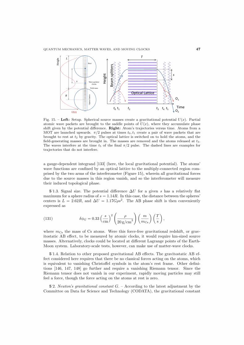
QUANTUM MECHANICS, MATTER WAVES, AND MOVING CLOCKS 47
Opt
ical
latti
ce
Field mass
Wave packets/ clocks
Bore
s
L
R
U(x)
Hei
ght
Optical Lattice
Beam
spl
itter
s Time
Hei
ght
t0 t1 t2 t3 t4 t5
T
s
O1
O2
Fig. 15. – Left: Setup. Spherical source masses create a gravitational potential U(x). Partialatomic wave packets are brought to the saddle points of U(x), where they accumulate phaseshift given by the potential difference. Right: Atom’s trajectories versus time. Atoms from aMOT are launched upwards. π/2 pulses at times t0, t1 create a pair of wave packets that arebrought to rest at t2 by gravity. The optical lattice is switched on to hold the atoms, and thefield-generating masses are brought in. The masses are removed and the atoms released at t3.The waves interfere at the time t5 of the final π/2 pulse. The dashed lines are examples fortrajectories that do not interfere.
a gauge-dependent integrand [133] (here, the local gravitational potential). The atoms’wave functions are confined by an optical lattice to the multiply-connected region com-prised by the two arms of the interferometer (Figure 15), wherein all gravitational forcesdue to the source masses in this region vanish, and so the interferometer will measuretheir induced topological phase.
5.1.3. Signal size. The potential difference ∆U for a given s has a relatively flat
maximum for a sphere radius of s = 1.14R. In this case, the distance between the spheres’centers is L = 2.62R, and ∆U = 1.17Gρs2. The AB phase shift is then convenientlyexpressed as
(131) δφG = 0.33( s
cm
)2(
ρ
20 g/cm3
)(m
mCs
)(T
s
),
where mCs the mass of Cs atoms. Were this force-free gravitational redshift, or grav-itostatic AB effect, to be measured by atomic clocks, it would require km-sized sourcemasses. Alternatively, clocks could be located at different Lagrange points of the Earth-Moon system. Laboratory-scale tests, however, can make use of matter-wave clocks.
5.1.4. Relation to other proposed gravitational AB effects. The gravitostatic AB ef-
fect considered here requires that there be no classical forces acting on the atoms, whichis equivalent to vanishing Christoffel symbols in the atom’s rest frame. Other defini-tions [146, 147, 148] go further and require a vanishing Riemann tensor. Since theRiemann tensor does not vanish in our experiment, rapidly moving particles may stillfeel a force, though the force acting on the atoms at rest is zero.
5.2. Newton’s gravitational constant G. – According to the latest adjustment by the
Committee on Data for Science and Technology (CODATA), the gravitational constant
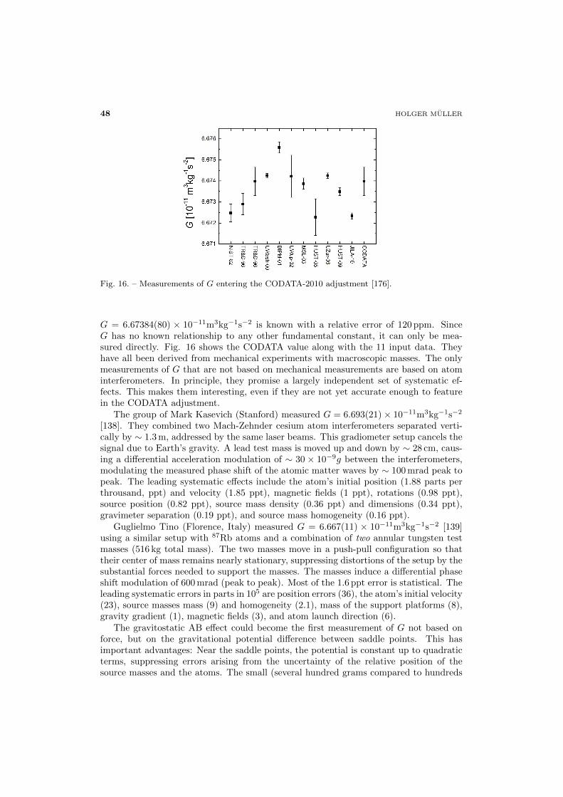
48 HOLGER MULLER
Fig. 16. – Measurements of G entering the CODATA-2010 adjustment [176].
G = 6.67384(80) × 10−11m3kg−1s−2 is known with a relative error of 120 ppm. SinceG has no known relationship to any other fundamental constant, it can only be mea-sured directly. Fig. 16 shows the CODATA value along with the 11 input data. Theyhave all been derived from mechanical experiments with macroscopic masses. The onlymeasurements of G that are not based on mechanical measurements are based on atominterferometers. In principle, they promise a largely independent set of systematic ef-fects. This makes them interesting, even if they are not yet accurate enough to featurein the CODATA adjustment.
The group of Mark Kasevich (Stanford) measured G = 6.693(21)× 10−11m3kg−1s−2
[138]. They combined two Mach-Zehnder cesium atom interferometers separated verti-cally by ∼ 1.3 m, addressed by the same laser beams. This gradiometer setup cancels thesignal due to Earth’s gravity. A lead test mass is moved up and down by ∼ 28 cm, caus-ing a differential acceleration modulation of ∼ 30 × 10−9g between the interferometers,modulating the measured phase shift of the atomic matter waves by ∼ 100 mrad peak topeak. The leading systematic effects include the atom’s initial position (1.88 parts perthrousand, ppt) and velocity (1.85 ppt), magnetic fields (1 ppt), rotations (0.98 ppt),source position (0.82 ppt), source mass density (0.36 ppt) and dimensions (0.34 ppt),gravimeter separation (0.19 ppt), and source mass homogeneity (0.16 ppt).
Guglielmo Tino (Florence, Italy) measured G = 6.667(11) × 10−11m3kg−1s−2 [139]using a similar setup with 87Rb atoms and a combination of two annular tungsten testmasses (516 kg total mass). The two masses move in a push-pull configuration so thattheir center of mass remains nearly stationary, suppressing distortions of the setup by thesubstantial forces needed to support the masses. The masses induce a differential phaseshift modulation of 600 mrad (peak to peak). Most of the 1.6 ppt error is statistical. Theleading systematic errors in parts in 105 are position errors (36), the atom’s initial velocity(23), source masses mass (9) and homogeneity (2.1), mass of the support platforms (8),gravity gradient (1), magnetic fields (3), and atom launch direction (6).
The gravitostatic AB effect could become the first measurement of G not based onforce, but on the gravitational potential difference between saddle points. This hasimportant advantages: Near the saddle points, the potential is constant up to quadraticterms, suppressing errors arising from the uncertainty of the relative position of thesource masses and the atoms. The small (several hundred grams compared to hundreds
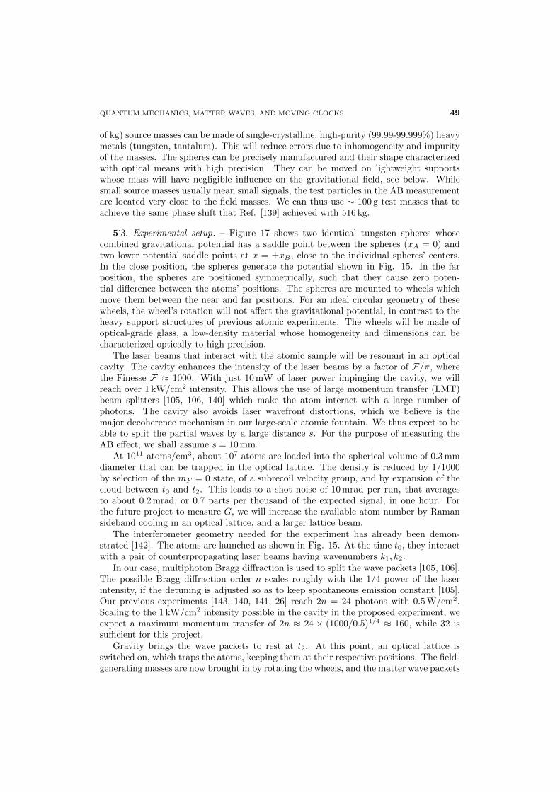
QUANTUM MECHANICS, MATTER WAVES, AND MOVING CLOCKS 49
of kg) source masses can be made of single-crystalline, high-purity (99.99-99.999%) heavymetals (tungsten, tantalum). This will reduce errors due to inhomogeneity and impurityof the masses. The spheres can be precisely manufactured and their shape characterizedwith optical means with high precision. They can be moved on lightweight supportswhose mass will have negligible influence on the gravitational field, see below. Whilesmall source masses usually mean small signals, the test particles in the AB measurementare located very close to the field masses. We can thus use ∼ 100 g test masses that toachieve the same phase shift that Ref. [139] achieved with 516 kg.
5.3. Experimental setup. – Figure 17 shows two identical tungsten spheres whose
combined gravitational potential has a saddle point between the spheres (xA = 0) andtwo lower potential saddle points at x = ±xB , close to the individual spheres’ centers.In the close position, the spheres generate the potential shown in Fig. 15. In the farposition, the spheres are positioned symmetrically, such that they cause zero poten-tial difference between the atoms’ positions. The spheres are mounted to wheels whichmove them between the near and far positions. For an ideal circular geometry of thesewheels, the wheel’s rotation will not affect the gravitational potential, in contrast to theheavy support structures of previous atomic experiments. The wheels will be made ofoptical-grade glass, a low-density material whose homogeneity and dimensions can becharacterized optically to high precision.
The laser beams that interact with the atomic sample will be resonant in an opticalcavity. The cavity enhances the intensity of the laser beams by a factor of F/π, wherethe Finesse F ≈ 1000. With just 10 mW of laser power impinging the cavity, we willreach over 1 kW/cm2 intensity. This allows the use of large momentum transfer (LMT)beam splitters [105, 106, 140] which make the atom interact with a large number ofphotons. The cavity also avoids laser wavefront distortions, which we believe is themajor decoherence mechanism in our large-scale atomic fountain. We thus expect to beable to split the partial waves by a large distance s. For the purpose of measuring theAB effect, we shall assume s = 10 mm.
At 1011 atoms/cm3, about 107 atoms are loaded into the spherical volume of 0.3 mmdiameter that can be trapped in the optical lattice. The density is reduced by 1/1000by selection of the mF = 0 state, of a subrecoil velocity group, and by expansion of thecloud between t0 and t2. This leads to a shot noise of 10 mrad per run, that averagesto about 0.2 mrad, or 0.7 parts per thousand of the expected signal, in one hour. Forthe future project to measure G, we will increase the available atom number by Ramansideband cooling in an optical lattice, and a larger lattice beam.
The interferometer geometry needed for the experiment has already been demon-strated [142]. The atoms are launched as shown in Fig. 15. At the time t0, they interactwith a pair of counterpropagating laser beams having wavenumbers k1, k2.
In our case, multiphoton Bragg diffraction is used to split the wave packets [105, 106].The possible Bragg diffraction order n scales roughly with the 1/4 power of the laserintensity, if the detuning is adjusted so as to keep spontaneous emission constant [105].Our previous experiments [143, 140, 141, 26] reach 2n = 24 photons with 0.5 W/cm2.Scaling to the 1 kW/cm2 intensity possible in the cavity in the proposed experiment, weexpect a maximum momentum transfer of 2n ≈ 24 × (1000/0.5)1/4 ≈ 160, while 32 issufficient for this project.
Gravity brings the wave packets to rest at t2. At this point, an optical lattice isswitched on, which traps the atoms, keeping them at their respective positions. The field-generating masses are now brought in by rotating the wheels, and the matter wave packets
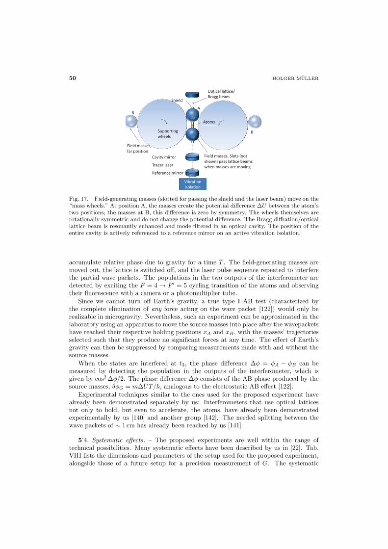
50 HOLGER MULLER
A
B
B
Optical lattice/ Bragg beam
Supporting wheels
Field masses. Slots (not shown) pass lattice beams when masses are moving
Atoms
Cavity mirror
Field masses, far position
Shield
Vibration isolation
Reference mirror
Tracer laser
Fig. 17. – Field-generating masses (slotted for passing the shield and the laser beam) move on the“mass wheels.” At position A, the masses create the potential difference ∆U between the atom’stwo positions; the masses at B, this difference is zero by symmetry. The wheels themselves arerotationally symmetric and do not change the potential difference. The Bragg diffration/opticallattice beam is resonantly enhanced and mode filtered in an optical cavity. The position of theentire cavity is actively referenced to a reference mirror on an active vibration isolation.
accumulate relative phase due to gravity for a time T . The field-generating masses aremoved out, the lattice is switched off, and the laser pulse sequence repeated to interferethe partial wave packets. The populations in the two outputs of the interferometer aredetected by exciting the F = 4 → F ′ = 5 cycling transition of the atoms and observingtheir fluorescence with a camera or a photomultiplier tube.
Since we cannot turn off Earth’s gravity, a true type I AB test (characterized bythe complete elimination of any force acting on the wave packet [122]) would only berealizable in microgravity. Nevertheless, such an experiment can be approximated in thelaboratory using an apparatus to move the source masses into place after the wavepacketshave reached their respective holding positions xA and xB , with the masses’ trajectoriesselected such that they produce no significant forces at any time. The effect of Earth’sgravity can then be suppressed by comparing measurements made with and without thesource masses.
When the states are interfered at t3, the phase difference ∆φ = φA − φB can bemeasured by detecting the population in the outputs of the interferometer, which isgiven by cos2 ∆φ/2. The phase difference ∆φ consists of the AB phase produced by thesource masses, δφG = m∆UT/~, analogous to the electrostatic AB effect [122].
Experimental techniques similar to the ones used for the proposed experiment havealready been demonstrated separately by us: Interferometers that use optical latticesnot only to hold, but even to accelerate, the atoms, have already been demonstratedexperimentally by us [140] and another group [142]. The needed splitting between thewave packets of ∼ 1 cm has already been reached by us [141].
5.4. Systematic effects. – The proposed experiments are well within the range of
technical possibilities. Many systematic effects have been described by us in [22]. Tab.VIII lists the dimensions and parameters of the setup used for the proposed experiment,alongside those of a future setup for a precision measurement of G. The systematic
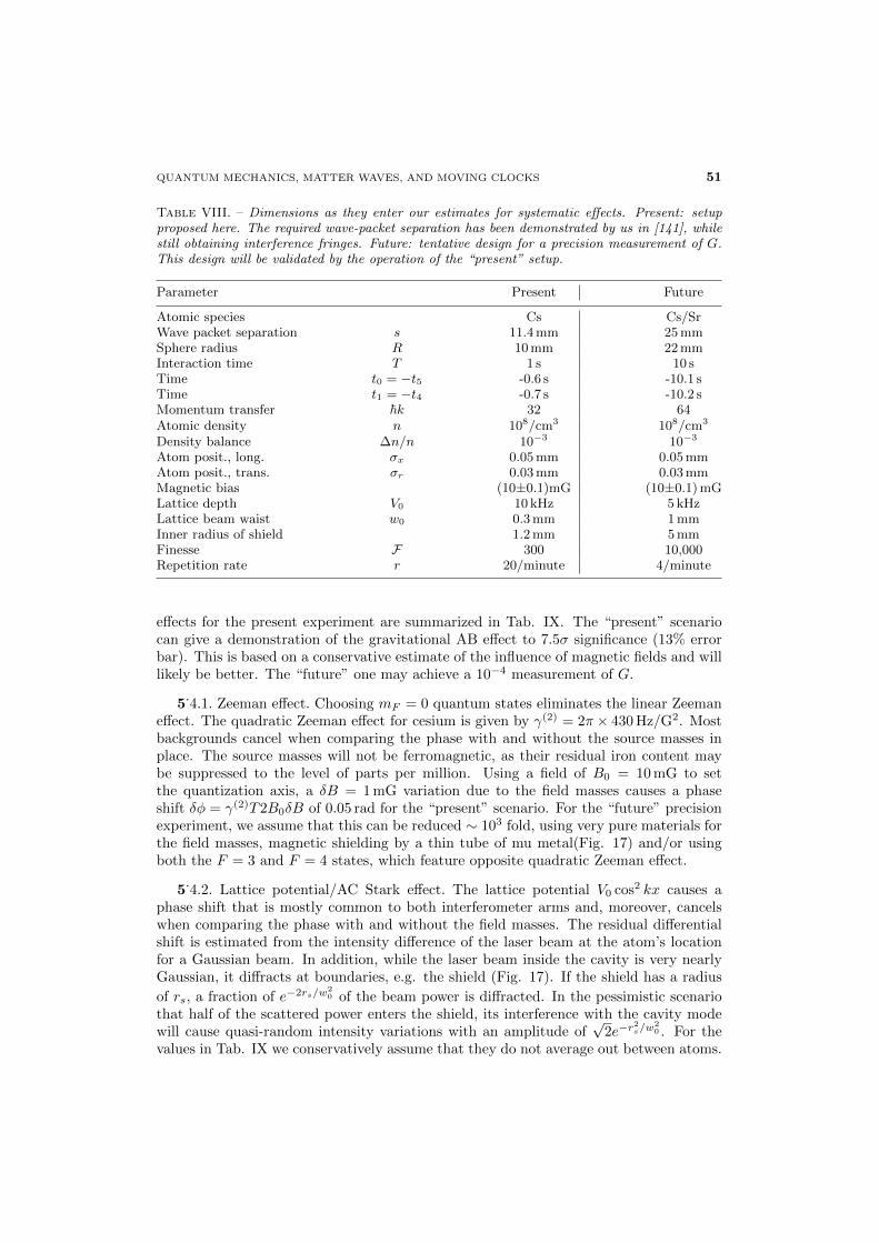
QUANTUM MECHANICS, MATTER WAVES, AND MOVING CLOCKS 51
Table VIII. – Dimensions as they enter our estimates for systematic effects. Present: setupproposed here. The required wave-packet separation has been demonstrated by us in [141], whilestill obtaining interference fringes. Future: tentative design for a precision measurement of G.This design will be validated by the operation of the “present” setup.
Parameter Present Future
Atomic species Cs Cs/SrWave packet separation s 11.4 mm 25 mmSphere radius R 10 mm 22 mmInteraction time T 1 s 10 sTime t0 = −t5 -0.6 s -10.1 sTime t1 = −t4 -0.7 s -10.2 sMomentum transfer ~k 32 64Atomic density n 108/cm3 108/cm3
Density balance ∆n/n 10−3 10−3
Atom posit., long. σx 0.05 mm 0.05 mmAtom posit., trans. σr 0.03 mm 0.03 mmMagnetic bias (10±0.1)mG (10±0.1) mGLattice depth V0 10 kHz 5 kHzLattice beam waist w0 0.3 mm 1 mmInner radius of shield 1.2 mm 5 mmFinesse F 300 10,000Repetition rate r 20/minute 4/minute
effects for the present experiment are summarized in Tab. IX. The “present” scenariocan give a demonstration of the gravitational AB effect to 7.5σ significance (13% errorbar). This is based on a conservative estimate of the influence of magnetic fields and willlikely be better. The “future” one may achieve a 10−4 measurement of G.
5.4.1. Zeeman effect. Choosing mF = 0 quantum states eliminates the linear Zeeman
effect. The quadratic Zeeman effect for cesium is given by γ(2) = 2π × 430 Hz/G2. Mostbackgrounds cancel when comparing the phase with and without the source masses inplace. The source masses will not be ferromagnetic, as their residual iron content maybe suppressed to the level of parts per million. Using a field of B0 = 10 mG to setthe quantization axis, a δB = 1 mG variation due to the field masses causes a phaseshift δφ = γ(2)T2B0δB of 0.05 rad for the “present” scenario. For the “future” precisionexperiment, we assume that this can be reduced ∼ 103 fold, using very pure materials forthe field masses, magnetic shielding by a thin tube of mu metal(Fig. 17) and/or usingboth the F = 3 and F = 4 states, which feature opposite quadratic Zeeman effect.
5.4.2. Lattice potential/AC Stark effect. The lattice potential V0 cos2 kx causes a
phase shift that is mostly common to both interferometer arms and, moreover, cancelswhen comparing the phase with and without the field masses. The residual differentialshift is estimated from the intensity difference of the laser beam at the atom’s locationfor a Gaussian beam. In addition, while the laser beam inside the cavity is very nearlyGaussian, it diffracts at boundaries, e.g. the shield (Fig. 17). If the shield has a radius
of rs, a fraction of e−2rs/w20 of the beam power is diffracted. In the pessimistic scenario
that half of the scattered power enters the shield, its interference with the cavity modewill cause quasi-random intensity variations with an amplitude of
√2e−r
2s/w
20 . For the
values in Tab. IX we conservatively assume that they do not average out between atoms.
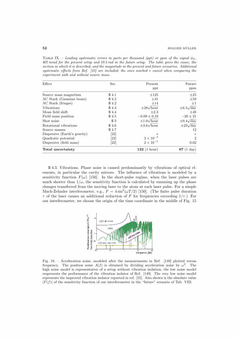
52 HOLGER MULLER
Table IX. – Leading systematic errors in parts per thousand (ppt) or ppm of the signal φG,407 mrad for the present setup and 19.5 rad in the future setup. The table gives the cause, thesection in which it is described, and the magnitude in the present and future scenarios. Additionalsystematic effects from Ref. [22] are included; the ones marked ∗ cancel when comparing theexperiment with and without source mass.
Effect Sec. Present Futureppt ppm
Source mass magnetism 5.4.1 ±125 ±25
AC Stark (Gaussian beam) 5.4.2 ±31 ±59
AC Stark (fringes) 5.4.2 ±14 ±1
Vibrations 5.4.3 ±28
√hour ±6.5
√day
Mean field shift 5.4.4 ±2.3 ±48
Field mass position 5.4.5 −0.09± 0.10 −20± 21
Shot noise 5.3 ±1.0
√hour ±0.4
√day
Rotational vibrations 5.4.6 ±3.6
√hour ±23
√day
Source masses 5.4.7 12
Dispersive (Earth’s gravity) [22] ∗ ∗Quadratic potential [22] 2× 10⁻³ 2Dispersive (field mass) [22] 2× 10⁻⁵ 0.02
Total uncertainty 132 (1 hour) 87 (1 day)
5.4.3. Vibrations. Phase noise is caused predominantly by vibrations of optical el-
ements, in particular the cavity mirrors. The influence of vibrations is modeled by asensitivity function F (ω) [150]. In the short-pulse regime, when the laser pulses aremuch shorter than 1/ω, the sensitivity function is calculated by summing up the phasechanges transferred from the moving laser to the atom at each laser pulse. For a simpleMach-Zehnder interferometer, e.g., F = 4 sin2(ωT/2) [150]. (The finite pulse durationτ of the laser causes an additional reduction of F for frequencies exceeding 1/τ .) Forour interferometer, we choose the origin of the time coordinate in the middle of Fig. 15
Fig. 18. – Acceleration noise, modeled after the measurements in Ref. [149] plotted versusfrequency. The position noise A(f) is obtained by dividing acceleration noise by ω2. Thehigh noise model is representative of a setup without vibration isolation, the low noise modelrespresents the performance of the vibration isolator of Ref. [149]. The very low noise modelrepresents the improved vibration isolator reported in ref. [55]. Also shown is the absolute value|F (f)| of the sensitivity function of our interferometer in the “future” scenario of Tab. VIII.
QUANTUM MECHANICS, MATTER WAVES, AND MOVING CLOCKS 53
(right), such that t0 = −t5, t1 = −t4, t2 = −t3. The optical lattice section does not,to leading order, transfer phase noise to the atomic wave function because any actionof the lattice is common-mode to both interferometer arms. (Vibrations much strongerthan those relevant here would drive transitions to higher lattice bands, causing loss ofcontrast.) We find F (ω) = −[x(t0) + x(t1) + x(t4)− x(t5)] or
(132) F (ω) = 4 sin
(ωt0 + t1
2
)sin
(ωt0 − t1
2
).
The second sine function means that frequencies below 1/|t0 − t1| are suppressed, whichsimplifies the vibration isolation considerably.
The “high noise” and “low noise” graphs in Fig. 18 show an analytic representationof acceleration noise a(ω) measured on a typical optical table (next to an operatingair conditioning unit) with and without active vibration isolation [149], alongside thesensitivity function F . We obtain the total noise affecting the experiment by noting thatthe position noise A(ω) = a(ω)/ω2 and integrating keff [
∫∞0
(a(ω)F (ω)/ω2)2dω]1/2.In the present scenario, the high-noise model predicts an effective rms phase noise
of 105 rad, making it impossible to see interference. Vibration isolation can reduce thisnoise: The low noise model (Fig. 18) predicts an effective rms phase noise of 0.39 radso that fringes can be observed. The experiment can be repeated 1200 times per hour,allowing to average the vibration-induced noise down to 28 parts per thousand of theexpected signal. For the future scenario we expect to be able to reduce the noise to thelevel of Ref. [55], as represented by the “very low noise model.” The predicted effectivephase noise is then 0.1 rad.
5.4.4. Mean field shift. Atom-atom interactions produce a phase shift 4π~anT/m,
where a ∼ 3000a0 is the scattering length of Cs atoms (a0 is the Bohr radius) and n isthe atomic density. Systematic effects are caused by a difference in atomic densities ∆ncorrelated with the position of the field-generating masses. We know of no mechanismthat would cause such correlations and thus assume they are 0.1% or less, obtaining theestimate given in Tab IX.
5.4.5. Test masses and atom positions. We consider the gravitational potential due
to test masses in the geometry of Fig. 15, i.e, L = 2.62R. We assume that deviationsof the atom positions from the maximum and minimum saddle points (δx)max, (δx)min
longitudinally and (δr)max, (δr)min transversally are taken from Gaussian distributionscentered at zero with variances σz, σr, respectively. Second-order expansion of the po-tential leads to an expectation value 〈δφ〉 of the phase shift of (0.04σ2
r − 3.89σ2x)/R2 and
a variance of√
5.76σ4r + 16.11σ4
x/R2 and leads to the estimates in Tab. IX.
5.4.6. Rotations. The one-dimensional vibration-isolation system cannot eliminate
rotational vibrations. Ideally, the planned interferometer does not enclose a spatial area(rather than a space-time area), as there is no horizontal velocity component of the
atoms. The interferometer is thus insensitive to rotations ~Ω to leading order. Theresidual influence scales with the induced displacement ~δr of the optical lattices relativeto the (inertial) matter wave packets, which causes a phase shift ~keff · ~δr. During theoptical lattice holding time T , the atoms do not move relative to the lattice, so therelevant time scale is given by t1 − t0. We thus arrive at an order-of-magnitude phaseshift of (~keff × ~v0) · Ω(t1 − t0). For an estimate of v0, the velocity v0 must be less thanw0/T if the atoms are to be held in the lattice of waist w0. Rotational noise is typically
54 HOLGER MULLER
much lower than Earth’s rotation rate Ω⊕ [141]. Assuming vibrational noise amounts toless than Ω⊕/10 rms, we obtain the estimates in Tab. IX.
The constant rotation rate of the Earth is irrelevant, as it is suppressed when takingthe difference between experiments with the source masses and without.
5.4.7. Source masses. In [139], the most precise measurement of G with atom interfer-
ometry to date, source masses consisted of 24 tungsten cylinders and contributed an errorof 90 ppm through their mass and 21 ppm through their homogeneity. Additional errors(80 ppm) were due to the mass of the support platforms. The small (hundreds of gramsversus hundreds of kg), spherical source masses can be made out of high-purity, crys-talline material and thus extremely homogenous and their shape well controlled. Whilethe measurement of G will not be performed as part of the propsed work, we expect thatthese errors can be improved tenfold.
5.5. Matter waves and the measurement of proper time. – The experiment will unam-
biguously demonstrate that matter-waves are not merely classical point masses that pro-vide quantum measurements of the gravitational acceleration: a matter-wave is subjectto the same gravitational redshift and time-dilation effects that apply to a conventionalclock, even if it is constrained to a space time region of vanishing gravitational force. Theproposed experiment will be the first demonstration of a force-free gravitational redshift,and the first experimental demonstration of a gravitostatic AB effect. The effect is non-dispersive and topological, and thus impossible to ascribe to any local influences on thewave packet. This rules out interpretations that ascribe the phase entirely to the phaseof the diffraction gratings at the positions of the wave packets [39, 40, 41].
6. – Antimatter interferometry
The Antihydrogen Laser Physics Apparatus (ALPHA) has reported groundbreakingresults in antihydrogen physics over the past few years: the world’s first trapped antihy-drogen [151], confinement of antihydrogen for 1,000 seconds or more [152], and hyperfinespectroscopy of antihydrogen [153]. It has already conducted a pioneering measure-ment which constrained the gravitational acceleration of antihydrogen to a range of−0.7 . . . + 1.1 km/s2 [154]. The methods used, however, are not suitable for precisionmeasurements; at best, they may tell us whether antihydrogen will rise or fall in Earth’sgravitational field. The apparatus described here [155] should be capable of precision atinitially the 1% level of precision and, with upgrades, the 10−6 level. We assume thatanti-atoms will be laser-cooled to a temperature of 20 mK [156] and that a new, verticaltrap will be built at CERN.
The interferometer is designed to overcome the challenges posed by extremely scarceanti-atoms (about 300 per month compared to millions per second in a conventionalatom interferometer), large thermal velocity of atoms, large uncertainty of the atoms’initial position, and the Lyman-alpha wavelength of 121 nm of hydrogen atoms, forwhich resonant lasers of sufficient power are unavailable. These challenges are addressedby combining innovations from atomic physics, antihydrogen trapping physics, and lasertechnology: use of high-energy, far red-detuned lasers overcomes the need for a high-powered Lyman-alpha laser (an available low-power Lyman alpha laser will be used forlaser cooling at ALPHA); and magnetic confinement and recycling of atoms during theinterferometer stage help overcome the challenges presented by dilute samples of rareatoms.
QUANTUM MECHANICS, MATTER WAVES, AND MOVING CLOCKS 55
6.1. The equivalence principle for antimatter . – Experiments show that normal, neu-
tral matter closely adheres to the EEP, see [60, 59]. Neutral antimatter, however, has onlyrecently been trapped by ALPHA and the Antihydrogen Trap ATRAP [157] at CERN,while tests of the EEP for charged particles [158, 159] have been inconclusive. As aresult, the EEP has been directly confirmed neither for antimatter, except for ALPHA’spioneering coarse test nor for charged particles. A direct test of the EEP for chargedparticles as well as for antimatter is thus a very promising avenue to detect low-energysignatures of physics beyond the standard model.
In absence of any direct experimental measurement, indirect limits on equivalenceprinciple violations for antimatter have been proposed. However, none of these argu-ments are universally accepted [160, 161, 163, 164]. They rely on assumptions about thegravitational interactions of virtual antimatter, on postulates such as CPT invariance,or on other theoretical premises. None is entirely free of loopholes, and therefore none isa substitute for a direct measurement [162]. We will breifly review these here:
6.1.1. Energy conservation. A simple gedankenexperiment is based on energy conser-
vation [166]: One annihilates a particle with an antiparticle and sends the photons up ina gravitational potential. There, the photons are used to make a new particle-antiparticlepair, which is then dropped to the original level. The gravitational redshift to the photonsis known from experiment, as is the acceleration of free fall of the normal-matter particle.If we furthermore assume that the entire process conserves energy, and that there areno forces besides gravity, we can conclude that the gravitational potential energy of theantiparticle is the same as the one of the particle. However, this argument fails if thedifference in the acceleration of antimatter and matter is caused by a ”fifth force,” as isgenerally the case in theories beyond the standard model that predict such a difference.The potential energy stored in the fifth force field leads to global conservation of energy[162].
6.1.2. Supernova 1987A. Neutrinos and antineutrinos from supernova 1987A were
simultaneously observed on earth after travelling for 105 light years through the gravita-tional potential of the Galaxy. This implies that any difference in the gravitational inter-action with neutrinos and antineutrinos should be below the percent level [170, 171, 172].However, the ability of neutrino detectors to distinguish neutrinos and antineutrinos islimited. Moreover, the mass of the observed neutrinos consists almost entirely of kineticenergy. While these tests are good confirmations of the equivalence principle for kineticenergy, they are quite insensitive to matter/antimatter anomalies [165].
6.1.3. Virtual antiparticles. L. I. Schiff [167] noted that atoms of normal matter contain
a certain fraction of antimatter due to vacuum fluctuations. The relative contribution ofsuch virtual antimatter to the mass of atoms can be estimated, and varies slightly fromspecies to species (it tends to be larger for heavy atoms). Thus, the observed fact that allnormal-matter atoms fall at the same rate to high precision rules out large equivalenceprinciple violations for antimatter. However, the renormalization techniques used bySchiff can be criticized and the results be seen as inconclusive [162].
6.1.4. The Kaon system / electrons and positrons in Penning traps. The neutral Kaon
K02 , which does not decay into pions, is a coherent superposition ofK0 and its antiparticle,
which do decay into pions. M. L. Good [168] noted that the time evolutions of the wavefunctions of K0 and its antiparticle experience redshifts in the gravitational potential.If the redshifts were different, the superposition would dephase, allowing a decay of the
56 HOLGER MULLER
neutral K20 into pions. Since this has not been observed, the gravitational masses ofK0 and its antiparticle should be equal. A similar argument has been made about theequivalence of the redshift of the cyclotron frequencies of positrons and antipositrons inPenning traps [169]. However, the arguments involve the absolute gravitational potential,an unphysical quantity. The sensitivity varies between 10−8 and 10−15 depending onwhether the potential due to the earth, the sun, the galaxy or the entire universe areused. One may avoid the use of absolute potentials by resorting to the yearly variationof the sun’s gravitational potential on earth that results from the earth’s elliptic orbit.Because this variation is weak (∆U/c2 ∼ 10−11), no interesting limits are obtained.
6.1.5. Bound kinetic energy. Finally, there are our bounds based on kinetic energy,
see section 3.3.6. These limits become invalid if there are anomalies associated with the
particles mediating the binding forces, or if the deviations from general relativity andthe standard model are outside the scope of the SME.
6.2. Previous experiments with charged particles. – Gravitational experiments with
charged particles are extremely difficult. An electric field of only 10-11 V/m will swampany gravitational force on electrons. Nevertheless, Fairbank and Witteborn attempted tomeasure the acceleration of free fall for electrons [158]. A pulsed source of particles waslocated at the bottom of a metallic electrostatic shield. The particles travel verticallyupwards to the top, where they are detected. A particle needs to have a minimum initialvelocity in order to reach the detector. These minimum-velocity particles are the lastto arrive at the detector after the pulse has been emitted, and their time of flight ischaracteristic of their acceleration of free fall.
The electrostatic shield causes a fundamental problem. It contains a free electron gaswhich will move in response to any field, until it generates an electric field whose actionon the electrons cancels the original field. This applies to the motion of the electron gasin response to gravity: the electron gas falls under its own weight until it generates anelectric field whose force cancels the original gravitational force. The free fall we wouldlike to observe will be subject to this electrostatic force and, thus, not fall. This makes itimpossible to observe the electron’s g. Indeed, the observed acceleration was consistentwith zero, but the result has been criticized as an artifact, as it seems unlikely that therequisite freedom from stray electric fields was indeed achieved [162]. An attempt tomeasure the acceleration of free fall of a positron, on the other hand, should result in anacceleration of 2g. Such an experiment was proposed [159], but not realized.
As a result, there has been no experiment measuring the acceleration of free fall of acharged particle, be it matter or antimatter. This is a serious gap in the verification ofthe equivalence principle. For example, because neutral atoms always contain the samenumber of protons and electrons, it is impossible to separately determine the accelerationof free fall of these particles from existing data. This leads to a gap in the determinationof parameters of the Standard Model Extension describing EEP violation [56]. It shouldbe noted that no indirect ways to mend this gap have been proposed to date. Thus,it is as urgent to test the EEP for charged elementary particles as it is to test it withantimatter.
6.3. Setup. – The setup (Fig. 19) is described in greater detail in [155]. It consists
of two joined magnetic traps, the lower “trap” region wherein antihydrogen atoms areproduced and laser cooled, and the upper “interferometer cell” wherein interferometry isperformed. These traps are similar to the one currently used by ALPHA, but orientedvertically. Atoms are laser-cooled to 20 mK in the trap [156] and then adiabatically
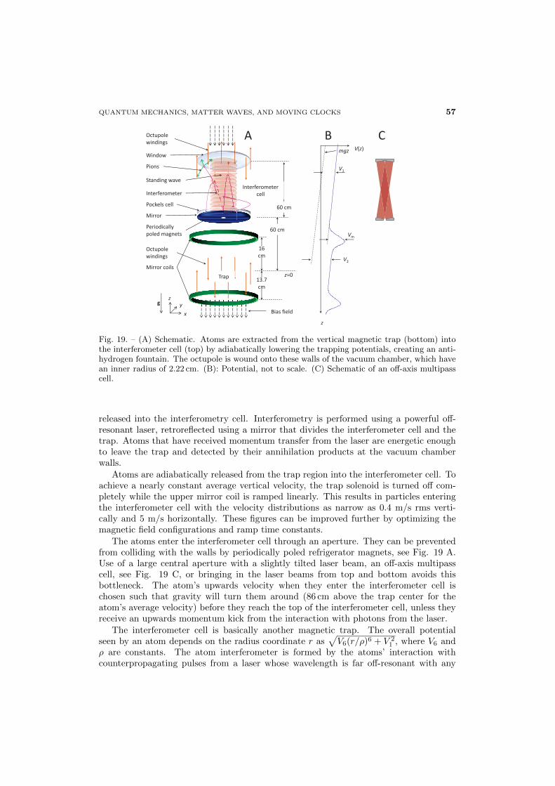
QUANTUM MECHANICS, MATTER WAVES, AND MOVING CLOCKS 57
V(z)
z
mgz
V1
V2
Vm
Interferometer
Standing wave
Pions
x
y z
g
Mirror coils
Octupole windings
Window
Bias field
Mirror
z=0 13.7 cm
16 cm
60 cm
Octupole windings
60 cm
Trap
Interferometer cell
Pockels cell
Periodically poled magnets
A B C
Fig. 19. – (A) Schematic. Atoms are extracted from the vertical magnetic trap (bottom) intothe interferometer cell (top) by adiabatically lowering the trapping potentials, creating an anti-hydrogen fountain. The octupole is wound onto these walls of the vacuum chamber, which havean inner radius of 2.22 cm. (B): Potential, not to scale. (C) Schematic of an off-axis multipasscell.
released into the interferometry cell. Interferometry is performed using a powerful off-resonant laser, retroreflected using a mirror that divides the interferometer cell and thetrap. Atoms that have received momentum transfer from the laser are energetic enoughto leave the trap and detected by their annihilation products at the vacuum chamberwalls.
Atoms are adiabatically released from the trap region into the interferometer cell. Toachieve a nearly constant average vertical velocity, the trap solenoid is turned off com-pletely while the upper mirror coil is ramped linearly. This results in particles enteringthe interferometer cell with the velocity distributions as narrow as 0.4 m/s rms verti-cally and 5 m/s horizontally. These figures can be improved further by optimizing themagnetic field configurations and ramp time constants.
The atoms enter the interferometer cell through an aperture. They can be preventedfrom colliding with the walls by periodically poled refrigerator magnets, see Fig. 19 A.Use of a large central aperture with a slightly tilted laser beam, an off-axis multipasscell, see Fig. 19 C, or bringing in the laser beams from top and bottom avoids thisbottleneck. The atom’s upwards velocity when they enter the interferometer cell ischosen such that gravity will turn them around (86 cm above the trap center for theatom’s average velocity) before they reach the top of the interferometer cell, unless theyreceive an upwards momentum kick from the interaction with photons from the laser.
The interferometer cell is basically another magnetic trap. The overall potentialseen by an atom depends on the radius coordinate r as
√V6(r/ρ)6 + V 2
1 , where V6 andρ are constants. The atom interferometer is formed by the atoms’ interaction withcounterpropagating pulses from a laser whose wavelength is far off-resonant with any
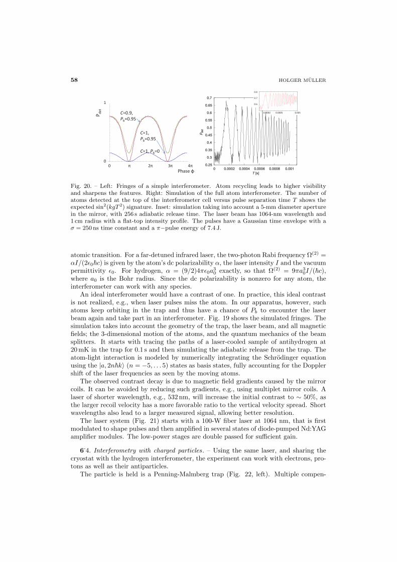
58 HOLGER MULLER
C=0.9, Pb=0.95
C=1, Pb=0.95
C=1, Pb=0
0 π 2π 3π 4π Phase φ
1 0
P det
0.0002 0.0005 0.001
0.8 0.7 0.6
Fig. 20. – Left: Fringes of a simple interferometer. Atom recycling leads to higher visibilityand sharpens the features. Right: Simulation of the full atom interferometer. The number ofatoms detected at the top of the interferometer cell versus pulse separation time T shows theexpected sin2(kgT 2) signature. Inset: simulation taking into account a 5-mm diameter aperturein the mirror, with 256 s adiabatic release time. The laser beam has 1064-nm wavelength and1 cm radius with a flat-top intensity profile. The pulses have a Gaussian time envelope with aσ = 250 ns time constant and a π−pulse energy of 7.4 J.
atomic transition. For a far-detuned infrared laser, the two-photon Rabi frequency Ω(2) =αI/(2ε0~c) is given by the atom’s dc polarizability α, the laser intensity I and the vacuumpermittivity ε0. For hydrogen, α = (9/2)4πε0a
30 exactly, so that Ω(2) = 9πa3
0I/(~c),where a0 is the Bohr radius. Since the dc polarizability is nonzero for any atom, theinterferometer can work with any species.
An ideal interferometer would have a contrast of one. In practice, this ideal contrastis not realized, e.g., when laser pulses miss the atom. In our apparatus, however, suchatoms keep orbiting in the trap and thus have a chance of Pb to encounter the laserbeam again and take part in an interferometer. Fig. 19 shows the simulated fringes. Thesimulation takes into account the geometry of the trap, the laser beam, and all magneticfields; the 3-dimensional motion of the atoms, and the quantum mechanics of the beamsplitters. It starts with tracing the paths of a laser-cooled sample of antihydrogen at20 mK in the trap for 0.1 s and then simulating the adiabatic release from the trap. Theatom-light interaction is modeled by numerically integrating the Schrodinger equationusing the |a, 2n~k〉 (n = −5, . . . 5) states as basis states, fully accounting for the Dopplershift of the laser frequencies as seen by the moving atoms.
The observed contrast decay is due to magnetic field gradients caused by the mirrorcoils. It can be avoided by reducing such gradients, e.g., using multiplet mirror coils. Alaser of shorter wavelength, e.g., 532 nm, will increase the initial contrast to ∼ 50%, asthe larger recoil velocity has a more favorable ratio to the vertical velocity spread. Shortwavelengths also lead to a larger measured signal, allowing better resolution.
The laser system (Fig. 21) starts with a 100-W fiber laser at 1064 nm, that is firstmodulated to shape pulses and then amplified in several states of diode-pumped Nd:YAGamplifier modules. The low-power stages are double passed for sufficient gain.
6.4. Interferometry with charged particles. – Using the same laser, and sharing the
cryostat with the hydrogen interferometer, the experiment can work with electrons, pro-tons as well as their antiparticles.
The particle is held is a Penning-Malmberg trap (Fig. 22, left). Multiple compen-
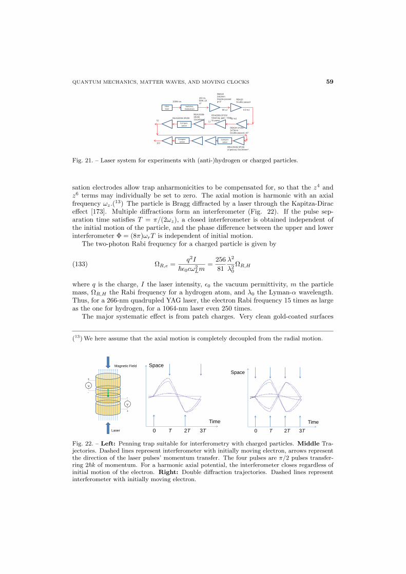
QUANTUM MECHANICS, MATTER WAVES, AND MOVING CLOCKS 59
Fiber laser
100W cw
Switches, modulators
200 ns, 50W, 10 uJ
REA15008-3P200 (4 pieces) 15x146mm2
REA10008-3P200 10x146mm2
REA6308-2P200 Small sig. gain ~30@ 3J pump
RBA34-1P200 3x73mm Double-passed, x62
RBA20 2x63mm Double passed g=32
REA10008-3P200
RBA20 Double passed
5J 1J 30 mJ
90 uJ 0.8 mJ
10J
Compen-sation
Compen-sation
Compen-sation
Fig. 21. – Laser system for experiments with (anti-)hydrogen or charged particles.
sation electrodes allow trap anharmonicities to be compensated for, so that the z4 andz6 terms may individually be set to zero. The axial motion is harmonic with an axialfrequency ωz.(
13) The particle is Bragg diffracted by a laser through the Kapitza-Diraceffect [173]. Multiple diffractions form an interferometer (Fig. 22). If the pulse sep-aration time satisfies T = π/(2ωz), a closed interferometer is obtained independent ofthe initial motion of the particle, and the phase difference between the upper and lowerinterferometer Φ = (8π)ωrT is independent of initial motion.
The two-photon Rabi frequency for a charged particle is given by
(133) ΩR,e =q2I
~ε0cω2Lm
=256
81
λ2
λ20
ΩR,H
where q is the charge, I the laser intensity, ε0 the vacuum permittivity, m the particlemass, ΩR,H the Rabi frequency for a hydrogen atom, and λ0 the Lyman-α wavelength.Thus, for a 266-nm quadrupled YAG laser, the electron Rabi frequency 15 times as largeas the one for hydrogen, for a 1064-nm laser even 250 times.
The major systematic effect is from patch charges. Very clean gold-coated surfaces
(13) We here assume that the axial motion is completely decoupled from the radial motion.
Laser
Magnetic Field
V
V
+
-
-
+
0 T 2T 3T
Time
Space
0 T 2T 3T
Time
Space
Fig. 22. – Left: Penning trap suitable for interferometry with charged particles. Middle Tra-jectories. Dashed lines represent interferometer with initially moving electron, arrows representthe direction of the laser pulses’ momentum transfer. The four pulses are π/2 pulses transfer-ring 2~k of momentum. For a harmonic axial potential, the interferometer closes regardless ofinitial motion of the electron. Right: Double diffraction trajectories. Dashed lines representinterferometer with initially moving electron.
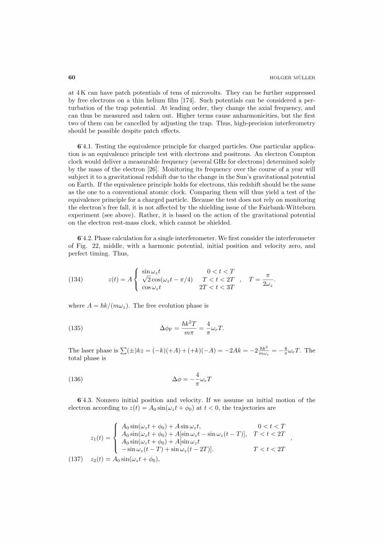
60 HOLGER MULLER
at 4 K can have patch potentials of tens of microvolts. They can be further suppressedby free electrons on a thin helium film [174]. Such potentials can be considered a per-turbation of the trap potential. At leading order, they change the axial frequency, andcan thus be measured and taken out. Higher terms cause anharmonicities, but the firsttwo of them can be cancelled by adjusting the trap. Thus, high-precision interferometryshould be possible despite patch effects.
6.4.1. Testing the equivalence principle for charged particles. One particular applica-
tion is an equivalence principle test with electrons and positrons. An electron Comptonclock would deliver a measurable frequency (several GHz for electrons) determined solelyby the mass of the electron [26]. Monitoring its frequency over the course of a year willsubject it to a gravitational redshift due to the change in the Sun’s gravitational potentialon Earth. If the equivalence principle holds for electrons, this redshift should be the sameas the one to a conventional atomic clock. Comparing them will thus yield a test of theequivalence principle for a charged particle. Because the test does not rely on monitoringthe electron’s free fall, it is not affected by the shielding issue of the Fairbank-Wittebornexperiment (see above). Rather, it is based on the action of the gravitational potentialon the electron rest-mass clock, which cannot be shielded.
6.4.2. Phase calculation for a single interferometer. We first consider the interferometer
of Fig. 22, middle, with a harmonic potential, initial position and velocity zero, andperfect timing. Thus,
(134) z(t) = A
sinωzt 0 < t < T√
2 cos(ωzt− π/4) T < t < 2Tcosωzt 2T < t < 3T
, T =π
2ωz.
where A = ~k/(mωz). The free evolution phase is
(135) ∆φF =~k2T
mπ=
4
πωrT.
The laser phase is∑
(±)kz = (−k)(+A) + (+k)(−A) = −2Ak = −2 ~k2mωz
= − 8πωrT . The
total phase is
(136) ∆φ = − 4
πωrT
6.4.3. Nonzero initial position and velocity. If we assume an initial motion of the
electron according to z(t) = A0 sin(ωzt+ φ0) at t < 0, the trajectories are
z1(t) =
A0 sin(ωzt+ φ0) +A sinωzt, 0 < t < TA0 sin(ωzt+ φ0) +A[sinωzt− sinωz(t− T )], T < t < 2TA0 sin(ωzt+ φ0) +A[sinωzt− sinωz(t− T ) + sinωz(t− 2T )]. T < t < 2T
,
z2(t) = A0 sin(ωzt+ φ0),(137)
QUANTUM MECHANICS, MATTER WAVES, AND MOVING CLOCKS 61
where A = ~k/(mωz) and A0 = ~k0/(mωz). For T = π/(2ωz), the interferometer closesfor all A0, φ0. We calculate the free evolution phase as
∆φF =ωrωz
[3 cosωzT − 4 cos 2ωzT − 2 cos 4ωzT + cos 5ωzT +
k0
k(2 cos(ωzT + φ0)
−2 cos(2ωzT + φ0) + 4 cos(3ωzT + φ0)− 2 cos(4ωzT + φ0) + 2 cos(5ωzT + φ0))] sinωzT.
Proceeding as above, we calculate the total phase. In order to study the effect of slighttiming errors or uncertainty in omegaz, we substitute ωz → ωz + δz, where δz is small.
∆φ =4
πωrT
(1− k0
k(cosφ0 − sinφ0)
)− 4
π2ωrδzT
2 2(π − 1)
+k0
k[2(π + 1) cosφ0 + (π − 2) sinφ0]
(138)
In principle one could scan T and zero the δ−dependent term.
6.4.4. Double diffraction. Since the above methods are sensitive to the atom’s initial
oscillation, we’ll try a more complicated scheme with double diffraction, i.e., two interfer-ometers in which the recoil directions are reversed relative to each other. The trajectoriesof the first interferometer are given by Eq. (137), the third trajectory is
(139) z3(t) =
A0 sin(ωzt+ φ0)−A sinωzt, 0 < t < TA0 sin(ωzt+ φ0)−A[sinωzt− sinωz(t− T )], T < t < 2TA0 sin(ωzt+ φ0)−A[sinωzt− sinωz(t− T ) + sinωz(t− 2T )]. T < t < 2T
Each interferometer has a phase ∆φA = ∆φAF + ∆φAI ,∆φB = ∆φBF + ∆φBI . Their sum,
Φ = ∆φA + ∆φB(140)
= 2ωrωz
sin 12ωzT
(3 cos 1
2ωzT − cos 32ωzT + 2 cos 7
2ωzT − cos 92ωzT + cos 11
2 ωzT)
is completely independent of initial electron motion. We let ωz = π/(2T )+δz and expand
(141) Φ =8
πωrT +
16
π2(π − 1)T 2δz +
4
π3ωrT
3δ2z(8− 8π + 7π2) + ...
6.4.5. Trap anharmonicity. Let’s say the trap potential is
(142) V =1
2mω2
zd2
(z2
d2+D3
z3
d3+D4
z4
d4+ . . .
),
where d is the typical trap size and D3,4,... are coefficients. We assume the anharmonicityis low so it can be treated perturbatively, integrating the anharmonic parts over the
62 HOLGER MULLER
unperturbed trajectories. The result is a shift
∆Φ = 8ω2rT
2
k2π3r2[4D3k0πd(cosφ0 − sinφ0)(143)
+D4ωrT (9π − 16 + 24k2
0
k2(π − 1) + 6
k20
k2π sin 2φ0)]
which is zero if there is no initial motion, k0 = 0. For ωr = 2π × 1.2 GHz, T = 2.8 ms,k = 2× 2π/1064 nm, and r = 2 cm, we obtain
(144)∆Φ
Φ0= −1.7× 10⁻⁹D3
k0
m−1(sinφ0 − cosφ0) + 3.2× 10⁻⁴D4
where we have neglected terms proportional to k20. The coefficient D4 can be of order
10−4 and D3 is expected to be much lower for symmetry reasons, so we expect the errordue to anharmonicity to be better than 32 ppb. That can be improved with a larger trap.
6.4.6. Non-closure of the interferometer. We treat the trajectory change perturba-
tively. Neglecting damping, the classical trajectory of the electron satisfies
(145) zi(t) + ω2z(t)z = Fi(t)/m
Using a Green’s function G(t, t′) = 1/(mωz) sinωz(t−t′), the resulting displacement δi(t)of the trajectory zi at time t is given by
(146) δi(t) =1
mωz
∫ t
−∞Fi(t
′) sinωz(t− t′)dt.
The force is due to the z4i term in the potential, Fi(t) = 2mω2
zD4z3i (t)/d2 with zi(t)
given by Eqs. (137,139), respectively, for the three trajectories. In particular, we areinterested in δi ≡ δi(3T ), i.e., the displacement of the wave packets when they interfereat t = 3T . We find a gap between z1 and z2 of
(147) δ1(3T )− δ2(3T ) =32√
2D4v2rv0T
3
d2π3sin(φ0 − π/4) +O(k2
0),
where we assume ωz = π/(2T ) and neglected terms quadratic in v0 = ~k0/m. The othergap δ2(3T ) − δ3(3T ) = −δ1(3T ) + δ2(3T ) (to leading order) is calculated in a similarmanner. If the electrons have a temperature Te, we may insert the average electronvelocity v0 =
√kBTe/m. Comparing the gap with the thermal de Broglie wavelength
h/√
2πmkBTe gives an upper limit on the electron temperature Te of
(148)hdπ5/2
64D4v2rT
3kB= Te.
For the design parameters of Tab. X, this amounts to 15 mK, doable in a dilutionrefrigerator.
QUANTUM MECHANICS, MATTER WAVES, AND MOVING CLOCKS 63
Table X. – Numerical example for an electron interferometer
Parameter value
Laser wavelength λ 1064 nmEffective wavenumber k 1.2× 10⁷/m
Recoil frequency ωr 2π × 1.2 GHzRecoil temperature 57 mK
Axial frequency ωz 2π × 10 kHzAxial amplitude A 2.1 cmTypical trap size d 10 cm
Axial loss resistance R 10 kΩAxial damping (κ ∼ 1 characterizes trap geometry) γ = (eκ/2d)2R/m 2π × 0.7 mHz
Pulse separation times T = π/(2ωz) 25µsPhase Φ0 = 8ωrT/π 5.1× 10⁵ rad
6.4.7. Decoherence from axial damping. Axial motion in the Penning trap is damped
with a decay rate of γ, proportional to a loss resistance R, but independent of ωz. Theresistance R is usually made as large as technically feasible, as this facilitates electrondetection. For R ∼ 105 Ω, we obtain γ ∼ 2π×10 Hz for a normal-sized trap. By choosingR as low as possible, we can get γ to, let’s say, 2π × 1µHz.
The decay rate for the sth harmonic oscillator state is sγ and limits the coherencetime of the interferometer. Since s ' ωr/ωz (the electrons are not in a pure HO quantumstate), the coherence time is limited to τ ≈ ωz/(ωrγ), and for reasonable interferencecontrast, we need 4T < τ . Let’s say we are working at 4T = τ . The phase Φ of theinterferometer is thus limited to 2
πωrωzωrγ
= 2πωzγ = 2
πQ, where Q = ωz/γ is the quality
factor of the axial motion. Since T = τ/4 = ωz/(4ωrγ) and ωz = π/(2T ), we obtainT = π
8Tωrγ, we get the following combination of parameters that lead to optimum phase
Φopt:
(149) T =√π/(8ωrγ), ωz =
π
2√π/(8ωrγ)
= 2√πωrγ, Φopt =
4
π
√πωrγ
γ= 4
√ωrπγ
For ωr = 2π × 1.2 GHz, γ = 2π × 1µHz, we obtain T = 2.8 ms, ωr = 2π × 122 Hz, andΦopt = 7.8× 10⁷.
6.4.8. Example. Table X gives a numerical example. Obviously, many questions re-
main to be addressed, such as how to cool electrons. Given that we can use only oneelectron at a time, how can we repeat the experiment rapidly so as to obtain good statis-tics? This will probably require nondestructive detection of the electron. The purpose ofthese sections is not to answer all these questions, but to present the phase calculation,showing that high-precision electron interferometry is, in principle, possible, and whatthe challenges are.
7. – Interferometry in space
7.1. Concept . – Operation in space offers a number of potential advantages. Experi-
ments can use long interrogation times due to absence of free fall of the atoms relative tothe apparatus, the possibility to suppress systematic effects by inverting the experiment
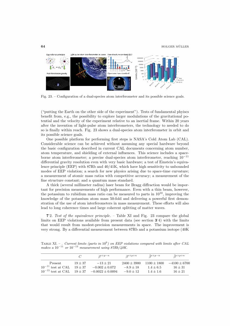
64 HOLGER MULLER
Now CAL 10-11
CAL 10-13
1
10
100
1000
10000
100000
1000000
10000000
Lim
its (1
0-12 )
Fig. 23. – Configuration of a dual-species atom interferometer and its possible science goals.
(“putting the Earth on the other side of the experiment”). Tests of fundamental phyiscsbenefit from, e.g., the possibility to explore larger modulations of the gravitational po-tential and the velocity of the experiment relative to an inertial frame. Within 20 yearsafter the invention of light-pulse atom interferometers, the technology to needed to doso is finally within reach. Fig. 23 shows a dual-species atom interferometer in orbit andits possible science goals.
One possible platform for performing first steps is NASA’s Cold Atom Lab (CAL).Considerable science can be achieved without assuming any special hardware beyondthe basic configuration described in current CAL documents concerning atom number,atom temperature, and shielding of external influences. This science includes a space-borne atom interferometer; a precise dual-species atom interferometer, reaching 10−11
differential gravity resolution even with very basic hardware; a test of Einstein’s equiva-lence principle (EEP) with 87Rb and 40/41K, which have high sensitivity to unboundedmodes of EEP violation; a search for new physics arising due to space-time curvature;a measurement of atomic mass ratios with competitive accuracy; a measurement of thefine structure constant; and a quantum mass standard.
A thick (several millimeter radius) laser beam for Bragg diffraction would be impor-tant for precision measurements of high performance. Even with a thin beam, however,the potassium to rubidium mass ratio can be measured to parts in 1010, improving theknowledge of the potassium atom mass 50-fold and delivering a powerful first demon-stration of the use of atom interferometers in mass measurement. These efforts will alsolead to long coherence times and large coherent splitting of matter waves.
7.2. Test of the equivalence principle. – Table XI and Fig. 23 compare the global
limits on EEP violations available from present data (see section 3.4) with the limits
that would result from modest-precision measurements in space. The improvement isvery strong. By a differential measurement between 87Rb and a potassium isotope (40K
Table XI. – . Current limits (parts in 109) on EEP violations compared with limits after CALmakes a 10−11 or 10−13 measurement using 87Rb/40K.
C βe+p−n βe+p+n βe+p−n βe+p+n
Present 19± 37 −13± 21 2400± 3900 1100± 1800 −4100± 670010−11 test at CAL 19± 37 −0.002± 0.072 −8.9± 18 1.4± 6.5 16± 3110−13 test at CAL 19± 37 −0.0022± 0.0094 −9.0± 12 1.4± 1.6 16± 21
QUANTUM MECHANICS, MATTER WAVES, AND MOVING CLOCKS 65
or 41K), the spaceborne experiment will measure a combination of coefficients that isconsiderably different from any combination measured before. Thus, even a modestlysensitive result can improve the global bounds on EEP violation for classical matter bya factor of 200-300 for four of the five coefficients.
7.2.1. Advantages of quantum tests of the EEP in space. Spaceborne atom inter-
ferometers are sensitive to modes in which the EEP might fail that are inaccessible toterrestrial or classical experiments. Compared to classical tests, they can operate withspin-polarized matter and thus place bounds on EEP violating effects that might coupleto the quantum properties of matter. Spin-dependent gravitational couplings have longbeen studied in the context of theories of gravity with nonvanishing torsion. A quan-tum tests of the EEP will perform the first or most sensitive measurement on severalbµ, dµν , g
µ, fµν , gλµν , and Hµν coefficients of the SME. In addition, they are sensitiveto the phase of the matter-wave packet, whereas classical tests sense only the centerof mass-motion. Schiff’s conjecture implies that information gained from this phase isequivalent to the one measured in classical tests. After 50 years, however, the conjec-ture has neither been proved nor disproved. Quantum tests of the EEP are tests of thegravitational redshift for matter waves and currently the most sensitive probes by far forrelativity violations outside of Schiff’s conjecture [2].
Compared to terrestrial tests, these experiments are sensitive to effects that mightarise at higher post-Newtonian order, PNO. Effects of gravity can be grouped by theirsuppression in powers of 1/c. Newtonian gravity enters the metric proportional to 1/c2
and are thus labelled PNO(2). Higher-order effects such as frame-dragging or perihelionprecession arise at PNO(3) and PNO(4), respectively. The large modulation of positionand velocity provided by the Space Station’s orbit helps detecting PNO(3) and PNO(4)-signals that might arise from the nonlinearity of general relativity. This enables a searchfor effects of higher-mass dimension operators of the SME, e.g., EEP violation thatscales with the velocity of the system. Such effects have never been the subject of directexperimental study, and could be extremely large, yet unnoticed so far.
7.3. Recoil measurements and mass standard . – By reprogramming, the spaceborne
atom interferometer can measure the recoil frequency ωr = ~k2/(2m) = ω2L/ωC of the
atoms. If ωL is known, this translates to a measurement of ~/m or equivalently theCompton frequency ωC of the atom.
7.3.1. Fine structure constant. Combined with the Rydberg constant Ry and the iso-
topes’ mass ratios m/me with the electron, this measurement can be used to determinethe fine structure constant α, see section 4
.6. The performance of CAL in such a mea-
surement will depend heavily on its design. A very basic CAL having a thin opticallattice beam will not reach beyond a 10−8 accuracy. This can be improved by precisecalibration of the lattice beam’s wavefronts, and/or by using a thicker beam. An inter-ferometer having a 2.5-mm beam waist beam could reach well beyond the ppb level andprovide the most precise measurement of h/m and the fine structure constant.
Comparison of α as measured by atom interferometers and by the electron’s gyromag-netic ratio g can yield the most precise test of QED and limit a possible inner structureof the electron. If g doesn’t deviate from the expected value by more than δg, the energyscale m∗ of such a substructure must be m∗ > me/(δg/2)1/2 in the chirally invariantmodel [182] (other models lead to a linear scaling and thus a larger scale). Current datayields m∗ > 0.7 GeV, limited by measurements of α. Data from the large electron-protoncollider sets a limit of 10 TeV; a space-borne measurement at 10−10 precision could reach
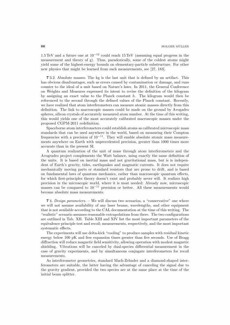
66 HOLGER MULLER
1.5 TeV and a future one at 10−12 could reach 15 TeV (assuming equal progress in themeasurement and theory of g). Thus, paradoxically, some of the coldest atoms mightyield some of the highest-energy bounds on elementary-particle substructure. For othernew physics that might be learned from such measurements, see [27, 183].
7.3.2. Absolute masses. The kg is the last unit that is defined by an artifact. This
has obvious disadvantages, such as errors caused by contamination or damage, and runscounter to the ideal of a unit based on Nature’s laws. In 2011, the General Conferenceon Weights and Measures expressed its intent to revise the definition of the kilogramby assigning an exact value to the Planck constant h. The kilogram would then bereferenced to the second through the defined values of the Planck constant. Recently,we have realized that atom interferometers can measure atomic masses directly from thisdefinition. The link to macroscopic masses could be made on the ground by Avogadrospheres, silicon crystals of accurately measured atom number. At the time of this writing,this would yields one of the most accurately calibrated macroscopic masses under theproposed CGPM-2011 redefinition.
Spaceborne atom interferometers could establish atoms as calibrated microscopic massstandards that can be used anywhere in the world, based on measuring their Comptonfrequencies with a precision of 10−11. They will enable absolute atomic mass measure-ments anywhere on Earth with unprecedented precision, greater than 1000 times moreaccurate than in the present SI.
A quantum realization of the unit of mass through atom interferometers and theAvogradro project complements the Watt balance, using exactly the same definition ofthe units. It is based on inertial mass and not gravitational mass, but is is indepen-dent of Earth’s gravity, tides, earthquakes and magmatic currents. It does not requiremechanically moving parts or standard resistors that are prone to drift, and is basedon fundamental laws of quantum mechanics, rather than macroscopic quantum effects,for which first-principles theory doesn’t exist and probably never will. It realizes highprecision in the microscopic world, where it is most needed: Already now, microscopicmasses can be compared to 10−11 precision or better. All these measurements wouldbecome absolute mass measurements.
7.4. Design parameters. – We will discuss two scenarios, a “conservative” one where
we will not assume availability of any laser beams, wavelengths, and other equipmentthat is not available according to the CAL documentation at the time of this writing. The“realistic” scenario assumes reasonable extrapolations from there. The two configurationsare outlined in Tab. XII. Table XIII and XIV list the most important parameters of theequivalence principle test and recoil; measurements, respectively, and the most importantsystematic effects.
The experiments will use delta-kick “cooling” to produce samples with residual kineticenergy below 100 pK and free expansion times greater than five seconds. Use of Braggdiffraction will reduce magnetic field sensitivity, allowing operation with modest magneticshielding. Vibrations will be canceled by dual-species differential measurement in thecase of gravity experiments, and by simultaneous conjugate interferometers for recoilmeasurements.
As interferometer geometries, standard Mach-Zehnder and a diamond-shaped inter-ferometers are suitable, the latter having the advantage of canceling the signal due tothe gravity gradient, provided the two species are at the same place at the time of theinitial beam splitter.
QUANTUM MECHANICS, MATTER WAVES, AND MOVING CLOCKS 67
Table XII. – . Dimensions of the conservative and realistic scenario
Conservative Realistic Remarks
Atom temperature 100 pK 100 pKAtom number (Rb/K) 104/104 2× 10⁵/105
Lattice wavelength 850 nm 850 or 676 nm 676 nm leads to same latticedepth for Rb and K
Lattice laser power 10-50 mW 0.1 W 2-3 recoil lattice depthLattice beam 1/e2 radius 0.5 mm 3 mm Limited by separation of
atoms from chipFree expansion time 5 s 5 s CAL documents suggest up
to 20 sTip-tilt mirror for lattice beam No YesRF reference stability 10−8 10−11 For recoil measurementMagnetic shielding factor 100 1000Vibrations Not critical Not critical
Table XIII. – Equivalence principle tests in space using CAL. Note that the “conservative”experiment does not assume a pulse separation time any longer than what is now routine inthe lab. Taking advantage of microgravity allows the realistic scenario to gain much betterperformance. A EEP test at 10−11 sensitivity is easily compatible with the estimated systematiceffects, leaving considerable room for tradeoffs with other projects at CAL.
Parameter Conservative Realistic
Pulse separation time 0.5 s 2 sMomentum transfer 2~k 2~kGravity phase [rad] 1.8× 10⁷ 3× 10⁸
Differential resolution δg/g (1 day) 1× 10⁻¹¹ 1.5× 10⁻¹³
Magnetic field systematic 3× 10⁻¹¹ 1.5× 10⁻¹³
Gravity gradient influence due to initial cloud mis-match as caused by magnetic fields
1.4× 10⁻¹¹g 1.4× 10⁻¹³g
Table XIV. – Recoil measurement at CAL. These experiments require the realistic scenario tosurpass the precision attained in terrestrial experiments, but even the conservative scenario willlead to a 50-fold improvement in the Potassium mass.
Parameter Conservative Realistic
Pulse separation time 0.5 s 0.5 sMomentum transfer 2~k 4~kRecoil phase [rad] 4× 10⁴ 3× 10⁵
Differential resolution (1 day) 5× 10⁻⁹ 1.5× 10⁻¹⁰
Magnetic field systematic 3× 10⁻¹⁰ 1.5× 10⁻¹¹
Gravity gradient (known to 10−3) (150± 0.15)× 10−9 (1500± 1.5)× 10−10
Beam splitter phase 1.4× 10⁻¹⁰ 1.4× 10⁻¹⁰
Guoy phase, wavefront curvature (charac-terized to 1%)
(3± 0.03)× 10−7 (8± 0.1)× 10−9
RF reference uncertainty 10−8 10−11
Total systematic error + noise 1.1× 10⁻⁸ 3× 10⁻¹⁰
68 HOLGER MULLER
7.5. Inversion of the setup. – Higher-precision experiments that are possible in a
dedicated mission will most likely be limited by the gravity gradient, which causes aparasitic signal if the overlap of the two species is not perfect. It takes an overlapaccuracy of nanometers to reach a precision in the 10−15 range in an EEP tests. Inspace, however, it is possible to invert the setup on a gimbal, thus “putting the Earth onthe other side of the experiment.” This will help to greatly suppress systematic effects.
8. – Summary and outlook
The snapshot of atom interferometry presented in this paper is by no means complete.However, we hope to have shown that the field is interesting from both the point of viewof fundamental physics and applications. On the fundamental side, it inspired takinga new look at de Broglie’s view that matter-wave packets are like oscillators (“clocks”)ticking at an incredibly high frequency. We showed that this concept is powerful enoughto derive all equations of motion of quantum mechanics, by contrast to what has beenthought before. We hope that the concept might prove fruitful in the further developmentof quantum theory, e.g., for directly obtaining a theory of fermions from the Nambu-Gotoaction [147] in string theory. It might reveal new effects, such as gravitational Aharonov-Bohm effects described by the Dirac equation in curved space-time.
Might relativistic effects be observable in electron interferometers? Such effects shouldscale like (nωL/ωC)2, where n is the number of photon momenta transferred by the laserand ωC/(2π) ∼ 1.1× 10²⁰ Hz is the electron’s Compton frequency. For a laser frequencyωL corresponding to a wavelength of 266 nm, this amounts to 4× 10⁻¹⁰; measurement isnot completely out of the question. Such relativistic effects could include a dependence ofthe interferometer phase on the relative orientation of spin and momentum (“spin-orbitcoupling”). Observation of spin-gravity coupling would be even more exciting. In anelectron interferometer (similar to Fig. 22) with a pulse separation time of T , the phaseinduced by spin-gravity coupling will be ∼ (ωL/ωC)2nkgT 2 ∼ 2× 10⁻⁷ rad for the aboveparameters and T = 1 ms. The splitting of the electron trajectories in such a devicewould amount to 6 meters; maybe the high velocities can be contained in the cyclotronmotion in the trap.
In experiments, we have tested the equivalence principle and other properties of grav-ity, in particular the gravitational redshift and the isotropy of gravity. We obtainedcomprehensive bounds on equivalence-principle violations in the standard model exten-sion (SME). These limits are comprehensive: No experiment may evade them unless oneassumes physics beyond the SME, such as violation of energy-momentum conservationor the existence of additional matter fields or forces. Nevertheless, in a universe in whichwe cannot explain the observed dominance of matter over antimatter, or account for95% of the observed mass-energy, it would be presumptuous to categorically rule out anypossibility of equivalence principle violations not described by the SME.
Atom interferometry has already now achieved the accuracy needed to play a signifi-cant part in the measurement of microscopic masses in the future redefinition of the inter-national system of units. While measurement of macroscopic masses will rarely be moreprecise than a few parts in 109 (due, e.g., to contamination and outgassing), microscopicmasses can already now be compared to parts in 1011. With better Compton-frequencymass standards, all these relative measurements will become absolute. Macroscopic stan-dards can be derived from microscopic ones by Avogradro spheres, which at the time ofthis writing have an accuracy of 30 ppb. They are expected to improve in the future.
Finally, we hope to have given a glimpse of prospects for interferometry with new
QUANTUM MECHANICS, MATTER WAVES, AND MOVING CLOCKS 69
types of particles, such as antimatter or charged (anti-)particles, and the new types ofexperiments enabled by them, such as equivalence principle tests with charged particles.
Many other ideas are currently pursued by researchers world-wide, e.g., gravitationalwave detection, compact atom interferometers, navigation and geophysics, gravity gradi-ent measurements, or single-atom interferometry, to name just a few. The field of atominterferometry has a bright future.
∗ ∗ ∗I would like to acknowledge the support of the National Science Foundation, the
National Aeronautics and Space Agency, the David and Lucile Packard Foundation, theAlfred P. Sloan Foundation, and Lawrence Berkeley National Lab.
Many thanks to Paul Hamilton for his very careful and insightful reading of themanuscript. I have the privilege to work with a number of great scientists and amgrateful to all of them, in particular all members of my group at Berkeley since 2009. Iwould like to highlight those involved directly with the work reported here: Justin Brown,Steven Chu, Brian Estey, Joel Fajans, Ori Ganor, Paul Hamilton, Mike Hohensee, SabineHossenfelder, Matt Jaffe, Pei-Chen Kuan, Alan Kostelecky, Shau-Yu Lan, Jay Tasson,Bob Wiringa, Jonathan Wurtele, Chenghui Yu, Nan Yu, Anton Zeilinger, and AndreiZhmoginov. Thanks to Guglielmo Tino and Mark Kasevich for the invitation to theSummer School. I thoroughly enjoyed the science and friendship experienced there.Finally, thanks to my family for their patience.
REFERENCES
[1] L. de Broglie, “Recherches sur la theorie des Quanta” (Ph. D. thesis, Univ. Paris 1924).[2] H. Muller, A. Peters, and S. Chu, Nature 463, 926 (2010); ibid. 467, E2 (2010).[3] M. A. Hohensee, S. Chu, A. Peters, and H. Muller, Phys. Rev. Lett. 106, 151102 (2011).[4] A. M. Nobili et al., Am. J. Phys. 81, 527-536 (2013).[5] Y. Bonder et al. Phys. Rev. D 87, 125021 (2013).[6] A. G. Klein, Physica Scripta T153 014038 (2013).[7] J. Lindesay, Found. Phys. 42, 1573-1585 (2012).[8] S. Hacyan, Phys. Rev. D 85 024035 (2012).[9] C. T. Ridgely et al., Ann. Phys. (Berlin) 523, 805-812 (2011).[10] C. T. Ridgley, Eur. J. Phys. 31, 949-960 (2010).[11] S. Carloni, D. Grunmiller, and F. Preis, Phys. Rev. D 83, 124024 (2011).[12] C. W. Chou et al., Science 329, 1630-1633 (2010).[13] N. Poli et al., Phys. Rev. Lett. 106, 038501 (2011).[14] B. Berrett et al., in: E. Arimondo, P. R. Berman, and C. C. Lin, Advances in Atomic,
Molecular, and Optical Physics 60, 119-199 (2011).[15] L. Zhou et al., Chinese Phys. Lett. 28, 013701 (2012).[16] M. A. Hohensee and H. Muller, J. Mod. Opt. 58, 2021-2027 (2011).[17] A. Hakimov et al., Mod. Phys. Lett. A 25, 3115-3127 (2010).[18] F. Sorrentino et al., New J. Phys. 12, 095009 (2010).[19] E. Kajari, N. L. Harshman, E. M. Rasel, S. Stenholm, G. Suessmann, and W. P. Schleich,
Appl. Phys. B 100 43-60 (2010).[20] A. Alberti et al., New J. Phys. 12, 065037 (2010).[21] H. Abele and H. Leeb, New J. Phys. 14, 055010 (2012).[22] M. A. Hohensee et al., Phys. Rev. Lett. 108, 230404 (2012).[23] D. Dolce, Eur. Phys. Lett. 102, 31002 (2013).[24] A. Bassi et al., Rev. Mod. Phys. 85, 471-527 (2013).[25] M. P. Blencowe, Phys. Rev. Lett. 111, 021302 (2013).
70 HOLGER MULLER
[26] S.-Y. Lan et al., Science 339, 554 (2013).[27] H. Muller, S.-w. Chiow, Q. Long, C. Vo, and S. Chu, Appl. Phys. B 84, 633-642 (2006).[28] S.-w. Chiow, S. Herrmann, H. Muller, and S. Chu, Optics Express 17, 5246 (2009).[29] R. Bouchendira, P. Clade, S. Guellati-Khelifa, F. Nez, and F. Biraben, Phys. Rev. Lett.
106, 080801 (2011).[30] R. Bouchendira et al., Ann. Phys. (Berlin) 525, 484-92 (2013).[31] M. Zych et al. Class. Quantum Gravity 29, 224010 (2012).[32] M. Zych et al., Nature Comm. 2, 505 (2011).[33] S. Dimopoulos, P. W. Graham, J. M. Hogan, and M. A. Kasevich, Phys. Rev. D 78, 042003
(2008).[34] P. W. Graham, J. M. Hogan, M. A. Kasevich, S. Rajendran, arXiv:1206.0818; S.
Dimopoulos, P. W. Graham, J. M. Hogan, M. A. Kasevich, S. Rajendran, Phys. Rev. D 78,122002 (2008).
[35] J. M. Hogan et al., Gen. Relativity Gravitat. 43, 1953-2009 (2011).[36] P. W. Graham, J. M. Hogan, M. A. Kasevich, and Surjeet Rajendran Phys. Rev. Lett.
110, 171102 (2013).[37] P. Wolf et al., Nature 467, E1 (2010); H. Muller, A. Peters, and S. Chu, Nature 467, E2
(2010).[38] M. A. Hohensee et al., Class. Quantum Gravity 29, 048001 (2012); P. Wolf et al., Class.
Quantum Gravity 29, xxxxxx (2012).[39] P. Wolf et al., Class. Quantum Gravity 28, 145017 (2011).[40] S. Sinha and J. Samuel, Class. Quantum Gravity 28, 145018 (2011).[41] D. Giulini, in F. Finster et al., Quantum Field and Gravity, Springer Basel AG 2012, pp
345-370[42] W. P. Schleich, D. M. Greenberger, and E. M. Rasel, New J. Phys. 15, 013007 (2013).[43] W. P. Schleich, D. M. Greenberger, and E. M. Rasel, Phys. Rev. Lett. 110, 010401 (2013).[44] D. M. Greenberger, W. P. Schleich, and E. M. Rasel, Phys. Rev. A 86, 063622 (2012).[45] M.-T. Jaekel, B. Lamine, and S. Reynaud, Class. Quantum Gravity 30, 065006 (2013).[46] R. P. Feynman, Rev. Mod. Phys. 20, 367-387 (1948).[47] R.P. Feynman, The Development of the Space-Time View of Quantum Electrodynamics.
In: Nobel Lectures, Physics 1963-1970 (Elsevier, Amsterdam, The Netherlands) 1972[48] T. Jacobson, Feynman’s checkerboard and other games. Lect. Notes Phys. 226, 386 (1985).[49] N.D. Birell and P.C.W. Davies, Quantum fields in curved space (Cambridge University
Press, Cambridge, England 1982).[50] Mayeul Arminjon and Frank Reifler, Equivalent forms of Dirac equations in curved
spacetimes and generalized de Broglie relations. E-print: arXiv:1103.3201v4 (2013).[51] See, e.g., J. Polchinski, String Theory Volume 1, An Introduction to the Bosonic String
(Cambridge University Press, Cambridge, England 1998).[52] D. Lust and S. Theisen, Lectures on String Theory (Springer, Berlin, Germany 1989), Eq.
(7.5)[53] A. D. Cronin, J. Schmiedmayer, and D. E. Pritchard, Rev. Mod. Phys. 81, 10511129 (2009).[54] A. Peters, K.-Y. Chung, and S. Chu, Nature 400, 849 (1999)[55] A. Peters, K.-Y. Chung, and S. Chu, Metrologia 38, 25-61 (2001).[56] Alan Kostelecky, Neil Russell, Data Tables for Lorentz and CPT Violation, Rev. Mod.
Phys. 83, 11 (2011), updated at arXiv:0801.0287[57] C.W. Misner, K.S. Thorne, and J.A. Wheeler, Gravitation (Freeman, San Francisco, 1970).[58] T. Damour, F. Piazza, and G. Veneziano, Phys. Rev. Lett. 89, 081601 (2002).[59] C.M. Will, Living Rev. Relativity 9, (2006)[60] C.M. Will, Theory and experiment in gravitational physics, (Cambridge University Press,
Cambridge, England, 1993).[61] R.F.C. Vessot, M.W. Levine, E.M. Mattison, E.L. Blomberg, T.E. Hoffman, G.U. Nystrom,
B.F. Farrel, R. Decher, P.B. Eby, C.R. Baugher, J.W. Watts, D.L. Teuber, and F.D. Wills,Phys. Rev. Lett. 45, 20812084 (1980).
[62] S. Schlamminger et al., Phys. Rev. Lett. 100, 041101 (2008); E.G. Adelberger at el., Prog.Particle and Nuclear Phys. 62, 102 (2009).
QUANTUM MECHANICS, MATTER WAVES, AND MOVING CLOCKS 71
[63] T.F. Damour and J.F. Donoghue, Phys. Rev. D 82, 084033 (2010).[64] D. Colladay and V.A. Kostelecky, Phys. Rev. D 55, 6760 (1997); ibid. 58, 116002 (1998).[65] V. A. Kostelecky, Phys. Rev. D 69, 105009 (2004)[66] V. A. Kostelecky and J. D. Tasson, Phys. Rev. Lett. 102, 010402 (2009).[67] V. A. Kostelecky and J. D. Tasson, Phys. Rev. D 83, 016013 (2011).[68] Michael A. Hohensee, Holger Mller, and R. B. Wiringa, Phys. Rev. Lett. 111, 151102
(2013).[69] V.A. Kostelecky and M. Mewes, Phys. Rev. D 66, 056005 (2002)[70] Q.G. Bailey and V.A. Kostelecky, Phys. Rev. D 74, 045001 (2006).[71] V.A. Kostelecky and M. Mewes, Phys. Rev. Lett. 97, 140401 (2006); ibid. 99, 011601
(2007).[72] H. Muller et al., Phys. Rev. Lett. 100, 031101 (2008).[73] K.-Y. Chung et al., Phys. Rev. D 80, 016002 (2009).[74] C.M. Will, Astrophys. J. 169, 141 (1971); Living Rev. Rel. 4, 4 (2001).[75] Calculated from the Tamura [175] potentials using the ETGTAB v3.0 solid earth
tide data generation software by H.G. Wenzel, Univ. Karlsruhe. See, for example,http://www.geo.uni-jena.de/geophysik/etc/etcdat/etgtab/.
[76] G.D. Egbert, A. Bennett, and M.G.G. Foreman, J. Geophys. Res. 99, 24821 (1994).[77] J.B.R. Battat, J.F. Chandler, and C.W. Stubbs, Phys. Rev. Lett. 99, 241103 (2007).[78] J. H. Gundlach, S. Schlamminger, and T. A. Wagner, Space Sci. Rev. 148, 201 (2009).[79] N. Ashby et al., Phys. Rev. Lett. 98, 070802 (2007).[80] S. Blatt et al., Phys. Rev. Lett. 100, 140801 (2008).[81] T. M. Fortier et al., Phys. Rev. Lett. 98, 070801 (2007).[82] R.V. Pound and G.A. Rebka Jr., Phys. Rev. Lett. 4, 337 (1960); R.V. Pound and J.L.
Snider, Phys. Rev. Lett. 13, 539 (1964); Phys. Rev. 140, B788 (1965).[83] P. Clade et al., Europhys. Lett. 71, 730 (2005).[84] S. Schlamminger, K.-Y. Choi, T.A. Wagner, J.H. Gundlach, and E.G. Adelberger, Phys.
Rev. Lett. 100, 041101 (2008); J.H. Gundlach, S. Schlamminger, and T.A. Wagner, SpaceSci. Rev. 148, 201 (2009); Y. Su et al., Phys. Rev. D 50, 3614 (1994).
[85] N. Poli et al., Phys. Rev. Lett. 106, 038501 (2011); P. Clade et al., Europhys. Lett. 71,730 (2005); S. Merlet et al., Metrologia 47, L9 (2010).
[86] T. Damour, Class. Quant. Grav. 13, A33 (1996).[87] M.A. Hohensee, N. Leefer, D. Budker, C. Harabati, V.A. Dzuba, and V.V. Flambaum,
Phys. Rev. Lett. 111, 050401 (2013).[88] V.A. Kostelecky and J.D. Tasson, Phys. Rev. Lett. 102, 010402 (2009).[89] M.A. Hohensee and H. Muller, J. Mod. Opt. 58, 2021 (2011).[90] C.M. Will, Liv. Rev. Relativity 9, 3 (2006).[91] R.D. Woods and D.S. Saxon, Phys. Rev. 95, 577 (1954).[92] N. Schwierz, I. Wiedenhover and A. Volya, arXiv:0709.3525 [nucl-th] (2007).[93] G. Audi, A.H. Wapstra and C. Thibault, Nuclear Physics A 729, 337 (2003).[94] J.R. De Laeter, et al., Pure Appl. Chem. 75, 683 (2003).[95] S.C. Pieper and R.B. Wiringa, Annu. Rev. Nucl. Part. Sci. 51, 53 (2001).[96] N. Birge, et al., to be published.[97] J. Paramos and G. Hechenblaikner, arXiv:1210.7333 (2012).[98] R.D. Reasenberg et al., Class. Quant. Grav. 28, 094014 (2011);R.D. Reasenberg, B.R.
Patla, J.D. Phillips, and R. Thapa, arXiv:1206.0028 (2012).[99] A.M. Nobili et al., Class. Quant. Grav. 29, 184011 (2012).[100] H. Muntinga et al., arXiv:1301.5883 (2013).[101] J.M. Hogan, D.M.S. Johnson, and M.A. Kasevich, Proc. Int. Sch. Phys. “Enrico Fermi”,
168, 411 (2009).[102] P. Hamilton, T. Barter, G. Kim, B. Mukherjee, and H. Muller, Bull. Am. Phys. Soc. 57,
T5.00004 (2012).[103] V.A. Kostelecky and C.D. Lane, Phys. Rev. D 60, 116010 (1999).
72 HOLGER MULLER
[104] M.A. Hohensee, R. Lehnert, D.F. Phillips, and R.L. Walsworth, Phys. Rev. Lett. 102,170402 (2009); Phys. Rev. D 80, 036010 (2009); B. Altschul, Phys. Rev. D 80, 091901(R)(2009); J.-P. Bocquet et al. Phys. Rev. Lett. 104, 241601 (2010);
[105] H. Muller, Sheng-wey Chiow, and Steven Chu, Phys. Rev. A 77, 023609 (2008).[106] H. Muller, S.-w. Chiow, Q. Long, S. Herrmann, S. Chu, Phys. Rev. Lett. 100, 180405
(2008).[107] “Resolution 1: On the possible future revision of the International System of Units, the
SI,” General Conference on Weights and Measures, Svres, France, 17 to 21 October 2011[108] I. A. Robinson, B. P. Kibble, Metrologia 44, 427 (2007).[109] R. L. Steiner, E. R. Williams, R. Liu, D. B. Newell, IEEE Trans. Instrum. Meas. 56, 592
(2007).[110] B. Andreas et al., Phys. Rev. Lett. 106, 030801 (2011).[111] R. Colella, A.W. Overhauser, and S. A. Werner, Phys. Rev. Lett. 34, 1472 (1975); J.-L.
Staudemann, S. A. Werner, R. Colella, and A. W. Overhauser, Phys. Rev. A 21, 1419 (1980)[112] H. Rauch and S. A. Werner, Neutron Interferometry (Clarendon Press, Oxford, 2000).[113] M. Kasevich and S. Chu, Phys. Rev. Lett. 67, 181 (1991).[114] M. Ben Dahan, E. Peik, J. Reichel, Y. Castin, and C. Salomon, Phys. Rev. Lett. 76, 4508
(1996); E. Peik, M. Ben Dahan, I. Bouchoule, Y. Castin, and C. Salomon. Bloch oscillationsof atoms, Phys. Rev. A 55, 2989 (1997).
[115] V. V. Nesvizhevsky, H. G. Borner, A. K. Petukhov, H. Abele, S. Baeler, F. J. Rue, T.Stoferle, A. Westphal, A. M. Gagarski, G. A. Petrov, and A. V. Strelkov, Nature 415,297-299 (2002).
[116] A. A. Vankov, arXiv:0906.5138 (2009)[117] R. P. Feynman, Lectures on Physics, vol. 2, p. 155.[118] W. Ehrenberg and R. E. Siday, Proc. Phys. Society B 62, 8 (1949).[119] Y. Aharonov and D. Bohm, Phys. Rev. 115, 485 (1959).[120] S. Olariu, and I. I. Popescu, Rev. Mod. Phys. 57, 339 (1985).[121] M. Peshkin, and A. Tonomura, A (1989). The AharonovBohm effect. Springer-Verlag.
ISBN 3-540-51567-4.[122] A. Batelaan and A. Tonomura, Physics Today 62, 38 (September 2009); S. A. Werner
and A. G. Klein, J. Phys. A 43, 354006 (2010).[123] R. G. Chambers, Phys. Rev. Lett. 5, 3 (1960); G. Mollenstedt and W. Bayh,
Naturwissenschaften 49, 81 (1962).[124] G. Mollenstedt and W. Bayh, Naturwissenschaften 49, 81 (1962); W. Bayh, Z. Phys. 169,
492 (1962).[125] A. Tonomura, N. Osakabe, T. Matsuda, T. Kawasaki, J. Endo, S. Yano, and H. Yamada,
Phys. Rev. Lett. 56, 792 (1986).[126] N. Osakabe et al., Physical Review A 34 815 (1986).[127] A. Caprez, B. Barwick, and H. Batelaan, Phys. Rev. Lett. 99, 210401 (2007).[128] A. Zeilinger, in Fundamental Aspects of Quantum Theory, V. Gorini, A. Figerio, editors,
(Plenum, New York 1985).[129] G. Badurek, H. Weinfurtner, R. Gahler, A. Kollmar, S. Wehninger, and A. Zeilinger,
Phys. Rev. Lett. 71, 307 (1993).[130] G. Matteucci and G. Pozzi, Phys. Rev. Lett. 54, 2469 (1985).[131] B. E. Allman, W.-T. Lee, O. I. Motrunich, and S. A. Werner, Phys. Rev. A 60, 4272
(1999)[132] E. Sjokvist, Locality and Topology in the Molecular Aharonov-Bohm Effect, Phys. Rev.
Lett. 89, 210401 (2002).[133] M. Peshkin and H.J. Lipkin, Phys. Rev. Lett. 74, 2847 (1995).[134] The Sagnac effect may also resemble an Aharonov-Bohm effect, see A. Ashetkar and A.
Magnon, J. Math. Phys. 16, 341 (1975); J. Anandan, Phys. Rev. D 15, 1448 (1977); E. G.Harris, Am. J. Phys. 64, 378 (1996).
[135] Gravitational Aharonov-Bohm effects can also arise when spacetime is itself multiply-connected, see [146, 147, 148].
[136] V. B. Ho and M. J. Morgan, Phys. Lett. 234, 86-90 (1997).
QUANTUM MECHANICS, MATTER WAVES, AND MOVING CLOCKS 73
[137] A. Zeilinger, M. A. Horne, and C. G. Shull, Proc. Int. Symp. Foundations of QuantumMechanics, ed. S. Kamefuchi et al., (Tokyo, Phys. Soc. Japan 1983) 289-293.
[138] J. B. Fixler et al., Science 315, 74 (2007).[139] G. Lamporesi, A. Bertoldi, L. Cacciapuoti, M. Prevedelli, and G. M. Tino, Phys. Rev.
Lett. 100, 050801 (2008).[140] H. Muller, S.-w. Chiow, S. Herrmann, and S. Chu, Phys. Rev. Lett. 102, 240403 (2009).[141] S.-Y. Lan, P.-C. Kuan, B. Estey, P. Haslinger, and H. Muller, Phys. Rev. Lett. 108,
090402 (2012)[142] R. Charriere, M. Cadoret, N. Zahzam, Y. Bidel, and A. Bresson, Phys. Rev. A 85, 013639
(2012).[143] S.-w. Chiow, S. Herrmann, S. Chu, and H. Muller, Phys. Rev. Lett. 103, 050402 (2009).[144] J. M. McGuirk, G. T. Foster, J. B. Fixler, M. J. Snadden, and M. A. Kasevich, Phys.
Rev. A 65, 033608 (2002).[145] M. A. Hohensee and H. Muller, J. Mod. Optics 58, 2021 (2011).[146] J. S. Dowker, Nouvo. Cim. B 52, 129 (1967).[147] L. H. Ford and A. Vilenkin, J. Phys. A 14, 2353 (1981); B. Jensen and J. Kucera, J.
Math. Phys. 34, 11 (1993); G. De A. Marquez and V. B. Bezerra, Mod. Phys. Lett. A 19,49 (2004); M. Heller, Z. Odrzygozdz, L. Pysiak and W. Sasin, Int. J. Theor. Phys. 47, 2566(2008).
[148] J. Stachel, Phys. Rev. D 26, 1281 (1982); V. B. Bezerra, Class. Quantum Grav. 8, 1939(1991); J. Math. Phys. 30, 2895 (1989); G. de A. Marquez, S. G. Fernandez, and V. B.Bezerra, J. Math. Phys. 47, 072504 (2006).
[149] J. M. Hensley, A. Peters, and S. Chu, Rev. Sci. Instrum. 70, 2735 (1999).[150] P. Cheinet, B. Canuel, F. Pereira Dos Santos, A. Gauguet, F. Yver-Leduc, and A.
Landragin, IEEE Trans. Instrum. Meas. 57, 1141 (2008).[151] G. B. Andresen et al., Nature 468, 673 (2010)[152] G. B. Andresen et al., Nature Physics 7, 558 (2011).[153] C. Amole et al., Nature 483, 439 (2012).[154] C. Amole et al., Nature Communications 4, 1785 (2012).[155] Holger Muller, Paul Hamilton, Andrey Zhmoginov, Francis Robicheaux, Joel Fajans, and
Jonathan Wurtele, arxiv:1308.1079.[156] P. H. Donnan, M. C. Fujiwara, and F. Robicheaux, J. Phys. B 46, 025302 (2013).[157] G. Gabrielse et al., Phys. Rev. Lett. 108, 113002 (2012).[158] F. C. Witteborn and W. M. Fairbank, Phys. Rev. Lett. 19, 1049 (1967).[159] F. C. Witteborn and W. M. Fairbank, Nature 220, 436-440 (1968).[160] T. Goldman, M. Hynes, and M.M. Nieto, Gen. Relativity Gravit. 18, 67 (1986).[161] M.M. Nieto, T. Goldman, J.D. Anderson, E.L. Lau, and J. Perez-Mercader, E-print
arxiv:hep-ph/9412234[162] M. M. Nieto and T. Goldman, Phys. Reports 205, 221-281 (1991).[163] G. Chardin, Hyperfine Interact. 109, 83 (1997).[164] M. Fischler, J. Lykken, and T. Roberts, E-print Arxiv:0808.3929[165] C.S. Unnikrishnan and G.T. Gillies, Class. Quantum Gravity 29, 232001 (2012).[166] P. Morrison, Am. J. Phys. 26, 358-368 (1958).[167] L. I. Schiff, Phys. Rev. Lett. 1, 254-255 (1958)[168] M. L. Good, Phys. Rev. 121, 311313 (1961)[169] R. J. Hughes and M. H. Holzscheiter, Phys. Rev. Lett. 66, 854857 (1991)[170] M.J. Longo, Phys. Rev. Lett. 60, 173-175 (1988)[171] L.M. Krauss, and S. Tremaine, Phys. Rev. Lett. 60, 176-177 (1988)[172] S. Pakvasa, W.A. Simmons, and T.J. Weiler, Phys. Rev. D 39, 1761-1763 (1989).[173] D. L. Freimund and H. Batelaan, Phys. Rev. Lett. 89, 283602 (2002).[174] H. Etz, W. Gombert, W. Idstein, and P. Leiderer, Phys. Rev. Lett. 53, 2567 (1984).[175] Y. Tamura, Bulletin d’information marrees terrestres, P. Melchior (ed.), Brussels, 99,
6813 (1987).[176] P. J. Mohr, B. N. Taylor, D. B. Newell, The 2010 CODATA Recommended Values of the
Fundamental Physical Constants (Web Version 6.0). http://physics.nist.gov/constants.
74 HOLGER MULLER
[177] M. P. Bradley, J. Porto, S. Rainville, J. Thompson, D. Pritchard, Phys. Rev. Lett. 83,4510 (1999).
[178] J. B. Mount, M. Redshaw, E. G. Myers, Phys. Rev. A 82, 042513 (2010).[179] D. Hanneke, S. Fogwell, and G. Gabrielse, Phys. Rev. Lett. 100, 120801 (2008).[180] D. Hanneke, S. Fogwell Hoogerheide, and G. Gabrielse, Phys. Rev. A 83, 052122 (2011).[181] T. Aoyama, M. Hayakawa, T. Kinoshita, and M. Nio, Phys. Rev. Lett. 109, 111807 (2012)[182] S. J. Brodsky and S. D. Drell, Phys. Rev. D 22, 22362243 (1980).[183] F. Terranova and G.M. Tino, arXiv:1312.2346


![L 23 – Vibrations and Waves [3] resonance clocks – pendulum springs harmonic motion mechanical waves sound waves golden rule for waves](https://img.pdfslide.us/doc/110x75/56649e755503460f94b767ad/l-23-vibrations-and-waves-3-resonance-clocks-pendulum-.jpg)


![L 22 – Vibrations and Waves [2] resonance clocks – pendulum springs harmonic motion mechanical waves sound waves musical instruments](https://img.pdfslide.us/doc/110x75/5697bf711a28abf838c7dc96/l-22-vibrations-and-waves-2-resonance-clocks-pendulum-.jpg)


![L 21 – Vibrations and Waves [1] resonance Tacoma Narrows Bridge Collapse clocks – pendulum springs harmonic motion mechanical waves sound](https://img.pdfslide.us/doc/110x75/56649cb05503460f94975565/l-21-vibrations-and-waves-1-resonance-tacoma-narrows-bridge-collapse.jpg)


![L 22 – Vibration and Waves [2] resonance clocks – pendulum springs harmonic motion mechanical waves sound waves musical instruments](https://img.pdfslide.us/doc/110x75/56649f185503460f94c2f629/l-22-vibration-and-waves-2-resonance-clocks-pendulum-.jpg)