This content has been downloaded from IOPscience. Please scroll down to see the full text.

Download details:

IP Address: 54.39.50.9

This content was downloaded on 29/08/2018 at 13:12

Please note that terms and conditions apply.

You may also be interested in:

Quantitative Core Level Photoelectron Spectroscopy: Brief theory of photoemission spectroscopy

J A C Santana

Niels Bohr and quantum physics

A B Migdal

Derivation of the postulates of quantum mechanics from the first principles of scale relativity

Laurent Nottale and Marie-Noëlle Célérier

Quantum causality and information

V P Belavkin

From physical assumptions to classical and quantum Hamiltonian and Lagrangian particle mechanics

Gabriele Carcassi, Christine A Aidala, David J Baker et al.

From the origin of quantum concepts to the establishmentof quantum mechanics

M A El'yashevich

Theory of electron, phonon and spin transport in nanoscale quantum devices

Hatef Sadeghi

Another look through heisenberg’s microscope

Stephen Boughn and Marcel Reginatto

Conceptual problems in quantum mechanics

V P Demutski and R V Polovin

IOP Publishing

Quantum Mechanics

Mohammad Saleem

Chapter 1

The failure of classical physics and the adventof quantum mechanics

Quantum mechanics has played a significant role in the development of variousdisciplines of physics. It was propounded in 1925 and has reigned supreme eversince, extending its domain over the years; of course, in its own domain it has alwaysbeen in excellent agreement with experiments. It has long since become the languageof physics and anyone who tries to understand the basic principles of physics withouthaving a grasp of this subject is doomed to fade away in the darkness of ignorance.In this book an attempt has been made to provide a logical, lucid and user-friendlytreatment of this elegant and fascinating subject.

1.1 A challenge for classical physicsLooking through the lattice of history, we observe that the first quarter of thetwentieth century was a challenging period for classical physics. The interference,diffraction and polarisation phenomena could only be explained by assumingthat light had a wave nature. But some other phenomena, such as black bodyradiation, the photoelectric effect and Compton scattering, defied the wave conceptof electromagnetic radiation. The black body radiation spectrum was explained byPlanck who assumed that the atoms of the walls of the black body act aselectromagnetic harmonic oscillators. An oscillator can radiate energy only inquanta with ν=E nh , where n is a positive integer or zero, ν is the frequency ofthe oscillator and h is a constant now called Planck’s constant. The remaining twophenomena were explained by Einstein and Compton by assuming that radiationitself, in particular light, consists of particles, called photons, each photon possessingthe energy hν. Thus, light has a dual nature, sometimes exhibiting the behaviour ofwaves and at other times showing the characteristics of particles. In 1923, a FrenchPhD scholar, de Broglie (pronounced de Broy), extended the idea of the duality oflight to the duality of matter. This extension of a concept to cover new realms is not

doi:10.1088/978-0-7503-1206-6ch1 1-1 ª IOP Publishing Ltd 2015

something new in physics. We remember that Newton had shown that the laws ofmechanics had the same form in all inertial frames of reference. Einstein, whosegenius, in the history of physics, is almost unparalleled in the twentieth century,extended this idea to the entire field of physics by demanding that laws of physicsshould have the same form in all inertial frames of reference. And this became one ofthe two basic postulates of special relativity. However, it must be emphasised thatNewton proposed it only as a characteristic of the second law of motion but Einsteinmade it a criterion for the validity of any law of physics. de Broglie wrote that ‘afterlong reflection in solitude and meditation, I suddenly had the idea, during the year1923, that the discovery made by Einstein in 1905 should be generalised byextending it to all material particles and notably to electrons’. He assumed that ifp is the magnitude of the three-momentum of a particle of energy E, and λ is thewavelength and ν the frequency of the associated wave, then, in addition to E = hν,we must have

ν=p

h. (1.1)

According to Einstein, this hypothesis of de Broglie’s about the dual nature ofmatter was ‘a first feeble ray of light on this worst of our physics enigmas’. In 1927the experiment of Davisson and Germer, in which electrons were scattered by acrystal surface with typical diffraction effects, confirmed this daring hypothesiswhich ultimately demolished the classical picture of physics.

To get a taste of quantum theory, we analyse the photoelectric effect andCompton scattering.

1.2 The photoelectric effectThe photoelectric effect, the emission of electrons by a metal when light falls on it,was discovered by Hertz in 1887. Experiments showed the following characteristicsof this effect. When light falls on a metal surface in a vacuum, the emission ofelectrons depends upon the frequency of the incident light. There is a minimumfrequency of light which is required for the emission of electrons from a metal. Thevalue of this threshold frequency varies from metal to metal. The emission ofelectrons as well as the energy of the emitted electrons, photoelectrons, does notdepend upon the intensity of the light source. However, if electrons are emitted, thenthe magnitude of their current is proportional to the intensity of the incident light.Finally, the energy of the photoelectrons varies linearly with the frequency of thelight.

The classical theory of electromagnetic radiation can explain some of thesecharacteristics but not all of them. Credit for solving this problem goes to Einsteinwho, in 1905, refined and extended the ideas Planck used to explain the black bodyradiation spectrum and assumed that ‘light consists of quanta of energy, calledphotons’. In fact, Planck had introduced the concept of material resonatorspossessing quanta of energy nhν, where n is an integer, while Einstein assumedthat each quantum of light possesses the energy hν. The absorption of a single

Quantum Mechanics

1-2

photon by an electron increases the energy of the electron by hν. Part of this energyis used to remove the electron from the metal. This is called the work function. Theremaining part of the energy imparted to the electron increases its velocity andconsequently its kinetic energy. Thus if hν, the energy of a photon incident on ametal is greater than the energy E required to separate the electron from the metal,and v is the velocity of the emitted electron, then the following relation must hold:

ν = +h E mv12

. (1.2)2

All the characteristics of this effect are easily explained by the concept that lightconsists of photons. The above formula shows that if the energy of the incidentphoton is less than the work function, the electrons cannot be separated from thesurface of the metal and therefore will not be emitted. For a particular metal, thework function E being constant, the relationship between the energy of the incidentphoton and the kinetic energy of the emitted electron is linear. It is also clear that amore intense source of light will cause photons to be emitted at a greater speed andthis will produce a stronger electron current. Thus Einstein was able to provide acompletely satisfactory picture of the photoelectric effect by using the concept of thequantum nature of light.

In fact, the dual nature of light is brilliantly reflected by the very assumptionEinstein made about the energy of a photon. The frequency is determined by the wavenature of light and is used to define the energy of the particles constituting the light.

It is interesting to note that, in 1921, Einstein was awarded the Nobel Prize inphysics ‘for his services to Theoretical Physics and especially for his discovery of thelaw of the photoelectric effect’ and not for propounding special relativity in 1905 andgeneral relativity in 1915. His extraordinarily remarkable work on relativity changedthe complexion of the entire field of physics and ensured him a seat among theimmortals of the subject, but surprisingly this magnificent contribution to the pool ofknowledge was never considered specifically for that enviable prize!

1.3 The Compton effectCompton was an American physicist who in 1923 performed a crucial experimentwhich strongly confirmed the corpuscular nature of light. The results of thisexperiment were explained by Compton himself and independently by Debye. Theexperiment not only confirmed the law of the conservation of energy, which waspreviously verified by the photoelectric effect, but also the law of conservation oflinear momentum. It was noticed that when electromagnetic radiation of highfrequency is incident on electrons of a light element in which the electrons are looselybound to the nucleus and can be treated as free, the scattered radiation is found tohave a smaller frequency than the radiation of the original frequency. This is knownas the Compton effect. The experiment exhibits that the change in the frequency ofincident radiation is independent of its initial frequency and depends only upon theangle of scattering. This can be satisfactorily explained by the quantum theory oflight by making use of relativistic expressions for various quantities.

Quantum Mechanics

1-3

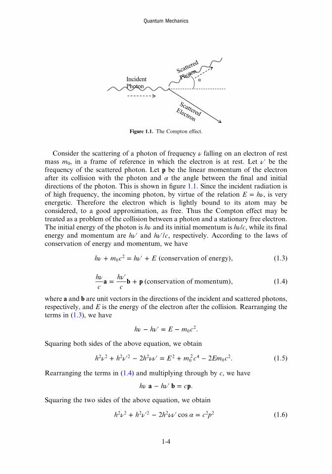
Consider the scattering of a photon of frequency ν falling on an electron of restmass m0, in a frame of reference in which the electron is at rest. Let ν′ be thefrequency of the scattered photon. Let p be the linear momentum of the electronafter its collision with the photon and α the angle between the final and initialdirections of the photon. This is shown in figure 1.1. Since the incident radiation isof high frequency, the incoming photon, by virtue of the relation E = hν, is veryenergetic. Therefore the electron which is lightly bound to its atom may beconsidered, to a good approximation, as free. Thus the Compton effect may betreated as a problem of the collision between a photon and a stationary free electron.The initial energy of the photon is hν and its initial momentum is hν/c, while its finalenergy and momentum are ν′h and ν′h c/ , respectively. According to the laws ofconservation of energy and momentum, we have

ν ν+ = ′ +h m c h E (conservation of energy), (1.3)02

ν ν= ′ +hc

hc

a b p (conservation of momentum), (1.4)

where a and b are unit vectors in the directions of the incident and scattered photons,respectively, and E is the energy of the electron after the collision. Rearranging theterms in (1.3), we have

ν ν− ′ = −h h E m c .02

Squaring both sides of the above equation, we obtain

ν ν νν+ ′ − ′ = + −h h h E m c Em c2 2 . (1.5)2 2 2 2 2 202 4

02

Rearranging the terms in (1.4) and multiplying through by c, we have

ν ν− ′ =h h ca b p.

Squaring the two sides of the above equation, we obtain

ν ν νν α+ ′ − ′ =h h h c p2 cos (1.6)2 2 2 2 2 2 2

Figure 1.1. The Compton effect.

Quantum Mechanics

1-4

where α is the angle between a and b. Substituting the expression for c2p2 from theequation = +E m c c p2

02 4 2 2 into (1.6), we obtain

ν ν νν α+ ′ − ′ = −h h h E m c2 cos . (1.7)2 2 2 2 2 202 4

Subtracting (1.5) from (1.7), we have

νν α ν ν′ − = − = − ′( )h m c E m c m c h h2 (1 cos ) 2 2 ( )20

20

20

2

where, in obtaining the expression on the extreme right, we have made use of (1.3).The above equation can be written as

α ν ννν ν ν

λ λ− = − ′′

=′

− = ′ −h

m c c c(1 cos )

1 1,

02

or

λ λ α′ − = −hm c

(1 cos ). (1.8)0

The quantity h/m0c is called the Compton wavelength and has the value 0.02426 ×10−8 cm. Equation (1.8) has been found to be consistent with experiments. For hiscontribution, Compton shared the Nobel Prize in physics in 1927.

Problem

1.1. Comment on the statement that in the photoelectric effect the photontransfers all of its energy while in the Compton effect only part of theenergy is transferred to the electron.

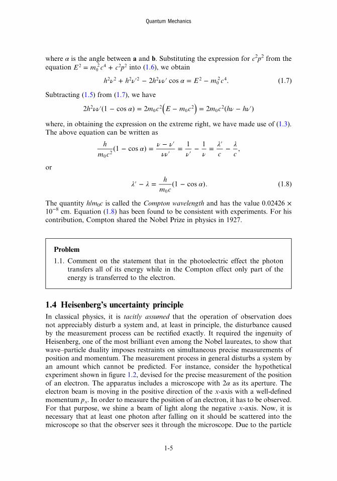
1.4 Heisenberg’s uncertainty principleIn classical physics, it is tacitly assumed that the operation of observation doesnot appreciably disturb a system and, at least in principle, the disturbance causedby the measurement process can be rectified exactly. It required the ingenuity ofHeisenberg, one of the most brilliant even among the Nobel laureates, to show thatwave–particle duality imposes restraints on simultaneous precise measurements ofposition and momentum. The measurement process in general disturbs a system byan amount which cannot be predicted. For instance, consider the hypotheticalexperiment shown in figure 1.2, devised for the precise measurement of the positionof an electron. The apparatus includes a microscope with 2α as its aperture. Theelectron beam is moving in the positive direction of the x-axis with a well-definedmomentum px. In order to measure the position of an electron, it has to be observed.For that purpose, we shine a beam of light along the negative x-axis. Now, it isnecessary that at least one photon after falling on it should be scattered into themicroscope so that the observer sees it through the microscope. Due to the particle

Quantum Mechanics

1-5

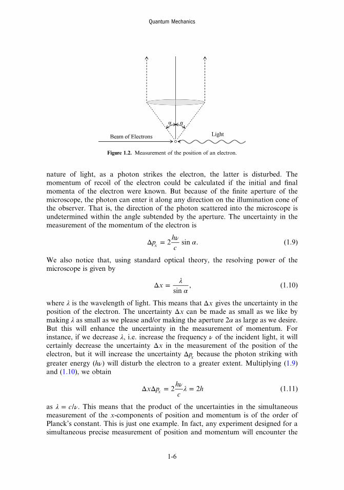
nature of light, as a photon strikes the electron, the latter is disturbed. Themomentum of recoil of the electron could be calculated if the initial and finalmomenta of the electron were known. But because of the finite aperture of themicroscope, the photon can enter it along any direction on the illumination cone ofthe observer. That is, the direction of the photon scattered into the microscope isundetermined within the angle subtended by the aperture. The uncertainty in themeasurement of the momentum of the electron is

ν αΔ =phc

2 sin . (1.9)x

We also notice that, using standard optical theory, the resolving power of themicroscope is given by

λα

Δ =xsin

, (1.10)

where λ is the wavelength of light. This means that Δx gives the uncertainty in theposition of the electron. The uncertainty Δx can be made as small as we like bymaking λ as small as we please and/or making the aperture 2α as large as we desire.But this will enhance the uncertainty in the measurement of momentum. Forinstance, if we decrease λ, i.e. increase the frequency ν of the incident light, it willcertainly decrease the uncertainty Δx in the measurement of the position of theelectron, but it will increase the uncertainty Δpx because the photon striking withgreater energy ( νh ) will disturb the electron to a greater extent. Multiplying (1.9)and (1.10), we obtain

ν λΔ Δ = =x phc

h2 2 (1.11)x

as λ ν= c/ . This means that the product of the uncertainties in the simultaneousmeasurement of the x-components of position and momentum is of the order ofPlanck’s constant. This is just one example. In fact, any experiment designed for asimultaneous precise measurement of position and momentum will encounter the

Figure 1.2. Measurement of the position of an electron.

Quantum Mechanics

1-6

same constraint. This is not an error in experimental measurement. It is inherent innature in the sense that it is due to the unavoidable interaction between the observerand the observed during the process of observation. The above analysis shows that asimultaneous precise measurement of position and momentum is impossible. This isknown as Heisenberg’s uncertainty principle or principle of indeterminacy. It can beshown that similar uncertainty relations exist between energy and time and angularmomentum and angle. In other words, a simultaneous precise measurement of twocanonically conjugate variables is impossible.

1.5 The correspondence principleAlthough classical mechanics breaks downwhen applied to determining the behaviourof tiny objects such as electrons, protons, etc, it has been providing correct answers tomechanical phenomena at the macroscopic level. Therefore, at this level, quantumtheory should be consistent with classical mechanics. This is known as Bohr’scorrespondence principle and is said to serve as a guide in discovering the correctquantum laws. In fact, under old conditions, a new theory should always yield the sameresults as the old theory which it is replacing, because the original theory has beenexplaining the experimental data in its own domain. In the case of quantummechanics,this correspondence may be specified by claiming that, for large quantum numbers,quantum theory must be consistent with classical physics. Moreover, if a quantumsystemhas a classical analogue, then for the limit h→ 0, it must yield the correspondingclassical results. Thus, in the uncertainty principle, as h → 0 in the classical limit, theproduct ΔxΔpx → 0 and therefore a simultaneous precise measurement of positionand momentum at macroscopic level becomes permissible. The importance of thecorrespondence principle lies not in stating that quantum theory should yield thesame results as classical mechanics at the macroscopic level, but in describingthe conditions under which it should happen.

1.6 The Schrödinger wave equationThere is no doubt that Planck’s quantum theory of black body radiation, Einstein’shypothesis of light quanta for the explanation of the photoelectric effect, Bohr’spostulates regarding the interpretation of the spectrum of the hydrogen atom and deBroglie’s hypothesis about the dual nature of matter were the milestones in theprogress of physics from 1900 to 1923. But physicists desired a differential equationwhich could govern the behaviour of mechanical phenomena and consequentlyexplain various experimental results. In 1926, Schrödinger set up such a differentialequation which is named after him and was supposed to replace Newton’s secondlaw of motion as the basic law of nature in mechanics. The mechanics based on thisdifferential equation was called wave mechanics and is now known as quantummechanics. Schrödinger’s differential equation undoubtedly outshone all the above-mentioned postulates and started commanding immense attention in the physicscommunity immediately after its advent. We will now set up this differentialequation. It must be clearly stated that the Schrödinger wave equation cannot belogically derived. The historical development may make its presence somewhat

Quantum Mechanics

1-7

plausible. But we will establish it by adopting an operational technique which isto-the-point and simple. We proceed as follows.

In terms of the kinetic energy T and the potential energy V of a particle, the non-relativistic classical expression for its total energy E is given by

= +E T V ,

where V is, in general, a function of space and time coordinates, V=V(r, t), but

= =T mm

vp1

2 2,2

2

where m is the mass, v is the velocity and p is the linear momentum of the particle.This yields

= +Em

Vp2

. (1.12)2

It is assumed that the transition from classical to quantum mechanics is made byinterpreting E, p and V as operators such that

→ ℏ ∂∂

Et

i , (1.13)

where ℏ =π

,h2

→ − ℏ∇p i , (1.14)

and

→V V . (1.15)

The operator ∇ is given by

∇ = ∂∂

+ ∂∂

+ ∂∂x y z

i j k,

where x, y, z are space coordinates and i, j, k are unit vectors along the x-, y- andz-axes. The time coordinate, wherever it occurs, is denoted by t. Note that while Eand p are interpreted as differential operators, the potential energy is assumed to beonly a multiplication operator, its form remaining unchanged when moving fromclassical to quantum mechanics. Equation (1.12) therefore yields

ℏ ∂∂

= − ℏ ∇ +t m

Vi2

,2

2

where

∇ ≡ ∂∂

+ ∂∂

+ ∂∂x y z

.22

2

2

2

2

2

Quantum Mechanics

1-8

If a function Ψ(x, y, z, t), which for convenience we may also write as Ψ(r, t) ormerely as Ψ, represents the particle under consideration, then operating thisequation on Ψ ≡ Ψtr( , ) and interchanging the two sides of the equation thusformed, we obtain

⎛⎝⎜

⎞⎠⎟− ℏ ∇ + Ψ = ℏ∂Ψ

∂mV

ta

2i , (1.16 )

22

or

Ψ = ℏ∂Ψ∂

Ht

bi , (1.16 )

where

⎛⎝⎜

⎞⎠⎟≡ − ℏ ∇ +H

mV c

2(1.16 )

22

is the Hamiltonian operator for the system. Equation (1.16a), equivalently (1.16b), is apartial differential equation in four independent variables and is known as the time-dependent Schrödinger wave equation. It is called a wave equation as it is similar to adifferential equation for waves. It is assumed to be the fundamental differentialequation governing the behaviour of mechanical phenomena. It replaces Newton’ssecond law of motion in mechanics. However, unlike Newton’s law of motion, it isnot garbed in words. This law of nature presents itself only as a differential equation.The function Ψ(r, t), a solution of the time-dependent Schrödinger wave equation fora system, is called a wave function and is necessarily a complex function because of thecomplex nature of the differential equation. It should not be considered to be a physicalwave. It is actually a mathematical function containing all the information that canbe obtained about the system it represents. The time-dependent Schrödinger waveequation is a linear partial differential equation of the first order in the time derivativeand of the second order in the spatial derivative. This implies that if its solution at aparticular time t0 is known, it can be calculated at any time t. But just as in the case ofNewton’s second law of motion, there is no logical derivation of the Schrödinger waveequation. It was a brilliant guess of Schrödinger in the perspective of the dual natureof matter. The ultimate test of a theory comes from its confrontation withexperimental data. And of course, for non-relativistic mechanical phenomena, thetheory based on Schrödinger’s wave equation has emerged successful.

Whenever we have to solve a physical problem in quantum mechanics, we resortto this equation, just as in classical mechanics we use the second law of motion. Towrite the Schrödinger wave equation for a particular system, we have to find theclassical expression for the potential energy V of the system and substitute it intoequation (1.16a). This gives us the desired differential equation which may be solvedto obtain a complex solution Ψ ≡ Ψtr( , ) . Since the differential equation containsonly a first-order time derivative, the wave function is uniquely prescribed, once itsvalue at a time t = t0 is known. But how is this function Ψ(r, t) interpreted so as to

Quantum Mechanics

1-9

relate it to physically measurable characteristics of the system? Certain prescriptionswere proposed but after facing insurmountable difficulties, on a suggestion by Born,a consensus was ultimately developed in the physics community. The complexfunction Ψ(r, t) representing the particle, being itself not directly observable, isinterpreted so that

Ψ Ψ* t t x y zr r( , ) ( , ) d d d

represents the probability of finding the particle in a small volume dxdydz (≡ dτ) aboutthe point r and at time t. It must be emphasised that this interpretation is only ahypothesis. Its validity is established by the success of its predictions. No doubt, thetime evolution of the wave function Ψ(r, t) is inextricably connected to probabilisticconcepts. It has been rightly stated, in flowery language, that Ψ Ψ* is the windowthrough which we can view the world of the atom. Schrödinger himself was shockedwhen he was told about the statistical interpretation of quantum mechanics. He oncetold Bohr ‘If we are going to stick to this damned quantum jumping, then I regretthat I ever had anything to do with quantum theory’. Bohr quipped ‘But the restof us are thankful that you did’. To this interpretation, which demolishes thedeterminism of classical mechanics, Schrödinger and Einstein could not reconcilethemselves, even to the last days of their lives. The total probability of finding theparticle in a volume in which it is confined is

∫ ∫τ τΨ Ψ ≡ Ψ* *( )t t tr r r( , ) ( , ) d ( , ) d2

and must be 100%, i.e. 1, because the particle must be somewhere in that volume.Hence we may write

∫ τΨ Ψ =* t tr r( , ) ( , ) d 1. (1.17)

The wave function Ψ(r, t) is then said to be normalised to unity or simply normalised.The above equation is said to express the normalisation condition. This equationexists only if the integral

∫ τΨ Ψ* t tr r( , ) ( , ) d

converges, i.e. it is finite; for instance, if the wave function goes to zero sufficientlyrapidly as r tends to infinity. The functionΨ(r, t) is then said to be square integrable orto have an integrable square. Symbolically, in this case, Ψ(r, t)→ 0 as ∣r∣→∞. This isthe boundary condition which is always satisfied when the state is bound. Forinstance, an electron bound to the hydrogen nucleus, constitutes the hydrogen atom—

a bound state. For such a state, the particle can never go to infinity. The integral

∫ ∫τ τΨ Ψ ≡ Ψ* t t tr r r( , ) ( , ) d ( , ) d2

exists and the function Ψ(r, t) can be normalised. In certain cases, for instance for afree particle, the above integral may diverge. Then a somewhat different formulation

Quantum Mechanics

1-10

of the normalisation condition is to be given which will be considered at a later stage.Ψ*(r, t)Ψ(r, t) is the probability density, i.e. the probability per unit volume. Noticethat the statement in the above form about the probability is valid only if Ψ(r, t) isnormalised. It may be emphasised that the above prescription incorporates thestatistical interpretation in the basic differential equation, the Schrödinger waveequation. Since this is a homogeneous, linear differential equation, if Ψ(r, t) is asolution of this differential equation, then CΨ(r, t) is also a solution of the samewhere C is a constant. In most cases, the value of C can be determined by using thenormalisation condition.

In one-dimensional space, Ψ*(x, t)Ψ(x, t) dx is interpreted as the probability offinding the particle in the length dx between x and x + dx at time t.

It is important to state at this stage that we have only interpreted Ψ so as to relateit to the probability distribution. Actually, we have to compute various physicalquantities, representing dynamical variables in classical mechanics, such as position,linear momentum, energy and components of angular momentum, so that we maycompare our theoretical results with experimental data. Another postulate is to beproposed for this purpose. Since new concepts are involved, we will consider it laterin this chapter when these concepts have been introduced.

1.7 Constraints on solutionsEvery solution of the Schrödinger wave equation is not physically acceptable. Theabove interpretation of Ψ*(r, t)Ψ(r, t) dτ as the probability of finding the particle inthe small volume dτ about r and at time t imposes certain constraints on the solutionΨ(r, t) of this second-order partial differential equation. In fact, in order for thesolution to be physically acceptable, it must be well-behaved, i.e. the wave functionshould be finite, single valued and continuous. Moreover, its first derivatives withrespect to space co-ordinates must be continuous. This is analysed below.

1. The function Ψ(r, t) must be finite for all values of x, y, z. In fact, Ψ(r, t)should be such that it vanishes sufficiently rapidly as infinity is approached soas to give us no trouble; the function remains square integrable. This is sobecause otherwise the probability of finding the particle in the small regionabout a point where the function diverges will become infinite which isphysically unacceptable.

2. The function Ψ(r, t) must be single-valued, i.e. for each set of the values ofthe variables it should have only one value. This is essential becauseotherwise the probability of finding the particle at a particular point andat a certain time will not be unique; it will have more than one value, eachvalue depending upon the choice of the multivalued function Ψ(r, t) such as

−tan 1x. Strictly speaking, according to this argument, it is Ψ*(r, t)Ψ(r, t)which should be single-valued. However, successful results for the character-istics of some physical quantities, such as the z-component of orbital angularmomentum, require that the wave function be single-valued.

3. The function Ψ(r, t) and its first derivatives with respect to space co-ordinatesshould be continuous in all parts of the region.

Quantum Mechanics

1-11

Before considering the last characteristic in detail, let us recall a mathematicaltheorem: a function continuous at a point is not necessarily differentiable there but afunction differentiable at a point is necessarily continuous there. Thus if a function f isdifferentiable at a point, i.e. if df/dx exists at a point, then f must be continuousthere. Similarly, if d2f/dx2 exists, then df/dx must be continuous there. To makethings simple, consider the time-dependent Schrödinger wave equation in one-dimension,

⎛⎝⎜

⎞⎠⎟− ℏ ∂

∂+ Ψ = ℏ∂Ψ

∂m xV

t2i . (1.18)

2 2

2

Rearranging the terms, we have

Ψ = ℏ ∂ Ψ∂

+ ℏ∂Ψ∂

Vm x t2

i .2 2

2

We will consider the case when the potential energy of a physical system is finite,whether continuous or with a number of finite discontinuities, because infiniteenergies do not occur in nature. Then the left-hand side of the above equation isfinite. Consequently, both the terms on the right-hand side should be finite. Thus, as∂2Ψ/∂x2 is finite, i.e. the differential coefficient of ∂Ψ/∂x exists, the function ∂Ψ/∂xmust be continuous. Moreover, as ∂Ψ/∂x exists, i.e. the differential coefficient of Ψexists, the function Ψ must be continuous. Hence, the condition that the wavefunction and its first space derivative should be continuous is a requirement imposedby the finiteness of Ψ and consistency of the Schrödinger wave equation. The analysiscan easily be extended to three dimensions.

It can be mentioned that if Ψ is assumed to be continuous, then we need notassume that it is finite because every continuous function is finite.

Owing to the requirement that the function Ψ(r, t) must be well-behaved and itsfirst derivative with respect to the space coordinate should be continuous, all themathematical solutions of the Schrödinger wave equation are not physicallyacceptable. This in turn means that for a physical system, only those energies willbe allowed which correspond to physically acceptable wave functions. We will findthat by the requirement of admissible wave functions, energy and some otherphysical quantities are quantised.

The time-dependent Schrödinger wave equation is of first order in the time-derivative. Therefore, if the wave function Ψ(r, t0) at any initial time t0 is known, thewave function Ψ(r, t) at any time t can be calculated.

Problem

1.2. Comment on the remark that the assumptions that the wave function befinite and single-valued at all points in configuration space may be morerigorous than necessary.

Quantum Mechanics

1-12

Remark

If Ψ is finite and V is continuous or has finite discontinuities, then theconsistency of the Schrödinger wave equation requires that Ψ and its firstspace derivative should be continuous. It may be emphasised that it is not aconsequence of the probabilistic interpretation of Ψ. This is a characteristic ofcertain types of second-order differential equations.

1.8 Eigenfunctions and eigenvaluesBefore we proceed further, we will define a few terms and illustrate them with thehelp of examples. We first define the eigenfunctions and eigenvalues of any operator.Consider an operator A operating on a function ϕ such that

ϕ λϕ=A , (1.19)

that is, it reproduces the function ϕ multiplying it with a constant λ. Then thefunction ϕ is called an eigenfunction (or characteristic function) of the operator Awith eigenvalue (or characteristic value) λ or corresponding to the eigenvalue λ. Theequation itself is called an eigenvalue equation (or characteristic equation). Thus, inthe eigenvalue equation

= −x

x xd

d(sin 3 ) 9(sin 3 ),

2

2

−9 is the eigenvalue of the operator d2/dx2 corresponding to the eigenfunctionsin 3x.

An operator has several eigenfunctions with the corresponding eigenvalues. Theseeigenvalues may be discrete or continuous. If the eigenvalue spectrum is discrete, thevalues are written as, say, λ1, λ2, λ3,…. If the eigenvalue spectrum is continuous, thevalues are denoted by λ′, λ″, λ‴,…. The eigenvalue spectrum may be partiallydiscrete and partially continuous. For simplicity, in general analysis, as far aspossible, we will be considering only discrete eigenvalues.

A set of functions ϕ1, ϕ2,…, ϕn is said to be linearly independent if its linearcombination a1ϕ1 + a2ϕ2 +⋯+ anϕn cannot be made equal to zero for all values ofthe variables except by taking all a equal to zero. For instance, sin x and cos x are twolinearly independent functions as their linear combination, a1 sin x + a2 cos x, cannotbe made equal to zero for all values of the variable x except by taking a1 = a2 = 0.

Suppose that ϕ1, ϕ2,…, ϕn are n linearly independent eigenfunctions of anoperator A corresponding to the same eigenvalue λ. Then we may write

ϕ λϕϕ λϕ

ϕ λϕ

==⋯=

A

A

A

,

,

.

(1.20)

n n

1 1

2 2

Quantum Mechanics

1-13

The number λ is called an n-fold degenerate eigenvalue of the operator A,corresponding to linearly independent eigenfunctions ϕ1, ϕ2,…, ϕn. These eigenfunc-tions are called n-fold degenerate, corresponding to the same eigenvalue λ. Thenumber n is called the degree of degeneracy of the eigenfunctions.

Problem

1.3. Show that −4 is a two-fold degenerate eigenvalue of the operator d2/dx2

corresponding to linearly independent eigenfunctions sin 2x and cos 2x.

1.9 The principle of superpositionWe have seen that the time-dependent Schrödinger wave equation can be written as

Ψ = ℏ∂Ψ∂

′Ht

bi . (1.16 )

For convenience, changing the two sides of the above equation, we obtain

ℏ∂Ψ∂

= Ψt

Hi . (1.21)

Let Ψ1 and Ψ2 be two solutions (maybe belonging to different values of energy) ofthis differential equation so that

ℏ∂Ψ∂

= Ψt

Hi (1.22)11

and

ℏ∂Ψ∂

= Ψt

Hi . (1.23)22

It can easily be verified that a linear combination of these solutions, i.e. a1Ψ1 + a2Ψ2,is also a solution of the Schrödinger wave equation. This is shown below:

ℏ ∂∂

Ψ + Ψ = ℏ∂Ψ∂

+ ℏ∂Ψ∂

= Ψ + Ψ

= Ψ + Ψ )

( )t

a a at

at

a H a H

H a a

i i i

( . (1.24)

1 1 2 2 11

22

1 1 2 2

1 1 2 2

In fact, we could directly state that as Schrödinger’s second order time-dependentpartial differential equation is linear (because the function Ψ and its derivativesoccur only to the first degree and not as higher powers or products), every linearcombination of its solutions is also a solution of this differential equation. This isknown as the principle of superposition and plays a very important role in quantummechanics. It can be mentioned that this is a characteristic of every homogeneouslinear differential equation.

Quantum Mechanics

1-14

This is the right moment to point out that in classical mechanics, knowledgeabout the position and momentum of a particle at any time describes what is calledthe state of the particle. If we know the position and momentum of a particle atany time, then we can compute its position and momentum at any other time byusing the second law of motion. This implies that if the initial state of the system isgiven, the values of all other variables can be determined exactly for all times. Inquantum mechanics, according to Heisenberg’s uncertainty principle, position andmomentum cannot be measured precisely at the same time. Therefore, the state ofthe particle in the classical sense cannot be described. Hence, in quantum mechanics,there is no concept of the trajectory of a particle as it is determined by asimultaneous precise knowledge of position and momentum at every moment;such a trajectory does not exist when quantum effects are important as it is thenimpossible to keep track of the particle. However, all the accessible informationabout the particle is contained in the wave function Ψ. Naturally, the question arises:how do we define the state of a particle in quantum mechanics? In fact, we assume asa fundamental principle of quantum mechanics that every physically acceptablesolution of the Schrödinger wave equation represents a state of the system. The time-dependent Schrödinger wave equation is a linear partial differential equation of firstdegree in the time variable. Therefore, if Ψ is known at a particular time t0, it can bedetermined at any time t. Suppose that Ψ1 and Ψ2 represent two states of a systemwhich correspond to definite energy values, say E1 and E2. These states are thencalled eigenstates of the system. Since a linear combination of these solutions, a1Ψ1 +a2Ψ2, where a1 and a2 are (complex) numbers, is itself a solution of this differentialequation, it also represents a state of the system. However, this state does notcorrespond to a definite energy. Such a state is called a quantum state of the system.It has no analogue in classical mechanics where each state, like an eigenstate inquantum mechanics, corresponds to a definite energy. Now suppose that thefunctions Ψ1(t0) and Ψ2(t0) are two solutions of the Schrödinger wave equation attime t0. Let

Ψ = Ψ + Ψt a t a t( ) ( ) ( )0 1 1 0 2 2 0

be a linear superposition of Ψ1(t0) and Ψ2(t0) at time t0. Suppose that the functionsΨ1(t0) and Ψ2(t0) develop with time into functions Ψ1(t) and Ψ2(t). Then, by virtue ofthe fact that the Schrödinger wave equation is linear in Ψ, we must have

Ψ = Ψ + Ψt a t a t( ) ( ) ( ),1 1 2 2

i.e. at any time t, Ψ(t) is the same linear combination of the functions Ψ1(t) and Ψ2(t).The fact that the first of these equations entails the second equation is a consequenceof the linearity of the time development of a state.

An overview of various disciplines of physics shows that the principle ofsuperposition is one of the most significant attributes of the wave concept. It iscommon to all types of waves. We may transcend a step higher than this and take itas a characteristic of every homogeneous linear differential equation: a linear

Quantum Mechanics

1-15

superposition of the solutions of a homogeneous linear differential equation is also asolution of this differential equation. Quantum mechanics which emphasises thisformal aspect was developed by Dirac, a British Nobel laureate. It describes thepossible states of a system by abstract quantities called state vectors which obey theprinciple of superposition. Indeed, the essence of this principle as reflected bystate vectors is much more attractive than that predicted by wave functions.

A quantity which can be measured is called an observable. In classical physics,observables are represented by ordinary variables. In quantum mechanics, however,observables are, by assumption, represented by operators. It is customary in theliterature to use the same letter for the observable, variable and operator. We willalso adopt this convention.

1.10 ComplementarityThe statistical interpretation of the wave function and Heisenberg’s principle ofuncertainty are the concepts with which some eminent physicists of the good olddays were finding it difficult to come to terms. Bohr therefore devoted his fullattention to detailed analyses of various new concepts which were leading to newtrends in scientific attitudes and its philosophical consequences. His analysis thatthe wave and particle aspects of matter are opposing but complementary modes ofits realisation has been named the principle of complementarity. This is the essenceof his views on the conceptual basis of quantum mechanics but it does not help inmaking calculations in this field. In fact, classical physics, based upon the knowl-edge gained from every day experience, i.e. from the behaviour of macroscopicobjects, tells us that an object in nature can behave either as a particle or as a wave.It cannot exhibit both characteristics. According to the principle of complemen-tarity, analysis at a microscopic level reveals that an object can behave both asa particle and a wave but the two modes cannot be realised at the same time.A measurement which emphasises one of the wave–particle attributes does so at theexpense of the other. An experiment designed to exhibit the particle properties doesnot give any information on the wave aspect and vice versa. For instance, theobservation of cloud chamber tracks does not involve wave aspect at all whileinterference and diffraction experiments do not contain any information aboutthe particles’ demeanour. It is interesting to note that all possibly availableknowledge about the characteristics of a microscopic entity, say an electron, iscontained in the wave function. We will express it like this. A microscopic entityunder one situation shows those properties which at macroscopic level areattributed to particles and we say that it is behaving as a particle. In some othersituation, the same entity exhibits characteristics which at macroscopic level areassigned to waves. Then we say that the entity is behaving as a wave. Actually, thebehaviour is determined by the same wave function and it is different, as it must be,under different circumstances. We are surprised simply because it is not what wewere expecting from our experience in everyday life. But nature does behave thatway and sometimes it produces results even against those expectations which arebased on very careful considerations and analysis!

Quantum Mechanics

1-16

1.11 Schrödinger’s amplitude equationWe will now show that the computations in solving the Schrödinger wave equationare simplified if the potential energy V of the system does not depend upon timeexplicitly: V≡V(x, y, z)≡V(r). Let us assume that in this case the wave functionΨ(r, t) representing the particle can be expressed as a product of two functions, onedepending only on space coordinates and the other depending on time alone. If wedenote these functions, respectively, by ψ(x, y, z) (also written as ψ(r)) and ϕ(t), thenwe may write

ψ ϕΨ =x y z t x y z t( , , , ) ( , , ) ( ). (1.25)

Differentiating twice with respect to x, we obtain

ψ ϕ∂ Ψ∂

= ∂∂x x

. (1.26)2

2

2

2

where Ψ≡ Ψ(x, y, z, t)≡ Ψ(r, t), ψ≡ ψ(x, y, z) ≡ ψ(r) and ϕ ≡ ϕ(t). We can obtain twosimilar expressions for the second-order derivatives with respect to space coordinatesy and z. Next, differentiating (1.25) with respect to t, we obtain

ψ ϕ∂Ψ∂

=t t

dd

. (1.27)

Notice that for the function ϕ, we have used the ordinary derivative instead of thepartial derivative as this function depends upon one variable t only. Substituting theexpressions from (1.26), etc, and equation (1.27) in equation (1.16a), we obtain

⎡⎣⎢

⎤⎦⎥

ψ ϕ ψ ϕ ψ ϕ ψϕ ψ ϕ− ℏ ∂∂

+ ∂∂

+ ∂∂

+ = ℏm x y z

V x y zt2

( , , ) idd

,2 2

2

2

2

2

2

or

ψ ϕ ψϕ ψ ϕ− ℏ ∇ + + ℏ( )m

Vt2

idd

.2

2

Dividing throughout by ψϕ, we obtain

ψψ

ϕϕ− ℏ ∇ + = ℏ( )

mV

t21

i1 d

d. (1.28)

22

The right-hand side of this equation is a function of time only while, as V dependsexplicitly only on space coordinates, the left-hand side depends upon spacecoordinates alone. Therefore, a variation in space coordinates will not affect theright-hand side while a variation in time will not affect the left-hand side. This ispossible only if each side is equal to the same constant. We denote this constant by E.Then we may write

ϕϕℏ =t

Ei1 d

d(1.29)

Quantum Mechanics

1-17

and

ψψ− ℏ ∇ + =( )

mV E

21

,2

2

or

⎛⎝⎜

⎞⎠⎟ψ ψ− ℏ ∇ + =

mV E

2. (1.30)

22

This is called the Schrödinger amplitude equation. The operator in brackets in theabove equation is the Hamiltonian operator H of the particle. The amplitudeequation therefore can be written as

ψ ψ=H E . (1.31)

It is called the Hamiltonian form of the Schrödinger amplitude equation. This is aneigenvalue equation. The constant E is the eigenvalue of the Hamiltonian operatorH corresponding to the eigenfunction ψ. The Schrödinger amplitude equation thustakes the form of an eigenvalue equation for the Hamiltonian H and this simplifiesthe analysis of the problem.

Let us first solve the differential equation (1.29) involving only time as anindependent variable. Transposing iℏ to the right-hand side of this differentialequation and integrating with respect to time t, we obtain

ϕ = −ℏ

+tEt

Kln ( )i

.

Choosing the initial condition that makes K = 0, we obtain

ϕ = −ℏ

tEt

ln ( )i

,

or

⎛⎝⎜

⎞⎠⎟ϕ = −

ℏt

Et( ) exp

i. (1.32)

The expression in brackets on the right-hand side shows that E has the dimensions ofenergy. We will assume here but will prove later on that E is the total energy of thesystem.

Let us next consider the differential equation (1.30) that can be written as

ψ ψ∇ +ℏ

− =mE V

2( ) 0. (1.33)2

2

This is the time-independent Schrödinger wave equation or the amplitude equationor the steady-state Schrödinger equation. This differential equation for a systemcan be solved only if the expression for the potential energy of the system is known.

Quantum Mechanics

1-18

The solution of this differential equation is denoted by ψ(r). Equation (1.25) can nowbe written as

⎛⎝⎜

⎞⎠⎟ψΨ = −

ℏt

Etr r( , ) ( ) exp

i,

where for convenience we have written r for x, y, z. If we are interested in finding thecharacteristics of a physical system whose potential energy does not depend explicitlyon time, then instead of using the time-dependent Schrödinger equation, which isrelatively much more difficult to solve, we can use the time-independent Schrödingerequation which is easier to solve. We obtain the solution ψ(r) of this differentialequation and multiply it by ϕ(t) (≡ exp(−iEt/ℏ)) so as to obtain Ψ(r, t) whichrepresents the system. Then a wave function of the system corresponding to adefinite energy can be written as

⎛⎝⎜

⎞⎠⎟ψ ϕ ψΨ = = −

ℏt t

Etr r r( , ) ( ) ( ) ( ) exp

i. (1.34)

Thus

ψΨ Ψ = Ψ* *t tr r r r( , ) ( , ) ( ) ( ). (1.35)

The above analysis shows that the probability density for a particle whose potentialenergy does not depend upon time explicitly is constant in time. For this reason, awave function of the form (1.34) is said to represent a stationary state or an energyeigenstate of the particle. The energy in a stationary state is said to be sharp or well-defined. It can be said that although the wave function Ψ(r, t) representing theparticle is time-dependent, the probability density is independent of time. Therefore,the system would remain in that state indefinitely. Every measurement will alwaysgive the same value of energy. This interpretation is consistent with the uncertaintyrelation

Δ Δ ∼ ℏE t ,

as this means that if the system is in an eigenstate with definite energy so that ΔE = 0,then unlimited time should be available to make that measurement. If the energyspectrum is discrete, the lowest energy state is called the ground state of the system.The higher energy states are called excited states of the system.

For a stationary state, the normalisation condition,

∫ τΨ Ψ =* t tr r( , ) ( , ) d 1,

is simplified to

∫ ∫ψ τ ψ ψ τΨ = =* ℏ − ℏ *r r r r( )e ( )e d ( ) ( ) d 1. (1.36)Et Eti / i /

Quantum Mechanics

1-19

In one dimension, the time-independent Schrödinger wave equation reduces to thefollowing form:

ψ ψ+ℏ

− =x

mE V

d

d

2( ) 0, (1.37)

2

2 2

where ψ ≡ ψ(x). It is important to note that the amplitude function ψ(x), a solutionof the Schrödinger amplitude equation and related to the wave function Ψ(x, t) by

⎛⎝⎜

⎞⎠⎟ψ ϕ ψΨ = = −

ℏx t x t x

Et( , ) ( ) ( ) ( ) exp

i, (1.33')

should also be well-behaved. This is because if ψ(x) is not finite, then Ψ(x, t) will alsobe not finite and if ψ(x) is not single-valued, then Ψ(x, t) will also not be single-valued. This is due to the fact that the time function ϕ(t) is always finite and does notdepend upon space coordinates. As far as the continuity of the function ψ(x) and itsfirst derivative dψ/dx is concerned, we note from (1.37) that as ψ(x) is always finiteand infinite energies cannot be achieved in nature, the first term on the left-handside of this equation, i.e. the second derivative of ψ(x), should also be finite.Therefore, dψ/dx must be continuous. Moreover, as dψ/dx exists, the function ψ(x)should be continuous. Thus, the very consistency of the Schrödinger amplitudeequation requires that both ψ(x) and dψ(x)/dx should be continuous.

Infinite energies do not occur in nature. But let us see what will happen if at somepoint the potential jumps from a finite to an infinite value. Equation (1.37) showsthat in this case d2ψ/dx2 will be infinite. Therefore, dψ/dx may or may not becontinuous. That is, the condition of continuity of the space derivative of the wavefunction at the discontinuity of the potential cannot be imposed. However, as dψ/dxexists because otherwise the differential equation will not hold, the function ψ(x) willbe continuous. In the solution of the eigenvalue equation Hψ = Eψ for a physicalsystem, we will find that the energy eigenvalues very much depend upon theconditions imposed on the solutions to the eigenvalue equation. We take thisopportunity to point out that it is not necessary that the integration should always beover the entire space extending from −∞ to +∞.

1.12 The orthonormal set of functionsConsider a set of functions ϕ1, ϕ2, ϕ3, … which are individually normalised, i.e.

∫ ϕ ϕ τ = = …* id 1, 1, 2, 3, (1.38)i i

and mutually orthogonal, i.e.

∫ ϕ ϕ τ = ≠ = …* j i i jd 0, , , 1, 2, 3, (1.39)i i

Quantum Mechanics

1-20

They are said to form an orthonormal set of functions. These two conditions for anorthonormal set can be expressed as

∫ ϕ ϕ τ δ=* d , (1.40)i j ij

where the Kronecker delta is defined as

δ = =j I1, for ,ij

δ = ≠j i0, for .ij

1.13 The equation of continuityWe know that any solution Ψ(r, t) of the time-dependent Schrödinger wave equationis such that

ρ = Ψ Ψ* t tr r( , ) ( , ) (1.41)

is interpreted as the probability density, i.e. the probability of finding the particle inunit volume about the point r and at time t. Differentiating with respect to time,we obtain

ρ∂∂

= ∂∂

Ψ Ψ = ∂Ψ∂

Ψ + Ψ ∂Ψ∂

**

*

t t t t( ) . (1.42)

But by virtue of equation (1.16a), i.e.

⎛⎝⎜

⎞⎠⎟ψ− ℏ∂Ψ

∂= − ℏ ∇ +

t mVi

2

22

and its complex conjugate

⎛⎝⎜

⎞⎠⎟ψ− ℏ∂Ψ

∂= − ℏ ∇ +

**

t mVi

2,

22

(1.42) yields

⎛⎝⎜

⎞⎠⎟

⎛⎝⎜

⎞⎠⎟

ρ

ψ ψ ψ ψ

ψ ψ

− ℏ ∂∂

= − ℏ∂Ψ∂

Ψ + − ℏ Ψ ∂Ψ∂

= − ℏ ∇ + Ψ − Ψ − ℏ ∇ +

= − ℏ Ψ∇ − Ψ ∇

**

* * *

* *( )

t t t

mV

mV

m

i i ( i )

2 2

2,

22

22

22 2

Quantum Mechanics

1-21

or

ρ ψ ψ

ψ ψ

∂∂

= − ℏ Ψ∇ − Ψ ∇

= − ℏ ∇ Ψ∇ − Ψ ∇

* *

* *

( )

( )t m

m

i2i2

. (1.43)

2 2

If we write

− ℏ Ψ ∇Ψ − Ψ∇Ψ =* *( )m

ji2

, (1.44)

then (1.43) can be expressed as

ρ∂∂

+ ∇ =t

j 0,

or

ρ∂∂

+ =t

jdiv 0. (1.45)

This is the well-known equation of continuity. This equation also arises in electro-magnetic theory and expresses the conservation of charge. If ρ represents the chargedensity, i.e. the charge per unit volume, and j = ρv is the current density, i.e. the chargepassing unit area normal to its direction of motion in one second, then the equationof continuity expresses the law of conservation of charge. The charge which isdecreasing with time in a bounded volume is accounted for by the charge which iscrossing the surface of the bounded volume. In quantum mechanics, ρ is interpretedas probability density. Therefore, if j is interpreted as the probability current density,then the equation of continuity guarantees the conservation of probability. Thus, ifthe probability of finding a particle in a certain bounded region decreases with time, itshould correspond to the increase in probability of finding it outside that region. Theprobability current density is also called the probability flux. It is given by

= − ℏ Ψ ∇Ψ − Ψ∇Ψ = ℏ Ψ ∇Ψ* * *( ) ( )m m

ji2

Im . (1.46)

Problem

1.4. Prove that

= ℏ Ψ ∇Ψ*( )m

j Im . (1.47)

Quantum Mechanics

1-22

We will now prove that the total probability of finding the particle in space isindependent of time. For one-dimensional space, we have

ρ = Ψ Ψ*x t x t x t( , ) ( , ) ( , ). (1.41')

Integrating with respect to x and then differentiating with respect to t, we obtain

∫ ∫ρ = Ψ Ψ−∞

∞

−∞

∞*

tx t x

tx t x t x

dd

( , ) ddd

( , ) ( , ) d . (1.48)

But, in one-dimensional space, we have

⎛⎝⎜

⎞⎠⎟− ℏ ∂

∂+ Ψ = ∂Ψ

∂′

m xV x x t h

x tt

a2

( ) ( , ) i( , )

. (1.16 )2 2

2

Taking the complex conjugate of both sides of equation (1.16a′), we obtain

⎛⎝⎜

⎞⎠⎟− ℏ ∂

∂+ Ψ = − ∂Ψ

∂*

*

m xV x x t h

x tt2

( ) ( , ) i( , )

. (1.49)2 2

2

Substituting these expressions for ∂Ψ*(x, t)/∂t and ∂Ψ(x, t)/∂t in (1.48) andsimplifying, we obtain

⎛⎝⎜

⎞⎠⎟

⎡⎣⎢⎢

⎛⎝⎜

⎞⎠⎟

⎤⎦⎥⎥

∫ ∫ρ = − ℏ ∂∂

Ψ ∂Ψ∂

+ Ψ ∂Ψ∂

= − ℏ Ψ ∂Ψ∂

+ Ψ ∂Ψ∂

=

−∞

∞

−∞

∞

−∞

∞ **

**

tx t x

m xx t

x tt

x tx tt

x

mx t

x tt

x tx tt

dd

( , ) di2

( , )( , )

( , )( , )

d

i2

( , )( , )

( , )( , )

0. (1.50)

The last result has been obtained because the wave function Ψ(x, t)→ 0 as x→∞ sothat the integral

∫ Ψ Ψ−∞

∞* x t x t x( , ) ( , ) d

may converge.Equation (1.50) shows that the total probability is conserved. This also ensures

that the normalisation is preserved: if the wave function is normalised, it will remainnormalised.

1.14 Complete sets of functionsA set of functions ψ1(x), ψ2(x), … in a variable x is said to form a complete set if anarbitrary square integrable function ϕ(x) can be expanded in terms of them:

∑ϕ ψ=x a x( ) ( ), (1.51)i

i i

Quantum Mechanics

1-23

where ai are called expansion coefficients. The values of ai can be obtained asfollows. Multiplying equation (1.51) by ψ *

j (x) and integrating with respect to x, weobtain

∫ ∫∑ψ ϕ ψ ψ=* *x x x a x x x( ) ( ) d ( ) ( ) d . (1.52)ij i j i

If the functions ψ1(x), ψ2(x), … form an orthonormal set, then

∫ ψ ψ δ=* x x x( ) ( ) d .j i ji

Therefore, (1.52) reduces to

∫ ∑ψ ϕ δ=* x x x a x( ) ( ) d ( ).ij i ij

Summing over i, and finally changing j to i throughout the equation, we obtain

∫ ψ ϕ= *a x x x( ) ( ) d . (1.53)i i

This equation determines all the expansion coefficients.

1.15 The quantum theory of measurementWe will now analyse the process of measurement in quantum mechanics in detail.We will concentrate on how to compute the physical quantities which are to becompared with the experiment. In fact, whenever we want to make an accuratemeasurement of any quantity, we measure that quantity a large number of timesand take the arithmetic mean of the measured values. This is called the average ormean value of the variable. The average value of a variable x is denoted by x̄:

¯ =+ + ⋯ +

xx x x

n. (1.54)n1 2

In order to have an idea about the precision of the various values we must know thescattering or dispersion of these individual values about their average. The individualdeviations from the mean are

− ¯ − ¯ … − ¯x x x x x x, , , .n1 2

But the average of these deviations is equal to

− ¯ + − ¯ + ⋯ + − ¯ =+ + ⋯ +

− ¯ = ¯ − ¯ =x x x x x x

n

x x x

nnxn

x x( ) ( ) ( )

0n n1 2 1 2

This shows that whatever the deviations of x from its mean value, the average ofthese deviations is always zero. The average of these deviations is therefore notuseful as a standard for measuring dispersion. Its value, being always zero, cannottell us whether the individual values are close to or far away from the average.

Quantum Mechanics

1-24

Perhaps a better idea about the dispersion of the values of a variable about theirmean can be obtained if we consider the average of the square of deviations of thevariable x from its mean value x̄. This is called the variance of x and is denoted by σ.Thus, we may write:

σ=

=− ¯ + − ¯ + ⋯ + − ¯

=+ + ⋯ +

+ ¯ − ¯+ + ⋯ +

= ¯ + ¯ − ¯ ¯= ¯ + ¯ − ¯= ¯ − ¯

x

x x x x x x

n

x x x

nnxn

xx x x

n

x x xx

x x x

x x

(Variance of )

( ) ( ) ( )

2

2

2

. (1.55)

n

n n

12

22 2

12

22 2 2

1 2

2 2

2 2 2

2 2

The positive square root of the variance of a variable x is called the standarddeviation of x or the root mean square deviation or the uncertainty in the value of xand is denoted by Δx. Thus

Δ = + ¯ − ¯x x x . (1.56)2 2

1.16 Observables and expectation valuesAs already mentioned, in quantum mechanics, each physical quantity (or attributeor property) which can be measured experimentally is called an observable and isrepresented by an operator. For instance, the energy of a system is an observableand is represented by the Hamiltonian operator H. Linear momentum is anotherobservable and is represented by the linear momentum operator −ih∇. The state of aphysical system is a collection of observables and is specified by the wave functionrepresenting the system. It is therefore common in the literature to use the termeigenstate to indicate a state represented by an eigenfunction. The average value,usually called the expectation value, of a sequence of measurements of an observablerepresented by an operator A(r, −iℏ∇, t) on a system in a normalised state describedby Ψ is, by definition, given by

∫ τ≡ ¯ = Ψ − Ψ*A A t A tr r( , ) ( , ) d . (1.57)

Frequently, the expectation value of a physical quantity represented by an operatorA is denoted by ⟨A⟩, i.e. the angle brackets are usually used for expectation values.Moreover, it is customary to use the same symbol for a dynamical variable as well asthe operator which represents it. It may again be remarked that in quantummechanics, a physical system is represented by a wave function such that our entiretheoretical knowledge about it is contained in the wave function. Since the

Quantum Mechanics

1-25

interpretation of the wave function is statistical in nature, laws of physics can onlymake probabilistic predictions. They cannot predict the precise behaviour of asystem. In other words, if a physical quantity is measured a large number of times byrepeating an experiment under identical conditions or by performing a large numberof identical experiments, its average value can be predicted by the above relation. Itshould be noted that, in general, the result of a single measurement will not be givenby ⟨A⟩. It is only the average value of a large number of measurements, made inthe manner suggested above, which is to be compared with the theoretical valuepredicted by equation (1.57). It may be emphasised that laws of physics arestatistical in nature even when we are dealing with a single particle.

If the wave function is not normalised, then the expectation value ⟨A⟩ is definedby the equation

∫∫

τ

τ=

Ψ Ψ

Ψ Ψ

*

*A

t A t

t t

r r

r r

( , ) ( , ) d

( , ) ( , ) d

which reduces to equation (1.57) for a normalised wave function.Let us now calculate the uncertainty in the measurement of a physical quantity

represented by an operator A when the system is represented by a normalisedeigenfunction Ψn of the operator A corresponding to the eigenvalue λn. Then

λΨ = ΨA (1.58)n n n

and the expectation values of A and A2 are given by

∫ ∫∫

τ λ τ

λ τ λ

= Ψ Ψ = Ψ Ψ

= Ψ Ψ =

* *

*

A t A t t t

t t

r r r r

r r

( , ) ( , ) d ( , ) ( , ) d

( , ) ( , ) d

n

n n

and

∫ τ λ= Ψ Ψ =*A A d ,n n n2 2 2

where we have used (1.57) and (1.58) and the normalisation condition for Ψn.

Problem

1.5. The variance in the measurement of a physical quantity represented by anoperator A is defined by

−A A( ) .2

Show that it is equal to

−A A .2 2

Quantum Mechanics

1-26

In the measurement of a physical quantity represented by A, the uncertainty ΔA,defined as the positive square root of variance, is given by

λ λ

Δ = + ¯ − ¯

= + ¯ − ¯

=

A A A

0.

2 2

2 2

This result shows that if a system is represented by an eigenfunction Ψn of theoperator A, the uncertainty in a measurement of the physical quantity representedby A is zero and it should yield the eigenvalue λn of A in an individual measurement.

We may point out that the Schrödinger wave equation written in its Hamiltonianform

ψ ψ=H x E x( ) ( )

shows that the constant E which is the eigenvalue of the Hamiltonian operator Hmust be the energy of the system. This was assumed previously and is proved nowwhen we have become familiar with the basic concepts and assumptions of quantummechanics. The set of all the eigenvalues of the Hamiltonian operatorH is called theenergy spectrum of H.

Let us next see what values of A would be observed if the system happened to bein a quantum state Ψ which is not an eigenfunction of A. We will assume that theeigenfunctions of any operator representing a physical quantity form a complete setof functions. We express Ψ as a linear combination of the complete orthonormal setof eigenfunctions Ψn of the operator A:

∑Ψ = Ψa . (1.59)n

n n

Since Ψn are eigenfunctions of the operator A, we must have

λΨ = ΨA . (1.58')n n n

Then

∫ ∫

∫

∫

∑ ∑

∑∑

∑∑

∑∑

Α τ τ

τ

λ τ

λ δ

= Ψ Ψ = Ψ Ψ

= Ψ Ψ

= Ψ Ψ

=

* * *

* *

* *

*

A a A a

a a A

a a

a a

d d

d

d

.

m n

m n

m n

m n

m m n n

m n m n

m n n m n

m n n mn

Quantum Mechanics

1-27

Summing over m, we obtain

∑ λ

λ λ

=

= + + ⋯

*

* *

A a a

a a a a (1.60)n

n n n

1 1 1 2 2 2

Now according to the normalisation condition, we have

∫ τ τΨ Ψ =* t tr r( , ) ( , ) d 1,

or

∫ ∑ ∑ τΨ Ψ =* * * *a a d 1,m n

m m n n

or

∫∑∑ τΨ Ψ =* *a a d 1,m n

m n m n

or

∑∑ δ =*a a 1.m n

m n mn

Summing over m, we obtain

∑ = + + ⋯ =* * *a a a a a a 1. (1.61)n

n n 1 1 2 2

Equations (1.60) and (1.61) suggest that if we measure the physical quantity,represented by A, on a system in the normalised quantum state Ψ, then *a an n maybe interpreted as the probability that a measurement will yield the eigenvalue λn. Ofcourse, the total probability that measurement will yield any one of theseeigenvalues is unity. When an eigenvalue, say λr, is p-fold degenerate, the probabilityof finding the value λr is p *a ar r. The coefficient an is sometimes called a probabilityamplitude. Since (1.60) involves only the eigenvalues of the operator A, theprobability that a measurement on the system will yield a value which is not aneigenvalue of A is zero. We conclude that the measurement of an observable on asystem should always yield one of the eigenvalues of the operator representing theobservable. Since the observables are always real, the operators representingthe observables should be such that their eigenvalues are always real. Such operatorsare called Hermitian operators. Thus in quantum mechanics, observables arerepresented by Hermitian operators. It can be emphasised that when the system isin a quantum state, the result of a single measurement on the system is unpredict-able. It may also be stated that since (1.61) does not involve time, a wave functionwhich has been normalised will always remain normalised. The constants an

Quantum Mechanics

1-28

occurring in this equation can be evaluated as follows. Multiplying equation (1.59)on the left by Ψm* and integrating with respect to τ, we obtain

∫ ∫∑ ∑τ τ δΨ Ψ = Ψ Ψ = =* * * *a a ad d . (1.62)n n

m n m n n mn m

To summarise: quantum mechanically, the system can be either in an eigenstate or ina quantum state. If it happens to be in an eigenstate, i.e. in a state with a definiteeigenvalue, then a measurement will yield that particular value. On the other hand, ifthe system happens to be in a quantum state, i.e. in a state which in general is a linearcombination of various eigenstates, i.e. it is in a state given by

Ψ + Ψ + ⋯ + Ψa a a ,n n1 1 2 2

where Ψ1, Ψ2, …, Ψn represent the eigenstates of the system, then the measurementmust yield one of the eigenvalues of the corresponding operator. It may beemphasised that there is no classical analogue of a quantum state.

It may be remarked that if before the measurement of a physical quantityrepresented by an operator A the system is in a quantum state Ψ, then a measure-ment can yield any one of the eigenvalues of A. However, when the measurement ismade on the system, a definite eigenvalue, say λn, is obtained. This means that thevery act of measurement has so disturbed the system that it has been carried from aquantum state Ψ into an eigenstate Ψn.

Problem

1.6. What will happen if a measurement on the system is made immediatelyafter that?

It must have been evident from the above analysis that it is not essential that asystem should always be in a quantum state in which a given quantity does notpossess a definite value. It can be in an eigenstate corresponding to a definiteeigenvalue but this is not the most general situation.

1.17 Phases and relative phasesSuppose that Ψ(r, t) is a solution of the time-dependent Schrödinger wave equationcorresponding to a definite value of energy. Since the differential equation is linear,cΨ will also be its solution, where c is a complex number. The normalisationcondition for this function gives

∫ τΨ Ψ =* *c c d 1.

Now the complex number c may be written as

= αc c e ,i

Quantum Mechanics

1-29

where the real α is called the phase of c while eiα is called its phase factor. Then= ∣ ∣ ∣ ∣ = ∣ ∣α α* −c c c c ce ei i 2. That is, the product *c c is independent of the phase. Since

the probability and expectation values of observables always involve Ψ Ψ* andtherefore the factor *c c, the corresponding expression is independent of the phasevalue. We can therefore give it any value we like. It will not affect the physical result.For convenience, we take a phase equal to zero. Then c may be considered as real.This will not affect the physical results.

The situation takes a turn when we consider a system in a quantum state Ψ. Thenin terms of eigenstates which correspond to definite energies and are represented bythe wave functions Ψi, the function Ψ can be represented by

∑Ψ = Ψt a tr r( , ) ( , ).i

i i

To make the things simple, suppose that Ψ is a linear combination of two eigenstatesonly:

Ψ = Ψ + Ψt a t a tr r r( , ) ( , ) ( , ). (1.63)1 1 2 2

Since each complex function can be written as Reiα, where R and α are real, we writethe functions a1Ψ1, a2Ψ2 as

Ψ =Ψ =

α

α

a R

a R

e ,

e .

1 1i

2 2 2i

11

2

Substituting these expressions in equation (1.63), we obtain

Ψ = +α αt R Rr( , ) e e .1i

2i1 2

Therefore:

α α

Ψ Ψ = + +

= + + −

α α α α* − −( )( )R R R R

R R R R

e e e e .

2 cos( ).

1i

2i

1i

2i

12

22

1 2 1 2

1 2 1 2

The above analysis shows that although the overall phase in Ψ can be ignored, therelative phase is important.

1.18 Postulates of quantum mechanicsFor our convenience, let us now collect together the various postulates which havebeen proposed while relating solutions of the Schrödinger wave equation for aphysical system with measurable quantities:

1. Every physically acceptable solution of the Schrödinger wave equation for asystem represents a state of the system. Since a linear combination of thesolutions of the Schrödinger wave equation is a solution of the differentialequation, it should also represent a state of the system. This is known as theprinciple of superposition.

2. To every observable, there corresponds an operator A. In particular, −ih∇and ih∂/∂t are energy and momentum operators.

Quantum Mechanics

1-30

3. The nature of the operator should be such that its eigenvalues are alwaysreal. Such an operator is called a Hermitian operator.

4. The measurement of a physical quantity represented by a Hermitianoperator A must yield one of the eigenvalues of the operator A.

5. The measurement of a physical quantity, represented by an operator A, on asystem in an eigenstate always gives the eigenvalue of A corresponding tothat eigenstate.

6. The average value of a large number of measurements of a physical quantityon a system in an arbitrary state Ψ, a solution of the Schrödinger waveequation, yields the average or expectation value ⟨A⟩ given by

∫ Α τ= Ψ Ψ*A d

provided that Ψ is normalised and there exist suitable boundary conditions.7. The probability of finding a particle represented by the wave function Ψ(r, t)

in a small volume dτ about the point r and at time t is Ψ*(r, t) Ψ(r, t) dτ.

1.19 The Schrödinger wave equation under space reflection,space inversion and time reversal

We will now briefly examine the behaviour of the Schrödinger wave equation underspace reflection, space inversion and time reversal.

1.19.1 Invariance under space reflection

Consider the time-independent Schrödinger wave equation in one-dimensionalspace:

ψ ψ+ℏ

− =x

x

mE V x x

d ( )

d

2( ( )) ( ) 0. (1.64)

2

2 2

Changing x to −x throughout the above equation, we obtain

ψ ψ− +ℏ

− − − =x

x

mE V x x

d ( )

d

2( ( )) ( ) 0. (1.65)

2

2 2

If V(x), the potential energy of the system, is an even function of x, i.e. the functiondoes not change by changing the sign of the coordinate x, then V(−x) = V(x) and theabove equation reduces to

ψ ψ− +ℏ

− − =x

x

mE V x x

d ( )

d

2( ( )) ( ) 0. (1.66)

2

2 2

Equations (1.64) and (1.66) show that if V(x) is an even function of x, then ψ(x) andψ(−x) are both solutions of the same amplitude equation. But, as shown in figure 1.3,a change in the sign of x is equivalent to a reflection of x in a plane mirror passingthrough the origin and placed normal to x. Thus, ψ(−x) is the mirror image of ψ(x)

Quantum Mechanics

1-31

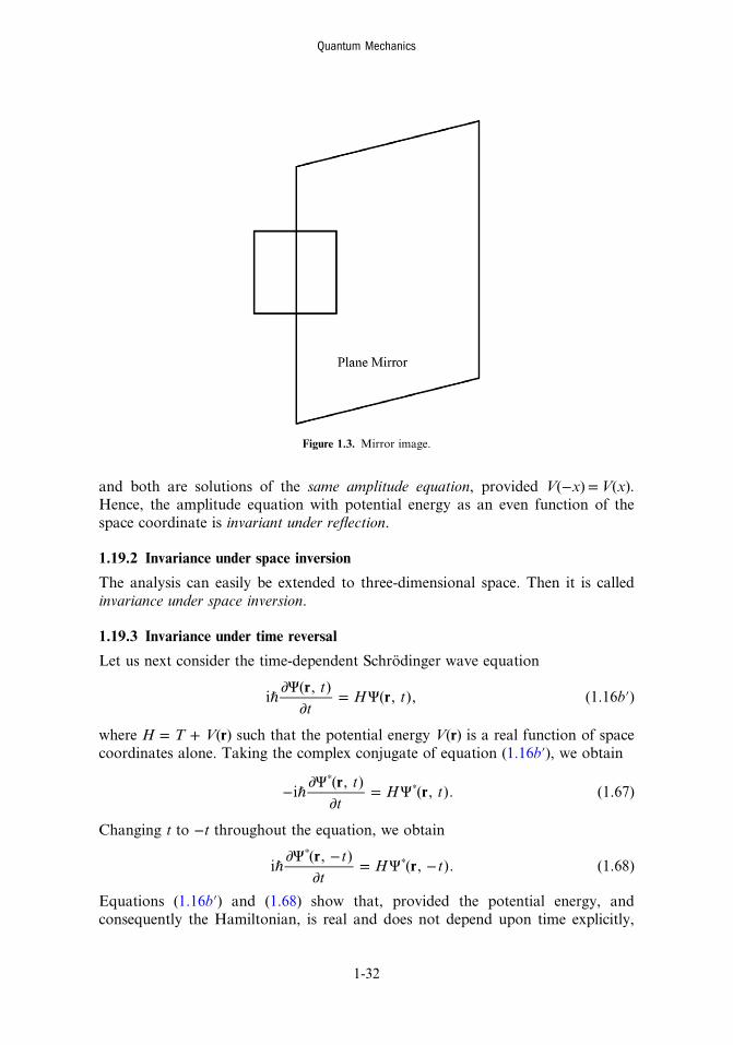
and both are solutions of the same amplitude equation, provided V(−x)=V(x).Hence, the amplitude equation with potential energy as an even function of thespace coordinate is invariant under reflection.

1.19.2 Invariance under space inversion

The analysis can easily be extended to three-dimensional space. Then it is calledinvariance under space inversion.

1.19.3 Invariance under time reversal

Let us next consider the time-dependent Schrödinger wave equation

ℏ ∂Ψ∂

= Ψ ′tt

H t br

ri( , )

( , ), (1.16 )

where H = T + V(r) such that the potential energy V(r) is a real function of spacecoordinates alone. Taking the complex conjugate of equation (1.16b′), we obtain

− ℏ ∂Ψ∂

= Ψ*

*tt

H tr

ri( , )

( , ). (1.67)

Changing t to −t throughout the equation, we obtain

ℏ ∂Ψ −∂

= Ψ −*

*tt

H tr

ri( , )

( , ). (1.68)

Equations (1.16b′) and (1.68) show that, provided the potential energy, andconsequently the Hamiltonian, is real and does not depend upon time explicitly,

Figure 1.3. Mirror image.

Quantum Mechanics

1-32

the wave functions Ψ(r, t) and Ψ*(r, −t) are both solutions of the same time-dependent Schrödinger wave equation. The wave function Ψ*(r, −t) is often calledthe time-reversed solution of the time-dependent Schrödinger wave equation withrespect to Ψ(r, t). The time-dependent Schrödinger wave equation (1.16b′) is said tobe invariant under time reversal. This means that if Ψ(r, t) is a solution of the time-dependent Schrödinger wave equation, then Ψ*(r, −t) is also a solution of the same.

If the system is in a stationary state with definite energy E, then we may write

⎛⎝⎜

⎞⎠⎟ψΨ = −

ℏt

Etr r( , ) ( ) exp

i. (1.69)

Taking the complex conjugate of the above equation, we obtain

⎛⎝⎜

⎞⎠⎟ψΨ =

ℏ* *t

Etr r( , ) ( ) exp

i.

Changing t to −t throughout the equation, we obtain

⎛⎝⎜

⎞⎠⎟ψΨ − = −

ℏ* *t

Etr r( , ) ( ) exp

i. (1.70)

Thus invariance under time reversal implies that, for a stationary state, if ψ(r) is asolution of the amplitude equation, then ψ *(r) is also a solution of the same.

1.20 Concluding remarksWe conclude the first chapter by emphasising that the Schrödinger wave equation isnot a model for the explanation of some experimental results. It is a law of natureand has replaced Newton’s second law of motion for non-relativistic mechanics. Ittherefore provides the foundation for the explanation of mechanical phenomena.However, it is in the form of a differential equation and is not garbed in words. Itspredictions based on a probabilistic interpretation of its solution are consistent withexperiments although sometimes they appear to be at variance with common sense.But what is common sense? It is the knowledge that we gain from our everydayexperience with macroscopic objects. And why do we expect that the microscopicworld would exhibit the same characteristics and behave the same way? If we definecommon sense as the knowledge gained from the behaviour manifested by micro-scopic entities, quantum mechanics becomes fully consistent with common sense!The theory is beautiful and elegant and its achievements are spectacular andfantastic. It has introduced new concepts and changed the pattern of philosophicalinterpretations. We have established the Schrödinger wave equation and interpretedits solutions so as to relate them to physically measurable quantities. Our nextobjective is to apply this theory to solve physical problems in mechanics and duringthis process enhance our understanding of various characteristics of mechanicalphenomena.

Quantum Mechanics

1-33

Additional problems

1.7. Why in the Compton effect is an x-ray photon scattered by an electronwith a change in wavelength while in the photoelectric effect an opticalphoton transfers all its energy to the photoelectron?

1.8. The classical expression for the potential of a linear harmonic oscillatoris 1/2kx2, where k is a constant and x is the displacement of the oscillatorfrom its mean position. Can the Schrödinger amplitude equation be usedfor solving the problem of a linear harmonic oscillator?

1.9. A particle is somewhere on a line of about 7 m in length. Calculate theuncertainty in the measurement of its linear momentum. What con-clusion can be drawn from this result?

1.10. What is the Compton effect? Give its quantum theory and spell out itssignificance.

1.11. What is the energy–time uncertainty relation? If an electron in an atomtakes about −10 8 s to emit radiation in falling from an excited state to alower energy state, calculate the energy uncertainty of such an excitedstate.

1.12. State Heisenberg’s uncertainty relation for position and momentum.Describe an idealised experiment to illustrate the uncertainty relation.

1.13. Show that the probability current density can be expressed as

= − ℏ Ψ ∇Ψ*( )m

j Re i .

1.14. Show that if Ψ is real, then the vector j(r, t) vanishes.

Quantum Mechanics

1-34