Quantum Information Theory forEngineers: An Interpretative

ApproachLecture Notes by C. Jansson

November 6, 2017

1

CONTENTS 2

Contents

1 Introduction 4

2 Experiments 172.1 Historical Remarks . . . . . . . . . . . . . . . . . . . . . . . . . . . 182.2 Numbers . . . . . . . . . . . . . . . . . . . . . . . . . . . . . . . . . 202.3 Polarization of Light . . . . . . . . . . . . . . . . . . . . . . . . . . 262.4 The Law of Malus . . . . . . . . . . . . . . . . . . . . . . . . . . . 302.5 Birefringent Plates . . . . . . . . . . . . . . . . . . . . . . . . . . . 352.6 The Double-Slit Experiment . . . . . . . . . . . . . . . . . . . . . 392.7 Diffraction at Multiple Slits . . . . . . . . . . . . . . . . . . . . . 462.8 Light Reflection . . . . . . . . . . . . . . . . . . . . . . . . . . . . . 522.9 Interferometer . . . . . . . . . . . . . . . . . . . . . . . . . . . . . . 562.10 Delayed Choice Experiments . . . . . . . . . . . . . . . . . . . . . 582.11 Interaction-Free Measurement . . . . . . . . . . . . . . . . . . . . 602.12 Renninger’s Negative-Result Experiment . . . . . . . . . . . . . . 622.13 The EPR Paradox and Bell’s Inequality . . . . . . . . . . . . . . 642.14 Basic Rules of Quantum Mechanics . . . . . . . . . . . . . . . . . 69

3 Introduction to Quantum Information Theory 723.1 Classical Boolean Circuits . . . . . . . . . . . . . . . . . . . . . . 733.2 Reversible Computation . . . . . . . . . . . . . . . . . . . . . . . . 753.3 The Linear Algebra Formalism of Reversible Computation . . . 783.4 Composition of Gates . . . . . . . . . . . . . . . . . . . . . . . . . 833.5 Randomized Computation . . . . . . . . . . . . . . . . . . . . . . 883.6 Quantum Computation . . . . . . . . . . . . . . . . . . . . . . . . 943.7 Quantum Parallelism . . . . . . . . . . . . . . . . . . . . . . . . . 1033.8 Deutsch-Jozsa Algorithm . . . . . . . . . . . . . . . . . . . . . . . 1063.9 No-Cloning Theorem . . . . . . . . . . . . . . . . . . . . . . . . . . 1083.10 Quantum Teleportation . . . . . . . . . . . . . . . . . . . . . . . . 111

4 Unification via Semimodules 1164.1 Preliminaries . . . . . . . . . . . . . . . . . . . . . . . . . . . . . . 1174.2 Base States . . . . . . . . . . . . . . . . . . . . . . . . . . . . . . . 1204.3 Irreversibility and Trinity of Time . . . . . . . . . . . . . . . . . . 1274.4 States . . . . . . . . . . . . . . . . . . . . . . . . . . . . . . . . . . . 1304.5 Some Experiments Revisited . . . . . . . . . . . . . . . . . . . . . 1334.6 Semimodules . . . . . . . . . . . . . . . . . . . . . . . . . . . . . . 1374.7 Change of States . . . . . . . . . . . . . . . . . . . . . . . . . . . . 1404.8 Composition Rules . . . . . . . . . . . . . . . . . . . . . . . . . . . 1414.9 Alternative Bases . . . . . . . . . . . . . . . . . . . . . . . . . . . . 1424.10 Observables . . . . . . . . . . . . . . . . . . . . . . . . . . . . . . . 1464.11 Geometry, Polarization, and Spin . . . . . . . . . . . . . . . . . . 1514.12 Creation and Annihilation Operators . . . . . . . . . . . . . . . . 1594.13 Space and Entanglement . . . . . . . . . . . . . . . . . . . . . . . 1624.14 Clocks and the Lorentz Transform . . . . . . . . . . . . . . . . . 1664.15 Dimension of Space . . . . . . . . . . . . . . . . . . . . . . . . . . 173

CONTENTS 3

4.16 Teleportation: the Experiment . . . . . . . . . . . . . . . . . . . . 1784.17 Uncertainty Principle . . . . . . . . . . . . . . . . . . . . . . . . . 1824.18 Position-Momentum Commutation Relation . . . . . . . . . . . . 187

5 Quantization and Fields 1915.1 Quantization Rules . . . . . . . . . . . . . . . . . . . . . . . . . . . 1925.2 Classical Harmonic Oscillator . . . . . . . . . . . . . . . . . . . . 1955.3 Quantum Harmonic Oscillator . . . . . . . . . . . . . . . . . . . . 1985.4 Matrix Mechanics in Position Representation . . . . . . . . . . . 2065.5 Several Harmonic Oscillators . . . . . . . . . . . . . . . . . . . . . 2095.6 The Oscillator Chain . . . . . . . . . . . . . . . . . . . . . . . . . 2105.7 Quantization of the Chain . . . . . . . . . . . . . . . . . . . . . . 2135.8 The Field as a Continuous Limit . . . . . . . . . . . . . . . . . . 2155.9 Renormalization . . . . . . . . . . . . . . . . . . . . . . . . . . . . 2165.10 Canonical Field Quantization . . . . . . . . . . . . . . . . . . . . 2175.11 Quantization Using Fourier Analysis . . . . . . . . . . . . . . . . 2205.12 Quantization of the Electromagnetic Field . . . . . . . . . . . . . 2245.13 States in QFT . . . . . . . . . . . . . . . . . . . . . . . . . . . . . 2255.14 Conclusions . . . . . . . . . . . . . . . . . . . . . . . . . . . . . . . 226

6 Appendix A: The Theorem of Hurwitz 227

7 Appendix B: Symmetry and Groups 229

8 Appendix C: Keep in Mind 236

Index 242

1 INTRODUCTION 4

1 Introduction

What is the background of this tutorial? These notes comprise lectureson quantum computing and quantum information theory that I taught dur-ing the last ten years for students of electrical engineering. The well-knownand excellently written book of Nielsen and Chuang1 presents an extensivetreatment of various issues and concepts in quantum computing and quantuminformation theory. There are also many other good introductions to quantuminformation theory. So, why these lecture notes?

Physics is known to be a hard science. The physical laws are difficult tointerpret, the meaning of physical quantities and the relationship to reality isvague, and the necessary mathematics requires some effort and capabilities. Inparticular, quantum physics is perhaps recognized as the most difficult subjectin the physics curriculum. It is not only the mathematics used in introductorycourses about quantum theory that causes problems. It is the way of relatingmathematical quantities and concepts, such as superposition, wave functions,spin, or entangled vectors, to the reality we observe.

A major goal of these notes is to present an alternative entranceto quantum information theory that is, hopefully, suitable for stu-dents studying engineering, but perhaps also to people interested inphilosophy of physics.. To my knowledge engineers like machines, experi-mental set-up’s and concrete things, but not so much abstract mathematicalformalisms. These (hopefully enjoyable) notes try to take this mentality intoconsideration by describing many experiments, among them those exhibitingstrange behaviours. Moreover, whenever possible, the mathematical formalismis described in an easily understandable, but sufficiently extensive, manner.

Is quantum mechanics really difficult? In many textbooks the abstractprinciples of quantum mechanics can be found in the following form, or in aslightly modified manner:

• Principle 1 (quantum state space): To every quantum object, quan-tum system, or quantum process a complex vector space (Hilbert space),called the quantum state space, is associated. The complex vectors ∣ψ⟩in this Hilbert space are called quantum states. Two vectors that differonly by a complex multiple represent the same quantum state.

• Principle 2 (observable): To every observable or dynamical variableof a quantum system a Hermitian operator A acting on a quantum statespace is associated. The only possible results of a measurement are theeigenvalues of this Hermitian operator.

• Principle 3 (measurement): If an eigenvalue of an observable A ismeasured, then the state of the quantum system jumps to an eigenvectorcorresponding to this eigenvalue. Quantum mechanics is a probabilitytheory. The expectation value of an observable A for a quantum systemin quantum state ∣ξ⟩ is ⟨ξ∣A∣ξ⟩.

1Nielsen, Chuang [2010]

1 INTRODUCTION 5

• Principle 4 (Born’s probability rule): The transition probability fora given normalized quantum state ∣ψ⟩ jumping to any normalized state∣φ⟩ is the squared absolute value ∣⟨ψ∣φ⟩∣2.

• Principle 5 (time evolution): The evolution of state vectors of anisolated quantum system is unitary with respect to time.

• Principle 6 (composition rule): Two or more quantum systems arerepresented by the tensor product of the corresponding quantum statespaces.

Basically, Principle 1 shows the arena for quantum mechanics. Principles 2,3, and 4 state that quantum mechanics is a linear stochastic theory. Principle 5says that the dynamics of isolated quantum systems is a unitary deterministicevolution, and in particular a reversible process. Principles 3 and 5 show theparadox that quantum mechanics is governed by two dynamics: the irreversiblestate function collapse, where the superposition of eigenstates reduces to asingle eigenstate by measurement or observation, whereas the other dynamicsis a continuous, deterministic and unitary transformation. Principle 6 tells usthat different state spaces of quantum systems are combined to a compositesystem via the tensor product.

Representative for many other physicists we cite three well-known scien-tists. They write about these apparently weird quantum principles:

Nothing could be more arid than the principles of quantum me-chanics. Its concepts and laws are cast in a blunt, inescapable math-ematical form, without a trace of anything intuitive, a total absenceof the obviousness we see in the things around us. And yet, thistheory penetrates reality to a depth our senses cannot take us. Itslaws are universal, and they rule over the world of objects so famil-iar to us. We, who inhabit this world, cannot make our own visionprevail over those arrogant laws, whose concepts seem to flow froman order higher than the one inspired by the things we can touch,see, and say with ordinary words. Omnes2 1999

Might I say immediately, so that you know where I really intendto go, that we always have had (secret, secret, close the doors!) wealways have had a great deal of difficulty in understanding the worldview that quantum mechanics represents. Feynman3 1982

Those who are not shocked when they first come across quantummechanics cannot possibly have understood it. Attributed to Bohr

Schrodinger cats, Wigner’s friend, many worlds and many minds in non-relativistic quantum mechanics, and moreover time dilation, length contrac-tion, the lack of simultaneity, worm-holes, non-causality, and several other

2Omnes [1999, page 163]3Feynman [1982, page 471]

1 INTRODUCTION 6

paradoxes in relativistic quantum mechanics do not make things easier (seeFigures 1, 24, 3, and 45).

Because the fundamental parts of physics are quantum theory and thetheory of relativity, not surprisingly many physicists view their science as acollection of purely mathematical concepts without relation to reality. Forinstance, the positivist and cosmologist Tegmark writes:

I advocate an extreme ”shut-up-and-calculate“ approach to physics,where our external physical reality is assumed to be purely math-ematical. This brief essay motivates this ”it’s all just equation“assumption and discusses its implications. Tegmark6 2007

We shall spend a lot of time in finding out, however, that the previousprinciples are actually very intuitive and reasonable, and can be deduced fromeasily comprehensible fundamental rules. This road starts by justifying the useof complex numbers and ends by discussing some aspects of time. Althoughquantum mechanics seems to be a rather bizarre description of reality, weshould keep in mind that it is known as our most fundamental and successfulphysical theory ever which is irreducible and random. Their predictions havebeen tested to an unprecedented accuracy.'

&

$

%

ψ = 12 left 1

2 right

Figure 1: To show the strange behavior of quantum particles, in some booksthe quantum skier is used who goes both ways at once. They remark thatalthough we do not observe such phenomena, they happen in the quantumworld.

4Dhatfield [2008]5Schirm [2011]6Tegmark [2007]

1 INTRODUCTION 7

Figure 2: Schrodinger’s cat is a famous illustration of the principles of super-position and entanglement in quantum theory, proposed by Erwin Schrodingerin 1935. Originally, his intention for this cat-killing box was to discredit non-intuitive implications of quantum mechanics.

#

"

!ψ  

12

Figure 3: Superposition of alive and dead.

What is physics today? What is truth in physics? The expression”physics“ comes from the ancient Greeks and means ”knowledge of nature”.This implies that we are and should be interested in true information about ourworld. What is true? This is a difficult question, and in fact von Weizsacker7

starts his book about the structure of physics with the question: What is thetruth of physics?

On the gravestone of the well-known Russian mathematician, physicist,and philosopher Danilovich Aleksandrov (1912 - 1999) one finds the graving8:”The truth is the only thing, which is worthy of our worshipping”. It shouldget the alarm bells ringing that the famous mathematician and physicist RogerPenrose, author of the excellent book ”The Road to Reality, A complete Guideto the Laws of the Universe“ said in an interview:

Physics is wrong, from string theory to quantum mechanics.Roger Penrose, 2009, DISCOVER

In 2010 he said farewell to our celebrated ”big-bang theory“ and proposedthe old ”steady-state model“:

The scheme that I am now arguing for here is indeed unortho-dox, yet it is based on geometrical and physical ideas which are very

7von Weizsacker [1988]8Gessen [2013, page 151]

1 INTRODUCTION 8

Figure 4: The many worlds theory claims that the universe splits into distinctworlds, in order to have only one unitary dynamics. This would imply theaccommodation of each possible outcome.

soundly based. Although something entirely different, this proposalturns out to have strong echoes of the old steady-state model! Pen-rose9

By the way, the widely glorified and seemingly experimentally verified mes-sage about the age of our universe would be wrong when believing Penrose.On the contrary, in Wikipedia, and not only there, you find the confirmationof the age of our universe in high precision:

In physical cosmology, the age of the universe is the time elapsedsince the Big Bang. The best measurement of the age of the uni-verse is 13.798 pm 0.037 billion years within the Lambda-CDM con-cordance model. The uncertainty of 37 million years has been ob-tained by the agreement of a number of scientific research projects,such as microwave background radiation measurements by the Plancksatellite, the Wilkinson Microwave Anisotropy Probe and other probes.Wikipedia, August 2012

All this becomes even more strange when knowing the Wheeler DeWittequation: This field equation is one approach to the famous problem of quan-tum gravity, and turns out to be timeless. No time, no age of the universe?However, already Landau mentioned

Cosmologists are often in error, but never in doubt. Lev Lan-dau10

So who is right? Perhaps such contradictory statements support thewell-known rule in physics:

9Penrose [2010, Preface]10http://yquotes.com/quotes/lev-davidovich-landau/

1 INTRODUCTION 9

The theory determines what we observe and measure.

This rule may point to circular reasoning. Measurements confirm the the-ory, which then determine the measurement results.

Among physicists there is no fundamental disagreement on how to usemathematical formalisms for practical applications. However, there are deepdifferences in the understanding and meaning of physical theories, in particular,of quantum theory but even so in the theory of relativity. For instance, almostall ancient famous scientists, among them Descartes, Newton, Gauss, Riemann,Lord Kelvin, and Maxwell, investigated different mechanical models of ”ether”.Actually, Maxwell derived his equations from a purely mechanical ether model,see the cover sheet of these notes. Einstein finished the ether in a lone hand.The Nobel honoree in physics Laughlin writes about ether in contemporarytheoretical physics:

It is ironic that Einstein’s most creative work, the general the-ory of relativity, should boil down to conceptualizing space as amedium when his original premise [in special relativity] was that nosuch medium existed [..] The word ’ether’ has extremely negativeconnotations in theoretical physics because of its past associationwith opposition to relativity. This is unfortunate [...] Relativityactually says nothing about the existence or nonexistence of mat-ter pervading the universe, only that any such matter must haverelativistic symmetry. [..] Subsequent studies with large particleaccelerators have now led us to understand that space is more likea piece of window glass than ideal Newtonian emptiness. It is filledwith ’stuff’ that is normally transparent but can be made visible byhitting it sufficiently hard to knock out a part. The modern conceptof the vacuum of space, confirmed every day by experiment, is arelativistic ether. But we do not call it this because it is taboo.Laughlin11

Apparently, this taboo indicates that also many scientists behave politicallycorrect, perhaps also in spite of a clearer understanding. Consequently, thetruth content of physical theories is very controversial and doubtful.

In particular, for engineers interested in these aspects, we mention thatthere are plenty of books and articles with a critical attitude that clearly pointout shortcomings, critics and incredible models of the present physics12. Thesebooks contain many further references. The history of science clearly demon-strates that doubtfulness is the chief impelling force, not faith. Unfortunately,as far as I know, almost all time in the education at schools and universities isspent with believing and learning, not casting doubt on the theories. Perhapsthe literature mentioned above might help.

What can we understand? What should students understand?Understanding is a complex psychological process and hard to describe in an

11Laughlin [2005, pp. 120–121]12 Herbert [1985], Mirman [2001, 2006], Omnes [1999], Rothmann [2012], Selleri [1990],

Sheldrake [2013], Smolin [2006, 2013], Unzicker [2010, 2012, 2013]

1 INTRODUCTION 10

abstract form. Serious scientists as well as engaged students have frequentlydoubts about the proper understanding of their science. In particular, manystudents have profound doubts whether they have understood the lecturesthey have heard, or the textbooks they have read. Partially, these doubtsare well-founded, but sometimes these doubts arise because certain scientificstatements are fired from teachers or other students as simple or trivial. Letus consider three well-known examples.

One seemingly very simple statement is the principle of inertia, alreadydescribed in physics courses in school. Is it in fact simple? Do we understandit? There is a nice story in YouTube13 where Richard Feynman talks abouthis father:

My father taught me to notice things. One day I was playing withan express wagon, a little wagon with a railing around it. It had aball in it, and when I pulled the wagon I noticed something aboutthe way the ball moved. I went to my father and said,”Say, pop,I noticed something. When I pull the wagon, the ball rolls to theback of the wagon. And when I am pulling it along and I suddenlystop, the ball rolls to the front of the wagon. Why is that? ...

”That, nobody knows“, he said. ”The general principle is thatthings which are moving tend to keep on moving, and things whichare standing still tend to stand still, unless you push them hard.This tendency is called inertia, but nobody knows why it’s true.“

Feynman was proud of the way he was educated by his father, who gave himthe difference between knowing the name of something and under-standing something. That the principle of inertia is in fact a deep physicalproblem and paradox is only rarely mentioned. An exception is the book ofvon Weizsacker14 who writes:

The law of inertia, which empirically enforces the occurrence ofsecond derivatives in the equation of motion, is fundamental forclassical mechanics. It, however, represents a causal paradox. Aris-totle understood motion as a change of state, and thus force as thecause of motion. In classical mechanics, however, inertial motionis just the motion without any forces acting. In the seventeenthcentury one still felt the paradox therein; Descartes and, followinghim, Newton defined the state of a body in terms of its velocitysuch that only acceleration was seen as a change of state. But thisis inconsistent, as two bodies with the same velocity but at differ-ent locations are in different states, as correctly put by the moderndescription in phase space; and during inertial motion the point inphase space varies. If one wants to think causally in a consistentway, one must radicalize Mach’s ideas and interpret the inertialmotion as being caused by the universe (the distant masses). This

13 https://www.youtube.com/watch?v=Zjm8JeDKvdc14von Weizsacker [2006, p. 29]

1 INTRODUCTION 11

I have attempted in the ur theory, but now I doubt whether this isan adequate formulation.

Another example is the theory of special relativity. It is widely accepted,widely tested, and widely understood, although it is a weird theory containingstrange interpretations such as time dilation, Lorentz contraction, velocity ad-dition, the relativity of simultaneity, moving frames, observers and many othermysterious quantities. However, the mathematics behind is simple since it re-quires only matrix-vector operations. But nobody should be shamed to admithaving difficulties with this theory. Even their excellent co-founders Lorentzand Poincare seemed not to have understood relativity, as Pais15 writes:

In later years all three man, Einstein, Lorentz, and Poincare, re-acted to the special theory of relativity in ways which arouse cu-riosity. Why on the whole, was Einstein so reticent to acknowl-edge the influence of the Michelson-Morley experiment on his think-ing? Why could Lorentz never quite let go of the aether? Why didPoincare never understand special relativity?

The book of Pais is very suitable for reading, contains many details aboutthe history of the theory of relativity, and gives a very good insight into thethinking of their founders.

The third example is the well-known Monty Hall problem, a rather simpleprobabilistic problem, named after Monty Hall who presented it the first timein 1975. Even Erdos, one of the greatest experts in number and probabilitytheory, could not solve this puzzle, and was unconvinced until a computersimulation, confirming the predicted result, was shown to him, see Vazsonyi16.

There are various other examples in science, and sometimes this has un-pleasant consequences. Griffiths17 writes about Bohr:

It is interesting to note that Bohr was an outspoken critic ofEinstein’s light quantum (prior to 1924), that he mercilessly de-nounced Schrodinger’s equation, discouraged Dirac’s work on therelativistic electron theory (telling him, incorrectly, that Klein andGordon had already succeeded), opposed Pauli’s introduction of theneutrino, ridiculed Yukawa’s theory of the meson, and disparagedFeynman’s approach to quantum electrodynamics. Great scientistsdo not always have good judgment - especially when it concernsother people’s work - but Bohr must hold the all-time record.

When we don’t impute some kind of badness, it seems that Bohr had difficultiesto understand what other physicists published in his area of expertise.

My advice to students is: take the liberty to have doubts, for the momentskip the things you do not understand, and do not fear to make errors. Nobodyis perfect, and science is not error-free, as we have already remarked.

Which problems may occur when teaching quantum physics?

15Pais [2005, p. 164]16Vazsonyi [1999, pp. 17–19]17Griffiths [2004, p. 23]

1 INTRODUCTION 12

What is weird is not nature, not physics, not the universe, but theobsession of so many physicists with demonstrating their inabilityto understand physics by regarding nature as spooky. Mirman18

For many students quantum physics is a hard science. In particular, if theyare educated by the well-known ”Shut up and calculate“ approach, physics maybecome a very dubious pleasure, not really funny, and perhaps only suitable toearn some money, on a later date. If in textbooks classical concepts are usedto generate contradictions and paradoxes such that quantum physics seems tobe magical, then confusion arises (see Figures 1, 2, 3, and 4). Magic may begood for entertainment, but it is not really helpful for students to understandthe physical concepts. Also for philosophers, interested in quantum physicsand broader questions about nature, ontology, and human knowledge, magicis a bad adviser.

There is no experimental evidence whatsoever to support such magic, butnaive pictures. Quantum paradoxes originate solely from erroneous interpreta-tions of quantum theory. Only pseudo-realistic philosophies together with themisuse of the underlying mathematical concepts leads to paradoxical results.

Here, we try to avoid such magical descriptions, and instead try to maintaina more critical attitude:

If a man will begin with certainties, he shall end in doubts; Butif he will be content to begin with doubts, he shall end in certainties.

Francis Bacon, Advancement of Learning.

What are the major differences to other textbooks on quantuminformation and quantum computation? In this lecture notes there aresome interpretations and models that are different, or perhaps some may benew, when comparing with other books.

This work contains many things which are new and interest-ing. Unfortunately, everything that is new is not interesting, andeverything which is interesting, is not new. Lev Landau19

Also on the danger that Landau is right, I would like to mention the followingpoints:

• We support the understanding of this difficult subject by numerousexperiments, and use the ability of the engineer to think in terms ofmachines. This gives an experimental entrance to quantum in-formation theory. The picture on the title page supports this pointof view. It displays Maxwell and his mechanical notion of his famousequations describing electromagnetism.

• We argue why the field of complex numbers C is the universalset of numbers in science. In particular, it can be shown that clas-sical mechanics and quantum mechanics can be embedded in the same

18Mirman [2001, p. 197]19http://yquotes.com/quotes/lev-davidovich-landau/

1 INTRODUCTION 13

mathematical framework when working with complex numbers; the realdynamical variables of classical mechanics are just the quantum mechan-ical average values of Hermitian operators. Consequently, classical me-chanics works with real numbers and quantum mechanics with complexnumbers.

• We explain the central topics of quantum mechanics and quantum com-putation only with the help of the simple and natural Dirac-Feynmanrules, avoiding strange quantum mechanical principles whenever possi-ble.

• Only a minimal mathematical formalism is necessary. Large partsof these notes can be already taught in school.

• These lecture notes are perhaps exceptional in a unified treatment ofclassical, random and quantum computation. In particular, quantumcomputation as well as random computation are described as a sim-ple and natural mathematical modification of classical reversiblecomputation, and in this way it is easy to understand for studentshaving some knowledge in classical computation.

• We avoid magic pictures and imaginations, many paradoxes, anddescribe quantum computation as a linear stochastic process.

• We point out at various places the conflict between quantum me-chanics and the theory of relativity.

• We treat quantum mechanics, classical probability theory and classi-cal mechanics within the same mathematical framework which is basedon semimodules. We obtain unified definitions of states, observ-ables and evolution operators that do not depend on the spe-cific physical theory. In particular, we introduce in our frameworkwhich describes various physical models the useful concepts number rep-resentations, register representations, and vector representations.

• We show that the apparent inconsistency between classical probabilitytheory and quantum mechanics, as seen in slit experiments or Bell’s in-equality, can be resolved when carefully looking at the notion of outcomesin the classical theory and the possibilities in quantum mechanics.

• We derive the mathematical framework of quantum two-state systemsand an uncertainty principle using only simple geometry at a macro-scopic level. Microscopic properties like spin or polarization are notrequired.

• In physics time t is treated as an external background parameter. Weavoid this concept, and use time only in terms of three modes, namelythe trinity future, present, and past. Consequently spacetime vanishes.But we present an alternative approach to the Lorentz transform, thekey to the theory of relativity.

1 INTRODUCTION 14

• We explain the two fundamental problems in quantum theory, namelythe meaning of superposition and entanglement, in terms of our timetrinity.

• We investigate and try to explain the famous riddle of inertia.

• A fundamental assumption in physical theories is the dimension of theunderlying space. In most cases this is the (3+1)-dimensional space-time. However, there are other well-known theories that use other dimen-sions, among them the 11-dimensional string theory or the 5-dimensionalKaluza-Klein theory. From the point of view of information theory weinvestigate in which dimensions a physical theory can be reasonable. Sur-prisingly, it turns out that, in some well-known theories, the underlyingspaces do not satisfy even simple geometrical properties.

• We discuss very critically to what extent teleportation takes place in theexperimental set-up.

• We give an interpretation of Heisenberg’s uncertainty principle that isnot common.

Which prerequisites are necessary? The following lecture notes goback to the quantum computation courses I taught during the last years. Theyare not written for experts or for brilliant students. They are mainly writtenfor those readers who find the subject difficult. The text focuses on the ma-jor concepts of quantum information theory, while keeping mathematics toan indispensable minimum. We assume only a knowledge of the elementaryfacts of linear algebra, such as matrix-vector multiplication or eigenvalues andeigenvectors.

We abandon a separate section about linear algebra, since almost all text-books about quantum mechanics or quantum computing contain such a section.In the afore mentioned book of Nielsen and Chuang20 a very nice presentationis given in Section 2.1. Other descriptions, for instance, can be found in thebooks of Kaye, Laflamme, and Mosca21, and in Plenio22.

It should be clear that reading these notes only is not a good way to learnquantum information theory, especially without having any prior knowledge.I recommend some additional textbooks for students and engineers that arewilling to broaden their knowledge about physics. Firstly, there are two booksof the series The Theoretical Minimum: What you Need to Know to StartDoing Physics. The first one is written by Leonard Susskind and GeorgeHrabovsky23 and covers classical mechanics, the core of education in physics.The second one by Leonard Susskind and Art Friedman24 explains quantummechanics and its relationship to classical mechanics. Both volumes containthe necessary mathematical definitions, theorems, and prerequisites. They are

20Nielsen, Chuang [2010]21Kaye et al. [2007, Chapter 2, pp. 799–800]22Plenio [2002, Chapter 1]23Susskind [2013]24Susskind [2014]

1 INTRODUCTION 15

based on Susskind’s popular Stanford education courses that can be foundin YouTube. Susskind, Hrabovsky and Friedman provide a toolkit for non-advanced students to learn physics at their own pace.

For a deeper understanding of physics, namely classical theories as wellas quantum theory, we emphasize the older, but unforgettable, lecture notesof Feynman25. In contrast to many textbooks that teach mainly physical andmathematical formalisms in same compact manner, these notes explain physicsfrom the very beginning by looking at many experiments and observations. It’sjust the way of how to think in physics.

Finally, for interested readers some further excellently written textbooksare mentioned26.

What about the contents? I tried to write a small book guided byLandau’s experience:

From thick books one can not learn anything new. A thick bookis a cemetery where antiquated ideas are laid to rest. Lev Landau27

The major goal of Section 2 of these lecture notes, is an elaborate presen-tation of some fundamental, strange sounding experiments of physics. Theseinclude experiments with photons, their polarization, reflection, multiple slitexperiments, interaction free measurement, and delayed choice experiments,as well as Bell’s inequality. These experiments are not only depicted, they areinvestigated using the Dirac-Feynman probability rules. Moreover, it is shownthat these rules are almost inescapable and natural, leading to a descriptionof quantum theory as a stochastic process with complex amplitudes.

In Section 3 the fundamental concepts of quantum computing and quan-tum information are described, including the similarity and differences betweenreversible classical computation, random computation, and quantum compu-tation. Moreover, quantum teleportation as well as applications of quantumparallelism are considered.

In Section 4 we present some fundamental concepts and foundations ofquantum theory. In particular, we try to give precise and unified definitions ofbase states, states, observables, compositions of systems, and transformationsbetween systems. We replace the concept of an external time parameter bythe trinity future, present and past and show its consequences. We develop analternative to the theory of relativity.

In Section 5 we discuss detailed the fundamental concept of canonical quan-tization, known as the process of constraining continuous quantities to discreteones. In particular, an introduction to quantum field theory is presented, in-cluding the quantization of the electromagnetic field.

Finally, an appendix is attached containing the theorem of Hurwitz, a veryshort introduction to symmetry and groups, and some ”Keep in minds”.

These lecture notes certainly do not meet the standard of a textbook, bothbecause of structure and language. They are only an extended version of my

25Feynman Lectures [1963]26Greiner [2005], Omnes [1994], Penrose [2005], Weinberg [2013], Zetteli [2009]27http://yquotes.com/quotes/lev-davidovich-landau/

1 INTRODUCTION 16

lectures. It was my intention to question certain interpretations of quantuminformation theory and physics, and to stimulate thought.

Feedback This text is free to download from the internet

• http://www.ti3.tuhh.de/jansson/.

I am deeply grateful for corrections, comments, and suggestions:

• jansson@tuhh.de.

Acknowledgements I am grateful to a number of colleagues and students.In particular, I wish to thank Ulrike Schneider for her assistance in prepar-ing this lecture notes, including graphics, tables, much of the latex code, andreading. I wish to thank Kai Torben Ohlhus and David Sills for their criticalreading of the manuscript, their feedback, and their suggestions. It is my plea-sure to thank Fritz Mayer-Lindenberg. Many years ago I shared the lectureson quantum computation with him. My special thanks goes to Frerich Keilfor many valuable and friendly conversations and hints regarding the litera-ture. These notes have been tested especially in my last course 2016. I amgrateful to some of the students for comments. In particular, I would like tomention Max Ansorge, Antonio Attimonelli, Annika Evers, Georg Felbinger,Lennart Manthey, Hendrik Meyer zum Felde, Hendrik Preuß, Nicolas Riebeseland Anselm Jonas Scholl.

Hamburg, Germany, August 2017Christian Jansson

2 EXPERIMENTS 17

2 Experiments

The aim of this section is to give students an impression of quantum mechanicsby describing and looking closely at several experiments. We present quantummechanics from the point of view of probability theory and stochastic processes.We do this in a very elementary way, and demonstrate the need of a type ofprobability that does not satisfy the rules of Kolmogorov’s classical probabilitytheory, but requires squared magnitudes of complex numbers.

An understanding of nature and particularly physics can only be obtainedwhen putting questions in the form of experiments. All of our knowledgeabout nature can be expressed in terms of a sequence of binary YES or NOquestions, namely bits. They lead in a natural way to two-state systems. Two-state systems are the fundamental elements in quantum information theory.

We consider at the beginning the polarization of light which is one exampleof a two-state system. Other examples are the double-slit experiment and theMach-Zehnder interferometer. Not surprisingly, it turns out that almost allfundamental principles of quantum mechanics can be derived on the basis oftwo-state systems.

This chapter is written in a manner such that also pupils of a grammarschool, taught complex numbers, can understand the mathematical descriptionof these quantum experiments. Even elementary concepts of matrix algebraare not used. Only the addition and multiplication of numbers is required.

2 EXPERIMENTS 18

2.1 Historical Remarks

The following remarks serve only as a rough orientation, and can be skippedin a first reading.

The basic frameworks of quantum mechanics, quantum field theory, andquantum information theory are presented in books frequently as a collectionof postulates. These postulates and their consequences seem to be non-intuitiveand mysterious. One reason for some paradoxes in quantum mechanics maybe that in textbooks physics is described from a historical point of view, withless emphasis on reasoning or logic.

Schrodinger, 1926, introduced the concept of a wave function satisfyinghis linear partial differential equation in order to describe the motion of elec-trons in atoms. Almost at the same time Heisenberg introduced a seeminglycompletely different model of time-dependent operators acting on so-called”quantum states“, the latter are time-independent. Later, both models wereshown to be mathematical equivalent.

Based on Schrodinger’s wave equation, in many textbooks a strange prop-erty of quantum mechanics, namely the wave-particle duality, is often verbal-ized. This duality says that microscopic particles, like photons, electrons oratoms, do neither behave as a point-particle nor as a wave, but as both. Itdepends on the experiment whether the microscopic object shows particle-likeproperties or wave-like properties.

The most frequently used experiment for depicting this wave-particle na-ture is the famous double-slit experiment, which we shall consider later indetail. If both slits are open a particle shows an interference property as weknow from waves. But, if it is clear through which slit the particle goes, theinterference disappears and a typical point-like statistic is observed.

Dirac suggested in 1932 a third formalism that avoids wave-particle dual-ity. It was forgotten until 1941 when Feynman elaborated this idea. Now itis known as the path integral formalism or sum over history formalism. Thisformalism is described excellently in the Feynman lectures on physics, Volume3, as well as in Feynman’s famous book “QED the strange theory of matterand light”, 1985, where he presents our best physical theory, quantum electro-dynamics. This theory describes all phenomena of the physical world,except gravitation and radioactive phenomena28.

The fundamental idea of Feynman’s theory is so simple that its far-reachingconsequences are astonishing:

In this formalism complex numbers, called ”probability ampli-tudes“ are assigned to elementary events, paths, or other possibili-ties. These amplitudes are added for mutually exclusive events andare multiplied for independent events.

The relation between classical probabilities and probability am-plitudes is established by Born’s rule, 1926: the squared magni-tudes of the amplitudes are the probabilities. In fact, this ideamight go back to Malus 1810, who used squared magnitudes fordescribing some optical experiments.

28Feynman [1985, page 8]

2 EXPERIMENTS 19

The addition and multiplication rule in quantum theory is similar to classi-cal probability theory formalized by Kolmogorov in 1933. But in the classicaltheory we operate not with complex numbers. Instead only non-negative realnumbers are used.

Summing up numbers along any events or paths is actually integrating,hence the word ”path integral formalism”. The path integral can be viewedas a function of the final event. This function satisfies Schrodinger’s equa-tion, and thus Schrodinger’s and Heisenberg’s formalisms can be derived fromFeynman’s theory. The important advantage of Feynman’s approach is its niceinterpretation as a linear stochastic process. It is rather easily understandablewith a rudimentary knowledge of classical probability theory, and seems notto be mysterious. However, for many practical problems the Heisenberg andSchrodinger formalisms are more appropriate from a computational point ofview.

Keep in mind: Feynman’s path integral theory impliesSchrodinger’s as well as Heisenberg’s formalism. It forms the basisof quantum electrodynamics, our best physical theory.

In this chapter, we try to get a feeling for the world of quantum mechanics aswell as for the path integral formalism by looking closely at several astonishingexperiments. A key point is the visualization of numbers as little arrows. Weshall see that many physical features can be understood quite simply whendoing this.

2 EXPERIMENTS 20

2.2 Numbers

Physical theories deal with systems of numbers. In probability theory non-negative numbers are used, in classical mechanics real numbers are used, andquantum mechanics works with complex numbers.

In particular, it can be shown that classical mechanics and quantum me-chanics can be embedded in the same mathematical framework when workingwith complex numbers; the real dynamical variables of classical mechanics arejust the quantum mechanical average values of Hermitian operators29.

Since all physical models are formulated basically with the set of complexnumbers or specific subsets, it raises many questions. Are there other sets ofnumbers, such as quaternions or octonions, that might describe physics andnature in a much better way than the numbers mentioned above? What do wecall a number? Why is quantum mechanics, from most physicists viewed as thefundamental physical theory, based on the field of complex numbers? Wouldother number systems perhaps give new insights? Are there any propertiesthat are common to all number systems? Of course, such basic questions arenot easy to answer. In other words, if we go very deeply into these questionsthey might become unanswerable. However, some clarifications can be given.

The idea of numbers starts with simple counting, namely with integers. In-tegers can be visualized on a line as multiples of a unit arrow, which we denoteby 1. Integers can be added and multiplied. With regard to arrows, they areadded by attaching the head of one arrow to the tail of another, yielding afinal arrow from the tail of the first to the head of the last one. The multipli-cation of integers is defined as the addition in succession. The advantage ofvisualizing numbers as arrows is an action-oriented view of numbers, and givesabstract symbols a pictorial form, well-suited for engineering education. Both,addition and multiplication, have the fundamental property that the result ofthe operation does not depend on the order of the integers. These operationsare commutative as well as associative.

Already the Greeks generalized the concept of integers to rational numbers.They represented numbers as transformations of a unit arrow 1. The transfor-mations are expansion and shrinkage, leading to the positive rational numbers.The well-known addition and multiplication of rational numbers can simply bevisualized in terms of arrows. Addition is the same operation as for integers.Multiplication, in terms of arrows is as follows: we multiply 1/4 with 1/3 byshrinking the unit arrow 1 to 1/4, and then shrinking the resulting arrow by1/3. As for integers the rational operations are commutative. The positive ra-tional numbers are extended with the invention of zero and negative numbers,leading to a representation on the axis of real numbers. The negative numberscorrespond to arrows that are rotated by the angle π. In particular, the unitarrow −1 is obtained by rotating 1. The well-known extended operations forrational numbers can be simply realized in terms of arrows as above, and theyare commutative and associative. The concept of rational numbers was im-proved by inventing real numbers, that is, numbers or arrows on the real axisthat cannot be represented by rational numbers. The real addition and real

29Strocchi [1966]

2 EXPERIMENTS 21

multiplication remain commutative and associative. All real numbers, say xand y, positive or negative, have a length, also called magnitude that satisfiesthe equation

∣xy∣2 = ∣x∣2∣y∣2. (1)

In science it is customary to speak of a number system, if it shares thefollowing basic indispensable properties:

Numbers have a magnitude satisfying (1). They can be added andmultiplied, where both operations are associative and commu-tative. Moreover, they have a neutral element 0 for additionand a neutral element 1 for multiplication.

The sets of numbers mentioned above satisfy these properties. Moreover, thenumbers as well as their operations can be represented as arrows and geometri-cal operations with these arrows, respectively. The sets of natural numbers N,integers Z, rational numbers Q, real non-negative numbers R+, real numbersR, and complex numbers C are number systems. The set of purely imaginarynumbers is not a number system, since the product of two imaginary numbersis a real number.

It seems that the process of constructing new systems of numbers, startingwith the natural numbers, can be continued ad infinitum. So let’s continue.What can we do with our arrows, in order to extend the field of real numbers.For obtaining negative numbers, we have rotated the positive numbers by theangle π. This suggests to rotate with an arbitrary angle in a plane, leading toan extension of the real line to a set of arrows living in a plane. If we rotatethe unit arrow 1 with angle π/2, then we get an arrow which we call i. Sincerotating with π is the same as rotating two times with π/2, we obtain i2 = −1,provided we define the multiplication appropriately in terms of a rotation. Infact, this idea leads to the field of complex numbers.

Because of its importance, we give here a very short introduction to complexnumbers. There are two ways to think about complex numbers. Firstly, thecustomary algebraic point of view is to describe complex numbers as two-dimensional vectors

z = (x, y) = x ⋅ 1 + y ⋅ i, (2)

where both, x and y, are real numbers. Usually, the unit 1 and the dots areomitted. These vectors represent our arrows in the plane. The first componentx is called the real part, and the second component y is called the imaginarypart of z. Two complex numbers can be added

z1 + z2 = (x1 + x2, y1 + y2), (3)

and multiplied

z1z2 = (x1x2 − y1y2, x1y2 + y1x2). (4)

Obviously, the addition is related to the addition of arrows, where we attachthe head of one arrow to the tail of the other, see Figure 5. From formula (4)

2 EXPERIMENTS 22

'

&

$

%

iy

i

1 x

z1

z2

z1 + z2

Figure 5: Addition of complex numbers z1 + z2 = (x1 + x2) + i(y1 + y2) is com-mutative.

it is not clear that the multiplication corresponds to a rotation. This pointwill be explained below.

Both operations define a commutative field, where natural numbers, frac-tions and real numbers can be viewed as subsets of the field of complex num-bers. The difference to the previous systems of numbers is the existence ofcomplex numbers, living in a plane. Take for instance i = (0,1). Then themultiplication rule (4) yields i2 = (−1,0) which can be identified with the neg-ative number −1. In other words, squares of complex numbers can be negative.

The complex conjugate of z is denoted by

z∗ = x − iy, (5)

and is obtained by flipping z over the horizontally axis, see Figure 6.It is important to notice that the complex conjugate star operator is defined

for any number contained in the field of complex numbers. Hence, the complexconjugate is well-defined for integers, positive numbers, rational numbers orreal numbers. In these cases the star operator is just the identity.

The squared magnitude of a complex number is the product with its com-plex conjugate:

∣z∣2 = zz∗ = x2 + y2. (6)

Any complex number z can be written, using the famous Euler formula

cosφ + i sinφ = eiφ, (7)

2 EXPERIMENTS 23

'

&

$

%

iy

x

z = x+iy = rei

|z| = r

z* = x-iy = re-i

rei(

Figure 6: Complex and conjugate complex numbers z and z∗, respectively.

in its polar form

z = ∣z∣eiφ, (8)

where both, the magnitude ∣z∣ and the phase angle φ are real non-negativenumbers. In other words, any complex number is an arrow with a non-negativemagnitude and a generalized sign, called the phase. The phase can be viewedas a rotational operator.

Given two complex numbers z1 = ∣z1∣eiφ1 and z2 = ∣z2∣eiφ2 , we easily obtainwith some trigonometric identities the multiplication rule

z1z2 = ∣z1∣ ∣z2∣ei(φ1+φ2). (9)

Hence, the magnitudes of the complex numbers are multiplied, and the anglesare added to yield the polar form of the product. In particular, the multipli-cation corresponds to a stretching operator and a rotation, see Figure 7.

Complex numbers are an extension of the field of real numbers, since theycontain all real numbers and there is no real number which is the squareroot of −1. Moreover, rewriting a complex number as a pair of real numbers,namely the real and the imaginary part, the field of complex numbers canbe viewed as a real vector space, that is, a set of vectors satisfying the twofundamental rules: we can add them, and we can multiply them with a realnumber, the latter is called scalar multiplication. But this does not mean thatthe field of complex numbers is algebraically isomorphic to an appropriate two-dimensional real space.30 The fundamental complex operations make this set

30For instance, the special unitary group SU(2), consisting of the two-dimensional uni-tary matrices with determinant equal to one, is not homeomorphic to the group SO(4),consisting of the real orthogonal matrices with determinant equal to one, as it might beexpected if complex numbers are just two-dimensional real vectors. It turns out that SU(2)is homeomorphic to SO(3).

2 EXPERIMENTS 24

'

&

$

%

iy

i

1 x

z1

z2

z1 · z2

12

1+2

Figure 7: Multiplication of complex numbers z1 ⋅ z2 = r1r2ei(φ1+φ2).

of numbers beautiful and unique, such that the property of viewing complexnumbers as real two-dimensional vectors is only one aspect. There are variousother deep properties of the field of complex numbers.

At a first glance, it seems to be possible to extend the field of complex num-bers. For instance, we could work with arrows in a higher dimensional space.In fact this is possible, but at a high price. New systems like quaternions, octo-nions, or dual numbers, do not share our fundamental properties of numbers.Quaternions and octonions form only non-commutative fields. It is question-able whether it is right to speak of numbers, if they can be mathematicallyconstructed, but loose the indispensable properties related to counting and ar-rows, and, in particular, violating commutativity. We would be very surprised,if on two meadows we have five cows, respectively, hence together 2 ∗ 5 = 10cows. But if we look at five pairs of cows, all cows being on different meadows,we would obtain a number 5∗2 being different from 10. Hence, commutativityis likely to be necessary when thinking of numbers. This distinguishes numbersfrom operators or matrices that do not commute, in general.

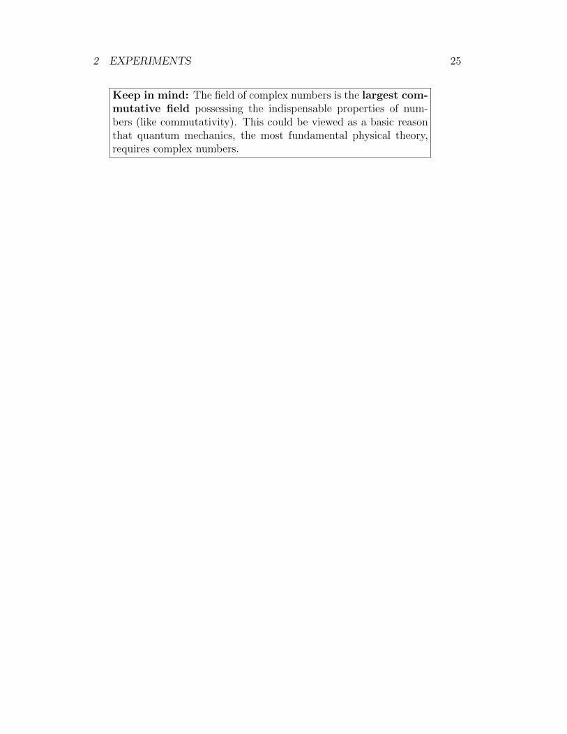
It is a well-known fact that the field of complex numbers is the largestcommutative field possessing the previous properties. This follows from atheorem of Hurwitz, see the appendix, and can be viewed as a basic reasonthat quantum mechanics, the most fundamental physical theory, uses complexnumbers and not any other systems of numbers. Another point of view is thatother number systems, like quaternions or octonions, are unlikely to appearas elementary numbers in physics, since they can be represented as matricescomposed of complex entries.

2 EXPERIMENTS 25

Keep in mind: The field of complex numbers is the largest com-mutative field possessing the indispensable properties of num-bers (like commutativity). This could be viewed as a basic reasonthat quantum mechanics, the most fundamental physical theory,requires complex numbers.

2 EXPERIMENTS 26

'

&

$

%MagneticField B

ElectricField E x

y

z

Figure 8: Propagation of an electromagnetic plane wave in direction z withhorizontal x-axis and vertical y-axis.

2.3 Polarization of Light

The classical model of light is derived from Maxwell’s equations as transverseelectromagnetic waves. Mathematically, Maxwell’s linear equations of elec-tromagnetism imply plane wave solutions

E(r, t) = E0ei(kT r−ωt), B(r, t) = 1

c(k ×E), (10)

where r = (x, y, z)T is the position vector, k = (kx, ky, kz)T is the wave vec-tor specifying the direction of propagation, ω is the angular frequency, andE,E0,B ∈ C3. The electric field E is perpendicular to the magnetic field B,and both are perpendicular to the propagation direction k. Maxwell’s equa-tions are linear per excellence and allow the superposition of solutions.

What does matter in our polarization experiments is only the classical ideathat light is an electromagnetic wave, where the electric field E and the mag-netic field B are both oscillating orthogonally in a plane which is perpendicularto the direction of motion, see Figure 8. We are free to choose the coordinatesof the direction of propagation as the z-axis together with the orthogonal xy-plane. We will choose the x-direction to be horizontal and the y-direction tobe vertical.

By convention the notion “polarization” always refers to the polarization ofthe electric field. Light has linear polarization if the electric field E oscillatesin one direction in the xy-plane. This plane can be stretched by any twoorthogonal directions, usually called the horizontal x-axis and the vertical y-axis. Linearly polarized light can be viewed as the sum or superposition of ahorizontal and a vertical component. In other words, light can be descibed bytwo base states, namely the horizontal polarization component and the verticalpolarization component.

If the electric field E rotates in the plane perpendicular to the direction ofmotion the light has circular polarization. In the latter case the rotation may

2 EXPERIMENTS 27

be either clockwise or counter-clockwise. This property is called chirality.Light carries momentum p = hk = 2πh/λ and energy hω expressed by

Planck’s constant h, wavelength λ, and angular frequency ω, respectively. Ex-periments demonstrate that light consists of a large number of small energypackets hω, the photons. The number of photons determines the intensity ofa light beam. These photons can be viewed naively as small arrows oscillatingin the plane orthogonal to the direction of propagation. Beside the concept ofpolarization, photons have further properties: they travel at the speed of light,have no charge, have no mass, and have spin one. These properties, which wefortunately don’t require, are derived in particle physics.

An optical element is a material machine that interacts with photons andchanges the state of polarization. For instance, polarizers, rotators, phaseshifters, or depolarizers are special optical elements. Most light sources emitunpolarized light, that is, a large number of photons, whose directions of oscil-lation are completely random. Light can be polarized when it passes throughan optical element.

An important optical element is a polarizer. This element is designed togenerate specific polarized light states, such as linearly or circularly polarizedstates. Absorption polarizers are characterized by the fact that they transmitlight which is polarized along one axis, the transmission axis. The light iscompletely absorbed along the perpendicular axis. Absorption is an interactionbetween the photon and the polarizer that increases the energy of the polarizer.For instance, a polaroid filter consists of molecular chains, the polymers, thatare aligned along an axis. The absorption takes place along this axis.

The wire grid polarizer has similar properties as the polaroid filter. Incidentlight, polarized parallel to the wires, causes the electrons to move inside thewires, see Figure 9. This results in a loss of some energy, and the remainder isreflected. Photons with polarization perpendicular to the wires do not interactwith the electrons, and can travel through the grid.

Birefringent plates, like calcit crystals, provide a different kind of opticalapparatus. They separate photons into two beams with perpendicular po-larization. More precisely, a calcite transmits light polarized parallel to theoptical axis along one path and transmits the remaining light polarized per-pendicular to the optical axis along another path, see Figure 10. Hence, unlikepolaroid filters, which absorb one of the components, calcits allow all photonsto pass through, but along two different paths corresponding to two polar-ization states. Hence the incident light intensity is equal to the sum of thetransmitted intensities. Birefringent plates are very flexibly applicable in ex-periments. They can be converted into optical elements similar to polaroidsby blocking one of its exit beams.

The polarization of a photon is an example of a two-state quantum system.In quantum information theory this is called a qubit, a quantum bit. There area lot of other two-state systems, for instance the spin of an electron. The spinof an electron can roughly be viewed as a small arrow as well, and a Stern-Gerlach device is comparable with a birefringent plate. Not surprisingly, themathematical models of spin and polarization are the same. But for the pur-pose of demonstration during the lectures, light is much more appropriate. In

2 EXPERIMENTS 28

'

&

$

%Figure 9: Unpolarized light interacting with a wire grid polarizer. The trans-mitted photons are polarized orthogonal to the wires.

'

&

$

%

Dy

Dx

vertically polarized

horizontally polarized

Figure 10: The birefringent plate splits incident light with respect to theiroptical axis into vertically polarized light and horizontally polarized light. Ifonly one photon is in the experiment, either detector Dx or Dy clicks.

2 EXPERIMENTS 29

Figure 11: My experimental set-up costs about 90 Euros.

particular, because optical elements such as polaroid filters and calcite crystalsare not expensive, see Figure 11.

In a similar manner the hydrogen molecule H+

2 can be described as a two-state quantum system. It consists of two protons and one electron, and theCoulomb force implies that the electron can be close to the first proton orclose to the second proton. From the mathematical point of view, all two-state systems are described within a two-dimensional Hilbert space.

Long before the term qubit was introduced, von Weizsacker31 describedqubits as the smallest building blocks of physics. He denoted these blocksby the German word “ur”. He proposed an ur theory, which is a quantumtheory of binary alternatives, that can also be viewed as a theory of the realthree-dimensional space.

The qubit is a fundamental building block, the basic unit in quantum in-formation theory. Perhaps any system, small or large, can be described bycombining these blocks via the so-called tensor product, which we considerlater. On a quantum computer, a qubit plays the same role as a bit on aclassical computer.

31von Weizsacker [1988]

2 EXPERIMENTS 30

2.4 The Law of Malus

The interaction of photons with optical elements can change the polarizationand the intensity of a beam of light, depending on the arrangement of theelements.

Let us start with a simple experiment using a polaroid filter. If we send abeam of unpolarized light through this polarizer, we observe that one half ofthe intensity of the beam is absorbed by the polarizer, and the second half istransmitted. Then we place another polarizer behind the first one, we rotatethe second one and observe that the intensity after the second filter varies. Werotate until the intensity of the light beam is maximized. It can be seen thatfor an ideal polarizer in this position the intensity after the first polarizingfilter is almost the same as the intensity after the second one. Thus bothfilters have the same transmission axis. In reality, however, there is no idealpolarizer and certain disturbances imply a slightly smaller intensity after thesecond polarizer. In the following we assume always ideal experiments.

If we rotate the transmission axis of the second filter through an angle αin small steps carefully, the light intensity decreases until the light vanishescompletely at the angle of rotation α = π/2, see Figure 12 and Figure 13.Hence, the intensity is zero if we send a beam of light through two filters withorthogonal transmission axes. A classical visualization could be to think of apolarizer in terms of a garden fence with crossbars parallel to the transmissionaxis.

Finally, we put a third filter between both polarizers. Since polarizersin general absorb light and decrease the intensity, we would expect that asbefore no light can be seen. But surprisingly and contrary to the previousvisualization of a garden fence, this is not the case, see Figure 14. Whichmathematical model is able to describe these observed unexpected intensities?

The experimental observations with different angles suggest a law that wasalready given in 1810 by Malus. The law of Malus states that the intensity I1

of a beam of polarized light that has passed both filters is given by

I1 = I0 cos2α, (11)

where I0 is the intensity after the first polarizer, and α is the angle betweenthe transmission axes of both polarizers, see Figure 12. Consequently, theintensity

J1 = I0 sin2α, (12)

is absorbed.Obviously, this law describes exactly the two experiments in Figure 12 and

13. For the third experiment in Figure 14 with three polarizers, we apply thislaw twice in succession and obtain

I2 = I1 cos2(α − β) = (I0 cos2α) cos2(α − β). (13)

For α = π/4 and β = π/2, as displayed in Figure 14, we obtain I2 = 1/4I0, whichis consistent with the experimental results. Our garden fence imagination iswrong, but the law of Malus provides a correct description.

2 EXPERIMENTS 31

'

&

$

%

unpolarized light

first polarizer

second polarizer

I0

I1

x

y

z

Figure 12: The law of Malus states that the intensity I1 of light that haspassed both polarizers is equal to I1 = I0 cos2α, where I0 is the intensity afterthe first polarizer. If only one photon is in the experiment, then cos2α is theprobability that a photon passes the second polarizer, provided it has passedthe first polarizer.

'

&

$

%

unpolarized light

first polarizer

second polarizer

I0

I1

x

y

z

2

Figure 13: For angle α = π2 between both transmission axes the intensity after

the second polarizer is zero.

2 EXPERIMENTS 32

'

&

$

%

unpolarized light

first polarizer

third polarizer

I0

I1

x

y

z

2

=4

=

second polarizer

I2 = ¼ I0

Figure 14: If we put a third polarizer between both polarizers with transmissionaxis rotated about α = π

4 , then the intensity is I2 = 14I0.

The average value cos2α for varying angle α is 1/2. Therefore, the trans-mission coefficient of a beam of unpolarized light, containing a uniform mixtureof linear polarizations at all possible angles, should be 1/2. Almost all naturalsources of light emit unpolarized light.

In actual experiments the light intensity can be reduced such that only onesingle photon is in the experiment. Then the intensity of a beam of light isgiven by the number of photons yielding the following interpretation:

• For a photon the squared quantity cos2α can only be interpreted as aprobability, namely the probability that it will be transmitted. Theprobability that it will be absorbed is sin2α.

Notice that cosα has positive and negative values. Hence, the law of Malusrequires squared magnitudes.

The law of Malus formulated in 1810 for intensities becomes Born’s rulefor single photons. This rule was formulated in 1926, and was awarded 1954by the Nobel Prize in Physics. By the way, the rules of classical probabilitywere formulated much later by Kolmogorov in 1933.

In terms of classical probability theory equation (13) has the followinginterpretation: the probability that a photon passes all three filters, when ithas passed the first filter, is cos2α ⋅ cos2(α − β) which is the classical productrule for independent events. This is in agreement with the experiments, atleast for ideal polarizers.

Keep in mind: Simple experiments with light, already performedby Malus in 1810, demonstrate: when accepting that light is builtup of photons, the interaction of photons with optical elements isa stochastic process, and the probabilities of the random outcomesare squared magnitudes of numbers.

2 EXPERIMENTS 33

'

&

$

%Figure 15: An almost lossless rotation from vertical polarization to horizontalpolarization with polaroid filters.

The law of Malus has the fascinating property that it is perfectly symmetric.What is the symmetry of a law? Symmetry of geometrical objects is usualdefined as a property of an object that does not change if something changes.Spheres do not change if they are rotated by an arbitrary angle. A squareremains invariant when rotated by a right angle. Crystals, like snowflakes,have a beautiful symmetry. For physical laws the symmetry is rather similar.Equations are written down using certain letters. In our case of polarization,we use x and y to describe the horizontal and vertical direction, and we useα and β to describe angles related to transmission axes. But we are freeto choose any other orthogonal directions using letters x′, y′ and angles α′,β′. An equation describing a physical law is symmetric if it looks the same,independent of whether it is described by the primed or unprimed coordinates.Obviously, the law of Malus is the same in each coordinate system since theidentity

cos2(β − α) = cos2(β′ − α′) (14)

yields exactly the same probability. The law requires only the difference be-tween two angles, rather than some absolute angles. All fundamental lawsof physics are symmetric in this sense; they look the same in every referenceframe.

Since in the law of Malus only the difference of the angles between bothtransmission axes is relevant, it follows that the polarization of the photonbefore both polarizers in series doesn’t matter. The photon has completelyforgotten the history. Moreover, we have seen that when placing a polarizerappropriately between two others, as displayed in Figure 14, the intensity

2 EXPERIMENTS 34

increases. We can easily generalize this experiment. Assume, we put a largenumber of polaroids, say N , with transmission axes differing only by a smallangle, between two polaroids with perpendicular transmission axes, see Figure15. Then the law of Malus (13) implies that the probability for a vertically

polarized photon to pass all polaroids is (cos(π/2N ))2N . Then the photon ishorizontally polarized. For N = 18 we roughly get the probability 0.9337.Thus this experimental set-up causes an almost lossless rotation from verticalto horizontal polarization. Of course, an analogous set-up for an almost losslessrotation from horizontal to vertical polarization is possible as well.

2 EXPERIMENTS 35

'

&

$

%

Dy

Dx

100%

0%

Figure 16: For two birefringent plates, where the horizontal light after the firstplate is blocked, only the vertical detector Dy clicks. If we block the verticallight after the first plate, then only the horizontal detector Dx clicks.

2.5 Birefringent Plates

In the following we discuss some experiments with birefringent plates.At first we introduce a useful notation which allows us to describe experi-

ments in a neat form. It is called Dirac’s bracket notation. For instance, if aphoton, has passed a polarizer with transmission axis α, it is linearly polarizedat this angle, and we write ∣α⟩ for this state. Moreover, we assign to any tran-sition from one initial state ∣α⟩ to another state ∣β⟩ a complex number (arrow)

⟨β∣α⟩ ∈ C. (15)

This complex number, written as a bracket, is called a probability amplitude.Notice that the initial state ∣α⟩ is on the right hand side of the bracket, andthe final state ∣β⟩ is on the left hand side. This chronological order is usual inquantum physics.

The probability of this transition is given by Born’s rule

Prob(⟨β∣α⟩) = ∣⟨β∣α⟩∣2. (16)

as the squared magnitude of the amplitude, and is called the transition prob-ability. This is a generalization of the law of Malus who used only real ampli-tudes that are sufficient for linear polarization.

Now we discuss the experiments displayed in Figures 16, 17, 18, and 19.The experiments in Figures 16, 17 and 18 follow immediately from the law ofMalus. Details are left as an exercise. The experiment displayed in Figure19 is the most difficult example to explain. In this experimental set-up, bothbirefringent plates recombine both beams after the first polarizer. Therefore,the law of Malus or Born’s rule yields the transition probability

∣⟨β∣α⟩∣2 = cos2(β − α) (17)

after the second polarizer.The usual way to obtain this result is to calculate the probabilities for a

photon travelling through the apparatus by using the classical addition rule for

2 EXPERIMENTS 36

'

&

$

%

Dyy 25%Dyx

Dxy

Dxx

25%25%25%

± π 4

π 4

Figure 17: A beam of photons is polarized in state ∣ + π4 ⟩ by an appropriately

oriented polaroid filter. The photons pass horizontally or vertically the firstbirefringent plate, then they pass through the second plate with an opticalaxis rotated at an angle +π4 or −π4 . Finally they are detected. It follows thatthe photons have forgotten their original polarization state ∣ + π

4 ⟩.

'

&

$

%

Dy

Dx

50%50%

± π 4

Figure 18: In this experimental set-up the horizontally polarized photons areblocked after the first two birefringent plates. Finally, after the third plate theirpolarization is measured. Obviously they have lost their original polarization.

2 EXPERIMENTS 37

'

&

$

%

y y

Figure 19: The first polarizer generates photons polarized at an angle α. Thefirst birefringent plate splits into two beams of horizontally x-polarized andvertically y-polarized photons. These are recombined in a second birefringentplate which has an optical axis opposite to the first plate. According to thelaw of Malus the transition probability after the second polaroid is cos2(β−α).

mutually exclusive events and the multiplication rule for independent events. Ifwe do this, we see that after the first polarizer the photon is linearly polarized atan angle α. The first calcite generates a horizontally and a vertically polarizedbeam. The equations (11) and (12) imply that the photon is in one of thebeams with probabilities

cos2α or sin2α, (18)

respectively. If the photon is vertically polarized it passes the second bire-fringent plate with probability one, and the second polarizer with transitionprobability

∣⟨β∣0⟩∣2 = cos2 β, (19)

since the optical axis of the plate and the transmission axis of the secondpolaroid differ by an angle β. Similarly, we obtain the transition probability

∣⟨β ∣π2⟩∣

2

= sin2 β, (20)

if the photon is vertically polarized. Due to the split into a horizontally and avertically polarized beam, we have two mutually exclusive paths

∣α⟩→ ∣0⟩→ ∣β⟩ and ∣α⟩→ ∣π2⟩→ ∣β⟩. (21)

The sub-paths are independent. Hence, the probabilities of the sub-paths aremultiplied, yielding for each path the probability

cos2α ⋅ cos2 β and sin2α ⋅ sin2 β, (22)

respectively. With the addition rule we get the transition probability after thesecond polarizer

Prob(⟨β,α⟩) = cos2α cos2 β + sin2α sin2 β, (23)

2 EXPERIMENTS 38

which obviously is in disagreement with cos2(β−α) and also with experimentalstatistics. Classical probability theory does not work.

In order to obtain the correct result, we change the rules for calculatingthe probabilities by using amplitudes. Instead of adding the probabilities formutually exclusive events, we add the non-squared amplitudes for these eventsand multiply the probabilities for independent events. We apply both rules tothe amplitudes and then we square the magnitude of the final result. Theseare Feynman’s rules for quantum phenomena. Then we get

⟨β∣α⟩ = ⟨β∣0⟩⟨0∣α⟩ + ⟨β ∣π2⟩ ⟨ π

2∣α⟩

= cosβ cosα + sinβ sinα

= cos(β − α),

(24)

yielding the desired result

∣⟨β∣α⟩∣2 = cos2(β − α). (25)

This prediction is in agreement with experiments. In particular, the probabilityamplitudes satisfy the superposition principle: the amplitudes for both pathsare added.

Notice that all previous experiments did only require positive and negativenumbers in terms of sine and cosine, but not complex numbers. It turnsout, however, that complex numbers are necessary when we discuss circularlypolarized light.

2 EXPERIMENTS 39

'

&

$

%

+2

+1

0

-1

-2

source wall withslits a,b screen detectors

s

b

a d1|a

d2

d1

d0

d-1

d-2

Figure 20: The double-slit experiment described for a discrete spacetime. Theparticle leaves source s, passes one of the two slits a or b, and is finally detectedin d1.

2.6 The Double-Slit Experiment

The double-slit experiment with its diffraction pattern has been called “Themost beautiful experiment in physics32”. The used experimental set-ups de-pend on the type of particles acting in the two-slit experiment. It can be donewith photons or electrons, and becomes more difficult for increasing size of theparticles. Until now, the largest molecules showing interference, are combinedof 810 atoms.

We consider a source of particles, say photons, electrons or fullerene. Forthe sake of convenience, we assume a discrete space consisting of points

(m, t), m = −2,−1,0,1,2, t = t0, t1, t2, (26)

where m denotes five spatial points at three times t, as displayed in Figure20. It makes no difference for the mathematical treatment, if we choose amuch finer grid, for instance with 10100 points, leading to an approximation ofspacetime much more finer than the accuracy of any measurements.

At time t0 a particle leaves the source s, arrives at time t1 at the wall withtwo slits a and b, and is detected at time t2 in exactly one of the detectors dm.We ask for the probability that the particle is detected at point m.

If we use classical probability theory, then the particle arrives at m eitherthrough slit a or through slit b. These are two mutually exclusive events that

32Crease [2002]

2 EXPERIMENTS 40

add up to the total probability

Prob{⟨dm∣s⟩} = Prob{⟨dm∣a⟩}Prob{⟨a∣s⟩}

+Prob{⟨dm∣b⟩}Prob{⟨b∣s⟩}.(27)

If the probability of passing slit a is the same as passing slit b, thus is 1/2, weobtain

Prob(⟨dm∣s⟩) = 1

2Prob(⟨dm∣a⟩) + 1

2Prob(⟨dm∣b⟩). (28)

Since probabilities are always non-negative, their addition does not lead to anycancellation or destructive interference. This contradicts experimental results,since interference is observed if both slits are open, see Figures2133 and 22 .

Now we try to explain this experiment by using Feynman’s quantum prob-ability rules: the amplitudes are multiplied for independent events, are addedfor mutually exclusive events, and are squared, finally. Firstly, we assume thatslit b is closed. The probability amplitudes ⟨a∣s⟩ = 1, ⟨b∣s⟩ = 0, ⟨dm∣a⟩ = ψm,and ⟨dm∣b⟩ = ϕm combine to

Prob{⟨dm∣s⟩} = ∣⟨dm∣a⟩⟨a∣s⟩ + ⟨dm∣b⟩⟨b∣s⟩∣2

= ∣⟨dm∣a⟩ ⋅ 1 + ⟨dm∣b⟩ ⋅ 0∣2

= ∣ψm∣2.

(29)

Thus we obtain a classical probability without any interference. Secondly, weassume that slit a is closed. Then ⟨a∣s⟩ = 0, ⟨b∣s⟩ = 1, and as above we get

Prob{⟨dm∣s⟩} = ∣ϕm∣2. (30)

Finally, we assume that both slits are open. The probability calculated byFeynman’s rules with ⟨a∣s⟩ = ⟨b∣s⟩ = 1

√

2is

Prob{⟨dm∣s⟩} = ∣⟨dm∣a⟩⟨a∣s⟩ + ⟨dm∣b⟩⟨b∣s⟩∣2

= ∣ 1√

2ψm + 1

√

2ϕm∣2

= 12(ψm + ϕm)∗(ψm + ϕm)

= 12(ψ∗mψm + ψ∗mϕm + ϕ∗mψm + ϕ∗mϕm)

= 12 (∣ψm∣2 + ∣ϕm∣2) + 1

2(ψ∗mϕm + ϕ∗mψm).

(31)

Comparing with (28), (29), and (30), it follows that the first term in thissum corresponds to the classical probability, and the second term describesinterference.

This can easily be seen as follows. For points m with ψm = ϕm we obtainfrom (31)

Prob{⟨dm∣s⟩} = 2∣ψm∣2. (32)

33Belzasar [2012]

2 EXPERIMENTS 41

'

&

$

%Figure 21: Results of a double-slit-experiment performed by Dr. Tonomurashowing interference. The numbers of electrons are 11 (a), 200 (b), 6000 (c),40000 (d), and 140000 (e). The electrons were shot one by one through thedouble-slit so that they could not interfere with each other.

2 EXPERIMENTS 42

'

&

$

%

s

a

b

detectorspath a path b sumwall with

two slits

particlesource

Figure 22: Schematic illustration of the double-slit experiment. The arrowsrepresent the complex amplitudes for each path and their sum. Squaring themagnitude of the sum determines the corresponding probability. This leads todestructive and constructive interference, as displayed on the wall of detectors.

This doubles the classical probability, where only one slit is open. Hence,we have constructive interference. If ψm = −ϕm, the probability to find theparticle at point m is

Prob{⟨dm∣s⟩} = 0, (33)

yielding destructive interference. For other combinations we obtain probabili-ties that are between both extreme cases, as displayed in Figure 22.

Until now we don’t have the correct values for all amplitudes, such as ψmand ϕm. In order to calculate the amplitudes for going from one position toanother we need the classical physical action of this process, usually denotedby S. In classical mechanics the action is a well-known concept. Roughlyspoken, the action is the Lagrangian, that is the difference between the kineticenergy and the potential energy, integrated over a path where a particle maymove. For a free particle (no forces act on it) the Lagrangian is just the kineticenergy. Classically, the path taken by the particle actually is a stationary pointof the action S. This rule is called Hamilton’s principle of least action.

In non-relativistic classical mechanics a free particle is an object where noforces act on it. It has only kinetic energy p2/2m, and the action to go fromposition r1 to position r2 is the integral over time, taken along the path between

2 EXPERIMENTS 43

both positions. In first order the action is S = p(r2−r1). The amplitude ⟨r2∣r1⟩of a path between positions r1 and r2 is proportional to the complex number

⟨r2∣r1⟩ = eiS/h = eip(r2−r1)/h, (34)

where h is Planck’s constant.In the relativistic case, the only difference is that the momentum p is related

to the well-known energy-momentum relation

E2 = (pc)2 + (m0c2)2 (35)

with particles’s rest mass m0, the speed of light c, and assuming the flatMinkowsi spacetime in special relativity.

Equation (34) can be viewed as a complex plane wave with wave numberequal to the momentum divided by Planck’s constant. More precisely, theparticle is at some time t at some place r such that actually we have a time-dependent amplitude ⟨r2, t2∣r1, t1⟩. In the nonrelativistic case, when looking atthe limit t2 → t1, the amplitude is a function of time and it can be shown thatit satisfies the well-known Schrodinger’s wave equation.

Finally, we want to discuss the case that in the double-slit experimentwe can get information about which slit the particle passes through. Thisinformation can be given by two detectors da and db that click when a particlepasses slit a or b, respectively. Of course, detectors may fail and informationmight be wrong.

Looking at the experiment displayed in Figure 23, we have the event that aparticle is detected at point m and the detector da or db clicks. We consider inthe following this type of events, although we could easily incorporate eventswhere a particle is detected in m, but neither one of da or db clicks.

The amplitude that a particle goes from source s via slit a to point m anddetector da clicks is

⟨m∣da⟩⟨da∣a⟩⟨a∣s⟩. (36)

But it may also happen that a particle arrives at m via slit b and detector daclicks. This possibility has the amplitude

⟨m∣da⟩⟨da∣b⟩⟨b∣s⟩, (37)

and should happen rarely, provided the detectors work well. Other mutuallyexclusive possibilities do not occur, as can be seen from Figure 23. Accordingto our addition rule we have to add both amplitudes

⟨(m,da)∣s⟩ = ⟨m∣da⟩⟨da∣a⟩⟨a∣s⟩ + ⟨m∣da⟩⟨da∣b⟩⟨b∣s⟩ (38)

for the outcome that a particle arrives at m from source s and detector daclicks. The corresponding probability is

Prob{⟨(m,da)∣s⟩} = ∣⟨(m,da)∣s⟩∣2. (39)

If the detectors are perfect, then the probabilities

Prob{⟨da∣a⟩} = 1 and Prob{⟨da∣b⟩} = 0, (40)

2 EXPERIMENTS 44

'

&

$

%source wall with

slits a,b screen detectors

s

b

(2, da)

a

(2, db)

(1, da)(1, db)

(0, da)(0, db)

(-1, da)(-1, db)

(-2, da)(-2, db)

slit-detectors

da

db

Figure 23: The double-slit experiment with slit-detectors. There are two pathsfor the event that a particle arrives at point 2 and detector da clicks. For theother points there are two paths as well.

yielding ⟨da∣a⟩ = 1 and ⟨da∣b⟩ = 0. Assuming ⟨a∣s⟩ = 1√2

gives

Prob{⟨(m,da)∣s⟩} = ∣⟨m∣a⟩⟨a∣s⟩∣2 = 1

2∣ψm∣2, (41)

which is the classical probability as in (28).With the same arguments as before, we obtain the amplitude

⟨(m,db)∣s⟩ = ⟨m∣db⟩⟨db∣a⟩⟨a∣s⟩ + ⟨m∣db⟩⟨db∣b⟩⟨b∣s⟩ (42)

for the event that a particle arrives at point m from source s and detector dbclicks. For an ideal detector ⟨db∣a⟩ = 0, and assuming ⟨b∣s⟩ = 1

√

2we obtain the

classical probability

Prob{⟨(m,db)∣s⟩} = ∣⟨m∣b⟩⟨b∣s⟩∣2 = 1

2∣ϕm∣2. (43)

This seemingly surprising result can be explained easily. The reason is that theoutcomes have changed from spacetime points m to spacetime points (m,da)and (m,db) with detectors. A change of the outcome implies a change of theprobabilities. That’s all, nothing strange happened.

On the other hand, if both detectors don’t work, say all amplitudes ⟨da∣a⟩,⟨da∣b⟩, ⟨db∣a⟩, and ⟨db∣b⟩ are equal to some value α, then the total amplitude

2 EXPERIMENTS 45

becomes

⟨m∣s⟩ = ⟨(m,da)∣s⟩ + ⟨(m,db)∣s⟩= α ⋅ ( 1

√

2ψm + 1

√

2ϕm). (44)

Comparing with (31), it follows that this is the probability if both slits areopen, except for the pre-factor. Thus we have interference as in the casewithout any detectors.

2 EXPERIMENTS 46

'

&

$

%

s

wall with slitsi=1, …, N

source

wall with slitsj=1, …, M

a path

i

j

screen of detectors

x

Figure 24: Two walls with multiple slits i = 1, . . . ,N and j = 1, . . . ,M .

2.7 Diffraction at Multiple Slits

In this section we shall generalize our results for the double-slit experiment tomultiple slits. Moreover, we shall derive computable probability amplitudes.

Let us consider the more complicated interference experiment as displayedin Figure 24.

There are several paths: the particle can go from the source s through somehole i in the first wall, then through some hole j in the second wall, and finallyto a detector x at the screen, yielding the amplitude

⟨x∣j⟩⟨j∣i⟩⟨i∣s⟩. (45)

All these paths from the source to any detector describe possibilities. Theparticle could move in a future action on this path from s to x as well as onanother path from s to x. Therefore, the amplitude to arrive at a specificposition x is the sum of all related amplitudes, that is,

⟨x∣s⟩ = ∑i=1,...,Nj=1,...M

⟨x∣j⟩⟨j∣i⟩⟨i∣s⟩. (46)

Of course, this sum can easily be generalized to an arbitrary number of wallswith an arbitrary number of slits with infinitesimal distances. Then the sum(46) becomes an integral, namely the path integral.

It will turn out that the single amplitudes depend on the geometry of theexperimental set-up and the particles in the experiment. We will now derivethe concrete amplitudes in the case of photons with diffraction at one wallonly.

2 EXPERIMENTS 47

What is the idea behind calculating the concrete amplitudes? Photon’sdo not appear smoothly. Contrarily a photomultiplier clicks randomly, thusshowing their discrete nature. A photon is a massless and chargeless particletravelling with the speed of light c in form of lumps of energy. The rulefor obtaining the probability amplitude, and thus the chance of this path, isderived by computing the action Spath and forming the complex arrow e

ihSpath ,

where h = 2πh is the Planck constant.Hence, our remaining problem is to find the kinetic energy of a photon.

Photons move with the speed of light c, and thus should be described in ac-cordance with the theory of special relativity. There, particles satisfy therelativistic energy-momentum equation

E2/c2 − (px)2 − (py)2 − (pz)2 =m2c2, (47)

where the three-vector p = (px, py, pz) is the relativistic momentum

p = γmv, where γ = 1√

1 − vc

2, (48)

and

E = γmc2 (49)

is the relativistic energy. Defining the energy-momentum four vector as pµ =(E/c, px, py, pz), it follows that the relativistic energy-momentum equation statesthat the quantity on the left hand side is relativistically invariant with respectto Lorentz transformations, and is equal to the squared rest energy. Especiallythis equation shows a beautiful symmetry in the relativistic spacetime.

A closer inspection exhibits a loophole for massless particles, since for m = 0the numerators in equations (48) and (49) are zero. But if we demand thatmassless particles move at the speed of light v = c, then also the denominatorsvanish, and the relativistic energy-momentum equation is formally fulfilledwhen we set

v = c and E = ∣p∣c. (50)

Actually, these are at most formal assignments. It is not clear where the energyand the momentum of a massless particle come from. In physics, however, aphoton is defined as the energy lost by an electron when jumping from anexcited state to a state of lower energy, yielding the equation

E = eV and ∣p∣ = E/c. (51)

where eV denote electronvolts. It is well-known that the energy determinesthe color of light. Moreover, we see that the energy is independent of the path.Photons have no position.

The action is the integral, or sum if you like, along the path. It followsthat for any photon the action is equal to Etpath. The quantity tpath is just theparameter describing the required time for the photon to get from the starting

2 EXPERIMENTS 48

point of the path to the final point. Since the photon moves with constantvelocity, the required time is proportional to the length of the path, the latteran important geometrical property. This geometrical quantity defines mainlyour amplitude.

Classically, light is an electromagnetic wave. The quotient ω ∶= E/h iscalled angular frequency of light, and ν = ω/2π is the frequency of light. Fre-quency and the speed of light are combined by the equation c = λν, where λis the wavelength. Thus a high frequency, or equivalently a short wavelength,determine high energy photons.

Using the previous quantities, the action Spath, related to a given path, isthe energy multiplied by the time, that is,

Spath = h ω tpath. (52)

Dividing the action by h yields a dimensionless number, namely the probabilityamplitude for the path

⟨point x ∣ start s⟩via path = eihSpath = eiωtpath . (53)

In fact, this amplitude looks like a stopwatch that is started when thephoton leaves the source. This stopwatch rotates very rapidly correspondingto the action for this path - this is about 36 000 times per inch for red light- until the photon reaches the photomultiplier. At this moment the watch isstopped, and the hand points in a certain direction, yielding the small arrowcalled the amplitude.

Suppose we have a wall with N slits as displayed in Figure 25. Then for aphoton that passes slit xn = x0 − nd, x0 = 0, n = 0,1, . . . ,N − 1 and arrives atsome point x on the screen of detectors, the formula (53) takes the form

ψn(x) = ⟨point x ∣ start s⟩via xn = eiωteiω√

(x−nd)2+L2. (54)

There, t is the time that the photons needs to go from the source to slit xn.Of course this time depends on the related slit. We assume that n is small,and the distance from the source to the wall of slits is large compared to thedistance d between the slits. We set c = 1 such that x = ct = t. Thus time anddistance are equal. The square root in the second exponential term is exactlythe distance between the slits and the detectors. The action as an integral isadditive, and the multiplication rule for the exponential function implies theproduct of both exponential terms.

If we assume additionally that the distance d between two slits is smallcompared to the distance L from the slits to the screen of detectors, we canwrite

√(x − nd)2 +L2 ≈ L(1 + 1

2

(x − nd)2

L2) = L + x2

2L− xnd

L+ (nd)2

2L, (55)

where higher order terms of d are neglected. Therefore, for a photon passingslit xn, we get the approximate amplitude

ψn(x) = eiω(t+L+x2

2L)e−iω(

xndL−(nd)2

2L). (56)

2 EXPERIMENTS 49

'

&

$

%

ssource

N slits

x0=0

back stop with detectors

d

d

x0-2d

L

r

x

Figure 25: A wall with N slits, with distance d between two slits, and distanceL from the slits to the back stop of detectors.

Superposition over all slits yields the final amplitude

ψ(x) = Aeiω(t+L+ x2

2L)

N−1

∑n=0

e−iω(xndL−(nd)2

2L), (57)

for a photon passing any slit, which we don’t know, and arriving at detectorx. The constant A is a necessary normalization constant such that all squaredmagnitudes are classical probabilities and sum up to one. The function ψ(x)of amplitudes depends mainly on the geometry of the experimental set-up, notso much on the photon itself. The contribution of the photon is its frequencyonly, or equivalently its energy.

The slit experiments are rather mysterious and strange. At the back-stop the particles arrive as small lumps demonstrating a point-particle likebehaviour. They show a classical statistical point-like behavior whenever onlyone of the slits is open, or if we obtain information through which slit theparticle has gone. But if the slits are open, and if it is not decidable throughwhich slit the particle passes, then we obtain an interference pattern.

These results can be obtained also with the same mathematics that de-scribes sound waves or water waves, except that we use complex numbers inquantum mechanics, not real numbers. If waves meet the wall of slits, then ateach slit diffraction generates a radial wave traveling radially away from theslit, according to Huygens’ principle, well-known in wave theory. These radialwaves superpose, and summing them up returns an intensity distribution of awave that shows the same interference as ψ. This is one reason for the well-known wave-particle duality. Nevertheless, the particles arrive as lumps at the

2 EXPERIMENTS 50

backstop in contrast to real waves, and we should have in mind what Feynmanwrites:

Keep in mind:

However, it must be emphasized that the wave func-tion [of amplitudes] that satisfies the equation is not likea real wave in space; one cannot picture any kind of re-ality to this wave as was done to a sound wave.

Feynman34

In other words, the wave function of amplitudes may mathematical looklike a real wave, but actually it is not a wave. It implies merely a probabilitydistribution.

Similar results can be obtained when performing diffraction experimentswith particles that have mass. For free electrons and other free massive par-ticles traveling with low speeds we can use the non-relativistic kinetic energy12mv

2 leading to the complex arrow eihSpath that rotates with

rate of rotation = mv2

2hturns per sec. (58)

When teaching quantum physics electron diffraction at multiple slits is usuallydiscussed as thought experiments. An exception is Jonsson’s article35 thatdescribed already in 1961 a realization in the laboratory with electrons up tofive slits. Besides the educational value of this precise experimental description,with this set-up neither single particle diffraction nor close individual slits canbe observed. In 2013 Bach et al.36 presented a full realization of this famousthought experiment.

If the particles are not free but forces act on it, then the Lagrangian isthe difference between the kinetic and the potential energy. The kinetic en-ergy depends only on the velocity, and the potential energy comes from thegravitational force acting on space points. Let us throw a ball in the air, thenHamilton’s principle of least action says that the ball follows a parabola, whichis the path of least action.

In classical mechanics a force is interpreted as something that pulls orpushes, even over long distances. In the theory of general relativity a force isdetermined through the curvature of spacetime. From our stochastic point ofview, the difference between the action along a path with and without potentialenergy is the change of the phase angle of our amplitudes. In other words, thedirection of the complex arrows is changed.

34Feynman Lectures [1963, Vol. 3, pp. 3–4]35Jonsson [1974]36Bach et al. [2013]

2 EXPERIMENTS 51

Keep in mind:

A modern stochastic point of view of what forcesare, is as follows: a force changes the action and thusphases, that is, the directions of probability amplitudes.

2 EXPERIMENTS 52

1 2 3 4 5 6 7 8 9 10 11 12 13

WallS P

Figure 26: The classical view of the ray model: the mirror reflects light suchthat the angle of incidence is equal to the angle of reflection.

1 2 3 4 5 6 7 8 9 10 11 12 13

WallS P

Figure 27: Feynman’s view says that light has an amplitude equal in magnitudefor each possible path from the source to the photomultiplier. In particular, itcan be reflected from every part of the mirror, that is, from the middle as wellas from the other parts.

2.8 Light Reflection

In this section we investigate Feynman’s quantum probability predictions forthe seemingly simple problem of how light is reflected by a mirror, see Figure26. The experimental set-up is as follows: at a source, light of one color isemitted, and at another point there is a photomultiplier for detecting light.We use a very low light intensity such that some time passes between the clicksof the photomultiplier. In other words, only one photon is in the experimentat any time. To prevent a photon from going straight across to the detectorwithout being reflected, a wall is placed in the middle.

The well-known ray model of light in optics says that the mirror reflectslight in a way such that the angle of incidence is equal to the angle of reflection.Moreover, the length of the mirror as well as the right and the left end of themirror have no influence on the light that reaches the detector. This modeldescribes light in terms of rays and holds true in many practical situations.

In Feynman’s formulation of quantum probability the photon has also thepossibility to take any other path. Only paths through the wall are forbidden.Each possible path is furnished with a reasonable amplitude as displayed inFigures 27 and 28. Remember that we have seen that the action of the photonalong any path corresponds to the length of this path, not to the path itselflike the action of mass particles.

This is the way how the well-known wave-particle duality is resolved inFeynman’s formulation: the photon has no complementary partner such as a

2 EXPERIMENTS 53

1

23

4 56

7

8

9 10

1112

13

Figure 28: The amplitudes for all possible paths are added together. Themajor contribution to the final arrow’s length is made by the paths of minimalaction, that corresponds to the paths of minimal length.

the wave. Instead paths are equipped with arrows, the probability amplitudes,satisfying the general rule: For each path from the source to the photomulti-plier draw an appropriate arrow, add all arrows with parallelogram addition.This is, the quantum rule of superposition. Then square the magnitude of theresulting arrow. This returns the probability of being detected by the photo-multiplier. These are the same stochastic rules as stated in the sections before.It makes any wave pictures superfluous in Feynman’s formalism.

The probability amplitude for the outcome that a photon starts at sources and is detected by the photomultiplier at point p is

⟨p∣s⟩ = ∑all paths

eihSpath . (59)

At a first glance, we guess that a photon should simultaneously take all possiblepaths from s to p, a strange visualization, that is mentioned in many textbooks.The action Spath for photons, however, depends only on the length of thepath or equivalently on the time tpath. This is a geometrical property of theexperimental set-up. Thus, the amplitudes don’t require that the photonsmust actually interact with all paths. They just describe possibilities37.

The small arrows in this sum are displayed in Figures38 27 and 28, where wehave divided the mirror into little squares, with one path for each square. Whenwe add all contributions for the paths, then, as seen in Figure 28, the final arrowlength evolves mainly from arrows of the middle part of the mirror, whereasthe contributions from the left and right part almost cancel out each other.All paths in the middle part have almost the shortest length, corresponding tothe well-known classical principle of least action.

More precisely, for all paths from the source to the photomultiplier, theaction Spath is very large compared to Planck’s constant. Therefore, for nearbypaths the amplitudes differ very much, since a relatively small change of theaction is large compared to h thus yielding a completely different phase. Thisimplies cancellation of the arrows in the sum.

There is only one exception, namely the paths that are infinitesimally closeto the path of least action, also called the extremal paths. In this case the first

37The usual interpretation of this experiment can be found in the nice talk of Girvin inthe KITP Public Lectures, see online kitp.edu/online/plecture/girvin.

38The figures in this section are modifications of related ones in the book Feynman [1985]

2 EXPERIMENTS 54

1 2 3

Figure 29: Considering only the piece of the left part of the mirror, the detectordoes not click, since the amplitudes add up to approximately zero.

variation of the action is zero. This implies that nearby paths have almost equalaction, and thus have equal amplitudes in the first approximation. Exactlythese paths are the important ones and contribute coherently. This occurs inthe region where the arrows almost point in the same direction.

In other words, all paths distant from the classical path of least actioninterfere destructively. On the other hand, the paths in the neighbou rhoodof the classical path interfere constructively. This is the reason why we ob-serve mainly classical events, such as light travels in a straight line where thetime is shortest. This fact was already discovered in 1650 by Fermat and iscalled Fermat’s principle of least time. This principle is the success of the raymodel in optics. Only the middle part of the mirror seems to be responsiblefor reflections. It is really surprising, however, that the stop watch rotatesten thousands of times until the photon reaches the photomultiplier, but theamplitude for this event is the final hand direction of the watch.

But that is not the whole story. The basic question is: how does thephoton find the path of extremal action? Does the photon smell out all possiblepaths in order to find the right one. Or is this approach only a mathematicaldescription far away from any reality? If this formalism has any reality, weshould be able to show in an experiment that a photon sometimes chooses alsoother paths, shouldn’t it?

It is simple to answer these questions using the following experiment. Wecut off a large part of the mirror such that only three segments on the left sideare left over, see Figure 29. Moreover, the amplitudes are displayed in greaterdetail. If we add all arrows, we see that they cancel out, and the probabilityto be detected in the photomultiplier is almost zero.

But if Feynman’s theory is true then photons should be detected when wereduce the left part of the mirror in a manner such that no cancellation can oc-cur, see Figure 30. Then the majority of arrows points to the right, and in totalwe obtain an amplitude that predicts a strong reflection. In fact, in agreementwith our theory, the photomultiplier clicks sometimes. This sounds crazy:in theory as well as in practice you cut off the important middleof the mirror, from the remaining part you scrape away appropri-

2 EXPERIMENTS 55

1 2 3

Figure 30: A striped mirror reflects a substantial amount of light, and is calleda diffraction grating.

S Blue

Red

Figure 31: The angle of reflection depends on the color (wavelength) of light.

ate pieces, and then you observe reflection. Once more, the photonseems to walk on each possible path with a stopwatch.

Some further remarks should be given. The size of the experiment, theplacements of source, photomultiplier and cut-out’s of the mirror, and hencethe direction of the arrows depend also on the colour of the light, hence onits energy or equivalently its frequency. This follows from the definition of theaction that depends on the frequency or equivalently on the wavelength.

For other particles such as electrons or atoms Feynman’s formalism worksjust as well. There the action is replaced by the integral over the differencebetween kinetic and potential energy along the considered path.

Keep in mind: Feynman’s theory, a pure particle formalism with-out any waves, shows the close relationship between the determin-istic classical mechanics, described by Hamilton’s principle of leastaction, and quantum mechanics as a stochastic process with com-plex probability amplitudes. Both theories have in common thatthe particle prefers the path for which the action does not vary inthe first approximation. The considered paths are not assumed tobe smooth, they can exhibit a zig-zag curve as in Wiener processes.

2 EXPERIMENTS 56

'

&

$

%

source s0

source s1

|0

|1'

|0''

|1''

|0'

|1 mirror

m1

m2

b1

b2

d1

d2

Figure 32: A Mach-Zehnder interferrometer.

2.9 Interferometer

The Mach-Zehnder interferometer is a device used, for instance, in electro-optic modulators, integrated circuits, electronic devices, and also in quantuminformation theory. It serves as a nice apparatus demonstrating the funda-mental rules of quantum mechanics. The set-up, see Figure 32, is as follows.A beam of particles, say photons, is split by a beam splitter b1, for instance ahalf-silvered mirror. The two resulting beams are reflected by two mirrors n1

and m2. Then they pass through a second beam splitter b2 and finally entertwo detectors d1 and d1. This experiment can be viewed as a special versionof the double-slit experiment, where the photon or the electron can traverseon exactly two paths.

If a single photon enters the interferometer, either from path ∣0⟩ or path∣1⟩, it interacts with the first beam splitter. We assign the passage througha beam splitter by the amplitude 1

√

2. Since the squared amplitude is 1

2 , it is

a 50/50 percent beam splitter. The beam-splitter transforms the path of thephoton into a two-state system, namely moving horizontally or vertically. Thisis also called a path qubit.

The number i = eiπ/2 is the probability amplitude when the photon is re-flected, and the path is rotated by a right angle. Since ∣i∣2 = 1, the probabilitythat a photon is reflected is one, as expected.

Now, let us calculate the amplitude that the photon, starting at source s0,

2 EXPERIMENTS 57

is detected in d1. The first path is from below yielding

⟨d1∣1′′⟩⟨1′′∣0′⟩⟨0′∣0⟩ =i√2⋅ i ⋅ 1√

2= −1

2, (60)

and from above we get

⟨d1∣0′′⟩⟨0′′∣1′⟩⟨1′∣0⟩ =1√2⋅ i ⋅ i√

2= −1

2.

Both paths represent two possibilities. There are no other paths arriving atdetector d1. Thus, adding both amplitudes we obtain the total probabilityamplitude

⟨d1∣0⟩ = −1

2− 1

2= −1. (61)

Hence, with probability (−1)2 = 1 the photon will be detected in d1.The amplitude, for the photon to be detected in d2, is the sum of

⟨d2∣0′′⟩⟨0′′∣1′⟩⟨1′∣0⟩ =i√2⋅ i ⋅ i√

2= − i

2, (62)

and

⟨d2∣1′′⟩⟨1′′∣0′⟩⟨0′∣0⟩ =1√2⋅ i ⋅ 1√

2= i

2. (63)

Hence, the total amplitude is zero, yielding the correct probability zero thata photon is detected in d2. Interference occurs in accordance with the experi-mental results.

If we would use the classical probability rules, each detector should clickwith probability 1/2. This contradicts the experimental results.

2 EXPERIMENTS 58

2.10 Delayed Choice Experiments

In order to provide a more precise understanding of wave-particle dualismand varying strange interpretations, Wheeler39 proposed 1983 several typesof delayed choice experiments, including variations on the double-slit experi-ment and the two-path interferometer. In particular, these experiments wereplanned for discussions related to questions such as: does a delayed choice tomeasure point-like or wave-like properties of an microscopic object change thepast?

We describe delayed choice in terms of the experimental set-up of a Mach-Zehnder interferometer. In our experimental arrangement we assume that thesecond beam-splitter can be turned on and off randomly and at a speed suchthat the particle, electron or photon, has already passed the first beam-splitter.For example this can be done either by moving the second beam-splitter veryquickly, or equivalently, by moving and removing the detectors into the twopaths before or behind the second beam splitter.

For a better understanding we can also imagine to realize this experimenton a cosmic scale: a star emits photons some billions of light-years ago. Thephotons must pass a galaxy in their path towards earth. General relativitywill make the light bend around the galaxy. A photon can take the left pathand bend back toward earth, or it can take the right path and bend backtoward earth. On earth, many billions of years later, we can decide about ourexperimental arrangements. If we use a photographic plate we can measure aninterference pattern, since the photons can arrive on both paths. Or we canchoose to put in detectors for determining the paths where the photons arrive.In the latter case the pattern will be a clump of photons at one detector, anda clump of photons at the other one. We have delayed the choice such thatthe particles have already passed one or the other side of the galaxy, or bothsides of the galaxy in terms of a superposition a long time ago. However, itseems paradox that our late choice has an influence on the patterns.

More precisely, if the second beam-splitter in the interferometer is turnedon with the detectors behind, we already know that wave-like interferenceoccurs, since only one detector clicks, and Wheeler pointed out:

[this] is evidence . . . that each arriving light quantum hasarrived by both routes.

If the second beam-splitter is turned off such that the waves could not recom-bine, then each photon follows one path or the other with probability 1/2, andan almost equal number of photons reach both detectors. Wheeler writes inthe same paper:

[either] one counter goes off, or the other. Thus the photon hastravelled only one route.

This point of view is in accordance with the wave-particle duality. Eitherone can measure wave-like properties or particle-like properties. But allowing

39Wheeler [1978, 1983]

2 EXPERIMENTS 59

that the experimenters could randomly switch the second beam splitter in theinterferometer on and off after the photon has passed the first beam splitter,Wheeler writes:

Thus one decides the photon shall have come by one route or byboth routes after it has already done its travel.

This experiment is not based on any analysis on how particles evolve andbehave with respect to time; it is what the mathematical formalism of quantumtheory predicts. In Wheeler’s words, since no signal traveling at a velocity lessthan that of light can connect these two events, he writes:

We have a strange inversion of the normal order of time. We, now,by moving the mirror in or out, have an unavoidable effect on whatwe have a right to say about the already past history of that photon.

These thought-experiments have actually been carried out frequently. Forinstance see Jacques et al.40. In the actual experiments, activation and de-activation is decided by a random number generator, not by a person. Tosummarize, quantum mechanics emerges triumphant and observations dependon the experimental setup.

Keep in mind: Nature seems to behave in accordance with thepredictions of quantum mechanics, but seems to agree less with thetheory of relativity.

Jacques et al.41

40Jacques et al. [2006]41Jacques et al. [2006]

2 EXPERIMENTS 60

'

&

$

%

source s0

source s1

|0

|1'

|0''

|1''

|0'

|1 mirror

m1

m2

b1

b2

d1

d2

T

Figure 33: A mantled Mach-Zehnder interferrometer with an object describedby amplitude T on the lower path.

2.11 Interaction-Free Measurement

An interaction-free measurement is a type of measurement in quantum me-chanics that detects or locates an object without an interaction occurring be-tween it and the measuring device. In other words, the object is not touchedlocally, but its existence is proved.

A simple experimental set-up, proposed by Elitzur and Vaidman, is givenin terms of a modified Mach-Zehnder interferometer, see Figure 33. In thisinterferometer on one of the routes, an object might be placed. We take thelower one. Elitzur and Vaidman speak of an ultra-sensitive bomb that explodeswhen touched by a photon. The interferometer is mantled such that we cannotdecide whether the bomb is put into the experiment or not.

Now we describe the object with a transmission amplitude T . If the objectis not present, the photon passes with probability one, and the amplitude is setT = 1. Otherwise, if the photon is on the object’s path , it will be absorbed, andthus cannot pass. Therefore, we set in this case T = 0. All other amplitudesare defined as in Section 2.9.

Now, let us calculate the amplitude that the photon is detected in d1. Thefirst path is from below where the object might be placed. Then we obtain itsamplitude

⟨d1∣1′′⟩⟨1′′∣T ⟩⟨T ∣0′⟩⟨0′∣0⟩ = i√2⋅ i ⋅ T ⋅ 1√

2= −1

2T. (64)

2 EXPERIMENTS 61

For the upper path from above we get

⟨d1∣0′′⟩⟨0′′∣1′⟩⟨1′∣0⟩ =1√2⋅ i ⋅ i√

2= −1

2.

As before, both paths are mutually exclusive, and there are no other pathsarriving at detector d1. Adding both amplitudes yields the total probabilityamplitude

⟨d1∣0⟩ = −1

2(T + 1). (65)

Hence, with probability 14(T + 1)2 the photon will be detected in d1.

The amplitude for the photon to be detected in d2 is the sum of the am-plitudes

⟨d2∣1′′⟩⟨1′′∣T ⟩⟨T ∣0′⟩⟨0′∣0⟩ = 1√2⋅ i ⋅ T 1√

2= i

2T, (66)

and

⟨d2∣0′′⟩⟨0′′∣1′⟩⟨1′∣0⟩ =i√2⋅ i ⋅ i√

2= − i

2. (67)

Hence, the total amplitude is

⟨d2∣0⟩ =i

2(T − 1), (68)

yielding the probability 14(T − 1)2 that a photon is detected in d2.

If the object is not put into the interferometer, the transmission amplitudeT = 1, and the probability that detector d1 clicks is 1

4(T +1)2 = 1. As in Section2.9, only detector d1 clicks.

On the other hand, if the object is present, then T = 0, and with probability14(T +1)2 = 1

4 detector d1 clicks, with probability 14(T −1)2 = 1

4 detector d2 clicks,and with probability 1

2 the photon touches the object and is absorbed.Therefore, if the object is in the interferometer, the detector d2 will click in

25% of the cases, detecting the object without any interaction or having anycontact with the object.

At a first glance this seems to be surprising, but it isn’t. The object, whenpresent with amplitude T = 0, can be viewed as a third detector, and classicalprobability implies the same result, because it is clear which path the photonhas taken. So the photon is either on the lower path or on the upper path,with the same probability 1/2. Then the photon moves either on the path todetector d1 or detector d2 with probability 1/2. Therefore, with probability1/2 the photon is absorbed by the object, and if not it will be detected in thedetectors d1 or d2 with probability 1/2 ⋅ 1/2 = 1/4, respectively. This is simpleclassical probability theory.

Hence, what is surprising and important, is not the case when the object ispresent, but the interference when the object is absent, as already investigatedin Section 2.9. Then the photon may be on the lower as well as on the upperpath. In particular, we see how classical probability emerges from the quantumprobability rules.

2 EXPERIMENTS 62

Sr1

r2

Figure 34: Renninger’s experiment.

2.12 Renninger’s Negative-Result Experiment

Already 1960, Renninger42invented an experiment that is closely related tointeraction-free measurements, but is well-known under the name Renninger’snegative-result experiment43. He was the first pointing out the possibility ofreceiving information by observing that ”nothing happens“.

He considered the following two-state system, see Figure 34: around alight source two spherical scintillation screens with radii r1 < r2 are placed.The outer radius is very large compared to the inner radius.

The light source emits in sufficiently large time intervals a photon that canmove in all directions. Usually quantum mechanics describes the state of thephoton by a radially symmetrical wave function ψ depending on both screens.If the photon is not detected at the inner screen, we have the information thatthe photon is moving outside the inner radius. But this state must correspondto another wave function ψ′ reflecting the possibility to interact only with theouter sphere. Without any disturbance of the photon or any interaction we

42In 2012 I have got an acute Leukemia. In the hospital of St. Georg in Hamburg Iwas cured mainly by two doctors, Prof. Dr. M. Zeis and Dr. H. Hauspurg, with severalchemotherapeutics and a bone marrow transplantation. I am indebted to both doctors. Thelast-mentioned doctor Dr. H. Hauspurg was a grandson of Mauritius Renninger.

43Renninger [1960]

2 EXPERIMENTS 63

have a reduction of the photon’s wave function ψ → ψ′.Renninger’s experiment shows that knowledge is gained, although not any

detection has happened. This means that the sheer possibility to interact withany detector, although it does not click, is sufficient for the collapse of thewavefunction ψ → ψ′. Some physicists say that this experiment shows a linkbetween the mystery of matter and the observer’s mind; see the discussionsabout the many mind interpretations of quantum mechanics in several books.

2 EXPERIMENTS 64

'

&

$

%

source

detectors detectorscalcit calcit

Figure 35: Certain excited atoms can be made to emit a pair of photons thatmove away in different directions with different colours, say the red one to theleft hand side and the blue one to right hand side. When the pair interacts withtwo calcite crystals having the same polarization axis then we observe: If thered photon is horizontally polarized then the blue one is vertically polarized,and vice versa.

2.13 The EPR Paradox and Bell’s Inequality

The quantum behaviour of systems of interacting particles was and is thesubject of serious discussions. Quantum physics allows interactions betweenparticles that are spatially separated. They seem to influence each other ina non-local manner. The underlying phenomenon is now known as quantumentanglement.

In 1935 Einstein, Podolski and Rosen published a paper in which theyargue that quantum theory is incomplete and should be extended with hiddenvariables. This subject of debate is known as the EPR paradox, where itsname corresponds to the initials of the authors.

We consider an atomic system where transitions from an excited state tothe ground state occur such that a pair of photons is emitted. Both photonsmay have different frequencies, hence different colours, say a red one movingto the left side and a blue one moving to the right side, see Figure 35.

The experimental set-up is as follows: the photons move far away in oppo-site directions. After the generation of both photons their polarization is notspecified, thus random. The optical axes, say α and β, of the calcite crystalson the left and the right-hand side are not fixed until the photons are emitted.The intensity of the light is low enough such that only one photon pair is inthe experiment at the same time.

The experimental results show that their polarization is entangled: theyare always polarized at right angles, that is, if the red one is horizontallypolarized then the blue one is vertically polarized. To be exact: if the red oneis linearly polarized at any angle α, the blue one is linearly polarized at thecomplimentary angle α = α − π/2, and vice versa.

Consequently, we can remove one of the calcites with its detectors, saythe left one, because the polarization is always perpendicular between bothentangled photons. Thus, the remaining calcite on the right-hand side tells

2 EXPERIMENTS 65

us not only the polarization of the blue photon, but also the polarization ofthe distant red photon. Notice that before the blue photon is measured bythe calcite it is randomly polarized. Whatever the actual polarization beforeinteracting with the calcites is, both photons have opposite polarization. Thus,the central question emerges: why has the measurement of the blue photonchanged the polarization of the red distant one?

It seems to be natural that both photons are glued together by some hiddenvariables. In their EPR paper44 they formulated this problem as follows:

If, without in any way disturbing a system, we can predict withcertainty (i.e., with probability equal to unity) the value of a physicalquantity, then there exists an element of reality corresponding tothat quantity.

This leads to some important questions. Would it be possible that thereexists an element of reality, that is, a hidden variable or a hidden rule whichis incorporated in each pair of photons and explains the experimental results.Can we develop a classical hidden-variable theory that reproduces these ex-perimental results and thus agrees with quantum predictions, by adding someextra degrees of freedom? Or is it possible to make verifiable and falsifiablepredictions that allow to distinguish clearly between hidden variable theoriesand quantum mechanics? In 1960 Bell investigated this question and found animportant answer that will be discussed at the end of this section.

At a first glance, there seems to be a simple surprising answer to all thesequestions which is purely classical. Suppose, someone goes to skiing. He picksa pair of gloves out of a box without looking at them. But he knows that inthe box there were only two pairs of gloves, a black pair and a blue pair. Atthe alpine resort he unpacks his black gloves. Then he instantaneously knowsthat his blue gloves are at home. Obviously, this entangled situation does notcontradict special relativity, since no signal traveled faster than light.

Of course, this is not an adequate solution to the EPR paradox. Sincethe polarization of the pair of photons is not known in advance, this meansfiguratively that the colors of the gloves would be not known. Moreover, wecan measure the photons along arbitrary different optical axes. The latterpossibility is one of the keys in Bell’s work.

If we arrange the optical axes of the left and the right calcite at differentangles α and β, respectively, and measure their polarization then we observea random correlation between both measurements. If we measure horizontalpolarization α = + then β = + or β = −, and if we measure vertical polarizationα = − then β = + or β = −. In particular, when α and β differ by the angleπ/4, the blue photon is observed with probability 1/2 in state β = +, and withprobability 1/2 in state β = −.

The experimental set-up in Figure 36 can be used to investigate threeseparate measurements on similarly prepared pairs of entangled photons. Inthe first type of random experiments the optical axis of the left calcite is α,and on the right calcite the angle is β. In the second type the optical axis of

44ERP [1935]

2 EXPERIMENTS 66

'

&

$

%

Figure 36: Three separate random experiments on entangled photons. Theoptical axes of the calcite crystals are α, β and γ.

the left calcite is α, and on the right calcite is γ. Finally, for the third typethe optical axis of the left calcite is β, and on the right calcite is γ, see Figure36. This experiment is performed N times by randomly choosing the opticalaxes of both calcites, the angles α and β for the left calcite and the angles βand γ for the right calcite. It was actually performed by Aspect et al.45.

When we investigate this experiment, firstly we have to define the samplespace, that is, the set of all possible outcomes. Obviously, there are eight ±assignments that define eight mutually exclusive events. These eight eventscan be visualized on an octahedron, as displayed in Figure 37. On each facethere are three symbols which are either “+” or “−”.

Now, we leave the world of quantum physics, and use classical stochastictheory. We can throw the octahedron like a dice and apply classical probabilitytheory. If we do this, say N = 10 times, we obtain any pattern such as displayed

45Aspect et al. [1982]

2 EXPERIMENTS 67

'

&

$

%

Figure 37: A dice in form of an octahedron.

α β γ+ − +− − ++ − ++ + −+ − +− + −+ + +− + +− − +− − −

Table 1: A possible random pattern when throwing an octahedron.

in Table 1.We denote by N(+++) the number of throws where the octahedron shows

the elementary event (+++). In the same way, the other numbers like N(++−)and so on are defined. The eight faces form eight mutually exclusive elementaryevents. The two events described by the sets (+ + ±) = {(+ + +), (+ + −)} and(± − +) = {(+ − +), (− − +)} are subsets of the sample space and form twomutually exclusive non-elementary events.

If we throw the dice many times, it follows immediately from set theory,see Figure 37, that the following inequality

N(+ + ±) +N(± − +) −N(+ ± +) ≥ 0 (69)

holds true, where (+ ± +) = {(+ + +), (+ − +)}. The quantities N(+ + ±), andN(± − +) are the number of throws with face in one of the two disjoint sets,respectively. The last number corresponds to faces in {(+ + +), (+ − +)}. Thisis one form of Bell’s inequality.

2 EXPERIMENTS 68

If we define the classical probability of an event as the number of casesfavorable for the event, divided by the number of total outcomes N , then thisinequality takes the form:

Prob(+ + ±) +Prob(± − +) −Prob(+ ± +) ≥ 0. (70)

Let us now investigate the question whether quantum mechanics is consis-tent with Bell’s inequality. Without loss of generality we can assume that theangle α is zero. We denote by

N(+ + ±) = N(α = +, β = +, γ = ±) (71)

the number of measurements of the first experiment with the result that theleft calcite shows α = +, the right calcite shows β = +, and γ = ± is undefined.In the same way the other numbers, such as N(+±−) = N(α = +, β = ±, γ = −),are defined.

From the law of Malus it follows immediately that the probability of theexperiment with outcomes α = +, β = +, and γ = ±, is cos2(β) since α = 0. Forthe experiment with α = ±, β = +, and γ = + the probability is cos2(β − γ).Therefore, for α = ±, β = − and γ = + we obtain the complementary probabilitysin2(β − γ). Finally, the probability for the experiment with α = +, β = ± andγ = + is cos2(γ). From inequality (70) we get

cos2(β) + sin2(β − γ) − cos2(γ) ≥ 0. (72)

This inequality must be fulfilled for all angles β and γ. Otherwise, any hidden-variable theory that satisfies the classical rules of probability theory would notreproduce the quantum law of Born and Malus in optics.

It is convenient to choose the angles β = 3γ, then inequality (73) becomes

cos2(3γ) + sin2(2γ) − cos2(γ) ≥ 0. (73)

But the function on the left hand side is negative for the angles γ between 0and π/6. Hence, Bell’s Theorem is violated, and hidden variable theories areinvalid. The correct quantum predictions for polarization experiments withphoton pairs are clearly supported.

Keep in mind: Bell’s Theorem excludes specific hidden variabletheories and confirm quantum mechanics.

2 EXPERIMENTS 69

2.14 Basic Rules of Quantum Mechanics

Now having in mind these experiments, we summarize the fundamental rulesand conclusions of quantum mechanics that were elaborated mainly by Feyn-man.

In all these experiments we have assigned complex numbers to transitionsor possibilities such as “a horizontally polarized photon passes a polarizingfilter with transmission axis at an angle α”, or “a photon passes both beamsplitter in an interferometer and ends up in detector d1”, or ”a particle moveson a path in phase space through the slits of the wall and is detected in positionx”. Hence, a transition is a change from an initial quantum state to a finalone. In other words, it can be represented as a specific set of initial and finalconditions. The complex numbers which are assigned to transitions are calledprobability amplitudes. We refer to transitions also as possibilities. Given anytransition, a path is a sequence of possibilities that connects the initial andthe final conditions. For example, ”a particle moves on a path in phase spacechoosing the possibility slit 1 and is detected in position x”. Another path isthat of moving through slit 2.

We use here a slightly different notation compared to quantum mechanics.In the Feynman lecture Volume III46 and in many other textbooks on quantummechanics, events are what we call transitions. This notation of events inquantum mechanics is in conflict with events in classical probability theory.There, events are subsets of the sample space, the latter is defined as the set ofall outcomes of an experiment. When we speak of events we mean the events ofclassical probability theory, and pairs of initial and final conditions are calledtransitions.

The probability amplitudes that are assigned to transitions satisfy the fol-lowing fundamental rules:

1. Rule of Born and Malus: The probability of any transition is the squaredmagnitude of a complex probability amplitude.

2. Addition rule: If a transition occurs in several mutually exclusive alter-natives, the probability amplitude for this transition is the sum of allprobability amplitudes for the alternative paths. This rule is responsiblefor interference.

3. Multiplication rule: For transitions, that occur in a series of steps whichhappen independently, the probability amplitudes are multiplied for eachof these steps.

4. Action rule: For any alternative path between initial and final conditionthere exists some action Spath that determines the related probability

amplitude eihSpath .

These are the most fundamental rules of quantum mechanics. All otherquantum mechanical rules emerge in a rather natural way. Moreover, these

46Feynman Lectures [1963, volume 3, 2005 ed., page 1–13]

2 EXPERIMENTS 70

rules are very reasonable in contrast to the principles of quantum mechanicspresented in Section 1. A remarkable feature of Feynman’s formulation is onthe one hand its simplicity, and on the other hand its universal applicability.They were never falsified when correctly applied. This is in contrast to manyother physical frameworks. Even strange claims last until now. For example,Dyson writes:

Thirty-one years ago [1948], Dick Feynman told me about his”sum over histories” version of quantum mechanics. ”The electrondoes anything it likes,” he said. ”It just goes in any direction atany speed, forward or backward in time, however it likes, and thenyou add up the amplitudes and it gives you the wave-function.” Isaid to him, ”You’re crazy.” But he wasn’t.47

The addition and multiplication rule have a noticeable affinity to the rulesof classical probability theory. They use the self-evident terms mutually exclu-sive and independent. Two events are mutually exclusive if they are disjointin the sense that they cannot occur at the same time. When throwing a dicethe events {1,2,3} and {4,5,6} are mutually exclusive, whereas the events{1,2,3,4} and {4,5,6} occur at the same time when the dice shows a 4. Ifthe occurrence of one event does not affect the probability of another event,then the events are independent. When throwing two dice both events areindependent, except we have glued both dice together.

A striking feature of the Dirac-Feynman rules is the direct link to classi-cal mechanics via the action rule. In particular, it allows the derivation ofmany physical theories, from Schrodinger’s formulation of quantum mechan-ics to quantum electrodynamics. Classical theories like classical mechanics orMaxwell’s theory of electromagnetism appear in a quantized form when usingthese rules. In classical mechanics, the state of a particle is determined by itsposition and its momentum, and the dynamics can be formulated in terms ofthe least action principle. When switching to quantum mechanics the deter-ministic change of position and momentum is no longer fulfilled. We can onlycalculate probabilities for switching between classical states. But both frame-works, the classical and the quantum one, are closely linked by the action. Inparticular, the geometry as well as symmetries in classical physics transforminto quantum physics.

Keep in mind: These four Dirac-Feynman rules (Born’s rule,addition and multiplication rule, and action probability amplitudes)are the fundamental cornerstones of quantum electrodynamics, ourbest known physical theory that describes all physical phenomena,except gravitation and radioactive phenomena.

Feynman48

Perhaps, these rules could be viewed not only as a concrete physical theoryin itself, but more as an abstract framework how to obtain specific theories. In

47https://en.wikiquote.org/wiki/Freeman_Dyson48Feynman [1985, page 8]

2 EXPERIMENTS 71

other words, these are metaphysical rules of an abstract quantum theory. Weuse the word ”metaphysical” in the sense of physical rules that deal with firstfundamental principles outside of concrete theories.

3 INTRODUCTION TO QUANTUM INFORMATION THEORY 72

3 Introduction to Quantum Information The-

ory

Quantum computing and quantum information theory was pioneered mainlyby Feynman49 1982. His idea was to build computers with the use of quan-tum mechanics in hopes of achieving more efficiency compared with classicalcomputers. In particular, he tried to utilize the exponential parallelism thatis inherent in quantum mechanics. In the meantime this speculation seems tobe justified. The most spectacular success is Shor’s factoring algorithm whichfactors on a quantum computer each n-digit integer with computational costsof order n2. In contrast, the best known algorithm executed on a classical com-puter requires exponential time. The exponential speed of Shor’s algorithmwould have dramatic consequences in cryptography.

The major goal of this section is to guide engineers and other scientists toquantum computing, starting with classical computing via reversible comput-ing and probabilistic computing.

49Feynman, Richard P. ”Simulating physics with computers.“ International journal oftheoretical physics 21.6 (1982): 467-488., Feynman, Richard P. ”Quantum mechanical com-puters.“ Foundations of physics 16.6 (1986): 507-531.

3 INTRODUCTION TO QUANTUM INFORMATION THEORY 73

'

&

$

%a c' c'b

FANOUTa

b

XOR

a b c' 0 0 0 0 1 1 1 0 1 1 1 0 FANOUT

NOTNOT

AND

AND

OR

Figure 38: On the left hand side the symbol for the XOR function XOR(a, b) =a⊕b is displayed, together with its truth table in the middle. The network rep-resenting XOR, using the universal set of gates {AND, OR, NOT, FANOUT},is given on the right hand side. The lines in the diagram are the wires thatcarry the bits. The rectangles represent the logical gates.

3.1 Classical Boolean Circuits

In computer science the most basic information unit is a bit. A bit is describedas a quantity that can assume only two values or states, either ’0’ or ’1’.Physically, it can be represented as a wire carrying one of two different voltages.Information is stored on classical computers in terms of bit strings of anylength n, called register. In the Boolean circuit model logical gates, like AND,OR, NOT, or NAND are used for computational tasks. Circuits are networkscomposed of wires which carry the bit values, and gates which operate on thebits. This Boolean circuit model is frequently used in the classical theory ofcomputation.

Computational tasks as well as all manipulations of information can bemodeled in terms of Boolean functions f ∶ {0,1}n → {0,1}m, where x =(x1, ..., xn) ∈ {0,1}n denotes a vector with n components that are either 0or 1. It is a well-known fact that any Boolean function is computable by acircuit using only AND, OR, NOT and FANOUT gates. Therefore, this set ofgates is called universal. Some classical gates together with their truth tablesare displayed in Table 2. Another universal set of gates is FANOUT and theNAND gate, the latter is defined as NAND(a, b) = NOT (AND(a, b)).

For illustration purposes we have displayed a circuit in Figure 38 thatcomputes the XOR Boolean function, and the CNOT gate (controlled-NOT)in Figure 39. The latter has two input bits and two output bits. The first bit,the control bit, is always passed unchanged, the second bit switches its valueif and only if the first control bit has value one.

3 INTRODUCTION TO QUANTUM INFORMATION THEORY 74

Classical gates Truth tables Reversible gates

a a'NOT a a′

0 11 0

a a' = 1 aNOT

a c'

AND

b

a b c′

0 0 00 1 01 0 01 1 1

a b a′ b′

0 0 0 00 1 0 11 0 1 11 1 1 0

b b' = a b

CNOTa a' = a

a a'EXCHANGE (SWAP)

b b'

a b a′ b′

0 0 0 00 1 1 01 0 0 11 1 1 1

b b'

EXCHANGE (SWAP)a a'

a

FANOUTa

a

FANOUTa a

a0

a b c a′ b′ c′

0 0 0 0 0 00 0 1 0 0 10 1 0 0 1 00 1 1 0 1 11 0 0 1 0 01 0 1 1 0 11 1 0 1 1 11 1 1 1 1 0

CCNOT (Toffoli gate)

b b' = b

c' = c abc

a a' = a

Table 2: Frequently used gates with truth tables. There, a ⊕ b means binaryaddition or equivalently the XOR operation, whereas ab is the binary multi-plication that corresponds to AND.

3 INTRODUCTION TO QUANTUM INFORMATION THEORY 75

#

"

!a a'

b'bFANOUTa

b

a'=a

b'=a bXOR

Figure 39: On the left hand side the symbol for the CNOT function is dis-played, followed by a network representing CNOT via the FANOUT and XORfunctions. The second bit switches its value if and only if the first bit has thevalue one. The symbol ⊕ denotes binary addition.

3.2 Reversible Computation

In computers more and more gates and circuits are packed into smaller andsmaller volumes. This requires more energy and may cause overheating. Thus,it is an important question how energy-saving computers can be built. Thisproblem and similar issues were investigated since the 1960s, mainly by Lan-dauer and Bennet. They asked whether there are Boolean circuits that areboth universal and reversible, since irreversible gates must dissipate some en-ergy in contrast to reversible ones. For instance, the AND gate maps theinformation of two input bits with one of four values 00, 01, 10, or 11 into oneoutput bit that has one of two values 0 or 1. Hence, the disorder increases,the entropy change is ln(2) units and generates, according to thermodynam-ics, a heat of kT ln(2) at temperature T , where k is the Boltzman constant.A Boolean gate is said be reversible if it has the same number of input bitsand output bits, hence forms a bijection. Especially, a reversible gate does notchange the entropy. Although it turned out later that energy dissipation is nota major practical problem, reversible computation is an excellent preparationfor the quantum circuit model.

In the following we describe three reversible gates that can be used toimplement a universal reversible machine. Obviously the NOT gate, see Table2, is reversible. It has one input bit, one output bit, and acting twice withNOT returns the identity.

The next one is the CNOT gate, speak controlled-Not. There are two inputbits a and b and two output bits a’ and b’, see Figure 39. The input bit on thecontrol wire does not change (a’=a), and the second input bit is changed if andonly if the first input bit is 1. CNOT is a bijection between input and output,and thus is reversible. This gate can simulate FANOUT and EXCHANGE asshown in Table 2.

An important generalization of CNOT is CCNOT, speak controlled-controlledNOT. It is displayed in Table 2. It has three input bits and three output bits,the first two inputs are passed directly, and the third input bit is negated ifand only if the first two control inputs are both equal to 1.

These three reversible gates have the nice property that they are theirown inverses, that is, performing them twice consecutively restores the input.The gates NOT and CNOT alone are insufficient to generate each Booleanfunction. But the CCNOT gate is very flexible. In Figure 40 it is shown

3 INTRODUCTION TO QUANTUM INFORMATION THEORY 76

'

&

$

%

a

b

a

b

1 NAND(a,b)

1

b

1

b

0 bFANOUT

1

1

1

1

1 0

Figure 40: CCNOT can simulate NAND, FANOUT, and generate 0’s from 1’s.Notice that simulations may produce unneeded ancilla bits. These are a andb for NAND, the top 1 in FANOUT, and two 1’s of the first two wires in thethird gate.

how CCNOT simulates NAND, FANOUT, and generates on the third wire a 0from 1. Thus CCNOT is universal, and any Boolean circuit can be transformedinto a reversible one using CCNOT gates only. As a reminder for these threeimportant reversible gates we have displayed them with their common featurestogether in Figure 41.

We have seen above that reversible simulations produce undesirable ancillabits. For example in the simulation of FANOUT with CCNOT the first wire isnot used. However, any Boolean function f ∶ {0,1}n → {0,1}m can be realizedas a reversible circuit using at most m + n wires, starting with the input bitsand m additional bits being 0. This follows immediately from the reversiblefunction

f ∶ {0,1}m+n → {0,1}m+n, (a, b)→ (a, b⊕ f(a)), (74)

where a has n and b has m components. If we set b = 0 then we obtain thevalues f(a) on the last m bits. It is a reversible circuit, since

f f(a, b) = f(a, b⊕ f(a)) = (a, (b⊕ f(a))⊕ f(a))) = (a, b). (75)

Hence, f is its own inverse just as NOT, CNOT and CCNOT.As a small application we have displayed in Figures 42 and 43 reversible

circuits of a half adder and a full adder, respectively. These figures show thecharacteristic structure of reversible circuits as acyclic networks.

3 INTRODUCTION TO QUANTUM INFORMATION THEORY 77

'

&

$

%

a 1 a

NOT CNOT

ab

aa b

CCNOTabc

ab

c ab

Figure 41: The three fundamental, reversible gates NOT, CNOT, CCNOT andtheir common features. Acting twice, these gates return the identity.

'

&

$

%b s

c0

a a

Figure 42: This half adder adds the bits a and b with sum s on wire b and thecarry on the third wire.

'

&

$

%

b b

c'=sum

d=0

a a

c

d'=carry

a

b

a

s' s'

c

0 ab=c' c' s'c=d'

s'

c'

a

b

Figure 43: This machine represents a full adder. It adds the sum of the bits onthe two wires a and b, yielding the sum on line b with value s′ and the carryon the fourth line d with value c′, see Figure 42. Then it adds s′ to c, whichis the carry from any previous addition. Then we get the final sum c′ and thefinal carry d′. Now we apply the CNOT gate twice. This restores the inputline b. In summary, the first two lines contain the input, the other two linescontain the output.

3 INTRODUCTION TO QUANTUM INFORMATION THEORY 78

3.3 The Linear Algebra Formalism of Reversible Com-putation

In this section we present classical reversible computation in terms of a for-malism that is completely based on linear algebra. In quantum mechanics thetheory of linear algebra is described by using Dirac’s “bra-ket” notation: eachvector in a linear space is written in the form

∣x⟩ (76)

where x is a label for the vector, and the notation ∣⋅⟩ denotes a column vectorcalled “ket”. The conjugate transpose of this vector is written as

⟨x∣, (77)

and called “bra”. It follows that the inner product of two vectors ∣x⟩ and ∣y⟩

⟨x∣y⟩ =∑i

x∗i yi (78)

is represented as a “bracket”. It consists of the bra part ⟨x∣ and the ket part∣y⟩.

It is very natural to think of a classical bit as a two-dimensional vector

∣ψ⟩ = ψ0∣0⟩ + ψ1∣1⟩, ψ0, ψ1 ∈ {0,1}, ψ0 + ψ1 = 1, (79)

such that the bit value 0 is represented in the form

∣ψ⟩ = ∣0⟩ ⇔ ∣ψ⟩ = (ψ0

ψ1

) = (1

0), (80)

and the bit value 1 is written as

∣ψ⟩ = ∣1⟩ ⇔ ∣ψ⟩ = (ψ0

ψ1

) = (0

1). (81)

This is the vector representation of a bit.

A string of two bits allows the states 00, 01, 10, and 11. We can representfour states as four-dimensional vectors

∣ξ⟩ = ξ00∣00⟩ + ξ01∣01⟩ + ξ10∣10⟩ + ξ11∣11⟩,

ξij ∈ {0,1},1

∑i,j=0

ξij = 1.(82)

Thus exactly one ξij is equal to 1, the other ones are 0, and it follows that

∣00⟩ =⎛⎜⎜⎜⎝

1000

⎞⎟⎟⎟⎠, ∣01⟩ =

⎛⎜⎜⎜⎝

0100

⎞⎟⎟⎟⎠, ∣10⟩ =

⎛⎜⎜⎜⎝

0010

⎞⎟⎟⎟⎠, ∣11⟩ =

⎛⎜⎜⎜⎝

0001

⎞⎟⎟⎟⎠. (83)

3 INTRODUCTION TO QUANTUM INFORMATION THEORY 79

Notice that these are the four-dimensional canonical orthonormal unit vectorsin the complex vector space C4. If we write both bits in the form (79), thatis,

∣ψ⟩ = ψ0∣0⟩ + ψ1∣1⟩, ∣ϕ⟩ = ϕ0∣0⟩ + ϕ1∣1⟩,ψ0, ψ1, ϕ0, ϕ1 ∈ {1,0}, ψ0 + ψ1 = 1, ϕ0 + ϕ1 = 1,

(84)

then comparing with (82) we obtain

ξ00 = ψ0ϕ0, ξ01 = ψ0ϕ1, ξ10 = ψ1ϕ0, ξ11 = ψ1ϕ1. (85)

Hence, the coefficients ξij are just the products of the coefficients ψi and ϕi.Products between quantities like vectors or matrices play an important role

in physics and mathematics. An important product is the Kronecker productof two matrices of arbitrary size. For an m × n matrix A ∈ Cm×n and a p × qmatrix B ∈ Cp×q the Kronecker product takes the form

A⊗ B =⎛⎜⎝

A11B . . . A1nB⋮ ⋮

Am1B . . . AmnB

⎞⎟⎠. (86)

For example, if

A =⎛⎜⎝

A11 A12

A21 A22

A31 A32

⎞⎟⎠, B = (B11 B12) , (87)

then

A⊗ B =⎛⎜⎝

A11B11 A11B12 A12B11 A12B12

A21B11 A21B12 A22B11 A22B12

A31B11 A31B12 A32B11 A32B12

⎞⎟⎠. (88)

In other words, in the Kronecker product each coefficient of A is multiplied withall other coefficients of B. The Kronecker product has many nice properties,among them:

A, B invertible ⇔ A⊗ B invertible, and

(A⊗ B)−1 = A−1 ⊗ B−1.(89)

The Kronecker product is a special case of the tensor product which appliesnot only to matrices, but in a more general context to vector spaces, algebrasand tensors. Therefore, the operation (86) is also called tensor product inmany textbooks, and we use this name in most cases.

Using the notation (86) of the tensor product, we can rewrite (83) as tensorproducts of vectors:

∣00⟩ = (10)⊗ (1

0) = (1 0 0 0)T ,

∣01⟩ = (10)⊗ (0

1) = (0 1 0 0)T ,

∣10⟩ = (01)⊗ (1

0) = (0 0 1 0)T ,

∣11⟩ = (01)⊗ (0

1) = (0 0 0 1)T .

(90)

3 INTRODUCTION TO QUANTUM INFORMATION THEORY 80

A register is a collection of n bits ∣ψk⟩ = (ψk0

ψk1), ψki ∈ {0,1} for i = 0,1 and

k = 0, . . . , n − 1. In the same way as for n = 2 bits we represent a register as avector

∣ξ⟩ = ∣ψ0 . . . ψk . . . ψn−1⟩

= ∣ψ0⟩⊗ . . .⊗ ∣ψk⟩⊗ . . .⊗ ∣ψn−1⟩

= (ψ00

ψ01)⊗ . . .⊗ (ψ

k0

ψk1)⊗ . . .⊗ (ψ

n−10

ψn−11

)

=⎛⎜⎝

⋮ψ0i0⋅ . . . ⋅ ψkik ⋅ . . . ⋅ ψ

n−1in−1

⋮

⎞⎟⎠.

(91)

This is the vector representation of a register with 2n components, where ex-actly one component has the value 1 and the others are 0.

Let us consider an example with three bits. In this case we obtain a vectorwith 23 = 8 components:

∣ξ⟩ = ∣0 1 0⟩

= (10)⊗ (0

1)⊗ (1

0)

= (10)⊗

⎛⎜⎜⎜⎝

0010

⎞⎟⎟⎟⎠

= (0 0 1 0 0 0 0 0)T .

(92)

A register of three bits, where each bit has the value 1, can be written as

∣ξ⟩ = ∣1 1 1⟩

= (01)⊗ (0

1)⊗ (0

1)

= (01)⊗

⎛⎜⎜⎜⎝

0001

⎞⎟⎟⎟⎠

= (0 0 0 0 0 0 0 1)T .

(93)

Summarizing, each register of n bits can be represented as a canonical unitvector of C2n . We call this process of identifying vectors with registers vec-torization. In the following, when we speak of registers, we distinguish notbetween the original definition of a register and its equivalent vector form.This will cause no confusion.

Vice versa, the orthonormal basis of canonical unit vectors in the space C2n

represents all bit configurations of a register. Formally, we can write (91) as asuperposition

∣ξ⟩ =1

∑i0,...,ik,...,in−1=0

ψ0i0 ⋅ . . . ⋅ ψ

kik⋅ . . . ⋅ ψn−1

in−1 ∣i0 . . . ik . . . in−1⟩. (94)

3 INTRODUCTION TO QUANTUM INFORMATION THEORY 81

Of course, this superposition is trivial since exactly one coefficient is 1 and theothers are 0. But this notation helps us to understand the more complicatedrandom registers later.

In computing it is sometimes useful to allow in addition an empty register,which is represented as the zero vector 0 in C2n . This vector should not bemixed up with the register ∣0 . . .0⟩ where each bit has the value 0. Obviously,the latter register is the unit vector with a 1 in the first component, andzero otherwise. The empty register is important when defining creation andannihilation operators. We will consider these operators later.

We know already that any logical reversible gate or circuit transforms aregister to another register, and hence a canonical unit vector onto any othercanonical unit vector. Therefore, only the components of vectors are permuted,and hence reversible circuits can be described by permutation matrices U .These are matrices that have in each row and column exactly one 1, and zerocoefficients otherwise. In other words, a reversible gate encodes a specificationhow to permute 2n possible bit strings. From a mathematical point of view wecan write

∣ξ′⟩ = U ∣ξ⟩, ξ′j, ξj, Uij ∈ {0,1}, U = (Uij) permutation matrix, (95)

and U ∣ξ⟩ is the matrix vector multiplication.It is now easy to write down the matrix representations of the previously

defined gates that are displayed in Figures 44, 45, 46, and 47.By matrix-vector multiplication, for instance, we obtain as expected

CCNOT(∣110⟩) =

⎛⎜⎜⎜⎜⎜⎜⎜⎜⎜⎜⎜⎜⎜⎝

1 0 0 0 0 0 0 00 1 0 0 0 0 0 00 0 1 0 0 0 0 00 0 0 1 0 0 0 00 0 0 0 1 0 0 00 0 0 0 0 1 0 00 0 0 0 0 0 0 10 0 0 0 0 0 1 0

⎞⎟⎟⎟⎟⎟⎟⎟⎟⎟⎟⎟⎟⎟⎠

⋅

⎛⎜⎜⎜⎜⎜⎜⎜⎜⎜⎜⎜⎜⎜⎝

00000010

⎞⎟⎟⎟⎟⎟⎟⎟⎟⎟⎟⎟⎟⎟⎠

=

⎛⎜⎜⎜⎜⎜⎜⎜⎜⎜⎜⎜⎜⎜⎝

00000001

⎞⎟⎟⎟⎟⎟⎟⎟⎟⎟⎟⎟⎟⎟⎠

= ∣111⟩.

(96)

3 INTRODUCTION TO QUANTUM INFORMATION THEORY 82

NOT =0 1

01

01

10

Figure 44: Matrix representation of NOT.

CNOT =

00 01 10 11 00011011

1000

0100

0001

0010

Figure 45: Matrix representation of CNOT.

CCNOT =

000 001 010 011 100 101 110 111000001010011100101110111

10000000

01000000

00100000

00010000

00001000

00000100

00000001

00000010

Figure 46: Matrix representation of CCNOT.

SWAP =

00 01 10 11 00011011

1000

0010

0100

0001

Figure 47: Matrix representation of SWAP.

3 INTRODUCTION TO QUANTUM INFORMATION THEORY 83

�

�

�

�|ψ U V |ψ' ,

Figure 48: Two gates in series.'

&

$

%

|ψ U

V

|ψ'

| |' ,

Figure 49: Two gates parallel.

3.4 Composition of Gates

Given two reversible classical gates described by the permutation matrices Uand V , we can arrange them in a series consecutively, parallel or as a controlledgate.

In the first case in Figure 48, when gate U is followed by V , we obtain from(95) the register U ∣ψ⟩ by matrix-vector multiplication, and then

∣ψ′⟩ = V (U ∣ψ⟩) = (V ⋅ U)∣ψ⟩. (97)

From linear algebra the identity above is well-known. Hence, the matrix rep-resentation of the gate corresponding to gates in series is the matrix product.We notice that the product of permutation matrices is a permutation matrix,thus representing a reversible classical gate.

It is useful to realize that in the matrix product the Feynman’s rules are

'

&

$

%

|ψ

U

|ψ

| |' .

Figure 50: U as a controlled gate.

3 INTRODUCTION TO QUANTUM INFORMATION THEORY 84

hidden. The input ψi evolves to the output ψ′j via the intermediate valuesVjkUki. The deterministic values 0 and 1 can be viewed as extreme probabili-ties. Both gates are independent, so the (extreme) probabilities zero and oneare multiplied. The transition occurs in mutually exclusive ways k, and wehave to sum up over all possible values k. Hence, matrix-matrix multiplicationreflects Feynman’s rules of multiplying probabilities for independent ways, andadding probabilities for mutually exclusive ways.

Let us consider the example of the gate where at first CNOT is applied,and then SWAP, see Figure 51.'

&

$

%

b

a a

a = b'a b

a b = a'

a b a' b'0011

0101

0110

0011

Figure 51: This gate is the CNOT gate followed by the SWAP gate, and itstruth table.

If we multiply the SWAP matrix with CNOT, then we get

SWAP ⋅ CNOT = SC =⎛⎜⎜⎜⎝

1 0 0 00 0 0 10 1 0 00 0 1 0

⎞⎟⎟⎟⎠. (98)

3 INTRODUCTION TO QUANTUM INFORMATION THEORY 85

Since

SC∣00⟩ = SC

⎛⎜⎜⎜⎝

1000

⎞⎟⎟⎟⎠=⎛⎜⎜⎜⎝

1000

⎞⎟⎟⎟⎠

= ∣00⟩,

SC∣01⟩ = SC

⎛⎜⎜⎜⎝

0100

⎞⎟⎟⎟⎠=⎛⎜⎜⎜⎝

0010

⎞⎟⎟⎟⎠

= ∣10⟩,

SC∣10⟩ = SC

⎛⎜⎜⎜⎝

0010

⎞⎟⎟⎟⎠=⎛⎜⎜⎜⎝

0001

⎞⎟⎟⎟⎠

= ∣11⟩,

SC∣11⟩ = SC

⎛⎜⎜⎜⎝

0001

⎞⎟⎟⎟⎠=⎛⎜⎜⎜⎝

0100

⎞⎟⎟⎟⎠

= ∣01⟩,

(99)

the SC matrix corresponds to the truth table in Figure 51.Now we investigate the second case where gates are arranged in parallel, see

Figure 49. There we must bring together registers with m and n bits forminga new register with m+n bits. Let the gate U act on the first m bits ∣ψ⟩, andlet V act on the remaining n bits ∣ϕ⟩.

In (91) and (94) we have shown how registers are constructed using tensorproducts. It follows that the new register ∣ξ⟩ with m+n bits can be representedas the tensor product of the two old registers. Let the old registers be

∣ψ⟩ =∑i

ψi∣i⟩, ∣ϕ⟩ =∑j

ϕj ∣j⟩, (100)

where i = (i0, . . . , im−1), j = (j0, . . . , jn−1) are the registers corresponding to thebit values ik, jk ∈ {0,1}.

Then their tensor product has the form

∣ξ⟩ = ∣ψ⟩⊗ ∣ϕ⟩ =∑i,j

ψiϕj ∣ij⟩, (101)

where

∣ij⟩ = ∣i0⋯im−1j0⋯jn−1⟩. (102)

3 INTRODUCTION TO QUANTUM INFORMATION THEORY 86

is a canonical unit vector with 2m+n components. Since the gates U and V actparallel and independent on ∣ψ⟩ and ∣ϕ⟩, respectively, the combined paralleloutput is the tensor product

(U ∣ψ⟩)⊗ (V ∣ϕ⟩). (103)

It is a well-known fact and a good exercise that

(U ∣ψ⟩)⊗ (V ∣ϕ⟩) = (U ⊗ V )(∣ψ⟩⊗ ∣ϕ⟩), (104)

proving that gates in parallel are described by their tensor product, that is,

∣ξ′⟩ = (U ⊗ V )∣ξ⟩. (105)

Please note that the tensor product of permutation matrices is a permutationmatrix, hence representing a classical gate.

Since

(U ⊗ V )kl,ij = Uki ⋅ V`j, (106)

formula (105) means that a combined input ψiϕj is transformed into a com-

bined output ψ′kϕ′

` with the coefficient UkiV`j. Both gates U and V are in-dependent, and the latter product can be interpreted as the product of theextreme probabilities zero and one. This is the product rule for independentextreme probabilities. For example, let U = SWAP and V = NOT be combinedin parallel, then

SWAP ⊗ NOT =⎛⎜⎜⎜⎝

1 0 0 00 0 1 00 1 0 00 0 0 1

⎞⎟⎟⎟⎠⊗ (0 1

1 0)

=

⎛⎜⎜⎜⎜⎜⎜⎜⎜⎜⎜⎜⎜⎜⎝

0 1 0 0 0 0 0 01 0 0 0 0 0 0 00 0 0 0 0 1 0 00 0 0 0 1 0 0 00 0 0 1 0 0 0 00 0 1 0 0 0 0 00 0 0 0 0 0 0 10 0 0 0 0 0 1 0

⎞⎟⎟⎟⎟⎟⎟⎟⎟⎟⎟⎟⎟⎟⎠

.

(107)

This is a permutation matrix, and it is easy to see that the truth table of SWAP⊗ NOT implies the permutation matrix on the right hand side of (107), andvice versa.

Finally, we consider how controlled reversible gates can be modelled withthe direct sum of matrices, which is defined as

U ⊕ V = ( U 0m×q0p×n V

) . (108)

3 INTRODUCTION TO QUANTUM INFORMATION THEORY 87

'

&

$

%

1000

0100

0001

0010

CNOT = 1 NOT = .

Figure 52: CNOT as the direct sum of the identity and NOT.'

&

$

%

10000000

01000000

00100000

00010000

,CCNOT = 1 CNOT =

00001000

00000100

00000001

00000010

Figure 53: CCNOT as the direct sum of the identity and CNOT.

There U is an m×n matrix, V is a p× q matrix, and 0 denotes a zero matriceswith appropriate dimensions. The direct sum implements an “if then else”operation, also called a controlled operation.

The most important example is CNOT, see Figure 41 and 52. The universalgate CCNOT is the direct sum of the identity and CNOT. More generally, anygate U can be implemented in a controlled gate CU which is defined as

CU = 1⊕ U = (1 0

0 U) . (109)

To summarize, we introduced three basic rules (matrix product, tensorproduct, and direct sum) that compose new reversible gates from given onesand compute the related permutation matrices.

3 INTRODUCTION TO QUANTUM INFORMATION THEORY 88

3.5 Randomized Computation

Randomized computation refers to the capability to operate with random bits,shortly called rbits,

∣ψ⟩ = ψ0∣0⟩ + ψ1∣1⟩ = (ψ0

ψ1),

ψ0, ψ1 ≥ 0, ψ0 + ψ1 = 1,(110)

instead of bits as defined in (79). The only difference is that the zero-onecoefficients are replaced by classical probabilities ψ0 for state ∣0⟩ = (1

0) and

ψ1 for state ∣1⟩ = (01). We can think of a coin, fair whenever ψ0 = ψ1 = 1/2,

and unfair otherwise. From a mathematical point of view, rbits are convexcombinations of the two bit values 0 and 1.

There are computational problems which can be solved efficiently usingrandomized computation, although no efficient or tractable deterministic al-gorithms are known. We will not go into the details and the applications ofrandomized computing. But we show that it is very easy to upgrade the re-versible, deterministic circuit model to a random circuit model of computation.We must only replace the extreme bit values 0 and 1 by convex combinations.There are two major differences to reversible computing:

• Randomized computing is not reversible.

• Entangled registers can occur.

Nevertheless, with the background of reversible computing we can quicklyderive the essential distinctions.

A string of two rbits allows the states 00, 01, 10, and 11 with probabilitiesξ00, ξ01, ξ10, ξ11 yielding a four-dimensional vector

∣ξ⟩ = ξ00∣00⟩ + ξ01∣01⟩ + ξ10∣10⟩ + ξ11∣11⟩,

ξij ≥ 0,1

∑i,j=0

ξij = 1.(111)

The difference to (82) is the replacement of the condition ξij ∈ {0,1} by aconvex combination.

For two independent rbits ∣ϕ⟩ and ∣ψ⟩, both defined as in (110), the prob-abilities must be multiplied yielding the tensor product

∣ξ⟩ = ∣ψ⟩⊗ ∣ϕ⟩ =⎛⎜⎜⎜⎝

ψ0ϕ0

ψ0ϕ1

ψ1ϕ0

ψ1ϕ1

⎞⎟⎟⎟⎠. (112)

In fact, the coefficients are nonnegative, and

1

∑i,j=0

ψiϕi = (ψ0 + ψ1)(ϕ0 + ϕ1) = 1. (113)

3 INTRODUCTION TO QUANTUM INFORMATION THEORY 89

Thus they represent probabilities. These states are called product states. Wecan think of two coins that are thrown independently.

The definition (111) enables states that are not product states, but arecorrelated. An example is the state

∣ξ⟩ = 1

2∣00⟩ + 1

2∣11⟩. (114)

This is not a product state, since the equations

ψ0ϕ0 =1

2, ψ0ϕ1 = 0, ψ1ϕ0 = 0, ψ1ϕ1 =

1

2(115)

are contradictory. States that are not product states are called correlated orentangled. The entangled state (114) can be physically realized as two weldedcoins, such that either both coins show Head or both show Tail in each casewith probability 1/2.

Product states are exceptional. Typical in our world are entangled orcorrelated situations that reflect the various randomized interactions betweenphysical objects. So not surprisingly, entanglement is of particular importancein quantum information theory. It is useful to keep in mind that entanglementdoes not occur in deterministic reversible or irreversible computing. The reasonis that exactly one of the coefficients is one, all others are zero, and thus therelated equations (115) are always solvable. Entanglement is a fundamentalproperty of stochastic physical models.

It is simple to generalize registers of n binary bits, described in (91) and(94), to registers of n randomized bits. Let

i = (i0 . . . ik . . . in−1) (116)

denote a register in form of a multiindex with ik ∈ {0,1}, and let

∣i⟩ = ∣i0 . . . ik . . . in−1⟩ (117)

be the related canonical unit vector with 2n components, as already definedin the deterministic reversible circuit model. We mention again that some-times m do not distinguish between the register form and its equivalent vectorrepresentation. This will cause no confusion.

A random register ∣ξ⟩ is a superposition

∣ξ⟩ =∑i

ξi∣i⟩, ξi ≥ 0, ∑i

ξi = 1, (118)

with base states ∣i⟩. This superposition is interpreted as follows: with proba-bility ξi the register is found in state ∣i⟩.

We have seen that in reversible computation gates are described in (95) bypermutation matrices, since canonical unit vectors are transformed onto canon-ical unit vectors. Random gates U = (Uij) must transform random registersonto random registers, that is,

∣ξ′⟩ = U ∣ξ⟩, ξ′i, ξi ≥ 0, and ∑i

ξ′i =∑i

ξi = 1 (119)

3 INTRODUCTION TO QUANTUM INFORMATION THEORY 90

for all registers ∣ξ⟩. Hence, it follows that

Uij ≥ 0 for all i, j, (120)

and

1 =∑i

ξ′i =∑i

∑j

Uijξj =∑j

ξj (∑i

Uij) . (121)

Therefore, a random gate U is a nonnegative matrix where the entries ineach column add up to one. Such matrices are called stochastic matrices,more precisely left stochastic matrices. They describe transitions in Markovprocesses.

All permutation matrices are stochastic matrices, and thus all reversiblegates can be used in randomized computations. But there are several stochasticmatrices that are not permutations:

(1 10 0

) , (0 01 1

) , (12

12

12

12

) . (122)

The first one transforms both base states ∣0⟩ and ∣1⟩ onto ∣0⟩, the second onetransforms ∣0⟩ and ∣1⟩ on ∣1⟩, and the third one is a random switch gate thattransforms both ∣0⟩ and ∣1⟩ onto (1

212)T . The random switch gate can act

as a source creating random bits. Obviously, these randomized gates are notreversible.

From a mathematical point of view, the random registers are convex com-binations of the unit vectors. The set of convex combinations

S = {∣ξ⟩ =∑i

ξi∣i⟩ ∶ ξi ≥ 0, ∑i

ξi = 1}, (123)

forms a simplex, a special convex polytope with vertices corresponding to thecanonical unit vectors. A vertex of S is a vector that cannot be represented asa convex combination of two other vectors in S. In the two-dimensional casethe simplex S corresponds to a line segment, and in the three-dimensional caseS is a triangle, see Figure 54.

Any left stochastic matrix U must map S into itself. If U is reversible, thusforming a bijection from S to S, then it is easy to prove that vertices must bemapped to vertices in a bijective way. Since the vertices are just the canonicalunit vectors, it follows that each left stochastic reversible matrix where theinverse is also left stochastic, is a permutation matrix.

We can compose stochastic gates in the same way as reversible gates. Inseries we have to multiply the stochastic matrices, in parallel we have to applythe tensor product of matrices, and for controlled stochastic matrices we usethe direct sum. It is easy to convince oneself that in all cases these opera-tions lead to left stochastic matrices. Notice that the compositions of gatesin random computation are based on Feynman’s addition and multiplicationrule but with classical probabilities. We have discussed this issue already forcompositions of reversible gates.

3 INTRODUCTION TO QUANTUM INFORMATION THEORY 91

'

&

$

%

1

0

S

1

1

1

110

2

1

Figure 54: Simplices in R2 and R3.

Let for example

R = (12

12

12

12

) , (124)

then we obtain for the series

R ⋅NOT = (12

12

12

12

)(0 11 0

) = (12

12

12

12

) = R, (125)

in parallel

R⊗NOT =⎛⎜⎜⎜⎝

0 12 0 1

212 0 1

2 00 1

2 0 12

12 0 1

2 0

⎞⎟⎟⎟⎠, (126)

and conditionally

R⊕NOT =⎛⎜⎜⎜⎝

12

12 0 0

12

12 0 0

0 0 0 10 0 1 0

⎞⎟⎟⎟⎠. (127)

All matrices are left stochastic.Let us apply the CNOT gate to the random register consisting of the ran-

dom product state

∣ψ⟩⊗ ∣0⟩ =⎛⎜⎜⎜⎝

ψ0

0ψ1

0

⎞⎟⎟⎟⎠. (128)

3 INTRODUCTION TO QUANTUM INFORMATION THEORY 92

'

&

$

%

|ψ

G

|ψ

|0

1

Figure 55: At first CNOT is applied to the random register ∣ψ⟩⊗ ∣0⟩, and thenG is applied to the second rbit.

If follows that

CNOT(∣ψ⟩⊗ ∣0⟩) = ψ0∣00⟩ + ψ1∣11⟩, (129)

since

⎛⎜⎜⎜⎝

1 0 0 00 1 0 00 0 0 10 0 1 0

⎞⎟⎟⎟⎠

⎛⎜⎜⎜⎝

ψ0

0ψ1

0

⎞⎟⎟⎟⎠=⎛⎜⎜⎜⎝

ψ0

00ψ1

⎞⎟⎟⎟⎠= ψ0

⎛⎜⎜⎜⎝

1000

⎞⎟⎟⎟⎠+ ψ1

⎛⎜⎜⎜⎝

0001

⎞⎟⎟⎟⎠. (130)

Therefore, the CNOT gate entangles the rbits .As a further example we consider the random gate

G = (12 012 1

) . (131)

This is a reversible left stochastic matrix. But the inverse cannot be leftstochastic, since otherwise G would be a permutation matrix. This gate trans-forms as

G(10) = (

1212

) , G(01) = (0

1) . (132)

We look at the series, where at first CNOT is applied, and then G to thesecond rbit, see Figure 55.

We have to evaluate

(1⊗ G) ⋅CNOT ⋅ (∣ψ⟩⊗ ∣0⟩) =

⎛⎜⎜⎜⎝

12 0 0 012 1 0 00 0 1

2 00 0 1

2 1

⎞⎟⎟⎟⎠

⎛⎜⎜⎜⎝

1 0 0 00 1 0 00 0 0 10 0 1 0

⎞⎟⎟⎟⎠

⎛⎜⎜⎜⎝

ψ0

0ψ1

0

⎞⎟⎟⎟⎠=⎛⎜⎜⎜⎝

12ψ012ψ0

0ψ1

⎞⎟⎟⎟⎠

= 12ψ0∣00⟩ + 1

2ψ0∣01⟩ + ψ1∣11⟩.

(133)

3 INTRODUCTION TO QUANTUM INFORMATION THEORY 93

For

∣ψ⟩ = 1

2∣0⟩ + 1

2∣1⟩ (134)

we get from (133) the result

1

4∣00⟩ + 1

4∣01⟩ + 1

2∣11⟩. (135)

This is what we expected. CNOT entangles the random register to

1

2∣00⟩ + 1

2∣01⟩, (136)

and G applied to the second rbit yields with (131) formula (135).Finally, some remarks to the superposition of random registers (118). In

most textbooks the random superposed state of registers at some intermediatetime is interpreted as follows: at each time the register has always definite zero-one values. The probabilistic uncertainty is due to the observer’s ignoranceabout these definite values. If we observe rbits, then the register collapses todefinite values that reflects the information we have obtained. For example, ifwe look at the second rbit in (135), then we observe with probability 1

4 +12 =

34

the state ∣1⟩, and the register collapses to

1/43/4

∣01⟩ + 1/23/4

∣11⟩ = 1

3∣01⟩ + 2

3∣11⟩. (137)

Then, if we look at the first rbit, we observe with probability 13 the state ∣0⟩,

and thus the register collapses to the base state ∣01⟩. This process is calledmeasurement in classical stochastic computing.

3 INTRODUCTION TO QUANTUM INFORMATION THEORY 94

3.6 Quantum Computation

Quantum computation refers to the capability to operate with quantum bits,the short form being qubits:

∣ψ⟩ = ψ0∣0⟩ + ψ1∣1⟩ = (ψ0

ψ1) ∈ C2,

ψ0, ψ1 ∈ C, ∣ψ0∣2 + ∣ψ1∣2 = 1.

(138)

The essential difference to random computation is the replacement of classicalnon-negative probabilistic coefficients ψ0 and ψ1 by complex quantum ampli-tudes satisfying the law of Born and Malus. Almost all things that we havelearned in random computation apply to quantum computation, and thus wequickly go through the quantum constructs. There is one aesthetic, fundamen-tal exception compared with randomized computation:

• Quantum computation is reversible.

This is the basic property common with deterministic reversible computing.All information in a quantum circuit is preserved, nothing is lost.

A string of two qubits allows the states 00, 01, 10, and 11 with probabilityamplitudes ξ00, ξ01, ξ10, ξ11 yielding a four-dimensional vector

∣ξ⟩ = ξ00∣00⟩ + ξ01∣01⟩ + ξ10∣10⟩ + ξ11∣11⟩

ξij ∈ C,1

∑i,j=0

∣ξij ∣2 = 1(139)

The difference to (111) is the replacement of convex combinations by complexamplitudes, where the squared amplitude ∣ξij ∣2 is the probability of the basestate ∣ij⟩. As in the case of random computation (112) we define the tensorproduct state of two qubits ∣ϕ⟩ and ∣ψ⟩, both defined as in (138) via the tensorproduct

∣ξ⟩ = ∣ψ⟩⊗ ∣ϕ⟩ =⎛⎜⎜⎜⎝

ψ0ϕ0

ψ0ϕ1

ψ1ϕ0

ψ1ϕ1

⎞⎟⎟⎟⎠∈ C4. (140)

The products ψiϕj ∈ C are probability amplitudes that define a normalizedvector, since

1

∑i,j=0

∣ψiϕj ∣2 = (∣ψ0∣2 + ∣ψ1∣2)(∣ϕ0∣2 + ∣ϕ1∣2) = 1. (141)

As in random computation entangled states which cannot be represented astensor products of qubits are typical.

A register of n qubits, called quantum register, is a superposition

∣ξ⟩ =∑i

ξi∣i⟩, ξi ∈ C, ∑i

∣ξi∣2 = 1, (142)

3 INTRODUCTION TO QUANTUM INFORMATION THEORY 95

where the base states

∣i⟩ = ∣i0 . . . ik . . . in−1⟩ (143)

denote the register of n bits with values ik ∈ {0,1}. They correspond to canon-ical unit vectors in the 2n dimensional complex Hilbert space C2n . This def-inition is the same as in (118) with the exception that the superposition isinterpreted according to the rule of Born and Malus: with probability ∣ξi∣2 theregister is in state ∣i⟩ when measured.

Quantum gates must transform quantum register onto quantum registerlinearly, that is,

∣ξ′⟩ = U ∣ξ⟩. (144)

Hence,

1 =∑i

∣ξ′i ∣2 =∑i

ξ′∗

i ξ′

i = ⟨Uξ∣Uξ⟩, (145)

and

1 =∑i

ξ∗i ξi = ⟨ξ∣ξ⟩. (146)

Therefore, the matrix U leaves the inner product

⟨Uξ∣Uξ⟩ = ⟨ξ∣ξ⟩ (147)

invariant. Such a matrix is called unitary.Unitary matrices have many nice properties, among them:

• U † is unitary, and U †U = U U † = 1;

• the inverse U−1 = U †;

• the columns and the rows of U form an orthonormal set of vectors, re-spectively;

• the eigenvectors of U are orthogonal with eigenvalues lying on the com-plex unit circle;

• U has a decomposition of the form

U = V DV T , (148)

where V is unitary, and D is diagonal and unitary;

• each unitary matrix can be written as

U = eiH = 1 + iH − 1

2H2 + . . . (149)

where H is a Hermitian matrix satisfying

H† = H. (150)

3 INTRODUCTION TO QUANTUM INFORMATION THEORY 96

'

&

$

%

|0

|1

|0'

|1'

1/ 2i/ 2

i/ 2

1/ 2

Figure 56: Transition amplitudes of a beamsplitter.

All permutation matrices and orthogonal matrices (real matrices O satisfy-ing OT = O−1) are unitary, as can easily be seen. Stochastic matrices are ingeneral not unitary, since they can be irreversible. The essential distinctionbetween random computation and quantum computation is the reversibility ofthe quantum circuit model. Both models work with probabilities.

In quantum computation there are various further gates. A basic importantone is the

√NOT gate which can be realized physically by a half-silvered

mirror. In Section 2.9, we have considered a Mach-Zehnder interferrometer,see Figure 32. The beamsplitter in the lower part has two input paths ∣0⟩ and∣1⟩, and two exit paths ∣0′⟩ and ∣1′⟩. Using the same amplitudes as before,Feynman’s addition rule yields

∣0′⟩ = 1√2∣0⟩ + i√

2∣1⟩ = 1√

2(1i) , (151)

∣1′⟩ = i√2∣0⟩ + 1√

2∣1⟩ = 1√

2(i

1) , (152)

which can be displayed graphically as in Figure 56.Both equations can be written as the matrix

√NOT = 1√

2(1 ii 1

) . (153)

Then

√NOT(1

0) = 1√

2(1i) , and

√NOT(0

1) = 1√

2(i

1) . (154)

If we compose two beamsplitter in series, we must multiply the matrices

√NOT ⋅

√NOT = 1

2(1 ii 1

)(1 ii 1

) = i(0 11 0

) . (155)

The global phase factor i = eiπ/2 can be ignored. Physically, we can removeit by putting two −π/4 phase shifters at both exit ports. Then we obtain thesurprising result

√NOT

√NOT = NOT. (156)

3 INTRODUCTION TO QUANTUM INFORMATION THEORY 97

This result is unexpected since transition probabilities of√

NOT are obtainedby squaring the magnitudes of the amplitudes. Hence, the resulting randommatrix has all coefficients equal to 1/2 due to (153). But putting them in seriesthe randomness disappears since the result is the deterministic reversible NOTgate. This contradicts clearly the postulate of additivity in classical probabilitytheory.

One of the most frequently used single qubit gates is the Hadamard gate

H = 1√2(1 1

1 −1) . (157)

It can be physically realized as a beamsplitter with two −π/2 phase shifters asshown in Figure 57.'

&

$

%

|0

|1'

|0'

|1

π 2

π 2

Figure 57: The Hadamard gate realized optically by a beamsplitter and two−π/2 phase shifters.

From Figure 57 it follows immediately with multiply and add that

∣0′⟩ = 1√2∣0⟩ + e−iπ/2 i√

2∣1⟩ = 1√

2∣0⟩ + 1√

2∣1⟩, (158)

∣1′⟩ = i√2e−iπ/2∣0⟩ + e−iπ/2 1√

2e−iπ/2∣1⟩ = 1√

2∣0⟩ − 1√

2∣1⟩. (159)

Both equations imply the Hadamard gate (157) such that

H (10) = 1√

2(1

1) , H (0

1) = 1√

2( 1−1

) . (160)

3 INTRODUCTION TO QUANTUM INFORMATION THEORY 98

Two Hadamard gates composed in series

H ⋅ H = 1

2(1 1

1 −1)(1 1

1 −1) = (1 0

0 1) (161)

give the identity, demonstrating interference once more.The Hadamard gate is sometimes called the king of quantum computing,

since it produces a superposition of all possible n bit registers, and is thusresponsible for the high degree of parallelism in quantum computing. If wecompose n Hadamard gates in parallel, and apply the gates to n qubits thatare all prepared in base state ∣0⟩, then we obtain a superposition of all 2n

binary registers, see Figure 58.

'

&

$

%

|0

|0

H 2 (|0 + |1)

H 2 (|0 + |1)

2n

2n-1

i=0|i

Figure 58: n Hadamard gates H in parallel are applied to n qubits each pre-pared in state ∣0⟩.

It is easy to see that

H ∣0⟩⊗ H ∣0⟩⊗ . . .⊗ H ∣0⟩ =

1√2(∣0⟩ + ∣1⟩)⊗ 1√

2(∣0⟩ + ∣1⟩)⊗ . . .⊗ 1√

2(∣0⟩ + ∣1⟩) =

1√22

(∣00⟩ + ∣01⟩ + ∣10⟩ + ∣11⟩)⊗ . . .⊗ 1√2(∣0⟩ + ∣1⟩) =

1√2n

2n−1

∑i=0

∣i⟩,

(162)

where ∣i⟩ is the base state (143)

∣i⟩ = ∣i0 . . . ik . . . in−1⟩. (163)

In other words, n parallel Hadamard gates prepare a superposition of all in-tegers from 0 to 2n − 1. In a 6 qubit register, for instance, the state ∣010010⟩

3 INTRODUCTION TO QUANTUM INFORMATION THEORY 99

corresponds to 18 = 1 ⋅ 24 + 1 ⋅ 21. This important capability to obtain a simul-taneous superposition of an exponential number of registers is used frequentlyin quantum algorithms.

As already seen in Figure 56 a simple beamsplitter and phase shifters sufficeto implement the Hadamard gate. It can be proved that the Hadamard gateH, the two phase shifters

S = (1 00 i

) , T = (1 00 eiπ/4

) , (164)

and the CNOT gate form a universal set of gates for quantum computation,that is, any n-qubit unitary gate can be constructed with a finite numberof these gates. This is not the only universal set of gates. For instance,{CCNOT, H} is another universal set of gates. Obviously, quantum com-putation is at least as powerful as classical deterministic computation whichcan be performed only with CCNOT. The two phase gates S and T can beimplemented by phase returners like wave plates. Hence is there a simpleconstruction to implement CNOT for photons? Yes, there is a nice way toimplement the 2-qubit gate CNOT by using a beamsplitter, and an opticalelement that rotates the polarization qubit by 90 degrees, like a simple sugarsolution, see Figure 59. The location and polarization of the photon are thecontrol and the target qubit, respectively.50'

&

$

%

|0

|1'

|0'

|1

Figure 59: A CNOT gate implemented by a photon direction and its polariza-tion.

For illustration, we show the simple quantum circuit that multiplies a singlebit by two, that is, 0 is mapped to 0 and 1 is mapped to 2 ≙ 10 in binary code.A quantum circuit is reversible, and has the same number of input and outputwires.

The binary code suggests immediately to use a CNOT gate where thecontrol bit is the bit which is multiplied and the target bit is a carry bit whichis initialized in state ∣0⟩. Before the application of CNOT we prepare theinput bit as a superposition of both values 0 and 1 of the control bit using theHadamard gate, see Figure 60.

50Cerf, Adami, Quiat???

3 INTRODUCTION TO QUANTUM INFORMATION THEORY 100

'

&

$

%

|0

|0

H

Figure 60: Gate that multiplies any bit by 2.

After the Hadamard gate the state of both qubits is

1√2∣00⟩ + 1√

2∣10⟩, (165)

since the second qubit is unchanged. After CNOT, the state is

1√2∣00⟩ + 1√

2∣11⟩, (166)

since the second bit flips only if the control bit is one. This state contains theresult of the multiplication with 2. If the control bit has value 0, the carry bithas the value 0 yielding the state ∣00⟩. If the control bit has value 1, the carrybit must be one. This is expressed in state ∣11⟩. Hence, the superposition(166) represents the multiplication with 2 on both values of the control bitsimultaneously. In other words, we perform two calculations in parallel in onestep. But we should have in mind that reading out the result is classicallyrandom as a coin toss, either ∣00⟩ or ∣11⟩ in each case with probability 1/2.

The state (166) is a famous entangled state, also called Bell state. Thereare four well-known Bell states that form a basis in C4, see Figure 61.

3 INTRODUCTION TO QUANTUM INFORMATION THEORY 101

'

&

$

%

|0

|0

H

| =||

2

|0

|1

H

| =||

2

|1

|0

H

| =||

2

|1

|1

H

| =||

2

Figure 61: The quantum circuits for the four Bell states.

As a further example, we consider the extended quantum circuit by ap-pending a second Hadamard gate, as displayed in Figure 62.

3 INTRODUCTION TO QUANTUM INFORMATION THEORY 102

'

&

$

%

|0

|0

H H

Figure 62: Appending at the gate for the Bell state 1√

2(∣00⟩+ ∣11⟩) a Hadamard

gate yields the state 12(∣00⟩+ ∣01⟩+ ∣10⟩− ∣11⟩), such that each of the four states

∣00⟩, ∣01⟩, ∣10⟩, and ∣11⟩ can be observed with probability 1/4.

Then the control bit is split once more, and we obtain

1√2( 1√

2∣00⟩ + 1√

2∣10⟩) + 1√

2( 1√

2∣01⟩ − 1√

2∣11⟩)

= 1

2(∣00⟩ + ∣10⟩ + ∣01⟩ − ∣11⟩) .

(167)

Hence, each of the four base states has a probability amplitude 1/2, yieldingthe squared probability 1/4.

3 INTRODUCTION TO QUANTUM INFORMATION THEORY 103

3.7 Quantum Parallelism

The aim of this section is to describe the tremendous potential of quantum com-puting and the advantage over classical computing. Let x = (x1⋯xn) ∈ {0,1}nbe an n-bit binary register that represents any of the 2n possible configura-tions. Let f(x) denote a Boolean function that returns a single bit with value0 or 1 for each register x.

In Section 3.2 we have seen how a classical irreversible Boolean functionf can be described equivalently as a reversible function f . This reversiblefunction has the form

f ∶ {0,1}n+1 → {0,1}n+1, (x, y)→ (x, y ⊕ f(x)), (168)

where x has n components and y has one component. The binary operationy ⊕ f(x) represents the exclusive XOR. If we set y = 0, then we get the valuef(x) on the last bit. Hence, the (n + 1)-bit register (x,0) is transformed as

(x,0)→ (x, f(x)). (169)

We know that each reversible Boolean function can be realized by an appro-priate composition of reversible logical gates. Actually, we need only CCNOTsince this gate is universal in reversible computation. Mathematically, f canbe described as a permutation matrix, and thus is unitary. We denote thismatrix representing f by Uf and use Dirac’s notation for the register suchthat (169) is written as

Uf(∣x,0⟩) = ∣x, f(x)⟩. (170)

In reversible deterministic computing we can only evaluate the functionvalue for a given register. Since quantum mechanics allows the simultaneoussuperposition of states, we can ask: is it possible to realize the superposi-tion of all function values simultaneously? In other words, can we realize thesuperposed state

∣ψ⟩ ∶= 1√2n

∑x∈{0,1}n

∣x, f(x)⟩ (171)

by one quantum circuit for each Boolean function f? The answer is yes,and this fundamental feature is called quantum parallelism, referring to theproperty to evaluate a Boolean function f(x) for all possible registers x simul-taneously.

We have already seen that n parallel Hadamard gates, see Figure 57, sufficeto prepare a superposition of all possible registers:

H⊗n∣0⟩⊗n = (H ∣0⟩)⊗ . . .⊗ (H ∣0⟩)

= 1√2(∣0⟩ + ∣1⟩)⊗ . . .⊗ 1√

2(∣0⟩ + ∣1⟩)

= 1√2n

1

∑x1,...,xn=0

∣x1⋯xn⟩,

(172)

3 INTRODUCTION TO QUANTUM INFORMATION THEORY 104

'

&

$

%

H nn n

Uf f~==

x x

y f(x)y

n|0 n

|0

^^

Figure 63: The quantum circuit that implements the simultaneous superposi-tion of all function values f(x). The vertical bar and the number n over thewire symbolize n parallel qubits.

or shortly

H⊗n∣0⟩⊗n = 1√2n

∑x∈{0,1}n

∣x⟩. (173)

We have only considered the case where each bit in the register x = (x1⋯xn)has value 0. We can prove with mathematical induction the more general case,where arbitrary registers are allowed. It is

H⊗n∣x⟩ = 1√2n

∑z∈{0,1}n

(−1)⟨x,z⟩∣z⟩, (174)

where

⟨x, z⟩ = x1z1 + . . . + xnzn. (175)

This is perhaps not so easy to see. Let us consider in detail the case n = 2:

(H ⊗ H)∣x1x2⟩ = H ∣x1⟩⊗ H ∣x2⟩

= 1√

2(∣0⟩ + (−1)x1 ∣1⟩)⊗ 1

√

2(∣0⟩ + (−1)x2 ∣1⟩)

= 1√

22(∣00⟩ + (−1)x2 ∣01⟩ + (−1)x1 ∣10⟩ + (−1)x1+x2 ∣11⟩)

= 1√

22

1

∑z1=0

1

∑z2=0

(−1)x1z1+x2z2 ∣z1z2⟩.

(176)

In the same manner the mathematical induction can be easily performed forarbitrary n.

For a realization of all function values f(x) simultaneously, it seems naturalto prepare the (n+1)-bit register in state ∣0⟩⊗n⊗ ∣0⟩, then apply the Hadamardgate to the first n qubits, and then the gate Uf to all qubits, see Figure 63.

3 INTRODUCTION TO QUANTUM INFORMATION THEORY 105

It is now easy to go through the following sequence that coincides withthe ordering in Figure 63. We obtain with (173) and (170) the simultaneoussuperposition of function values:

∣0⟩⊗n ⊗ ∣0⟩ H⊗n⊗1z→ ( ∑

x∈{0,1}n

∣x⟩√

2n)⊗ ∣0⟩

Ufz→ 1√

2n∑

x∈{0,1}nUf ∣x,0⟩ = 1

√

2n∑

x∈{0,1}n∣x, f(x)⟩ = ∣ψ⟩.

(177)

Keep in mind: Quantum parallelism is the ability to implement asimultaneous superposition of all function values of a Boolean func-tion. It provides a potential exponential speed up in computing.

This simultaneous superposition of all function values is really amazingand should allow an exponential speed up in quantum computing. But un-fortunately, when measuring the superposed state in (171) with Born’s rule,

each function value occurs with probability1

2n, and the superposition and its

parallelism is destroyed. Therefore, the utilization of quantum parallelism isa rather deep phenomenon and requires a way of thinking that is different toa sequential rationality. We shall discuss this issue in the next section. Mea-surement means that any machine, such as polarizing filters, filters out one ofthe base states.

3 INTRODUCTION TO QUANTUM INFORMATION THEORY 106

'

&

$

%

H nn n

Uf f~==

x x

y f(x)y

n|0 n

|1 H

H n n

measurement^^ ^

^

Figure 64: The quantum circuit implementing the Deutsch-Josza algorithm.At first the simultaneous superposition of all function values is implemented,similar as in Figure 63. Then the tensor product of n Hadamard gates isapplied to the top n qubits which are measured afterwards.

3.8 Deutsch-Jozsa Algorithm

In this section we show the power of quantum parallelism for a problem solvedby Deutsch and Jozsa. They considered Boolean functions f(x), defined onthe set of n-bit binary registers x with single binary output values 0 and 1.Such a function is constant if it returns the same value f(x) for all binaryinput registers x, and is balanced if for half of the registers the value f(x) = 1,and for the other half of the registers f(x) = 0. Then they looked at the classof functions that are either balanced or constant, and asked for the algorithmwith the fewest function calls that decides whether a function of this class isbalanced or constant.

Of course, this problem seems to be rather artificial and not very practical.But it is useful, since many key steps of quantum computation can be explainedin a clear and understandable manner.

Thinking classically, there are 2n n-bit registers, and we need to check thefunction values for the half of them plus one in the worst case. Thus, 2n−1 + 1function values must be checked to see in each case with certainty whether thefunction is constant or balanced. Now we will see that an algorithm, calledthe Deutsch-Josza algorithm, can be implemented as a single quantum circuit,see Figure 64. One call of this circuit suffice to solve our decision problem,whereas an exponential number of calls may be necessary in the classical case.

In the first step we initialize n qubits in state ∣0⟩, and the (n + 1)th qubitin state ∣1⟩. Then we apply the tensor product of n+1 Hadamard gates to theinitialized qubits. Using (173) it follows that

(H⊗n ⊗ H)(∣0⟩⊗n ⊗ ∣1⟩) = 1√2n

⎛⎝ ∑x∈{0,1}n

∣x⟩⎞⎠⊗ 1√

2(∣0⟩ − ∣1⟩). (178)

Secondly, the operator Uf is applied. Using binary addition it follows thaty ⊕ f(x) = y if f(x) = 0, and y ⊕ f(x) = NOT(y) if f(x) = 1. Since the last

3 INTRODUCTION TO QUANTUM INFORMATION THEORY 107

qubit is the superposition ∣y⟩ = (∣0⟩ − ∣1⟩)/√

2, we get

∣y ⊕ f(x)⟩ =⎧⎪⎪⎪⎨⎪⎪⎪⎩

∣0⟩−∣1⟩√

2for f(x) = 0

∣1⟩−∣0⟩√

2for f(x) = 1

⎫⎪⎪⎪⎬⎪⎪⎪⎭= (−1)f(x) ∣0⟩ − ∣1⟩√

2. (179)

Applying Uf to the result in (178) gives

Ufz→ 1√2n

∑x∈{0,1}n

(−1)f(x)∣x⟩⊗ (∣0⟩ − ∣1⟩√2

) . (180)

Thirdly, using (174), the tensor product operator H⊗n ⊗ 1 acts as

H⊗n⊗1z→ 1√

2n∑

x∈{0,1}n(−1)f(x) ( 1√

2n∑

z∈{0,1}n(−1)⟨x,z⟩∣z⟩)⊗ (∣0⟩ − ∣1⟩√

2)

= ( ∑x,z∈{0,1}n

(−1)f(x)+⟨x,z⟩2n

∣z⟩)⊗ (∣0⟩ − ∣1⟩√2

) = ∣ψ⟩(181)

Finally, the top n qubits are measured.Now we argue that f is balanced if and only if at least one of the first n

qubits is in state ∣1⟩. Otherwise, f is constant.To justify this statement, assume that the first n qubits in (181) are mea-

sured in state ∣0⟩, that is, ∣z⟩ = ∣0 0 ⋯ 0⟩. In this case

⟨x, z⟩ = x1z1 + . . . + xnzn = 0, (182)

and (181) yields the amplitude for this event

ψz=0 = ∑x∈{0,1}n

(−1)f(x)2n

. (183)

With Born’s rule we obtain the related probability

Probz=0 =RRRRRRRRRRR∑

x∈{0,1}n

(−1)f(x)2n

RRRRRRRRRRR

2

. (184)

If f is constant, then f(x) is either 0 or 1 regardless of the input x. Hence,the probability for measuring the first n qubits in state ∣0⟩ is

Probz=0 = ∣2n±1

2n∣2

= 1. (185)

On the other hand, if f is balanced half of the terms in (184) are positiveand the other ones are negative. They cancel out and yield zero probability tomeasure ∣z⟩ = ∣0 0 ⋯ 0⟩. Hence, one of the first n qubits must be in state ∣1⟩,proving our statement.

The Deutsch-Jozsa quantum circuit is exponentially faster than the bestdeterministic algorithm on a classical computer. There are several other quan-tum algorithms that solve certain problems faster than classical algorithms.Well-known algorithms are Shor’s algorithm for factoring and the quantumFourier transformation. Shor’s quantum algorithm to factor an integer n takesabout O((logn)3) quantum gate operations which is substantially faster thanthe best-known classical factoring algorithm which requires aboutO(e1.9(logn)1/3⋅(log logn)2/3) operations.

3 INTRODUCTION TO QUANTUM INFORMATION THEORY 108

3.9 No-Cloning Theorem

In Section 3.2 we have seen that FANOUT can be put in a reversible form byusing CNOT. Therefore, classical bits and classical information can easily becopied. At a first glance it seems that the reversible classical circuit represent-ing FANOUT can be used to copy quantum states ∣ψ⟩, similarly as displayedin Figure 65. '

&

$

%

|ψ |ψ

|0 |ψ .

Figure 65: Copying states ∣ψ⟩ with FANOUT is in general not possible.

The input before CNOT is ∣ψ⟩⊗ ∣0⟩, and the output after CNOT is ∣ψ⟩⊗ ∣ψ⟩.Let ∣ψ⟩ = ψ0∣0⟩ + ψ1∣1⟩, then we have

∣ψ⟩⊗ ∣0⟩ = ψ0∣00⟩ + ψ1∣10⟩. (186)

Applying CNOT yields

CNOT(∣ψ⟩⊗ ∣0⟩) = ψ0∣00⟩ + ψ1∣11⟩. (187)

Unfortunately, this is not the desired state ∣ψ⟩⊗ ∣ψ⟩, since

∣ψ⟩⊗ ∣ψ⟩ = ψ20 ∣00⟩ + ψ0ψ1∣01⟩ + ψ1ψ0∣10⟩ + ψ2

1 ∣11⟩. (188)

Only if ψ0 = 0 and ψ1 = 1 or ψ0 = 1 and ψ1 = 0 both states coincide. Hence,only classical bits are copied appropriately. For all superposed states the abovecircuit fails.

But is there any other quantum circuit which copies arbitrary qubits? Eachquantum circuit can be represented as a unitary matrix U . Let us assume thatU acts on n qubits as displayed in Figure 66.

The first qubit ∣ψ⟩ should be copied onto the second qubit which is initial-ized with ∣0⟩. We allow an arbitrary number of ancillary bits, say n − 2, thatmight be necessary. A quantum copy machine U producing clones of quantumstates ∣ψ⟩ must satisfy the equation

U(∣ψ⟩⊗ ∣0⟩⊗ ∣0⟩⊗(n−2)) = ∣ψ⟩⊗ ∣ψ⟩⊗ ∣γ⟩ (189)

for all qubits ∣ψ⟩, where ∣γ⟩ is any superposed state of n− 2 qubits. Therefore,if ∣ψ⟩ = ∣0⟩ then (189) implies

U(∣00⟩⊗ ∣0⟩⊗(n−2)) = ∣00⟩⊗ ∣γ0⟩. (190)

If ∣ψ⟩ = ∣1⟩, then it follows that

U(∣10⟩⊗ ∣0⟩⊗(n−2)) = ∣11⟩⊗ ∣γ1⟩, (191)

3 INTRODUCTION TO QUANTUM INFORMATION THEORY 109

'

&

$

%

|ψ

|ψ |0

|ψ

|0 | (n-2)

n-2

U

n-2

Figure 66: A quantum circuit represented by a matrix U which copies the state∣ψ⟩ onto the second qubit initialized with ∣0⟩. An arbitrary number of qubits,namely n − 2 ancillary qubits, can be used for copying.

and if ∣ψ⟩ = 1√

2(∣0⟩ + ∣1⟩) then we get

U ( 1√2(∣0⟩ + ∣1⟩)⊗ ∣0⟩⊗ ∣0⟩⊗(n−2)) =

1√2(∣0⟩ + ∣1⟩)⊗ 1√

2(∣0⟩ + ∣1⟩)⊗ ∣γ01⟩ =

1

2(∣00⟩ + ∣01⟩ + ∣10⟩ + ∣11⟩)⊗ ∣γ01⟩.

(192)

So far we have derived three equations that describe the action of the copymachine U for three states. We have assumed that U is a matrix and thusdescribes a linear transformation. Hence, the equations

U ( 1√2(∣0⟩ + ∣1⟩)⊗ ∣0⟩⊗ ∣0⟩⊗(n−2)) =

U ( 1√2(∣00⟩ + ∣10⟩)⊗ ∣0⟩⊗(n−2)) =

1√2(U(∣00⟩⊗ ∣0⟩⊗(n−2)) + (U ∣10⟩⊗ ∣0⟩⊗(n−2))) =

1√2(∣00⟩ + ∣11⟩)⊗ ∣γ⟩

(193)

must be satisfied, where we have used (190) and (191) for the last identity.Comparing (193) with (192) we see that the base states ∣01⟩ and ∣10⟩ in formula(192) do not occur in (193). Hence, both equations do not coincide. Thereexists no quantum copy machine U that is linear and can copy at least three

3 INTRODUCTION TO QUANTUM INFORMATION THEORY 110

states ∣0⟩, ∣1⟩ and 1√

2(∣0⟩+ ∣1⟩). This fact is known as the No-Cloning Theorem.

No linear procedure exists by which superposed quantum states can be copiedor cloned exactly. This result is due to Wootters and Zurek51.

We have seen that deterministic states can be cloned, quantum states not.The reasons are the linearity of the machine U and the superposed states.Going through the derivation of the No-Cloning Theorem, once more it followsthat this theorem is also true for classical random states. More generally, wecan say that probabilistic states, random or quantum ones, cannot be clonedby linear machines.

Keep in mind: Probabilistic states, classically random or complexquantum ones, cannot be cloned.

51W.K. Wootters, W.H. Zurek: A single quantum cannot be cloned. Nature 299(5886):802–803, 1983.

3 INTRODUCTION TO QUANTUM INFORMATION THEORY 111

3.10 Quantum Teleportation

In this section we return to the puzzles that are related to entanglement, EPReffects, the apparent conflict with the theory of relativity, and spooky actionsat distance. The distant communication of entangled pairs of photons seemsto violate Einstein’s demand that signals cannot travel faster than light.

One puzzle is quantum teleportation, which can be viewed as a strangeeffect of quantum entanglement. It shows a so-called non-local interaction inzero time. A local interaction employs either a direct contact or a contactvia some medium. Friction, for instance, is a local interaction between twobodies. Even gravitation can be viewed as a local interaction when acceptingthe existence of gravitons that are the mediators between gravitating objects.Local interactions are limited: they cannot propagate faster than the speed oflight. That is a postulate of the theory of relativity.

In some field theories it is shown that all known forces — the electromag-netic, the gravitational, the weak and the strong force — are local. Hence,reality should be local. There seem to be, however, exceptions. Beside entan-gled pairs of photons, the so-called ”collapse of the state vector“, also known asthe ”measurement problem“ (see Principle 3 in Section 1), is a non-local effectat least in the Copenhagen interpretation of quantum mechanics. The reasonis that nothing explains, determines or mediates the collapse of the state vectorto any base vector of an observable. Non-local interactions, if they exist, arereally magic and seem to be absurd, since they are not mediated by particlesor fields, and they are not limited by any speed. But do they exist?

The basic task of teleportation is to send physical objects or informationfrom one place in space to another. Of course, there is no problem to transportany classical things in an ordinary way. We experience daily the transmissionof classical information. This is clear since classical information, that is se-quences of classical bits, can be copied and transported. But this is not truefor qubits, and thus for quantum information, as we have learned before. Ifteleportation of qubits is possible, then during the teleportation operation theoriginal quantum state must be destroyed. Otherwise, teleportation wouldproduce a perfect copy, violating the No-Cloning Theorem.

Let us investigate the following quantum circuit displayed in Figure 67.The idea is that Alice and Bob create an entangled Bell pair (∣01⟩ − ∣10⟩)/

√2,

and Bob leaves Alice with the second qubit of the entangled pair. Some timeslater, Alice wants to send an unknown qubit state ∣ψ⟩ = α∣0⟩+β∣1⟩ to Bob whois far away. She uses the quantum circuit visualized in Figure 67.

After the creation of the entangled Bell state, there are three parallel qubits,defining a three qubit register. This register is mathematically described bythe tensor product:

∣ξ0⟩ = (α∣0⟩ + β∣1⟩)⊗ 1√2(∣01⟩ − ∣10⟩)

= α√2(∣001⟩ − ∣010⟩) + β√

2(∣101⟩ − ∣110⟩).

(194)

3 INTRODUCTION TO QUANTUM INFORMATION THEORY 112

'

&

$

%

Alice

Bob

|ψ

|1

|1 |ψ

H

H

U

{|00, |01, |10, |11}

Figure 67: Quantum circuit for teleporting a quantum state ∣ψ⟩ from Alice toBob. The first and the second qubit is held by Alice, and the third qubit isgiven to Bob, who is somewhere far far away. This experimental set-up startswith creating an entangled Bell pair of states 1

√

2(∣01⟩−∣10⟩). Bob has taken the

second entangled qubit, before he left Alice. Then Alice performs a so-calledBell measurement between the first two qubits and obtains two classical bitvalues which are passed via any classical channel to Bob. With this informationBob can restore the original state ∣ψ⟩ when applying an appropriate unitarytransformation to his qubit.

Now, Alice applies a CNOT gate to the first and second qubit, and obtains

∣ξ1⟩ =α√2(∣001⟩ − ∣010⟩) + β√

2(∣111⟩ − ∣100⟩). (195)

Next, performing the Hadamard gate yields

∣ξ2⟩ = α√2( 1√

2(∣0⟩ + ∣1⟩))⊗ (∣01⟩ − ∣10⟩)

+ β√2( 1√

2(∣0⟩ − ∣1⟩))⊗ (∣11⟩ − ∣00⟩)

= α

2(∣001⟩ − ∣010⟩ + ∣101⟩ − ∣110⟩)

+β2(∣011⟩ − ∣000⟩ − ∣111⟩ + ∣100⟩).

(196)

We can rearrange this state:

∣ξ2⟩ = 1

2(∣00⟩⊗ (α∣1⟩ − β∣0⟩) + ∣01⟩⊗ (β∣1⟩ − α∣0⟩)

+∣10⟩⊗ (α∣1⟩ + β∣0⟩) + ∣11⟩⊗ (−β∣1⟩ − α∣0⟩)) .(197)

This is really surprising. Instantaneously, with the last application of theHadamard gate, before measuring the first two qubits, on Bob’s qubit thestate ∣ψ⟩ = α∣0⟩ + β∣1⟩ reappears in this superposition. This is expressed inTable 3, where we see that the infinite sequence of bits required for α and βare instantaneously teleported. Only two bits of information are missing.

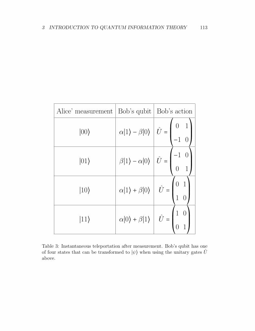
3 INTRODUCTION TO QUANTUM INFORMATION THEORY 113

Alice’ measurement Bob’s qubit Bob’s action

∣00⟩ α∣1⟩ − β∣0⟩ U =⎛⎜⎜⎝

0 1

−1 0

⎞⎟⎟⎠

∣01⟩ β∣1⟩ − α∣0⟩ U =⎛⎜⎜⎝

−1 0

0 1

⎞⎟⎟⎠

∣10⟩ α∣1⟩ + β∣0⟩ U =⎛⎜⎜⎝

0 1

1 0

⎞⎟⎟⎠

∣11⟩ α∣0⟩ + β∣1⟩ U =⎛⎜⎜⎝

1 0

0 1

⎞⎟⎟⎠

Table 3: Instantaneous teleportation after measurement. Bob’s qubit has oneof four states that can be transformed to ∣ψ⟩ when using the unitary gates Uabove.

3 INTRODUCTION TO QUANTUM INFORMATION THEORY 114

If Alice measures her two qubits and sends to Bob her result via a classicalchannel, then Bob can restore the original state ∣ψ⟩ when using the unitarygates given in Table 3. For example, if the measurement result is ∣00⟩, Bob’squbit is (−β,α)T , and applying U yields the desired state (α,β)T . The originalstate ∣ψ⟩ is destroyed, which is in agreement with the No-Cloning Theorem.

So far, so good, and in almost all text books (at least that I have read) theinterpretation is that there are fortunately no conflicts and no paradoxes withthe theory of relativity, because we have a complete teleportation only whenthe two final bits from the measurement are send from Alice via a classicalchannel to Bob. This can be done only with a velocity not larger than thespeed of light. OK, then it seems that it doesn’t matter that in a quarter of allcases an instantaneous teleportation has happened without sending two bitsfrom Alice to Bob.

The statement that teleportation does not violate the theory of relativity,however, is not always shared. One exception can be found in the well-knownbook of Penrose52 in Chapter 23.9. His scenario was that he had to send thestate ∣ψ⟩ to his colleague who stays on Titan 5 light years away. He writes:

Yet, we shall find this direction leading into a territory thatmany people would, no doubt, be most reluctant to enter- and withreason as we shall see. [...] What is particularly striking aboutquantum teleportation is that, by sending my colleague 2 bits ofclassical information (one of the numbers 0,1,2,3,4, which couldhave been coded as 00, 01, 10, 11, respectively), I have conveyedthe ’information’ of a point on the entire Riemann sphere [...] theinformation contained in the unrestricted choice of a point in a con-tinuum: strictly ℵ0 bits, for perfect accuracy! At this point I shouldmention that real experiments have been performed which confirmthe expectations of quantum mechanical exportation (over distancesof the order of metres, not Earth-Saturn spans, of course) so wemust take these things seriously. Not only that, but the blossomingsubject of quantum cryptography depends upon things of this gen-eral nature; so do many ideas of quantum computation. Penrose2004

Penrose displayed a spacetime diagram, see Figure 68. It describes a linkbetween the state ∣ψ⟩ before teleportation and after teleportation. But thispath goes 5 years back into the past. We shall come back to this apparentconflict later.

52Penrose, Roger. The Road to Reality: A Complete Guide to the Physical Universe.Jonathan Cape, 2004.

3 INTRODUCTION TO QUANTUM INFORMATION THEORY 115

'

&

$

%

Alice Bob

|ψ

|ψ

classical channelafter5 years

Start

Bell pair created12

(|01 - |10)

Figure 68: Penrose’s spacetime diagram for quantum teleportation shows theacausal propagation of quantum information ∣ψ⟩. The unknown superposedquantum state ∣ψ⟩ with its ℵ0 bits is with certainty teleported by simply send-ing 2 bits of classical information. In a quarter of all cases, however, an in-stantaneous teleportation occurs without sending classical information. Thereseems to be something completely wrong, in quantum mechanics or in relativ-ity theory or in both. Nevertheless there is a link in the spacetime diagram, thedotted path. Unfortunately, this path goes 5 years back into the past leadingto an acausal propagation of quantum information.

4 UNIFICATION VIA SEMIMODULES 116

4 Unification via Semimodules

Based on our previous description of reversible, random, and quantum compu-tation, we present a unification of physical concepts such as states, observablesand dynamics. In the literature these notions are defined in different ways de-pending on the physical theory. This unification, independent of the physicalmodel, makes use of semimodules. A semimodule is a linear space where thefield of numbers is replaced by a number system without requiring subtrac-tion and division. It turns out that the weird quantum principles presentedin Section 1 actually are very natural and coincide with what we feel and ob-serve. In particular, we describe quantum mechanics as a probabilistic theoryof possibilities that characterize the future. This theory applies just as well tomacroscopic objects. The central goal of this section is to show variousconsequences when we replace the external parameter time t by atrinity, namely the partitioning future, present, and past. Clearly,then spacetime vanishes. However, among many other consequences, we showan alternative approach to the Lorentz transform, the key to the theory ofrelativity. Additionally, we discuss the dimensions of the underlying spaces indifferent physical theories. From the point of view of information theory weinvestigate in which dimensions a physical theory could be reasonable.

4 UNIFICATION VIA SEMIMODULES 117

4.1 Preliminaries

In the introduction of these lecture notes we displayed the strange principlesof quantum physics. If we look in more detail into physics, it turns out thateven basic concepts become very vague. When asking what a state in physicsis, one cannot find a simple answer. For example, on the page ”Physics StackExchange“ in December 2015, the following question occured:

What is a state in physics? While reading physics, I have heardmany a times a ”system is in ... state“ but the definition of astate was never provided (and googling brings me totally unrelatedtopic of solid state physics), but was loosely told that it has everyinformation of the system you desire to know. On reading further,I have found people talking of Thermodynamic state, Lagrangian,Hamiltonian, wave-function etc etc which I think are different fromone another. So in general I want to know what do we mean bystate in physics and is there a unique way to describe it? ManishKumar Singh53

The last question is really important and seemingly difficult to answer.Such questions show on the one hand a great interest in science, but on theother hand they exhibit insufficient explanations of basic physical concepts inmany textbooks.

It is common sense that each physical theory must work out three funda-mental tasks:

1. States must be defined.

2. All possible outcomes or observable values of an experiment must bespecified precisely.

3. The dynamics, which allows to predict a future state given the currentstate, must be presented. In other words, we need a rule about howstates change with time.

In physics the concept of a state and the notion of an observable is some-times presented ambiguously. Most physicists say that the precise definition ofa state depends on the underlying physical theory. We look at some examples:

• In classical mechanics, the space of states can be the six-dimensionalphase space, the four-dimensional spacetime, or discrete subsets due tosome coarse graining. For a system of n particles the phase space isR6n, three spatial coordinates and three coordinates for the momentumof each particle. In all cases states are points in a real space.

• In quantum mechanics, a state is an element of a complex Hilbert space.Each state is a superposition of base states. The base states form anorthonormal basis of the underlying Hilbert space. For example, the

53 see Physics Stack Exchange, December 2015, http://physics.stackexchange.com/questions/223564/what-is-a-state-in-physics

4 UNIFICATION VIA SEMIMODULES 118

base states of a polarized photon are described by its polarization angleα and two possibilities, namely vertical and horizontal polarization. Thebase states of an electron are described by its momentum and its spin.

• In classical probability theory the set of states is the sample space, whichis defined as the set of all possible outcomes of a random experiment. Theoutcomes are also called elementary events. Events are specific subsetsof the sample space.

• The formalism of thermodynamics and statistical physics can be devel-oped classically, but also in terms of quantum mechanics. There, systemsof a very large number of particles are considered. In the absence of in-teraction, each particle can be in one of its possible states, a classicalor a quantum one. The realization where each particle is in a certainstate i is called a microstate of the system. The information given bymicrostates is excessive. A compressed meaningful information is thenumber of particles that are in state i, say Ni. These numbers specifythe macrostates in thermodynamics.

• More subtle is the definition of states in quantum field theories.

Summarizing, we have a colorful diversity of concepts for the definitionof a state. Moreover, the states of classical mechanics and of quantum me-chanics seem to differ significantly. For instance, in the book of Susskind andFriedman54 we find:

In Volume I, it took a little more than a page to explain whata state is in classical mechanics. The quantum version has takenthree lectures, three mathematical interludes, and according to myrough count, about 17,000 words to get to the same place. But Ithink the worst is over. We now know what a state is. Susskindand Hrabovsky 2013

There seems to be little hope to find a short, precise and all-encompassingdefinition of a state, independent of the underlying physical theory. Closelyrelated is the problem to find a universal valid definition of an observable. Inthe following we will elaborate on these concepts in detail.

At least as difficult seems to be the interpretation of the mathematicalformalisms that describes a physical theory. In this context Peres says that ina laboratory an experimental set up consist of various machines that produceoutputs in terms of color, current, voltage, tension and so on. These measuredoutputs are described by numbers, and he writes:

Some authors state that the last stage in this chain of mea-surements involves ”consciousness,” or the ”intellectual inner life”of the observer, by virtue of the ”principle of psycho-physical par-allelism.” Other authors introduce a wave function for the entire

54Susskind [2014], page 93

4 UNIFICATION VIA SEMIMODULES 119

universe. In this book, I shall refrain from using concepts that I donot understand. Peres55 1995.

About the difference between conclusions, such as many mind interpretationsderived from the mathematical formalism, and the reality he says:

Quantum phenomena do not occur in a Hilbert space. Theyoccur in a laboratory. Peres56 1995

Like Peres we try to avoid any weird concepts which are difficult to under-stand, if at all. This includes even the widely used concept of an observer.

55 Peres [1995], pages 25-2656Peres [1995], page 373

4 UNIFICATION VIA SEMIMODULES 120

4.2 Base States

All physical theories are based on experimental set-ups or machines that arecharacterized by a fundamental property, namely the existence of mutuallyexclusive and empirically decidable alternatives. We postulate this property,since a theory without alternatives is hardly imaginable. We call these alter-natives in the following base states. Let us look at some examples.

In classical mechanics dynamical variables, like position, momentum, orenergy provide alternatives for describing the freedom of a particle or of aphysical system. For example, a particle can be in this or that position, butnot simultaneously in several positions. In the same way the particle canoccupy one of many different geometrical objects. For instance, a harmonicoscillator may be on one of the orbits in phase space. In a slit experiment thebase states are the different positions at the wall of detectors.

In classical probability theory outcomes, also called elementary events, arethe base states. They are the alternatives that define the sample space. For acoin the base states are Head and Tail. For a dice the base states are 1,2,3,4,5,and 6. For a slit experiment the base states are the positions at the wall ofdetectors. When detectors are added at the slits, then the base states are pairsof detectors. The first element of this pair contains the detected position, andthe second element contains the located slit. The base states are the same asin classical mechanics, only their names differ.

The same definition of base states applies to quantum mechanics. As be-fore, the positions define the base states in a slit experiment. In optics, aphoton passing a calcite polarizer has the possibility to be in one of two beamswith perpendicular polarization, yielding two base states, namely horizontaland vertical polarization.

In thermodynamics, the base states are the microstates or the macrostates,depending on whether we consider the microscopic or the macroscopic model,respectively.

In some field theories, the base states are the classical fields, namely thesolutions of classical field equations.

Keep in mind: For any physical theory we postulate the existenceof mutually exclusive alternatives, the base states. A theory withoutbase states is hardly imaginable.

Now we have a precise definition of base states as alternatives, that is,mutually exclusive distinguishable situations. This definition applies to allwell-known physical theories. But how can we represent base states? Look-ing at the previous examples it follows that base states can be represented bynumbers. For a dice or a coin toss the base states are natural numbers. Simi-larly, the base states of other physical models can be represented, at least bygrouped numbers. In summary, any experimental set-up can be characterizedby a collection of numbers that have a specific meaning in the experimentalcontext. We call this the number representation of base states. It is the mostcommonly used representation in physics.

4 UNIFICATION VIA SEMIMODULES 121

Additionally, there are two other mathematically equivalent representa-tions. Any number can be represented as a string of bits, called register.Commonly, a bit is defined as a quantity that can only take one of two val-ues 0 and 1. It is the basic unit in information theory. The two values areinterpreted as logical values TRUE or FALSE. Thus, in addition to the num-ber representation we have an equivalent register representation of base states.The register representation is the most commonly used representation in in-formation theory.

In the following, we consider only systems with a finite number N of basestates, or at most a countable set of base states. The N registers representingall base states can be expressed equivalently as the orthonormal standard unitvectors in CN . We call this the vector representation of base states, and thetransition from the number representation or the register representation tothe vector representation is called vectorization. The vector representation iswidely used in quantum theory, when working with bits and qubits.

Frequently, in these notes our interpretation of a bit is as follows:

• A bit is a question at a system that has exactly two possible answers,say YES for 0 and NO for 1.

For certain systems the base state can be represented by a register consistingof a sequence of binary questions. In such situations we obtain a better insightinto certain physical relationships. Then a register of n bits can be representedequivalently as a standard unit vector in C2n via the tensor product of the bitsin the register. This vector representation is widely used in quantum theory.

The four numbers 0,1,2,3 have the register and vector representations

∣00⟩ =⎛⎜⎜⎜⎝

1000

⎞⎟⎟⎟⎠, ∣01⟩ =

⎛⎜⎜⎜⎝

0100

⎞⎟⎟⎟⎠, ∣10⟩ =

⎛⎜⎜⎜⎝

0010

⎞⎟⎟⎟⎠, ∣11⟩ =

⎛⎜⎜⎜⎝

0001

⎞⎟⎟⎟⎠. (198)

We use as before Dirac’s bracket notation for representing states.Summarizing, we have three mathematical equivalent representations of

base states: the number, register, and vector representation. This has someimportant consequences, as we will see later. Among them are consistent def-initions of states and observables for various physical models, a vectorizedclassical mechanics, or a unified treatment of classical mechanics, classicalprobabilistic mechanics, and quantum theory via semimodules. In the litera-ture quantum mechanics is presented as a linear theory in contrast to classicalmechanics. But it turns out that a vectorized classical mechanics is a lineartheory as well, working with permutation matrices, a special class of unitarymatrices.

4 UNIFICATION VIA SEMIMODULES 122

Keep in mind: The mutually exclusive alternatives, the basestates, can be described in terms of three mathematical equiva-lent representations. The number representation that is well-knownfrom classical theories. The register representation that is fre-quently used in information theory. For certain systems this repre-sentation shows the divisibility of physical knowledge into decidableYES / NO questions. Finally, the vector representation that is usedmainly in quantum theory. In particular, classical mechanics hasalso a vector representation, and thus can be viewed as a linear the-ory. In the same way quantum mechanics has a number represen-tation, for instance, the componentwise Schrodinger equation. Wemake use of all three representations. A major reason that physicaltheories seem to be incompatible or inconsistent sometimes goesback to the ignorance of these equivalent representations.

A first important consequence is the distinguishability of base states. Inclassical mechanics two base states, such as position or momentum, with differ-ent number representations are called distinguishable. In quantum mechanicswe have to learn the seemingly strange definition that only orthogonal statesare distinguishable. It follows that the notion distinguishability seems to de-pend on the physical theory. Actually, it does not depend on the physicalmodel, but on its representation. We have the obvious natural equivalences:

• Two base states i and j in their number representation are distinguish-able if their numbers are different. ⇔

• Two base states in their register representation are distinguishable iftheir registers i = (i0, ..., in) and (j = j0, ..., jn) are different. ⇔

• Two base states in their vector representation are distinguishable if theircorresponding standard unit vectors ∣i⟩ and ∣j⟩ are orthogonal, that is,

⟨i∣j⟩ =n−1

∑k=0

ikjk = 0. (199)

The latter property follows because different register representations imply dif-ferent orthogonal standard unit vectors. Orthogonality and distinguishabilityof base states are exactly the same, only expressed in different representations.

In order to get a feeling for the above notions, we consider the exampledisplayed in Figure 69. It has only six base states. This is sufficient forour purposes, since most of the conceptual issues have nothing to do with aninfinite number of base states.

In this example a circuit is chopped into a collection of six cells that areconsecutively represented in terms of numbers, namely their correspondinghalf-open intervals of angles:

∣[0, π3)⟩, ∣[π

3,2π

3)⟩, ∣[2π

3, π)⟩, ∣[π, 4π

3)⟩, ∣[4π

3,5π

3)⟩, ∣[5π

3,0)⟩. (200)

4 UNIFICATION VIA SEMIMODULES 123

'

&

$

%

right

left

Figure 69: A circuit is chopped into a collection of 6 cells by bisection threetimes the circuit. A point x is positioned on the circumference. For eachline bisecting the circuit we can ask the question whether point x is on theright or on the left side of the line yielding the value 0 or 1, respectively.Hence, each cell with the number representation ∣[kπ3 ,

(k+1)π3 )⟩ has an equivalent

register representation ∣i0, i1, i2⟩ with i0, i1, i2 ∈ {0,1}, thus an equivalent vectorrepresentation. They represent the 6 cells. This example requires 3 binaryalternatives yielding 6 base states where a specific point x may be positioned.

Of course, we could make the cells arbitrarily small, but leave the number ofbase states finite. Then nothing would change the following considerations.

In many cases, we use for each representation sometimes Dirac brackets inorder to keep in mind the fundamental vector representation. This will causeno ambiguities.

We obtain the register representation as follows: we start with the linethrough 0 and π, and ask whether a fixed specific point x is on the right sideor on the left side of this line, when looking from 0 to π. If x is on the rightside we write a 0, and otherwise we write a 1. Then we take the line throughπ/3 and 4π/3 and ask the same question. Finally, we take the line through2π/3 and 5π/3 and ask this question once more. Since we have only six basestates representing the mutually exclusive cells and 6 ≤ 23, we need only threequestions that yield a 3-bit register representation.

Obviously, the point x displayed in Figure 69 is in the cell ∣[π3 ,2π3 )⟩, which

4 UNIFICATION VIA SEMIMODULES 124

has the number, register and vector representation

∣[π3,2π

3)⟩ = ∣001⟩ = (01000000)T ∈ C8, (201)

respectively. Here, we have represented a register of 3 bits (questions) as astandard unit vector in C8 via the tensor product of the bits in the register.The representations of the other cells are displayed in the same figure. If onepoint is positioned on the circuit, it is in exactly in one of these six non-overlapping cells. Mathematically, these alternatives form an orthonormal setof canonical unit vectors in C8, when using the vector representation. Thisjustifies the name base states.

In our example, the registers ∣101⟩ and ∣010⟩ do not occur, since bothare impossible when interpreting the related bits as questions. We can avoidsuch impossible registers when we switch to C6, which can be viewed as asubspace of C8. It is interesting that there are examples where impossibleregisters do not occur. If we bisect the circuit only two times, then we obtain4 = 22 registers that only represent possible base states. Impossible ones donot occur. Another example is a sphere in the three dimensional real spacewhere an axis passes through the center of the sphere. The plane through thecenter orthogonal to this axis divides the sphere into two halves, and we canask the question on which half a point may be positioned. This gives the firstbit. Then we rotate the axis. This gives a new plane, and we can ask the samequestion yielding a second bit. Then we rotate once more and obtain a thirdbit. The 23 corresponding 3-bit registers represent base states where a pointpossibly may be positioned on the sphere. Taking more than three planesleads to impossible base states. In general, we can always avoid impossiblebase states by passing to an appropriate subspace.

Another aspect is that these representations are ambiguous, as usual inphysics. In the number representation, for instance, we could simply write thenumbers 1 to 6. In the register representation, we can interchange 0 and 1 foreach bit.

This example can be used in various physical models and situations, some ofthem are described below. Although it has nothing to do with small particles,we shall see later that it generates the mathematical formalism of quantummechanics. Let us think of a point as a soccer ball, and think of the circuit asa large hula hoop. Then the cells are an appropriate partitioning of the hulahoop, and we have a simple macroscopic example.

(A) We can number the six base states from 1 to 6 as above yielding anothernumber representation. This set of numbers can also be viewed as thesample space of a dice. The states are called outcomes in classical proba-bility theory. In particular, it follows that these outcomes have a naturalregister representation as well as a vector representation. Usually, bothrepresentations are not exerted in classical probability theory.

(B) In terms of classical mechanics this example may describe one particleon some position x on the circuit. The classical states of this particle are

4 UNIFICATION VIA SEMIMODULES 125

the possible positions given by the cells. The cells are the base statesthat have a number, register, and vector representation. More general,the theory of classical mechanics can be described equivalently in one ofthese three representations, but only the number representation is widelyused. Sometimes it is advantageous to describe classical mechanics in itsvector representation.

(C) Classical fields can be described as well. Suppose we want to measure thetemperature in a room with a circuit wall. In each cell we have placed anair thermometer at the wall. The temperature in each cell can be writtenapproximately as a finite register, say with 5 bits. One realization of aclassical field could be

cell 011 temperature 10100cell 001 temperature 10011cell 000 temperature 10010cell 111 temperature 10001cell 110 temperature 10011cell 100 temperature 10010

(202)

When we merge consecutively the bits of this field, we obtain its registerrepresentation

∣i⟩ = ∣011 10100 001 10011...⟩. (203)

In a field theory the possible fields ∣i⟩ of the form (203) define the basestates.

(D) The idea of thermodynamical microstates and macrostates can be ex-plored in our simple example as follows. Suppose we have 6 chips, blackon one side and red on the other. We toss them and place them in the 6cells. A microstate is a list of 6 elements with a color on each side. Themicrostates form a set of base states that can binary be represented with0 for black and 1 for red. This gives their register representation. Inour case there are 64 microstates that are equally likely with probability1/64 for each one.

A macrostate is characterized by the total number of black coins, sincethe others are red. If this number is 1, for example, then 6 microstateshave this property and the probability of this macrostate is 6/64. Themacrostates form a set of base states that may be labeled as

∣0⟩, ∣1⟩, ∣2⟩, ∣3⟩, ∣4⟩, ∣5⟩, ∣6⟩.

(E) We can use this model for describing the dynamics of particles. Fermionscan be viewed as soccer balls such that at most one of them is in each cell.If a particle is in a certain cell we write a 1, otherwise we write a zero.Hence, a base state is a 6-bit register, for instance ∣100110⟩. In its vector

4 UNIFICATION VIA SEMIMODULES 126

representation it is a standard unit vector in C26 . This toy model allowsus to work with a variable number of particles. It is closely related toa Fock space in quantum field theory. Particles may be annihilated. Forexample, the base state ∣100110⟩ may change to ∣000110⟩. The vacuumis defined as the space without any particles, that is, the base state∣000000⟩. The vacuum is mathematically represented as the standardunit vector ∣000000⟩. This vector has in the first component a 1 andotherwise zeros. It represents our hula hoop without soccer balls. Theannihilation operator maps the vacuum onto the zero vector, since thereis no particle that can be annihilated. In reverse, we can create particlesin specific cells that contain no particle. If we want to create a particlein a cell which is already occupied, the creation operator maps this basestate onto the zero vector since each cell can contain at most one fermion.In particular, a creation operator maps the base state ∣111111⟩ alwaysonto the zero vector.

Bosons have the property that any integer number of particles can be inone cell. Also in this case we can create and annihilate particles. Butnow the creation operator does never map a state onto the zero vector.Notice that the creation and annihilation operators act on base states.

Keep in mind: Given a machine or any experimental set-up. Itsbase states are the mutually exclusive alternatives. Two base statesare different and distinguishable, if and only if

(i) in the number representation the corresponding numbers arenot equal,

(ii) in the register representation the corresponding registers arenot equal, and

(iii) in the vector representation the vectors are orthogonal.

4 UNIFICATION VIA SEMIMODULES 127

4.3 Irreversibility and Trinity of Time

A major goal of these lecture notes is to describe how physics might work with-out an external time parameter t and a (3+1)-spacetime. This is a radicallydifferent entrance to physics. We completely avoid to use a real time variablet. At a first glance, it seems that most physical theories must vanish: no clas-sical theories like electromagnetism, no special or general relativity theory, noquantum field theories, and no particle physics. Actually, the mathematicalformalisms of these theories can be recovered, but the interpretations changedrastically. It turns out that it is possible to formulate physics as a timelesslanguage without apparent paradoxes, but with unified definitions of states,observables, and the change of states.

Firstly, we need to consider some aspects of the nature of time, perhapsthe deepest of all philosophical puzzles. Newton believed that absolute timeexists independently of other influences. Mathematically, it means that timeappears as an external parameter in the equations of motion characterizingthe temporal development of a physical system.

Many physicists and philosophers thought about time and came to diversedefinitions. One of the most radical consequences in the theory of relativityis that any moving clock slows down relative to a stationary observer. Thisphenomenon is called time dilation. Moreover, the relativity of simultaneity,that is, whether two spatially separated events occur at the same time, dependson the observer’s reference frame, thus is not absolute.

Although quantum theory is unified with special relativity in relativisticquantum theory, the meaning of time becomes even more strange in generalrelativity. This results in the well-known problem of quantum gravity whentrying to unify quantum theory with general relativity. One way to deal withthis problem is a well-known standard recipe with which one can generate asuitable quantum theory from a Hamiltonian formulation. Applying this recipeto general relativity leads to the Wheeler-de Witt equation (we cannot go intodetails), formally written as HΨ = 0, where Ψ is the wave function of theuniverse, which depends on the geometry and the matter content of the entirespace-time. The crucial point is that this equation does not involve any time.It is static and thus has generated much controversial discussions. This is notvery surprising, however, since even general relativity theory does not containa separate time parameter, but describes the entire spacetime as a variable.

Is a quantity t with such strange properties a time or an illusion? However,it seems to be hardly possible to define fundamental physical terms absoluteexactly. Feynman wrote in his famous Feynman Lectures Volume I, 8-1:

We can’t define anything precisely. If we attempt to, we getinto that paralysis of thought that comes to philosophers ... onesaying to the other:”you don’t know what you are talking about“.The second one says: ”what do you mean by talking? What do youmean by you? What do you mean by know?”

We try, nevertheless, to define several physical terms as accurately as pos-sible, and in accordance with language, experience, and experiments. If we

4 UNIFICATION VIA SEMIMODULES 128

'

&

$

%

PRESENToutcomes

classical probability theory

PASTfacts

classical mechanics

FUTUREpossibilities

quantum mechanics

Feynman rules

collapse

action S

amplitudes eiħ S

IRREVERSIBLETRINITY

Figure 70: Trinity of time. Go through the slit experiments with this picturein mind.

have an experience about time at all, then of course not about an externaltime parameter. But it is obvious to everyone that our experiences show thatall phenomena behave irreversible, and moreover we observe a trinity of time” future, present, and past”. These experiences are unmistakable and notdisproved by any experiments.

The irreversibility in our world exhibits for instance in the observation that”broken cups do not fit together by themselves”. Another funny demonstrationis to run a film backwards.

The past is fixed. It is characterized by the things that happened, that wedo remember, thus by facts that exist, that are unique, that are determined,that perhaps we know or that are measured by any machine. The future isopen, is characterized by all things that might happen, that is, by possibilities.Between future and past is the present. The present is neither an instant oftime nor a time interval. It describes what actually happens, that is, it selectsfrom a set of possibilities exactly one outcome which then in turn becomes afact in the past.

This trinity is deeply rooted in our behavior, our thinking, our language,our genetics. Perhaps, even Neanderthalers, or even animals, have this expe-rience. This trinity, which may be visualized as a tripartite circle as displayedin Figure 70, forms a basis of this lecture notes.

Perhaps a very very naive but helpful picture is a pinball machine. If thismachine is built, there are a lot of possible games and results. These are the

4 UNIFICATION VIA SEMIMODULES 129

possibilities one has in the future. When you play a game you are in thepresent. When the game is over the result is a fact in the past. The past caninfluence the future. Perhaps you have won some additional games.

Keep in mind: Our experience of future, present, past, and ir-reversibility is deeply rooted in our behavior, our thinking, ourlanguage, our genetics. Physics can be formulated on the basis ofthis experience as a timeless language without apparent paradoxes,but with unified definitions of states, observables, and the changeof states. A major goal of this lecture notes is to describe physicswithout an external time parameter in a simple manner from thevery beginning, and thus supporting the Wheeler-de Witt equationderived formally from a Hamiltonian formulation of general relativ-ity.

4 UNIFICATION VIA SEMIMODULES 130

4.4 States

Above, we have replaced time by the trinity future, present, and past. More-over, we have introduced a common unique notion of base states as mutuallyexclusive and empirically decidable alternatives which are suitable for describ-ing several different physical models. But what is a state? At the beginning ofthis chapter we have seen that in the literature states are defined in differentmanners depending on the physical theory. Now, using our definition of basestates we can unify the idea of a state.

Given a machine or an experimental set-up which is characterized by a setof base states {∣i⟩}. A state is defined as a (probabilistic) superposition of basestates

∣ξ⟩ =∑i

ξi∣i⟩, ξi ∈ S, ∑i

∣ξi∣2 = 1, (204)

where S is a number system, see Section 2.2. In the following we classifystates according to the three number systems: the non-negative integers N,the non-negative real numbers R+, and the complex numbers C.

Firstly, let us consider two-state systems that is, we look at binary alter-natives. These systems correspond to single bits, that is, YES/NO questions.

A

⎧⎪⎪⎪⎨⎪⎪⎪⎩

classicalrandomquantum

⎫⎪⎪⎪⎬⎪⎪⎪⎭state , short form is

⎧⎪⎪⎪⎨⎪⎪⎪⎩

bitrbitqubit

⎫⎪⎪⎪⎬⎪⎪⎪⎭, (205)

is represented in the form

∣ξ⟩ = ξ0∣0⟩ + ξ1∣1⟩ = (ξ0

ξ1) ∈

⎧⎪⎪⎪⎨⎪⎪⎪⎩

N2

R2+

C2

⎫⎪⎪⎪⎬⎪⎪⎪⎭, (206)

where

∣0⟩ = (10) , ∣1⟩ = (0

1) , (207)

and the coefficients satisfy the normalization condition

∣ξ0∣2 + ∣ξ1∣2 = 1. (208)

The meaning of the coefficients is related to the number system. In a certainsense, however, they have a probabilistic meaning.

For integer coefficients we obtain the classical states. The normalizationcondition implies that either ξ0 = 1, ξ1 = 0 or ξ0 = 0, ξ1 = 1. Hence, the onlystates are the base states, either zero or one. This definition coincides withthe definition of a classical bit in Section 3.3. Bits represent facts, things thathave happened. Facts describe the past. When a coin is thrown, for example,it shows either Head or Tail. When a particle has passed an interferometer,

4 UNIFICATION VIA SEMIMODULES 131

it interacts exactly with one detector. The past is deterministic. Neverthe-less, the coefficients ξ0 and ξ1 of a classical bit can be viewed as ”extremeprobabilities”, where exactly one has the value 1 and the other is 0.

For random states the coefficients ξ0 and ξ1 are nonnegative, and theirsquares sum up to one. These squares ∣ξ0∣2 and ∣ξ1∣2 represent the correspondingprobabilities for the two outcomes of the random bit. Here we have definedrandom states in a way such that the coefficients must be squared in order toobtain the classical probabilities. At a first glance, it would be better to definerandom states as usual in the form

∣ξ⟩ = ξ0∣0⟩ + ξ1∣1⟩, ξ0 + ξ1 = 1, ξ0, ξ1 ≥ 0. (209)

But then we must change the normalization condition. Because there is uniquecorrespondence between positive numbers and their squares, it is more appro-priate to maintain the normalization condition and to use Born’s rule for thesquare roots of classical probabilities. Then the definition of squared randombits coincides with the definition of a random bit in Section 3.5.

Random states describe experimental outcomes that happen at this mo-ment, that is, in this moment the two-state system collapses to one base state∣0⟩ or ∣1⟩, respectively. Random states represent the present. We call the tran-sition from the present to the past and from classical probabilistic outcomes tofacts the collapse. In a coin toss either Head or Tail emerges. In experimentswith an interferometer exactly one detector clicks. In a slit experiment ex-actly one of the position detectors at the wall clicks. In this interpretation thecollapse is not a second dynamics in quantum theory as pointed out in the lit-erature. Instead it happens when going from the present (classical probability)to the past (classical mechanics). This transition is irreversible. We cannot goreversely from the past (unique facts) to the present (several outcomes).

For quantum states the coefficients ξ0 and ξ1 are complex numbers, theso called probability amplitudes. Squaring their magnitudes gives the classicalprobabilities for outcomes. The definition of quantum bits coincides with thedefinition of a quantum bit in Section 3.6. The obvious difference to classicalprobabilities are that complex amplitudes are numbers that allow cancellationor interference, in contrast to non-negative numbers.

Quantum states represent the future in terms of ”as well as” distinguishablepossibilities. The transition from the future to the present and from quantumprobabilistic outcomes to classical probabilities is given by Born’s rule, namelyto square the magnitudes of complex amplitudes. In this interpretation Born’srule is applied when going from the future (quantum amplitudes) to the present(classical probability). This transition is likewise irreversible. Due to thesquaring procedure, we cannot go reversely from the present to the future.But the other way around works. The facts of the past affect the possibilitiesof the future. Changed facts offer new possibilities. A cup must be producedat first. If this is done it belongs to the past. Only then one has the mutuallyexclusive possibilities to fill the cup with water, tee, or coffee. In this sense weget an irreversible circle of future, present, and past, as displayed in Figure 70.

In physics the arrow of time expresses our observed one-way property oftime, although almost all equations are reversible with respect to time. The

4 UNIFICATION VIA SEMIMODULES 132

British astronomer Eddington introduced this concept 1928, and, using severalarguments, he concluded that the time’s arrow is a thermodynamical propertyof entropy alone. Physical processes at the microscopic level, however, arebelieved to be reversible in time. More precisely, if we reverse the direction oftime all mathematical statements remain true. Our approach is fundamentallydifferent. Firstly, we have no time t, hence, we cannot reverse its direction.Secondly, we have a circle representing the trinity, not an arrow. In particular;the circle is closed such that our experience ”facts influence the future” isincorporated. That physical quantum processes at the microscopic level arereversible can be simply resolved in our treatment of the trinity of time. Wedescribe quantum theory in terms of as future actions or possibilities andreversible unitary transformations that map base states onto base states.

The same mathematical formalism applies not only to two-state systems,but also to multi-state systems. These systems can be represented as registers

i = (i0 . . . in−1), ij ∈ {0,1} (210)

with vector representation ∣i⟩. A

⎧⎪⎪⎪⎨⎪⎪⎪⎩

classicalrandomquantum

⎫⎪⎪⎪⎬⎪⎪⎪⎭state or register

is a superposition ∣ξ⟩ of base states ∣i⟩:

∣ξ⟩ =∑i

ξi∣i⟩ =⎛⎜⎝

ξ0

⋮ξN−1

⎞⎟⎠∈⎧⎪⎪⎪⎨⎪⎪⎪⎩

NN

RN+

CN

⎫⎪⎪⎪⎬⎪⎪⎪⎭. (211)

with vectorized base states

∣i⟩ = ∣i0, ..., in−1⟩, (212)

satisfying the normalization condition

∑i

∣ξi∣2 = 1.

The meaning of the coefficients is exactly the same as for two-state systems.

Keep in mind: Base states are non-overlapping, distinguishablealternatives that define the facts in the past, the outcomes or ele-mentary events in the present, and the distinguishable possibilitiesof the future. They do not change when going from the future tothe present and then to the past. This is important and is in con-trast to states. They are defined as superpositions of base statesand differ with respect to the trinity of time: in the past we haveclassical states, in the present we have classical probabilistic states,and in the future we have quantum states.

4 UNIFICATION VIA SEMIMODULES 133

4.5 Some Experiments Revisited

In this section we explain the notions base states, states and possibilities interms of some examples.

Let us first consider a fair die. Its base states are the numbers 1,2,3,4,5,6.They define the outcomes before we toss the die, and exactly one of thesenumbers becomes a fact if the die is tossed. In this simple example we can alsosay that the base states provide six distinguishable possibilities. In the future,when the die is not yet tossed, we can assign probability amplitudes ±1/

√6

to the base states. They are not uniquely defined. When we toss the coin inthe present, then each base state has the probability 1/6. This follows fromBorn’s rule. The present is best described by the classical probability rules ofKolmogorov. In this theory probabilities are non-negative numbers such thatinterference cannot occur. Probabilities of mutually exclusive events are addedand probabilities for independent events are multiplied, the same rules as forprobability amplitudes. Finally, when the die is tossed one of the six numbersbecomes a fact.

Next, we consider Renninger’s negative-result experiment, where around alight source two spherical scintillation screens with different radii are placed,see Figure 34. The outer radius is very large compared to the inner radius. Thelight source emits in sufficiently large ”time intervals” a photon that can movein all directions. It was designed to show that knowledge is gained, althoughnot any detection has happened.

In our approach, given the experimental set-up without any emitted pho-ton, we calculate the probability amplitudes for the two future actions: thephoton is detected at the inner or at the outer screen. These are all basestates. The probability amplitudes are not uniquely defined, but their squaredmagnitudes must correspond to the areas of both screens. The experimentalset-up determines completely the probabilities, the only quantities that can bemeasured. When a photon is emitted in the present, then each base state hasvia Born’s rule a probability related to the area. Finally, when the photon isdetected, one of the base states becomes a fact. That settles the experiment.Since we have no time parameter, we have no time-dependent wave-function,and we cannot gain any knowledge. Nothing strange happens. It is a shortexercise to explain in the same way Schrodinger’s cat.

Some important aspects occur when we look at slit experiments. Supposethat the experimental set-up is given, but no particle is in the experiment.Hence, we ask what might happen in the future. There are several possibilitieswhere a particle can go from the source s through some hole i in the first wall,then through some hole j in the second wall, and finally to a detector x at thescreen. The corresponding amplitude related to this possibility or path is

⟨x∣j⟩⟨j∣i⟩⟨i∣s⟩. (213)

We know already that these probability amplitudes depend on the geometryof the experimental set up, and can be calculated easily. Our next questionis: what are the base states? It seems to be natural to identify the base stateswith the possible paths. But this would not work, since the paths are not

4 UNIFICATION VIA SEMIMODULES 134

distinguishable, provided we have no detectors at the slits. The particle canmove in a future action on this path as well as on any other path from sources to detector x. What are the mutually exclusive alternatives? These are thepositions. At the screen exactly one detector would observe a particle. Thus,the positions form distinguishable, non-overlapping outcomes. The amplitudesfor these outcomes ⟨x∣s⟩ are calculated as follows: the amplitude to arrive fromsource s at a specific position x is a sum of all amplitudes:

⟨x∣s⟩ = ∑i=1,...,Nj=1,...M

⟨x∣j⟩⟨j∣i⟩⟨i∣s⟩. (214)

The single amplitudes (213) in this superposition correspond to the variousnon-distinguishable, but mutually exclusive possibilities. In particular, possi-bilities have not the property that either this or this may happen, as is truefor outcomes. Possibilities are in general non-distinguishable elements of thefuture, where nothing happens. Thus, one possibility as well as other pos-sibilities lead to the same outcome (base state) described by formula (214).In other words, possibilities form a set of decisions or paths that may be notdistinguishable, in general. Base states are the distinguishable possibilities.However, in some models as in the previous examples the possibilities maycoincide with the base states.

In order to obtain the correct probabilities in experiments we have to definethe base states very carefully. Moreover, we should have in mind that a basestate represents a possibility, but not reversely. When we have additionallydetectors at all slits, then the paths (possibilities) through the various slitsare distinguishable and become base states. Thus we obtain a completely newand larger set of base states, leading to another probability distribution. Inparticular, interference vanishes. We have discussed these aspects extensivelyin Section 2.6, and we have seen that the slit experiment is not strange orparadox.

Actually, our unified definition of base states and states has lead us toa deeper insight into slit experiments. Paradoxes vanish. So far we havedescribed how all probability amplitudes can be calculated, and this calculationdepends on the geometry of the experimental set-up. In the future no particleis in the experiment. Everything else follows as in the examples before.

Via Born’s rule we obtain the probabilities of the present. Finally, thecollapse, the transition between present and past, provides the facts in the past.In general, the new facts change the past and thus provide new possibilities inthe future.

Feynman’s rules describe the transition from possibilities (future) to out-comes (present), from quantum mechanics to classical probability theory. Theprobability amplitudes are calculated as follows: if a transition occurs in termsof ”as well as” possibilities, the probability amplitude for this transition is thesum of all complex probability amplitudes of these possibilities. For transi-tions, that occur in a series of steps which happen independently, the proba-bility amplitudes are multiplied for each of these steps. This shows the meaningand the content of quantum superposition, and exhibits quantum theory as themathematical theory of the future that allows interference.

4 UNIFICATION VIA SEMIMODULES 135

We can formulate Feynman’s calculations mathematically equivalent interms of matrix multiplications with unitary matrices. In Section 3.4 we haveseen that in the matrix product

∣ψ′⟩ = V (U ∣ψ⟩) = (V ⋅ U)∣ψ⟩. (215)

of unitary matrices Feynman’s rules are hidden. The input ψi evolves to theoutput ψ′i via the intermediate values VjkUkj. Therefore, we can calculate theprobability amplitudes of the slit experiment in terms of the multiplication ofthree unitary matrices:

∣ψ′⟩ = W (V (U ∣ψ⟩)) = (W ⋅ V ⋅ U)∣ψ⟩. (216)

The vector ∣ψ⟩ describes the state (quantum register) in the space of positionswhere the source s is placed. An appropriate choice of the probability ampli-tudes would be the value ψs = 1 and zero otherwise. Thus, only particles comeout of source s. The first matrix U describes the transition of this state to thestate at the first wall. The second matrix V describes the transition of thisstate to the state at the second wall. Finally, the third matrix W describesthe transition of this state to the state at the wall of detectors.

Keep in mind: The superposition principle in classical probabilitytheory means that either this outcome or another outcome happenswith corresponding non-negative probabilities. The superpositionprinciple in quantum theory means that this possibility as well asanother possibility could happen in the future with correspondingcomplex probability amplitudes. The reason is that outcomes aredistinguishable, but not possibilities, in general.

Another example is a calcite crystal with a polarization axis along the z-axis. This is a two-state system with the two base states, horizontally polarizedphotons and vertically polarized photons, say ∣0⟩ and ∣π/2⟩, respectively. Nowwe take a second calcite with optical axis along an angle α with respect to thez-axis. This apparatus is characterized by the two base states ∣α⟩ and ∣α+π/2⟩.The law of Malus (11) and (12) implies that the base states of one apparatuscan be expressed as an ”as well as” superposition of the base states of theother apparatus:

∣α⟩ = cosα ∣0⟩ + sinα ∣π/2⟩. (217)

The geometrical coefficients cos2α and sin2α obtained with Born’s rule denotethe related probabilities. Note that on the left hand side of this equation is thebase state ∣α⟩ of a calcite. On the right hand side this base state is expressedas a superposition of base states of the other calcite, but these base states mustbe interpreted as possibilities. This mathematical identity says that the basestate ∣α⟩ can be expressed as a superposition of the possibilities of anothercalcite in the sense: if in a future action a photon would pass the beam ∣α⟩it would pass the beams ∣0⟩ and ∣π/2⟩ with probabilities cos2α and sin2α,respectively. This is the contents of quantum superposition for this example.

4 UNIFICATION VIA SEMIMODULES 136

Let us now look again at the EPR paradox and Bell’s inequality. We derivedthis inequality by defining eight mutually exclusive base states, each consistingof the three symbols which are either “+” or “−”. These eight elements definethe sample space. Then we used classical probability theory and considerednon-elementary events such as (+ + ±) = {(+ + +), (+ + −)} which consist oftwo elements. But when we have shown that Bell’s inequality is violated, wehave considered in the experiment with entangled photons only possibilitieswith two elements. For example, (+ + ±) is the possibility where (+ + +) aswell as (++−) may happen in a future action. Therefore, the classical samplespace used in Bell’s inequality consisting of eight outcomes differs from theset consisting of four base states when using the quantum rules for the pair ofentangled photons. Not surprisingly, different stochastic models imply differentstatistics.

It is frequently stated that quantum theory is the most fundamental branchin physics that replaces and improves Newtonian mechanics and classical elec-tromagnetism at the atomic level. From our point of view these theories donot contradict each other. They differ because they are part of different timesections, future and past, and use different representations.

The future is timeless. Thus, quantum mechanics, the theory of futureactions, can be viewed as a timeless theory. This is also expressed, for instance,in the well-known Wheeler-de Witt equation.

The past is timeless as well. Everything has already happened. Classicalmechanics is a deterministic theory describing the past. The base states arefacts, things that have happened. For a harmonic oscillator its orbit in thephase space can be represented in an implicit and an explicit form. The pa-rameter t in the explicit form has only a geometrical meaning. It cannot be atime. Clocks do not work in the past.

Delayed choice experiments can easily be explained when accepting ourtrinity of time. Since quantum theory is a timeless theory of future actions,the probability amplitudes correspond to possibilities. Particles are not in theexperiment. Only until a particle is put in, we switch to the present and applyBorn’s rule. In our approach there can be no inversion of the normal order oftime.

4 UNIFICATION VIA SEMIMODULES 137

4.6 Semimodules

Physical theories deal with systems of numbers, which share some basic in-dispensable properties. Numbers can be added and multiplied, and bothoperations are associative and commutative. Moreover, they have a neu-tral element 0 for addition, and a neutral element 1 for multiplication.Such a number system is called a commutative semiring S . In other words,semirings are just ”fields without postulating subtraction and division“.

There are a lot of semirings that describe well-known number systems usedin science. For example, the sets of natural numbers N, integers Z, ratio-nal numbers Q, real numbers R, complex numbers C, and the correspondingpositive cones Q+, and R+. We use ∣S∣ to denote the cardinality for any set S.

Semirings first appeared in a work of Dedekind 1894 about the algebra ofideals of a commutative ring. Later very significant applications were foundin automata theory, optimization theory, algebraic theory of communicatingprocesses, fuzzy computation, Baysian Networks, and several others. Detailedproperties together with references and proofs can be found in the literature57.

A basic generalization of a linear space over a field, is a semimodule. Theonly difference is the replacement of the field by a semiring.

More precisely, let S be a semiring. A semimodule is a set M of objects∣ϕ⟩, ∣ψ⟩, . . ., the vectors, equipped with an addition ∣ψ⟩ + ∣ϕ⟩ and a scalar mul-tiplication r∣ψ⟩, which satisfies the following conditions for all r, s ∈ S and∣ϕ⟩, ∣ψ⟩ ∈M:

1. The addition is associative, commutative, and there exists a unique neu-tral element, usually denoted by 0 = 0M

58, such that ∣ψ⟩ = ∣ψ⟩ + 0.

2. Both operations satisfy (rs)∣ψ⟩ = r(s∣ψ⟩), r(∣ψ⟩ + ∣ϕ⟩) = r∣ψ⟩ + r∣ϕ⟩, and(r + s)∣ψ⟩ = r∣ψ⟩ + s∣ψ⟩.

3. The neutral elements satisfy 1∣ψ⟩ = ∣ψ⟩ and r0M = 0M = 0∣ψ⟩.

If the semimodule is the field of real numbers, we obtain the real linearspace, the fundamental space of classical physics. If the semimodule is the fieldof complex numbers, we obtain the complex Hilbert space, the fundamentalspace of quantum mechanics. The set of non-negative real numbers lead tothe cone of non-negative vectors, the semimodule used in classical probabilitytheory.

Keep in mind: The simplest way to remember a semimodule, is totake the rules of a linear space and to replace the word ”field“ by a”field without subtraction and division“. This suggests that manyproperties of linear spaces and linear operators transfer without anydifficulty to semimodules.

57Tan [2014], Tan [2014]58We don’t use the symbol ∣0⟩ for the neutral element 0 of addition in order to avoid

confusion with the standard unit vector ∣0⟩ for the register 0=(0,...,0).

4 UNIFICATION VIA SEMIMODULES 138

The most obvious and important example of a semimodule is defined asfollows: given a finite or at least a countable index set M = {1,2, ...,m, ...}, wedefine a vector as a vertical list of numbers of a given semiring S:

∣ψ⟩ =

⎛⎜⎜⎜⎜⎜⎜⎝

ψ1

ψ2

⋮ψm⋮

⎞⎟⎟⎟⎟⎟⎟⎠

, (218)

where the number ψm ∈ S is assigned to the elementm ∈M . With SM we denotethe set of all such vectors with index set M . Defining the vector addition

∣ψ⟩ + ∣ϕ⟩ = (ψ1 + ϕ1, ψ2 + ϕ2, . . . , ψm + ϕm, . . . )T (219)

and the scalar multiplication

r∣ψ⟩ = (rψ1, rψ2, . . . , rψm, . . .)T , (220)

it follows that SM is a semimodule.The well-known concepts from linear spaces over fields can be generalized

immediately to semimodules. We can transpose column vectors to row vectors,and we can define their conjugate complex. The conjugate complex operation∗ is well-defined, since we consider only subsets of the complex numbers. Wedefine the standard inner product as usual

⟨φ∣ψ⟩ = ∣φ⟩†∣φ⟩ = φ∗1ψ1 + φ∗2ψ2 + . . . + φ∗mψm + . . . . (221)

Two vectors ∣ψ⟩, ∣φ⟩ ∈M are called orthogonal, denoted by ∣ψ⟩�∣φ⟩, if ⟨φ,ψ⟩ = 0.The canonical unit vectors {e1, e2, . . . , em, . . .} in the semimodule SM are

orthogonal for the standard inner product. For the semimodules with semiringsS = N and S = R+ the product of two numbers is always nonnegative. Hence,two vectors ∣ψ⟩, ∣φ⟩ ∈ Sn are orthogonal iff φmψm = 0 for all m ∈ M . In otherwords, both vectors are orthogonal, if their supports are disjoint. The supportof a vector is the set of indices where the corresponding coefficients are non-zero.

Subsemimodules, linear independence of vectors, orthogonal basis, the addi-tion and multiplication of matrices, invertible matrices, eigenvalues and eigen-vectors, and many other issues are rather similar to those in linear algebra.

Semimodules allow to formulate mathematical characteristics of variousphysical theories in the same manner. In Section 4.4 we have established aunified concept of states for classical mechanics, statistical mechanics, andquantum mechanics. States are defined as superpositions of base states. Thelatter describe mutually disjoint alternatives that are obtained by asking binaryquestions to the system under consideration. This approach leads in a naturaland easy understandable way to the concept of a state space.

Principle 1 (state space): To every object, process or experimental set-up a semimodule over a semiring S is associated, called the state space. Thenormalized vectors ∣ψ⟩ in this space are called state vectors, or shortly states.

4 UNIFICATION VIA SEMIMODULES 139

For S ∈ {N,R+,C} the states are called classical, random, or quantum states,respectively.

Notice that at the beginning of this section we started with an imprecisenotion of states, depending on concrete physical models. Now we arrived ata reasonable, unified, and uncomplicated principle defining the state space ofseveral physical models.

The frequent statements that points are the states in classical mechanicsand vectors or rays in a Hilbert space are the states in quantum mechanicsis misleading. In contrast, vectors are the states in both theories, after vec-torization of the theory. The difference is that the coefficients depend on thechosen semiring.

Now the state-space Principle 1 in Section 1 turns out to be a special case ofour Principle 1. The latter occurs as a simple consequence of asking questionsand of the vectorization of registers.

4 UNIFICATION VIA SEMIMODULES 140

4.7 Change of States

So far we have been dealing with a unified definition of states as superpo-sitions of base states. The base states can be described as registers whichcorrespond to canonical unit vectors. In this section we investigate how statesmay change. The essential condition of motion in physical theories is thatstates are transformed to states. Let’s work through different theories.

In classical mechanics, states and base states coincide as we have seen.Hence, states are transformed to states if and only if standard unit vectors aretransformed to standard unit vectors. Therefore, only the components of thevectors must be permuted. In other words, the transformations of states arepermutation matrices. They have only coefficients 0,1 ∈ S = N. In classicalreversible computation these matrices are called gates.

In probability theory, the states

∣ξ⟩ =∑i

ξi∣i⟩, ξi ≥ 0, ∑i

∣ξi∣2 = 1 (222)

correspond in a unique manner to the squared states

∣ξ⟩2 =∑i

∣ξi∣2∣i⟩, ξi ≥ 0, ∑i

∣ξi∣2 = 1, (223)

since the coefficients ξi are assumed to be non-negative. Hence, states aretransformed to states if and only if the squared states are transformed tosquared states. This can be done by left stochastic matrices, as we have alreadyseen in Section 3.5.

Here we see one reason why random computation is irreversible in contrastto classical reversible computation and quantum computation: the square rootof a non-negative number is uniquely defined in S = R+, but not in C. In otherwords, in C the superposition (223) has many solutions (222).

In quantum mechanics, states are linear combinations of base states withcomplex coefficients. States are transformed by reversible unitary matriceswith coefficients in C as we already know.

In summary, we obtain the following unified description of the change ofstates:

Principle 2 (change of states): The change of state vectors is S-linear,that is, it is described by matrices with coefficients in S.

We have proved this principle for S ∈ {N,R+,C}, but it holds true alsofor several other semirings. It generalizes Principle 5 in Section 1 to classicalmechanics and classical probability theory.

4 UNIFICATION VIA SEMIMODULES 141

4.8 Composition Rules

In Section 3.4 we have considered in detail the composition of gates. They arematrices that transform between states. Using semimodules, we can summarizecompositions in the following unified form:

Keep in mind:

⎧⎪⎪⎪⎨⎪⎪⎪⎩

ClassicalRandomQuantum

⎫⎪⎪⎪⎬⎪⎪⎪⎭gates

or transformations change states. They correspond to

⎧⎪⎪⎪⎨⎪⎪⎪⎩

permutationstochasticunitary

⎫⎪⎪⎪⎬⎪⎪⎪⎭matrices

with coefficients in the semiring

⎧⎪⎪⎪⎨⎪⎪⎪⎩

NR+

C,

⎫⎪⎪⎪⎬⎪⎪⎪⎭

respectively. They are composed in

⎧⎪⎪⎪⎨⎪⎪⎪⎩

seriesparallelcontrolled

⎫⎪⎪⎪⎬⎪⎪⎪⎭

by using the

⎧⎪⎪⎪⎨⎪⎪⎪⎩

matrix producttensor productdirect sum

⎫⎪⎪⎪⎬⎪⎪⎪⎭,

respectively.

This generalizes and unifies Principle 6 in Section 1 to classical mechanics,classical probability theory, and quantum theory.

4 UNIFICATION VIA SEMIMODULES 142

4.9 Alternative Bases

We have described registers in their vector representation form. It was shownthat n-bit registers are represented as standard unit vectors in a semimoduleSN . These vectors form an orthonormal basis in this semimodule. Now we askwhether we can find alternative orthonormal bases?

For the semiring S = N the normalization condition implies that each nor-malized vector must have zero components with exception of one componentthat is equal to one. Hence, each normalized vector is a standard unit vec-tor, and thus the basis of standard unit vectors is the only one in classicalmechanics.

In classical probability theory, where S = R+, all coefficients are non-negative, and two states

∣ξ⟩ =∑i

ξi∣i⟩, ∣ϕ⟩ =∑i

ϕi∣i⟩ (224)

are orthogonal, thus distinguishable, if

⟨ξ∣ϕ⟩ =∑i

ξ∗i ϕi = 0. (225)

Therefore,

ξiϕi = 0 for all ∣i⟩ ∈ CN . (226)

Hence, the intersection of the supports of both states must be empty. Sinceeach orthonormal basis in CN has N vectors, it follows that in classical prob-ability theory there exists exactly one orthonormal basis, as in classical me-chanics.

In quantum physics the situation changes fundamentally. Actually, manyother orthonormal bases are possible. These include rotations of an orthonor-mal basis, but also seemingly unusual choices such as entangled states, like theBell basis described in Section 3.6.

Another example is light. A photon is described as an electric field whichoscillates with respect to some given axis horizontally or vertically. Both basestates are denoted by ∣0⟩ and ∣1⟩. Light can also be polarized with respect tosome other axis. If we rotate the axis at an angle π/4, then we obtain twoother base states, namely the orthonormal ones ∣ + π/4⟩ and ∣ − π/4⟩ that canbe expressed as superpositions of the orthonormal base states ∣0⟩ and ∣1⟩:

∣ + π/4⟩ = 1√2(∣0⟩ + ∣1⟩), ∣ − π/4⟩ = 1√

2(∣0⟩ − ∣1⟩), (227)

For a better understanding, let us consider the example in Section 4.2 oncemore, but in its simplest form as a two-state system, see Figure 71.

The standard unit vectors

∣0⟩ = (10) and ∣1⟩ = (0

1) (228)

4 UNIFICATION VIA SEMIMODULES 143

'

&

$

%

α 

cos α

α 

α+π  |1'

|1 π  

|0'

|0 0

Figure 71: The solid line divides the circuit into two parts, the right and theleft side of the line through 0 and π, denoted by ∣0⟩ and ∣1⟩. The dashed linehas an angle α to the solid line and divides the circuit into the parts ∣0′⟩ and∣1′⟩.

4 UNIFICATION VIA SEMIMODULES 144

describe on which side of the line through 0 and π a point on the circuit canbe positioned. These vectors represent this bit, and they form an orthonormalbasis in C2.

From Figure 71 it follows that for α = 0 we obtain ∣0′⟩ = ∣0⟩, ∣1′⟩ = ∣1⟩. Forα = π we get ∣0′⟩ = −∣1⟩, ∣1′⟩ = ∣0⟩.

For general α we just rotate with angle α/2:

∣0′⟩ = cosα

2∣0⟩ − sin

α

2∣1⟩,

∣1′⟩ = sinα

2∣0⟩ + cos

α

2∣1⟩.

(229)

This coincides with the formulas for α = 0 and α = π. In the case α = π/2, itfollows

∣0′⟩ = 1√2∣0⟩ − 1√

2∣1⟩ = 1√

2( 1−1

) ,

∣1′⟩ = 1√2∣0⟩ + 1√

2∣1⟩ = 1√

2(1

1) .

(230)

Geometrically, the semi-circle ∣0′⟩ consists half of the semi-circle ∣0⟩ andhalf of the semi-circle ∣1⟩. The same holds true for the semi-circle ∣1′⟩. Since1/2 = (1/

√2)2, the squared magnitudes of the coefficients in (230) are the

related lengths of the circle segments. This holds true in the general case (229).Thus, we have derived the rule of Born and Malus from a purely macroscopicgeometrical example, namely on which side of a line a point on the circuitmay be placed. It has nothing to do with polarization, spin, or small particles.However, this geometrical point of view is not really surprising. The complexprobability amplitudes eiS/h in slit experiments use the action S, which is afundamental geometrical concept related to curves.

Mathematically, we need to know how the eigenvectors in two orthonormalbases, say {∣i⟩} and {∣i′⟩}, are related. Both bases have the same numberof vectors, and we assume an order where each ∣i⟩ corresponds uniquely to aprimed ∣i′⟩.

We ask, how a particular state ∣ξ⟩, represented in the {∣i⟩}-basis

∣ξ⟩ =∑i

ξi∣i⟩, ξi ∈ C, ∑i

∣ξi∣2 = 1, (231)

can be represented in the {∣i′⟩}-basis, that is,

∣ξ⟩ =∑i′ξ′i′ ∣i′⟩, ξ′i′ ∈ C, ∑

i′∣ξ′i∣2 = 1. (232)

Both bases are orthonormal. Hence, calculating the inner products of state ∣ξ⟩with the basis vectors yields the amplitudes

ξi = ⟨i∣ξ⟩ and ξ′i′ = ⟨i′∣ξ⟩. (233)

4 UNIFICATION VIA SEMIMODULES 145

Now, we need to know how both orthonormal bases are related. It is easyto see that the operator

U =∑i

∣i′⟩⟨i∣, (234)

where ⟨i∣ is the corresponding conjugate transposed vector, is unitary. Bothbases are orthonormal, yielding

∣j′⟩ = U ∣j⟩. (235)

Thus, the unitary operator U maps the unprimed basis onto the primed basis,and vice versa the inverse unitary operator U † maps the primed basis onto theunprimed basis.

It is easy to express the amplitudes ξ′j′ as follows:

ξ′j′ = ⟨j′∣ξ⟩ = ⟨j′∣(∑i

∣i⟩⟨i∣)ξ⟩ =∑i

⟨j′∣i⟩⟨i∣ξ⟩, (236)

where we have inserted the identity ∑i∣i⟩⟨i∣ = 1. From equation (235) we obtain

ξ′j′ =∑j

⟨j∣U †∣i⟩⟨i∣ξ⟩ =∑i

(U †)jiξi. (237)

Thus, the column vector of amplitudes (ξ′j′) representing the state ∣ξ⟩ in theprimed basis is obtained from the amplitudes (ξi) by matrix-vector multipli-cation with the unitary matrix defined as (U †)ji = ⟨j∣U †∣i⟩.

Summarizing, these formulas show how a given state can be represented indifferent orthonormal bases. The proper way to think of orthonormal bases isto think in terms of observables. This is discussed in the next section.

4 UNIFICATION VIA SEMIMODULES 146

4.10 Observables

In physics observables are associated to experiments. They describe thingsthat can be measured like position, momentum, energy, spin, temperature, oran electric field. Just as states are defined in the literature with respect to acertain physical model, the concept of observables depends on the model.

In classical mechanics, an observable is a dynamical variable, that is, areal-valued function defined on the phase space, like position, momentum, orenergy.

In probability theory observables are usually called random variables. Arandom variable is a real-valued function defined on a sample space of out-comes. This function assigns a real number, thus a label, to each outcome orelementary event. However, notice that a function itself is neither random ora variable.

Let a random variable be defined on a finite sample space I, say A ∶ I → Rwith values Ai where i ∈ I. Let us assume that probabilities Prob(i) are givenfor the outcomes i ∈ I. This collection of probabilities is called a discreteprobability distribution. For the random variable A the expectation value isdefined as

⟨A⟩ =∑i

Ai Prob(i), (238)

and the variance takes the form

(∆A)2 = ⟨(A − ⟨A⟩)2⟩ = ⟨A2⟩ − ⟨A⟩2. (239)

In quantum mechanics states are nonzero vectors ∣ξ⟩ in a Hilbert space.Observables are defined as Hermitian operators A that act on states. Observ-ables can be measured with the non-intuitive property that the system’s statecollapses non-deterministic and irreversible to an eigenvector of the operator.This is well-known under the name collapse postulate. Notice that in our ap-proach, using the trinity of time, the collapse is not part of quantum theory,but describes the transition from the present to the past. The expectation valueof a quantum observable is approximately the average value that we get froma large number of measurements. It is defined with respect to a normalizedstate ∣ξ⟩ as

⟨A⟩ξ = ⟨ξ∣A∣ξ⟩, (240)

and the variance is

(∆A)2 = ⟨A2⟩ξ − ⟨A⟩2ξ . (241)

Our aim is to give a unified definition of observables that is independentof the physical model, similar as the definition of a state.

The unified definition is as follows: given an orthonormal basis, say

∣I⟩ = {∣i⟩ ∈ C2n ∶ i = i0...in ∈ I}, (242)

4 UNIFICATION VIA SEMIMODULES 147

where the base state ∣i⟩ is the vector representation of an equivalent registeror number representation i. An observable A is a map

A ∶ I → R, Ai = A(i), i ∈ I. (243)

Obviously, this definition coincides with the concepts of dynamical variablesand random variables. It is defined independently of any probability distribu-tion ∣ξ⟩.

But does this definition fit into quantum mechanics? Yes, when we switchto the equivalent vector representation, a register i is transformed to a standardunit vector ∣i⟩. Consequently the function A becomes a diagonal matrix

A =

⎛⎜⎜⎜⎜⎜⎜⎝

A0

⋱0 ⋱ 0

⋱A2n−1

⎞⎟⎟⎟⎟⎟⎟⎠

(244)

such that the eigenvalue equation

A∣i⟩ = Ai∣i⟩ (245)

is fulfilled. In particular, it follows that

⟨i∣A∣i⟩ = Ai, ⟨i∣A∣j⟩ = 0 for i ≠ j, (246)

and

A =∑i

Ai∣i⟩⟨i∣. (247)

Hence, the transition from the register representation to the vector represen-tation corresponds to a transition from a real valued function to a Hermitiandiagonal matrix.

Observables are defined on a set of registers as functions, or equivalentlyon a set of base state vectors as matrices. Hence, they do not act on a spaceof states, or transform states like stochastic or unitary matrices. But what istheir interplay with states? Let us look at a superposed state

∣ξ⟩ =∑i

ξi∣i⟩, ∑i

∣ξi∣2 = 1, (248)

where the coefficients ξi are elements of a semiring S ∈ {N,R+,C}. The squaredmagnitude ∣ξi∣2 defines the probability Prob(i) for a system to be in base state∣i⟩. Then the classical formulas (238) and (239) define the expectation valueand the variance. We obtain

⟨A⟩ = ⟨A⟩ξ =∑i

Ai∣ξi∣2 = ⟨ξ∣A∣ξ⟩, (249)

and

(∆A)2 = ⟨A2⟩ξ − ⟨A⟩2ξ . (250)

4 UNIFICATION VIA SEMIMODULES 148

This follows immediately, since

⟨ξ∣A∣ξ⟩ =∑i,j

ξ∗j ξi⟨i∣Aj ∣j⟩⟨j∣i⟩ =∑i

Aiξ∗

i ξi =∑i

Ai Prob(i). (251)

In summary, we have obtained a unified mathematical framework for ob-servables, expectation value, and variance in classical mechanics, classical prob-ability theory, and quantum mechanics. To go from one theory to the otherwe have only to choose the appropriate semiring S ∈ {N,R+,C}.

At a first glance, this result seems to be surprising, perhaps wrong. In theclassical theories we have only diagonal matrices. But in quantum mechanicsalso non-diagonal Hermitian matrices are allowed. What is the reason for thisdiscrepancies? We have seen in Section 4.9 that in the classical cases withsemirings S ∈ {N,R+} there exists only one orthonormal basis, due to the innerproduct in the related semimodule. Contrary, in quantum mechanics whereS = C various other orthonormal bases exist, since orthogonality does not implythat the supports of base states must be disjoint. Cancellation can occur.

Keep in mind: The strange looking Principle 2 in the introduc-tion, telling that ”to every observable of a quantum system a Her-mitian operator acting on a quantum state space is associated“turns out to be an old acquaintance from classical theories. Nowwe have a unified definition. What seems to be strange, can easilybe explained with the transition from the number representation tothe equivalent vector representation where functions become ma-trices, and the existence of various orthonormal bases in quantummechanics, the theory of future events.

In quantum mechanics there exist different orthonormal bases. The repre-sentation of a state depends on the used bases. In Section 4.9 we have seenhow a particular state represented in one basis can be represented in anotherone. In the same way we can view a matrix in different bases. Let us con-sider a matrix A, where its coefficients Aji = ⟨j∣A∣i⟩ are defined with respect to

the unprimed basis ∣i⟩. Now we calculate its matrix elements ⟨j′∣A∣i′⟩ for theprimed basis ∣i′⟩. We insert the identity matrix ∑

i∣i⟩⟨i∣ twice such that

⟨j′∣A∣i′⟩ = ⟨j′∣(∑k

∣k⟩⟨k∣) A (∑l

∣l⟩⟨l∣)∣i′⟩, (252)

yielding

⟨j′∣A∣i′⟩ =∑k

∑l

⟨j′∣k⟩⟨k∣A∣l⟩⟨l∣i′⟩. (253)

Using equation (235), it follows that

⟨j′∣A∣i′⟩ =∑k

∑l

⟨j∣U †∣k⟩⟨k∣A∣l⟩⟨l∣U ∣i⟩ =∑k

∑l

(U †)jkAklUli. (254)

Thus, in matrix form we get the matrix product

A′ = U † A U . (255)

4 UNIFICATION VIA SEMIMODULES 149

This is a similarity transformation, an equation encountered routinely in linearalgebra.

It is a simple exercise and a well-known fact that similarity transformationsdo not change the eigenvalues, the determinant, the expectation value, and thevariance of an observable. Thus, the characteristic quantities of an observableare invariant under a change of the orthonormal bases, fortunately. Otherwisethe concept of an observable would be meaningless.

Keep in mind: The column vector ∣ξ′⟩ of amplitudes represent-ing some quantum state in the primed basis is obtained from theamplitudes of this state in the unprimed basis by matrix-vectormultiplication with a unitary matrix, that is, ∣ξ′⟩ = U ∣ξ⟩. For amatrix a change of the basis is expressed as a similarity transfor-mation, that is, A′ = U † A U . The eigenvalues, the expectationvalue and the invariance of an observable A are invariant under achange of the orthonormal basis.

Let us consider again the example described in Section 4.9, where a linedivides a circuit into two parts. The orthonormal basis {∣0⟩, ∣1⟩} describe thebit related to the question whether a point is on the right or on the left sideof the line through 0 and π. The map

σz ∶ {∣0⟩ = (10) , ∣1⟩ = (0

1)} → {−1,+1},

σz ∣0⟩ = +1, σz ∣1⟩ = −1

(256)

is an observable with values 1 and (−1). With vectorization using (247) theobservable becomes a matrix σz. Its matrix representation is

σz = 1 ⋅ (10)(1 0) + (−1)(0

1)(0 1) = (1 0

0 −1) . (257)

Now we rotate the line with angle π/2, and obtain from (230) the orthonormalbasis ∣0′⟩ and ∣1′⟩.

The observable

σx ∶ {∣0′⟩ = 1√2( 1−1

) , ∣1′⟩ = 1√2(1

1)} → {−1,+1},

σx∣0′⟩ = −1, σx∣1′⟩ = 1

(258)

has a matrix representation (247) with eigenvalues −1 and +1:

σx = −11√2( 1−1

) 1√2(1 −1) + 1

1√2(1

1) 1√

2(1 1)

= −1

2( 1 −1−1 1

) + 1

2(1 1

1 1) = (0 1

1 0) .

(259)

Our simple geometric two-state example leads to the Pauli matrices σz andσx. Notice that this example doesn’t require the imagination of small and

4 UNIFICATION VIA SEMIMODULES 150

invisible particles. This mathematical framework appears for a macroscopicproblem, namely that a soccer ball may be placed on a large circle, and we askon which side of a line the ball may be.

4 UNIFICATION VIA SEMIMODULES 151

4.11 Geometry, Polarization, and Spin

Quantum theory, including quantum field theories, is known to be the fun-damental branch of physics concerned with very small particles like atoms,electrons, or photons. There, the rather difficult to understand concepts suchas polarization, spin or chirality are mathematically described as quantumtwo-state systems. There arises at least two questions. To what extent havethese concepts to do with small particles? Is this mathematical frameworkonly limited to objects outside our direct experience, or does it occur in ourdaily life also? It will pay off to read this section carefully.

We look at a large sphere where an axis, called the z-axis, passes throughthe center of the sphere. The plane through the center orthogonal to the z-axisis called the xy-plane. It partitions the sphere into two parts, see Figure 72.'

&

$

%

z

y

x

h

Figure 72: A socker ball on a large spherical surface. The questions “on whichside of the xy-, yz-, and xz-plane is the soccer ball?” yield immediately tothe quantum probabilistic framework that describes also spin and polarization.The probabilities correspond to cut-out areas, as will be described below. Thethree coordinates of a normal vector correspond to two cut-out areas describedby complex numbers. This visualizes the well-known mathematical isomor-phism between the algebras so(3) and su(2), see the appendix for the relateddefinitions.

The two parts of the sphere represent two mutually exclusive possibilitiesto position, say a soccer ball, on the spherical surface. Now we ask the simplequestion: on which half of the sphere is the soccer ball? Our goal is to builda mathematical framework that encompasses everything about a ball on the

4 UNIFICATION VIA SEMIMODULES 152

spherical surface, at a first glance a seemingly trivial macroscopic problem.There are two mutually exclusive answers, namely the ball is on the upper

half or on the lower half. This question represents a bit with two base states∣0z⟩ and ∣1z⟩ , respectively. For its vectorized form we set

∣0z⟩ = (10) , ∣1z⟩ = (0

1) . (260)

If the ball is already positioned on the spherical surface, the action toposition the ball belongs to the past, and the ball is either in the half ∣0z⟩ orin the half ∣1z⟩. This is the point of view of classical mechanics, the theory offacts that can be described with the semiring S = N.

The action ”position the ball“ happens in the present. There can be onlytwo outcomes: position the ball either in the half ∣0z⟩ or in the half ∣1z⟩ with aspecific probability. It is reasonable to assume that the ball will be uniformlydistributed on the surface. Since the surface area of one half of the sphereis 1/2, the uniformly distributed probabilities are assumed toe be equal to1/2. This is the point of view of classical probability theory and statisticalmechanics, the theory of outcomes that can be described with the semiringS = R+. The sample space is {∣0z⟩, ∣1z⟩}.

If the ball is yet not positioned on the spherical surface, in may be posi-tioned in a future action in one of the two halves, that is, in ∣0z⟩ as well asin ∣1z⟩. When the future becomes the present we square the magnitudes ofthe amplitudes according to Born’s rule. To be consistent with the probability1/2, a reasonable choice of both amplitudes is 1/

√2.

Now we consider a second plane through the center of the spherical surface,say with normal vector ∣n⟩. This plane can be described by the polar angleθ and the azimuthal angle φ. It divides the surface into two halves, ∣0n⟩ and∣1n⟩. These are mutually exclusive orthogonal base states. The plane cuts outparts of the surface areas ∣0z⟩ and ∣1z⟩, see Figure 72. We can express therelationship of these surface areas by the simple superposition

∣0n⟩ = ξ00∣0z⟩ + ξ01∣1z⟩,

∣1n⟩ = ξ10∣0z⟩ + ξ11∣1z⟩,(261)

where the squared magnitudes ∣ξij ∣2 of the complex coefficients for i, j = 0,1are the corresponding cut-out areas. For example, ∣ξ00∣2 is the surface area of∣0z⟩ intersected with that of ∣0n⟩. In this geometric language a superpositionis expressed very naturally in terms of concrete surface areas.

It is important to notice the close relationship between the three-dimensionalreal space that contain the normalized real vectors such as ∣n⟩ and the two-dimensional normalized complex vectors ∣0n⟩ and ∣1n⟩ expressed in terms ofthe basis vectors ∣0z⟩ and ∣0z⟩. This relationship is not unique because of theambiguities due to the squared magnitudes. But when fixing these quantitieslike global phases this correspondence becomes for small angles at least locallyunique.

Let us look at the special case where the second plane through the centerof the surface is perpendicular to the z-axis. Its normal vector ∣x⟩ is contained

4 UNIFICATION VIA SEMIMODULES 153

in the xy-plane and defines the x-axis. The plane orthogonal to the x-axisdivides the surface into two halves, the two base states that we denote by ∣0x⟩and ∣1x⟩. They represent two mutually exclusive possibilities to position aball. They are distinguishable. Hence, represented as vectors, they must beorthonormal, that is,

⟨0x∣0x⟩ = ⟨1x∣1x⟩ = 1, ⟨0x∣1x⟩ = ⟨1x∣0x⟩ = 0. (262)

If the ball would be in ∣0x⟩, it could be in ∣0z⟩ or in ∣1z⟩. Analogously, ifthe ball would be in ∣1x⟩, it could be in ∣0z⟩ or in ∣1z⟩. Thus, we can expressthe base states ∣0x⟩ and ∣1x⟩ in terms of the other base states as in (261):

∣0x⟩ = ψ00∣0z⟩ + ψ01∣1z⟩,

∣1x⟩ = ψ10∣0z⟩ + ψ11∣1z⟩.(263)

The orthonormality yield the coefficients

ψij = ⟨iz∣jx⟩, i, j ∈ {0,1}. (264)

The plane orthogonal to the x-axis bisects the halves ∣0z⟩ and ∣1z⟩, suggestingthe formula

∣0x⟩ = 1√2∣0z⟩ + 1√

2∣1z⟩. (265)

Then the squared amplitudes are 1/2. This is equal to the related cut-outsurface areas.

There is some ambiguity in the signs of the amplitudes, but this reflectsthe ambiguity when we choose the directions for the x and y axes.

Next, we consider the base state ∣1x⟩. As above the geometry implies thecut-out areas 1/2, and the orthonormality (262) fixes this base state:

∣1x⟩ = 1√2∣0z⟩ − 1√

2∣1z⟩. (266)

Now we choose the y-axis, the axis that is orthogonal to the x- and z-axis.We denote the two halves of the surface, obtained by bisecting the surface withthe xz-plane being orthogonal to the y axis, by ∣0y⟩ and ∣1y⟩. These two basestates can be expressed in terms of the orthonormal basis {∣0z⟩, ∣1z⟩} as wellas in terms of {∣0x⟩, ∣1x⟩}. There are some obvious necessary conditions. Theyare mutually exclusive, hence must be orthonormal:

⟨0y∣0y⟩ = ⟨1y∣1y⟩ = 1, ⟨0y∣1y⟩ = ⟨1y∣0y⟩ = 0. (267)

They can be expressed in terms of cut-out areas with respect to {∣0z⟩, ∣1z⟩} as

∣0y⟩ = ϕ00∣0z⟩ + ϕ01∣1z⟩,

∣1y⟩ = ϕ10∣0z⟩ + ϕ11∣1z⟩.(268)

4 UNIFICATION VIA SEMIMODULES 154

With respect to the basis {∣0x⟩, ∣1x⟩} it is

∣0y⟩ = δ00∣0x⟩ + δ01∣1x⟩,

∣1y⟩ = δ10∣0x⟩ + δ11∣1x⟩.(269)

Both formulas have phase ambiguity, that is, if we multiply all amplitudeswith a global phase factor eiα then orthonormality and the cut-off areas remaininvariant. Thus, global phases can be ignored.

From (268) we obtain the coefficients

ϕij = ⟨iz∣iy⟩ for i, j ∈ {0,1}. (270)

Because the surfaces areas of both halves are equal, it follows that

∣ϕij ∣2 = ⟨iz∣jy⟩∗⟨iz∣jy⟩ = 1

2for i, j ∈ {0,1}. (271)

Similarly,

δij = ⟨ix∣jy⟩ for i, j ∈ {0,1}, (272)

and

∣δij ∣2 = ⟨ix∣jy⟩∗⟨ix∣jy⟩ = 1

2for i, j ∈ {0,1}. (273)

Using (265) and (270), we get

⟨0x∣0y⟩ = 1√2⟨0z∣0y⟩ + 1√

2⟨1z∣0y⟩

= 1√2ϕ00 +

1√2ϕ01.

(274)

From (271) it follows that

1

2= ⟨0x∣0y⟩∗⟨0x∣0y⟩

= 1

2(ϕ∗00ϕ00 + ϕ∗00ϕ01 + ϕ∗01ϕ00 + ϕ∗01ϕ01)

= 1

2(1

2+ ϕ∗00ϕ01 + ϕ∗01ϕ00 +

1

2)

= 1

2+ ϕ∗00ϕ01 + ϕ∗01ϕ00.

(275)

Hence,

ϕ∗00ϕ01 + ϕ∗01ϕ00 = 0. (276)

Similarly, (266) and (270) imply

⟨1x∣1y⟩ = 1√2ϕ10 +

1√2ϕ11, (277)

4 UNIFICATION VIA SEMIMODULES 155

and

1

2= ⟨1x∣1y⟩∗⟨1x∣1y⟩ = 1

2+ ϕ∗10ϕ11 + ϕ∗11ϕ10. (278)

Thus,

ϕ∗10ϕ11 + ϕ∗11ϕ10 = 0. (279)

Since all coefficients ϕij are nonzero, the equations (276) and (279) can onlybe solved in the field of complex numbers. Obviously, ϕ∗00ϕ01 and ϕ∗01ϕ00 mustbe purely imaginary. But if the product of two numbers is purely imaginary,the numbers cannot both be real.

If we solve the above equations in C, then we obtain the orthonormalsolutions

∣0y⟩ = 1√2∣0z⟩ + i√

2∣1z⟩ = 1√

2(1i) , (280)

and

∣1y⟩ = 1√2∣0z⟩ − i√

2∣1z⟩ = 1√

2( 1−i) . (281)

At the beginning of this lecture notes we have argued that the field ofcomplex numbers is the maximal field of numbers. Now, we have seen thatwe require complex numbers, even for solving a simple macroscopic geometricproblem that has nothing to do with small particles.

Keep in mind: The need of complex numbers is not only a neces-sity in quantum mechanics, it is a general feature when we try todescribe geometrical properties of macroscopic objects.

In Section 4.10 we have defined an observable as a map from an orthonormalbasis to the real numbers. In the vector representation observables are matricessatisfying the eigenvalue equation (245). For our geometric two-state modelwe have derived in (257) the Pauli-z matrix

σz = (1 00 −1

) , (282)

and in (259) the Pauli-x matrix

σx = (0 11 0

) . (283)

For the orthonormal basis (280) and (281) we obtain in the same manner

σy = 1 ⋅ ∣0y⟩⟨0y∣ + (−1)∣1y⟩⟨1y = (0 −ii 0

) , (284)

4 UNIFICATION VIA SEMIMODULES 156

the Pauli-y matrix as observable in its vector representation.In summary, three binary questions ”On which side of a plane is a ball?”

lead us via vectorization immediately to three orthonormal bases as well asto the famous Pauli matrices. This shows that the well-known mathematicalframework, used for properties of small invisible particles like polarization orspin, applies also to macroscopic objects. In particular, two-state systems arenot restricted to tiny physical objects as frequently stated. It is a naturalframework that applies to binary questions, in other words to bits.

There is another aspect. In all textbooks known to me this mathematicalframework including the Pauli matrices is presented as a part of quantummechanics, and is motivated by spin or polarization. But this enforces studentsto believe in the properties of invisible small particles, thus are educated tofaith and magics although it is not necessary. Hopefully, students now thinkthat this framework is easy to understand and as natural as the concept ofnumbers.

In fact, the ideas which we have about small particles are dubious, and arealso discussed controversial. In this context an interview (given in Germanand translated here) of the well-known physicist Durr may be of interest59.

Durr: Let us take an electron. As I understand, such a physicalparticle does not exist. Basically, there is something much bigger.

Interviewer: Do you really think an electron does not exist atall?

Durr: Not at all in the form of a conventional particle. In mylanguage, I call it a ”work (Wirks)” or ”happening (Passierchen)”.It is a tiny articulation of reality, something that works, that hap-pens, something that triggers something.

Now we consider more general an arbitrary line through the center of aspherical surface with normalized direction

∣n⟩ = (nx, ny, nz) = (sin(θ) cos(φ), sin(θ) sin(φ), cos(θ)), (285)

where θ is the polar angle and φ is the azimuthal angle. The plane orthogonalto ∣n⟩ through the center partitions the sphere into two halves that correspondto the base states (261). We make the Ansatz that the observable σn, corre-sponding to this orthonormal basis, is composed linearly of the Pauli matricesin the form

σn = nxσx + nyσy + nzσz, (286)

that is, the components of ∣n⟩ are multiplied with the related Pauli matrices,and the resulting terms are added. We expect that the eigenvectors of σn are∣0n⟩ and ∣1n⟩.

59 P.M. Magazin 05/2007

4 UNIFICATION VIA SEMIMODULES 157

We write this matrix explicitly:

σn = nx (0 11 0

) + ny (0 −ii 0

) + nz (1 00 −1

)

= ( nz nx − inynx + iny −nz

)

= ( cos θ sin θe−iφ

sin θeiφ − cos θ) .

(287)

After some work we get its eigenvectors

∣0n⟩ = cosθ

2∣0z⟩ + sin

θ

2eiφ∣1z⟩,

∣1n⟩ = − sinθ

2e−iφ∣0z⟩ + cos

θ

2∣1z⟩.

(288)

They are orthonormal and reduce to the orthonormal bases along the z, xand y axes. For example, let n = (0,0,1) then (285) yields θ = 0, φ = π

2 , and

∣0n⟩ = ∣0z⟩, ∣1n⟩ = ∣1z⟩. (289)

For n = (1,0,0) we get θ = π2 , φ = 0, and

∣0n⟩ = 1√2(∣0⟩ + ∣1⟩) = ∣0x⟩, ∣1n⟩ = (−∣0⟩ + ∣1⟩) = −∣1x⟩. (290)

For n = (0,1,0) we have θ = π2 , φ =

π2 and

∣0n⟩ = ∣0y⟩, ∣1n⟩ = i∣1y⟩. (291)

Notice that in (290) the second state ∣1x⟩ is multiplied by the global phasefactor −1, and in (291) the state ∣1y⟩ is multiplied by the global phase factori. But we know that the squared magnitudes of the amplitudes correspondto cut-out areas of the surface and are invariant when multiplied by a globalphase factor.

Finally, let us look at the special case

∣n⟩ = (sin θ,0, cos θ). (292)

Then we obtain from (287) the observable

σn = (cos θ sin θsin θ − cos θ

) (293)

with eigenvectors (288)

∣0n⟩ = cosθ

2∣0z⟩ + sin

θ

2∣1z⟩,

∣1n⟩ = − sinθ

2∣0z⟩ + cos

θ

2∣1z⟩.

(294)

4 UNIFICATION VIA SEMIMODULES 158

to eigenvalues +1 and −1, respectively.We suppose that the area of the spherical surface is normalized to one.

What is the area that the observable σn takes the eigenvalue +1? Noticingthat sin2 θ/2 + cos2 θ/2 = 1, the answer is

Area (+1) = ∣⟨0n∣0z⟩∣2 = cos2 θ

2. (295)

Similarly, we get

Area (−1) = ∣⟨1n∣0z⟩∣2 = sin2 θ

2. (296)

This is what we expect from the geometrical point of view.Until now we have investigated a simple geometric problem, and we have

obtained the quantum mechanical framework of polarization and spin. Quan-tum mechanics is a probabilistic theory. So, where occur probabilities? Obvi-ously, if we assume that the ball on the surface is uniformly distributed, thenthe areas correspond to probabilities.

With this interpretation of areas as probabilities the expectation value ofthe observable σn can be written as

⟨σn⟩ = (+1) cos2 θ

2+ (−1) sin2 θ

2= cos θ, (297)

a well-known formula from the spin formalism.

Keep in mind: The mathematical framework describing polariza-tion and spin is not restricted to small particles. It is a consequencewhen describing physics in terms of binary questions, namely bits.From this point of view we can say that a photon or an electronbehaves like a big ball on a spherical surface, at least from themathematical point of view.

In Section 4.17 we show that the uncertainty principle has a simple geo-metric background. We remember that the Pauli observables σz and σx labelthe two halves that result from bisecting the sphere with the xy-plane andthe yz-plane, respectively. The geometric contents of the uncertainty principleturns out to be as follows: if in a future action we would position a ball inthe half ∣0y⟩, then it is undetermined if the ball would be above or below thexy-plane or above or below the yz-plane. This is simple, not weird or paradox,clear from the geometry, and supports our view that quantum mechanics isthe theory of the future.

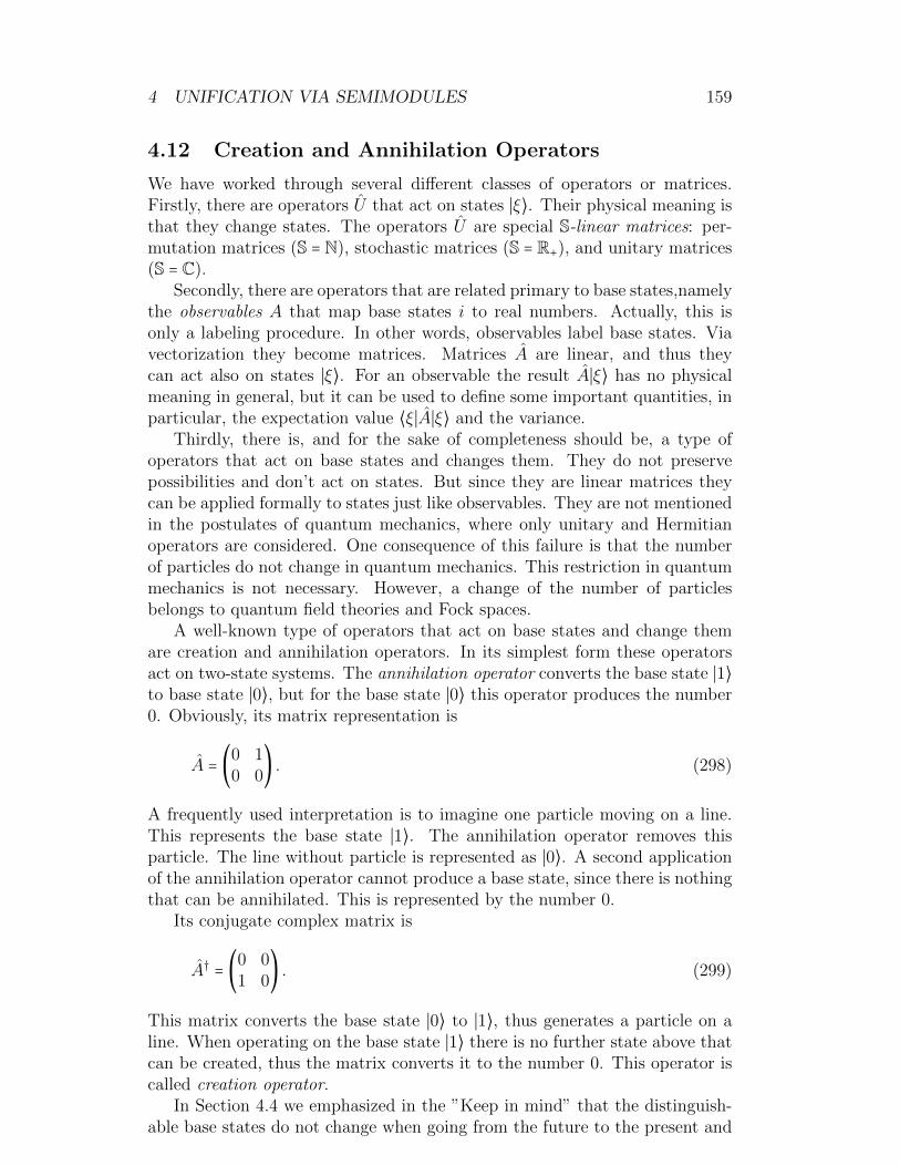
4 UNIFICATION VIA SEMIMODULES 159

4.12 Creation and Annihilation Operators

We have worked through several different classes of operators or matrices.Firstly, there are operators U that act on states ∣ξ⟩. Their physical meaning isthat they change states. The operators U are special S-linear matrices: per-mutation matrices (S = N), stochastic matrices (S = R+), and unitary matrices(S = C).

Secondly, there are operators that are related primary to base states,namelythe observables A that map base states i to real numbers. Actually, this isonly a labeling procedure. In other words, observables label base states. Viavectorization they become matrices. Matrices A are linear, and thus theycan act also on states ∣ξ⟩. For an observable the result A∣ξ⟩ has no physicalmeaning in general, but it can be used to define some important quantities, inparticular, the expectation value ⟨ξ∣A∣ξ⟩ and the variance.

Thirdly, there is, and for the sake of completeness should be, a type ofoperators that act on base states and changes them. They do not preservepossibilities and don’t act on states. But since they are linear matrices theycan be applied formally to states just like observables. They are not mentionedin the postulates of quantum mechanics, where only unitary and Hermitianoperators are considered. One consequence of this failure is that the numberof particles do not change in quantum mechanics. This restriction in quantummechanics is not necessary. However, a change of the number of particlesbelongs to quantum field theories and Fock spaces.

A well-known type of operators that act on base states and change themare creation and annihilation operators. In its simplest form these operatorsact on two-state systems. The annihilation operator converts the base state ∣1⟩to base state ∣0⟩, but for the base state ∣0⟩ this operator produces the number0. Obviously, its matrix representation is

A = (0 10 0

) . (298)

A frequently used interpretation is to imagine one particle moving on a line.This represents the base state ∣1⟩. The annihilation operator removes thisparticle. The line without particle is represented as ∣0⟩. A second applicationof the annihilation operator cannot produce a base state, since there is nothingthat can be annihilated. This is represented by the number 0.

Its conjugate complex matrix is

A† = (0 01 0

) . (299)

This matrix converts the base state ∣0⟩ to ∣1⟩, thus generates a particle on aline. When operating on the base state ∣1⟩ there is no further state above thatcan be created, thus the matrix converts it to the number 0. This operator iscalled creation operator.

In Section 4.4 we emphasized in the ”Keep in mind” that the distinguish-able base states do not change when going from the future to the present and

4 UNIFICATION VIA SEMIMODULES 160

then to the past. They define the facts in the past, the outcomes or elementaryevents in the present, and possibilities in the future.

Keep in mind: The phrase ”one particle moves on a line” de-scribes a fact in the past, an outcome in the present, or a possi-bility in the future. It will become clear whether we talk aboutfuture (quantum mechanics), present (classical probability theory),or past (classical mechanics). Therefore, we do not change a phraselike ”one particle moves on a line” to ”if, in a future action oneparticle would move on a line”, although the latter is correct whentalking about quantum mechanics.

An important aspect is that each 2 × 2-matrix can be constructed withthese two matrices only. If we compose both matrices in series, we obtain theproduct matrices

AA† = (1 00 0

) . (300)

and

A†A = (0 00 1

) . (301)

When multiplying these four matrices with scalars and adding them, then weobtain every 2×2-matrix. Via the tensor product we obtain all important gatesof quantum computing. For example, the controlled-NOT can be written as

⎛⎜⎜⎜⎝

1 0 0 00 1 0 00 0 0 10 0 1 0

⎞⎟⎟⎟⎠= A†A⊗ (B + B†) + (AA† ⊗ 1), (302)

where B and B† are the annihilation and creation operators for the second bit.Feynman601982 was the first who considered how computers can be built usingthe laws of quantum theory. He started to build up all gates using creationand annihilation operators. Notice that these operators are neither unitarynor observables.

In quantum physics these operators are used in many-particle physics andquantum field theories. Please look in those books for an extensive discussionof this subject. See also Section 5.

Keep in mind: In physics there are three important types ofoperators: operators that transform states (permutation matrices,stochastic and unitary matrices), operators that label base states(observables, Hermitian operators), and operators that change basestates (creation and annihilation operators).

60Feynman [1982], Feynman [1986]

4 UNIFICATION VIA SEMIMODULES 161

Finally, we want to mention that there is a set of matrices that belong to allthree classes, namely the Pauli matrices, which we have introduced in Section4.11. Simple computations show:

• The Pauli matrices are unitary, thus transform states.

• The Pauli matrices are Hermitian, thus they are observables.

• The Pauli matrices transform base states, since they are unitary.

4 UNIFICATION VIA SEMIMODULES 162

4.13 Space and Entanglement

It is often mentioned in the literature that there are two fundamental problemswith quantum theory, namely the meaning of superposition and entangle-ment.

We have explained superposition by experimental set-up’s like the slit ex-periments. In order to avoid paradoxes we have formulated quantum mechanicsas a theory describing the future in terms of ”as well as” possibilities. The fu-ture is timeless, there is no ” future clock”. Actually, in the future happensnothing. Perhaps, future might be best described by the phrase ” What couldhappen, when nothing happens? ”

Future itself is timeless, of course. But are there hints that quantum theoryis timeless such that we can classify quantum theory as the theory describingthe future? Yes, the well-known Wheeler-de Witt equation describes quantummechanics without any time-dependence. This equation has generated muchcontroversy, but is out of the scope of these notes. Nevertheless, when wedescribe physics in terms of our trinity ”future-present-past” we must provethat the fundamental equations of physics, in particular those of gravitationand electromagnetism, must be fulfilled, at least approximately.

Indeed, if quantum mechanics is timeless, that is the theory has no externaltime t, then we run into big problems. Spacetime vanishes, and quantummechanics and the theory of relativity can hardly work together. Relativisticquantum mechanics and quantum field theories should be impossible. TheLorentz transformation and its invariant quantities seem to vanish. But couldthere be any other space and an appropriate theory that can replace the four-dimensional spacetime and the theory of relativity?

Related to these questions is the problem of entanglement. There are easyunderstandable forms of entanglement, for instance, two welded coins or whenthe cat is entangled with a box. It is, however, far from being simple whentwo photons are entangled although they are separated by a large distance.Einstein referred to it with the phrase ”spooky action at a distance”. Distance,however, is a property of the underlying space. Could it be that changing thespace leads to a better understanding of this phenomenon?

When we change the underlying space and additionally avoid time t, thenit seems to be not possible to recover our fundamental equations. Let ussummarize some well-known facts about spaces used in physics61.

• Physicists love symmetry. But just when starting with the fundamentalconcept of space, the non-symmetric (3+1)-spacetime with three spatialcoordinates and one time coordinate is used. An alternative is to startwith the (3+3)-phase space. If we don’t involve mass, then the phase

61 Our notation when using coordinates should be mentioned. The Newtonian equationof motion is a second order differential equation usually formulated in Cartesian coordinatesx,v and p. This equation is not invariant for transformations to other coordinate systems likecylindrical or polar coordinates. A big advantage of Hamilton’s equations is their invariancewhen transforming coordinate systems. Then we speak of generalized coordinates, namelygeneralized position q and generalized momentum p. In these notes this distinction does notmatter, and we will use both notation for the coordinates.

4 UNIFICATION VIA SEMIMODULES 163

space consists of symmetric pairs (x, v) ∈ X × V in a position-velocityspace, where X denotes a set of points and V denotes a set of velocities.The set of points allow to define arrows in V with starting and terminalpoints. Vice versa the arrows depict to points. Without points no arrows,and conversely without arrows no points. Positions and their changerequire velocities, and velocities generate starting and terminal points.This remembers at Esher’s ”drawing hands”, where out of a sheet ofpaper two hands, seemingly paradoxical, draw one another into existence.The hands are both, the object and the machine of creation. Neitherhand seems to have an origin, a beautiful symmetry of (3+3)-space.

• The ”drawing hands” and their symmetry is in some sense reflected inthe Hamilton equations

pk = −∂H

∂xk, xk =

∂H

∂pk, (303)

the fundamental equations of classical mechanics. These equations havesix independent variables, three position variables x and three momen-tum variables p. The interpretation in physics is: given any Hamiltonfunction H(x, q) and the values of the position and momenta coordinatesat some time, the equations (303) give the coordinates of the resultingpath at an infinitesimal time later. The complete trajectory in the phasespace is obtained by successively updating the coordinates.

This is the usual interpretation of Hamilton’s equations. But in our in-terpretation these equations describe facts of the past, and we know thatthe past is timeless. What means t? Well it’s just a geometrical parame-ter that allows to describe the solution of the equations in explicit form.The solution is a geometrical object, an ellipse or a more complicatedcurve. Hamilton’s equation are part of the deterministic past.

• The phase space has dimension (3+3). Are there other spaces withthis dimension? Yes, of course. The fundamental theory of electro-magnetism has the same dimension. Maxwell’s equations work with athree-dimensional electric field E and a three-dimensional magnetic fieldB.

• But what does this mean for the theory of general relativity? Does thistheory vanish? At least not completely. Einstein’s field equations de-scribe how matter and radiation determine the curvature of spacetime,and vice versa. These equations are nonlinear. But it is fascinating thatthe linearized field equations turned out to be of the type of Maxwell’sequations in a 3 + 3-space. Moreover, all of the experimental results likethe deflection of light, the gravitational time dilation, the gravitationalradiation, or the correction formula for GPS, emerge in the linear ap-proximation, see for example Ohanian62. In addition, since Maxwell’sequations can easily be quantized (see Section 5.12), the linearized field

62Ohanian [1994]

4 UNIFICATION VIA SEMIMODULES 164

equations of Einstein can easily be quantized. In this sense gravitationcan be easily quantized. Hence, our most fundamental theories can bedescribed in a (3+3)-space.

• But what about Heisenberg’s uncertainty principles, when we changespacetime and use a (3+3)-space? These principles are known to as-sert a fundamental limit to the precision we can know about certainpairs of complementary variables, like position and momentum or timeand energy. The position-momentum uncertainty is in accordance withthe (3+3)-space. There exists, however, no position-time uncertainty ormomentum-energy uncertainty. Uncertainty principles don’t like non-symmetric (3+1)-spaces. They prefer a symmetric dimension.

• Keep in mind: The (3+3)-position-velocity space X ×V is distin-guished by a wonderful symmetry which reminds of Esher’s ”draw-ing hands”. Moreover, the ”spooky action at a distance” of twoentangled photons in (3+1)-spacetime vanishes. The two photonsare welded in the velocity space V . In other words, they can beconnected via a velocity v ∈ V . Notice that the notion of distancedepends on the space.

We have found some basic arguments that support a (3+3)-position-velocityspace. In particular, the fundamental physical theories such as classical me-chanics, gravitation and electromagnetism can be formulated using dimension(3+3). Of great advantage is that this space allows to use our preferred lan-guage of machines.

Remember that we looked at birefringent plates as machines. They arecharacterized by a polarization axis, and by two possibilities, namely theirtwo polarization directions. In the same way we define a position machine.This machine is characterized by a velocity v ∈ V , and by the set X thatrepresent all possible positions. The difference to the calcite is that the angleof polarization is replaced by the velocity, and that we have now a large numberof possibilities, namely all positions.

Think of a position machine as a ”train” moving at constant speed. Don’tthink that this machine is merely a reference frame. This would be true in(3+1)-spacetime. Contrary, this is a real existing machine which is consistentwith our experience. If you are inside a train moving at constant speed andyou toss a ball into the air, then the ball will go straight up and then comesstraight down. The ball has the same inertia as the train. Much more beautifulexamples are provided by astronauts in a gravitational free space. This inter-pretation of trains in a position-velocity space explains the famous riddle ofinertia. Compare the comments in Section 1. Recognize that this explanationdoes not hold valid in the (3+1)-spacetime, thus giving one more argument forthe position-velocity space.

The whole space X × V consists of many position machines. As in thecase of polarization of light, where only the difference between the angles of

4 UNIFICATION VIA SEMIMODULES 165

two polarization axes is relevant, symmetry requires that only the differencebetween the velocities of two position machines is useful. Frequently, we denoteby (X,0) one machine and by (X ′, v) the other machine, where v denotes thisdifference.

The positions in X represent the base states, that is, all possible positionsthat may be occupied in a future experiment. Now we can apply our math-ematical formalism developed above. The number representation is given bythe numbers x ∈X. Asking binary questions in which half a point is, we obtainthe register representation of positions. Finally, vectorization leads to the basestates ∣x⟩.

The states of a position machine are superpositions

∣ξ⟩ =∑x

ξx∣x⟩, ξx ∈ S, ∑x

∣ξx∣2 = 1, (304)

which are classical, random, or quantum depending on whether S = N,S = R+,or S = C, respectively. Using our unified definition of observables, we arrive ina natural and simple manner to observables described as Hermitian operators.

In quantum mechanics the transition from classical observable values toHermitian operators is usually postulated. Here, it turns out to be a con-sequence of carefully distinguishing between states and base states and oursimple process of vectorization.

The (3+3)-position-velocity space contains also velocity machines or ”dualtrains”. This machine is characterized by a distance x ∈ X, and by the setV representing all possible velocities. Given two velocity machines we denoteby (0, V ) one machine and by (x,V ′) the other machine, where x denotes thedistance between both.

We have visualized the concept of ”trains” (X ′, v) and ”dual trains” (x,V ′)in Figure 73. One might imagine motion of physical objects as a change from(x, v) to (x + ∆x, v + ∆v) between trains and dual trains. Since quantumtheory is probabilistic this change must be probabilistic one, and must be inagreement with Feynman’s rules.

Keep in mind: There are good arguments to describe physicalprocesses on the basis of a 3+3-space. In particular, this space canbe viewed as composed of position and velocity machines.

4 UNIFICATION VIA SEMIMODULES 166

'

&

$

%

(x,V´)

v

(0,V)

(0,0) (X,0)

(x,v)(X´,v)

x

Figure 73: The (3 + 3) position-velocity space (X,V ) can be viewed as acollection of machines: the trains (X ′, v) and the dual trains (x,V ′). Theseare displayed for one position and one velocity coordinate. In this space ina future experiment a particle can change from (0,0) to (x, v). Feynman’s(never violated) rules are applied to obtain the related probabilities.

4.14 Clocks and the Lorentz Transform

Above we have given several arguments to replace the (3+1)-spacetime bya (3+3)-position-velocity space. A major reason was that we view quantummechanics as a theory describing the future, and the future is timeless. But ifthere is no spacetime, then there is no theory of relativity. Nevertheless, weask whether we can reproduce the mathematical formalism of special relativity.In particular, we are interested in the key of this theory, namely the Lorentztransform. A second question is: From which principles can we derive theframework of relativity?

Let us consider what is possibly the deepest of all philosophical puzzles,namely the nature of time. Clocks are used to compare the speed of differentobjects, say a group of runners on a certain distance. When looking at his clockeach runner observes a value, called the time for the given distance. Insteadof runners, let us look at two trains (X,0) and (X ′, v), or position machinesif you like, see Figure 74. Each train is equipped with a clock at places 0 ∈ Xand 0′ ∈X ′. Both trains differ with respect to the relative velocity v. How canwe measure the velocity v.

We assume that at the beginning both clocks are synchronized, that is,the positions 0 and 0′ as well as the clockhands are coincident. The lengthxclock > 0 denotes the distance traveled by the tip of the clockhand in one round,and ∣vclock∣ denotes the clockhand’s constant magnitude of velocity. Hence, theratio xclock/∣vclock∣ characterizes the clock itself, and we can choose the clockunit as

xclock∣vclock∣

= 1 [sec = meter/mps], (305)

4 UNIFICATION VIA SEMIMODULES 167

'

&

$

%

v

v

vclock

vclock

x

(0´,v)

(0,0)

(X´,v)

(X,0)

Figure 74: Two trains (X,0) and (X ′, v). Both trains are equipped with aclock at (0,0) and (0′, v). At the beginning, we assume that both places,0 and 0′, and the position of the clockhands coincide. Then the clocks aresynchronized.

where we have defined the time-independent velocity unit as mps, a shortcut formeter per second. Notice that now time is a derived quantity in the position-velocity space.

Let us assume that the second train has covered the distance x in X.Moreover, we assume that the tip of the clockhand of the first clock has covereda distance xc. After 1 round the clockhand has covered the distance xc = xclock.After 2 rounds the clockhand has covered the distance xc = 2xclock. After 2.5rounds the clockhand has covered the distance xc = 2.5xclock, and so on. Hence,it is natural to define the time t of the first clock via the number of roundscovered by the clockhand:

t = xcxclock

. (306)

The parameter t denotes the clock’s measurable or observable value whichdefines a quantity called time, derived in X × V . Now t is not an externalfundamental parameter, but a parameter that is related to a unique specificclock.

We assume uniform motion, that is, the position-independent quantity vis constant. Then the ratio of the distances must be equal to the ratio of thevelocities, that is,

x

xc= v

∣vclock∣. (307)

Then

x = v xc∣vclock∣

= v xcxclock

xclock∣vclock∣

, (308)

4 UNIFICATION VIA SEMIMODULES 168

From these formulas we obtain the fundamental kinematic equation

x = vt, (309)

where time t is the derived value for the first clock in our (3+3)-space, de-pending on distance and velocity only. This coincides with Einstein’s advice:

Time is what clocks measure.

But in contrast to Einstein we do not postulate the (3+1)-spacetime, and donot assume a maximal speed of light.

There are various clocks like pendulum clocks, spring-driven clocks, quartzclocks where a quartz crystal vibrates, and atomic clocks based on the vibrationof electrons in atoms. Clocks are physical systems that change positions andvelocities. They are machines inside our universe, and thus can be describedas observables, that is, matrices.

In most cases clocks perform periodic processes of motion, which occuragain and again in the same way, for example, the reciprocation of a pendulum.We assume that they always take approximately the same period, so that theycan provide us with a uniform time standard. The clock can be described asa machine in position-velocity space such that the observed time t = t(x, v)depends on position and velocity.

Let (X, t) and (X ′, t′) denote the coordinates of trains and times of the firstand second clock, respectively. Neither clock is preferred. From the reversalpoint of view, the first clock ist uniformly moving with velocity −v with respectto the second clock. Hence, we obtain as before the fundamental kinematicequation

x′ = −v t′. (310)

It is always possible to transform between the coordinates of both trains.The question is whether there exists a non-singular linear transformation. Letus make the Ansatz that there is a linear transformation

( x′

t′) = Λ ( x

t) = ( Λ11 Λ12

Λ21 Λ22)( x

t) . (311)

This is the most simple model. Obviously, the matrix Λ = Λ(v) depends onthe scale v ≠ 0. Moreover, we can assume that the covered distance x, andthus the time t of the first clock, are non-zero.

This equation must hold true for all possible coordinates. If we set x′ = 0,then the first line of this equation implies Λ11 ≠ 0, since otherwise Λ12 must bezero, yielding a singular transformation matrix. Dividing the first equation byΛ11 gives

−Λ12

Λ11

= xt= v. (312)

Hence, Λ12 = −Λ11 ⋅ v and (311) implies

x′ = Λ11 ⋅ (x − vt). (313)

4 UNIFICATION VIA SEMIMODULES 169

Since x′ = −v ⋅ t′, the equations (311) and (313) yield

t′ = −1

vx′ = −Λ11

vx +Λ11t = Λ21x +Λ22t. (314)

Hence, Λ11 = Λ22 and

t′ = Λ22 (Λ21

Λ22

x + t) . (315)

Let us switch to the more appropriate notation

γ = γ(v) = Λ11 = Λ22 and β = β(v) = Λ21/Λ22. (316)

Then the equations (313) and (315) can be written as

x′ = γ(x − vt), t′ = γ(βx + t), (317)

yielding the transformation matrix

Λ = γ ( 1 −vβ 1

) . (318)

This is almost the Lorentz transformation. We have only to determine theconstants β and γ.

Let us look at three trains. If we can transform coordinates between (X, t)and (X ′, t′) with respect to velocity v, then we can transform coordinatesbetween (X ′, t′) and (X ′′, t′′) with respect to a velocity u. Of course, we cantransform coordinates between (X ′′, t′′) and (X, t) by consecutive composition.In matrix form it follows that

( x′

t′) = γ(v)( 1 −v

β(v) 1)( x

t) , ( x′′

t′′) = γ(u)( 1 −u

β(u) 1)( x′

t′) ,

(319)

and

( x′′

t′′) = γ(v)γ(u)( 1 − β(u)v −u − v

β(v) + β(u) 1 − β(v)u )( xt

) . (320)

Since the transformation matrix must be of type (318), the diagonal elementsare equal to one, yielding for every u and v:

1 − β(u)v = 1 − β(v)u, or equivalentlyu

β(u)= v

β(v). (321)

Clearly, the ratio v/β(v) = % must be a nonzero constant. In other words,it is invariant for any scale v ≠ 0, and therefore

Λ(v) = γ(v)( 1 −vv/% 1

) . (322)

4 UNIFICATION VIA SEMIMODULES 170

Now we can transform from (X ′, t′) to (X, t), and then backwards yielding

( x′

t′) = γ(v)( 1 −v

v/% 1)( x

t) , ( x

t) = γ(−v)( 1 v

−v/% 1)( x′

t′) , (323)

and

( xt

) = γ(−v)γ(v)( 1 v−v/% 1

)( 1 −vv/% 1

)( xt

)

= γ(−v)γ(v)( 1 + v2/% 00 1 + v2/% )( x

t) .

(324)

This equation must hold for every x and t, and we obtain

γ(−v)γ(v) ⋅ (1 + v2

%) = 1. (325)

Since both systems (X, t) and (X ′, t′) are on an equal footing, and x′ = γ(v)(x−vt) translates symmetrical to x = γ(−v)(x′ − (−v)t′), the nonzero value γ(v)does not depend on the direction of v. Therefore, γ(v) = γ(−v) implying

γ(v)2(1 + v2

%) = 1. (326)

Taking the square root and substituting into equation (314), we get the well-known two-dimensional Lorentz transformation

x′ = γ(x − vt), t′ = γ(v%⋅ x + t), γ(v) = ±1/

√1 + v

2

%. (327)

A simple computation shows the invariant quantity

−%(t′)2 − (x′)2 = −%t2 − (x)2. (328)

The fundamental constant % is nonzero, and thus can be positive or negative.Since γ is dimensionless, % has the units of a squared velocity. Firstly, let usconsider the case % < 0, and let c = √−%. Then

γ(v) = ±1/√

1 − v2

c2, (329)

and the invariant (328) takes the form

(ct′)2 − (x′)2 = (ct)2 − (x)2. (330)

This is the famous Minkowsky distance which is invariant with respect toLorentz transformations. Therefore, every relative speed distance ∣v∣ betweentwo clocks has to satisfy the condition ∣v∣2 < c2, and thus must be smaller thanc; otherwise γ would be imaginary, illicitly.

4 UNIFICATION VIA SEMIMODULES 171

In physics the constant c is identified with the maximal speed of light.Hence, the maximal speed of light is a strictly upper bound for relative velocitydistances between clocks. The identity

x = vt = κ(ct) = κx0, 0 < κ = v/c < 1 (331)

shows that we have obtained for all clocks a common length ruler x0 = ct.Obviously, the clocks differ in their characteristic ratios. All clocks have thesame ruler ct, and the invariant (328) has the value (ct)2(1 − κ2).

At the beginning the coordinates of the relative velocity v could have un-substantially numerical values, and in some sense there was some arbitrarinesswhen choosing x = vt. In other words the labeling was not reasonable. Butnow we have a bounded characteristic number κ for each train, and the com-mon ruler ct for all trains. Summarizing, we have obtained physical reasonablecoordinates in the form of state-coordinates and the same scale in all possibleposition machines.

Additionally, in this case we get a nice interpretation. Since % = (ic)2,formula (328) implies the invariant

(x)2 + (ict)2 = x′2 + (ict′)2 = c2t2. (332)

Hence, for negative %, Lorentz transformations can be viewed as rotationsabout the origin with a real position coordinate x and an imaginary coordinate,the imaginary velocity ic. This suggest a position-velocity space X × iV withimaginary velocities.

Finally, let us consider the case % > 0, and let c = √%. Then the transfor-

mation describes simply an orthogonal rotation of the coordinates (ct, x). Thecoordinates of v cannot be further specified, the set of possible values κ is un-bounded, and the equation (328) makes not much sense, because we have thesame arbitrariness as before. Therefore, this case is physically uninteresting.

Keep in mind: The position-velocity space allows to define clocksas machines that provide a derived quantity, the time. A few simplearguments yield the mathematical framework of special relativity.This derivation does not require the usual postulates of special rela-tivity, namely that (i) the laws of physics are the same in all inertialframes of reference, and that (ii) the speed of light in free space hasthe same value c in all inertial frames of reference.

In summary, the position-velocity space allows to describe Hamilton’s clas-sical mechanics, the theory of special relativity, and a reasonable explanationof entanglement. To emphasize the central difference, we remember what Her-man Minkowski wrote:

Henceforth, space by itself, and time by itself, are doomed to fadeaway into mere shadows, and only a kind of union of the two willpreserve an independent reality. (80th Assembly of German Natu-ral Scientists and Physcists at Cologne 1908)

4 UNIFICATION VIA SEMIMODULES 172

Our approach is rather radical when viewing t as a variable depending on(x, v), and describing reality as a kind of union of position and velocity. Thederived parameter t has no relation to motion and should be not mixed upwith the time that is used in physics for describing the dynamics.

In almost all books about relativity the word observer is in use. Observingis based on human beings. But the laws of physics should not depend onthe existence of human beings, whatever they are. Only physical objects ofreality can exist. Mathematical entities such as frames of reference do notexist in reality, and in no manner they can move. We arrived at the Lorentztransformation via machines, called clocks, in the position-velocity space. Thefact, however, that the times t and t′ differ seems to be strange. It comes outsolely of simple transformations, but the mathematics explains nothing. Whydiffer these times? Let us look at an example in the one-dimensional positionspace. Assume you have a pencil, and the pencil point is 1 meter away fromyour eye. You have measured this with a tape measure. What does this valuemean? Actually nothing. Another person, a so called observer, measuring fromanother position obtains another value. Each value is possible. The observersdisagree. But there is another important quantity, the length of the pencil,that is, the difference between the pencil tip and its end. Independent of theposition, all observers measure the same length. The length is independent ofthe observer. That is the key to special relativity. Clocks can provide differentvalues. This is not surprising, and these values are unimportant. Importantare the values that are invariant with respect to the Lorentz transform, suchas the distance (330). The well-known Hafele-Keating experiment has showndifferent times between clocks that are moving with different velocities. In thefour-dimensional spacetime this experimental result is surprising and perhapsweird, since velocity is a derived quantity. In a position-velocity space thevelocity is an independent quantity leading to reasonable results.

Keep in mind: We have seen that the mathematical frameworkof quantum mechanics applies also to large objects. Now we haveseen that the theory of relativity can be derived from simple trans-formation rules that are necessary from a mathematical point ofview. It is not necessary, however, to postulate the existence oflight itself or a maximal speed of light.Time dilation and length contraction are not strange, they are sim-ple consequences of our viewpoint that clocks are derived machinesin a position- velocity space without external time parameter.

4 UNIFICATION VIA SEMIMODULES 173

4.15 Dimension of Space

There are some deep fundamental questions in physics. What can we say aboutthe dimension of physical reality? Why is the underlying space in most physicalmodels the (3+1)-dimensional spacetime? Are there more useful spaces withother dimensions? Can mathematics perhaps dictate dimensions?

Unfortunately, we can only describe superficially whether and how thesefundamental questions might be answered. It requires knowledge about thedifficult theory of Lie groups and Lie algebras, which we cannot treat exten-sively within the context of these lecture notes. However, a rough introductionis presented in the Appendix 7. Hopefully, it might help to understand theessential aspects.

There are several physical theories that are based on various dimensions.For example, we have considered a (3+3)-dimensional position-velocity space,and we defined therein a dependent variable time. This time is what a clockmeasures. The Kaluza-Klein theory is a field theory that unifies gravitation andelectromagnetism in a 5-dimensional space which is beyond the usual (3+1)-dimensional spacetime. String theories require extra dimensions of space. Inbosonic string theory, the space is 26-dimensional, in superstring theory it is 10-dimensional, and in M-theory it is 11-dimensional. Quantum chromodynamics,the theory of strong interactions between quarks and gluons, is a quantum fieldtheory that is based on the 3-dimensional complex space. At a first glance eachdimension might be useful, say 37, 543, or any other number.

What is a reason why the previous questions about the dimensions areimportant and even fundamental? There is an old well-known story. Duringa meeting in the year 1953 Fermi criticized a model developed by Dyson. Hequoted John von Neumann who said:

With four parameters I can fit an elephant, and with five I canmake him wiggle his trunk.

He pointed out that nobody should be impressed when complicated, high-dimensional models fit all data sets. With enough parameters, you can fitanything. Obviously, the same argument applies also to the number of vari-ables in a physical theory defining its dimension; a fixed value of a variable isa parameter. Hence, a major goal is to develop useful physical theories withlowest possible dimensions and with few parameters. It is amusing that Mayeret al.63 gave a five parameter model that encodes the elephant including itswiggling trunk, see Figure 75.

When thinking about spaces, we can imagine the most diverse geometries:non-smooth geometries, twisted geometries like a pretzel, and many others. Ofcourse, without any reasonable assumptions we cannot answer our questionsabove. It seems to be natural, however, to assume that in a plausible spacewith reasonable geometry we can define simple geometric objects, as is possiblein an inner-product space like Rn or Cm. In these inner-product spaces we candefine normal vectors, planes, rotations, unitary operators, and we have a greatunderstanding and experience with such spaces.

63Mayer, Khairy, Howart [2010]

4 UNIFICATION VIA SEMIMODULES 174

'

&

$

%

50 – 30i 18 8i

40 20i

12 – 10i

14 – 60iFigure 75: Three snapshots of the wiggling trunk with the five complex pa-rameters that encode the elephant.

4 UNIFICATION VIA SEMIMODULES 175

In Section 4.11 we have developed the quantum mechanics of two-statesystems in terms of real rotations acting on real three-dimensional vectors,and on unitary matrices acting on two-dimensional complex vectors. Actually,we have seen that for each real rotation there must correspond a unitary matrixand vice versa. Consequently, both spaces, the three-dimensional real spaceR3 and the two-dimensional complex space C2, are compatible in this sense;not R4 and C2 as one would expect since each complex number is describedby two real numbers.

This example is so simple and fundamental that it should apply to allreasonable spaces that are used in physics. Hence, the physical space can bethought of in two different ways. There is the real space that allows to rotatereal vectors, and then there is the complex space where unitary matrices acton complex vectors. We accept only spaces that are compatible in this sense.Hence we try to answer the following question: For which pairs (m,n) is then-dimensional real space Rn compatible with some m-dimensional complexspace Cm with respect to rotations?

In other words, for given pairs (m,n) we ask whether there is a uniquecorrespondence between real n-dimensional rotations and complex unitary m-dimensional operators. All other dimensions (m,n) that don’t satisfy thisbasic, simple and reasonable requirement would be ruled out. We call this re-quirement the space-compatibility postulate. Notice that spin and polarizationsatisfy this postulate, since two state-systems can be described in terms of thereal space R3 and the complex space C2.

But if we consider only the spaces Rn and Cm, then we would rule outthe (3+1)-dimensional spacetime, since the spacetime inner product is not thesame as in the four-dimensional real Euclidean space R4. In Section 4.6 wehave defined the inner product (221) of two vectors. In the theory of relativitythe concept of pseudo-Euclidean spaces is used. In the following we allow alsopseudo-Euclidean spaces in our considerations.

Let p, q be two integers with p+q = n. Then the pseudo-inner product of twovectors ∣φ⟩, ∣ψ⟩ ∈ Cn is defined as the sum of the first p terms φ∗i ψi, i = 1, . . . , pminus the sum of the remaining q terms φ∗jψj, j = p + 1, . . . , n, that is,

⟨φ∣ψ⟩ = φ∗1ψ1 + . . . φ∗pψp − φ∗p+1ψp+1 − . . . − φ∗nψn. (333)

We denote the complex space equipped with an pseudo-inner product by Cp,q,and the real space equipped with an pseudo-inner product by Rp,q.

In our geometrical example where a ball is placed on a spherical surfacewe have considered real rotations and unitary transformations. Both leavethe inner product invariant, namely the length of the real normal vectors andthe areas of the spherical surface. Such transformations are called symmetryoperations.

Now comes our central question. Which pairs of real and complex groupsare compatible and admit a unique correspondence, at least between theirinfinitesimal rotations?

This is an old classical question which has long ago been answered byBarut and Raczka64 1965. They provide a table of all possible compatible

64Barut et al. [1965]

4 UNIFICATION VIA SEMIMODULES 176

correspondences. We have displayed these correspondences in Table 5. This

Table 4: Compatible groups and spaces

Real compatible Complexso(2) ≅ u(1)so(1,2) ≅ su(1,1)so(3) ≅ su(2)so(1,3) ≅ sl(2,C)so(4) ≅ su(2)⊗ su(2)so(2,4) ≅ su(2,2)so(6) ≅ su(4)

is in fact a very surprising result. Normally, one would expect that a compatiblecomplex space exists for every real space. This is obviously not the case. Only7 pairs exist.

The numbers in both columns denote the dimensions of the underlyingspaces, and the symbols ”so” or ”su’ denote the infinitesimal rotations onthese spaces. For example, so(2), so(1,3), and su(2) denote the infinitesi-mal real rotations of the Euclidean space R2 with determinant equal one, theinfinitesimal rotations on the pseudo-Euclidean space R1,3 with determinantequal one, and the infinitesimal unitary rotations on the complex space C2 withdeterminant equal one, respectively. The basic definitions as well as the ideaof the proof are sketched in appendix 7. Readers without any knowledge of Lietheory should read this appendix first. With capital letters SO(2), SO(1,3),and SU(2) we denote the corresponding groups.

The next surprising observation is that the Kaluza-Klein theory, all stringtheories, and quantum chromodynamics are ruled out; the real space dimen-sions n = 5,10,11,26 and the complex space dimension m = 3 do not occur.The Standard Model of particle physics, a gauge quantum field theory con-taining the internal symmetries of the product group SU(3) ⊗ SU(2) ⊗ U(1)does not fit into this table. All these theories do not satisfy our compatibilitypostulate. Hence, the simple example, where we derived everything importantabout two-state systems such as spin and polarization, does not work in thesetheories. Hence, the simple question ”on which side of a plane a ball may bepositioned on a spherical surface” cannot not be discussed there. But manyphysicists, like von Weizsacker with his Ur-theory, think that physical realitycan be built up with two-state systems. Remember that two-state systems arethe basic building blocks in quantum information theory.

Let us now look more precisely on Table 4. The first compatible paircontains the simplest complex group U(1). Geometrically, it describes therotational symmetry of a circle using complex (1×1)-matrices. This symmetryis well-known as the symmetry group for electromagnetic interactions.

The second pair is rarely used in physics. However, there are some relationswith symplectic algebra and canonical transformations. In the paper of Marcel

4 UNIFICATION VIA SEMIMODULES 177

Novaes65 a nice application is presented how to obtain the energy spectrum ofthe hydrogen without solving the Schrodinger equation.

The third pair shows the compatibility of the three-dimensional real Eu-clidean space with the two-dimensional complex space. This relationship hasvarious applications, among them the three-dimensional spaces of position andvelocity, or electric and magnetic fields. Polarization and spin can be describedwith two-dimensional complex vectors. The group SU(2) is also known tomodel weak nuclear interactions.

The fourth pair is well-known. It contains the widely used (3+1)-dimensionalspacetime. It satisfies our space-compatibility postulate. But the pseudo-orthogonal Lorentz rotations are related to two-dimensional complex matricesthat are not necessarily unitary. Thus they do not preserve the inner product.With regard to our example, this has the consequence that the total area ofthe spherical surface is not preserved. This fact is another disadvantage in ad-dition to the asymmetry of spacetime. Moreover, it is a non-Euclidean space.These arguments may be hints that the spacetime is helpful, but seeminglynot the fundamental space of a physical theory. Consequently, quantum fieldtheories that are based on spacetime would be ruled out, although they mightbe useful in many situations.

The fifth pair is very promising. The space is Euclidean. The group ofreal four-dimensional rotations SO(4) contains the group of all real three-dimensional rotations which is compatible with the group SU(2) of complextwo-dimensional rotations as shown above. This shows the close relationshipbetween the groups SO(4), SO(3)⊗SO(3), and SU(2)⊗SU(2). Both lattergroups imply dual (complementary) variables that lead naturally to Heisen-berg’s uncertainty relations. Moreover, they explain why in electromagnetismwe have an electric field and a magnetic field. The same applies to positionand velocity or momentum. Finally, the corresponding space explains entan-glement and thus avoids distant spooky effects. All these properties coincideswith our observations in Section 4.13.

The sixth pair is substantial in twistor theory which is out of scope of thislecture notes.

The last pair is perhaps the most promising space. The group of real six-dimensional rotations SO(6) contains SO(4) as a subgroup, and thus containsall its nice properties. Moreover, it is a well-understood Euclidean space.

Mirman investigated in a series of papers how symmetry principles andgroup theory can be used in order to determine the dimension of space. A nicepresentation, proofs, many references and interesting aspects can be foundin his excellently written book ”Our Almost Impossible Universe: Why theLaws of Nature Make the Existence of Humans Extraordinarily Unlikely”66.He concluded, however, that physics and our universe is only possible in the3 + 1-dimensional spacetime. Using further arguments, with which I do notagree, he ruled out any other dimension.

65Noveas [2004]66Mirman [2001, p. 197]

4 UNIFICATION VIA SEMIMODULES 178

4.16 Teleportation: the Experiment

Zeilinger67 writes in his articles that ”the science-fiction dream of ’beaming’objects from place to place is now reality - at least for particles of light”. More-over, he describes rather detailed his experimental set-up. We have alreadydiscussed teleportation in Section 3.7 with the association that Alice and Bobshare an entangled pair of photons, and Alice wants to send an unknown pho-ton state to Bob who is far far away with his photon. Since it is not possible totransport a specific photon, not surprisingly in the Innsbruck experiment Aliceand Bob or any other observers are absent. Especially, Bob does not carry aphoton. Thus, let us now consider to what extend the described associationwith Alice and Bob is realized in the Innsbruck experimental set-up. Thisexperiment is briefly described in Figure 76.

In this experiment a brief pulse of ultraviolet laser light passes from left tothe right through a beta barium borate crystal BBB and creates an entangledpair of photons ∣AB⟩. Photon ∣A⟩ is reflected at mirror M3 and sent to thesemireflecting mirror SM that serves as a polarizing beam splitter. The otherone ∣B⟩ moves to the calcite crystal and is detected either in D3 or D4. Theremaining part of the pulse is reflected back at mirror M1, passes throughthe crystal once more, and creates a second entangled pair of photons ∣CD⟩.Photon ∣C⟩ interacts with detector D5, and thus certifies that its colleague∣D⟩ is ready for teleportation. Photon ∣D⟩ passes a calcite crystal which hasa certain given polarization axis. In one of both exit beams of the calcite thisphoton comes out with a new polarization state, say ∣ψ⟩. This new preparedstate is known, because the calcite’s polarization axis is known. The interactionof ∣ψ⟩ with ∣A⟩ at the SM implies four possibilities: both photons are reflected,both photons pass, ∣ψ⟩ is reflected and ∣A⟩ passes, and vice versa. It turns out,and we show it below that quantum interference implies that photon state ∣B⟩coincides with state ∣ψ⟩ whenever both detectors D1 and D2 register a photon.Then it is said that teleportation is testified. Subsequently, we describe theessential parts more detailed.

The first experimental task is the creation of entangled pairs of photons.One way to do this is called parametric down-conversion: a laser emits photonsof high frequency ωP and momentum kP , say ultraviolet light, and the photonpasses through a BBB which creates two photons of lower energy, say redones. The two photons of lower energy must satisfy the conservation of energy(ωP = ωA + ωB) and the conservation of momentum (kP = kA + kB). Theseconservation conditions imply that photon pairs are emitted which have nodefinite polarization, but are entangled. Actually, using a second BBB and ahalf wave plate it is possible to create every Bell state. Nowadays, producingentangled pairs of photons is experimentally an easy task.

The second task is to entangle two independent photons, photon 1 in state∣ψ⟩ and photon 2 in state ∣A⟩. This is the most difficult experimental partof teleportation. It uses a polarizing beam splitter SM which, roughly spo-ken, consists of a birefringent material and splits light into beams of differentpolarization.

67?Zeilinger [2000]

4 UNIFICATION VIA SEMIMODULES 179

'

&

$

%

detector D1 detector D2

semireflectingmirror SM

calcitecrystal

mirror M2 mirror M3

calcitecrystal

BBB-crystal D3

D4D5

|ψ

|D |A

|B |C

mirrorM1

laser

Figure 76: In the Innsbruck experiment two short pulses of laser light passfrom left to right through a beta barium borate crystal BBB. Let the pulseproduce the entangled pair of photons ∣AB⟩. Let the second pulse, reflectedback at mirror M1, create a further entangled pair ∣CD⟩ when passing thecrystal. The photon ∣D⟩ is reflected at mirror M2 and passes a calcite thatprepares photon ∣D⟩ in the specific state ∣ψ⟩. If a photon ∣C⟩ is detected indetector D5, it follows that in fact ∣ψ⟩ is sent to the polarizing beam splitterSM that (assuming an idealized experimental set-up) superposes there withphoton ∣A⟩ yielding a Bell state. This superposition destroys ∣ψ⟩. It turns outthat the photon state ∣B⟩ coincides with ∣ψ⟩ provided the detectors D1 and D2have registered two photons. Hence, teleportation is claimed.

4 UNIFICATION VIA SEMIMODULES 180

Let the photon to be teleported have the polarization

∣ψ⟩ = α∣0⟩ + β∣1⟩, (334)

and let

∣AB⟩ = 1√2(∣01⟩ − ∣10⟩) (335)

be the entangled Bell state of the pair of photons ∣A⟩ and ∣B⟩. The currentstate of all three photons is

∣ψAB⟩ = (α∣0⟩ + β∣1⟩)⊗ 1√2(∣01⟩ − ∣10⟩)

= 1√2(α∣001⟩ + β∣101⟩ − α∣010⟩ − β∣110⟩).

(336)

We have already considered the four maximally entangled Bell states

∣φ−≠⟩ = 1√

2(∣10⟩ − ∣01⟩),

∣φ+≠⟩ = 1√

2(∣10⟩ + ∣01⟩),

∣φ−=⟩ = 1√

2(∣00⟩ − ∣11⟩),

∣φ+=⟩ = 1√

2(∣00⟩ + ∣11⟩).

(337)

The first one is antisymmetric, that is, it changes the sign if we change 0 to 1and 1 to 0. The remaining three Bell states are invariant when interchanging0 and 1. Hence, they are symmetric.

Using the coordinate representation of these states, it follows immediatelythat the four Bell states form an orthonormal base in C4. Hence, we canexpress the state ∣ψAB⟩ in terms of the Bell states. A short computationshows

∣ψAB⟩ =

1√2{∣φ−

≠⟩⊗ (−α∣0⟩ − β∣1⟩)

+∣φ+≠⟩⊗ (−α∣0⟩ + β∣1⟩)

+∣φ−=⟩⊗ (α∣1⟩ − β∣0⟩)

+ ∣φ+=⟩⊗ (α∣1⟩ + β∣0⟩)} .

(338)

Notice that this is simply a mathematical manipulation that expresses ∣ψAB⟩with respect to the basis of Bell states; nothing physical has happened.

Therefore, the photons ∣ψ⟩ and ∣A⟩ interact at the polarizing beam splitteryielding one of the four Bell states, instantaneously Bob’s third photon is inone of the four states

∣B⟩ ∈ { (−α∣0⟩ − β∣1⟩), (−α∣0⟩ + β∣1⟩),(α∣1⟩ + β∣0⟩), (α∣1⟩ − β∣0⟩) } , (339)

4 UNIFICATION VIA SEMIMODULES 181

in each case with probability 1/4 according to Born’s rule.There are three possibilities that can happen: both particles are detected

in D1, or both particles are detected in D2, or both detectors register oneparticle. Let us consider the latter case. A deeper analysis shows that inthe case where both detectors register a photon, the third photon ∣B⟩ has theoriginal state ∣ψ⟩. Thus, instantaneous teleportation is claimed.

Actually, the situation is more complicated. Teleportation means that acomplete object is teleported. But the complete object or unity is the entangledpair, not a fragment of the pair. Since we underlay the space X × V , theentangled pairs ∣AB⟩ and ∣CD⟩ are welded in V . Spooky distant effects don’toccur in this space. This entanglement is also expressed in the conservationof energy and momentum. The complete pair ∣CD⟩ is not teleported, only itsfragment ∣D⟩ which changes to ∣ψ⟩ when passing the calcite crystal. Thus, itis doubtful to speak of teleportation. Actually, an interaction between ∣A⟩ and∣ψ⟩ takes place at SM, which can be described as a superposition of the fourBell states. This, of course, must have a related influence on ∣B⟩, due to theentanglement between ∣A⟩ and ∣B⟩.

An important aspect is that the conflict with the theory of relativity hascompletely disappeared, since there are no more distant effects in the position-velocity space. The pair is a unit. The usual arguments about the conflictbetween quantum teleportation and relativity theory, as discussed in Section3.10, vanish.

4 UNIFICATION VIA SEMIMODULES 182

4.17 Uncertainty Principle

Some years ago a doctor in a hospital asked me whether the uncertainty in themedical diagnosis and the medical treatment is a manifestation of Heisenberg’suncertainty principle, that “nothing in nature is precisely defined”. Actually, Isaid “No”. My consideration was that a person consists of about 1028 interac-tion atoms that average to classical values. A person walking one body lengthperforms an action value of about 1036h. From the point of view of medicinehuman beings are best described by average values and probability theory.

Frequently, uncertainty reflects situations that involve imperfect or un-known information. But it arises in several other different ways. For instance,if one observable is measured, or if predictions about future events are re-quired. It appears in many areas of research, including physics, engineering,economics, sociology or information science.

Probability theory is widely used to describe uncertainty, in many casesfor one observable or random variable. But in quantum theory, the famousHeisenberg uncertainty principle makes a statement about two observables.This principle is known to put limits on the accuracy about two complementaryquantities like position and momentum or different spin directions. Histori-cally, Heisenberg (1927) derived the position-momentum uncertainty in twoways. Firstly, by localizing a particle through scattering with high-energyphotons, and secondly by investigating the Fourier relationships of free wavepackets. In both cases he showed that the product of position and momentumuncertainty is of the order of Planck’s constant h. Heisenberg’s notation ofuncertainty cannot be explained just by ignorance, but it is believed by mostphysicists that this principle is a fundamental property of nature. Exemplary,we quote from the beautiful written textbook of Zetteli68 about quantum me-chanics:

On the one hand, the Davisson-Germes and the double-slit ex-periments have shown that microscopic material particles give riseto interference pattern. To account for the interference patterns,we have seen that it is imperative to describe microscopic particlesby means of waves. Waves are not localized in space. As a resultwe have to give up on accuracy to describe microscopic particles,for waves give at best a probabilistic account. .... The classicalconcepts of exact position, exact momentum, and unique path of aparticle therefore make no sense at the microscopic scale. This isthe essence of Heisenberg’s uncertainty principle.

In the following we shall argue that the uncertain principle is not restrictedto microscopic problems, but applies also to macroscopic ones. Moreover, wegive another interpretation which results from looking at quantum mechanicsas a theory of the future. Let us understand what we mean by uncertaintyfrom the mathematical point of view. Given a state

∣ψ⟩ =∑i∈I

ξi∣i⟩, ∑i

∣ξi∣2 = 1, ξi ∈ S (340)

68Zetteli [2009]

4 UNIFICATION VIA SEMIMODULES 183

we derived in Section 4.10 the expectation value of an observable

⟨A⟩ψ = ⟨ψ∣A∣ψ⟩, (341)

and its variance

(∆A)2 = ⟨A2⟩ψ − ⟨A⟩2ψ = ⟨ψ∣(A − ⟨A⟩ψ1)2∣ψ⟩ (342)

the latter also called uncertainty. Since A is Hermitian, equation (342) impliesthe identity

(∆A)2 = ⟨ψ∣(A − ⟨A⟩ψ1)†(A − ⟨A⟩ψ1)∣ψ⟩

= ∥(A − ⟨A⟩ψ1)∣ψ⟩∥2.(343)

Hence, the variance vanishes if and only if

(A − ⟨A⟩ψ1)∣ψ⟩ = 0, (344)

that is, state ∣ψ⟩ must be an eigenvector of A. Equation (245) tells us that ∣ψ⟩must be one of the base states ∣i⟩. We notice that uncertainty of an observableis not present if state ∣ψ⟩ is one of its base states. In classical mechanics S = N,each state is a base state, and there can be no uncertainty.

In classical probability theory and in quantum mechanics the set of basestates and the set of states differ such that uncertainty of a random variable orobservable is present. But this uncertainty has nothing to do with Heisenberg’suncertainty principle in quantum mechanics.

A fundamental question in quantum theory is:

• Under which conditions are two observables A and B certain in conjunc-tion, that is, their variances (∆A)2 and (∆B)2 vanish always simultane-ously?

Equations (343) and (344) tell us that both observables are certain simultane-ously, if and only if they have the same eigenvectors, that is,

A∣i⟩ = Ai∣i⟩ and B∣i⟩ = Bi∣i⟩ (345)

for all base states ∣i⟩ with i ∈ I. In particular, both observables must be definedon the same set of base states. Only their labeling, namely their eigenvalues,can be different. In classical mechanics and classical probability theory wehave seen that there is only one bases, and each number of observables arecertain simultaneously.

In quantum theory, where S = C, this nice property does not hold true,since their exist different bases, as we have seen. Let us look in greater detailat the two observables

C ∶= A − ⟨A⟩ψ1, (346)

and

D ∶= B − ⟨B⟩ψ1. (347)

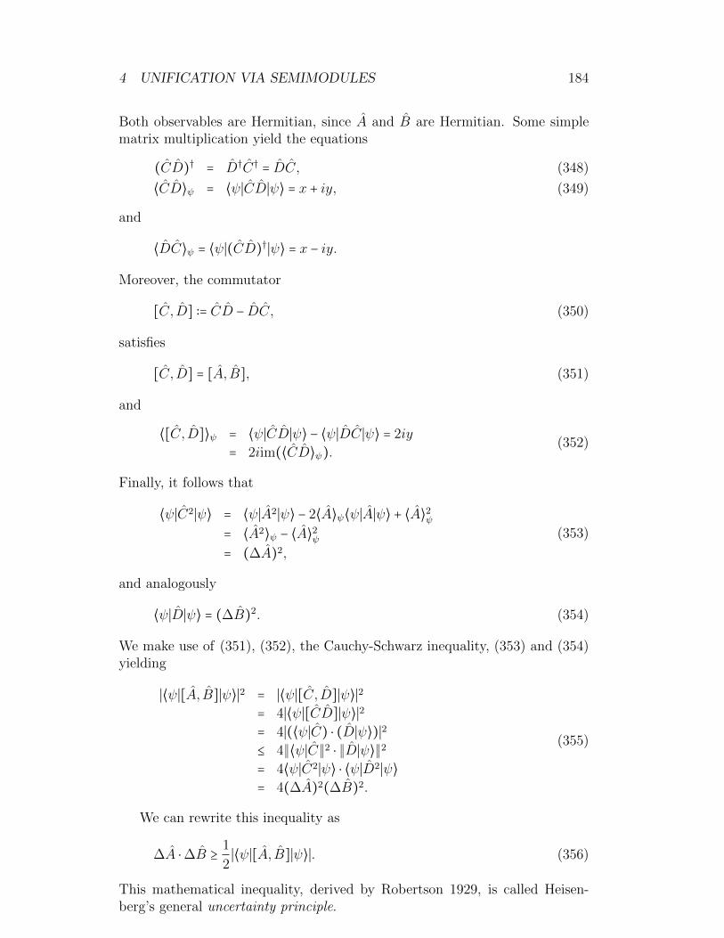
4 UNIFICATION VIA SEMIMODULES 184

Both observables are Hermitian, since A and B are Hermitian. Some simplematrix multiplication yield the equations

(CD)† = D†C† = DC, (348)

⟨CD⟩ψ = ⟨ψ∣CD∣ψ⟩ = x + iy, (349)

and

⟨DC⟩ψ = ⟨ψ∣(CD)†∣ψ⟩ = x − iy.

Moreover, the commutator

[C, D] ∶= CD − DC, (350)

satisfies

[C, D] = [A, B], (351)

and

⟨[C, D]⟩ψ = ⟨ψ∣CD∣ψ⟩ − ⟨ψ∣DC ∣ψ⟩ = 2iy

= 2iim(⟨CD⟩ψ).(352)

Finally, it follows that

⟨ψ∣C2∣ψ⟩ = ⟨ψ∣A2∣ψ⟩ − 2⟨A⟩ψ⟨ψ∣A∣ψ⟩ + ⟨A⟩2ψ

= ⟨A2⟩ψ − ⟨A⟩2ψ

= (∆A)2,

(353)

and analogously

⟨ψ∣D∣ψ⟩ = (∆B)2. (354)

We make use of (351), (352), the Cauchy-Schwarz inequality, (353) and (354)yielding

∣⟨ψ∣[A, B]∣ψ⟩∣2 = ∣⟨ψ∣[C, D]∣ψ⟩∣2= 4∣⟨ψ∣[CD]∣ψ⟩∣2= 4∣(⟨ψ∣C) ⋅ (D∣ψ⟩)∣2≤ 4∥⟨ψ∣C∥2 ⋅ ∥D∣ψ⟩∥2

= 4⟨ψ∣C2∣ψ⟩ ⋅ ⟨ψ∣D2∣ψ⟩= 4(∆A)2(∆B)2.

(355)

We can rewrite this inequality as

∆A ⋅∆B ≥ 1

2∣⟨ψ∣[A, B]∣ψ⟩∣. (356)

This mathematical inequality, derived by Robertson 1929, is called Heisen-berg’s general uncertainty principle.

4 UNIFICATION VIA SEMIMODULES 185

Since variances are always nonnegative, this inequality is meaningless andhas no content if the commutator [A, B] = 0. A well-known mathematical the-orem says that this commutator vanishes if and only if the sets of eigenvectorsof A and B are equal.

If on the other hand both observables do not commute, that is, their com-mutator [A, B] does not vanish, one cannot know the value of both observablesat once exactly. Or expressed in another way: knowing the value of one ob-servable precisely, makes the other observable completely vague. This can onlyhappen in quantum theory, where various orthonormal bases are allowed.

Now we apply this uncertainty principle to the Pauli matrices. Rememberthat we have derived these matrices by considering a macroscopic problem,namely to position a soccer ball on a spherical surface. It is a straightfor-ward matrix-matrix multiplication to compute the commutator for the Paulimatrices (282), (283) and (284):

σx, σy = [σxσy] − σyσx = 2iσz, [σy, σz] = 2iσx, [σz, σx] = 2iσy. (357)

Let

∣ψ⟩ = ψ0∣0z⟩ + ψ1∣1z⟩, ψ0, ψ1 ∈ C, ∣ψ0∣2 + ∣ψ1∣2 = 1 (358)

be a general state of the two-state system. Then

⟨ψ∣[σz, σx]∣ψ⟩ = ⟨ψ∣2iσy ∣ψ⟩= 2i {(ψ∗0)2⟨0z∣σy ∣0z⟩ + ψ∗0ψ1⟨0z∣σy ∣1z⟩

+ψ∗1ψ0⟨1z∣σy ∣0z⟩ + (ψ∗1)2⟨1z∣σy ∣1z⟩} .(359)

Since

σy ∣0z⟩ = (0 −ii 0

)(10) = (0

i) , (360)

and

σy ∣1z⟩ = (0 −ii 0

)(01) = (−i

0) , (361)

it follows

⟨ψ∣[σz, σx]∣ψ⟩ = 2i{(ψ∗0)2 ⋅ 0 + ψ∗0ψ1(−i) + ψ0ψ∗1 i + (ψ∗1)20}= 4 im(ψ∗0ψ1)

(362)

From (355) we obtain the uncertainty principle

∆σz ⋅∆σx ≥ im(ψ∗0ψ1). (363)

When ψ0 or ψ1 vanishes, the right hand side is zero, and this inequality isirrelevant. But otherwise we obtain a lower limit for the product of the uncer-tainties of σz and σx. In the case ψ0 = 1/

√2 and ψ1 = i/

√2 we get

∆σz ⋅∆σx ≥1

2. (364)

4 UNIFICATION VIA SEMIMODULES 186

Let us investigate the meaning of Heisenberg’s uncertainty principle forour macroscopic problem. From equation (280) it follows that ∣ψ⟩ = ∣0y⟩. Thisdenotes one half that results from bisecting the sphere with the xz-plane whichis perpendicular to the y-axis. We remember that the observables σz and σxlabel the two halves that result from bisecting the sphere with the xy-planeand the yz-plane, respectively. The area of the halve ∣0y⟩ contains parts of allareas ∣0z⟩, ∣1z⟩, ∣0x⟩, and ∣1x⟩. Hence, the knowledge that a ball is positionedon the surface of ∣0y⟩ does not determine whether the ball is above or belowthe xy-plane or above or below the yz-plane. In other words, if in a futureaction we would position a ball in the half ∣0y⟩, then it is uncertain if the ballwould be above or below the xy-plane or above or below the yz-plane. This isthe content of the uncertainty principle in this case. It is simple, not weird orparadox, clear from the geometry, supports our view that quantum mechanicsis the theory of the future, and applies also to macroscopic problems.

4 UNIFICATION VIA SEMIMODULES 187

4.18 Position-Momentum Commutation Relation

For understanding the position-momentum commutation relation it is perhapsthe best to go back to an idea of the electrical engineer Heaviside (1850-1925).He observed that differential operators often can be processed as numbers.This fact can be used to solve certain types of differential equations via simplealgebraic equations.

If we want to solve the differential equation

2y(x) + d

dxy(x) = h(x), (365)

we can treat the differential operator ddx as an ordinary number and write the

equation in the form

(1 + 1

2

d

dx) y(x) = 1

2h(x). (366)

Formally, we can divide through (1 + 12ddx) and apply the geometric series

corresponding to the term 12ddx . Then we get

y(x) = 1

2(1 − 1

2

d

dx+ 1

4

d2

dx2− 1

8

d3

dx3+ . . .)h(x). (367)

If we set for example h(x) = 2x3, then we find the solution

y(x) = x3 − 3

2x2 + 3

2x − 3

4. (368)

This formal procedure can be used in various applications. In particular, itcan be viewed as a key procedure in quantum mechanics.

Heaviside was confronted with declination and opposition. Of course, whentreating operators as numbers one must be very careful, because numberscommute, but in general operators don’t commute. If we think of x and d

dx

as operators, namely multiplication and differentiation operators that act onfunctions ψ(x), then

( ddxx − x d

dx)ψ(x) = d

dx(xψ(x)) − x d

dxψ(x) = ψ(x). (369)

Hence, both operators don’t commute and satisfy the commutation relation

d

dxx − x d

dx= 1, (370)

where 1 denotes the identity operator. In first order for small d

ψ(x + d) = ψ(x) + d ddxψ(x). (371)

Thus the differential operator ddx generates an infinitesimal translation x →

x+d. If ψ describes the state function of any object, then there are two cases toconsider. Either the object is transported through a distance d, then we speak

4 UNIFICATION VIA SEMIMODULES 188

of an active transformation, or the object is at rest and the origin of coordinatex is displaced by −d. The latter case is called a passive transformation.

Infinitesimal translations of a system in an n-dimensional configurationspace are closely related to what we mean by momentum, and thus not sur-prisingly in quantum mechanics the differential operators in generalized coor-dinates

Pj = −ih∂

∂qj(372)

describe the linear momentum. The operator Pj is called the momentum op-erator and acts on state functions that are elements in an appropriate Hilbertspace. The momentum operator coincides with the same interpretation as inclassical mechanics, where momentum can be viewed as the generator of trans-lations. Planck’s constant h has the dimension of the product of position andmomentum. Since we differentiate with respect to ∂

∂qj, thus dividing by posi-

tion, we should multiply with a product of position and momentum in orderto obtain the dimensions of momentum. This is the reason for multiplyingthe differentiation operator with Planck’s constant. The complex factor i isintroduced to ensure that the momentum operator is Hermitian, thus implyingreal measurable values.

If we are interested in the position of a particle or a system, then in quantummechanics position states ∣qk⟩ are introduced that describe the kth positioncoordinate as a Dirac delta function, that is,

∣qk⟩ = δ(q′k − qk). (373)

The position operator Qk is defined as the Hermitian operator69 which has theposition eigenvalues qk, that is,

Qk∣qk⟩ = qk∣qk⟩, (374)

where the position coordinate qk runs continuously from −∞ to ∞.Exactly as deriving (370), we find immediately the commutation relations

for the momentum operators Pj and the position operators Qk, that multipliesa function ψ with the position qk:

[Pj, Pk] = [Qj, Qk] = 0, [Pj, Qk] = −ihδjk1. (375)

The commutation relation is one of the most fundamental equations in physics.For example, the typical values of an electron in a hydrogen atom are 5×10−11

m for the position coordinate describing the radius, and 2×10−24 kg × m/s forthe momentum. Planck’s constant has the value

h = 1.054 × 10−34kg m2/s, (376)

that is close to the product of the radius and the momentum. These are verysmall quantities, and the commutation relation [Pj, Qj] = −ih1 shows that

69For a derivation and more details about position and momentum operators see Susskind[2014, Chapter 8], Penrose [2005, Chapter 21], or Schiff [1968, page 175].

4 UNIFICATION VIA SEMIMODULES 189

there is a small difference between PjQj and QjPj. However, what is small?Smallness has not an absolute meaning, but makes sense only when comparingobjects. Our units kg, m, and s are natural to us, because in daily life we aresurrounded by big objects consisting of more than 1026 atoms. But why arewe so big? Well, to obtain living and functioning objects, such as planets oranimals, requires a lot of atoms, moving slowly. But when looking at smallobjects like atoms, Planck’s constant becomes really large.

Now we can apply the uncertainty principle (356) using the commutationrelation (375). Then we obtain

∆Qj∆Pj ≥1

2h (377)

In particular, we see that for the position-momentum pair the uncertaintyprinciple turns out to be state independent. The interpretation is similar asabove. If we would know in the future the exact position of a particle, thenits momentum would be completely undetermined. The same holds true tothe momentum. Formulated in terms of machines: if the momentum is knownexactly, then all positions of the position machines are possibilities.

Finally, it should be mentioned that there is a very interesting, beautifulwritten, and extensive physic book by Schiller 70 where he investigated inpart IV “The Quantum of Change”. This book is highly recommendable forstudents in engineering. His starting thesis is:

• the action values S(t) and S(t + ∆t) between two successive events ofa quantum system, a time ∆t apart, cannot vanish. Roughly spoken,action is energy E times time t. More precisely, they satisfy the inequality

∣S(t +∆t) − S(t)∣ ≥ h2. (378)

This minimum action principle is in complete contrast to classical physics andhas never failed a single test, as pointed out in his book. He writes that itwould perhaps be better named the quantum of change.

He derives from this action principle in a modest manner several spectacularstatements using only simple mathematics. Formula (378) takes the form

∣(E ±∆E)(t +∆t) −Et∣ = ∣E∆t ±∆Et ±∆E∆t∣ ≥ h2. (379)

If we choose a suitable coordinate system, we can set E and t equals to zero,yielding

∆E∆t ≥ h2, (380)

when ∆E is the change of the energy of the system, and ∆t is the time betweentwo successive events. This inequality is called the time-energy uncertaintyprinciple, which is derived from the minimum action principle (378).

70Schiller [2016]

4 UNIFICATION VIA SEMIMODULES 190

For a free system with momentum p and mass 1, we can choose a coordinatesystem such that E = 0 but ∆E = ∆p2. Since for Cartesian coordinates x = qit is ∆x = ∆p∆t, the inequality (380) yield

∆p∆x ≥ h2, (381)

which is the position-momentum uncertainty principle. This is really a verysimple derivation of the uncertainty principle.

Based on the quantum of change, Schiller deduced several consequencesthat cannot be found in (all?) other textbooks:

• In nature there is no rest.

• In nature there is no perfectly straight or perfectly uniform motion.

• Perfect clocks do not exist.

• Motion backwards in time is possible over microscopic times and dis-tances.

• The vacuum is not empty.

• Photons have no position and cannot be localized.

• Microscopic systems behave randomly.

• Light can move faster than the speed of light c.

So what is the truth in physics?

5 QUANTIZATION AND FIELDS 191

5 Quantization and Fields

A field is a physical quantity that has a value for each point in space and time.This value may be a number, a vector, or an operator. Quantum Field The-ory (QFT) is a mathematical framework describing the extension of quantummechanics, dealing with a finite number of particles, to fields. Teller writes inthe preface of his well-known book 71:

QUANTUM FIELD THEORY is a notoriously hard theory tolearn. The best physics students do well with it, but many ablestudents flounder, eventually resigning themselves to going throughthe motions with their problem sets to make it through the course.Among philosophers of physics, I have heard many colleagues ex-press interest, only to learn a year or two later that they had some-how gotten involved in other things. I too have found the subjectextremely difficult, and after much effort, I have managed to un-derstand only some of the basics.

In fact, QFT is a really difficult subject. I hope that this section might helpstudents who have an interest in its conceptual structure and want to get aquick view of some basic ideas. An interesting survey can be found in the”Stanford Encyclopedia of Philosophy”.

The major goal of this section is to show that our imagination of machines,characterized by possibilities, and some results from the section about uni-fication via semimodules leads in a natural way to quantization and QFT.Moreover, we have to show that our physical model without an external timeparameter t is suitable for QFT.

QFT has grown successively in a very complex way, and its interpretationis sometimes notably weird. In contrast to many other physical theories QFTis not well-defined. Instead one can formulate several totally different modelsthat all have their merits but also limits. The most important applications arein particle physics. In particular, QFT describes scattering processes whereparticles are created while others are destroyed.

We start with the quantum harmonic oscillator. Its energy values are dis-crete in contrast to the classical harmonic oscillator possessing continuous en-ergy values. Moreover, the mathematical derivation of the quantum harmonicoscillator from the classical one is a perfect example of quantization. A har-monic oscillator can be viewed as a quantum field theory in one parametert, but without any space dimensions. We shall develop the quantization offields on the background of the simplest continuum theory, namely vibrationsof an atomic chain. This provides an entrance to quantum electrodynamicsand other quantum field theories.

71Teller [1997]

5 QUANTIZATION AND FIELDS 192

5.1 Quantization Rules

The word quantum comes from the Latin word quantus, which means ”howgreat”. In physics, this word is referred to the property that certain quantitiescan take on only discrete values. Quantization is known as the process ofconstraining continuous quantities, such as real or complex numbers, to adiscrete set, such as the integers. Hence, it is a little bit similar to discretizationas we shall see in Section 5.4.

Are there different processes of constraining quantities to discrete sets?What do these processes look like? Is there a common reason for quantization?

The first quantization rule is due to Planck 1900 who postulated the quanti-zation of energy E = nhω for his successful explanation of blackbody radiation.In order to understand certain properties of atoms Bohr 1913 postulated thatthe electron’s orbital angular momentum L = nh is quantized. Three yearslater Wilson and Sommerfeld offered a scheme that quantized the action of asystem. They derived Planck’s and Bohr’s postulates as special cases. Remem-ber, that we have mentioned this scheme and consequences already in Section4.18

Today, it is common to quantize a physical system by replacing the classicaldynamical variables by means of Hermitian operators. It is a recipe thattakes us from the Hamiltonian formalism of classical mechanics to quantumtheory. This scheme, called canonical quantization, comprises the previousquantization rules. At a first glance this recipe sounds really strange as Penrosewrites:

In fact, it seems to be mathematically completely crazy! ...What are we to do with this crazy-looking operator/momentum?The role of this ’quantum-mechanical momentum’, ih ∂

∂xa , is that itis to be slotted into the classical Hamiltonian function H(p1, ..., pN ;x1, ..., xN),just where the old classical momentum pa used to be. This is thekey to the procedure known as (canonical) quantization. Penrose2004, Chapter 21.2

From the point of view of Section 4, however, this replacement turns out tobe rather natural and not strange. There we started with the basic question

What are the base states of a physical model?

When answering this question, it was easy to define states and observables.Our initial situation are the classical dynamical variables: position q, mo-

mentum p, and functions F (p, q), like energy or angular momentum. Forexample, the one-dimensional harmonic oscillator has the energy functionH(p, q) = p2/2m +mω2q2/2. Position and momentum can be represented asregisters, that is, a sequence of binary questions. Each real value can beapproximated sufficiently accurate by a finite register. Both, position and mo-mentum, are observables that map the registers to values p and q, respectively.Now we go to the equivalent vector representation. Then the registers becomebase states ∣p⟩ and ∣q⟩, and the observables become diagonal matrices P and

5 QUANTIZATION AND FIELDS 193

Q with respect to their base states. The values q and p are the eigenvalues ofthese observables72.

In classical mechanics we have shown that there exists exactly one orthonor-mal basis. Hence, both observables P and Q are diagonal matrices with valuesp and q on the diagonal. They contain all information about position andmomentum. Diagonal matrices commute. The obvious way to get all valuesF (p, q) is to replace the values p and q by the diagonal matrices P and Q, suchthat we obtain the observable F = F (P , Q). This is the diagonal matrix withall classical values F (p, q) on the diagonal, thus containing all information.

In quantum mechanics the probabilistic theory of the future, the orthonor-mal basis of position vectors and the basis of momentum vectors are different,as we have seen. From (375) we obtain a non-zero commutator [P , Q] = ih.Hence, if we use the same idea and take the observable F = F (P , Q) we cannotexpect to obtain the eigenvalues F (p, q). We must carefully incorporate thecommutator. Then some simple manipulations give us the eigenvalues andeigenvectors of F . It turns out that the eigenvalues are quantized and do notcoincide with the classical values. Quantization is the result of some inevitablemathematical calculations using the commutation relations, but not of certainad hoc postulates.

However, due to the fact of non-commuting operators, the replacement ofdynamical variables by Hermitian operators is not obvious. Already the simpleclassical product term qp may be written as pq or 0.5(qp+pq). When replacingthese expressions by non-commuting operators they lead to different results.This problem is called the factor-ordering problem. One helpful way to find thecorrect operator expressions is to use Poisson brackets; the interested readeris referred to the rich literature.

Keep in mind: Quantization is the process of constraining con-tinuous quantities, such as real or complex numbers, to a discreteset. In canonical quantization the classical dynamical variablesposition and momentum in expressions are replaced by the Her-mitian position and momentum operators. Due to the fact thatoperators don’t commute, dynamical values are quantized. This re-placement must be done carefully, since the factor-ordering problememerges. Canonical quantization comprises the well-known quan-tization rules of Planck, Bohr, Sommerfeld, and Wilson. The un-derlying reason of quantization is the fact that quantum mechanicshas various orthonormal bases in contrast to classical mechanicsand classical probabilistic mechanics.

72If all possible values for q would be discrete, the eigenvalue problem can be written downin the usual form. But if q is a continuous real variable, then in order to be mathematicalrigorous, we require distribution theory. However, there is a way to avoid this theory. Therational numbers, dense in the set of real numbers, are countable, that is, there exists aninjective map from the set of rational numbers to the natural numbers. Hence, if we assumethat the position values q are rational, then we can replace q by an integer j(q), and canwrite the eigenvalue problem for Q in the form Q∣j(q)⟩ = q∣j(q)⟩. The same holds true forthe momentum. An advantage is that we can work with vectors indexed by natural numbersand can avoid integrals.

5 QUANTIZATION AND FIELDS 194

So far states, superpositions, and probabilities, thus many basic ingredientsof quantum mechanics, are not employed in the process of canonical quanti-zation. Quantization works in a rather general way. For example, it is well-known that the quantized classical equation of motion becomes the Heisenbergequation describing motion in quantum mechanics.

If we have a finite number of separate physical systems with position ob-servables Qj and momentum observables Pj for j = 1, ...,N , then we use thecommutation relations

[Pj, Ql] = ihδjl. (382)

for quantization.More general, we can replace the index j by rational or real index, say x

and t. Then we obtain the observables Q(x, t) and P (x, t). We use for fixed tthe commutation relations

[Q(x, t), P (y, t)] = ihδ(x − y) for all x, y. (383)

Now we have a rough impression of quantization. In the following wedescribe the details for several concrete systems.

5 QUANTIZATION AND FIELDS 195

5.2 Classical Harmonic Oscillator

A fundamental model in physics, perhaps the most important one, is the har-monic oscillator. This model is not a special physical pattern like that ofan electron or a fullerene molecule. Instead it is a mathematical model thatapplies to a large number of physical phenomena.

The harmonic oscillator describes particles moving under a restoring forcewhich pulls a particle back to the equilibrium position. Think of a spring, or aball moving inside a basin. Many physical systems can be described, at leastapproximately, by a quadratic energy function. When the system is disturbedout of the equilibrium it will oscillate. The atoms in crystals are an example ofoscillations. A wave is a disturbance or oscillation that travels through matteror space, and transfers energy and momentum. Mechanical waves propagate,due to a disturbance, through a medium by a deformation of the correspondingsubstance. The deformation leads to certain restoring forces. For instance,sound waves propagate via air molecules that collide with their neighbors andoscillate. However, electromagnetic waves, consisting of periodic oscillationsof electrical and magnetic fields generated by charged particles, are assumedto travel through a vacuum without any substance. Mathematically, it turnsout that the energy function of the electromagnetic field can be written as thesum of infinitely many harmonic oscillators. The quantization of a field canbe viewed as the quantization of its harmonic oscillators.

Let’s work through the harmonic oscillator. The total energy of a non-damped, simple harmonic oscillators is described by the Hamiltonian

H(p, q) = p2

2m+ 1

2κsq

2, (384)

that is, the total energy is the sum of kinetic and potential energy. The vari-ables q and p are the position and conjugate momenta coordinates, respectively,and κs denotes the spring constant.

The classical trajectory of motion in the phase space with coordinates(qk, pk) is described by two coupled differential equations of first order, calledthe Hamilton equations

pk = −∂H

∂qk, qk =

∂H

∂pk. (385)

Hence, given any Hamilton function and the values of the position and mo-menta coordinates at t, the equations (385) give the coordinates an infinites-imal time later. The complete trajectory in the phase space is obtained bysuccessively updating the coordinates. Remember that in our interpretationt is a geometrical parameter describing the oscillator’s trajectory in explicitform.

For the Hamiltonian (384) we obtain from (385) the equations

q = p

m, p = −κsq, (386)

yielding the equation

mq + κsq = 0. (387)

5 QUANTIZATION AND FIELDS 196

P

p2

p1Q0

Figure 77: The ellipse describes a certain orbit of a harmonic oscillator in atwo-dimensional phase space Q × P , consisting of the Cartesian product of aone-dimensional position space Q and a one-dimensional momentum space P .The grey area corresponds to the momentum interval p1 ≤ p ≤ p2 in the phasespace, and the pointed area is the position set q ≥ 0.

Frequently, the spring constant is written in the form

κs =mω2, (388)

and the Hamiltonian becomes

H(q, p) = p2

2m+ mω

2

2q2. (389)

Then the general solution is given by the functions

q = A cos(ωt − ϕ) and p =mq = −mAω sin(ωt − ϕ) (390)

with amplitude A, angular frequency ω, phase ϕ, and mass m. In Figure77 the motion of an harmonic oscillator is described in phase space. Thisgeometric form is similar to Kepler’s laws for planetary motion which are alsodescribed by functions, namely ellipses.

If we change the position variable q′ = (κsm)1/2q, then the Hamiltoniantakes the form

H = 1

2m(p2 + (q′)2). (391)

Hence, the Hamiltonian has a circle symmetry between the coordinates p andq. In the phase-space with q and p coordinates the harmonic oscillator circlesaround the origin. This can be described by the symmetric group of rota-tions. Notice the almost complete symmetry of Hamilton’s equations (385).

5 QUANTIZATION AND FIELDS 197

The minus sign in the second equation is the only asymmetry in Hamilton’sformulation.

For later purposes it is useful to write the Hamiltonian in product form.Let

α =√mω

2hq + i 1√

2hmωp, (392)

α† =√mω

2hq − i 1√

2hmωp, (393)

then we get the real quantity

α†α = mω2h

q2 + 1

2hmωp2 − i 1

2hqp + i 1

2hpq. (394)

Since the numbers qp commute, the Hamiltonian can be written as a productof complex coefficients:

H = hωα†α. (395)

It is useful to view the solutions (390) in the complex plane with realposition q-axis and imaginary momentum p-axis. From (390) and (393) itfollows that the complex amplitude evolves as

α†(t) =√mω

2hA cos(ωt−ϕ)−i 1√

2hmωmAω sin(ωt−ϕ) = (A

√mω

2heiϕ) e−iωt.

(396)

In this plane the solutions can be visualized as a clockhand rotating clockwisewith frequency ω.

5 QUANTIZATION AND FIELDS 198

5.3 Quantum Harmonic Oscillator

It is natural to view the oscillator as a machine described by its mutually ex-clusive alternatives, the base states, and corresponding numbers that describethe positions and momenta. This is the concept of an observable. Now, whatare the base states? We applycanonical quantization.

We insert the operators P and Q into the classical Hamiltonian (389) andlook what happens. For the harmonic oscillator we obtain the so-called Hamil-ton operator

H = 1

2mP 2 + 1

2mω2Q2. (397)

This operator is Hermitian. Because formula (397) contains the necessaryinformation about all positions and momenta, it should contain all energyeigenvalues and energy base states of the oscillator.

Quantization is a purely algebraic way solely based on the commutationrelation for the position and momentum operator discussed in Section 4.18:

[P , Q] = P Q − QP = −ih (398)

No further information is required to obtain all energy eigenvalues and eigen-states of the Hamilton operator.

We try to rewrite (397) as a product of two operators. Finding the eigenval-ues of a product of operators is much easier than of their sum. For numbers wehave factorized a sum in (394), (395) using complex numbers. But in contrastto complex numbers, operators don’t commute, and we have to take accountof the commutator (398). Using our rule of canonical quantization, accordingto (393) we define the two operators

A =√mω

2hQ + 1√

2hmωiP , (399)

A† =√mω

2hQ − 1√

2hmωiP . (400)

The operator A is called the annihilation operator, and A† is called the creationoperator. Their names will become clear below. Reversely, we obtain

Q =√

h

2mω(A† + A), P = i

√mhω

2(A† − A), (401)

Some simple calculations using the commutation relations (398) yield

[A, A†] = 1, [A, A] = 0, [A†, A†] = 0. (402)

Multiplying out we get

H = 1

2hω(AA† + A†A) = hωN + 1

2hω1, (403)

5 QUANTIZATION AND FIELDS 199

where the operator N = A†A is called number operator. This factorization isonly possible when using complex numbers. Real numbers are not sufficient.This is a further argument for the need of complex numbers.

Obviously, the number operator satisfies the commutation relations

[N , A†] = A†, [N , A] = −A. (404)

Moreover, the commutation relations

[H, A†] = hωA†, [H, A] = −hωA, [H, N] = 0. (405)

follow immediately. The equations (402) and (405) show that the set of op-erators 1, A, A† and H is closed under the commutation operation, and suchsets are called commutator algebras. Now we show the power of the commuta-tor algebra: it solves the eigenvalue problem of the Hamilton operator (397).This operator is Hermitian, and thus has an orthonormal basis of eigenvectors∣n⟩ with observable energy eigenvalues En. Since the Hamiltonian H and thenumber operator N commute, they have the joint set of eigenvectors {∣n⟩}.

Firstly, let En, ∣n⟩ be an arbitrary eigenpair, that is,

H ∣n⟩ = En∣n⟩. (406)

Then using the previous commutation relations, we obtain

HA†∣n⟩ = (A†H + hωA†)∣n⟩ = (En + hω)A†∣n⟩, (407)

HA∣n⟩ = (AH − hωA)∣n⟩ = (En − hω)A∣n⟩. (408)

Therefore, we see that for each eigenvector ∣n⟩ the vectors A†∣n⟩ and A∣n⟩ are(unnormalized) eigenvectors of H and N with energy eigenvalues En + hω andEn − hω, respectively.

Secondly, if we repeat this process, we obtain a sequence of eigenpairs witheigenvalues

. . . ,En − 3hω,En − 2hω,En − hω,En,En + hω,En + 2hω,En + 3hω, . . . (409)

and unnormalized eigenvectors. Since the Hamiltonian is the sum of twosquared Hermitian operators, all eigenvalues En are nonnegative. Becauseof (403), the previous process stops, if the energy value E0 = hω/2 occurs.Therefore, in contrast to the classical harmonic oscillator, we obtain a lowestpositive energy.

Thirdly, since the lowest energy value satisfies E0 = hω/2, the expression in(409) vanishes if and only if En = E0. The value E0 is the ground state energycorresponding to the ground state ∣0⟩. For the ground state the equation

A∣0⟩ = 0. (410)

must be satisfied, since otherwise (408) would imply negative eigenvalues ofthe Hamiltonian. All eigenvalues of the Hamiltonian operator are

En = hω(n +1

2), n = 0,1,2, . . . (411)

5 QUANTIZATION AND FIELDS 200

If there would be another eigenvalue, we apply the previous steps of creationand annihilation to this eigenpair, yielding an eigenvector with eigenvaluesmaller than E0, what is impossible. Summarizing, we have obtained withthe commutation relations the complete energy spectrum of the harmonic os-cillator, which is discrete with a positive lowest energy. This seems to be aweird property from the point of view of classical mechanics, where the energyspectrum is continuous with lowest value zero.

Finally, using (403) and (411), it follows that

N ∣n⟩ = A†A∣n⟩ = ( 1

hωH − 1

2) ∣n⟩ = ( 1

hωEn −

1

2) ∣n⟩, (412)

and hence

N ∣n⟩ = n∣n⟩. (413)

This is the reason why the operator N is called number operator, see Figure78.

n = 6n = 5n = 4n = 3n = 2n = 1n = 0

AA

Figure 78: The energy levels of the harmonic oscillator are discrete and canbe visualized as a ladder. The operators A† and A raise and lower the energylevel, respectively, and thus explains their names. The number operator N hasthe lower bound zero corresponding to the ground state, but no upper bound.

Since A∣n⟩ is an eigenvector of the number operator and

NA∣n⟩ = AN ∣n⟩ + [N , A]∣n⟩ = An∣n⟩ − A∣n⟩ = (n − 1)A∣n⟩, (414)

it follows that A∣n⟩ is an eigenvector of N corresponding to the eigenvaluen−1. Thus it must be (up to a normalization constant) the eigenvector ∣n−1⟩.We set

A∣n⟩ =√n∣n − 1⟩. (415)

Analogously, we obtain

A†∣n⟩ =√n + 1∣n + 1⟩. (416)

5 QUANTIZATION AND FIELDS 201

With the square root factors the equation (413) is fulfilled In particular, wecan express all base states by acting repeatedly on the ground state ∣0⟩ withthe creation operator:

∣1⟩ = A†∣0⟩, ∣2⟩ = 1√2A†∣1⟩ = 1√

2(A†)2∣0⟩, ... (417)

and more general

∣n⟩ = 1√n!

(A†)n∣0⟩. (418)

We have found all eigenvalues and all orthonormal eigenvectors of theHamilton operator. The eigenvectors (418) form a set of distinguishable basestates. The approach to work with non-commutative operators in-stead of commutative numbers has lead us to quantization: the spec-trum of the Hamiltonian is infinite, but discrete. To obtain thisresult we have used the operators H, N , A, A† that act on base statestogether with their commutation relations. Unitary transformationsacting on superposed states are not involved.

We can represent these operators as matrices related to the basis of or-thonormal energy eigenvectors {∣n⟩}. Since an operator M can be describedby a matrix with coefficients

Mn′n = ⟨n′∣M ∣n⟩, (419)

it follows that the Hamilton operator is represented by an infinite diagonalmatrix with the energy eigenvalues (411) on the diagonal.

Formula (416) implies immediately that the creation and annihilation op-erators have the non-Hermitian matrix representations

A†n′n =

⎛⎜⎜⎜⎜⎜⎜⎝

0 0 0 0 . . .√1 0 0 0 . . .

0√

2 0 0 . . .

0 0√

3 0 . . .⋮ ⋮ ⋮ ⋮ ⋯

⎞⎟⎟⎟⎟⎟⎟⎠

, An′n =

⎛⎜⎜⎜⎜⎜⎜⎝

0√

1 0 0 . . .

0 0√

2 0 . . .

0 0 0√

3 . . .0 0 0 0 . . .⋮ ⋮ ⋮ ⋮ ⋯

⎞⎟⎟⎟⎟⎟⎟⎠

(420)

All these matrices are infinite dimensional. However, since energy is neverinfinite, we can view these as large finite-dimensional matrices.

Since the harmonic oscillator is perhaps the most fundamental physicalmodel, it is interesting for understanding quantum mechanics to investigatethe Hermitian matrix representations of the most important observables. Thenumber operator (413) has the representation

N =

⎛⎜⎜⎜⎜⎜⎜⎝

0 0 0 0 . . .0 1 0 0 . . .0 0 2 0 . . .0 0 0 3 . . .⋮ ⋮ ⋮ ⋮ ⋯

⎞⎟⎟⎟⎟⎟⎟⎠

(421)

5 QUANTIZATION AND FIELDS 202

From (401) we obtain the matrix representations of the position and momen-tum operator

Q =√

h

2mω

⎛⎜⎜⎜⎜⎜⎜⎝

0√

1 0 0 . . .√1 0

√2 0 . . .

0√

2 0√

3 . . .

0 0√

3 0 . . .⋮ ⋮ ⋮ ⋮ ⋯

⎞⎟⎟⎟⎟⎟⎟⎠

, P = i√

mhω

2

⎛⎜⎜⎜⎜⎜⎜⎝

0 −√

1 0 0 . . .√1 0 −

√2 0 . . .

0√

2 0 −√

3 . . .

0 0√

3 0 . . .⋮ ⋮ ⋮ ⋮ ⋯

⎞⎟⎟⎟⎟⎟⎟⎠

.

(422)

These matrices should satisfy the commutation relations (398), and thus theposition-momentum uncertainty principle. In fact, some simple computationsshow

QP = i h2

⎛⎜⎜⎜⎜⎝

1 0 −√

2 . . .0 1 0 . . .√2 0 1 . . .⋮ ⋮ ⋮ ⋯

⎞⎟⎟⎟⎟⎠

, P Q = i h2

⎛⎜⎜⎜⎜⎝

−1 0 −√

2 . . .0 −1 0 . . .√2 0 −1 . . .⋮ ⋮ ⋮ ⋯

⎞⎟⎟⎟⎟⎠

, (423)

implying the desired result P Q − QP = −ih.

ψ3

ψ2

ψ1

ψ0

|ψ3|2

|ψ2|2

|ψ1|2

|ψ0|2

Figure 79: The first four wave functions ψi with corresponding probabilitydensities ∣ψ2

i ∣.

So far we have described algebraic consequences of the commutation re-lations and the quadratic form of the Hamilton operator. In particular, we

5 QUANTIZATION AND FIELDS 203

have found all important algebraic facts about this operator. It’s eigenvaluesare quantized. What has all this to do with quantum mechanics, known asa stochastic process? Nothing. Until now this theory is deterministic sinceonly distinguishable base states are used. Hence, it belongs more to classicaldeterministic mechanics, not to the stochastic part of quantum theory. Quan-tization is the process of finding base states, the fundamental building blocksof the future, present, and past.

The Hamilton operator is defined via the position and momentum operator.Hence, when inserting both operators in their position representation, it shouldbe possible to obtain the eigenfunctions ∣ψn(x)⟩ = ∣n⟩ corresponding to theenergy eigenvalues. Here, we use Cartesian coordinates x as usual. Then forthe lowest energy level the equation (410) in position representation has theform

⎛⎝

√mω

2hx + i

√1

2mhω

h

i

∂

∂x

⎞⎠ψ0(x) = 0. (424)

It is easy to see that

ψ0(x) = 4

√mω

πhe−

mω2hx2 (425)

is a solution. Moreover it is a normalized solution, because the integral overspace ∫

∞

−∞ψ∗0(x)ψ0(x)dx = 1. With (418) all other eigenfunctions can be ob-

tained:

ψn(x) =1√n!

⎛⎝

√mω

2h+ i

√1

2mhω

h

i

∂

∂x

⎞⎠

n

ψ0(x). (426)

Some computations that can be found in most textbooks about quantum me-chanics yield the normalized wave functions

ψn(x) = 4

√mω

hπ

1√2nn!

e−mωh

x2

2 Hn (√mω

hx) (427)

where Hn are the Hermitian polynomials, see Figure 79 for the first four wavefunctions. The corresponding formulas are:

ψ0 = (aπ)

14

e−y2/2,

ψ1 = (aπ)

14 √

2ye−y2/2,

ψ2 = (aπ)

14 1√

2(2y2 − 1)e−y2/2,

ψ3 = (aπ)

14 1√

3(2y3 − 3y)e−y2/2,

(428)

where a = mωh

and y =√ax.

5 QUANTIZATION AND FIELDS 204

One can prove that these normalized functions are orthogonal, that is,

∫∞

−∞

ψ∗n(x)ψm(x)dx = 0 for n ≠m. (429)

Thus they form a set of distinguishable base states.In summary, we have shown that a purely algebraic method, solely based

on base states together with observables acting on base states, lead to thequantization of the energy values. Moreover, for the position representationwe have obtained the corresponding orthogonal eigenfunctions ψn(x). Theseare purely geometric objects and represent mutually exclusive alternatives. Itis most helpful to keep in mind that these function do not depend on time,thus they don’t require the (3+1)-spacetime.

But what can be the meaning of these timeless functions? What have thesefunctions to do with an oscillating object? Where does quantum probabilitycome into play? These functions are related to the position x of the oscil-lator. It is a good choice to interpret these functions probabilistic in termsof probability amplitudes defined on the position base states. The latter arethe mutually exclusive alternatives where the oscillator might be. As usualwe apply Born’s rule for obtaining the probabilities. This rule says that theprobability of finding the oscillator at any given position x is the square ofthe magnitude of the function ∣ψn(x)∣2. From formula (427) it follows thateach eigenfunction is an exponential function in x multiplied by a polynomial.Hence, as x→ ±∞ all eigenfunctions go to zero, and thus the probability thatthe mass moves far away from the equilibrium point goes to zero for each en-ergy value. It can be shown that each eigenfunction has one more real zero,if the energy is increased by one unit hω. Thus for increasing energies theeigenfunctions oscillate more rapidly. Moreover, the eigenfunctions spread outfor increasing energies.

If we think in terms of an oscillating ball, we can conclude that the zeros ofthe eigenfunctions are points where the oscillating ball will never be found. Forthe lower energy states the most probable values of position are different fromthe classical harmonic oscillator. Classically, the oscillator spends more timeclose at the turning points of its motion, since there its velocity is almost zero.This looks rather strange. But for increasing energies, the chance of beingfar away from the equilibrium point increases. Then the probability densitybecomes concentrated at the turning points of the classical oscillator, where theparticle spends most of its time, see Figure 79. In this context time means:when performing many experiments in most cases the oscillating particle isfound close to the turning points. In contrast to classical mechanics, it followsthat there is a small positive probability to find the ball outside the basin. Thiseffect is called quantum tunneling, an important physical phenomenon withmany applications, such as the tunnel diodes, scanning tunneling microscopeor quantum computing.

Thus, we have obtained a completely different picture of the quantum har-monic oscillator compared with the classical case. What is the reason for that?If the position and the momentum operator would be diagonal matrices, theircommutator would be zero, and nothing interesting would happen. Hence, the

5 QUANTIZATION AND FIELDS 205

commutation relations are the key to quantization. But what is the mathe-matical reason for the commutation relations? Obviously, this is caused by thefact that the underlying complex linear space allows different bases such thatthe operators cannot be simultaneously diagonalized.

Keep in mind: Replacing in the classical Hamiltonian the classi-cal variables position and momentum by their corresponding Her-mitian observables leads to the energy Hamilton operator. A purelyalgebraic method, based only on the commutation relations, showsthat the energy values are discrete, and thus justifies the namequantization. Hence, whenever you see operators, figure out theircommutators. The related base state functions do not depend on anexternal time parameter t, but have a probabilistic interpretation.

5 QUANTIZATION AND FIELDS 206

5.4 Matrix Mechanics in Position Representation

In Section 5.3 we have considered the matrix theory of the harmonic oscillatorin the energy representation. Moreover, we have presented position, momen-tum, energy, annihilation, and creation operators as matrices with respect tothe orthonormal energy eigenstates. It is a good exercise to investigate theseoperators with respect to other basis representations. In this section we con-sider the position representation. This provides a deeper understanding ofmatrix mechanics.

The classical dynamical variable position is the most natural quantity inphysics. Although this variable is continuous in classical mechanics, we con-sider a discrete one-dimensional position space, which may be defined via adiscrete coarse graining such that

q = n ⋅ ε, −N ≤ n ≤ N, (430)

with grid spacing ε > 0, and integer N which may also be infinite. The gen-eralization of the following investigation to higher dimensional infinite or con-tinuous position spaces is straightforward. Let the set of vectors

∣ψ⟩ ∶=N

∑n=−N

ψn∣n⟩, ψn ∈ C (431)

denote the position state space, where ∣n⟩ is the normalized basis vector cor-responding to the position q = nε. Then the coefficients ψ(n) = ψn are theamplitudes generating the corresponding wave function ∣ψ⟩. The squared mag-nitude of the amplitude is the probability of finding the particle in state ∣n⟩.The basis states ∣n⟩ are the orthonormal eigenvectors of the position operatorQ, that is

Q∣n⟩ = nε∣n⟩, ⟨n∣n′⟩ = δnn′ , (432)

and −N ≤ n,n′ ≤ N . Therefore, the matrix position representation of Q takesthe form

Qn′n = ⟨n′∣Q∣n⟩ = nεδn′n, (433)

and thus yields the diagonal matrix

Q = ε

⎛⎜⎜⎜⎜⎜⎜⎜⎜⎜⎜⎜⎜⎜⎜⎜⎝

−N⋱

−2 0−1

01

0 2⋱

N

⎞⎟⎟⎟⎟⎟⎟⎟⎟⎟⎟⎟⎟⎟⎟⎟⎠

. (434)

Its expectation value is

⟨Q⟩ψ = ⟨ψ∣Q∣ψ⟩ =N

∑n=−N

nε∣ψn∣2. (435)

5 QUANTIZATION AND FIELDS 207

The momentum operator P = −ih ∂∂q in position presentation can be obtained

via discretization by using centered differences, that is, we replace the differ-ential operator ∂

∂q by the difference operator ∆ε such that

∆

εψ(n) ∶= 1

2(ψ(n + 1) − ψ(n − 1)). (436)

Then

Pψ(n) = −ih∆

εψ(n) (437)

is an approximation of Pψ(q) = −ih∂ψ(q)∂q , where q = nε. Assuming periodic

boundary conditions ψ(−N) = ψ(N) such that the states ∣n⟩ may be viewedas discrete points on a circle, we obtain the momentum matrix

P = − ih2ε

⎛⎜⎜⎜⎜⎜⎜⎜⎜⎝

0 1 0 0 . . . −1−1 0 1 0 . . . 0

0 −1 0 1 . . . 00 0 −1 0 . . . 0⋮

1 0 0 0 . . . 0

⎞⎟⎟⎟⎟⎟⎟⎟⎟⎠

. (438)

As expected, the discretization yields a matrix with 1’s above and -1’s belowthe diagonal. Observe that both matrices Q and P are Hermitian matrices inthe energy representation (422) as well as in the position representation (434)and (438).

A simple computation yields the commutator

[Q, P ] = ih2

⎛⎜⎜⎜⎜⎜⎜⎜⎜⎝

0 1 0 0 . . . 01 0 1 0 . . . 00 1 0 1 . . . 00 0 1 0 . . . 0⋮0 0 0 0 . . . 0

⎞⎟⎟⎟⎟⎟⎟⎟⎟⎠

. (439)

Thus the matrix has 1’s above and below the diagonal. As the discretizationbecomes finer, the nonzero entries seem to be more and more concentrated atthe diagonal. But it is not an identity matrix as we expect from the commu-tation relation and (423). But the equation

[Q, P ]⎛⎜⎝

⋮ψ(n)⋮

⎞⎟⎠= ih

⎛⎜⎝

⋮12(ψ(n − 1) + ψ(n + 1))

⋮

⎞⎟⎠≈ ih

⎛⎜⎝

⋮ψ(n)⋮

⎞⎟⎠

(440)

shows that for a fine discretization this matrix behaves like an identity matrix,provided ψ is sufficiently smooth such that the arithmetic mean 1

2(ψ(n − 1) +ψ(n + 1)) is almost equal to ψ(n).

The eigenstates of the position operator in the position representation arethe positions q = nε of our coarse graining. What are the eigenstates ∣ψp⟩ of

5 QUANTIZATION AND FIELDS 208

the momentum operator in the position representation? Using the equation(438), the eigenvalue equation

P ∣ψp⟩ = p∣ψp⟩ (441)

can be written equivalently in the the componentwise form

− ih2ε

(ψp(n + 1) − ψp(n − 1)) = pψp(n). (442)

Dividing by ih yields the difference equation

ψp(n + 1) − ψp(n − 1)2ε

= i

hpψp(n), (443)

which is a discretization of the differential equation

∂ψp(q)∂q

= i

hpψp(q). (444)

The general solution of this equation is given by

ψp(q) = cppeipqh , (445)

where cp is constant.Summarizing, when taking the position representation, a discrete coarse

graining, and centered differences, the quantum observables are simple matri-ces and the differential equations are approximated by difference equation.

5 QUANTIZATION AND FIELDS 209

5.5 Several Harmonic Oscillators

In this section we consider the canonical quantization of N uncoupled harmonicoscillators as a preparation for more complicated problems. The oscillatorsmay be positioned at arbitrarily different places without any contact. Thus,their Hamiltonian takes the form

H =N

∑k=1

Hk, Hk =P 2k

2mk

+ 1

2mkω

2kQ

2k. (446)

From Section 5.3 it follows immediately that the kth oscillator can bedescribed by the creation operator A†

k and the annihilation operator Ak:

A†k∣n1, n2, . . . , nk, . . .⟩ =

√nk + 1 ∣n1, n2, . . . , nk + 1, . . .⟩,

Ak∣n1, n2, . . . , nk, . . .⟩ =√nk − 1 ∣n1, n2, . . . , nk − 1, . . .⟩.

(447)

Moreover, since the oscillators are separated, these operators satisfy the com-mutation relations

[Ak, Ak′] = 0, [A†k, A

†k′] = 0, [Ak, A†

k′] = δkk′ . (448)

Because of (446) and (403), the Hamiltonian in terms of these operators is

H =N

∑k=1

hωk (A†kAk +

1

2) . (449)

The vacuum state ∣0⟩ = ∣0,0,0, ...⟩ is the state where each oscillator is in itsground state such that

Ak∣0⟩ = 0 (450)

for all k. From formulas (418) and (447) we obtain the so-called occupationnumber representation of these oscillators

∣n1, n2, . . . , nN⟩ = 1√n1!n2!⋯nN !

(A†1)n1(A†

2)n2⋯(A†N)nN ∣0,0, . . . ,0⟩. (451)

The kth oscillator has nk quanta of energy.This simple generalization to several independent oscillators shall serve us

when considering more complicated problems. The results above can be imme-diately applied to a three-dimensional harmonic oscillator. It’s Hamiltonian isjust the sum of three one-dimensional Hamiltonians.

5 QUANTIZATION AND FIELDS 210

5.6 The Oscillator Chain

We consider a one-dimensional circular chain of radius R consisting of N atomswith identical masses m. The atoms are connected by springs with springconstant κs, as shown in Figure 80. For largeN the distance between two atomsin their equilibrium positions is a = 2πR/N , approximately. The displacementof the jth atom from the equilibrium position xj is denoted by qj.

The classical Hamiltonian of this chain is the sum of the kinetic and thepotential energy:

H(p, q) =N

∑j=1

[ 1

2mp2j +

κs2(qj+1 − qj)2] . (452)

The corresponding Hamilton equations are:

pj = −∂H∂qj

= κs(qj−1 − 2qj + qj+1),

qj = ∂H

∂pj=pjm.

(453)

Since pj =mqj we obtain for the jth atom the equation of motion:

mqj − κs(qj−1 − 2qj + qj+1) = 0, j = 1, . . . ,N. (454)

We consider a closed oscillator chain with periodic boundary conditions

qj+N(t) = qj(t), (455)

see Figure 80.In contrast to Section 5.5, we are now dealing with a problem where each

mass is strongly coupled to its neighbor by the springs. Thus, the atoms cannotbe considered independently. Surprisingly, it will turn out that the quantizedsystem behaves as a system of independent, uncoupled harmonic oscillators.

We solve equation (454) with the Ansatz

qj(t) = ei(jp−ωt), j = 1, . . . ,N. (456)

Substituted into the equations of motion, we obtain

[−mω2 − κs(e−ip − 2 + eip)] ei(jp−ωt) = 0. (457)

The boundary condition (455) requires for j = 0

ei(Np−ωt) = e−iωt. (458)

This can be satisfied if and only if p takes the discrete values

pk =2πk

N, k = 0,±1, . . . ,±N

2, (459)

where we have assumed that N is even. Since

e−ip − 2 + eip = −4 sin2 p

2, (460)

5 QUANTIZATION AND FIELDS 211

'

&

$

%

s

aR

Figure 80: A closed oscillator chain in rest position with spring constant κsand total lenght L = 2πR = Na.

equation (457) implies

−mω2 + κs4 ⋅ sin2 p

2= 0. (461)

If we set κs =mω20/4, then with (459) we obtain the dispersion relation

ω2k = ω2

0 sin2 (πkN

) , k = ±1, . . . ,±N2. (462)

We have excluded k = 0 since this case corresponds to a trivial constant dis-placement. At small momenta pk, where k is small compared to N , the lineardispersion law

ωk = 2

√κsm

∣k∣ (463)

is fulfilled.In summary, we have obtained for the jth atom the solution

qj(t) = ei(2πkjN

−ωkt), j = 1, . . . ,N, (464)

where the frequency ωk satisfies the dispersion relation (462). The solutionsqj describe an elementary vibrational motion in which a chain of N atomsuniformly oscillates at a fixed common frequency ωk, see Figure 81. There are

5 QUANTIZATION AND FIELDS 212

'

&

$

%Figure 81: A phonon.

N vibrational motions corresponding to the frequencies ωk. Each such motionis called a normal mode. The modes can be viewed as waves or excitationsrunning along the chain. A phonon is its quantum mechanical description, seethe next section. Phonons play a major role, for instance in condensed matterphysics. They are collective excitations in elastic arrangements of particles.

The general real solution for the jth atom, satisfying the equation of motion(454), can be written as the superposition of normal modes

qj(t) =1√N

N2

∑k=−N

2

ckei( 2πkj

N−ωkt) + c∗ke

−i( 2πkjN

−ωkt), j = 1, . . . ,N. (465)

This is a Fourier expansion. Combining modes in this way leads to travelingwaves, see Figure 82. In other words, motion can be analyzed by assumingthat it is the sum of different modes. A nice and very detailed description ofthis phenomenon is presented in the Feynman Lectures73.

73http://www.feynmanlectures.caltech.edu/I_49.html

5 QUANTIZATION AND FIELDS 213

'

&

$

%Figure 82: Motion as a superposition of normal modes.

5.7 Quantization of the Chain

We quantize the chain in the same manner as for the harmonic oscillator. Wereplace in (452) positions qj and momentum pj by the observables Qj and Pj,respectively. Obviously, these Hermitian operators satisfy the commutationrelations

[Pj, Ql] = ihδjl. (466)

Not surprisingly, several computations74 show that the Hamiltonian becomes

H =N2

∑k=−N

2

hωk (A†kAk +

1

2) (467)

where Ak and A†k are the creation and annihilation operators, respectively.

They satisfy the commutation relations

[Ak, Ak′] = [A†k, A

†k′] = 0, [Ak, A†

k′] = δkk′ . (468)

It follows that the closed harmonic chain is expressed as a sum of separatemodes k that behave like single harmonic oscillators.

The state ∣0⟩ = ∣0,0,0, ...⟩ denotes the ground state where

Ak∣0⟩ = 0 for all k = −N2, . . . ,+N

2. (469)

74For a proof see for example: Lancaster, Tom, and Stephen J. Blundell. Quantum fieldtheory for the gifted amateur. OUP Oxford, 2014. Chapter 2.4. We proof this later for themore difficult continuous oscillator chain.

5 QUANTIZATION AND FIELDS 214

A general base state

∣n1, n2, . . . , nN⟩ = 1√n1!n2!⋯nN !

(A†1)n1(A†

2)n2⋯(A†N)nN ∣0,0, . . . ,0⟩. (470)

contains nk elementary excitations of the normal mode k. These excitationsare obtained by applying nk times the creation operator A†

k to the groundstate. This formalism is called the occupation number representation withthe occupation numbers nk, namely the number of phonons that have thesame frequency ωk. As in the case of a single harmonic oscillator, the set ofbase states ∣n1, n2, . . . , nN⟩, that is the excitations, are the eigenstates of theHamilton operator. They are orthonormal vectors which span a Hilbert space,called Fock space. Because of (411), the chain’s total energy for the base state∣n1, n2, . . . , nN⟩ is

E =N2

∑k=−N

2

hωk (nk +1

2) . (471)

Using the commutation relations (468), it follows for N = 2 that

∣n1, n2⟩ =1√n1!n2!

(A†1)n1(A†

2)n2 ∣0,0⟩ = ∣n2, n1⟩. (472)

This means that the base states are symmetric under excitation exchange. Inparticle physics symmetric states are called bosons. It is easy to generalizethis symmetry to base states ∣n1, n2, . . . , nN⟩. The formalism, using creationand annihilation operators that act on the Fock space, provide a useful tool tostudy many-body systems.

Is there a difference between phonons, living as an excitation in a lattice likea solid state crystal, and photons, the excitations of the electromagnetic field?Not so much. The phonon can be viewed as a quantum of sound, for examplein a solid, whereas the photon is the quantum of electromagnetic radiation.Both are bosons. They are excitations described by waves. Moreover, bothhave an energy equal to their frequency times h. This is similar as in stringtheory, where particles are modes of strings.

5 QUANTIZATION AND FIELDS 215

5.8 The Field as a Continuous Limit

Until now we have considered only discrete systems. If the number of atomsgrows such that their spacing becomes very small, we obtain approximately acontinuous system, that is, a one-dimensional string of length

L = Na = 2πR. (473)

In the continuous limit we assume a finite mass density %

% =m/a, (474)

and a finite string tension

σ = κsa. (475)

Then

a,m→ 0, N, κs →∞, L, ρ, σ are constant, x = ja for j = 1, . . . ,N. (476)

Hence, the length L, the density ρ, and the tension σ are fixed. The dis-placements qj(t) transform into a continuous displacement field q(x, t). Thediscrete index is merely replaced by the continuous index x. Then differencesbecome derivatives, and sums are replaced by integrals:

qj(t) → q(x, t), (477)

(qj(t) − qj−1(t))2 → a2 (∂q(x, t)∂x

)2

, (478)

∑j

→ 1

a

L

∫0

dx, (479)

and therefore

N =N

∑j=1

1 = La= 1

a

L

∫0

1dx. (480)

From (452) it follows that the Hamiltonian, the sum of kinetic and potentialenergy, becomes

H(p, q) =L

∫0

dx [ 1

2%p2(x, t) + σ

2(∂q(x, t)

∂x)

2

] , (481)

where

p(x, t) = %∂q(x, t)∂t

(482)

is the canonical momentum. According to (454), the equation of motion is:

∂2q(x, t)∂t2

− c2∂2q(x, t)∂x2

= 0, c =√

σ

%= a

√κsm. (483)

This is a linear wave equation with propagation velocity c. The quantity c isa characteristic speed in a specific medium, thus not necessarily the speed oflight. The linearity implies that linear combinations of solutions are solutions.

5 QUANTIZATION AND FIELDS 216

5.9 Renormalization

Until now we have not quantized continuous systems, but it is obvious thatthere should be problems if the number of modes kn is infinite. In the contin-uum limit N →∞ the ground stage energy

E0 =N2

∑n=−N

2

1

2hωn =

h

2

∞

∑n=−∞

c

R∣n∣ (484)

is divergent.Such divergences occur often in QFT. Frequently, divergences appear when

going to the continuous limit and if interactions are occur. They require a phys-ical discussion, since calculations with infinities are not so funny, and continu-ous models are only physically relevant if such divergences are avoided. Thereare cut-off procedures, so-called renormalizations, that replace the infinitiesby finite values. For instance, such a cut off procedure may be motivated byassuming a physically relevant particle number.

5 QUANTIZATION AND FIELDS 217

5.10 Canonical Field Quantization

The quantization of fields is very similar to the formalism used for the discretechain. The major difference is that the finite index j is replaced by the con-tinuous index x. The positions and momenta qj(t) and pj(t) of the atoms in(453) are replaced by the fields q(x, t) and p(x, t) as defined in Section 5.8.We quantize the fields by replacing the Hermitian operators Qj and Pj by the

operator fields Q(x, t) and P (x, t), respectively. We impose for these operatorfields the same commutation relation as in (466), but with continuous indexx:

[Q(x, t), P (y, t)] = ihδ(x − y) for all x, y. (485)

This relation is often called an equal-time commutation relation. Obviously,time is not relevant. According to (481) the Hamilton operator is

H =L

∫0

dx

⎡⎢⎢⎢⎢⎣

1

2%P 2(x, t) + σ

2(∂Q(x, t)

∂x)

2⎤⎥⎥⎥⎥⎦. (486)

The degree of freedom is infinite, and the field values at points (x, t) areoperators, that is, machines comprising all possible positions and momenta.

In this form it is not clear how the eigenvalues and eigenstates of theHamilton operator look like. The idea is to represent the Hamiltonian as asum over independent oscillators by using a Fourier expansion. Since q(x, t)and p(x, t) are real and periodic for fixed t, the operators Q(x) and P (x)are Hermitian. Then we can digonalize these operators and perform a Fourierexpansion:

Q(x) = 1√L∑k

eikxQk, (487)

P (x) = 1√L∑k

eikxPk, (488)

where we set the wave-vectors k = 2πn/L and n integer.The inverse operations are

Qk = 1√L

L

∫0

dx eikxQ(x),

Pk = 1√L

L

∫0

dx eikxP (x),(489)

with commutation relation

[Pk, Qk′] = −ihδkk′ . (490)

This equation follows from the commutation relation (532). Moreover, it fol-lows immediately from (489) that the operators Qk and Pk satisfy

Q†k = Q−k and P †

k = P−k, (491)

5 QUANTIZATION AND FIELDS 218

and thus are not Hermitian. Since

L

∫0

dx( ∂∂xQ(x, t))

2

=L

∫0

dx( 1√L∑kikeikxQk)

2

= 1

L∑k,k′

(ikQk) ⋅ (ik′Qk′)L

∫0

dx ei(k+k′)x

= ∑k,k′

(ikQk)(ik′Qk′) ⋅ δk+k′,0

= ∑kk2QkQ−k,

(492)

and similarly

L

∫0

dxP 2(x, t) =L

∫0

dx( 1√L∑keikxPk)

2

= 1

L∑k,k′

PkPk′L

∫0

dx ei(k+k′)x

= ∑kPkP−k,

(493)

we obtain the Hamiltonian

H =∑k

1

2%PkP−k +

δ

2

ω2k

c2QkQ−k, (494)

where

ω2k = c2k2, k = 2πn/L, n integer. (495)

is satisfied. From (491) it follows that

H =∑k

1

2%PkP

†k +

δ

2

ω2k

c2QkQ

†k. (496)

Inspired by the latter formalism of creation and annihilation for a singleharmonic oscillator, we set

Ak =√mωk2h

(Qk +i

mωkP−k) (497)

and

A†k =

√mωk2h

(Q−k −i

mωkPk) . (498)

Then we obtain the computation relation

[Ak, A†k′] = δkk′ , [Ak, Ak′] = [A†

k, A†k′] = 0, (499)

and the Hamiltonian takes the form

H =∑k

hωk (A†kAk +

1

21) . (500)

5 QUANTIZATION AND FIELDS 219

Thus, the Hamiltonian describes an infinite number of separate quantumharmonic oscillators, each indexed by a wavenumber k = 2πn/L and its ownfrequency ωk satisfying the dispersion law ω2

k = c2k2.

As in the analysis of a simple harmonic oscillator it follows that A†k creates

a quanta of the mode k and Ak annihilates such a quanta. Moreover, for thevacuum

Ak∣0⟩ = 0 for all k. (501)

Now we consider what happens when we apply the Hamiltonian to the vacuum:

H ∣0⟩ = ∑khωk (A†

kA∣0⟩ + 1

2∣0⟩)

= (∑k

1

2hωk) ∣0⟩.

(502)

Because there are infinitely many oscillators this sum diverges and requiresrenormalization. The conventional argument is that only energy differencesreally matters. Then the ground state ∣0⟩ has zero energy.

5 QUANTIZATION AND FIELDS 220

5.11 Quantization Using Fourier Analysis

In the previous sections we started with a classical Hamiltonian H(p, q), wequantized H by replacing the classical dynamical variables p and q by Her-mitian operators P and Q, and we obtained an Hermitian operator H(P , Q).Using the commutation relation, we found the eigenvalues and orthonormaleigenstates of H.

There is an alternative way how field quantization is often presented. Westart with a classical field satisfying any wave equation. With Fourier anal-ysis we find that the components of the field’s Fourier expansion satisfy theequation of harmonic oscillators. Finally, we quantize the components in thesame way as we quantized the harmonic oscillator. Let us do this for the fieldrepresenting the one-dimensional string starting with the equation of motion

∂2q(x, t)∂t

− c2∂2q(x, t)∂x2

= 0, c =√

b

%. (503)

After one circumference the field q(x, t) comes back, that is,

q(x +L) = q(x). (504)

In order to find the field’s Fourier expansion, we try the functions

fkn(x) =√

1

Leiknx, kn =

2πn

L, n = 0,±1, . . . (505)

They satisfy the orthonormality condition

L

∫0

dxf∗k′(x)fk(x) = δk′k, (506)

and the completeness condition

∑k

f∗k (x′)fk(x) = δ(x′ − x). (507)

In the following, we simply write k = kn and k′ = kn′ .The theory of Fourier analysis implies that any periodic field can be Fourier

expanded in the form

q(x, t) =√L∑

k

qk(t)fk(x). (508)

Because of (505) we multiply with factor√L so that both sides have the same

units. Since q(x, t) is real q∗(x, t) = q(x, t), and therefore

q∗k(t) = q−k(t). (509)

Substituting the Fourier expansion into the wave equation (503) yields

√L∑

k

(qk(t)fk(x) − c2qk(t)(ik)2fk(x)) = 0. (510)

5 QUANTIZATION AND FIELDS 221

The functions fk(x) are orthonormal, thus linear independent. Hence, thissum is zero only if all coefficients are zero, that is,

qk(t) + c2k2qk(t) = 0 for all k. (511)

This is the equation of motion for harmonic oscillators with frequencies ωk =c∣k∣.

The kinetic energy is

T =L

∫0

dx%

2

∂q(x, t)∗∂t

∂q(x, t)∂t

= ∑k,k′

%

2Lq∗k qk′

L

∫0

dxf∗k (x)fk′(x)

= ∑k

%L

2qkq−k.

(512)

In these equations we have used the orthonormality conditions and equation(509). For the potential energy we obtain when using integration by parts:

V =L

∫0

dxσ

2

∂q∗(x, t)∂x

∂q(x, t)∂x

= ∑k,k′

σ

2Lq∗kqk′

L

∫0

dx(−∂2f∗k∂x2

) fk′ .(513)

Because of the orthonormal relation (506) and the completeness condition(507) it follows that

V = ∑k,k′

σ

2Lq−kqk′k

2δk′k. (514)

Finally, using the dispersion relation ω2k = c2k2, we find

V =∑k

σL

2c2ω2kq−kqk. (515)

The Hamiltonian, the sum of kinetic and potential energy, becomes

H =∑k

%L

2qkq−k +

%L

2ω2kq−kqk. (516)

If we set

pk = %Lqk, (517)

then the Hamiltonian is

H(p, q) =∑k

1

2

1

%Lpkp−k +

1

2%Lω2

kqkq−k. (518)

Since % is the mass density, the quantity %L is the mass m of the string. Nowwe define appropriate units leading to dimensionless phase space coordinates.

5 QUANTIZATION AND FIELDS 222

We replace

qk → 1√2h/mωk

qk, pk → 1√2hmωk

pk. (519)

Then the Hamiltonian is

H(p, q) =∑k

hωk(pkp−k + qkq−q). (520)

It can be written in the form

H(p, q) =∑k

hωk (α†kαk +

1

2) , (521)

where

αk(t) = qk(t) + ip−k(t) (522)

are complex coefficients. Since

qk =1

2(αk + α†

k), (523)

we obtain from (508) and (519) the solution

q(x, t) =∑k

√L

1√2h/mωk

αk + α†k

2fk(x). (524)

We can write this equation also in the form

q(x, t) =∑k

ck(αk(0)e−iωktfk(x) + α†k(o)e

iωtf †k(t). (525)

It is a nice exercise to calculate the constants ck.Both, the Hamiltonian H given in formula (521) and the solution (525),

hold true also in the case, where the elastic string is a straight line. You shouldtry it as a little exercise.

In particular, we have proved that the Hamiltonian for the field can beinterpreted as an infinite collection of simple harmonic oscillators, where eachoscillator corresponds to a mode k of the field with frequency ωk. The modesare viewed as excitations of the string.

In order to quantize these classical field, we replace in (520) the dynamicalvariables qk and pk by the corresponding Hermitian operators Qk and Pk forall modes k together with their commutation relations

[Qk, Pk′] = ihδk,k′ , [Qk, Qk′] = 0, [Pk, Pk′] = 0. (526)

Hence, the complex coefficients (522) must be replaced by the non-Hermitianoperators

Ak = Qk + iP−k, A†k = Qk − iPk. (527)

5 QUANTIZATION AND FIELDS 223

They satisfy the commutation relations

[Ak, A†k′] = δk,k′ , [Ak, Ak′] = 0, [A†

k, A†k′] = 0. (528)

Therefore, they are the annihilation and creation operators. Any two operatorsrelated to different modes commute. These relations express that each modek is an independent degree of freedom.

From (521) we obtain the Hamilton operator

H =∑k

hωk (A†kAk +

1

2) . (529)

Comparing this result with (449), we see that both formulas are identical,except for the number of modes. This shows once more that the chain behavesentirely as infinitely many uncoupled separate harmonic oscillators labeledby k, the latter called phonon modes. Each phonon can have only energiesthat are integer multiples of hωk. The Hamiltonian of this chain is a linearsuperposition over non-interacting modes.

Formula (508) lead us to the quantum field

Q(x) =∑k

√LQkfk(x). (530)

Therefore as expected, canonical quantization transforms a real valued fieldto an operator-valued field. Associated to this field is the operator-valuedcanonical momentum field

P (x) =∑k

1√LPkf

†k(x). (531)

Because of (507) we obtain the commutation relation for fields

[Q(x), P (y)] = ∑k,k′

[Qk, Pk′] fk(x)f †k′(y) = ihδ(x − y) for all x, y. (532)

This formula coincides with the commutation relation (532) of the previoussection.

As in the analysis of a simple harmonic oscillator it follows that A†k creates

a quanta of the mode k and Ak annihilates such a quanta. Moreover, for thevacuum

Ak∣0⟩ = 0 for all k. (533)

Now we consider what happens when we apply the Hamiltonian to the vacuum:

H ∣0⟩ = ∑khωk (A†

kA∣0⟩ + 1

2∣0⟩)

= (∑k

1

2hωk) ∣0⟩.

(534)

Because there are infinitely many oscillators this sum diverges and requiresrenormalization. The conventional argument is that only energy differencesreally matters. Then the ground state ∣0⟩ has zero energy.

5 QUANTIZATION AND FIELDS 224

5.12 Quantization of the Electromagnetic Field

The electromagnetic field can be quantized similarly as the continuous chain.We use Fourier analysis for the classical electromagnetic vector potential withperiodic boundary conditions. Then we obtain as before an infinite discretenumber of independent modes k, r. The index r labels the polarisation ofthe electromagnetic field. Each mode is described by the equation of an har-monic oscillator, and thus is quantized by applying the quantization rules forharmonic oscillators.

Not surprisingly, the resulting Hamiltonian has the form

H =∑k

∑r

hωk (A†k,rAk,r +

1

2) . (535)

where the operators satisfy the commutation relations

[Ak,r, A†k′,r′] = δkk′δrr′ , [Ak,r, Ak′,r′] = [A†

k,r, A†k′,r′] = 0, (536)

From these relations it follows as above that the operators A†k,r and Ak,r

are the creation and annihilation operators. They define the number operator

Nk,r = A†k,rAk,r. (537)

This operator commutes with the Hamilton operator, and both operators havethe corresponding orthogonal eigenvectors

∣nk,r⟩ = [A†k,r]

nk,r ∣0⟩. (538)

The interpretation is the same as for the chain, except that phonons arereplaced by the word photons. The operator A†

k,r creates a photon with mo-mentum hk, energy hωk, and a polarization depending on k, r. The operatorAk,r annihilates a photon. The number operator Nk,r says that the mode k, ris occupied by nk,r photons, where the latter is called occupation number.

5 QUANTIZATION AND FIELDS 225

5.13 States in QFT

Thus far we have used canonical quantization and obtained orthonormal basestates of the Hamiltonian, namely the quantized normal modes. This transi-tion from a classical field theory with fields q(x, t) and p(x, t) to QFT is char-acterized by the entrance of Hermitian operator-valued fields, the Hamiltonoperator, position and momentum operators Q(x, t) and P (x, t) respectively,and non-Hermitian creation and annihilation operators. These are solely op-erators that act on base states and that do not depend on time. But what isthe probabilistic part of a QFT?

Actually, the answer is simple. We proceed as in Sections 4.4 and 4.10.The probabilities in QFT appear in the same way as for quantum registers.The state of a quantum field is the quantum superposition of orthogonal fieldbase states.

Moreover, we can calculate for the observables their expectation values.Then we obtain classical fields of expectation values. We have already men-tioned in Section 2.2 that classical mechanics and quantum mechanics can beembedded in the same mathematical framework. Real dynamical variables ofclassical mechanics are just the quantum mechanical average values of Hermi-tian operators.

Similarly in optics, polarization is described by Jones vectors and Stokesvectors. The Jones vectors are two-dimensinional complex vectors describingthe probability amplitudes of the two polarization states. The Stokes vectorsare three-dimensional real vectors describing the average values of partiallypolarized light. This is in accordance with our point of view where two-dimensinional complex vectors correspond to three-dimensional real vectors,such that there algebras su(2) and so(3) are isomorphic. We shall describethese aspects later in a supplement.

5 QUANTIZATION AND FIELDS 226

5.14 Conclusions

Quantum mechanics, the theory of microscopic objects, and the theory ofrelativity, suitable for velocities close to the speed of light, are known to formthe two fundamental frameworks in physics. Frequently, it is argued that theseemingly strange consequences and the paradoxes are beyond our imagination,since we are macroscopic objects that experience only small relative velocities.

In these lecture notes we have derived physics in terms of the trinity ”future,present, and past”. An external time parameter is not assumed.

Quantum mechanics was derived as a theory of the timeless future based on”as well as” possibilities. It is a probabilistic theory which may be describedwith the phrase ” what might soon happen when nothing happens”. Manyquantum mechanical paradoxes vanish in our approach.

The mathematical part of the theory of relativity, in particular the Lorentztransformation, was derived from clocks, special machines in a (3+3)-position-velocity space. This derivation does not require the spacetime and the usualpostulates of special relativity, namely that (i) the laws of physics are the samein all inertial frames of reference, and that (ii) the speed of light in free spacehas the same value c in all inertial frames of reference. Now the apparentparadoxes of this theory turn out to be rather natural in the (3+3)-position-velocity space.

Classical mechanics is the theory of facts in the timeless past. Its smoothsolutions can be explained in terms of average values. Summing up, that isintegration, is a smoothing procedure. The parameter t is solely a geometricalparameter allowing an explicit description of the solutions.

6 APPENDIX A: THE THEOREM OF HURWITZ 227

6 Appendix A: The Theorem of Hurwitz

Hurwitz observed that for any commutative multiplication of two numbers x1

and y1 it is

x21y

21 = (x1y1)2, (539)

that is, the product of two squares is the square of a product. This equationholds valid for real numbers, and coincides with equation (1) which describethe rule for the squared length of numbers. This equation can also be writtenas

x21y

21 = (z1)2, (540)

where z1 = x1y1 is a bilinear function of both numbers.It is natural to look for similar square identities in higher dimensions. Ac-

tually, in 1898 Hurwitz proved his famous (1,2,4,8)-Theorem:Let F be a field of characteristic75 not equal to 2. If

(x21 +⋯ + x2

n)(y21 +⋯ + y2

n) = z21 +⋯ + z2

n (541)

for all x1, . . . , xn, y1, . . . , yn in F, where each zk is an F-bilinear function of thex’s and the y’s, then n = 1,2,4 or 8.

This theorem says that, except for n = 1,2,4,8, further identities of thiskind are impossible. Real numbers satisfy this equation, as we have seen above.

For n = 2 this identity is fulfilled for complex numbers, since multiplyingtwo complex numbers x = x1 + ix2 and y = y1 + iy2 we get

(x21 + x2

2)(y21 + y2

2) = (x1y1 − x2y2)2 + (x1y2 + x2y1)2 = z21 + z2

2 , (542)

where z = z1 + iz2 = xy.For n = 4 this identity can be satisfied in the form

(x21 + x2

2 + x23 + x2

4)(y21 + y2

2 + y23 + y2

4) = (x1y1 − x2y2 − x3y3 − x4y4)2+(x1y2 + x2y1 + x3y4 − x4y3)2+(x1y3 + x3y1 − x2y4 + x4y2)2+(x1y4 + x4y1 + x2y3 − x3y2)2.

(543)

For n = 8 the identity looks similar and can be found in the literature.It turns out that, up to a linear change of variables, only the four classical

real division algebras of dimensions n = 1,2,4,8, namely the real numbers, thecomplex numbers, the quaternions, and the octonions satisfy this identity.

Originally, Hurwitz proved his theorem for F = C, but the field of scalarsrequires only not to be of characteristic equal to 2 for his proof. The idea ofthe proof is to write equation (541) as a set of equations in n×n matrices withcoefficients in F. Then it is shown that this matrix equations can be solvedonly when n = 1,2,4 and 8, see Conrad76.

75For any element x of a finite field F and any integer n, let nx denote the sum of n copiesof x. The smallest integer n such that n1 = 0 must exist, and is called the characteristic ofthe field.

76 Conrad [2010]

6 APPENDIX A: THE THEOREM OF HURWITZ 228

Quaternions can be represented as 2×2 complex matrices with non-commutativemultiplication, and when we go from quaternions to octonions we loose evenassociativity. Thus, octonions cannot be represented as matrices with usualmatrix-matrix multiplication. Both fields do not satisfy our rules for numbers.This does not mean, however, that these quantities don’t have useful applica-tions. But in our sense they are not numbers, and thus the field of complexnumbers is maximal.

Frequently it is said that complex numbers are used only for technicalreasons, and physics requires only real numbers. This is, however, doubtful,and we close this section with the quote of Susskind:

Of course, we’ve said all along that the space of states is a com-plex vector space, but until now we have not had to use complexnumbers in our calculations. Are the complex numbers in Eqs. 2.10a convenience or a necessity? Given our framework for spin states,there is no way around them. It’s somewhat tedious to demonstratethis, but the steps are straightforward. The following exercise givesyou a road map. The need for complex numbers is a general fea-ture of quantum mechanics, and we’ll see more examples as we go.Leonard Susskind and Art Friedman77

77Susskind [2014], page 42

7 APPENDIX B: SYMMETRY AND GROUPS 229

7 Appendix B: Symmetry and Groups

Symmetries play an important role in physics. In particular, symmetries implyconservation laws in classical mechanics: the conservation of energy, momen-tum and angular momentum. But more important, they provide the funda-mental tools in elementary particle physics. We cannot go deeply into thesetheories, but we will briefly recall some basic facts and refer the reader formore details and elaborate descriptions for instance to Zeidler (2006), and theliterature referenced therein. Basically, we can say that a

• symmetry is described by a set of operations which can be performed onan object leaving it invariant. The object may be a function, an operator,a square, a ball, a physical law, the path of a particle, whatever it is.

Closely related to symmetries is Noether’s theorem which states that (fre-quently) to a symmetry there corresponds a conserved quantity, that is, thesymmetry expresses itself by the existence of a conserved quantity. Exceptions,for example, are dissipative systems.

A simple example of a symmetry is a ball, described by the functionf(x1, x2, x3) = x2

1 + x22 + x2

3, which is rotational-invariant, that is, the func-tion value does not change if the coordinate system is rotated. The radius isa conserved property. Notice that this function is not translational-invariant.Another example is the symmetry that is satisfied for odd functions. There,the identity and the operation f(x) → −f(−x) are symmetry operations. Thesum s(x) = f(x) + f(−x) = 0 is a conserved quantity. The question for sym-metries is important when physical processes should be described by differentobservers, like in the theory of relativity.

These simple examples of symmetry can be put into a formal framework: Asymmetry is defined by a group of transformations that leave certain propertiesor observable values of an object invariant. From the mathematical point ofview symmetry is described by group theory.

A group is a set of elements equipped with an operation that combinesany two elements yielding another element of the group. The operation fulfillsthree basic rules, namely (i) the operation is associativ, (ii) the group containsan identity, and (iii) each element has an inverse element. A subgroup is asubset of a group that forms itself a group. Of great importance are matrixgroups that consist of specific invertible matrices over some field, where theoperation is the matrix multiplication.

At first let us look at the symmetries of a square. We may imagine thatthe vertices of the square are the points i0 = 1, i1 = i, i2 = −1 and i3 = −i inthe complex plane. The square is unchanged or invariant by the rotationsR1 = 1,R2 = i,R3 = −1,R4 = −i. For the square these four numbers representall our rotations and define a group: The product of any two of these rotationsis again one of them, for instance i5 = i, the multiplication is associative, thereis an identity element 1, and there are inverses. In our particular example thegroup is commutative. This group leaves the square invariant, and hencedefines a symmetry. We notice that the square is not completely symmetricsuch as a circle which is invariant by every rotation around its center.

7 APPENDIX B: SYMMETRY AND GROUPS 230

There are two equivalent viewpoints to consider translations, rotations orother transformations. First, in the case of active transformation the physicalobject, system or state changes, and that makes sense even in the absence of acoordinate system. Secondly, in passive transformation merely a change in thecoordinate system occurs, without any physical significance. The distinctionbetween active and passive transformations should be kept in mind in appli-cations. In most cases, mathematicians usually mean passive transformations,while physicists could mean either. If we look at an object in different ways,and it appears always the same, then the system has a symmetry respectivelyto the passive operations defined by different chosen points of view. In thetheory of relativity, for instance, the same physical system is observed fromdifferent inertial frames, and the point of view is the passive one.

An important example are the symmetries in classical mechanics. TheGalilean relativity says that the mechanical laws take the same form in allinertial systems (this is the passive point of view). Therefore, the laws shouldnot alter if the time parameter changes by a constant time. This is calledthe homogeneity of time. It is said that classical physics is the same today asyesterday and as tomorrow. Remember, we have argued that classical physicsis a theory of the timeless past, where time is a geometrical parameter. Letus look at Newton’s equation for a particle mx(t) = −∇U(x) in a potentialfield U(x), such that the smooth force ∇U(x) depends only on the positionx. Obviously, Newton’s law depends only on time differences, and not on theabsolute time. For each solution x(t) the function x(t + t0) is also a solutionof Newton’s equation for every fixed time t0. Newton’s law is invariant undertime translations, and this invariance implies that the energy E(t) =mx(t)2/2+U(x(t)) is conserved for all times t. This is expressed by the fact that the timederivative of the energy is zero for any solution satisfying Newton’s equation.Summarizing, the time translation invariance implies conservation of energy.Notice that for a time-dependent potential U(x, t) this argument fails, since anadditional term ∂U(x, t)/∂t would appear in the time derivative of the energy.

A physical process, say x(t), is called reversible if it is invariant underthe time reversal operation x(−t). Classical mechanics is reversible since asolution x(t), satisfying Newton’s law, implies that the time reversal is alsoa solution. There is a corresponding conserved quantity yielding the physicaleffect that antiparticles moving backwards in time must exist. Contrary, theheat equation and diffusion processes are irreversible. If, for instance, frictionoccurs and the force in Newton’s equation depends on the velocity, that is,mx(t) = −κx(t) where κ > 0, then this problem has the irreversible solution ofmotion e−κt/m. In every sense we observe and feel that our world is irreversible.Human beings can distinguish between past, present and future. One neverobserves that animals or plants develop back in time or become younger.

Symmetries can be described mathematically by groups. The elements ofthese groups can be represented as matrices, and thus can be parameterizedby finitely many real or complex numbers, namely their coefficients. If themultiplication in the group depends in a smooth manner on these parameters,then it is called a Lie group. More precisely, a Lie group is a group whichis at the same time a finite-dimensiona smooth manifold, so that the group

7 APPENDIX B: SYMMETRY AND GROUPS 231

operations of multiplication and inversion are smooth maps.The most general matrix group GL(n,S), where S = R or S = C consists of

all nonsingular n×n-matrices with real or complex coefficients, and is called thegeneral linear group. This group contains many subgroups. The special lineargroup SL(n,C) consists of all non-singular complex matrices with determinantequal one. This set forms a group because the determinant of the productof two matrices is equal to the product of both determinants. The groupSL(n,R), which is the same group but with real coefficients, is a subgroup ofSL(n,C).

The orthogonal group O(n) is defined as the set of all real n × n-matricesthat leave the Euclidean inner product invariant. Since the matrices are real,the orthogonal group is a subgroup of GL(n,R). It follows that R† = RT andRTR = 1. Thus, the matrices are orthogonal and RT = R−1. The subgroupSO(n), the subset of O(n) with determinant equal to +1, is called the spe-cial orthogonal group. Obviously, SO(n) forms a subgroup since det(SR) =det(S)det(R) and det(R−1) = 1/det(R). In contrast, the subset of O(n) withdeterminant equal to −1 does not contain the unity, and thus is no group.

The set of all unitary n × n matrices forms the group U(n). As in the realcase the subset of unitary matrices U with detU = 1 is a subgroup, denotedby SU(n), and is called the special unitary group.

A generalization of the orthogonal group is to replace the Euclidean innerproduct by the pseudo-Euclidean inner product. Let p, q be two integers withp+ q = n. Then the pseudo-inner product of two vectors ∣φ⟩, ∣ψ⟩ ∈ Cn is definedas the sum of the first p terms φ∗i ψi, i = 1, . . . , p minus the sum of the remainingq terms φ∗jψj, j = p + 1, . . . , n, that is,

⟨φ∣ψ⟩ = φ∗1ψ1 + . . . φ∗pψp − φ∗p+1ψp+1 − . . . − φ∗nψn. (544)

We denote the complex space equipped with an pseudo-inner product by Cp,q,and the real space equipped with an pseudo-inner product by Rp,q.

We call the group of real matrices that preserves the pseudo-Euclideaninner product the pseudo-orthogonal group O(p, q). Their elements are calledLorentz transformations. The subgroup SO(p, q) has a SO(p) subgroup anda SO(q) subgroup, consisting of rotations of the first p and the remaining qcomponents, separately. Analogously, the groups of complex matrices U(p, q)and SU(p, q) are defined.

For a little deeper understanding of groups let us first look on the uncom-plicated example of the unitary group U(1) = {z ∈ C ∶ ∣z∣ = 1}. The groupmultiplication is the complex multiplication, and the smooth manifold is theunit circle in the complex plane. Since the smooth manifold is compact andconnected, the Lie group is called compact and connected. It is a usual ap-proach to describe the full global structure of nonlinear functions or manifoldsby linearization. If we define the set u(1) ∶= {iq ∶ q ∈ R}, then

eiq ∈ U(1) for all iq ∈ u(1), (545)

and

eiq = 1 + iq +O(q2) for q → 0. (546)

7 APPENDIX B: SYMMETRY AND GROUPS 232

If we compute for small ε the group product of two infinitesimal group elements

(1 + εq)(1 + εr) = 1 + ε(q + r) + ε2qr = 1 + ε(q + r), (547)

where we have ignored the very small squared number ε2, then we see thatwe can replace the group product by something much simpler, namely a sum.Moreover, roughly spoken, all information about the local structure in a neigh-borhood of the unity of the Lie group U(1) is contained in the linear set u(1)which is called the corresponding Lie algebra. Of course, in our simple examplethis observation seems not to be meaningful. But this changes when lookingon more complicated Lie groups.

Lie groups, in general, are non-commutative. Hence, only looking on thesum is not sufficient. The nature of non-commutativity can be characterizedby the expression

(1 + εq)(1 + εr)(1 + εq)−1(1 + εr)−1 = 1 + ε2(qr − rq), (548)

where we have regarded only terms of order ε and ε2 of the power series ex-pression (1 + εq)−1 = (1 − εq + ε2q2 + ...). It follows that the Lie bracket or Lieproduct

[q, r] = qr − rq (549)

describes the distance to commutativity. The Lie group U(1) is commutativeand the Lie product is zero. Since matrix multiplication is not commutative, forn ≥ 2 all Lie groups mentioned above are not commutative. The Lie productsare unequal zero, but the Lie brackets satisfy the following three rules thatcan be checked (as usual, we switch for representing matrices and operators toupper case letter):

Bilinearity: [aQ + bR, S] = a[Q, S] + b[R, S], (550)

Anticommutativity: [Q, R] = −[R, Q], (551)

Jacobi identity: [Q, [R, S]] + [Q, [R, S]] + [Q, [R, S]] = 0. (552)

A Lie algebra generalizes this concept and is generated by the hull of allsums and all Lie products. More precisely, a Lie algebra is a linear space oversome field F together with a binary operation [R, S], the so-called Lie product,that satisfies bilinearity, anticommutativity, and the Jacobi identity.

The prototype of a Lie algebra is the linearization of a Lie group at theidentity. This linear space carries almost all information about the Lie groupand its nonlinear smooth manifold. We describe in detail the Lie algebra forthe special linear group

SO(3) = {Q ∈ GL(n, R) ∶ QT Q = 1, det(Q) = 1}, (553)

7 APPENDIX B: SYMMETRY AND GROUPS 233

the group of rotations in the three-dimensional real space. The infinitesimalgroup element Q = 1 + εR must satisfy

1 = (1 + εR)T (1 + εR) = 1 + ε(RT + R) + ε2RT R. (554)

Hence the Lie algebra, denoted by lower case letter, is

so(3) = {R ∈ GL(n, R) ∶ RT = −R}, (555)

that is the set of skew symmetric matrices, also called sometimes infinitesimalrotations. It can be shown that, like in the case of U(1), each rotationQ ∈ SO(3) can be represented in the form

Q = eR = 1 + R + ...., with R ∈ so(3), (556)

where in the power series of the exponential function the variable is the skewsymmetric matrix R.

The matrices

Q1 ∶=⎛⎜⎝

1 0 00 cosϕ − sinϕ0 sinϕ cosϕ

⎞⎟⎠, Q2 ∶=

⎛⎜⎝

cosϕ 0 sinϕ0 1 0

− sinϕ 0 cosϕ

⎞⎟⎠, Q3 ∶=

⎛⎜⎝

cosϕ − sinϕ 0sinϕ cosϕ 0

0 0 1

⎞⎟⎠,

(557)

represent the principal rotations around the xj axes with rotation angle ϕ.Because of the expansion cosϕ = 1+O(ϕ2) and sinϕ = 1−ϕ+O(ϕ3) for ϕ→ 0we obtain the infinitesimal rotations

Qj(ϕ) = 1 + ϕRj +O(ϕ2), ϕ→ 0, (558)

where the skew-symmetric Rj ∈ so(3) are defined as

R1 ∶=⎛⎜⎝

0 0 00 0 −10 1 0

⎞⎟⎠, R2 ∶=

⎛⎜⎝

0 0 10 0 0−1 0 0

⎞⎟⎠, R3 =

⎛⎜⎝

0 −1 01 0 00 0 0

⎞⎟⎠. (559)

For small rotation angle ϕ the matrix 1 + ϕRj represents the rotation Qj(ϕ)very well. The matrices Rj form a basis of the real Lie algebra so(3) with Lieproducts

[R1, R2] = R3, [R2, R3] = R1, [R3, R1] = R2. (560)

They are called the generators of the Lie algebra. All rotations Q ∈ SO(3) canbe written in the form

Q = eϕ1R1+ϕ2R2+ϕ3R3 for ϕ1, ϕ2, ϕ3 ∈ R. (561)

In a very similar manner other Lie algebras can be described. For theabove mentioned Lie groups it can be proved: the Lie algebra gl(n,R) consistsof all real n×n-matrices, gl(n,C) consists of all complex n×n-matrices, u(n)

7 APPENDIX B: SYMMETRY AND GROUPS 234

consists of all skew-adjoint n × n-matrices in gl(n,C), su(n) consists of alln×n-matrices Q ∈ u(n) with trace equal to one, o(n) consists of all real skew-symmetric n × n-matrices, so(n) coincides with o(n).

A brief discussion of su(2), which is related to the theory of the spin ofparticles, is useful. This Lie algebra is the real linear space where the Paulimatrices

σ1 ∶= ( 0 11 0

) , σ2 ∶= ( 0 −ii 0

) , σ3 = ( 1 00 −1

) (562)

multiplied by i together with the identity form a basis of a Lie algebra withLie products

[σ1, σ2] = 2iσ3, [σ2, σ3] = 2iσ1, [σ3, σ1] = 2iσ2. (563)

It can be shown that the mapping 12i σj ↣ Rj defines an isomorphism between

both Lie algebras su(2) and so(3). A necessary condition for this isomorphismis that the number of generators, here three, is equal for both algebras.

Are there other isomorphisms between complex and real Lie algebras? Thisis an old classical question which has long ago been answered by Barut andRaczka78 1965. They provide a table of all possible unique correspondences.We have displayed these correspondences in Table 5. This is in fact a very

Table 5: Compatible groups and spaces

Real compatible Complexso(2) ≅ u(1)so(1,2) ≅ su(1,1)so(3) ≅ su(2)so(1,3) ≅ sl(2,C)so(4) ≅ su(2)⊗ su(2)so(2,4) ≅ su(2,2)so(6) ≅ su(4)

surprising result. Normally, one would expect that a compatible complex spaceexists for every real space. This is obviously not the case. Only 7 pairs exist.

In order to get a rough idea of the proof, let us count the number ofrotations and their generators of some Lie groups and their Lie algebras. Forn = 2 rotations keep fixed a point, and for n = 3 they keep fixed one axis, andthe points in the plane perpendicular to this axis rotate. In general, rotationskeep an (n− 2)-dimensional subspace fixed, and therefore each rotation is in aplane.The principle rotations are defined by xixj planes, where the remainingn − 2 variables are kept fix. All other rotations are products of the principlerotations. If we perform two rotations in different order, and the result isthe same, then we say that they commute. Obviously, for n = 2 all rotations

78Barut et al. [1965]

7 APPENDIX B: SYMMETRY AND GROUPS 235

commute (when keeping fixed the same point). For n = 3 the rotations arounda fixed axis commute, but the principle rotations do not commute, becausefor instance the rotations in the xy plane and the yz plane share the commonvariable y. It is immediately clear that pairs of principle rotations commute ifand only if they do not share a variable. Hence, for n = 4 we obtain six principlerotations in the planes xy, xz, xw, yz, yw, zw, but only two of them mutuallycommute, for example xy and zw. In the general case there are n(n − 1)/2planes x1x2, ..., x1xn, x2x3, .... Thus the number of principle rotations in Rn

is equal to n(n − 1)/2. Counting the number of planes that do no share avariable, yields immediately the number of mutually commuting rotations,n/2 for n even and (n − 1)/2 for n odd.

Similar as in the real case we can calculate the number of complex principlerotations in SU(m). For m = 1 (see U(1) above) we have one principle rota-tion that rotates the complex variable z, so varies the phase. For m = 2 we canrotate around both z1 and z2 varying their phases, and we can rotate in thez1z2 plane. The relative phase of the resulting two components can be changedafter the rotation by another rotation. Summing up, we get m2 = 4 rotations.In the general case, the unitary group has m principle rotations around them components, m(m − 1)/2 rotations in the planes, and the same number forchanging the relative phases, yielding m2 principle rotations. The m com-plex rotations that change the phase of a complex component commute, sincechanging the phase of one component does not affect another component. Ro-tations in planes do not commute with the rotation changing the correspondingrelative phase. Hence, the largest commuting set of rotations is that of them relative phase changes. Because in quantum mechanics the overall phasesvanish when squaring the probability amplitudes, this rotation is irrelevantand must be neglected. Summarizing, we obtain for m = 1 exactly one phaserotation, and for m > 1 we get m2−1 principle complex rotations, and a largestset of m − 1 commuting ones.

Therefore, for a real space of dimension n a complex space of dimension mis compatible, if n = 2,m = 1 and for m > 1 the two equations

n(n − 1)/2 =m2 − 1, (564)

n/2 =m − 1 for n even, and (n − 1)/2 =m − 1 for n odd (565)

must be fulfilled. It is easy to check that the pairs n = 3,m = 2 and n = 6,m = 4define compatible spaces. Solving these equations for m and substituting itinto the first equation shows that no other pairs of compatible spaces exist.

We have given a sketch of the proof for three pairs of spaces. But fourpairs in the Table 5 are missing. The reason is that we have not consideredpseudo-Euclidean inner products. The complete proof is in fact much morecomplicated and requires a deep knowledge of group theory. However, oursketch of the proof gives at least some insight.

8 APPENDIX C: KEEP IN MIND 236

8 Appendix C: Keep in Mind

Keep in mind: Feynman’s path integral theory impliesSchrodinger’s as well as Heisenberg’s formalism. It forms the basisof quantum electrodynamics, our best physical theory.

Keep in mind: The field of complex numbers is the largest com-mutative field possessing the indispensable properties of numbers(like commutativity). This could be viewed as a basic reason thatquantum mechanics, the most fundamental physical theory, usescomplex numbers.

Keep in mind: Simple experiments with light, already performedby Malus in 1810, demonstrate: when accepting that light is builtup of photons, the interaction of photons with optical elements isa stochastic process, and the probabilities of the random outcomesare squared magnitudes of numbers.

Keep in mind: However, it must be emphasized that the wavefunction [of amplitudes] that satisfies the equation is not like a realwave in space; one cannot picture any kind of reality to this waveas was done to a sound wave.

Feynman, Leighton, and Sands: The Feynman Lectures on Physics, Vol. 3,pp. 3–4

Keep in mind: A modern stochastic point of view of what forcesare, is as follows: a force changes the action and thus phases, thatis, the directions of probability amplitudes.

Keep in mind: Feynman’s theory, a pure particle formalism with-out any waves, shows the close relationship between the determin-istic classical mechanics, described by Hamilton’s principle of leastaction, and quantum mechanics as a stochastic process with com-plex probability amplitudes. Both theories have in common thatthe particle prefers the path for which the action does not vary inthe first approximation. The considered paths are not assumed tobe smooth, they can exhibit a zig-zag curve as in Wiener processes.

Keep in mind: Nature seems to behave in accordance with thepredictions of quantum mechanics, but seems to agree less with thetheory of relativity.

8 APPENDIX C: KEEP IN MIND 237

Jacques et al.: Experimental realization of Wheelers delayed-choice, 2006

Keep in mind: Bell’s Theorem excludes specific hidden variabletheories and confirm quantum mechanics.

Keep in mind: These four rules (Born’s rule, addition and mul-tiplication rule, and action probability amplitudes) are the funda-mental cornerstones of quantum electrodynamics, our best knownphysical theory that describes all physical phenomena, except grav-itation and radioactive phenomena.

Feynman: QED: The Strange Theory of Light and Matter, Princeton Uni-versity Press, 1985, page 8.

Keep in mind: Quantum parallelism is the ability to implement asimultaneous superposition of all function values of a Boolean func-tion. It provides a potential exponential speed up in computing.

Keep in mind: Probabilistic states, classically random or complexquantum ones, cannot be cloned.

Keep in mind: For any physical theory we postulate the existenceof mutually exclusive alternatives, the base states. A theory withoutbase states is hardly imaginable.

Keep in mind: The mutually exclusive alternatives, the basestates, can be described in terms of three mathematical equiva-lent representations. The number representation that is well-knownfrom classical theories. The register representation that is fre-quently used in information theory. For certain systems this repre-sentation shows the divisibility of physical knowledge into decidableYES / NO questions. Finally, the vector representation that is usedmainly in quantum theory. In particular, classical mechanics hasalso a vector representation, and thus can be viewed as a linear the-ory. In the same way quantum mechanics has a number represen-tation, for instance, the componentwise Schrodinger equation. Wemake use of all three representations. A major reason that physicaltheories seem to be incompatible or inconsistent sometimes goesback to the ignorance of these equivalent representations.

8 APPENDIX C: KEEP IN MIND 238

Keep in mind: Given a machine or any experimental set-up. Itsbase states are the mutually exclusive alternatives. Two base statesare different and distinguishable, if and only if

(i) in the number representation the corresponding numbers arenot equal,

(ii) in the register representation the corresponding registers arenot equal, and

(iii) in the vector representation the vectors are orthogonal.

Keep in mind:Our experience of future, present, past, and irreversibility is deeplyrooted in our behavior, our thinking, our language, our genetics.Physics can be formulated on the basis of this experience as a time-less language without apparent paradoxes, but with unified defini-tions of states, observables, and the change of states. A major goalof this lecture notes is to describe physics without an external timeparameter in a simple manner from the very beginning, and thussupporting the Wheeler-de Witt equation derived formally from aHamiltonian formulation of general relativity.

Keep in mind: Base states are non-overlapping, distinguishablealternatives that define the facts in the past, the outcomes or ele-mentary events in the present, and the distinguishable possibilitiesof the future. They do not change when going from the future tothe present and then to the past. This is important and is in con-trast to states. They are defined as superpositions of base statesand differ with respect to the trinity of time: in the past we haveclassical states, in the present we have classical probabilistic states,and in the future we have quantum states.

Keep in mind: The superposition principle in classical probabilitytheory means that either this outcome or or another outcome hap-pens with corresponding non-negative probabilities. The superposi-tion principle in quantum theory means that this possibility as wellas another possibility could happen in the future with correspond-ing complex probability amplitudes. The reason is that outcomesare distinguishable, but not possibilities, in general.

8 APPENDIX C: KEEP IN MIND 239

Keep in mind: The simplest way to remember a semimodule, is totake the rules of a linear space and to replace the word ”field“ by a”field without subtraction and division“. This suggests that manyproperties of linear spaces and linear operators transfer without anydifficulty to semimodules.

Keep in mind:

⎧⎪⎪⎪⎨⎪⎪⎪⎩

ClassicalRandomQuantum

⎫⎪⎪⎪⎬⎪⎪⎪⎭gates

or transformations change states. They correspond to

⎧⎪⎪⎪⎨⎪⎪⎪⎩

permutationstochasticunitary

⎫⎪⎪⎪⎬⎪⎪⎪⎭matrices

with coefficients in the semiring

⎧⎪⎪⎪⎨⎪⎪⎪⎩

NR+

C,

⎫⎪⎪⎪⎬⎪⎪⎪⎭

respectively. They are composed in

⎧⎪⎪⎪⎨⎪⎪⎪⎩

seriesparallelcontrolled

⎫⎪⎪⎪⎬⎪⎪⎪⎭

by using the

⎧⎪⎪⎪⎨⎪⎪⎪⎩

matrix producttensor productdirect sum

⎫⎪⎪⎪⎬⎪⎪⎪⎭,

respectively.

Keep in mind: The strange looking Principle 2 in the introduc-tion, telling that ”to every observable of a quantum system a Hermi-tian operator acting on a quantum state space is associated“ turnsout to be an old acquaintance from classical theories. Now wehave a unified definition. What seems to be strange, can be easilyexplained with the transition from the number representation tothe equivalent vector representation where functions become ma-trices, and the existence of various orthonormal bases in quantummechanics, the theory of future events.

8 APPENDIX C: KEEP IN MIND 240

Keep in mind: The column vector ∣ξ′⟩ of amplitudes represent-ing some quantum state in the primed basis is obtained from theamplitudes of this state in the unprimed basis by matrix-vectormultiplication with a unitary matrix, that is, ∣ξ′⟩ = U ∣ξ⟩. For amatrix a change of the basis is expressed as a similarity transfor-mation, that is, A′ = U † A U . The eigenvalues, the expectationvalue and the invariance of an observable A are invariant under achange of the orthonormal basis.

Keep in mind: The need of complex numbers is not only a neces-sity in quantum mechanics, it is a general feature when we try todescribe geometrical properties of macroscopic objects.

Keep in mind: The mathematical framework describing polariza-tion and spin is not restricted to small particles. It is a consequencewhen describing physics in terms of binary questions, namely bits.From this point of view we can say that a photon or an electronbehaves like a big ball on a spherical surface, at least from themathematical point of view.

Keep in mind: The phrase ”one particle moves on a line” de-scribes a fact in the past, an outcome in the present, or a possi-bility in the future. It will become clear whether we talk aboutfuture (quantum mechanics), present (classical probability theory),or past (classical mechanics). Therefore, we do not change a phraselike ”one particle moves on a line” to ”if, in a future action oneparticle would move on a line”, although the latter is correct whentalking about quantum mechanics.

Keep in mind: In physics there are three important types ofoperators: operators that transform states (permutation matrices,stochastic and unitary matrices), operators that label base states(observables), and operators that change base states (creation andannihilation operators).

Keep in mind: The (3+3)-position-velocity space X ×V is distin-guished by a wonderful symmetry which reminds of Esher’s ”draw-ing hands”. Moreover, the ”spooky action at a distance” of twoentangled photons in (3+1)-spacetime vanishes. The two photonsare welded in the velocity space V . In other words, they can beconnected via a velocity v ∈ V . Notice that the notion of distancedepends on the space.

8 APPENDIX C: KEEP IN MIND 241

Keep in mind: There are good arguments to describe physicalprocesses on the basis of a 3+3-space. In particular, this space canbe viewed as composed of position and velocity machines.

Keep in mind: The position-velocity space allows to define clocksas machines that provide a derived quantity, the time. A few simplearguments yield the mathematical framework of special relativity.This derivation does not require the usual postulates of special rela-tivity, namely that (i) the laws of physics are the same in all inertialframes of reference, and that (ii) the speed of light in free space hasthe same value c in all inertial frames of reference.

Keep in mind: We have seen that the mathematical frameworkof quantum mechanics applies also to large objects. Now we haveseen that the theory of relativity can be derived from simple trans-formation rules that are necessary from a mathematical point ofview. It is not necessary, however, to postulate the existence oflight itself or a maximal speed of light.Time dilation and length contraction are not strange, they are sim-ple consequences of our viewpoint that clocks are derived machinesin a position- velocity space without external time parameter.

Keep in mind: Quantization is the process of constraining con-tinuous quantities, such as real or complex numbers, to a discreteset. In canonical quantization the classical dynamical variablesposition and momentum in expressions are replaced by the Her-mitian position and momentum operators. Due to the fact thatoperators don’t commute, dynamical values are quantized. This re-placement must be done carefully, since the factor-ordering problememerges. Canonical quantization comprises the well-known quan-tization rules of Planck, Bohr, Sommerfeld and Wilson. The un-derlying reason of quantization is the fact that quantum mechanicshas various orthonormal bases in contrast to classical mechanicsand classical probabilistic mechanics.

Keep in mind: Replacing in the classical Hamiltonian the classi-cal variables position and momentum by their corresponding Her-mitian observables leads to the energy Hamilton operator. A purelyalgebraic method, based only on the commutation relations, showsthat the energy values are discrete, and thus justifies the namequantization. Hence, whenever you see operators, figure out theircommutators. The related base state functions do not depend on anexternal time parameter t, but have a probabilistic interpretation.

Index

absorption polarizers, 27abstract principles of quantum mechan-

ics, 4abstract quantum theory, 71action rule, 69active transformation, 188acyclic networks, 76addition rule, 35, 69alternative, 120, 130amplitude, 196ancilla bits, 76angular frequency, 26, 48, 196annihilation operator, 159, 198arrow of time, 131as well as, 46, 131, 134, 135, 152, 238

base state, 120, 122, 124, 126, 237, 238Bell state, 100Bell’s inequality, 67big-bang theory, 7birefringent plate, 27bit, 73, 121, 130Boolean function, 73Born’s rule, 5, 35, 131, 152, 204bosons, 214

calcit crystals, 27canonical quantization, 192, 198cardinality, 137Cartesian coordinates, 162CCNOT, 75chirality, 27circuit, 73circular polarization, 26classical probability theory, 17, 124classical state, 130CNOT, 73, 75coarse graining, 117collapse, 131collapse postulate, 146commutation relation, 187, 188, 198commutative semiring, 137commutator algebras, 199complex conjugate, 22complex numbers, 21

constructive interference, 42controlled gate, 83controlled operation, 87controlled-NOT, 160correlated, 89creation operator, 159, 198cryptography, 72

delayed choice experiments, 58destructive interference, 42Deutsch-Josza algorithm, 106Dirac’s bracket notation, 35, 78direct sum, 86dispersion law, 211distinguishable, 122dynamical variable, 120, 146dynamics, 117

Einstein’s field equations, 163either-or, 134, 135, 152, 238electromagnetic wave, 26elementary event, 118, 120empty register, 81energy-momentum relation, 43entangled, 64, 88, 89ether, 9Euler formula, 22event, 69EXCHANGE, 75expectation value, 146, 183exponential speed up, 105

fact, 128, 130, 136, 152factor-ordering problem, 193, 241FANOUT, 75Fermat’s principle of least time, 54Feynman rules, 38, 83field, 191Fock space, 126, 214force, 50frequency, 48future, 13, 128, 131, 162

gate, 73general linear group, 231

242

INDEX 243

generalized coordinates, 162generator, 233graviton, 111ground state, 199group, 229

Hadamard gate, 97Hafele-Keating experiment, 172Hamilton equations, 163, 195, 210Hamilton operator, 198Hamilton’s principle of least action, 42,

50, 55Hamiltonian, 195Heisenberg’s uncertainty principle, 164,

182Hermitian matrix, 95hidden-variable theory, 65, 68Hilbert space, 4horizontal polarization, 26Huygens’ principle, 49

imaginary part, 21independent, 70inertia, 164information, 182intensity, 27interference, 69, 131, 133, 134irreversibility, 128

Kaluza-Klein theory, 173, 176Kronecker product, 79

law of Malus, 30left stochastic matrices, 90, 140length, 21Lie algebra, 232Lie group, 230Lie product, 232linear independence, 138linear polarization, 26Lorentz transformation, 166, 170, 231

Mach-Zehnder interferometer, 56, 58,60, 96

macrostate, 118, 125magnitude, 21, 22many worlds theory, 8Markov processes, 90mass , 196

matrix group, 229measurement, 93, 105Michelson-Morley experiment, 11microstate, 118, 125minimum action principle, 189Minkowsky distance, 170momentum, 188momentum operator, 188Monty Hall problem, 11multi-state systems, 132multiplication rule, 37, 69mutually exclusive, 70

No-Cloning Theorem, 110non-local interaction, 111normal mode, 212NOT, 75not reversible, 88number operator, 199, 200number representation, 13, 120, 122,

165, 237number system, 21numbers, 21, 137

observable, 4, 117, 146, 147, 159observer, 119occupation number, 224occupation number representation, 209,

214optical axis, 27optical element, 27orthogonal, 138orthogonal basis, 138orthogonal group, 231orthogonal matrix, 96oscillator chain, 210outcome, 118, 120, 124, 134, 152

parallel, 83parallelism, 72parametric down-conversion, 178passive transformation, 188past, 13, 128, 130path, 69path integral, 46path integral formalism, 18path qubit, 56Pauli matrices, 161, 185

INDEX 244

permutation matrices, 81phase, 23, 196phonon, 212, 214, 223, 224photon, 27, 214, 224Planck’s constant, 27, 47, 188Poisson bracket, 193polar form, 23polarizer, 27polaroid filter, 27position machine, 164position representation, 206position-momentum uncertainty prin-

ciple, 190possibility, 128, 134present, 13, 128, 131principle of inertia, 10principle rotation, 233probability amplitude, 35, 69, 94, 131probability distribution, 146product states, 89pseudo-inner product, 175, 231pseudo-orthogonal group, 231

quantization, 192, 201, 205, 241quantum amplitudes, 94quantum chromodynamics, 173, 176quantum electrodynamics, 18quantum entanglement, 64quantum field theory, 126quantum Field Theory (QFT), 191quantum Fourier transformation, 107quantum gravity, 127quantum of change, 189quantum parallelism, 103quantum register, 94quantum state, 4, 130, 131quantum state space, 4quantum teleportation, 111quantum tunneling, 204qubit, 27, 94, 130

random gates, 89random register, 89random state, 130, 131random variable, 146ray model of light, 52rbit, 88, 130real part, 21

register, 73, 80, 132register representation, 13, 121, 122,

165, 237relativistic energy, 47relativistic momentum, 47Renninger, 133Renninger’s negative-result experiment,

62renormalization, 216, 219, 223reversible, 75Rule of Born and Malus, 69

S-linear matrix, 159sample space, 66, 118, 120scalar multiplication, 23, 137Schrodinger’s cat, 133Schrodinger’s wave equation, 43semimodule, 13, 137series, 83Shor’s factoring algorithm, 72, 107similarity transformation, 149space-compatibility postulate, 175, 176special linear group, 231special orthogonal group, 231special unitary group, 23, 231standard inner product, 138state, 117, 130, 132, 165state function collapse, 5state space, 138state vector, 138steady-state model, 7stochastic matrices, 90string theory, 173, 176subgroup, 229subsemimodule, 138sum over history formalism, 18superposition, 26, 53, 80, 94, 130, 135,

152, 165, 238superposition principle, 38symmetric group, 196symmetry, 33

teleportation, 111tensor product, 5, 29, 79tensor product state, 94time dilation, 127time-energy uncertainty principle, 189transition, 69

INDEX 245

transition probability, 35transmission axis, 27two-state quantum system, 27two-state system, 130, 176

uncertainty, 182, 183uncertainty principle, 184unitary, 5, 95universal, 73ur-theory, 29, 176

variance, 146, 183vector, 138vector representation, 13, 78, 121, 122,

237vectorization, 80, 121velocity machine, 165vertical polarization, 26

wave vector, 26wave-particle duality, 18, 49, 52, 58wavelength, 48Wheeler-de Witt equation, 8, 127, 129,

136, 162, 238Wiener processes, 55wire, 73wire grid polarizer, 27

REFERENCES 246

References

A. Aspect, P. Grangier, and G. Roger. Experimental realization of Einstein-Podolsky-Rosen-Bohm Gedankenexperiment: a new violation of Bell’s in-equalities, Physical review letters 49(2):91–94, 1982.

R. Bach, D. Pope, S.-H. Liou, and H. Batelaan. Controlled double-slit electrondiffraction, New Journal of Physics 15(3): 033018, 2013.

A.O. Barut, and R. Razka. On Non-Compact Groups. I. Classification of Non-Compact Real Simple Lie Groups and Groups Containing the Lorentz Group,Proceedings of the Royal Society of London A: Mathematical, Physical andEngineering Sciences. Vol. 287. No. 1411. The Royal Society, 1965.

H.P. Beck-Bornholdt, and H.H. Dubben. Der Hund der Eier legt, Rohwohlt,2004.

Belzasar. Results of a double-slit-experiment performed by Dr. Tono-mura showing the build-up of an interference pattern of single elec-trons. Numbers of electrons are 11 (a), 200 (b), 6000 (c), 40000 (d),140000 (e). https://commons.wikimedia.org/wiki/File:Double-slit_

experiment_results_Tanamura_2.jpg, provided with kind permission ofDr. Tonomura, 2012.

T. Chivers. Neuroscience, free will and determinism: ‘I’m just a machine’,The Telegraph, October 12, 2010.

A.J. Coleman, V.I. Yukalov. Reduced Density Matrices, Lecture Notes inChemistry No. 72, Springer, 2000.

K. Conrad. The Hurwitz theorem on sums of squares, 2010. http://www.

math.uconn.edu/~kconrad/blurbs/linmultialg/hurwitzlinear.pdf.

R.P. Crease. The most beautiful experiment, Phys. World 15(9): 19–20, 2002.

P. Davies. The Mind of God: The Scientific Basis for a Rational World, Simon& Schuster, 1993.

Dhatfield. Diagram of Schrodinger’s cat thought experiment. (Roughly basedon Image: Schroedingerscat3.jpg), Wikimedia Commons, 2008, Permission(Reusing this file) CC-by-SA 3.0, https://commons.wikimedia.org/wiki/File:Schrodingers_cat.svg.

F. Dyson. A meeting with Enrico Fermi, Nature 427: 297, 2004.

A. Einstein, B. Podolsky, and N. Rosen. Can Quantum Mechanical Descriptionof Physical Reality Be Considered Complete?, Physical Review 47: 777–780,1935.

J. Erhart, S. Sponar, G. Sulyok, G. Badurek, M. Ozawa, and Y. Hasegawa.Experimental demonstration of a universally valid error-disturbance uncer-tainty relation in spin measurements, Nature Phys. 8:185–189, 2012

REFERENCES 247

R.P. Feynman, R.B. Leighton, and M. Sands. The Feynman Lectures onPhysics, California Institute of Technology, 1963, Addison Wesley; LaterPrinting edition, 1971, http://www.feynmanlectures.caltech.edu/.

R.P. Feynman. The Character of Physical Law, 1965.

R.P. Feynman, Simulating physics with computers, International journal oftheoretical physics 21(6/7):467–488, 1982.

R.P. Feynman. QED: The Strange Theory of Light and Matter, PrincetonUniversity Press, 1985.

R.P. Feynman. Quantum mechanical computers, Foundations of physics16(6): 507–531, 1986.

M. Gell-Mann. The quark and the jaguar: Adventures in the Simple and theComplex, Henry Holt and Company, LLC, 1994.

M. Gessen. Die faszinierende Geschichte des Mathematikers Grigori Perelman,Suhrkamp, 2013.

J. Gleick. Genius: The Life and Science of Richard Feynman, PantheonBooks, NY, 1992.

W. Greiner. Quantenmechanik, Verlag Harri Deutsch, 2005.

D. Griffiths. Introduction to Elementary Particles, Wiley-VCH, 2004.

N. Herbert. Quantum reality: Beyond the New Physics, Doubleday, 1985.

V. Jacques, E. Wu, F. Grosshans, F. Treussart, P. Grangier, A. Aspect, andJ.-F. Roch. Experimental realization of Wheelers delayed-choice, http:

//arxiv.org/PS_cache/quant-ph/pdf/0610/0610241v1.pdf, 2006.

G. Jaroszkiewicz. Principles of discrete time mechanics, Cambridge, 2014.

C. Jonsson. Electron Diffraction at Multiple Slits, Am. J. Phys. 42(4):4–11,1974.

P. Kaye, R. Laflamme, and M. Mosca. An introduction to quantum computing,Oxford University Press, 2007, http://www.sergeev.fiz.univ.szczecin.pl/Dydaktyka/Wyklady/Kaye.pdf.

P.S. Laplace. A philosophical essay on probabilities (trans. F.W. Truscott, andF.L. Emory), John Wiley & Sons, New York and Chapman and Hall, Ltd.,London, 1902.

R.B. Laughlin. A Different Universe: Reinventing Physics from the BottomDown, Basic Books, NY, 2005.

H. Luth. Quantum Physics in the Nanoworld, Springer Int., 2015.

REFERENCES 248

J. Mayer, Khairy, and Howard. Drawing an elephant with four complexparameters, American Journal of Physics 78.6 (2010): 648-649, 2010.

R. Mirman. Quantum Mechanics, Quantum Field Theory: geometry, language,logic, Nova Science Publishers, Inc., Huntington, NY, 2001.

R. Mirman. Our Almost Impossible Universe: Why the Laws of Nature Makethe Existence of Humans Extraordinarily Unlikely, iUniverse, Inc., 2006.

M.A. Nielsen, and I.L. Chuang. Quantum computation and quantum infor-mation, Cambridge University Press, 2010, http://www.johnboccio.com/research/quantum/notes/QC10th.pdf.

M. Noveas . Some basics of su (1, 1), Revista Brasileira de Ensino de F´isica26.4: 351-357, 2004.

H. Ohanian. Gravitation and Spacetime, W.W. Norton and Company, 1994.

R. Omnes. The interpretation of quantum mechanics, Princeton UniversityPress, 1994.

R. Omnes. Quantum philosophy — understanding and interpreting contempo-rary science, Princeton University Press, 1999.

A. Pais. Subtle is the Lord: The Science and the Life of Albert Einstein,Oxford University Press, 2005.

R. Penrose. The road to reality: A Complete Guide to the Laws of the Universe,Vintage, 2005.

R. Penrose. Cycles of time: An extraordinary new view of the universe, BodleyHead, UK, 2010.

A. Peres. Quantum theory: concepts and methods, Springer, 1995.

M. Plenio. Quantum Mechanics, Imperial College, 2002. http://www3.

imperial.ac.uk/pls/portallive/docs/1/613904.PDF.

M. Renninger. Messungen ohne Storung des Messobjekts (Measurement with-out disturbance of the measured objects), Zeitschrift fur Physik 158(4): 417–421, 1960.

T. Rothmann. Die Physik — Ein baufalliger Turm von Babel, http://www.

spektrum.de/news/die-physik-ein-baufaelliger-turm-von-babel/

1139123, 2012.

L. I. Schiff. Quantum mechanics, 3rd edition, McGraw-Hill, 1968.

C. Schiller. Motion Mountain, www.motionmountain.net, 2016.

REFERENCES 249

Ch. Schirm. Schrodinger’s Cat, many worlds interpretation, with universebranching. Visualization of the separation of the universe due to two su-perposed and entangled quantum mechanical states, Wikimedia Com-mons, 2011, Permission the Creative Commons CC0 1.0 Universal Pub-lic Domain Dedication, https://commons.wikimedia.org/wiki/File:

Schroeingers_cat_film.svg.

F. Sellerie. Quantum paradoxes and physical reality, Springer Science &Business Media, 1990.

R. Sheldrake. The Science Delusion. Hodder and Stoughton Ltd., 2013.

L. Smolin. The trouble with physics: The rise of String Theory, the fall ofscience and what comes next, Houghton Mifflin Harcourt, 2006.

L. Smolin. Time reborn: From the crisis in physics to the future of the universe,Houghton Mifflin Harcourt, 2013.

F. Strocchi. Complex Coordinates and Quantum Mechanics, Rev. Mod. Phys.38:36, 1966.

L. Susskind, and G. Hrabovsky. The Theoretical Minimum: What you Needto Know to Start Doing Physics, Basic Books, 2013.

L. Susskind, and A. Friedman. Quantum Mechanics: The Theoretical Mini-mum, Basic Books, 2014.

Y. Tan. Basis in semimodules over commutative rings, LAA 443, 139-152,2014.

Y. Tan. Inner products on semimodules over a commutative semiring, LAA460, 152-173, 2014.

M. Tegmark. Shut up and calculate, http://arxiv.org/pdf/0709.4024v1.

pdf, 2007.

M. Teller. An Interpretative Introduction to Quantum Field Theory,PrincetonUniversityPress, 1997.

A. Unzicker. Vom urknall zum Durchknall. Die absurde Jagd nach der Welt-formel, Springer Berlin/Heidelberg, 2010.

A. Unzicker. Auf dem Holzweg durchs Universum. Warum sich die Physikverlaufen hat, Carl Hanser Verlag, Munchen, 2012.

A. Unzicker. The Higgs Fake. How particle physicists fooled the Novel com-mittee, CreateSpace Independent Publishing Platform, 2013.

A. Vazsonyi. Which door has the Cadillac, Decision Line 30(1):17–19, 1999.

S. Weinberg. Lectures on Quantum Mechanics, Cambridge University Press,2013.

REFERENCES 250

C.F. Weizsacker. Aufbau der Physik, Carl Hanser Verlag, Munich, 1988.

C.F. von Weizsacker. Zeit und Wissen, Carl Hanser Verlag, 1992.

C.F. Weizsacker. The Structure of Physics (Original 1985), T. Gronitz, andH. Lyre (eds.), Springer Netherlands, 2006.

J.A. Wheeler. The “Past” and the “Delayed-Choice” Double Slit Experiment,In A.R. Marlow, editor, Mathematical Foundations of Quantum Mechanics,Academic Press, New York, 1978.

J.A. Wheeler. Law without Law, In J.A. Wheeler, and W.H. Zurek, editors,Quantum Theory and Measurement, Princeton Series in Physics, pages 182–213, Princeton University Press, 1983.

W.K. Wootters, and W.H. Zurek. A single quantum cannot be cloned, Nature299(5886): 802–803, 1983.

E. Zaslow. Mirror Symmetry, in Princeton Companion to Mathematics,T. Gowers, ed., Princeton University Press, 2008.

E. Zeidler. Quantum Field Theory I, Springer, 2006.

A. Zeilinger. Quanten Teleportation, Spektrum der Wissenschaft, 2000.

A. Zeilinger. Quantum Teleportation, Scientific American, 2000.

N. Zetteli. Quantum mechanics: Concepts and applications, Wiley, 2009.